Flow++: Improving Flow-Based Generative Models with ... · 1. Introduction Deep generative models – latent variable models in the form of variational autoencoders (Kingma & Welling,2013),

Flow++: Improving Flow-Based Generative Models with VariationalDequantization and Architecture Design

Jonathan Ho * 1 Xi Chen * 1 2 Aravind Srinivas 1 Yan Duan 2 Pieter Abbeel 1 2

Abstract

Flow-based generative models are powerful exactlikelihood models with efficient sampling and in-ference. Despite their computational efficiency,flow-based models generally have much worsedensity modeling performance compared to state-of-the-art autoregressive models. In this paper,we investigate and improve upon three limitingdesign choices employed by flow-based models inprior work: the use of uniform noise for dequan-tization, the use of inexpressive affine flows, andthe use of purely convolutional conditioning net-works in coupling layers. Based on our findings,we propose Flow++, a new flow-based modelthat is now the state-of-the-art non-autoregressivemodel for unconditional density estimation onstandard image benchmarks. Our work has be-gun to close the significant performance gap thathas so far existed between autoregressive mod-els and flow-based models. Our implementa-tion is available at: https://github.com/aravindsrinivas/flowpp.

1. IntroductionDeep generative models – latent variable models in the formof variational autoencoders (Kingma & Welling, 2013), im-plicit generative models in the form of GANs (Goodfel-low et al., 2014), and exact likelihood models like Pixel-RNN/CNN (van den Oord et al., 2016b;c), Image Trans-former (Parmar et al., 2018), PixelSNAIL (Chen et al.,2017), NICE, RealNVP, and Glow (Dinh et al., 2014;2016; Kingma & Dhariwal, 2018) – have recently begunto successfully model high dimensional raw observationsfrom complex real-world datasets, from natural images and

*Equal contribution 1UC Berkeley, Department of ElectricalEngineering and Computer Science 2covariant.ai. Correspondenceto: Jonathan Ho <[email protected]>, Aravind Srinivas<aravind [email protected]>.

Proceedings of the 36 th International Conference on MachineLearning, Long Beach, California, PMLR 97, 2019. Copyright2019 by the author(s).

videos, to audio signals and natural language (Karras et al.,2017; Kalchbrenner et al., 2016b; van den Oord et al., 2016a;Kalchbrenner et al., 2016a; Vaswani et al., 2017).

Autoregressive models, a certain subclass of exact likeli-hood models, achieve state-of-the-art density estimationperformance on many challenging real-world datasets, butgenerally suffer from slow sampling time due to their au-toregressive structure (van den Oord et al., 2016b; Salimanset al., 2017; Chen et al., 2017; Parmar et al., 2018). Inverseautoregressive models can sample quickly and potentiallyhave strong modeling capacity, but they cannot be trainedefficiently by maximum likelihood (Kingma et al., 2016).Non-autoregressive flow-based models (which we will referto as “flow models”), such as NICE, RealNVP, and Glow,are efficient for sampling, but have so far lagged behindautoregressive models in density estimation benchmarks(Dinh et al., 2014; 2016; Kingma & Dhariwal, 2018).

In the hope of creating an ideal likelihood-based generativemodel that simultaneously has fast sampling, fast inference,and strong density estimation performance, we seek to closethe density estimation performance gap between flow mod-els and autoregressive models. In subsequent sections, wepresent our new flow model, Flow++, which is poweredby an improved training procedure for continuous likeli-hood models and a number of architectural extensions ofthe coupling layer defined by Dinh et al. (2014; 2016).

2. Flow ModelsA flow model f is constructed as an invertible transforma-tion that maps observed data x to a standard Gaussian latentvariable z = f(x), as in nonlinear independent componentanalysis (Bell & Sejnowski, 1995; Hyvarinen et al., 2004;Hyvarinen & Pajunen, 1999). The key idea in the designof a flow model is to form f by stacking individual simpleinvertible transformations (Dinh et al., 2014; 2016; Kingma& Dhariwal, 2018; Rezende & Mohamed, 2015; Kingmaet al., 2016; Louizos & Welling, 2017). Explicitly, f isconstructed by composing a series of invertible flows asf(x) = f1 ◦ · · · ◦ fL(x), with each fi having a tractableinverse and a tractable Jacobian determinant. This way,sampling is efficient, as it can be performed by computing

arX

iv:1

902.

0027

5v2

[cs

.LG

] 1

5 M

ay 2

019

https://github.com/aravindsrinivas/flowpp


Flow++: Improving Flow-Based Generative Models with Variational Dequantization and Architecture Design

f−1(z) = f−1L ◦ · · · ◦ f−11 (z) for z ∼ N (0, I), and so istraining by maximum likelihood, since the model density

log p(x) = logN (f(x);0, I) +

L∑i=1

log

∣∣∣∣det ∂fi∂fi−1

∣∣∣∣ (1)

is easy to compute and differentiate with respect to theparameters of the flows fi.

3. Flow++In this section, we describe three modeling inefficiencies inprior work on flow models: (1) uniform noise is a subopti-mal dequantization choice that hurts both training loss andgeneralization; (2) commonly used affine coupling flowsare not expressive enough; (3) convolutional layers in theconditioning networks of coupling layers are not power-ful enough. Our proposed model, Flow++, consists of aset of improved design choices: (1) variational flow-baseddequantization instead of uniform dequantization; (2) lo-gistic mixture CDF coupling flows; (3) self-attention in theconditioning networks of coupling layers.

3.1. Dequantization via variational inference

Many real-world datasets, such as CIFAR10 and ImageNet,are recordings of continuous signals quantized into discreterepresentations. Fitting a continuous density model to dis-crete data, however, will produce a degenerate solution thatplaces all probability mass on discrete datapoints (Uria et al.,2013). A common solution to this problem is to first convertthe discrete data distribution into a continuous distributionvia a process called “dequantization,” and then model the re-sulting continuous distribution using the continuous densitymodel (Uria et al., 2013; Dinh et al., 2016; Salimans et al.,2017).

3.1.1. UNIFORM DEQUANTIZATION

Dequantization is usually performed in prior work by addinguniform noise to the discrete data over the width of eachdiscrete bin: if each of theD components of the discrete datax takes on values in {0, 1, 2, . . . , 255}, then the dequantizeddata is given by y = x+u, where u is drawn uniformly from[0, 1)D. Theis et al. (2015) note that training a continuousdensity model pmodel on uniformly dequantized data y canbe interpreted as maximizing a lower bound on the log-likelihood for a certain discrete model Pmodel on the originaldiscrete data x:

Pmodel(x) :=

∫[0,1)D

pmodel(x+ u) du (2)

The argument of Theis et al. (2015) proceeds as follows.Letting Pdata denote the original distribution of discrete data

and pdata denote the distribution of uniformly dequantizeddata, Jensen’s inequality implies that

Ey∼pdata [log pmodel(y)] (3)

=∑x

Pdata(x)

∫[0,1)D

log pmodel(x+ u) du (4)

≤∑x

Pdata(x) log

∫[0,1)D

pmodel(x+ u) du (5)

= Ex∼Pdata[logPmodel(x)] (6)

Consequently, maximizing the log-likelihood of the con-tinuous model on uniformly dequantized data cannot leadto the continuous model degenerately collapsing onto thediscrete data, because its objective is bounded above by thelog-likelihood of a discrete model.

3.1.2. VARIATIONAL DEQUANTIZATION

While uniform dequantization successfully prevents the con-tinuous density model pmodel from collapsing to a degener-ate mixture of point masses on discrete data, it asks pmodel

to assign uniform density to unit hypercubes x + [0, 1)D

around the data x. It is difficult and unnatural for smoothfunction approximators, such as neural network densitymodels, to excel at such a task. To sidestep this issue, wenow introduce a new dequantization technique based onvariational inference.

Again, we are interested in modeling D-dimensionaldiscrete data x ∼ Pdata using a continuous densitymodel pmodel, and we will do so by maximizing the log-likelihood of its associated discrete model Pmodel(x) :=∫[0,1)D

pmodel(x + u) du. Now, however, we introduce adequantization noise distribution q(u|x), with support overu ∈ [0, 1)D. Treating q as an approximate posterior, wehave the following variational lower bound, which holds forall q:

Ex∼Pdata[logPmodel(x)] (7)

= Ex∼Pdata

[log

∫[0,1)D

q(u|x)pmodel(x+ u)

q(u|x)du

](8)

≥ Ex∼Pdata

[∫[0,1)D

q(u|x) log pmodel(x+ u)

q(u|x)du

](9)

= Ex∼PdataEu∼q(·|x)

[log

pmodel(x+ u)

q(u|x)

](10)

We will choose q itself to be a conditional flow-basedgenerative model of the form u = qx(ε), where ε ∼p(ε) = N (ε;0, I) is Gaussian noise. In this case, q(u|x) =


p(q−1x (u)) ·∣∣∂q−1x /∂u

∣∣, and thus we obtain the objective

Ex∼Pdata[logPmodel(x)] (11)

≥ Ex∼Pdata,ε∼p

[log

pmodel(x+ qx(ε))

p(ε) |∂qx/∂ε|−1

](12)

which we maximize jointly over pmodel and q. When pmodel

is also a flow model x = f−1(z) (as it is throughout thispaper), it is straightforward to calculate a stochastic gradientof this objective using the pathwise derivative estimator, asf(x+qx(ε)) is differentiable with respect to the parametersof f and q.

Notice that the lower bound for uniform dequantization –eqs. (4) to (6) – is a special case of our variational lowerbound – eqs. (8) to (10), when the dequantization distribu-tion q is a uniform distribution that ignores dependence onx. Because the gap between our objective (10) and the trueexpected log-likelihood Ex∼Pdata

[logPmodel(x)] is exactlyEx∼Pdata

[DKL (q(u|x) ‖ pmodel(u|x))], using a uniform qforces pmodel to unnaturally place uniform density over eachhypercube x+[0, 1)D to compensate for any potential loose-ness in the variational bound introduced by the inexpressiveq. Using an expressive flow-based q, on the other hand, al-lows pmodel to place density in each hypercube x+ [0, 1)D

according to a much more flexible distribution q(u|x). Thisis a more natural task for pmodel to perform, improving bothtraining and generalization loss.

3.2. Improved coupling layers

Recent progress in the design of flow models has involvedcarefully constructing flows to increase their expressivenesswhile preserving tractability of the inverse and Jacobian de-terminant computations. One example is the invertible 1× 1convolution flow, whose inverse and Jacobian determinantcan be calculated and differentiated with standard automaticdifferentiation libraries (Kingma & Dhariwal, 2018). An-other example, which we build upon in our work here, isthe affine coupling layer (Dinh et al., 2016). It is a param-eterized flow y = fθ(x) that first splits the components ofx into two parts x1,x2, and then computes y = (y1,y2),given by

y1 = x1, y2 = x2 · exp(aθ(x1)) + bθ(x1) (13)

Here, aθ and bθ are outputs of a neural network that actson x1 in a complex, expressive manner, but the resultingbehavior on x2 always remains an elementwise affine trans-formation – effectively, aθ and bθ together form a data-parameterized family of invertible affine transformations.This allows the affine coupling layer to express complexdependencies on the data while keeping inversion and log-likelihood computation tractable. Using · and exp to respec-tively denote elementwise multiplication and exponentia-

tion, the affine coupling layer is defined by:

x1 = y1, (14)x2 = (y2 − bθ(y1)) · exp(−aθ(y1)), (15)

log

∣∣∣∣∂y∂x∣∣∣∣ = 1>aθ(x1) (16)

The splitting operation x 7→ (x1,x2) and merging operation(y1,y2) 7→ y are usually performed over channels or overspace in a checkerboard-like pattern (Dinh et al., 2016).

3.2.1. EXPRESSIVE COUPLING TRANSFORMATIONSWITH CONTINUOUS MIXTURE CDFS

We found in our experiments that density modeling per-formance of these coupling layers could be improved byaugmenting the data-parameterized elementwise affine trans-formations by more general nonlinear elementwise transfor-mations. For a given scalar component x of x2, we applythe cumulative distribution function (CDF) for a mixture ofK logistics – parameterized by mixture probabilities, means,and log scales π,µ, s – followed by an inverse sigmoid andan affine transformation parameterized by a and b:

x 7−→ σ−1 (MixLogCDF(x;π,µ, s)) · exp(a) + b (17)

where

MixLogCDF(x;π,µ, s) :=

K∑i=1

πiσ ((x− µi) · exp(−si))

(18)

The transformation parameters π,µ, s, a, b for each com-ponent of x2 are produced by a neural network acting onx1. This neural network must produce these transformationparameters for each component of x2, hence it produces vec-tors aθ(x1) and bθ(x1) and tensors πθ(x1),µθ(x1), sθ(x1)(with last axis dimension K). The coupling transformationis then given by:

y1 = x1, (19)

y2 = σ−1 (MixLogCDF(x2;πθ(x1),µθ(x1), sθ(x1)))

· exp(aθ(x1)) + bθ(x1) (20)

where the formula for computing y2 operates elementwise.

The inverse sigmoid ensures that the inverse of this couplingtransformation always exists: the range of the logistic mix-ture CDF is (0, 1), so the domain of its inverse must staywithin this interval. The CDF itself can be inverted effi-ciently with bisection, because it is a monotonically increas-ing function. Moreover, the Jacobian determinant of thistransformation involves calculating the probability densityfunction of the logistic mixtures, which poses no computa-tional difficulty.


3.2.2. EXPRESSIVE CONDITIONING ARCHITECTURESWITH SELF-ATTENTION

In addition to improving the expressiveness of the element-wise transformations on x2, we found it crucial to improvethe expressiveness of the conditioning on x1 – that is, theexpressiveness of the neural network responsible for produc-ing the elementwise transformation parameters π,µ, s,a,b.Our best results were obtained by stacking convolutionsand multi-head self attention into a gated residual network(Mishra et al., 2018; Chen et al., 2017), in a manner resem-bling the Transformer (Vaswani et al., 2017) with pointwisefeedforward layers replaced by 3× 3 convolutional layers.Our architecture is defined as a stack of blocks. Each blockconsists of the following two layers connected in a residualfashion, with layer normalization (Ba et al., 2016) after eachresidual connection:

Conv = Input→ Nonlinearity

→ Conv3×3 → Nonlinearity→ Gate

Attn = Input→ Conv1×1

→ MultiHeadSelfAttention→ Gate

where Gate refers to a 1 × 1 convolution that doublesthe number of channels, followed by a gated linear unit(Dauphin et al., 2016). The convolutional layer is identicalto the one used by PixelCNN++ (Salimans et al., 2017), andthe multi-head self attention mechanism we use is identicalto the one in the Transformer (Vaswani et al., 2017). (Wealways use 4 heads in our experiments, since we found it tobe effective early on in our experimentation process.)

With these blocks in hand, the network that outputs the el-ementwise transformation parameters is simply given bystacking blocks on top of each other, and finishing with a fi-nal convolution that increases the number of channels to theamount needed to specify the elementwise transformationparameters.

4. ExperimentsHere, we show that Flow++ achieves state-of-the-art densitymodeling performance among non-autoregressive modelson CIFAR10 and 32x32 and 64x64 ImageNet. We alsopresent ablation experiments that quantify the improvementsproposed in section 3, and we present example generativesamples from Flow++ and compare them against samplesfrom autoregressive models.

Our experiments employed weight normalization and data-dependent initialization (Salimans & Kingma, 2016). Weused the checkerboard-splitting, channel-splitting, anddownsampling flows of Dinh et al. (2016); we also used be-fore every coupling flow an invertible 1x1 convolution flowsof Kingma & Dhariwal (2018), as well as a variant of their“actnorm” flow that normalizes all activations independently

(instead of normalizing per channel). Our CIFAR10 modelused 4 coupling layers with checkerboard splits at 32x32resolution, 2 coupling layers with channel splits at 16x16resolution, and 3 coupling layers with checkerboard splits at16x16 resolution; each coupling layer used 10 convolution-attention blocks, all with 96 filters. More details on archi-tectures, as well as details for the other experiments, are inour source code release.

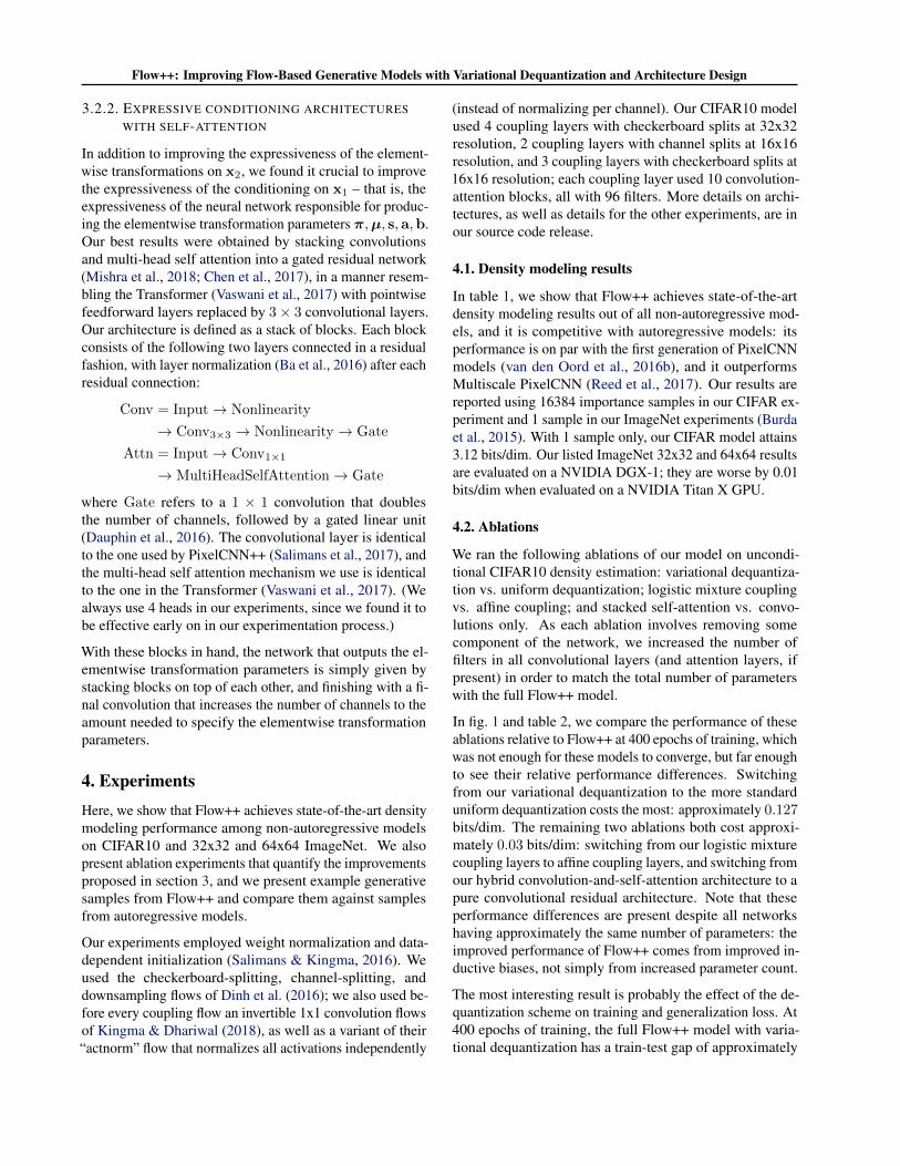
4.1. Density modeling results

In table 1, we show that Flow++ achieves state-of-the-artdensity modeling results out of all non-autoregressive mod-els, and it is competitive with autoregressive models: itsperformance is on par with the first generation of PixelCNNmodels (van den Oord et al., 2016b), and it outperformsMultiscale PixelCNN (Reed et al., 2017). Our results arereported using 16384 importance samples in our CIFAR ex-periment and 1 sample in our ImageNet experiments (Burdaet al., 2015). With 1 sample only, our CIFAR model attains3.12 bits/dim. Our listed ImageNet 32x32 and 64x64 resultsare evaluated on a NVIDIA DGX-1; they are worse by 0.01bits/dim when evaluated on a NVIDIA Titan X GPU.

4.2. Ablations

We ran the following ablations of our model on uncondi-tional CIFAR10 density estimation: variational dequantiza-tion vs. uniform dequantization; logistic mixture couplingvs. affine coupling; and stacked self-attention vs. convo-lutions only. As each ablation involves removing somecomponent of the network, we increased the number offilters in all convolutional layers (and attention layers, ifpresent) in order to match the total number of parameterswith the full Flow++ model.

In fig. 1 and table 2, we compare the performance of theseablations relative to Flow++ at 400 epochs of training, whichwas not enough for these models to converge, but far enoughto see their relative performance differences. Switchingfrom our variational dequantization to the more standarduniform dequantization costs the most: approximately 0.127bits/dim. The remaining two ablations both cost approxi-mately 0.03 bits/dim: switching from our logistic mixturecoupling layers to affine coupling layers, and switching fromour hybrid convolution-and-self-attention architecture to apure convolutional residual architecture. Note that theseperformance differences are present despite all networkshaving approximately the same number of parameters: theimproved performance of Flow++ comes from improved in-ductive biases, not simply from increased parameter count.

The most interesting result is probably the effect of the de-quantization scheme on training and generalization loss. At400 epochs of training, the full Flow++ model with varia-tional dequantization has a train-test gap of approximately


Table 1. Unconditional image modeling results in bits/dimModel family Model CIFAR10 ImageNet 32x32 ImageNet 64x64

Non-autoregressive RealNVP (Dinh et al., 2016) 3.49 4.28 –Glow (Kingma & Dhariwal, 2018) 3.35 4.09 3.81

IAF-VAE (Kingma et al., 2016) 3.11 – –Flow++ (ours) 3.08 3.86 3.69

Autoregressive Multiscale PixelCNN (Reed et al., 2017) – 3.95 3.70PixelCNN (van den Oord et al., 2016b) 3.14 – –PixelRNN (van den Oord et al., 2016b) 3.00 3.86 3.63

Gated PixelCNN (van den Oord et al., 2016c) 3.03 3.83 3.57PixelCNN++ (Salimans et al., 2017) 2.92 – –

Image Transformer (Parmar et al., 2018) 2.90 3.77 –PixelSNAIL (Chen et al., 2017) 2.85 3.80 3.52

Table 2. CIFAR10 ablation results after 400 epochs of training.Models not converged for the purposes of ablation study.

Ablation bits/dim parameters

uniform dequantization 3.292 32.3Maffine coupling 3.200 32.0M

no self-attention 3.193 31.4MFlow++ (not converged for ablation) 3.165 31.4M

0.02 bits/dim, but with uniform dequantization, the train-testgap is approximately 0.06 bits/dim. This confirms our claimin Section 3.1.2 that training with variational dequantiza-tion is a more natural task for the model than training withuniform dequantization.

4.3. Samples

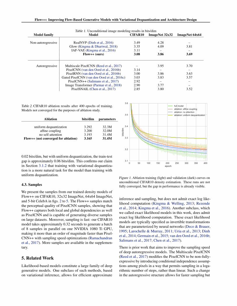
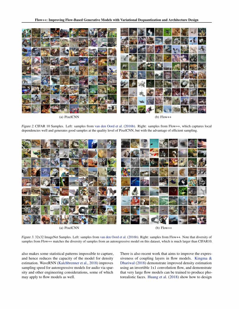
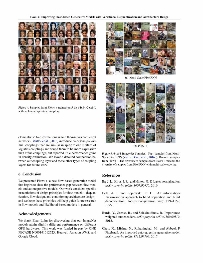
We present the samples from our trained density models ofFlow++ on CIFAR10, 32x32 ImageNet, 64x64 ImageNet,and 5-bit CelebA in figs. 2 to 5. The Flow++ samples matchthe perceptual quality of PixelCNN samples, showing thatFlow++ captures both local and global dependencies as wellas PixelCNN and is capable of generating diverse sampleson large datasets. Moreover, sampling is fast: our CIFAR10model takes approximately 0.32 seconds to generate a batchof 8 samples in parallel on one NVIDIA 1080 Ti GPU,making it more than an order of magnitude faster than Pixel-CNN++ with sampling speed optimizations (Ramachandranet al., 2017). More samples are available in the supplemen-tary.

5. Related WorkLikelihood-based models constitute a large family of deepgenerative models. One subclass of such methods, basedon variational inference, allows for efficient approximate

0 50 100 150 200 250 300 350 400epoch

3.1

3.2

3.3

3.4

3.5

3.6

bits

/dim

full modelablation: affine couplingablation: no attentionablation: uniform dequantization

Figure 1. Ablation training (light) and validation (dark) curves onunconditional CIFAR10 density estimation. These runs are notfully converged, but the gap in performance is already visible.

inference and sampling, but does not admit exact log like-lihood computation (Kingma & Welling, 2013; Rezendeet al., 2014; Kingma et al., 2016). Another subclass, whichwe called exact likelihood models in this work, does admitexact log likelihood computation. These exact likelihoodmodels are typically specified as invertible transformationsthat are parameterized by neural networks (Deco & Brauer,1995; Larochelle & Murray, 2011; Uria et al., 2013; Dinhet al., 2014; Germain et al., 2015; van den Oord et al., 2016b;Salimans et al., 2017; Chen et al., 2017).

There is prior work that aims to improve the sampling speedof deep autoregressive models. The Multiscale PixelCNN(Reed et al., 2017) modifies the PixelCNN to be non-fully-expressive by introducing conditional independence assump-tions among pixels in a way that permits sampling in a loga-rithmic number of steps, rather than linear. Such a changein the autoregressive structure allows for faster sampling but


(a) PixelCNN (b) Flow++

Figure 2. CIFAR 10 Samples. Left: samples from van den Oord et al. (2016b). Right: samples from Flow++, which captures localdependencies well and generates good samples at the quality level of PixelCNN, but with the advantage of efficient sampling.

(a) PixelCNN (b) Flow++

Figure 3. 32x32 ImageNet Samples. Left: samples from van den Oord et al. (2016b). Right: samples from Flow++. Note that diversity ofsamples from Flow++ matches the diversity of samples from an autoregressive model on this dataset, which is much larger than CIFAR10.

also makes some statistical patterns impossible to capture,and hence reduces the capacity of the model for densityestimation. WaveRNN (Kalchbrenner et al., 2018) improvessampling speed for autoregressive models for audio via spar-sity and other engineering considerations, some of whichmay apply to flow models as well.

There is also recent work that aims to improve the expres-siveness of coupling layers in flow models. Kingma &Dhariwal (2018) demonstrate improved density estimationusing an invertible 1x1 convolution flow, and demonstratethat very large flow models can be trained to produce pho-torealistic faces. Huang et al. (2018) show how to design


Figure 4. Samples from Flow++ trained on 5-bit 64x64 CelebA,without low-temperature sampling.

elementwise transformations which themselves are neuralnetworks. Muller et al. (2018) introduce piecewise polyno-mial couplings that are similar in spirit to our mixture oflogistics couplings and found them to be more expressivethan affine couplings, but reported little performance gainsin density estimation. We leave a detailed comparison be-tween our coupling layer and these other types of couplinglayers for future work.

6. ConclusionWe presented Flow++, a new flow-based generative modelthat begins to close the performance gap between flow mod-els and autoregressive models. Our work considers specificinstantiations of design principles for flow models – dequan-tization, flow design, and conditioning architecture design –and we hope these principles will help guide future researchin flow models and likelihood-based models in general.

AcknowledgementsWe thank Evan Lohn for discovering that our ImageNetmodels attain slightly different performance on differentGPU hardware. This work was funded in part by ONRPECASE N000141612723, Huawei, Amazon AWS, andGoogle Cloud.

(a) Multi-Scale PixelRNN

(b) Flow++

Figure 5. 64x64 ImageNet Samples. Top: samples from Multi-Scale PixelRNN (van den Oord et al., 2016b). Bottom: samplesfrom Flow++. The diversity of samples from Flow++ matches thediversity of samples from PixelRNN with multi-scale ordering.

ReferencesBa, J. L., Kiros, J. R., and Hinton, G. E. Layer normalization.

arXiv preprint arXiv:1607.06450, 2016.

Bell, A. J. and Sejnowski, T. J. An information-maximization approach to blind separation and blinddeconvolution. Neural computation, 7(6):1129–1159,1995.

Burda, Y., Grosse, R., and Salakhutdinov, R. Importanceweighted autoencoders. arXiv preprint arXiv:1509.00519,2015.

Chen, X., Mishra, N., Rohaninejad, M., and Abbeel, P.Pixelsnail: An improved autoregressive generative model.arXiv preprint arXiv:1712.09763, 2017.


Dauphin, Y. N., Fan, A., Auli, M., and Grangier, D. Lan-guage modeling with gated convolutional networks. arXivpreprint arXiv:1612.08083, 2016.

Deco, G. and Brauer, W. Higher order statistical decor-relation without information loss. Advances in NeuralInformation Processing Systems, pp. 247–254, 1995.

Dinh, L., Krueger, D., and Bengio, Y. Nice: Non-linearindependent components estimation. arXiv preprintarXiv:1410.8516, 2014.

Dinh, L., Sohl-Dickstein, J., and Bengio, S. Density estima-tion using Real NVP. arXiv preprint arXiv:1605.08803,2016.

Germain, M., Gregor, K., Murray, I., and Larochelle, H.Made: Masked autoencoder for distribution estimation.arXiv preprint arXiv:1502.03509, 2015.

Goodfellow, I., Pouget-Abadie, J., Mirza, M., Xu, B.,Warde-Farley, D., Ozair, S., Courville, A., and Bengio,Y. Generative adversarial nets. In Advances in neuralinformation processing systems, pp. 2672–2680, 2014.

Huang, C.-W., Krueger, D., Lacoste, A., and Courville, A.Neural autoregressive flows. In International Conferenceon Machine Learning, pp. 2083–2092, 2018.

Hyvarinen, A. and Pajunen, P. Nonlinear independent com-ponent analysis: Existence and uniqueness results. NeuralNetworks, 12(3):429–439, 1999.

Hyvarinen, A., Karhunen, J., and Oja, E. Independentcomponent analysis, volume 46. John Wiley & Sons,2004.

Kalchbrenner, N., Espheholt, L., Simonyan, K., Oord,A. v. d., Graves, A., and Kavukcuoglu, K. euralmachine translation in linear time. arXiv preprintarXiv:1610.00527, 2016a.

Kalchbrenner, N., Oord, A. v. d., Simonyan, K., Danihelka,I., Vinyals, O., Graves, A., and Kavukcuoglu, K. Videopixel networks. arXiv preprint arXiv:1610.00527, 2016b.

Kalchbrenner, N., Elsen, E., Simonyan, K., Noury, S.,Casagrande, N., Lockhart, E., Stimberg, F., Oord, A.v. d., Dieleman, S., and Kavukcuoglu, K. Efficient neuralaudio synthesis. arXiv preprint arXiv:1802.08435, 2018.

Karras, T., Aila, T., Laine, S., and Lehtinen, J. Progres-sive growing of gans for improved quality, stability, andvariation. arXiv preprint arXiv:1710.10196, 2017.

Kingma, D. P. and Dhariwal, P. Glow: Generativeflow with invertible 1x1 convolutions. arXiv preprintarXiv:1807.03039, 2018.

Kingma, D. P. and Welling, M. Auto-encoding variationalBayes. Proceedings of the 2nd International Conferenceon Learning Representations, 2013.

Kingma, D. P., Salimans, T., and Welling, M. Improv-ing variational inference with inverse autoregressive flow.arXiv preprint arXiv:1606.04934, 2016.

Larochelle, H. and Murray, I. The Neural AutoregressiveDistribution Estimator. AISTATS, 2011.

Louizos, C. and Welling, M. Multiplicative normalizingflows for variational bayesian neural networks. arXivpreprint arXiv:1703.01961, 2017.

Mishra, N., Rohaninejad, M., Chen, X., and Abbeel, P. Asimple neural attentive meta-learner. In InternationalConference on Learning Representations (ICLR), 2018.

Muller, T., McWilliams, B., Rousselle, F., Gross, M., andNovak, J. Neural importance sampling. arXiv preprintarXiv:1808.03856, 2018.

Parmar, N., Vaswani, A., Uszkoreit, J., Kaiser, Ł., Shazeer,N., and Ku, A. Image transformer. arXiv preprintarXiv:1802.05751, 2018.

Ramachandran, P., Paine, T. L., Khorrami, P., Babaeizadeh,M., Chang, S., Zhang, Y., Hasegawa-Johnson, M. A.,Campbell, R. H., and Huang, T. S. Fast generationfor convolutional autoregressive models. arXiv preprintarXiv:1704.06001, 2017.

Reed, S. E., van den Oord, A., Kalchbrenner, N., Gomez,S., Wang, Z., Belov, D., and de Freitas, N. Parallel multi-scale autoregressive density estimation. In Proceedings ofThe 34th International Conference on Machine Learning,2017.

Rezende, D. and Mohamed, S. Variational inference withnormalizing flows. In Proceedings of The 32nd Interna-tional Conference on Machine Learning, pp. 1530–1538,2015.

Rezende, D. J., Mohamed, S., and Wierstra, D. Stochas-tic backpropagation and approximate inference in deepgenerative models. In Proceedings of the 31st Interna-tional Conference on Machine Learning (ICML-14), pp.1278–1286, 2014.

Salimans, T. and Kingma, D. P. Weight normalization: Asimple reparameterization to accelerate training of deepneural networks. arXiv preprint arXiv:1602.07868, 2016.

Salimans, T., Karpathy, A., Chen, X., and Kingma, D. P.Pixelcnn++: Improving the pixelcnn with discretized lo-gistic mixture likelihood and other modifications. arXivpreprint arXiv:1701.05517, 2017.


Theis, L., Oord, A. v. d., and Bethge, M. A note onthe evaluation of generative models. arXiv preprintarXiv:1511.01844, 2015.

Uria, B., Murray, I., and Larochelle, H. Rnade: The real-valued neural autoregressive density-estimator. In Ad-vances in Neural Information Processing Systems, pp.2175–2183, 2013.

van den Oord, A., Dieleman, S., Zen, H., Simonyan, K.,Vinyals, O., Graves, A., Kalchbrenner, N., Senior, A., andKavukcuoglu, K. Wavenet: A generative model for rawaudio. arXiv preprint arXiv:1609.03499, 2016a.

van den Oord, A., Kalchbrenner, N., and Kavukcuoglu, K.Pixel recurrent neural networks. International Conferenceon Machine Learning (ICML), 2016b.

van den Oord, A., Kalchbrenner, N., Vinyals, O., Espeholt,L., Graves, A., and Kavukcuoglu, K. Conditional im-age generation with pixelcnn decoders. arXiv preprintarXiv:1606.05328, 2016c.

Vaswani, A., Shazeer, N., Parmar, N., Uszkoreit, J., Jones,L., Gomez, A. N., Kaiser, L., and Polosukhin, I. Attentionis all you need. arXiv preprint arXiv:1706.03762, 2017.

Flow++: Improving Flow-Based Generative Models with VariationalDequantization and Architecture Design – Supplementary Material

In subsequent pages, we present more Flow++ samples for CIFAR 10, 32 x 32 Imagenet, 64 x 64 Imagenet, 64 x 64 Imagenetwith 5-bits per color channel, 64 x 64 CelebA HQ with 3-bits per color channel and 64 x 64 CelebA HQ with 5-bits percolor channel.

Our implementation can be found at https://github.com/aravindsrinivas/flowpp.



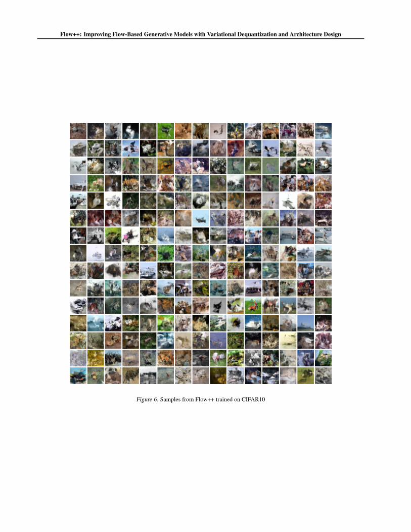
Figure 6. Samples from Flow++ trained on CIFAR10


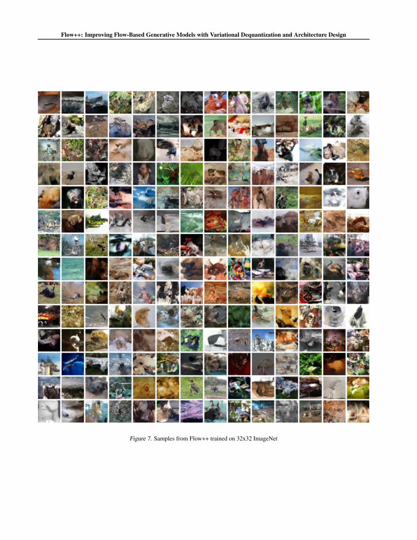
Figure 7. Samples from Flow++ trained on 32x32 ImageNet


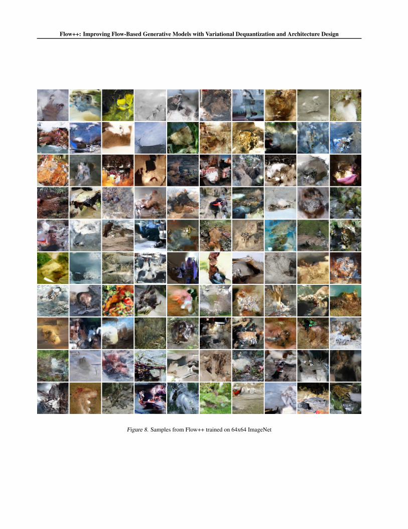
Figure 8. Samples from Flow++ trained on 64x64 ImageNet


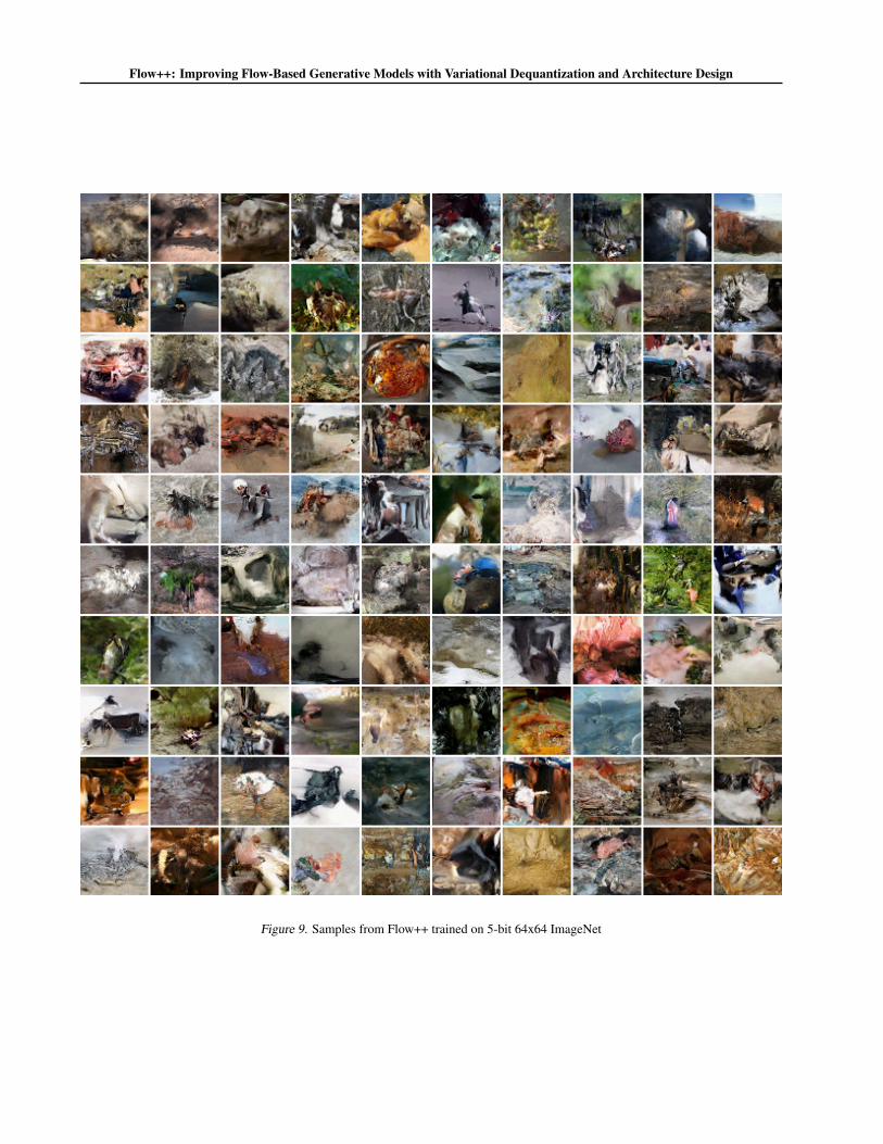
Figure 9. Samples from Flow++ trained on 5-bit 64x64 ImageNet


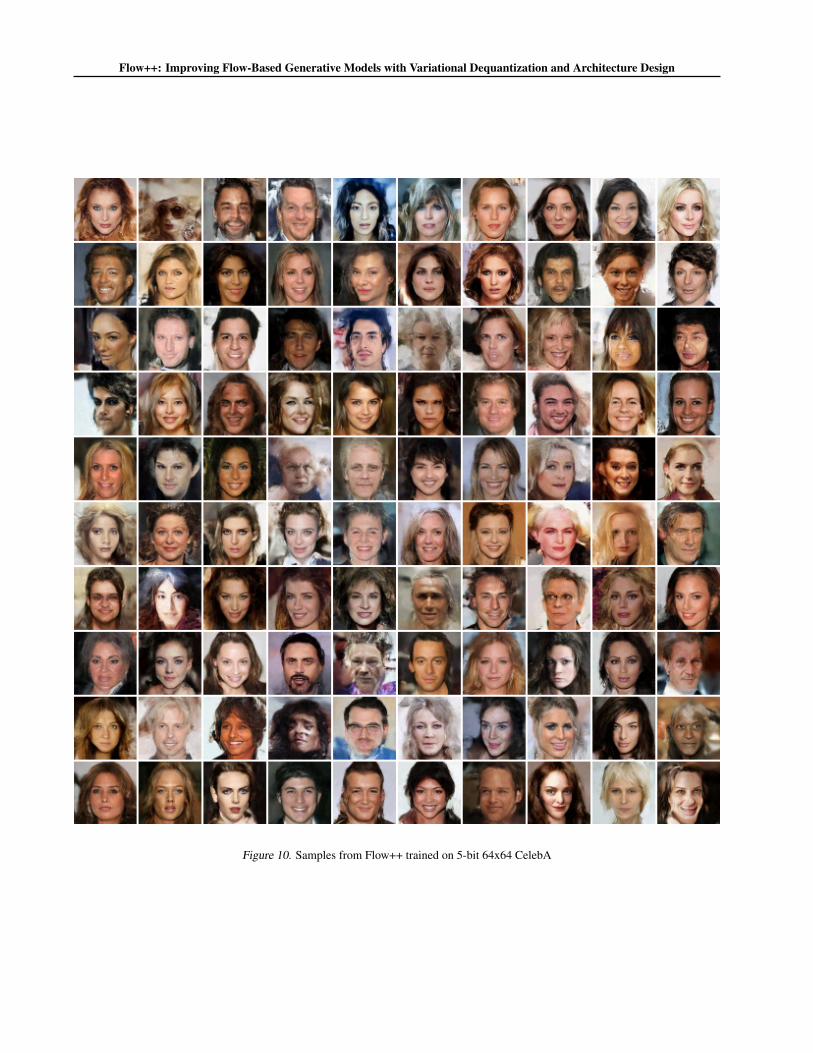
Figure 10. Samples from Flow++ trained on 5-bit 64x64 CelebA


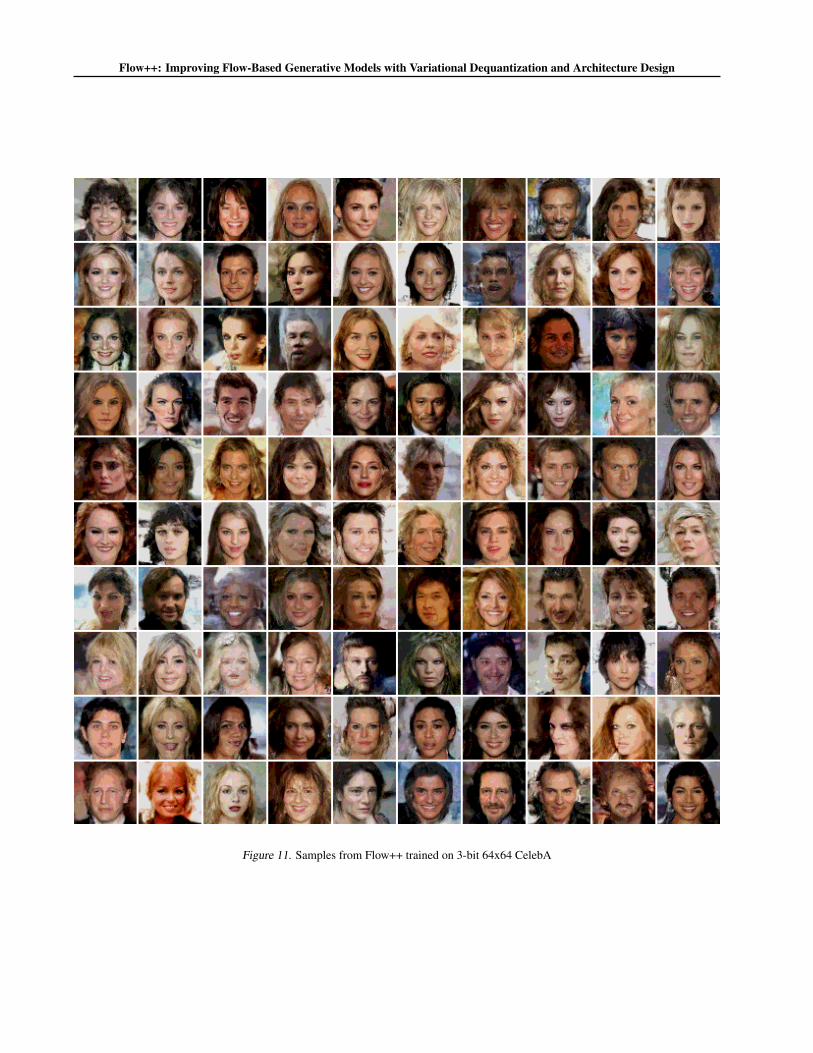
Figure 11. Samples from Flow++ trained on 3-bit 64x64 CelebA

Documents

Flow++: Improving Flow-Based Generative Models with ... · 1. Introduction Deep generative models – latent variable models in the form of variational autoencoders (Kingma & Welling,2013),