Flow in compound channel with abrupt floodplain contraction

HAL Id: hal-00274829https://hal.archives-ouvertes.fr/hal-00274829

Submitted on 15 May 2020

HAL is a multi-disciplinary open accessarchive for the deposit and dissemination of sci-entific research documents, whether they are pub-lished or not. The documents may come fromteaching and research institutions in France orabroad, or from public or private research centers.

L’archive ouverte pluridisciplinaire HAL, estdestinée au dépôt et à la diffusion de documentsscientifiques de niveau recherche, publiés ou non,émanant des établissements d’enseignement et derecherche français ou étrangers, des laboratoirespublics ou privés.

Flow in compound channel with abrupt floodplaincontraction

S. Proust, Nicolas Riviere, D. Bousmar, André Paquier, Y. Zech, R. Morel

To cite this version:S. Proust, Nicolas Riviere, D. Bousmar, André Paquier, Y. Zech, et al.. Flow in compound channelwith abrupt floodplain contraction. Journal of Hydraulic Engineering, American Society of CivilEngineers, 2006, 132 (9), pp.958-970. �10.1061/(ASCE)0733-9429(2006)132:9(958)�. �hal-00274829�

https://hal.archives-ouvertes.fr/hal-00274829

https://hal.archives-ouvertes.fr

FLOW IN COMPOUND CHANNEL WITH ABRUPT FLOOD PLAIN

CONTRACTION

S. Proust1, N. Rivière

2, D. Bousmar

3, A. Paquier

4, Y. Zech

5, R. Morel

6

ABSTRACT :

Flooding rivers usually present transition reaches where the floodplain width can significantly

vary. The present study focuses on an abrupt floodplain contraction (mean angle 22°) in order

to determine whether one-dimensional (1D) models, developed for straight and slightly

converging geometry, are equally valid for such a geometry. Experiments on a contraction

model were carried out in an asymmetric compound channel flume. Severe mass and

momentum transfers from the floodplain towards the main channel were observed, giving rise

to a noteworthy transverse slope of the water surface and different head loss gradients in the

two subsections. Three 1D models and one 2D simulation were compared to experimental

measurements. Each 1D model incorporates a specific approach for the modeling of the

momentum exchange at the interface boundary between the main channel and the floodplain.

The increase of the lateral mass transfer generates moderate errors on the water level values

but significant errors on the discharge distribution. Erroneous results arise because of

incorrect estimations of both momentum exchange due to lateral mass transfers and boundary

conditions which are imposed by the tested 1D models.

CE Database subject headings : Open channels; Nonuniform flow; Flood plains;

Experimental data; Numerical models; Mass transfer; Contraction.

__________________________________________________________________________

1 Researcher, Hydrology-Hydraulics unit, Cemagref Lyon, Quai Chauveau, 3bis, CP 220 - 69336 Lyon Cedex

09, France. E-mail: [email protected].

2 Assistant Professor, LMFA, INSA de Lyon, Av. Einstein, 20, 69621 Villeurbanne Cedex, France. E-mail:

[email protected].

Author-produced version of the article published in Journal of Hydraulic Engineering, 2006, vol.132, n°9, p. 958-970 The original publication is available at : http://cedb.asce.org, doi:10.1061/(ASCE)0733-9429(2006)132:9(958)

3 Formerly Postdoctoral Researcher, Fond National de la Recherche Scientifique; Now Engineer, Laboratory of

Hydraulic Research (D.213), Ministère wallon de l'Equipement et des Transports, Rue de l'Abattoir, 164, 6200

Châtelet, Belgium. E-mail: [email protected]..

4 Researcher, Hydrology-Hydraulics unit, Cemagref Lyon, Quai Chauveau, 3bis, CP 220 - 69336 Lyon Cedex

09, France. E-mail: [email protected].

6 Professor, Dept. of Civil and Environmental Engineering, Hydraulics Unit, Université catholique de Louvain,

Place du Levant, 1, 1348 Louvain-la-Neuve, Belgium. E-mail: [email protected].

6 Professor, LMFA, INSA de Lyon, Av. Einstein, 20, 69621 Villeurbanne Cedex, France. E-mail:

[email protected].

__________________________________________________________________________________________

INTRODUCTION

In the computation of water profile and discharge distribution of overbank flow in

rivers, the transition reaches require special attention. Indeed, they are the place of significant

mass exchanges between subsections that give birth to noteworthy 3D physical phenomena.

2D or 3D simulations can logically be appropriate for such reaches. However, this paper

emphasizes on one-dimensional models since they are still widely used for backwater

computations and flood plain discharge calculation when modeling a complete river system.

Thus, from an engineering point of view, it seems necessary to test the relevance of classical

1D models for transition reaches, to identify the most restrictive assumptions of such models,

and to evaluate the opportunity of a specific treatment. It should be noted that such models

have shown their effectiveness for non-prismatic compound channel when mass transfers are

moderate.

Most previous experiments in compound channels have been performed under uniform

flow conditions in straight floodplains, with prismatic or meandering main channels (see e.g.

Shiono and Knight 1991, Wormleaton and Merrett 1990, Sellin et al. 1993, Abril and Knight

2004, Martin-Vide et al. 2004). Particularly, studies based on the data collected in the large

scale Flood Channel Facility, H.R. Wallingford, U.K., are mainly focused on the conveyance

evaluation, the flow pattern description in the composite section, and the bed shear stress


distribution (Knight et al. 1994). Flow-width transitions were not often explored except for

bridges across floodplains, and mostly in the case of single channel (Hunt et al. 1999). Only

few studies were devoted to non-prismatic floodplain flows: Bousmar et al. (2004) with two

symmetrical narrowing floodplains (angle between 3.8° and 11.3°); Elliot and Sellin (1990)

with the case of skewed flows in a compound channel (skew angle of 2°, 5° and 9°); Jasem

(1990) for similar skewed flows but at a smaller scale; Sturm and Janjua (1994) with a groyn

in the floodplain focusing on scouring. The present study of the flow in an abrupt floodplain

contraction (mean angle 22° ) extends those previous works to more rapidly varied conditions.

Experimental data were collected in an asymmetric compound channel flume at the

laboratory of the Compagnie Nationale du Rhône, Lyon, France (Fig.1). The flow structure is

characterized by: (1) a domination of the mass exchanges compared to turbulent transfers; and

(2) the presence of secondary current cells in the main channel. The overbank flow rolls over

the inbank one, inducing a horizontal shear and associated secondary-current cells as observed

in skewed or meandering compound channels (Shiono & Muto 1998). A notable transverse

water surface slope appears at the approach to the end of the converging reach, in relation

with the mass transfer between both beds. The coexistence of supercritical flow in the

floodplain and subcritical flow in the main channel is also observed in this area. Eventually,

the evolution of the subsection-averaged head, as defined by Yen (2002), is different from the

main channel to the floodplain.

Considering such a flow, the attention is focused on the ability of 1D-approaches with

different levels of complexity to model physical phenomena. Notably, relations validated for

symmetrically narrowing floodplains (Bousmar 2002, Bousmar et al. 2004) are evaluated in

this configuration.

First, experimental values of the main hydraulic parameters are presented and

analyzed. Then, different 1D modellings of interfacial exchanges between the main channel


and the floodplain are exposed and compared to experimental results. Each approach has a

specific treatment of the interfacial transfers: (1) the classical Divided Channel Method

(DCM) used by HEC-RAS ignores the momentum transfer through subsection boundaries; (2)

the Exchange Discharge Model (EDM), implemented in the program Axeriv, accounts for

both mass and turbulent exchanges (Bousmar and Zech 1999); (3) and the Debord Formula,

used in the program Talweg-Fluvia, proposes an empirical correction of the DCM that merely

models the turbulent transfer (Nicollet and Uan 1979). Then, 2D calculations are performed

with the program Mac2D (Bousmar 2002), in order to shed light on the phenomena that are

not taken into account by those 1D-approaches. Notably, 1D and 2D head loss gradients are

compared.

This analysis helps to understand the calculated water profiles and discharge

distribution evolution, obtained by Hec-RAS, Talweg-Fluvia, and Axeriv.

EXPERIMENTAL SET-UP AND MEASURING TECHNIQUES

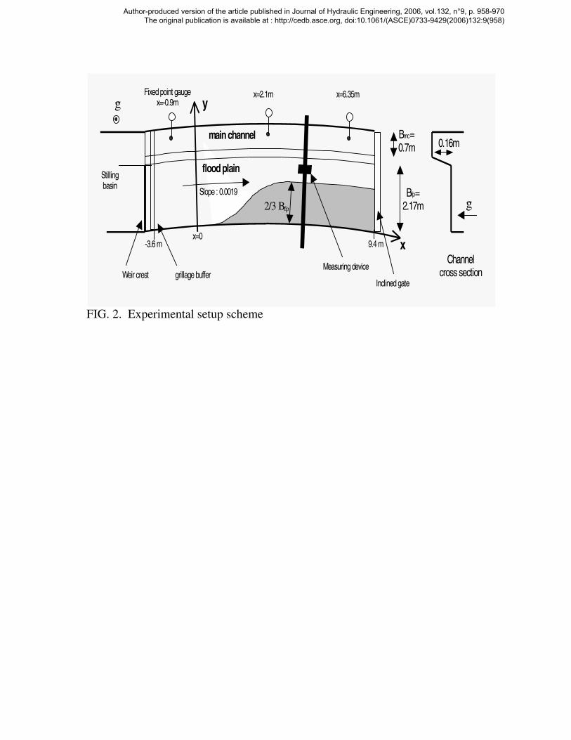
New experiments were performed in a compound channel flume of length L = 13 m

and total width B = 2.97 m, with a bed slope S0 = 1.9 x 10-3

(Fig. 1 and 2). As this set-up was

primarily used to reproduce an existent river dynamics, it exhibited a slight curvature, with an

approximate radius 25 m. The reference xyz was defined with x-axis always parallel to the

right side of the flood plain. The bed was cement covered with different ridges orientated so

as to obtain different surface roughness in the main channel and in the floodplain. The

bankfull depth was 0.16 m deep below the flood plain level, while its bottom width was Bmc =

0.7 m. The bank presented a constant slope of 32° between the main channel and the

floodplain. The floodplain width was Bfp = 2.17 m. An obstacle was set on the floodplain

(Fig. 1 and 2), presenting a strong convergence of length 350 cm and of projected width 143


cm perpendicularly to the main flow direction (mean angle of 22°). The flow was studied

between x = 0 and 4.5 m.

A stilling basin preceded the entrance of the compound channel, and the flow stilling

was achieved by honeycombs of bricks and wire netting buffers. Due to the small length to

width ratio L/B, particular attention was devoted to supply the channel with a discharge

distribution between subsections close to the one observed in uniform flow conditions (Proust

et al. 2002, Bousmar et al. 2005). For this purpose, the inlets of the two channels were

separated in the stilling basin. A sharp-crested weir was placed at the inlet of the floodplain in

order to limit its discharge Qfp compared to the main channel discharge Qmc for a given depth

in the basin. At the downstream end of the channel, an inclined gate was used to set a constant

water depth in uniform-flow conditions. Two discharges were investigated during the

experiments to highlight the influence of the relative water depth (See- Tab. 1).

Water levels were measured by a moveable point gauge. The accuracy was ± 0.15 mm,

but could worsen to ± 0.3 mm in areas where the surface was strongly perturbed (i.e. in the

vicinity of the obstacle and just after the stilling basin). Velocities were measured using a

miniature propeller of 1 cm diameter for the lower discharge; and an acoustic Doppler

Velocimeter (Nortek NDV 2D-3D side-looking probe) for the larger one. In addition to the

propeller measurements, the main deviation of the velocity to the x-direction was measured

using a homemade miniature vane, with an accuracy of about ± 2°. Depth-averaged velocities

were obtained from 4 measurements on each vertical in the main channel, and from 3

measurements in the flood plain. Four vertical profiles were recorded in the main channel, and

between 4 and 10 in the floodplain (Fig.4) in order to determine the depth-averaged velocity

distribution. The subsection and total discharges were estimated by integration of the

velocities on cross-section areas. The so-estimated total discharges were found to be within –


1/+6 % of the discharge measured by an electromagnetic flowmeter installed on the supply

pipe.

The roughness coefficient values were calibrated from uniform flow conditions. Seven

uniform flows were obtained in the main channel, and two in the floodplain, by separating

both subsections by a wall at the interface. Using the Manning formula leads to roughness

values of 0.0119 and 0.0132 s/m1/3

in the main channel and in the floodplain, respectively.

The associated sand grain roughness ks = 0.0006 and ks = 0.0014 mm, correspond to values

between concrete class 3 and class 4 (French 1985, Tab. 4.1 p 116). The same roughness

values were used for the flow in the abrupt floodplain. The large values of Reynolds numbers

(from 16000 to 170000) at any studied station x of the whole reach assure a fully rough

turbulent flow in both subsections, and a Manning roughness coefficient independent of the

hydraulic radius Rh (French 1985).

EXPERIMENTAL RESULTS

In order to test the relevance of 1D models for non-prismatic compound channels, the

flow configuration was designed to enhance the longitudinal variations of the hydraulic

parameters. This should enable the assessment of methods developed for slightly non-

prismatic compound channels. In order to discuss the standard 1D assumptions, some

variables such as subsection-averaged values (water depths, velocities, discharges, one-

dimensional head) were defined in spite of the flow heterogeneity, especially in the

floodplain. Their relevance is discussed below.

Water levels

The transverse water level distribution is given for the higher discharge, Q = 260 l/s,

on Fig 3. Due to the contraction abruptness and the centrifugal effects, transverse gradients of

these levels are observed for x = 4.5 m, with differences in the range 20-25 % of the


floodplain mean flow depth for Q = 150 and 260 l/s. It is important to notice that the channel

curvature influence, measured in uniform flows conditions, is of a lower magnitude order.

Consequently, the longitudinal water surface slopes are different from subsection to

subsection at the approach to the end of the converging reach. The drop of the free surface

level along the x-axis can also be related to the velocities increase. Variations of the relative

flow depth hr= hfp/hmc are presented in Tab.1

Velocity field

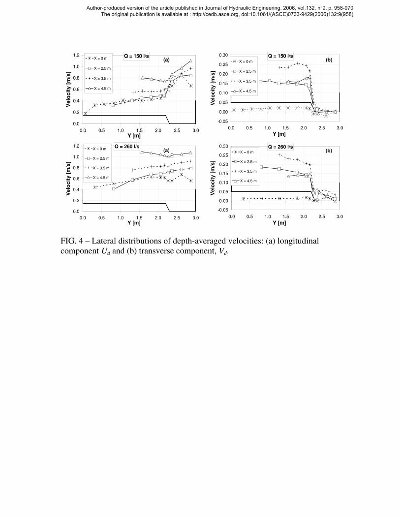
The transverse distribution of depth-averaged velocity components are presented on

Fig. 4: Ud is the longitudinal component, and Vd, the transverse one. As part of the flow is

forced to leave the floodplain, a transverse current develops, and downstream, the velocities

become constant across the section width due to the contraction for the higher discharge. In

the upper part of the reach, the velocity gradient between the main channel and the floodplain

is less noticeable for Q = 260 l/s than for the lower discharge, due to the higher relative flow

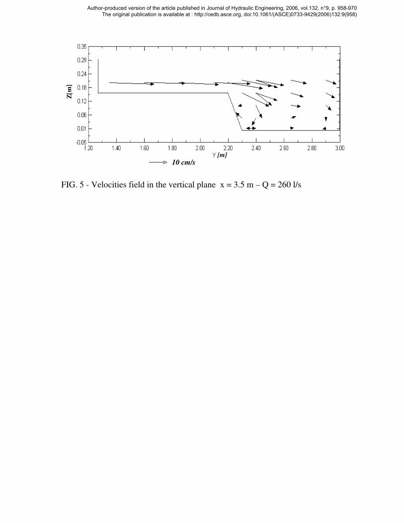
depth hr. Fig. 5 presents the lateral v- and vertical w-components of velocities, measured for

the higher discharge, at the station x = 3.5 m. The overbank flow rolls over the inbank one

towards the main channel bank opposite to the floodplain. This generates an helical motion

that increases along the x-axis. The flow pattern-direction in the main channel close to the

bottom (at 0.2hmc) is thus different from the one close to the surface (Fig.6). This flow

structure presents similarities with the one observed in the main channel of slightly narrowing

(Bousmar et al. 2004), skewed (Elliot & Sellin 1990) or meandering (Shiono & Muto 1998)

compound channels.

Discharge distribution

The evolution of the discharge distribution along the studied reach is presented on Fig.

7, through the discharge floodplain as percentage of the total discharge Qfp/Q (x 100).


Between x = 0 and x = 4.5 m, 75% and 54% of the floodplain discharge is transferred to the

main channel for the lower and higher discharges respectively.

Head evolution

A subsection-averaged head, Hsub, can be defined in the x-direction, accounting for

transverse variations of u and v-components of local velocity (Lancastre 1999) and water

levels Z(y) from an eulerian point of view.

( )

∫∫

∫∫

∫∫

∫∫+

+=

sub

sub

sub

sub

A

A

A

A

subudA

dAug

vu

udA

udAyZH

2

²²)(

(1)

where Z(y) = Zb + h(y), Zb = bed level above reference datum, and dA=dz.dy. The total head,

H, is defined in a same way on the whole cross-section area. The experimental head profiles

computed in the whole cross-section, in both subsections are shown on Fig. 8. The influence

of v-components is experienced on the total head H.

Noticeable differences on the head evolution are observed on the three profiles, for

both discharges. This is due to a different evolution of the kinetic energy term in (1) along the

channel in both subsections, in addition to a different evolution of water levels near the end of

the converging reach. This could make inconsistent the 1D models that assume the same head

evolution in all subsections when transfers between subsections are moderate. These models

suggest that a river adjusts its energy budget along the flow (Bousmar and Zech 1999). As

mass transfers become severe in the present abrupt contraction, this equality is not true any

longer. This statement confirms previous assumptions by Yen (2002), that were not yet

verified using experimental data. Accordingly, the flow can not adjust its energy budget

within the whole cross-section when mass and energy transfers increase, because of inertial

phenomena. A delay is also identified between the mass transfer and the water surface lateral

inclination for both discharges: at station x = 3.5 m where the measured mass exchanges are


the most significant (Fig. 4, Vd-components) , the transverse water surface is horizontal,

contrarily to the situation for x = 4.5 m (Fig. 3).

Secondly, a slight influence of v-components on the total head H is observed for the

higher discharge.

Eventually, as most 1D models consider a unique water level across the whole section

of the compound channel, the influence of such a simplification on the subsection head

evolution had to be assessed. The interaction between lateral and longitudinal gradients of the

water levels is exposed in Rivière et al. (2002) and found significant. It generates an

overestimation of the head slope in the main channel and in the whole section. It would thus

introduce in that context a noteworthy redistribution of energy between subsections close to

the end of the converging reach. This is a possible cause of errors in the prediction of

hydraulic parameters by the 1D models, if computation starts from the downstream part of the

reach.

Froude numbers

Noticeable differences can be observed between the one-dimensional Froude numbers

estimated in each subsection of the compound channel. For both discharge rates, a

juxtaposition of supercritical flow conditions in the floodplain and subcritical flow conditions

in the main channel appears in the downstream part of the reach, between x = 3.5 and 4.5 m.

At the narrowest section (x = 4.5 m), for Q = 260 l/s (resp. 150 l/s), one gets : Frmc = 0.67

(resp. 0.7) in the main channel, and Frfp =1.22 (resp. 1.3) in the floodplain.


MODELLING OF INTERFACIAL TRANSFERS

Presentation of the different 1D models

The relevance of 1D-approaches for compound channel is related to the accuracy of

interfacial transfer modeling. The significance of these interfacial shear stresses and lateral

discharges between subsections was investigated for backwater profiles computation in

straight compound channel (Yen 1984, Yen et al. 1985), and more recently for slightly non-

prismatic geometries (Bousmar and Zech 1999, Bousmar et al. 2004). Both approaches

distinguish the mass exchange and turbulence exchange contributions in the interfacial

momentum transfer.

The first 1D modelling considered in the following analysis is the classical Divided

Channel Method (DCM), which is the reference case since it ignores both turbulent and mass

transfers between subsections.

The Bousmar and Zech (1999) model, called Exchange Discharge Method (EDM) is

the second modelling investigated. EDM is based on a theoretical modelling of the interfacial

momentum transfer, tested for flows in slightly skewed compound channels and for a

compound channel with narrowing floodplains. The interfacial shear on the subsection

boundary is evaluated by using a mixing length model in the horizontal plane, and by

expressing a turbulent exchange lateral discharge, noted qt, and modeled by:

qt = 0.16.hfp (Umc-Ufp). (2)

where hfp is the mean flow depth on the floodplain, and the value 0.16 is a coefficient that was

calibrated from nine series of uniform flows in the FCF of HR Wallingford (Bousmar and

Zech 1999).


The mass exchange is represented by a lateral mass discharge qm = |dQfp/dx|. EDM takes the

momentum transfer due to this mass exchange into account. However, this model can be used

considering the turbulent momentum transfer only: it will be designated in that case as EDM*.

The last modelling under consideration is the Debord formula (Nicollet and Uan

1979). It is an empirical method that was developed on the basis of large experimental data

sets in a 60 m x 3 m straight compound-channel flume. The Debord formula gives an estimate

of the conveyance on the whole cross-section, K*, by modifying the one of the DCM as

follows:

( ) 3/2223/2* )1(11

.fphfpmcfp

fp

mcmch

mc

RAAAn

ARn

K ϕϕ −++= (3)

whereϕ is a parameter that accounts for turbulent exchanges, modeled by:

( )

[ ] ( ) [ ]{ }oo

fpmco

r

nn

ϕπϕϕ

ϕϕ

++−=

==

13.0/cos12

1

9.06/1

if 3.0

3.0

≤=

≥=

mchfph

mchfph

RRr

RRr (4)

In that way, it is close to more recent empirical formulae such as Ackers’ (1991, 1992)

or to previous expressions proceeding from the computation of an apparent shear stress acting

at the interfacial boundary (Knight & Demetriou 1983, Wormleaton & Merett 1990). The

Debord method has been extensively used for more than 20 years by French modelers. It

accounts for turbulent transfers but not for mass exchanges in the momentum transfers.

Influence of possible turbulent exchanges on discharge distribution modelling

In order to evaluate the contribution of possible turbulent exchanges related to the

velocity gradient between subsections, the subsection-averaged values of discharge and

velocity were calculated at each measurement station of the reach, for equivalent uniform

flows of same cross-section area, using the actual experimental water level, averaged on the

whole width. Three different calculations were conducted: with the DCM (reference


calculation), with the EDM* and with Debord. Fig. 7 gives the resulting floodplain

discharges, and Tab. 2 presents the relative errors between computed and experimental values.

The floodplain discharge computed by the DCM deviates from the experiments towards

downstream, with a maximum discrepancy of –57 % (resp. -37%) at the last station for Q =

150 l/s (resp. 260 l/s). This indicates the significance of interfacial transfers (mass and/or

turbulence) in the evaluation of the discharge distribution. Considering possible turbulent

exchanges reduces the discrepancies, but the floodplain discharge is still noticeably

underestimated downstream (-34 % for Q = 150 l/s and the Debord formula).

Fig. 9 presents the experimental mean velocities in the floodplain, the values

calculated by the Debord formula, the DCM and EDM*. Experimental values computed with

the actual subsection discharges but with an averaged value of the water level across the

whole width (Zmean) instead of the actual subsection level (Zsub) are also given, in order to

evaluate the influence of the transverse water slope in the downstream part. Debord and

EDM* model experimental values between the first two stations (0m < x < 2.5m) accurately.

Notable differences between DCM values and experimental ones highlight the role of the

interfacial turbulent exchange modelling. Not considering the mass exchange in the

momentum transfer is not prejudicial in this upstream part of the reach. Between x = 3.5 and

4.5 m the DCM values are noticeably erroneous, with a maximum error of 62 % for Q = 150

l/s. Values of Debord and EDM* are closer to experimental results, but an underestimation of

the mean velocity of 39 % at x = 4,5 m clearly demonstrates that accounting only for possible

turbulent transfer is not sufficient. Assuming a unique water level in a cross-section cannot

explain this discrepancy, since it gives an error of 9% on the floodplain mean velocity only.

The increasing difference between DCM, and Debord and EDM* towards

downstream, is in agreement with the literature (Ackers 1991): as the relative water depth hr

is decreasing, the role of turbulence transfer for the equivalent uniform flow is increasing.


However, near the reach end, the gradient of experimental velocity between the main channel

and the floodplain is quite low for Q = 150 l/s and even nil for Q = 260 l/s (Fig. 4, Ud-

components). Measurements of the Reynolds stresses ρu’v’ obtained with the NDV probe for

the higher discharge confirm the low level of the associated turbulence. The increase of the

floodplain velocity is in fact due to mass exchange, as 2D modeling will also prove hereafter.

Accordingly, Debord and EDM* artificially add dissipation between both subsections, by

means of turbulent exchanges due to a velocity gradient not physically observed in the

downstream part of the reach. Adding such an artificial momentum transfer reduces prediction

errors on both discharge distribution and subsection velocities.

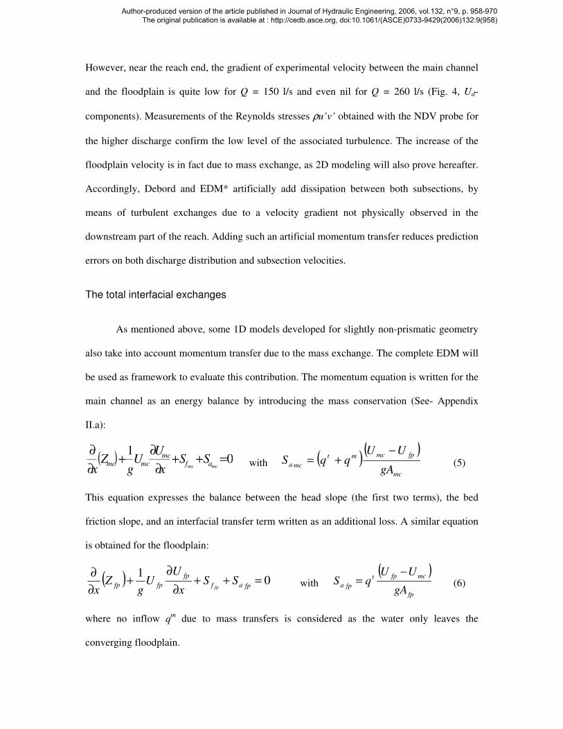
The total interfacial exchanges

As mentioned above, some 1D models developed for slightly non-prismatic geometry

also take into account momentum transfer due to the mass exchange. The complete EDM will

be used as framework to evaluate this contribution. The momentum equation is written for the

main channel as an energy balance by introducing the mass conservation (See- Appendix

II.a):

( ) 01

=++∂

∂+

∂

∂mcmc af

mcmcmc SS

x

UU

gZ

x with ( )

( )mc

fpmcmt

mcagA

UUqqS

−+= (5)

This equation expresses the balance between the head slope (the first two terms), the bed

friction slope, and an interfacial transfer term written as an additional loss. A similar equation

is obtained for the floodplain:

( ) 01

=++∂

∂+

∂

∂fpaf

fp

fpfp SSx

UU

gZ

x fp with

( )fp

mcfpt

fpagA

UUqS

−= (6)

where no inflow qm due to mass transfers is considered as the water only leaves the

converging floodplain.


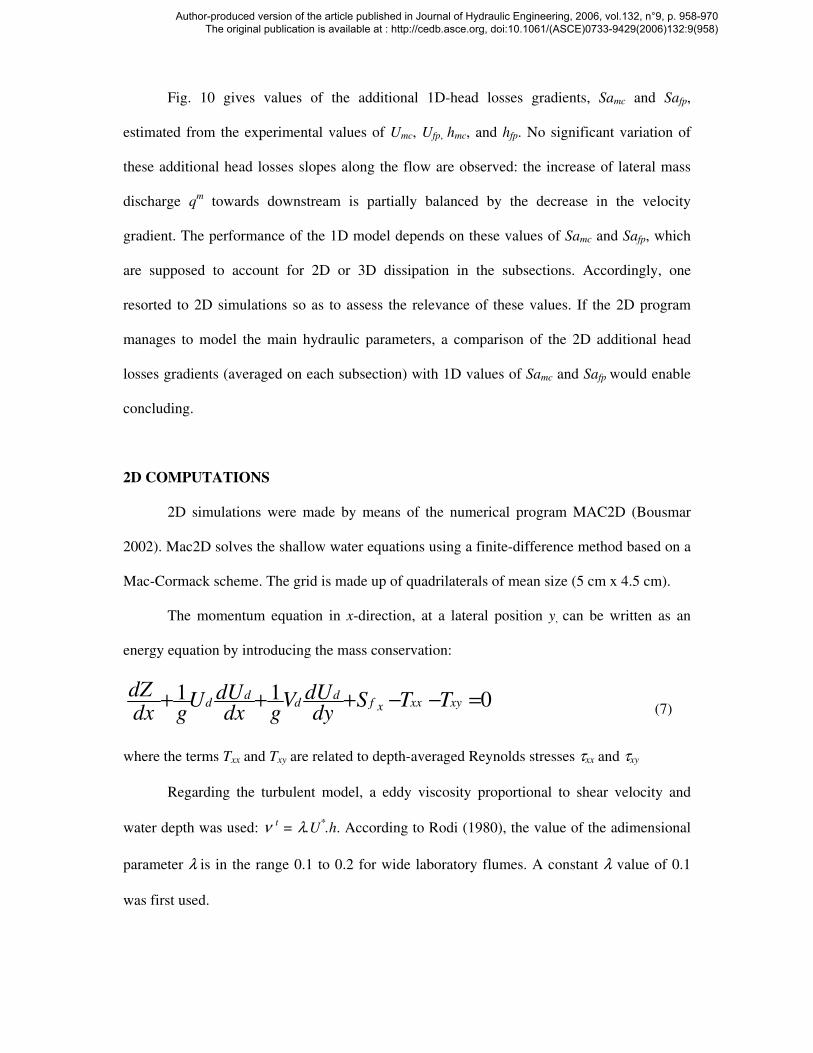
Fig. 10 gives values of the additional 1D-head losses gradients, Samc and Safp,

estimated from the experimental values of Umc, Ufp, hmc, and hfp. No significant variation of

these additional head losses slopes along the flow are observed: the increase of lateral mass

discharge qm towards downstream is partially balanced by the decrease in the velocity

gradient. The performance of the 1D model depends on these values of Samc and Safp, which

are supposed to account for 2D or 3D dissipation in the subsections. Accordingly, one

resorted to 2D simulations so as to assess the relevance of these values. If the 2D program

manages to model the main hydraulic parameters, a comparison of the 2D additional head

losses gradients (averaged on each subsection) with 1D values of Samc and Safp would enable

concluding.

2D COMPUTATIONS

2D simulations were made by means of the numerical program MAC2D (Bousmar

2002). Mac2D solves the shallow water equations using a finite-difference method based on a

Mac-Cormack scheme. The grid is made up of quadrilaterals of mean size (5 cm x 4.5 cm).

The momentum equation in x-direction, at a lateral position y, can be written as an

energy equation by introducing the mass conservation:

011 =−−+++ xyxxxfd

dd

d TTSdy

dUVgdx

dUUgdx

dZ (7)

where the terms Txx and Txy are related to depth-averaged Reynolds stresses τxx and τxy

Regarding the turbulent model, a eddy viscosity proportional to shear velocity and

water depth was used: ν t = λ.U

*.h. According to Rodi (1980), the value of the adimensional

parameter λ is in the range 0.1 to 0.2 for wide laboratory flumes. A constant λ value of 0.1

was first used.


Typical Mac 2D results are summarized on Fig. 11 for Q = 150 l/s. Mac2D quite

accurately represents the hydraulic parameters distribution for both discharges. The water

levels are modeled with maximum errors of 6% (of the mean flow depth on the floodplain),

the components Ud, with an error of 14%, and components Vd with maximum errors of 15 %

for Q = 150 l/s and 35 % for Q = 260 l/s.

Main results regarding the momentum transfer are: (1) The term Txx is always

negligible compared to the others terms in Eq. (7); and (2) Subsection-averaged value of

VddUd/dy is larger than Txy (up to a ratio of 10 for the lower discharge) in the converging

reach. Besides, increasing the λ value to 0.2 in the turbulent model does not affect the results.

It shows that turbulent exchanges are vanishing when mass transfers become severe.

They confirm the results of Wilson et al. (2002) who demonstrated the weak role of a

turbulent model in meandering compound channels.

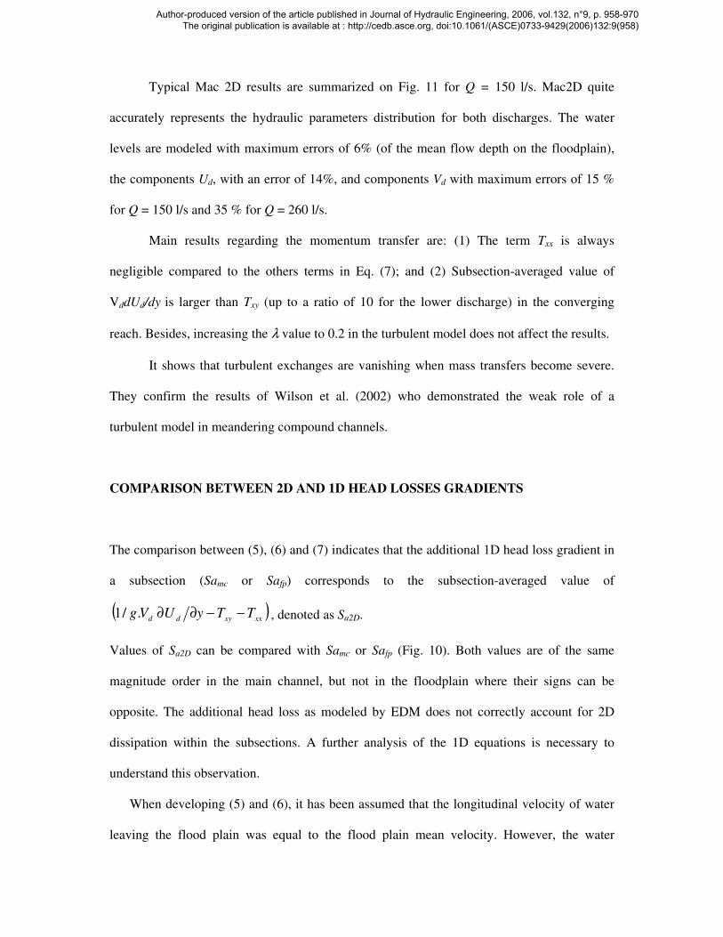
COMPARISON BETWEEN 2D AND 1D HEAD LOSSES GRADIENTS

The comparison between (5), (6) and (7) indicates that the additional 1D head loss gradient in

a subsection (Samc or Safp) corresponds to the subsection-averaged value of

( )xxxydd

TTyUVg −−∂∂./1 , denoted as Sa2D.

Values of Sa2D can be compared with Samc or Safp (Fig. 10). Both values are of the same

magnitude order in the main channel, but not in the floodplain where their signs can be

opposite. The additional head loss as modeled by EDM does not correctly account for 2D

dissipation within the subsections. A further analysis of the 1D equations is necessary to

understand this observation.

When developing (5) and (6), it has been assumed that the longitudinal velocity of water

leaving the flood plain was equal to the flood plain mean velocity. However, the water


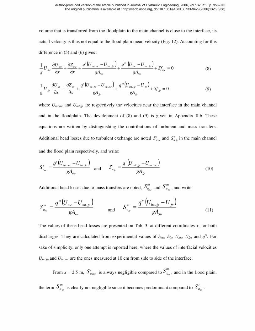
volume that is transferred from the floodplain to the main channel is close to the interface, its

actual velocity is thus not equal to the flood plain mean velocity (Fig. 12). Accounting for this

difference in (5) and (6) gives :

( ) ( )0

1 .int.int.int=+

−+

−+

∂

∂+

∂

∂mc

mc

fpmc

m

mc

fpmc

t

mcmc

mcSf

gA

UUq

gA

UUq

x

Z

x

UU

g (8)

( ) ( )0

1 .int.int.int=+

−+

−+

∂

∂+

∂

∂fp

fp

fpfp

m

fp

mcfp

t

fpfp

fpSf

gA

UUq

gA

UUq

x

Z

x

UU

g (9)

where Uint.mc and Uint.fp are respectively the velocities near the interface in the main channel

and in the floodplain. The development of (8) and (9) is given in Appendix II.b. These

equations are written by distinguishing the contributions of turbulent and mass transfers.

Additional head losses due to turbulent exchange are noted mc

t

aS and fp

t

aS in the main channel

and the flood plain respectively, and write:

( )mc

fpmc

t

t

agA

UUqS

mc

.int.int−

= and

( )fp

mcfp

t

t

agA

UUqS

fp

.int.int−

= (10)

Additional head losses due to mass transfers are noted, m

amcS and

m

a fpS , and write:

( )mc

fpmc

m

m

agA

UUqS

mc

.int−

= and

( )fp

fpfp

m

m

agA

UUqS

fp

−=

.int

(11)

The values of these head losses are presented on Tab. 3, at different coordinates x, for both

discharges. They are calculated from experimental values of hmc, hfp, Umc, Ufp, and qm. For

sake of simplicity, only one attempt is reported here, where the values of interfacial velocities

Uint.fp and Uint.mc are the ones measured at 10 cm from side to side of the interface.

From x = 2.5 m, mc

t

aS is always negligible compared tom

amcS , and in the flood plain,

the term m

a fpS is clearly not negligible since it becomes predominant compared to

t

a fpS .


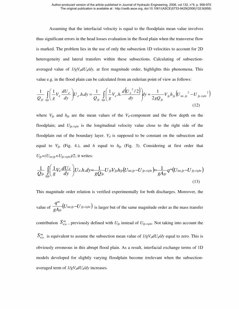
Assuming that the interfacial velocity is equal to the floodplain mean value involves

thus significant errors in the head losses evaluation in the flood plain when the transverse flow

is marked. The problem lies in the use of only the subsection 1D velocities to account for 2D

heterogeneity and lateral transfers within these subsections. Calculating of subsection-

averaged value of 1/gVddUd/dy, at first magnitude order, highlights this phenomena. This

value e.g. in the flood plain can be calculated from an eulerian point of view as follows:

( ) ( )2

.

2

.int

2

2

12/..

11...

11rightfpfpfpfp

fpAfp

d

d

fp

d

Afp

d

d

fp

UUhVgQ

dydy

UdhV

gQdyhU

dy

dUV

gQ−≈

=

∫∫

(12)

where Vfp and hfp are the mean values of the Vd-component and the flow depth on the

floodplain; and Ufp.right is the longitudinal velocity value close to the right side of the

floodplain out of the boundary layer. Vd is supposed to be constant on the subsection and

equal to Vfp (Fig. 4.), and h equal to hfp (Fig. 3). Considering at first order that

Ufp=(Uint.fp+Ufp.right)/2, it writes:

( ) ( )rightfpfpm

fprightfpfpfpfpfp

fpd

Afp

dd

fpUUq

gAUUhVU

gQdyhU

dydUV

gQ..int..int

11...11 −=−≈

∫

(13)

This magnitude order relation is verified experimentally for both discharges. Moreover, the

value of ( )rightfpfpfp

m

UUgA

q..int − is larger but of the same magnitude order as the mass transfer

contribution ma fp

S , previously defined with Ufp instead of Ufp.right. Not taking into account the

ma fp

S is equivalent to assume the subsection mean value of 1/gVddUd/dy equal to zero. This is

obviously erroneous in this abrupt flood plain. As a result, interfacial exchange terms of 1D

models developed for slightly varying floodplain become irrelevant when the subsection-

averaged term of 1/gVddUd/dy increases.


Considering interfacial velocities leads to new values of mcaS = mc

t

aS +m

amcS and of

fpaS =

t

a fpS +

m

a fpS that are reported on Fig. 10. Their sign and their magnitude order are now similar

to the ones of 2D additional head losses. Thus, one way to limit errors of 1D approaches

would be to find a suitable way to forecast interfacial velocities in both subsections.

Eventually, the comparison between (5), (6) and (7) assumes that the 1D bed friction

slope Sf, and the 2D one, Sfx, are equal. Sf is computed using experimental 1D values, and Sfx is

given by Mac2D. Fig. 13 does not show significant discrepancy between these friction slopes,

although the evaluation of Sfx partly encompasses the value of the v-component of velocity.

1D COMPUTATIONS WITH NUMERICAL PROGRAMS

Several possible weaknesses of 1D approaches in the abrupt contraction case have already

been identified: (1) the modelling of interfacial mass transfer and the associated momentum;

and (2) the assumption of a unique water level across the section in the last part of the studied

reach. Additional errors can also arise from the 1D numerical programs, due e.g. to the choice

of the equations, or to the setting of the boundary conditions. Three 1D programs were tested

for this configuration: (1) Hec-RAS, from the USACE; (2) Talweg-Fluvia, developed by the

Cemagref, Lyon, France; and (3) Axeriv, developed by the Université Catholique de Louvain,

Louvain-la-Neuve, Belgium. All these programs predict water profiles, discharge distribution

between subsections and subsection-averaged velocities.

Solved equations

Talweg-Fluvia (TF) accounts for the momentum transfer in compound channels

through the Debord formula. It solves the 1D-momentum equation on the whole cross-section:


f

tot

tot SgA

Q

xAx

Z−=

∂

∂+

∂

∂2

1β (14)

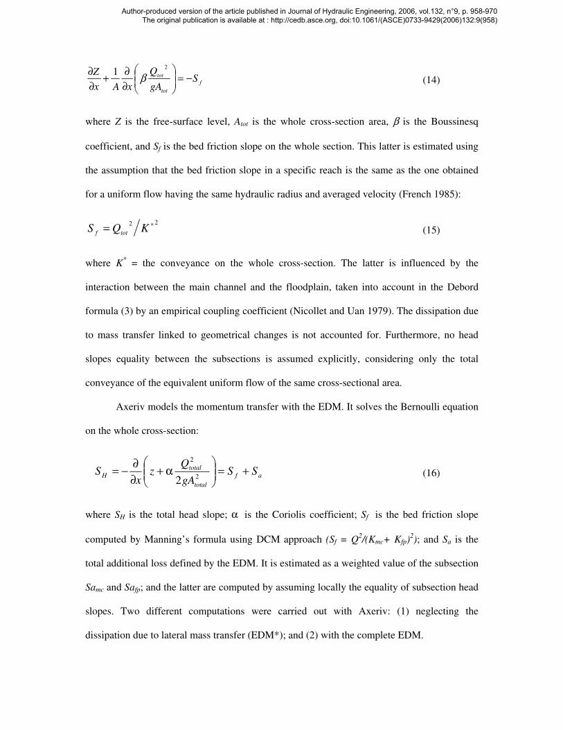
where Z is the free-surface level, Atot is the whole cross-section area, β is the Boussinesq

coefficient, and Sf is the bed friction slope on the whole section. This latter is estimated using

the assumption that the bed friction slope in a specific reach is the same as the one obtained

for a uniform flow having the same hydraulic radius and averaged velocity (French 1985):

22 ∗= KQStotf (15)

where K* = the conveyance on the whole cross-section. The latter is influenced by the

interaction between the main channel and the floodplain, taken into account in the Debord

formula (3) by an empirical coupling coefficient (Nicollet and Uan 1979). The dissipation due

to mass transfer linked to geometrical changes is not accounted for. Furthermore, no head

slopes equality between the subsections is assumed explicitly, considering only the total

conveyance of the equivalent uniform flow of the same cross-sectional area.

Axeriv models the momentum transfer with the EDM. It solves the Bernoulli equation

on the whole cross-section:

af

total

total

H SSgA

Qz

xS +=

α+

∂

∂−=

2

2

2 (16)

where SH is the total head slope; α is the Coriolis coefficient; Sf is the bed friction slope

computed by Manning’s formula using DCM approach (Sf = Q2/(Kmc+ Kfp)

2); and Sa is the

total additional loss defined by the EDM. It is estimated as a weighted value of the subsection

Samc and Safp; and the latter are computed by assuming locally the equality of subsection head

slopes. Two different computations were carried out with Axeriv: (1) neglecting the

dissipation due to lateral mass transfer (EDM*); and (2) with the complete EDM.


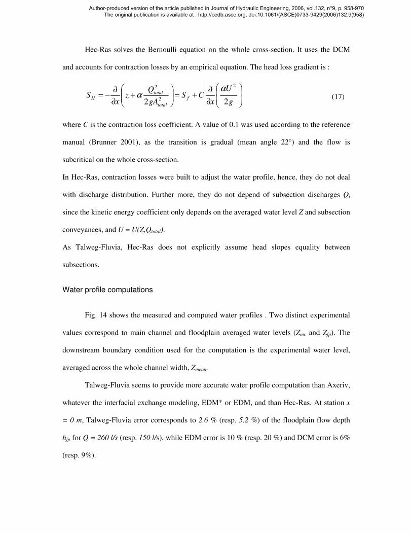
Hec-Ras solves the Bernoulli equation on the whole cross-section. It uses the DCM

and accounts for contraction losses by an empirical equation. The head loss gradient is :

∂

∂+=

+

∂

∂−=

g

U

xCS

gA

Qz

xS f

total

total

H22

2

2

2 αα (17)

where C is the contraction loss coefficient. A value of 0.1 was used according to the reference

manual (Brunner 2001), as the transition is gradual (mean angle 22°) and the flow is

subcritical on the whole cross-section.

In Hec-Ras, contraction losses were built to adjust the water profile, hence, they do not deal

with discharge distribution. Further more, they do not depend of subsection discharges Qi

since the kinetic energy coefficient only depends on the averaged water level Z and subsection

conveyances, and U = U(Z,Qtotal).

As Talweg-Fluvia, Hec-Ras does not explicitly assume head slopes equality between

subsections.

Water profile computations

Fig. 14 shows the measured and computed water profiles . Two distinct experimental

values correspond to main channel and floodplain averaged water levels (Zmc and Zfp). The

downstream boundary condition used for the computation is the experimental water level,

averaged across the whole channel width, Zmean.

Talweg-Fluvia seems to provide more accurate water profile computation than Axeriv,

whatever the interfacial exchange modeling, EDM* or EDM, and than Hec-Ras. At station x

= 0 m, Talweg-Fluvia error corresponds to 2.6 % (resp. 5.2 %) of the floodplain flow depth

hfp for Q = 260 l/s (resp. 150 l/s), while EDM error is 10 % (resp. 20 %) and DCM error is 6%

(resp. 9%).


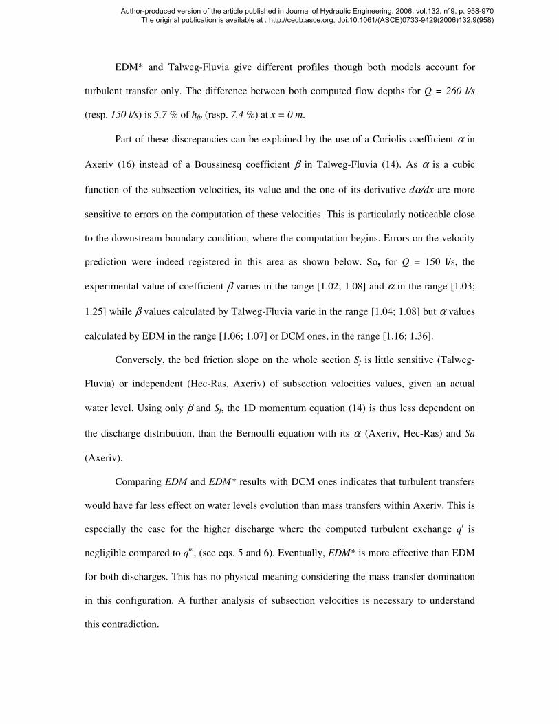
EDM* and Talweg-Fluvia give different profiles though both models account for

turbulent transfer only. The difference between both computed flow depths for Q = 260 l/s

(resp. 150 l/s) is 5.7 % of hfp (resp. 7.4 %) at x = 0 m.

Part of these discrepancies can be explained by the use of a Coriolis coefficient α in

Axeriv (16) instead of a Boussinesq coefficient β in Talweg-Fluvia (14). As α is a cubic

function of the subsection velocities, its value and the one of its derivative dα/dx are more

sensitive to errors on the computation of these velocities. This is particularly noticeable close

to the downstream boundary condition, where the computation begins. Errors on the velocity

prediction were indeed registered in this area as shown below. So, for Q = 150 l/s, the

experimental value of coefficient β varies in the range [1.02; 1.08] and α in the range [1.03;

1.25] while β values calculated by Talweg-Fluvia varie in the range [1.04; 1.08] but α values

calculated by EDM in the range [1.06; 1.07] or DCM ones, in the range [1.16; 1.36].

Conversely, the bed friction slope on the whole section Sf is little sensitive (Talweg-

Fluvia) or independent (Hec-Ras, Axeriv) of subsection velocities values, given an actual

water level. Using only β and Sf, the 1D momentum equation (14) is thus less dependent on

the discharge distribution, than the Bernoulli equation with its α (Axeriv, Hec-Ras) and Sa

(Axeriv).

Comparing EDM and EDM* results with DCM ones indicates that turbulent transfers

would have far less effect on water levels evolution than mass transfers within Axeriv. This is

especially the case for the higher discharge where the computed turbulent exchange qt is

negligible compared to qm, (see eqs. 5 and 6). Eventually, EDM* is more effective than EDM

for both discharges. This has no physical meaning considering the mass transfer domination

in this configuration. A further analysis of subsection velocities is necessary to understand

this contradiction.


Subsection-averaged velocities

Computed and measured floodplain velocities are given on Fig. 15. None of the

computations reproduces correctly the evolution of velocity along the whole reach. Similar

observations are obtained for the main channel. Some results confirm the observations made

previously on the velocity distribution for equivalent uniform flows (Fig. 9): (1) DCM values

are more and more erroneous towards downstream, underlining the role of interfacial transfers

modeling; (2) DCM corrections proposed by Debord (Talweg-Fluvia) and EDM* (Axeriv) are

sufficient to account for velocity gradients between subsections, from x = 0 to 2.5 m, where

mass transfers are moderate; (3) these corrections are no more satisfactory in the second part

of the reach, where the mass transfers increase, with a velocity underestimation up to 58 % for

Talweg-Fluvia at the last station.

Axeriv results obtained with the complete EDM, considering both turbulent and mass

transfers, require a more detailed analysis. At the station x = 4.5 m where the computation

starts, the velocity gradients computed by EDM and EDM* are equal, since the mass transfer

effect on the momentum is not yet taken into account. It has been shown that this gradient is

larger than the actual experimental value (Fig. 9). In the first computation step towards

upstream, the dissipation modeled in (5) and (6) by Samc and Safp is therefore overestimated.

This results in the too high water levels observed on Fig. 14. Furthermore, neglecting the term

ma fp

S related to interfacial velocity Uint.fp is already prejudicial in this step (Tab. 3). For further

computation steps towards upstream, the two sources of error on the interfacial transfers keep

on superimposing: (1) the artificial velocity gradient stemming from downstream; and (2) the

confusion between velocities close to the interface and the subsection ones. This explains the

different evolution of the experimental and the EDM computed subsection velocities.


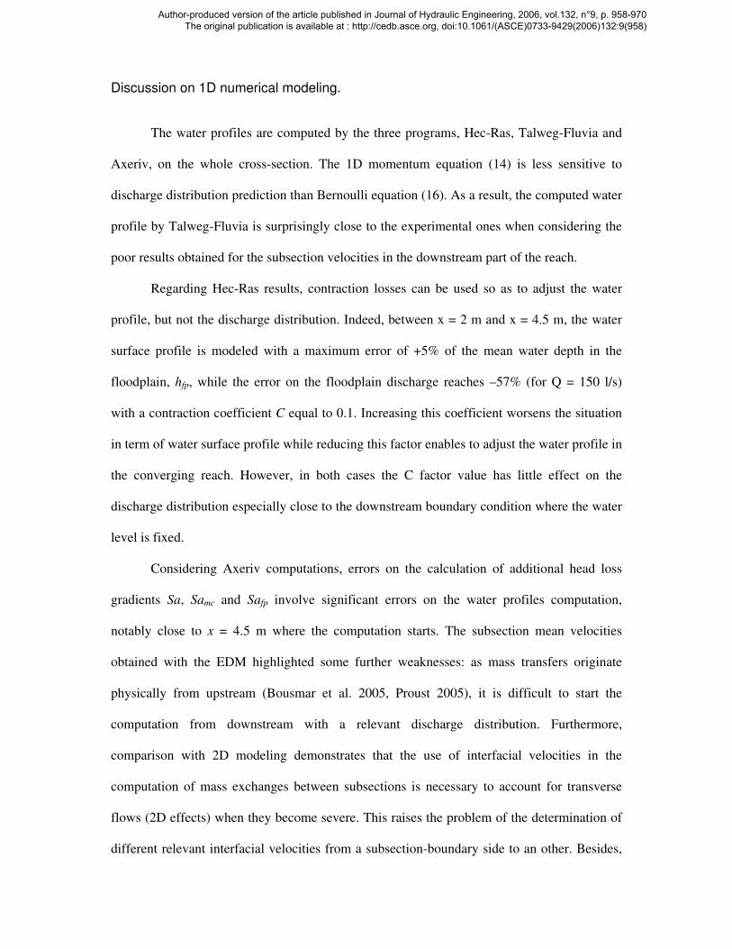
Discussion on 1D numerical modeling.

The water profiles are computed by the three programs, Hec-Ras, Talweg-Fluvia and

Axeriv, on the whole cross-section. The 1D momentum equation (14) is less sensitive to

discharge distribution prediction than Bernoulli equation (16). As a result, the computed water

profile by Talweg-Fluvia is surprisingly close to the experimental ones when considering the

poor results obtained for the subsection velocities in the downstream part of the reach.

Regarding Hec-Ras results, contraction losses can be used so as to adjust the water

profile, but not the discharge distribution. Indeed, between x = 2 m and x = 4.5 m, the water

surface profile is modeled with a maximum error of +5% of the mean water depth in the

floodplain, hfp, while the error on the floodplain discharge reaches –57% (for Q = 150 l/s)

with a contraction coefficient C equal to 0.1. Increasing this coefficient worsens the situation

in term of water surface profile while reducing this factor enables to adjust the water profile in

the converging reach. However, in both cases the C factor value has little effect on the

discharge distribution especially close to the downstream boundary condition where the water

level is fixed.

Considering Axeriv computations, errors on the calculation of additional head loss

gradients Sa, Samc and Safp involve significant errors on the water profiles computation,

notably close to x = 4.5 m where the computation starts. The subsection mean velocities

obtained with the EDM highlighted some further weaknesses: as mass transfers originate

physically from upstream (Bousmar et al. 2005, Proust 2005), it is difficult to start the

computation from downstream with a relevant discharge distribution. Furthermore,

comparison with 2D modeling demonstrates that the use of interfacial velocities in the

computation of mass exchanges between subsections is necessary to account for transverse

flows (2D effects) when they become severe. This raises the problem of the determination of

different relevant interfacial velocities from a subsection-boundary side to an other. Besides,


the subsection head slopes equality assumed by the EDM could be an other source of

discrepancies between computed and experimental values.

CONCLUSIONS

The flow in a compound channel transition reach presenting an abrupt floodplain

contraction (mean angle of 22°) has been investigated experimentally. With such a strong

contraction, a noticeable mass transfer occurs from the floodplain towards the main channel.

Specific phenomena associated to this severe mass transfer are highlighted: (1) a transverse

water surface gradient appears in the narrowest cross-section; and (2) the head evolution is

different in the main channel and in the floodplain. Besides, 2D computations are used to

evaluate the 2D head loss gradients and the relative weight of the different dissipation

sources. They show that turbulent exchanges are vanishing when mass transfer becomes

severe, as observed by Wilson et al. (2002) in meandering compound channels. Their

accuracy is satisfactory since the water surface profile and the longitudinal component Ud are

modeled with a maximum error of 6% and 12%, respectively.

Then, the relevance of three 1D numerical models developed for prismatic or slightly

non-prismatic compound channel has been analyzed. Their effectiveness is directly related to

the accuracy of the interfacial transfer modeling – notably the mass exchanges and the

associated momentum transfer – and can be worsened by assumptions such as a same head

loss gradient in the two subsections.

1D models such as Talweg-Fluvia or Axeriv with EDM* only account for turbulent

exchange between subsections. Assuming the discharge distribution is the one of the

equivalent uniform flow of same cross-section area all along the flow, they minimize error

prediction on subsection discharges by adding turbulent dissipation, which has no physical


sense in the converging part of the reach. In any case, a velocity underestimation up to 35 %

still remains for Talweg-Fluvia at the last station. Considering Hec-Ras results, errors on the

mean flow depth and mean velocity in the floodplain are 10% and 57%, respectively. The

actual discharge distribution cannot be modeled by calibrating the contraction coefficient in

Bernoulli equation. Axeriv with the complete EDM was validated for overbank flows in

symmetrically narrowing floodplains (Bousmar et al. 2004) for which, converging angles

were 3.8° or 11.3°. In this abrupt floodplain, the additional 1D head loss gradient calculated

by the EDM is less relevant, leading to error of 20% and 37% on mean flow depth and mean

velocity in the floodplain, respectively. The comparison of 2D and 1D head loss gradients

enables quantifying the role of the lateral velocity components and lateral gradient of

longitudinal velocities, which is significant in the studied configuration. 2D effects could be

integrated in the EDM by considering and computing interfacial velocities.

For the three models, assuming that the water level is equal in both beds of the same

cross-section participates to the discrepancy, with maximum error of 9% on the floodplain

mean velocity. Accordingly, erroneous results on the discharge distribution arise because of:

(1) this assumption of a unique water level in the narrowest cross-section; (2) incorrect

estimation of momentum exchange due to lateral mass transfers; (3) the assumption of

equality between head loss gradients in the two beds. Further more, a fourth source of

discrepancy was identified: the downstream boundary conditions that are imposed by current

1D models. Indeed, the 1D codes usually assume that the downstream discharge distribution

is the same as the one of the equivalent uniform flow. This assumption is not realistic and

influences the computation of lateral mass discharge in the EDM, from downstream towards

upstream. In transition reaches, a relevant calculation should consider the actual subsection

discharges in addition to the water level.


Eventually, capacities and limitations of the three different 1D codes were described.

Though they are effective in straight or slightly varied compound channel geometries

(converging angle up to 11° for the EDM), their results appear not to be relevant for a mean

angle of 22°. Accordingly, when simultaneous prediction of both water levels and mean

velocity in the flood plain is needed, e.g. for the evaluation of vulnerability in urbanized flood

plains or sediment transport in natural floodplains and for the science of habitat hydraulics,

1D models should not be used if mass transfer become severe.

However, as only one geometric configuration with two flow rates was tested, further

work should be devoted to the understanding of severe mass transfers in non-prismatic

compound channels.

ACKNOWLEDGMENTS

Experiments in CNR flume were funded by PNRH99-04 research programme. D.Bousmar,

N.Rivière and S.Proust travel costs were supported by the Tournesol programme grant

02947VM funded by EGIDE, France and CGRI, Communauté française de Belgique.


APPENDIX I. REFERENCES

Abril, J. B., and Knight, D. W. (2004). "Stage-discharge prediction for rivers in flood

applying a depth-averaged model." Journal of Hydraulic Research, 42(6), 616-629.

Ackers, P. (1991). “Hydraulic design of straight compound channels.” Rep. No. SR281, HR

Wallingford.

Ackers, P. (1992). “Hydraulic design of two-stage channels.” Proc., I.C.E., Water, Maritime

and Energy, Thomas Telford, London, 96(4), 247-257.

Bousmar, D. and Zech, Y. (1999). "Momentum transfer for practical flow computation."

Journal of Hydraulic Engineering, ASCE, 125(7), 696-706.

Bousmar, D. (2002). «Flow modelling in compound channels, momentum transfer between

main channel and prismatic or non-prismatic flood plains. » PhD-Thesis, Université

Catholique de Louvain, Louvain-la-Neuve, Belgium.

Bousmar, D., Wilkin, N., Jacquemart, J.-H. and Zech, Y. (2004), “Overbank flow in

symmetrically narrowing floodplains.” Journal of Hydraulic Engineering, ASCE, 130

(4), 305-312.

Bousmar, D., Rivière, N., Proust, S., Paquier, A., Morel, R., and Zech, Y. (2005). "Upstream

discharge distribution in compound-channel flumes." Journal of Hydraulic

Engineering, ASCE, 131(5), 408-412.

Brunner, G. W. (2001). "Hec-Ras, River Analysis system - Hydraulic Reference Manual."

USACE, Inst. for Water Resources, Hydrologic Engineering Center, Davis CA, CPD-

69.

Elliot, S. C. A. and Sellin, R. H. J. (1990). "SERC Flood channel facility : skewed flow

experiments." Journal of Hydraulic Research, Delft, The Netherlands, 28(2), 197-214.

French, R. H. (1985). “Open Channel Hydraulics.” McGraw-Hill, New –York.


Hunt, H., Brunner, G.W., and Larock, B.E., (1999). “Flow transitions in bridge backwater

analysis.” Journal of Hydraulic Engineering, ASCE, 125 (9), 981-983.

Jasem, H. K. (1990). ”Flow in two-stage channels with the main channel skewed to the flood

plain direction.” PhD Thesis, University of Glasgow, U.K.

Knight, D. W. and Demetriou, J. D. (1983). "Floodplain and main channel flow interaction."

Journal of Hydraulic Engineering, ASCE, 109(8), 1073-1092.

Knight, D. W. and Rhodes, D. G. (1994). "Velocity and boundary shear in a wide compound

duct." Journal of Hydraulic Research, Delft, The Netherlands, 32(5).

Lancastre, A., (1999). « Hydraulique générale. », Eyrolles, Paris.

Martin-Vide, J. P., Lopez-Querol, S., and Martin-Moretta, P. (2004). "Improving 1-D

modelling of open channel flow in compound channels." Proc. of the 2nd int. conf. on

fluvial hydraulics, River flow 2004, 23-25 june,, Napoly, Italy, Greco, Carravetta &

Della Morte (eds.), 415-422.

Nicollet, G. and Uan, M. (1979). "Ecoulements permanents à surface libre en lit composés."

La Houille Blanche, Grenoble, France, (1), 21-30.

Proust, S., Rivière, N., Bousmar, D., Paquier, A. and Morel, R. (2002). "Velocity

measurements in a concrete experimental channel representing a flood plain." Proc. Hydr.

Meas. and Exp. Meth., Eastes Park, Colorado, ASCE, CD-Rom.

Proust, S. (2005). “Non-uniform flows in compound channels: effect of flow-width variations

in the floodplain.” PhD-Thesis, n° 2005-ISAL-0083, INSA Lyon, Lyon, France.

Rivière, N., Proust, S., Bousmar, D., Paquier, A., Morel, R., and Zech, Y. (2002). "Relevance

of 1D flow modelling for compound channels with a converging floodplain." River

Flow 2002, Proceedings of the International Conference on Fluvail Hydraulics, 4-6

Septembre 2002, Louvain-la-Neuve, Belgium, 1, 187-195.


Rodi, W. (1980). Turbulence models and their application in hydraulics : a state of the art

review, IAHR book publication, Delft.

Sellin, R. H. J., Ervine, D. A., and Willetts, B.B. (1993). “Behaviour of meandering two-stage

channels.” Proc. Institution of Civil Engineers, Water, Maritime and Energy, 101, 99-

111.

Shiono, K. and Muto, Y. (1998). "Complex flow mechanisms in compound meandering

channels with overbank flow." Journal of Fluid Mechanics, Cambridge, England, 376,

221-226.

Shiono, K., and Knight, D. W. (1991). "Turbulent open channel flows with variable depth

across the channel." Journal of Fluid Mechanics, Cambridge, England, 222, 617-646.

Sturm, T. W., Janjua, N.S. (1994). “Clear-water scour around abutments in floodplains“.

Journal of Hydraulic Engineering, 120(8), 956-972.

Wilson, C., Bates, P. D., and Hervouet, J. M. (2002). "Comparison of turbulence models for

stage-discharge rating curve prediction in reach-scale compound channel flows using

two-dimensional finite element methods." Journal of Hydrology, 257(1-4), 42-58.

Wormleaton, P. R. and Merrett, D. J. (1990). "An improved method of the calculation for

steady uniform flow in prismatic main channel/flood plain sections." Journal of

Hydraulic Research, Delft, The Netherlands, 28(2), 157-174.

Yen, B. C. (1984). « Hydraulics of flood plains : methodology for backwater computation.”

Report Nr. 84/5 (HWV 053), Institut für wasserbau , Universität Stuttgart, Stuttgart,

Germany.

Yen, B.C., Camacho, R., Kohane, R. and Westrich, B. (1985). “Significance of flood plains in

backwater computation.” Proc. 21st Congress of IAHR, Melbourne, Australia, vol(3),

pp. 439-445.


Yen, B. C. (2002). "Open Channel Flow Resistance." Journal of Hydraulic Engineering,

ASCE, 128(1), 20-39.


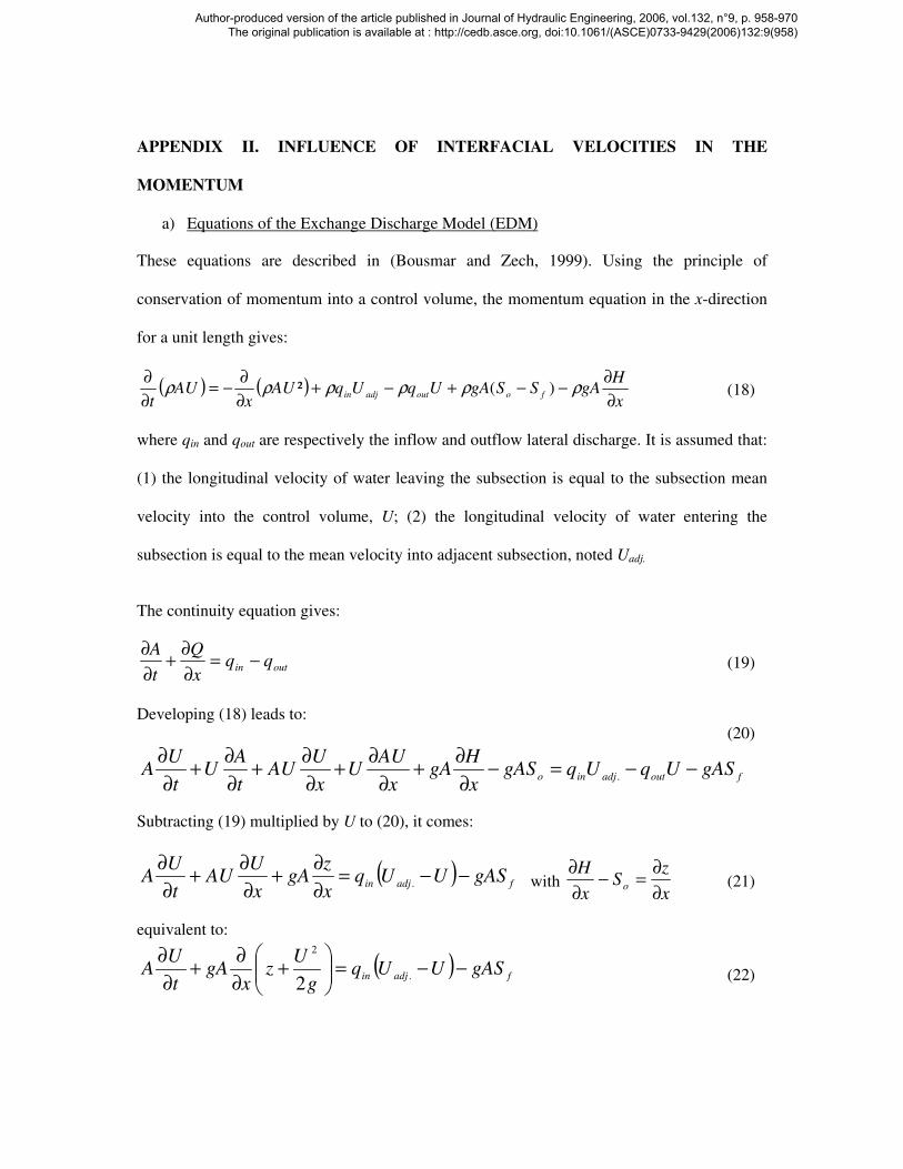
APPENDIX II. INFLUENCE OF INTERFACIAL VELOCITIES IN THE

MOMENTUM

a) Equations of the Exchange Discharge Model (EDM)

These equations are described in (Bousmar and Zech, 1999). Using the principle of

conservation of momentum into a control volume, the momentum equation in the x-direction

for a unit length gives:

( ) ( )x

HgASSgAUqUqAU

xAU

tfooutadjin

∂

∂−−+−+

∂

∂−=

∂

∂ρρρρρρ )(² (18)

where qin and qout are respectively the inflow and outflow lateral discharge. It is assumed that:

(1) the longitudinal velocity of water leaving the subsection is equal to the subsection mean

velocity into the control volume, U; (2) the longitudinal velocity of water entering the

subsection is equal to the mean velocity into adjacent subsection, noted Uadj.

The continuity equation gives:

outin qqx

Q

t

A−=

∂

∂+

∂

∂ (19)

Developing (18) leads to:

(20)

foutadjinogASUqUqgAS

x

HgA

x

AUU

x

UAU

t

AU

t

UA −−=−

∂

∂+

∂

∂+

∂

∂+

∂

∂+

∂

∂.

Subtracting (19) multiplied by U to (20), it comes:

( )fadjin

gASUUqx

zgA

x

UAU

t

UA −−=

∂

∂+

∂

∂+

∂

∂. with

x

zS

x

Ho

∂

∂=−

∂

∂ (21)

equivalent to:

( )fadjin

gASUUqg

Uz

xgA

t

UA −−=

+

∂

∂+

∂

∂.

2

2 (22)


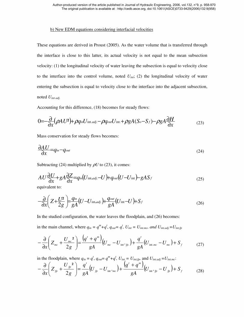
b) New EDM equations considering interfacial velocities

These equations are derived in Proust (2005). As the water volume that is transferred through

the interface is close to this latter, its actual velocity is not equal to the mean subsection

velocity: (1) the longitudinal velocity of water leaving the subsection is equal to velocity close

to the interface into the control volume, noted Uint; (2) the longitudinal velocity of water

entering the subsection is equal to velocity close to the interface into the adjacent subsection,

noted Uint.adj.

Accounting for this difference, (18) becomes for steady flows:

( )xHgASSgAUqUqAU

xfooutadjin

∂∂−−+−+

∂∂−= ρρρρρ )(²0 .int..int (23)

Mass conservation for steady flows becomes:

outin qqx

AU −=∂

∂ (24)

Subtracting (24) multiplied by ρU to (23), it comes:

( ) ( ) foutadjin gASUUqUUqxZgA

xUAU −−+−=

∂∂+

∂∂

int.int. (25)

equivalent to:

( ) ( ) fout

adjin

SUUgA

qUU

gA

q

gUZ

x+−+−=

+

∂∂− int.int.

2²

(26)

In the studied configuration, the water leaves the floodplain, and (26) becomes:

in the main channel, where qin = qm+q

t, qout= q

t, Uint = Uint.mc, and Uint.adj.=Uint.fp

( )( ) ( )fmcmc

t

fpmc

mt

mc

mcSUU

gA

qUU

gA

qq

g

UZ

x+−+−

+=

+

∂

∂−

.int.int.

2

² (27)

in the floodplain, where qin = qt, qout= q

m+q

t, Uint = Uint.fp, and Uint.adj.=Uint.mc:

( ) ( )( )ffpfp

mt

mcfp

t

fp

fpSUU

gA

qqUU

gA

q

g

UZ

x+−

++−=

+

∂

∂− ..

2

²intint (28)


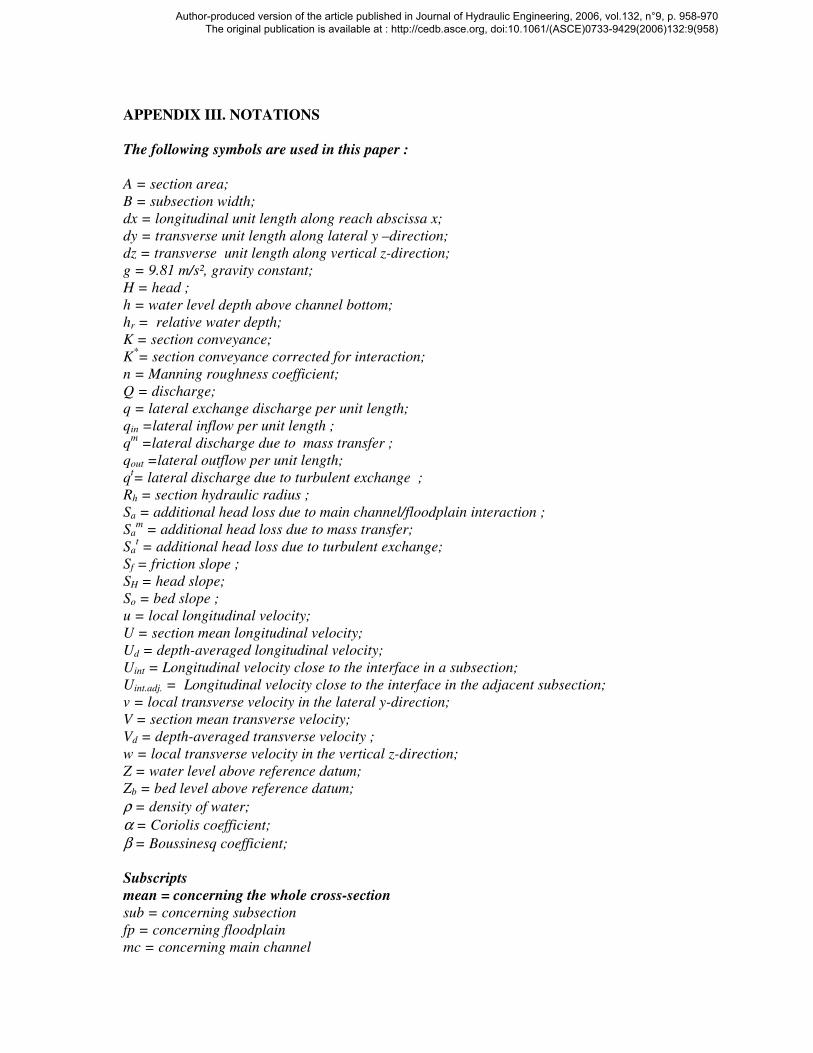
APPENDIX III. NOTATIONS

The following symbols are used in this paper :

A = section area;

B = subsection width;

dx = longitudinal unit length along reach abscissa x;

dy = transverse unit length along lateral y –direction;

dz = transverse unit length along vertical z-direction;

g = 9.81 m/s², gravity constant;

H = head ;

h = water level depth above channel bottom;

hr = relative water depth;

K = section conveyance;

K*= section conveyance corrected for interaction;

n = Manning roughness coefficient;

Q = discharge;

q = lateral exchange discharge per unit length;

qin =lateral inflow per unit length ;

qm =lateral discharge due to mass transfer ;

qout =lateral outflow per unit length;

qt= lateral discharge due to turbulent exchange ;

Rh = section hydraulic radius ;

Sa = additional head loss due to main channel/floodplain interaction ;

Sam = additional head loss due to mass transfer;

Sat = additional head loss due to turbulent exchange;

Sf = friction slope ;

SH = head slope;

So = bed slope ;

u = local longitudinal velocity;

U = section mean longitudinal velocity;

Ud = depth-averaged longitudinal velocity;

Uint = Longitudinal velocity close to the interface in a subsection;

Uint.adj. = Longitudinal velocity close to the interface in the adjacent subsection;

v = local transverse velocity in the lateral y-direction;

V = section mean transverse velocity;

Vd = depth-averaged transverse velocity ;

w = local transverse velocity in the vertical z-direction;

Z = water level above reference datum;

Zb = bed level above reference datum;

ρ = density of water;

α = Coriolis coefficient;

β = Boussinesq coefficient;

Subscripts

mean = concerning the whole cross-section

sub = concerning subsection

fp = concerning floodplain

mc = concerning main channel


List of figure captions

Fig. 1. Compound channel flume of the Compagnie Nationale du Rhône (CNR)

Fig. 2. Experimental set-up scheme

Fig. 3. Lateral profiles of water levels - Q = 260 l/s

Fig. 4. Lateral distributions of depth-averaged velocities: (a) longitudinal component Ud; (b)

transverse component, Vd.

Fig. 5. Velocities field in the vertical plane x = 3.5 m – Q = 260 l/s

Fig. 6. Velocities field measured near the bottom (0.2 hmc) and the surface - Q = 260 l/s.

Fig. 7. Floodplain discharge as percentage of total discharge – calculations against data.

Fig. 8. Head profiles in the whole cross-section and in the subsections

Fig. 9. Evolution of the mean velocity in the floodplain

Fig. 10. Experimental 1D additional head loss gradients Sa and 2D computed ones Sa.2D in

both subsections.

Fig. 11. Distribution of velocity components, Ud, and Vd, computed by MAC 2D for Q = 150

l/s.

Fig. 12. Schematic lateral profile of longitudinal depth-averaged velocity Ud

Fig. 13. Experimental bed friction slope Sf (1D) and computed one Sfx (2D), in both

subsections

Fig. 14. Longitudinal water surface profiles – Calculation against experimental data.

Fig. 15. Floodplain velocity profiles – Calculation against experimental data.


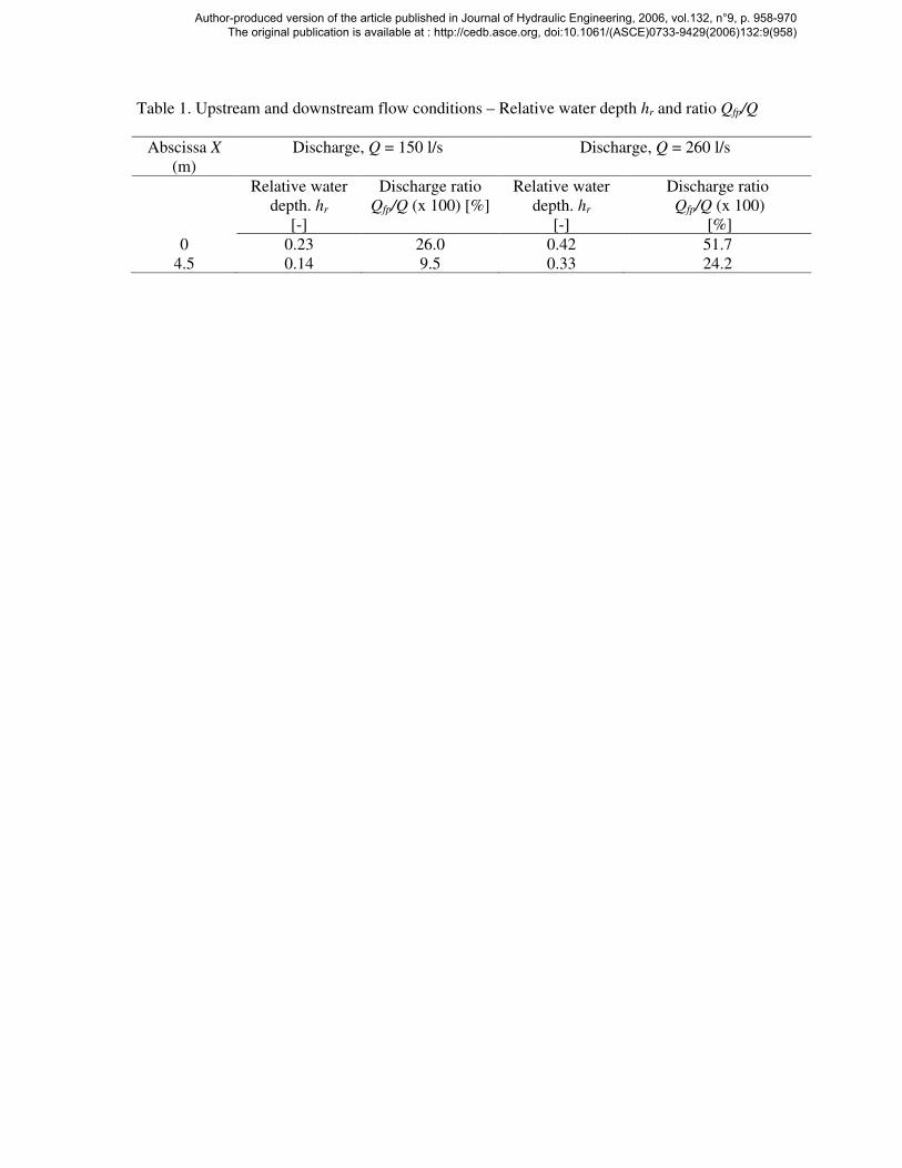
Table 1. Upstream and downstream flow conditions – Relative water depth hr and ratio Qfp/Q

Abscissa X

(m)

Discharge, Q = 150 l/s Discharge, Q = 260 l/s

Relative water

depth. hr

[-]

Discharge ratio

Qfp/Q (x 100) [%]

Relative water

depth. hr

[-]

Discharge ratio

Qfp/Q (x 100)

[%]

0 0.23 26.0 0.42 51.7

4.5 0.14 9.5 0.33 24.2


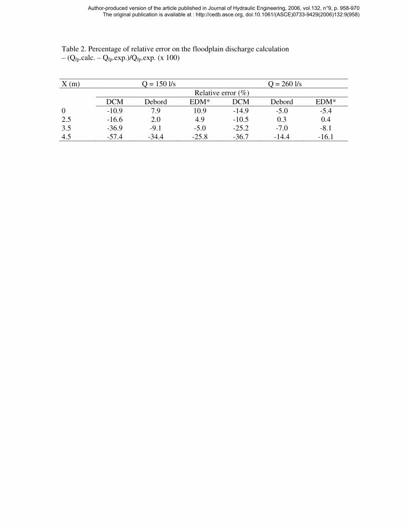
Table 2. Percentage of relative error on the floodplain discharge calculation

– (Qfp.calc. – Qfp.exp.)/Qfp.exp. (x 100)

X (m) Q = 150 l/s Q = 260 l/s

Relative error (%)

DCM Debord EDM* DCM Debord EDM*

0 -10.9 7.9 10.9 -14.9 -5.0 -5.4

2.5 -16.6 2.0 4.9 -10.5 0.3 0.4

3.5 -36.9 -9.1 -5.0 -25.2 -7.0 -8.1

4.5 -57.4 -34.4 -25.8 -36.7 -14.4 -16.1


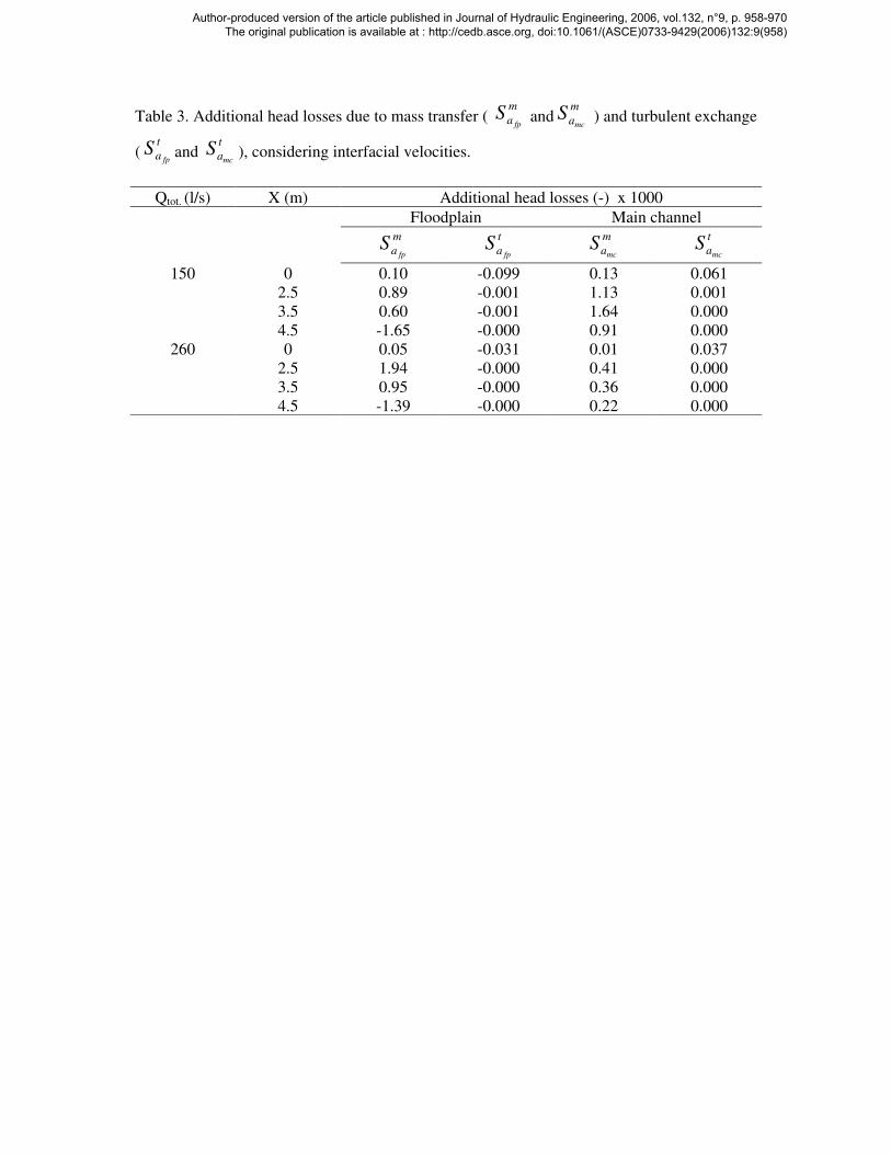
Table 3. Additional head losses due to mass transfer ( m

a fpS and

m

amcS ) and turbulent exchange

(t

a fpS and

t

amcS ), considering interfacial velocities.

Qtot. (l/s) X (m) Additional head losses (-) x 1000

Floodplain Main channel m

a fpS

t

a fpS

m

amcS

t

amcS

150 0 0.10 -0.099 0.13 0.061

2.5 0.89 -0.001 1.13 0.001

3.5 0.60 -0.001 1.64 0.000

4.5 -1.65 -0.000 0.91 0.000

260 0 0.05 -0.031 0.01 0.037

2.5 1.94 -0.000 0.41 0.000

3.5 0.95 -0.000 0.36 0.000

4.5 -1.39 -0.000 0.22 0.000


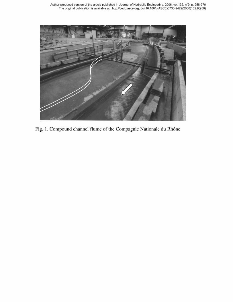
Fig. 1. Compound channel flume of the Compagnie Nationale du Rhône


x

y

Bmc=0.7m

Bfp=2.17m

0.16m

Fixed point gaugex=-0.9m

x=2.1m x=6.35m

grillage bufferWeir crestMeasuring device

Inclined gate

Channelcross section

gv

gv

Slope : 0.0019

Stillingbasin

x=09.4 m-3.6 m

2/3 Bfp

main channel

flood plain

FIG. 2. Experimental setup scheme


22

23

24

25

26

27

28

29

0.0 0.5 1.0 1.5 2.0 2.5 3.0

Y [m]

Wate

r le

vel Z

[cm

]

X = 0 m

X = 2.5 m

X = 3.5 m

X = 4.5 m

Q = 260 l/s

FIG. 3. Lateral profiles of water levels - Q = 260 l/s


Q = 150 l/s

0.0

0.2

0.4

0.6

0.8

1.0

1.2

0.0 0.5 1.0 1.5 2.0 2.5 3.0Y [m]

Velo

cit

y [

m/s

]

X = 0 m

X = 2.5 m

X = 3.5 m

X = 4.5 m

(a)

Q = 150 l/s

-0.05

0.00

0.05

0.10

0.15

0.20

0.25

0.30

0.0 0.5 1.0 1.5 2.0 2.5 3.0

Y [m]

Velo

cit

y [

m/s

]

X = 0 m

X = 2.5 m

X = 3.5 m

X = 4.5 m

(b)

Q = 260 l/s

0.0

0.2

0.4

0.6

0.8

1.0

1.2

0.0 0.5 1.0 1.5 2.0 2.5 3.0Y [m]

Velo

cit

y [

m/s

]

X = 0 m

X = 2.5 m

X = 3.5 m

X = 4.5 m

(a)

Q = 260 l/s

-0.05

0.00

0.05

0.10

0.15

0.20

0.25

0.30

0.0 0.5 1.0 1.5 2.0 2.5 3.0

Y [m]

Velo

cit

y [

m/s

]

X = 0 m

X = 2.5 m

X = 3.5 m

X = 4.5 m

(b)

FIG. 4 – Lateral distributions of depth-averaged velocities: (a) longitudinal

component Ud and (b) transverse component, Vd.


[m]

Z[m

]

[m]

Z[m

]

10 cm/s

FIG. 5 - Velocities field in the vertical plane x = 3.5 m – Q = 260 l/s


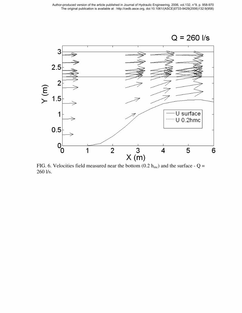
FIG. 6. Velocities field measured near the bottom (0.2 hmc) and the surface - Q =

260 l/s.


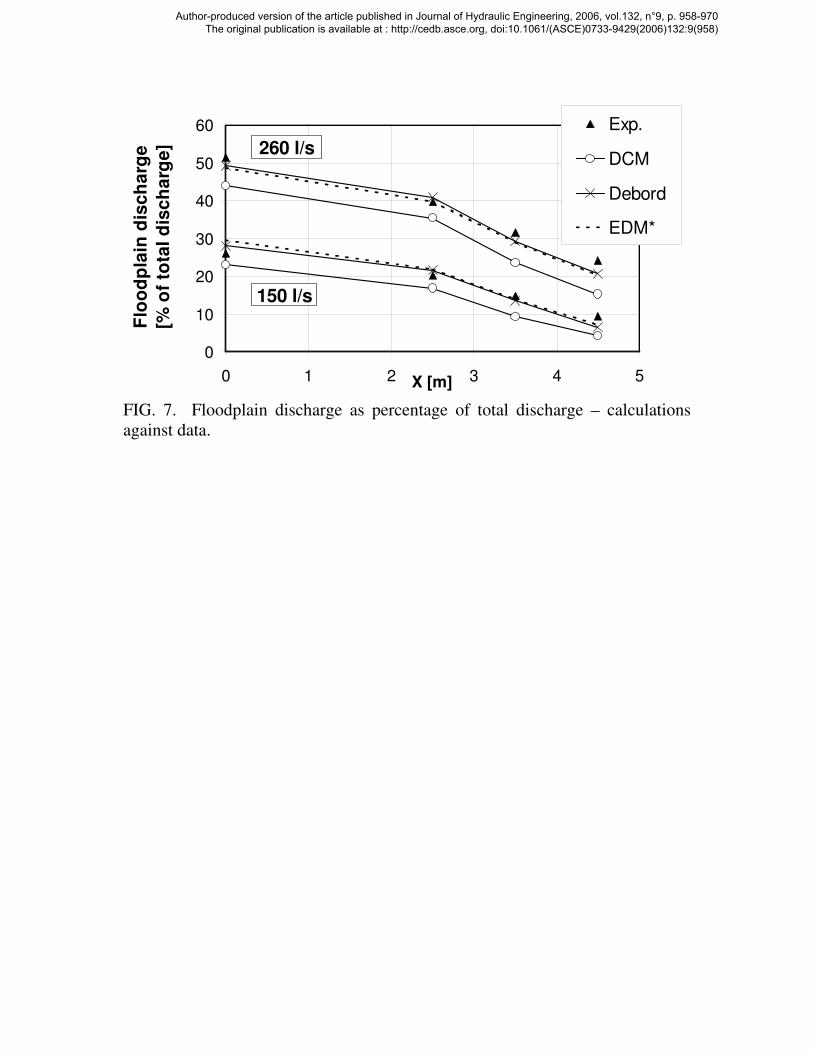
0

10

20

30

40

50

60

0 1 2 3 4 5X [m]

Flo

od

pla

in d

isc

ha

rge

[% o

f to

tal

dis

ch

arg

e]

Exp.

DCM

Debord

EDM*

260 l/s

150 l/s

FIG. 7. Floodplain discharge as percentage of total discharge – calculations

against data.


150 l/s

0.210

0.220

0.230

0.240

0.250

0 1 2 3 4 5X [m]

He

ad

[m

]

0.290

0.295

0.300

0.305

0.310

0 1 2 3 4 5X [m]

Head

[m

]

260 l/s

Whole section (u²+v²) Whole section (u) Floodplain Main channel Bed slope

FIG. 8. Head profiles in the whole cross-section and in the subsections


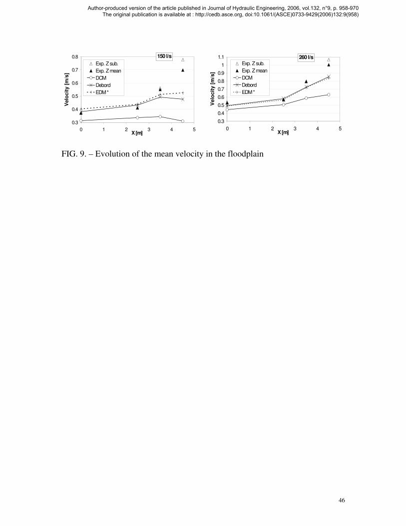
46

0.3

0.4

0.5

0.6

0.7

0.8

0 1 2 3 4 5X [m]

Velo

cit

y [

m/s

]Exp. Z sub.

Exp. Z mean

DCM

Debord

EDM *

150 l/s

0.3

0.4

0.5

0.6

0.7

0.8

0.9

1

1.1

0 1 2 3 4 5X [m]

Velo

cit

y [

m/s

]

Exp. Z sub.

Exp. Z mean

DCM

Debord

EDM *

260 l/s

FIG. 9. – Evolution of the mean velocity in the floodplain


47

150 l/s

-2

-1

0

1

2

3

0 1 2 3 4X [m]

He

ad

lo

ss

gra

die

nt

(x1

00

0)

[-]

260 l/s

-3

-2

-1

0

1

2

3

4

5

0 1 2 3 4X [m]

He

ad

lo

ss

gra

die

nt

(x1

00

0)

[-]

MC 2D MC1D MC 1D Uint FP 2D FP1D FP 1D Uint

FIG. 10 – Experimental 1D additional head loss gradients Sa and 2D computed

ones Sa.2D in both subsections.


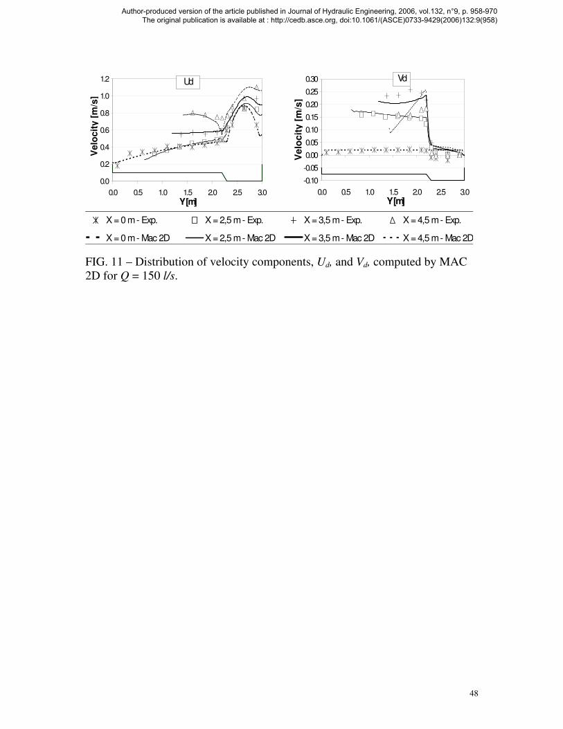
48

0.0

0.2

0.4

0.6

0.8

1.0

1.2

0.0 0.5 1.0 1.5 2.0 2.5 3.0

Y [m]

Ve

loc

ity

[m

/s]

Ud

-0.10

-0.05

0.00

0.05

0.10

0.15

0.20

0.25

0.30

0.0 0.5 1.0 1.5 2.0 2.5 3.0Y [m]

Ve

loc

ity

[m

/s]

Vd

X = 0 m - Exp. X = 2,5 m - Exp. X = 3,5 m - Exp. X = 4,5 m - Exp.

X = 0 m - Mac 2D X = 2,5 m - Mac 2D X = 3,5 m - Mac 2D X = 4,5 m - Mac 2D

FIG. 11 – Distribution of velocity components, Ud, and Vd, computed by MAC

2D for Q = 150 l/s.


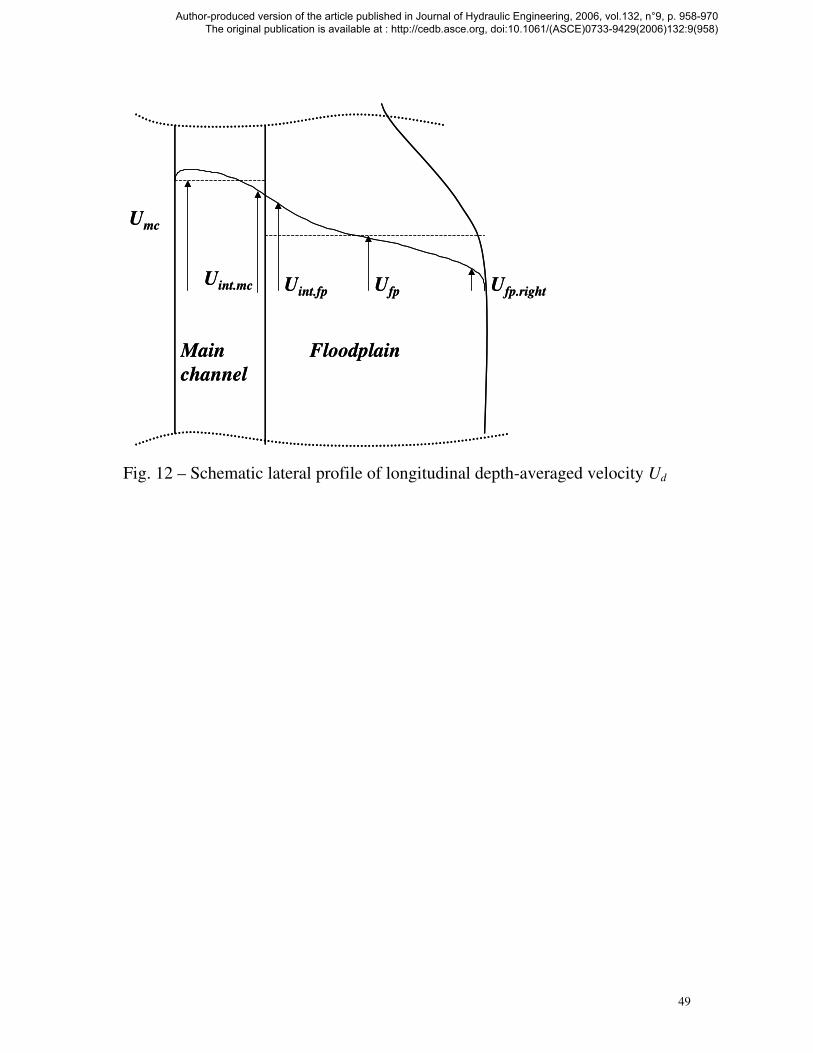
49

Main

channel

Floodplain

Umc

UfpUint.fp Ufp.rightUint.mc

Main

channel

Floodplain

Umc

UfpUint.fp Ufp.rightUint.mc

Fig. 12 – Schematic lateral profile of longitudinal depth-averaged velocity Ud


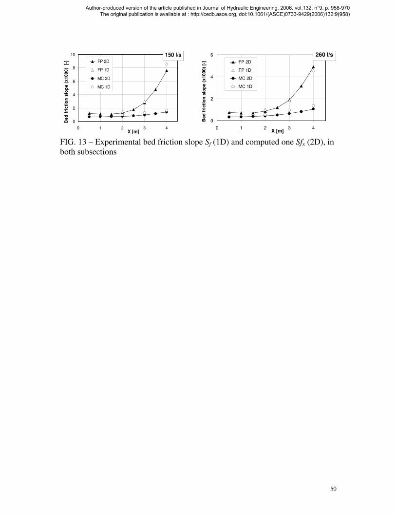
50

0

2

4

6

8

10

0 1 2 3 4X [m]

Be

d f

ric

tio

n s

lop

e (

x1

00

0)

[-] FP 2D

FP 1D

MC 2D

MC 1D

150 l/s

0

2

4

6

0 1 2 3 4X [m]

Bed

fri

cti

on

slo

pe (

x1000)

[-] FP 2D

FP 1D

MC 2D

MC 1D

260 l/s

FIG. 13 – Experimental bed friction slope Sf (1D) and computed one Sfx (2D), in

both subsections


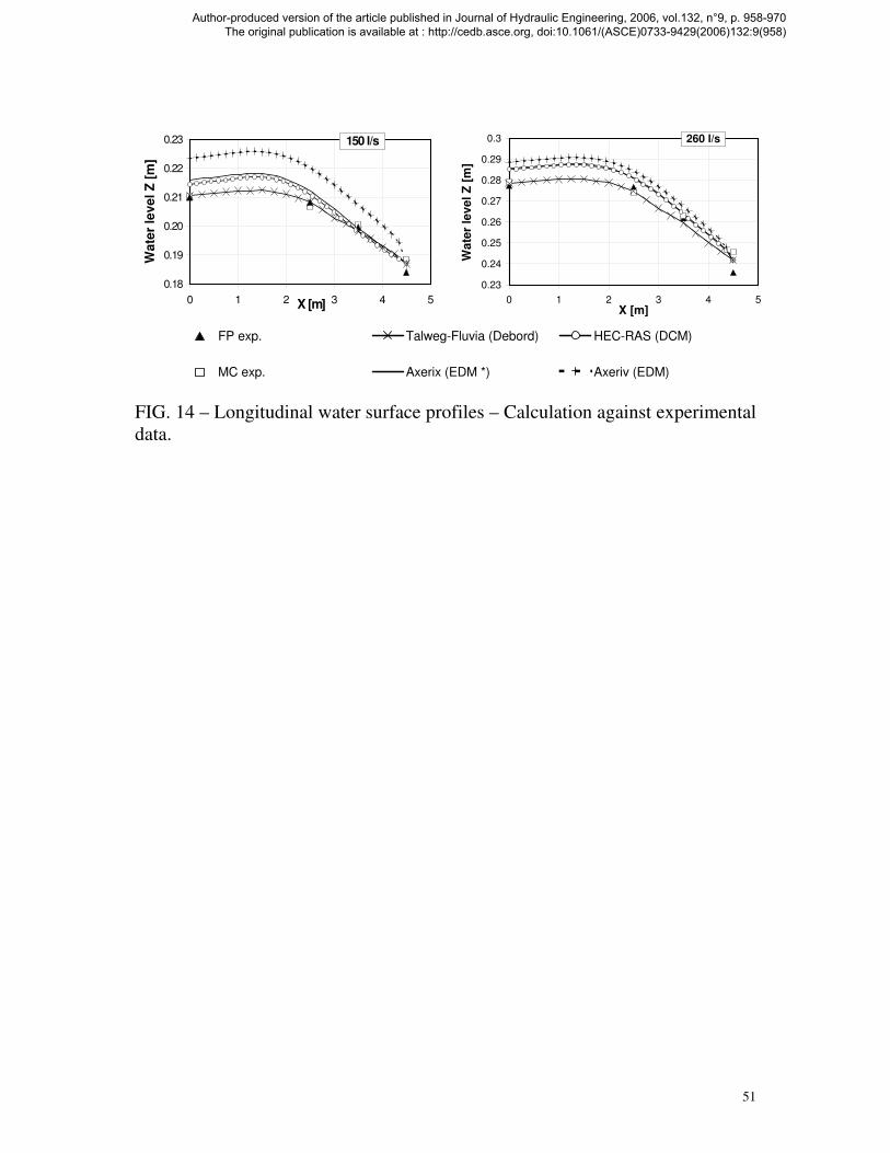
51

0.18

0.19

0.20

0.21

0.22

0.23

0 1 2 3 4 5X [m]

Wa

ter

lev

el Z

[m

]150 l/s

0.23

0.24

0.25

0.26

0.27

0.28

0.29

0.3

0 1 2 3 4 5X [m]

Wate

r le

vel

Z [

m]

260 l/s

FP exp. Talweg-Fluvia (Debord) HEC-RAS (DCM)

MC exp. Axerix (EDM *) Axeriv (EDM)

FIG. 14 – Longitudinal water surface profiles – Calculation against experimental

data.


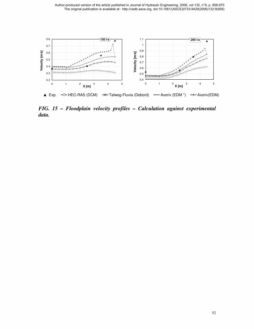
52

0.2

0.3

0.4

0.5

0.6

0.7

0.8

0 1 2 3 4 5X [m]

Ve

loc

ity

[m

/s]

150 l/s

0.4

0.5

0.6

0.7

0.8

0.9

1

1.1

0 1 2 3 4 5X [m]

Ve

loc

ity

[m

/s]

260 l/s

Exp. HEC-RAS (DCM) Talweg-Fluvia (Debord) Axeriv (EDM *) Axeriv(EDM)

FIG. 15 – Floodplain velocity profiles – Calculation against experimental

data.


Documents

Flow in compound channel with abrupt floodplain contraction