first published online 18 December 2009, doi: 10.1098/rsif.2009.04767 2010 J. R. Soc. Interface H. Baek, M. V. Jayaraman, P. D. Richardson and G. E. Karniadakis aneurysmsFlow instability and wall shear stress variation in intracranial  

Supplementary data

l http://rsif.royalsocietypublishing.org/content/suppl/2009/12/17/rsif.2009.0476.DC1.htm

"Data Supplement"

Referenceshttp://rsif.royalsocietypublishing.org/content/7/47/967.full.html#ref-list-1

This article cites 52 articles, 8 of which can be accessed free

Subject collections

(44 articles)mathematical physics   � (284 articles)biophysics   �

(140 articles)biomedical engineering   � Articles on similar topics can be found in the following collections

Email alerting service hereright-hand corner of the article or click Receive free email alerts when new articles cite this article - sign up in the box at the top

http://rsif.royalsocietypublishing.org/subscriptions go to: J. R. Soc. InterfaceTo subscribe to

on January 27, 2014rsif.royalsocietypublishing.orgDownloaded from on January 27, 2014rsif.royalsocietypublishing.orgDownloaded from

J. R. Soc. Interface (2010) 7, 967–988

on January 27, 2014rsif.royalsocietypublishing.orgDownloaded from

*Author for c

Electronic sup10.1098/rsif.2

doi:10.1098/rsif.2009.0476Published online 18 December 2009

Received 28 OAccepted 24 N

Flow instability and wall shear stressvariation in intracranial aneurysms

H. Baek1, M. V. Jayaraman2, P. D. Richardson3

and G. E. Karniadakis1,*1Division of Applied Mathematics, 2Department of Diagnostic Imaging, Warren Alpert School

of Medicine, and 3Division of Engineering and Department of Molecular Pharmacology,Physiology, and Biotechnology, Brown University, Providence, RI 02912, USA

We investigate the flow dynamics and oscillatory behaviour of wall shear stress (WSS) vectorsin intracranial aneurysms using high resolution numerical simulations. We analyse threerepresentative patient-specific internal carotid arteries laden with aneurysms of differentcharacteristics: (i) a wide-necked saccular aneurysm, (ii) a narrower-necked saccular aneur-ysm, and (iii) a case with two adjacent saccular aneurysms. Our simulations show that thepulsatile flow in aneurysms can be subject to a hydrodynamic instability during the deceler-ating systolic phase resulting in a high-frequency oscillation in the range of 20–50 Hz, evenwhen the blood flow rate in the parent vessel is as low as 150 and 250 ml min21 for cases(iii) and (i), respectively. The flow returns to its original laminar pulsatile state near theend of diastole. When the aneurysmal flow becomes unstable, both the magnitude and thedirections of WSS vectors fluctuate at the aforementioned high frequencies. In particular,the WSS vectors around the flow impingement region exhibit significant spatio-temporalchanges in direction as well as in magnitude.

Keywords: flow instability; multiple aneurysms; spectral element method; CFD

1. INTRODUCTION

Image-based computational fluid dynamics (CFD)simulations have been used to correlate wall shearstress (WSS), pressure and other indicators with theformation and growth of an aneurysm (Tateshimaet al. 2003; Cebral et al. 2005a; Torii et al. 2006;Chatziprodromou et al. 2007; Sforza et al. 2009). Inparticular, impingement zones and areas of high WSShave been correlated with aneurysm formation,growth in size, or rupture (Cebral et al. 2009). It hasbeen argued that blebs, ‘blisters on the aneurysmwall’, form in high WSS regions where the flow impingesinto aneurysms (Cebral et al. 2007). Some authors(Boussel et al. 2008; Jou et al. 2008) claim that aneur-ysms tend to grow at an area where the endotheliallayer is subject to abnormally low WSS. Hence, theability to identify these critical locations in aneurysms,i.e. abnormally high or low WSS regions and impinge-ment locations, would have significant implications fortreatment.

Flow impingement regions inside aneurysms arereported to have a particular pattern of WSS/pressuredistribution. The apex of a flow impingement area,i.e. the local region of flow stagnation, is characterizedby low WSS and higher static pressure, and is sur-rounded by a band of higher WSS and WSS gradient

orrespondence (gk@dam.brown.edu).

plementary material is available at http://dx.doi.org/009.0476 or via http://rsif.royalsocietypublishing.org.

ctober 2009ovember 2009 967

(Szymanski et al. 2008). An experimental study of animpingement area (Meng et al. 2007) showed thatdestructive remodelling involving loss of smoothmuscle cells occurs at the region of high WSS andWSS gradient where the flow accelerates. Also, a moresensitive response of endothelial cells to turbulent oscil-latory shear rather than to laminar and steady shearhas been demonstrated experimentally (Moore et al.1994; Malek et al. 1999; Meng et al. 2007). Therefore,it seems important to understand the dynamicoscillatory behaviour of WSS vectors in the impinge-ment (stagnation) locations. To this end, weinvestigate systematically the oscillatory behaviour ofWSS vectors inside an aneurysm and the flow instabil-ity due to the presence of an aneurysm at the posteriorcommunicating artery (PCoA) origin.

Intraoperative Doppler recording of Steiger & Reulen(1986) showed flow fluctuations in the aneurysms of sixpatients out of 12. Spectra calculated from the parentvessel’s recordings did not show peaks except from thebase pulsatile flow while spectra of the data from theaneurysms displayed several small peaks between 5and 20 Hz. Ferguson (1970) recorded bruits from thesacs of 10 out of 17 intracranial aneurysms during sur-gery. The murmurs from aneurysms reported bySimkins & Stehbens (1974) were associated with thefluctuating flow (Steiger et al. 1987). Sekhar &Wasserman (1984) also reported sounds from saccularaneurysms in eight of 11 patients and later they measuredsound from experimental aneurysms in the commoncarotid bifurcation of dogs (Sekhar et al. 1991).

This journal is q 2009 The Royal Society

968 Flow instability in aneurysms H. Baek et al.

on January 27, 2014rsif.royalsocietypublishing.orgDownloaded from

Cebral et al. (2005b) performed simulations to showthat ruptured aneurysms tend to have unstable (chan-ging direction of inflow jet) aneurysmal flow unlikeunruptured cases, but no further details of unstableflow are provided.1

A lateral aneurysm seems to be geometrically analo-gous to a cavity in a channel—a prototype flow whichhas been studied extensively. For the simplest cavitygeometries, a streamline departing from the surface onthe upstream edge of a rectangular cavity reattachesat or near the downstream edge of the cavity asdescribed by Batchelor (1956). Self-sustained oscil-lations including the cavity flow were reviewed inRockwell & Naudascher (1979). Cavity flow and itsstability were studied numerically by Ghaddar et al.(1986). In aneurysms in cerebral arteries, owing to theeffects of complicated geometry, we expect to find dis-tinct regions of inflow and outflow at the mouths ofwide-necked aneurysms. Such pattern of inflow and out-flow may create inflection (change of curvature) of thevelocity profile, which is the classic Rayleigh conditionfor instability (Drazin & Reid 1981). This, in fact, wasfirst hypothesized by Lighthill (1975). Hence, weexpect the instability to develop, probably only transi-ently because of the pulsatile nature of the blood flow,manifesting itself through velocity fluctuations of adistinctly higher frequency than the cardiac pulse.

Stability of pulsatile flow has been studied experimen-tally and numerically (Nerem et al. 1972; Einav &Sokolov 1993; Straatman et al. 2002; Blackburn &Sherwin 2007). Experimental study of flow in a straightpipe by Einav & Sokolov (1993) showed that pulsatileflows become ‘turbulent’ during the deceleration phaseof oscillation at Reynolds number around 2000.Straatman et al. (2002) performed a linear stabilityanalysis for plane pulsatile Poiseuille flow showing thatpulsation may trigger instabilities. Nerem et al. (1972)measured velocity in the aorta of dogs and reportedtransition to turbulence at the end of systole.

CFD simulations in the carotid stenosis (Fischeret al. 2007; Lee et al. 2008; Grinberg et al. 2009) wereperformed and intermittent turbulence during thedecelerating systole was reported. However, the currentwork seems to be the first numerical study to reportflow instability in aneurysms. Specifically we considerpatient-specific geometries showing the spectra offluctuating velocity inside aneurysms as well as timetraces of WSS vectors on the aneurysm walls underpulsatile flow with volumetric flow rate (VFR) of150–400 ml min21 in the internal carotid artery(ICA). Through a series of simulations, we report thataneurysmal flows may become unstable during thedeceleration phase. We also aim to understand thedistribution of WSS and its directional changes inaneurysms during the instability period.

In the following, we first present details of the geo-metric models and the simulation parameters in §2and subsequently results of simulations in §3. We dis-cuss findings and limitations of this study in §4

1In these simulations, about 200 time steps per cardiac cycler wereused. Hence, possible temporal fluctuations were suppressed(J. R. Cebral 2009, personal communication).

J. R. Soc. Interface (2010)

followed by conclusions in §5. In appendix A, we presentsensitivity studies, specifically: (i) a systematic resol-ution study and (ii) the effect of outflow boundaryconditions on the velocity fluctuations.

2. METHODS

In this study, we analyse three representative vesselgeometries harbouring aneurysms with different charac-teristics selected from many patients we considered. Forthis retrospective review, institutional review boardapproval was obtained. Specifically, aneurysms in thesupraclinoid ICA segment were considered; side(lateral) aneurysms are the most common and henceterminal aneurysms were not considered. Based onpatients treated endovascularly, Murayana et al.(2003) reported that approximately 40.5 per cent aresmall aneurysms (less than 10 mm maximum size)with small neck (less than 4 mm), 28.7 per cent aresmall with wide neck (more than 4 mm), 17.4 per centare large (more than 10 mm) and 6 per cent giant(more than 25 mm). In general, approximately 15–20%of patients will have multiple aneurysms. Accordingto statistics, the examples chosen in this study arerepresentative of three types of aneurysms occurringin the supraclinoid ICA: wide-necked, small-neckedand multiple aneurysms (see figure 1).

The first (patient A) has a very wide-necked aneur-ysm, resembling a fusiform aneurysm, in thesupraclinoid ICA. The second (patient B) has thePCoA harbouring a relatively narrow-necked aneurysm.The third (patient C) developed two wide-necked aneur-ysms in the supraclinoid ICA. One of them is located atthe root of the PCoA and the other one is downstreamwithin a short distance. The aneurysm of patient Band the upstream aneurysm of patient C have thePCoA branches coming out of the aneurysm wall.Hence, all chosen aneurysms are located between theophthalmic triangle and the ICA bifurcation into theanterior cerebral artery (ACA) and the middle cerebralartery (MCA) and approximately at the level of theeyes, behind the eyes and towards the middle of the head.

Images from computed tomography angiography orthree-dimensional digital subtraction angiographywere anonymized to remove any patient-specific data,and then exported in a DICOM format. The image res-olutions and more detailed information of these data areexplained in table 1. The vessel geometries were manu-ally extracted using in-house Matlab R2006b (TheMathworks, Natick, MA) tools, which enable a user topick a contour of vessel wall on a two-dimensionalDICOM image or to obtain an isosurface in a three-dimensional data set. The contour lines and the imageintensity level for isosurfaces are decided on a trialand error basis with the consideration of maximum gra-dient of image intensity, I(xi, yi) or I(xi, yi, zi).Unstructured surface and volume meshes were gener-ated using GRIDGEN version 15.12 (Pointwise Inc.,Fort Worth, TX), a mesh generation software. Thefaces of tetrahedral elements at the vessel walls are pro-jected onto curved surfaces generated by aninterpolation algorithm (SPHERIGON), which requires

cavernous

lacerum

supraclinoid ICA

petrousICA

ICA

MCA

(a)

(b)

(c)

(d )

MCAMCA

ICA

ACA ACA ACA

S

L P

S

L P

S

L P

1.2

100

200

Q (

ml m

in–1

) 300

1.4 1.6t

1.8 2.0

Figure 1. (a) Geometric models of patients A (left), B (middle), and C (right) defined in table 1. (b) Zoom-ins of aneurysms indi-cated by blue circles in (a). The blue lines indicate the centre of the supraclinoid ICA segment, which is the region of interest inthis study, harboring aneurysms in patients A, B, and C. Colours represent z-coordinates for viewing clarity. All shown arteriesare on the left from the median plane and aneurysms are located at the level of eyes and below the right ventricles and above theintracranial base. ‘L’, ‘P’ and ‘S’ denote lateral (x), posterior (y) and superior (z) directions, respectively. (c) Surface elementsand elements with quadrature points in a cut marked with rectangles in (a). (d) The volumetric flow-rate profile over the cardiaccycle at different average volumetric flow rates: 150 ml min21, blue-dashed line; 200 ml min21, red-dashed line; 250 ml min21,solid black line.

Flow instability in aneurysms H. Baek et al. 969

on January 27, 2014rsif.royalsocietypublishing.orgDownloaded from

the position of the vertices and the corresponding normalvectors. For details of the algorithm, we refer the readerto Magnenat-Thalmann & Thalmann (2005).

Based on sensitivity tests of inlet boundary con-ditions (Oshima et al. 2005; Castro et al. 2006;Moyale et al. 2006; Baek et al. 2007), the inlet boundaryconditions are imposed on the upstream of the lacerumICA segment, which is shown in figure 1 (centre), toreduce the effect of a simplified boundary condition.

J. R. Soc. Interface (2010)

Accordingly, long parent feeding vessels, which arenot extended pipes but patient-specific ICA segments,are included in the computational domain to guaranteethe development of the proper secondary flow upstreamof aneurysms located in the supraclinoid segment. Smallvessels less than 1 mm were not included because theireffects are negligible (Cebral et al. 2005a) and all outletswere assumed to be efferent. The vessel walls wereassumed to be rigid due to prohibitive computational

Table 1. Datasets for three-dimensional patient-specific models.

patient A B C units

type wide-necked narrow-necked two in proximityparent ICA sharp turns ICA/PCoA smooth turns ICA/PCoA tortuous turnssize 8 � 8 � 10 6 � 6 � 3 3 � 4 � 2.5, 4 � 4 � 3 mm3

image size 512 � 512 � 312 512 � 512 � 396 512 � 512 � 470 voxelsresolution 4.88 � 4.88 � 6.25 3.38 � 3.38 � 3.38 3.73 � 3.73 � 6.25 1023 mm3 voxel21

data source CT angiography three-dimensional digitalsubtraction angiography

CT angiography

970 Flow instability in aneurysms H. Baek et al.

on January 27, 2014rsif.royalsocietypublishing.orgDownloaded from

cost of compliant vessel walls. The effect of compliantwalls is discussed in §4.

The natural boundary condition is @u/@n ¼ 0 forvelocity at outlets. Constant pressure has been usedfor the pressure boundary condition at the outlets,since the pressure measurement at the outlet vesselsor the relation between the flow rate and pressure arenot available in most cases. In cases with multiple out-lets, however, constant pressure condition should beavoided because flow division is solely determined bythe resistance of the downstream vessel segment in thecomputational domain. In this study, however, flowinstability in aneurysms does not seem to be affectedeven by substantial flow rate changes in the down-stream bifurcation; see appendix B for sensitivitystudies with different outlet flow rates. Hence, constantpressure boundary condition is employed in most simu-lations of this study. ‘RC boundary condition’, avariant of the Windkessel model, is used for the outflowsensitivity test with patients B and C geometries.Specifically, the flow rates at the outlets such asMCA, ACA and PCoA are changed from those in con-stant pressure condition. In this type of boundarycondition, the pressure is related to the flow ratesthrough the differential equation P(t) þ RC dP(t)/dt ¼ Q(t)R, where P(t), R, C and Q(t) are the pressureat the boundary, the resistance, the capacitance and theflow rate, respectively (Grinberg & Karniadakis 2008).

For the pulse rate, 80 beats per minute were used inall simulations. At the inlet boundary, the Womersleyvelocity profile, which is the exact solution of pulsatileflow in a straight rigid pipe for a given flow rate, wasimposed at the extended inlet. The flow rates either inthe upstream or the downstream branches are not avail-able. Hence, the VFR profile Q(t) at the inlet was takenfrom the measurements of Marks et al. (1992), andthen approximated with a0 þ

Pfak cos(2p kt/T ) þ

bk sin(2p kt/T )g, where T is the period of the cardiaccycle. Fourier coefficients were used to calculate theWomersley profile during simulations. The constantmode a0 represents the average VFR, and the pairs ofak and bk (k ¼ 1, . . . , 7) normalized by constant modea0 are (20.152001, 0.129013), (20.111619,20.031435), (0.043304, 20.086106), (0.028871,0.028263), (0.002098, 0.010177), (20.027237, 0.012160)and (20.000557, 20.026303). Patient-specific VFRmay have higher frequency components, but includingmore terms showed negligible change in the flow-rateprofile because of their small magnitudes compared tothe average VFR. The pulsatility index in the VFR

J. R. Soc. Interface (2010)

profile, i.e. the ratio of peak VFR to average VFR, isaround 1.435 in the lower side of the range 1.66+0.16reported by Ford et al. (2005). The mean flow rate intothe ICA ranges from 150 to 350 ml min21, which is ina physiologically reasonable range (Ford et al. 2005).Marshall et al. (2004) and Deane & Markus (1997) alsoreported that the averaged ICA VFR is 248.4 and255+42 ml min21, respectively.

With the Newtonian assumption of blood, the fluidmotion is governed solely by the incompressibleNavier–Stokes equations with the no-slip boundarycondition on the fixed wall. The possible effect of non-Newtonian property of blood on the result is discussedin §4. The incompressible Navier–Stokes equationswere solved with the parallel code NEKTAR(Karniadakis & Sherwin 2005), which implements thespectral/hp element method. NEKTAR employs twodifferent formulations: (i) the Galerkin projectionand (ii) the discontinuous Galerkin projection. Thefirst one is similar to the standard finite elementmethod (FEM) whereas the second one is similar tothe finite volume method (FVM). Correspondingly, asemi-orthogonal and fully orthogonal Jacobi poly-nomial basis is used in the form of tensor products oforder p. For p ¼ 1 and 0 we recover the standardFEM and FVM, but the multi-resolution capability ofNEKTAR allows us to resolve local flow features with-out changing the mesh but simply increasing thepolynomial order p. A typical range for p is 5–10 to bal-ance accuracy and computational efficiency. In terms ofthe mesh discretization, polymorphic elements consist-ing of hexahedra, tetrahedra, prisms and evenpyramids can be employed. The time discretization isbased on second- and third-order stiffly stable semi-implicit schemes. The high accuracy obtained withhigh spatial/temporal accuracy and a small time stepDt is very important in resolving flow instabilities. Formore details of the method and implementation, werefer the reader to Karniadakis & Sherwin (2005).NEKTAR has been validated for many differentbioflows (e.g. Sherwin et al. 2000). For the simulationsin the present study, NEKTAR with the Galerkinprojection is employed. We used the second-order semi-implicit scheme and Jacobi polynomial basis of orderp ¼ 4–8 on tetrahedral meshes. The polynomial orderis increased when the mean flow rate increases andespecially when the flow instability appears in orderto confirm that the flow instabilities are not due tounder-resolution. For case CL, systematic hp-refinementtests are performed, and convergence of WSS and

Table 2. Simulation parameters for patients A, B, and C. The Reynolds number Re is based on the diameter of the inlet, meanvelocity, and kinematic viscosity. The Womersley number vn is based on the radius (R) of the inlet, pulsatile circularfrequency (v ¼ 2pf ) and kinematic viscosity (n).

case AX AL AH BS BL BH BX CL CH

patient A A A B B B B C CVFR (ml min21) 150 200 250 200 300 350 400 150 200mean U (m s21) 0.189 0.252 0.316 0.190 0.285 0.333 0.381 0.167 0.223mean Re 204 271 340 235 353 413 473 191 255vn ¼ R

ffiffiffiffiffiffiffiffiv=n

p3.04 3.04 3.04 3.49 3.49 3.49 3.49 3.236 3.236

elements 75 536 75 536 75 536 62 548 62 548 62 548 62 548 89 324 89 324p order 4 4 6 4 4 6, 8 6 6, 8 6

Flow instability in aneurysms H. Baek et al. 971

on January 27, 2014rsif.royalsocietypublishing.orgDownloaded from

velocity in L2, and frequency spectra are documented inappendix A.

The specific numerical simulation parameters forall cases from case AL to case CH are listed intable 2. VFR ranges from 150 to 400 ml min21. We per-formed three, four and two simulations with differentVFRs for patients A, B and C, respectively. Simulationswith a fixed time step Dt ¼ 0.001–0.0005 require145 000–289 000 steps taking 15–20 h per cardiaccycle on parallel supercomputers utilizing 512–768CPUs. Variations among cases are ascribed to the factthat computing time largely depends on the numberof elements and non-dimensional period TU/L, whereU, T and L are mean velocity, period and characteristiclength, respectively.

The data from the third cardiac cycle were used forfurther analysis. We confirmed that the flow fieldreaches a stationary state within the first two cardiaccycles by calculating DV ¼ jV(t) 2 V(t 2 T )j1/jV(t)j1and DQ ¼ jQ(t) 2 Q(t 2 T )j1/jQ(t)j1, where V, Qand T are the components of velocity at a historypoint, VFR at an outlet, and period of the cardiaccycle, respectively; here j.j1 denotes the maximumvalue. From the second to the third cycle, DQ

diminishes from O(1) to O(1024) and DV from O(1) toO(1024) computed at some points located at the ICAand both aneurysms of patient C. To quantify theWSS dynamic fluctuations in the aneurysms as well asin the parent vessels, we compute the oscillating shearindex (OSI) which is defined as 1

2 ð1� jÐ~t dtj=

Ðj~t jdtÞ,

where we denote the WSS vector by ~t ; ~t is defined bym(ru þ rTu) . n, where m and n are the dynamic vis-cosity and the inward normal vector at the bloodvessel wall. The angle changes of WSS vectors on thevessel walls were also calculated, where the angle isdefined as the amount of deviation from a referencevector. This reference vector at each point can be anyunit vector on the tanget plane. However, in thisstudy we chose a unit vector parallel to the WSSvector at the systolic peak. We also visualize theWSS vectors on local patches where OSI is high.

3. RESULTS

Our computations provide a very large set of results,and only a small subset is presented here which demon-strate flow instability and WSS fluctuations. In casesAH, BH and CH listed in table 2, the aneurysmal flowbecomes unstable with velocity fluctuations in the

J. R. Soc. Interface (2010)

frequency range 20–50 Hz. Specifically, the flow inpatient C became unstable with strong fluctuations inboth velocity and WSS above VFR ¼ 150 ml min21.For patients A and B, the flow instability became pro-nounced at higher VFRs, i.e. 250 and 400 ml min21,respectively.

3.1. Velocity profiles with inflection points

The presence of inflectional velocity profiles in arteriesand associated instability was first hypothesized byLighthill (1975). Here we document such velocityprofiles in different patient-specific aneurysms.Specifically, complicated velocity profiles along thestraight lines in aneurysms are observed and inflectionpoints are found, which indicate the possibility of flowinstability according to the Rayleigh inflection criterion(Drazin & Reid 1981). Specifically, figure 2 shows sev-eral streamlines and velocity profiles along the lineA–B inside the aneurysm at the systolic peak; inflectionpoints are present in the velocity profiles. For patient C,figure 3 shows profiles of the centreline velocity alongthe three lines inside the upstream aneurysm at twoinstants, i.e. at the systolic peak and during the deceler-ating systole. These graphs also show several inflectionpoints. Here, the velocity profiles at two differentinstants look similar except that the overall amplitudechanges. However, we note that the velocity profile atline ‘K’ shows increased negative velocity near thefundus of the aneurysm at instant (d); see the negativeregions in the black lines labelled ‘K’ in figure 3c-1,d-1.We also checked the corresponding profiles during thediastole and they are closely similar.

3.2. Velocity–time traces

The flow instability develops during the decelerationphase resulting in high frequency fluctuations invelocity–time traces. Hence, velocity and pressurewere recorded at up to 40 points upstream and down-stream of aneurysms as well as inside the aneurysmsto see any manifestation of instability; we call thesepoints ‘history points’ in this paper. From velocity–time traces, their spectra are calculated and presented.Some velocity–time traces are shown in figure 4 fromthe simulations of cases AH and AX (VFR ¼ 250,150 ml min21), where case AX does not show strong fluc-tuations seen in case AH. Patient B exhibits a very stableflow until VFR increases from 200 up to 350 ml min21 asshown in figure 5. Flow at VFR ¼ 400 ml min21,

superior

V (m s–1)0.80.4

–0.4A

B

–0.8

0

(a) (b)

(c)

lateral posterior

U, V

, W (

m s

–1)

y (mm)

0.5

–0.5

32 34 36 38 40

0 AB

Figure 2. Patient A (case AH, VFR ¼ 250 ml min21): (a) streamlines in the aneurysm. Grey ribbon streamlines show swirling flowwhich starts from the bottom of the aneurysm and rises up along the centre of the aneurysm. (b) Contour plot of y-component ofvelocity at a plane at the systolic peak. The black line A–B and the adjacent arrow indicate the location of velocity measurementand direction of increasing y for plotting in (c), respectively. (c) Velocity components U, V and W at the black line shown in(b) are plotted. U, dark grey line; V, black line; W, light grey line denote x (lateral), y (posterior) and z (superior) componentsof fluid velocity, respectively.

1.0

0.5

R

M

x(L)

y(P)

z(S)

K –0.5

0.50

0.25

0

–0.25

–0.5

0.5

1.0

0

0

Vc

(m s

–1)

Vc

(m s

–1)

Vc

(m s

–1)

0.504

2

0.25

0

–0.25

Vc

(m s

–1)

VFR

cardiac cycle

y (mm)62 63

K

R

64

(c-1)

65 66

x (mm)

y (mm)

x (mm)

107.5

62 63

107.5

64 65 66

108.0 108.5

108.0 108.5

M

K

R

M

(c-2)

(d-1)

(d-2)

(a)

(b) (c)

(d)

Figure 3. Patient C (case CL, VFR ¼ 200 ml min21) : (a) the three lines (two vertical lines ‘R’ and ‘K’ and one horizontal line‘M’) and adjacent arrows show the locations of sampling and increasing direction of x or y coordinates, respectively. (b) VFRprofile showing two instants of the velocity computation along the lines in (a). The two instants are marked with parenthesizedletters ‘c’ and ‘d’. (c-1, 2) Profiles of centreline velocity along the three lines ‘R’, ‘K’ and ‘M’ at the systolic peak. (d-1, 2) Profilesof centreline velocity along the three lines ‘R’, ‘K’ and ‘M’ at an instantaneous time during the decelerating systole. x(L), y(P)and z(S) denote lateral, posterior and superior directions, respectively.

972 Flow instability in aneurysms H. Baek et al.

J. R. Soc. Interface (2010)

on January 27, 2014rsif.royalsocietypublishing.orgDownloaded from

V (

m s

–1)

V (

m s

–1)

V (

m s

–1)

V (

m s

–1)

Q(t

) (m

l s–1

)

0.4

0.3

0.2

–0.2

–0.2

–0.2

–0.4

–0.3

0.1

–0.1

–0.1

6

4

22.0 2.2

z (S)

x (L)y (P)

2.4 2.6 2.8 3.0cardiac cycle

VFR

pt 12

pt 15

pt 14

pt 7

pt 12

pt 14

pt 15

pt 7

Figure 4. Patient A (case AH, VFR ¼ 250 ml min21): velocity–time traces at four history points. Right bottom shows the plot ofVFR versus time within the third cardiac cycle. The oscillations start during the decelerating systole. A case VFR ¼150 ml min21 is shown for comparison purposes. x(L), y(P) and z(S) denote lateral, posterior and superior directions,respectively. Dashed line, VFR ¼ 150 ml min21; solid line, VFR ¼ 250 ml min21.

Flow instability in aneurysms H. Baek et al. 973

on January 27, 2014rsif.royalsocietypublishing.orgDownloaded from

however, demonstrates strong fluctuations as seen in theother patients A and C. Figure 6 shows velocity fluctu-ations in case CL (VFR ¼ 150 ml min21) of patientC. The fluctuation amplitude becomes large betweenthe systolic peak and the dicrotic peak, and decaystowards the end of diastole. Figure 6 also shows similartrends in terms of velocity fluctuations, which startfrom the decelerating diastole and subsequently theflow returns to a smooth pulsatile state. Velocity tracesboth in the upstream and the downstream aneurysmshow fluctuations. The velocity at ‘pt 1’ in the upstreamaneurysm starts to fluctuate earlier than at ‘pt 10’ in thedownstream aneurysm. The spectra at history points ‘pt14’ and ‘pt 15’ are shown in figure 7a revealing somepeaks at frequency f/fheart around 16–50. The spectrumof patient B decays fast in figure 7b while the frequencycomponents in the spectrum of patient C are strong upto f/fheart ¼ 100, usually a sign of a longer-developedstructure in the velocity towards transition to a distinctlyturbulent-like motion, but not yet truly turbulent.The changes in spectra over the VFR change areclearly shown in figure 7c with the cases AX, ALand AH of patient A. As the VFR increases

J. R. Soc. Interface (2010)

from 150 to 250 ml min21, the decay of spectra becomesslower and peaks become more pronounced.

A history point ‘pt 1’ of patient C, which is locatedinside the upstream aneurysm, has strong peaksaround f/fheart ¼ 22. The frequency ranges of the threecases AH, CL and CH are in good agreement with theDoppler recordings of Steiger & Reulen (1986) as wellas the fact that flow instabilities start during thedeceleration phase and that the flow returns tosmooth pulsatile state either at the end of the systolicdeceleration phase or at the end of diastole.

3.3. Oscillatory WSS vectors

Here we describe the oscillatory behaviour of WSSvectors and the spatial variation of WSS oscillations.We also report on the movement of the stagnationregion inside the aneurysm. The direction changes ofWSS vectors are compared with the WSS vectors atthe systolic peak.

Owing to the velocity fluctuations we reported in§3.2, the WSS vectors on the aneurysm wall fluctuateas shown in figures 8 and 9 for patients A and B,

3.2 3.4 3.6 3.8 4.0

u (m

s–1

)u

(m s

–1)

w (

m s

–1)

v (m

s–1

)

w (

m s

–1)

w (

m s

–1)

QO

A

QM

CA

QOA (ml min–1) QMCA (ml min–1)

w (

m s

–1)

w (

m s

–1)

u (m

s–1

)u

(m s

–1)

w (

m s

–1)

3.0

–1.0

1.0

–0.8

0.8

0.3

0.30

30CPRC

CPRC

20

10

0

0.250.25

0.20

250

200

150

1003.2 3.4 3.6 3.8 4.0

0.20

0.15

3.0 3.30 3.35 3.40 3.453.2 3.4 3.6 3.8 4.0

–0.2 –0.3

–0.4

–0.5

–0.4

–0.6

–0.8

0.8

0.6

0.4

3.0 3.2 3.4 3.6 3.8 4.0

0.2

3.0 3.2 3.4 3.6 3.8 4.0

3.0 3.2 3.4 3.6 3.8 4.0

3.30 3.35 3.40 3.45

0.6

0.4

3.0 3.2 3.4 3.6 3.8 4.0

–0.61.0

0.5

0.4

0.3

0.30

0.25

0.23.0 3.2 3.4 3.6 3.8 4.0

3.30 3.35 3.40 3.45 3.50

3.2 3.4

cardiac cycle3.2 3.4 3.6 3.8 4.0

QPC

oA

QPCoA

(ml min–1)

30

CPRC

20

10

0

cardiac cycle cardiac cycle

3.6 3.8

pt 1

pt 1

pt 6pt 3

pt 18

z(S)

x(L)

y(P)

pt 5

pt 16

pt 11

pt 5

pt 15

pt 12

pt 6

pt 18

pt 11

pt 15

pt 3

pt 16

pt 18

pt 11

pt 15

4.0 3.0 3.2 3.4 3.6 3.8 4.0

Figure 5. Patient B (case BH, VFR ¼ 350 ml min21): velocity–time traces at history points with volumetric flow rates at thePCoA and the ophthalmic artery and the MCA over the cardiac cycle at different outflow boundary conditions. Black solidand dark grey dotted lines correspond to constant pressure and RC-type outflow boundary conditions, respectively. pt 5 isupstream of the aneurysm. pt 1, 3 and 6 are downstream of the aneurysm. All other points are inside the aneurysm. The greyboxes on the plots for pt 18, pt 11 and pt 15 indicate the zoomed-in areas shown to the right of each of these plots. x(L),y(P) and z(S) refer to lateral, posterior and superior directions, respectively. ‘RC’ and ‘CP’ refer to RC-type and constantpressure outflow boundary conditions, respectively.

974 Flow instability in aneurysms H. Baek et al.

on January 27, 2014rsif.royalsocietypublishing.orgDownloaded from

respectively. Time traces of the magnitude and thedirection of the WSS vectors at regions ‘L’, ‘M’ and‘N’ on the aneurysm wall of patient A are plotted infigure 8. The regions ‘L’ and ‘M’ have high OSI, whilethe region ‘N’ has low OSI close to 0. The WSS vectorsin high OSI regions, i.e. ‘L’ and ‘M’, show directionchanges over 1808 with large variation between twopoints at each region. In region ‘N’, however, the WSSvectors show similar fluctuations during the decelera-tion systole but with much smaller fluctuationamplitudes. Also, traces in region ‘N’ behave muchmore uniformly than regions ‘L’ and ‘M’ as shown infigure 8. In the bottom two rows of figure 8, WSStime traces of case AX at VFR 150 ml min21 areshown for comparison of WSS between stable flowand unstable flow. Since the magnitudes are signifi-cantly different, it is hard to compare them directly.

J. R. Soc. Interface (2010)

However, the WSS at higher VFR seem to be thescaled WSS of lower VFR superimposed with highfrequency fluctuations.

We plot the time traces of the magnitude and direc-tion of WSS vectors at the red points marked infigure 9a. The solid yellow lines indicate the locationsof converging or diverging stagnation lines at theshown WSS vector field. Hence, figure 9a shows thatthe direction change of vectors along the solid yellowlines is minimal but transverse to these lines is maximal.More strikingly, visualizations at different times revealthat these lines are oscillating in space. The dottedyellow lines mark the boundaries of the spatial move-ment of the solid yellow lines over the cardiac cycle.Hence, the WSS vectors near these stagnation linesare experiencing significant oscillation over the cardiaccycle as their time traces plotted in figure 9b indicate.

0.15

0.10

0.05

–0.2

0.3

0.29

7

5

3

1

0.1

0

4

3

2

0.2

0.1

–0.4

–0.6

pt 3

pt 10

pt 1

point id

pt 1

pt 1

pt 10

VFR

3.0 3.2 3.4 3.6 3.8cardiac cycle

U (

m s

–1)

V (

m s

–1)

W (

m s

–1)

W (m s–1)ve

loci

ty (

m s

–1)

V (m s–1)U (m s–1)

Q(t

) (m

l s–1

)

z(S)

x(L)

y(P)

Figure 6. Patient C (case CL, VFR ¼ 150 ml min21): time traces at history points inside the aneurysm for velocity convergencetest. U, V and W components at pt 1 and pt 10 are plotted on the right and the time-dependent flow rate is also plotted forphase comparison. The grey boxes show the time interval where the velocity and WSS errors are measured among differentpolynomial orders. U, V and W denote x (lateral), y (posterior) and z (superior) components of fluid velocity, respectively.

Flow instability in aneurysms H. Baek et al. 975

on January 27, 2014rsif.royalsocietypublishing.orgDownloaded from

More specifically, the WSS vectors at points ‘L’ and ‘M’show oscillations in both direction and magnitude. Thereason for a smaller angle deviation near the systolicpeak is that the angle changes of WSS vectors are com-puted with respect to the corresponding WSS vectors atthe systolic peak. The WSS magnitude, however, showslarger oscillation at the systolic peak and deceleratingsystole similar to the velocity fluctuations. During thediastole, the WSS vectors change direction from 08 to+1808 while the magnitude does not change.

However, not all regions on the aneurysm wall areexperiencing such a large oscillation in WSS magnitudeand direction; figure 10 illustrates that the regions ofhigh oscillation amplitude are very localized. In caseCH of patient C, time traces of WSS magnitude andWSS vector angle at two points on the upstream aneur-ysm are plotted in figure 10b. The WSS distributionshown in figure 10a is a snapshot at the systolic peak.The WSS magnitude at the point marked with letter‘M’ changes from 0 to 10 N m22 over the cardiac cyclein phase with the flow-rate profile. High frequency oscil-lations with magnitude 2 N m22 are superimposed onthis slowly varying time trace of the WSS magnitude.The angle deviation, however, shows large oscillations

J. R. Soc. Interface (2010)

from 21608 to 1808. The WSS vector at the point ‘L’demonstrates the opposite behavior; it changes its direc-tion significantly less (+58) during the cardiac cycle.The WSS magnitude, however, fluctuates rapidly withamplitude +5–10 N m22 due to the flow instability;it also follows the flow-rate profile varying from10 N m22 at the diastole to 25 N m22 at the systolicpeak.

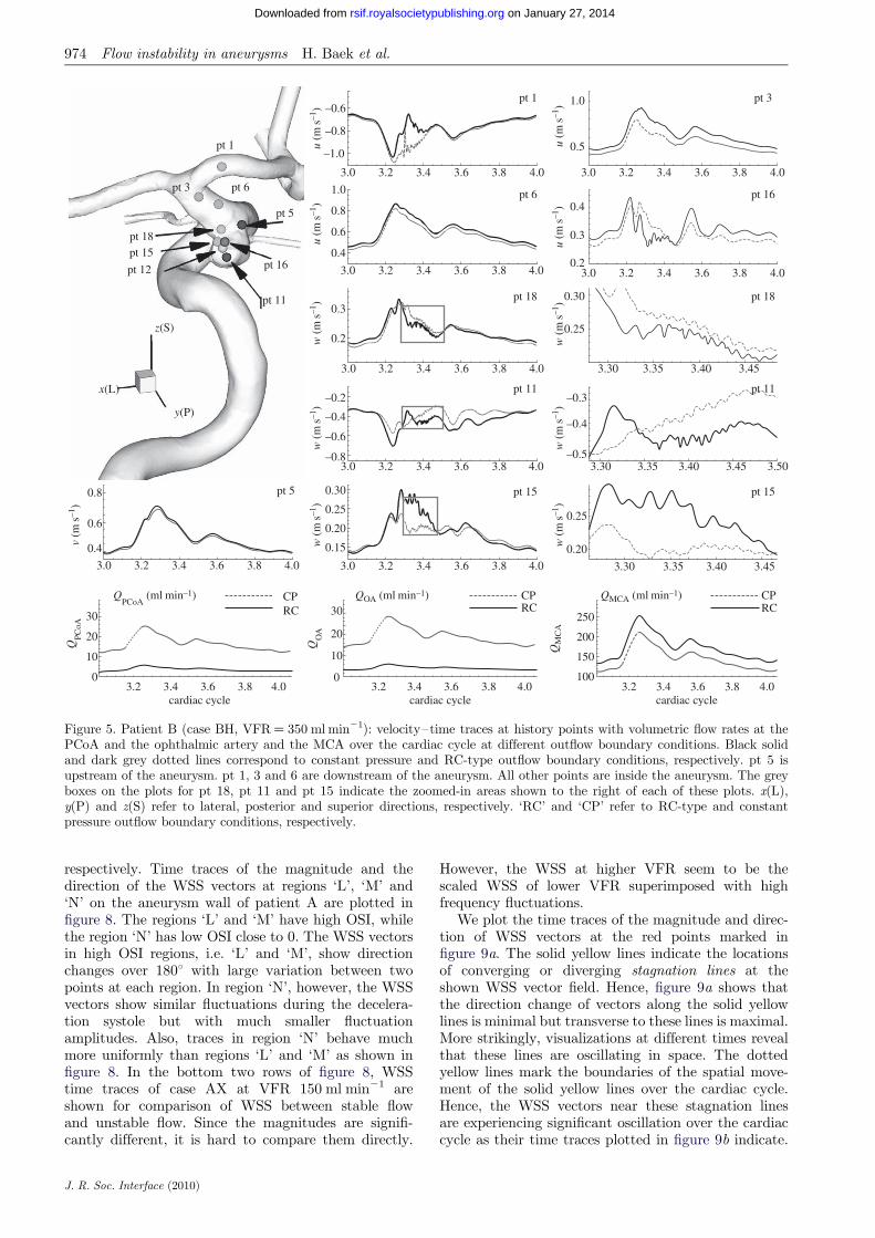
Inside the aneurysm of patient B, the stagnation areaexhibits a low WSS region surrounded by a band of highWSS as shown in figure 11b,c. The low WSS region hashigher pressure than the pressure in the adjacent wallsby 1 mm Hg. This pattern of WSS and pressure distri-bution agrees well with the experimental observations(Imbesi & Kerber 1999; Meng et al. 2007) in which itis pointed out that the high WSS region surroundsthe impingement point. This pattern of high/lowWSS is also noted from the upstream aneurysm ofpatient C as shown figure 10a. In this plot, the lowWSS region at the aneurysm fundus looks larger thanthat of patient B, but the surrounding high WSS isclearly observed. More dramatic is the spatial changein direction of WSS vectors around this spot; all WSSvectors point outward in radial directions over the

pow

er s

pect

ral d

ensi

typo

wer

spe

ctra

l den

sity

pow

er s

pect

ral d

ensi

ty

2(a)

(b)

(c)

f / fh = 16

f / fh = 12f / fh = 22

f / fh = 44f / fh = 28

f / fh = 10 f / fh = 24f / fh = 53

f / fh = 32f / fh = 50

0

–2

–4

2

2

–2

–4

–6

–8

0

f / fheart

0

–2

–4

0 50 100 150

Figure 7. Power spectral density of velocity–time traces at different history points for cases AH, BH, and CL. pt 10 of patient B islocated near the fundus of the aneurysm. pt 14 and pt 15 in patient A, and pt 1 in patient C, are shown either in figure 4 or 6. pt10 of patient B is similar location with pt 1 of patient C; both are near the fundus of the corresponding aneurysm. (c) shows thechanges in spectra at pt 14 of patient A as the average VFR increases from 150 to 250 ml min21. (a) Open square, pt 14,patient A; open triangle, pt 15 patient A. (b) Open diagonal triangle, pt 11 patient B; open circle, pt 1 patient C. (c) pt 14patient A: dashed line, VFR 150 ml min21; open triangle, VFR 200 ml min21; open diagonal triangle, VFR 250 ml min21.

976 Flow instability in aneurysms H. Baek et al.

on January 27, 2014rsif.royalsocietypublishing.orgDownloaded from

cardiac cycle. From this figure, it is clear that the flowimpinges near the fundus of the aneurysm forming thestagnation point and creating a high WSS areaaround the impingement (stagnation) area. It is alsointeresting that this critical location moves aroundduring the cardiac cycle; this is shown by the dots infigure 11b,c, which correspond to the lowest WSS spotat instants marked with dots of the corresponding col-ours. Therefore, a WSS vector at a fixed point nearthe stagnation area changes its direction ‘temporally’due to change in the impingement location over the car-diac cycle.

3.4. Flow structure inside the aneurysm

Next we examine temporal changes of global flow struc-tures inside the aneurysm such as the inflow/outflowregions and their changes along the depth are exam-ined. We present the flow structure inside theaneurysm of case CH because case CH shows the

J. R. Soc. Interface (2010)

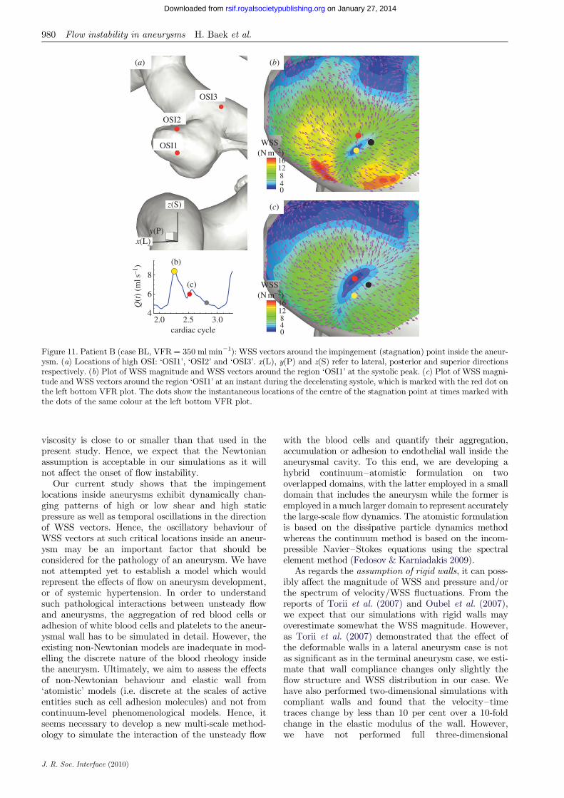
strongest instability among the three patients.Figure 12 shows the distribution of velocity componentnormal (a–d) or parallel (h– l ) to the plane on whichdata are extracted in case CH, VFR ¼ 200 ml min21.The planes and time instants for the velocity compu-tation are shown in figure 12f-1,2,g-1,2. The timeinterval between the time instants in figure 12f-2 isclose to the half period of the dominant velocity fluctu-ation. For comparison, black lines in figure 12h– l aredrawn as a reference, which is the border between thepositive and negative regions in figure 12i.

Comparison of normal velocity distribution amongfigure 12a–d shows that negative (into the aneurysm)and positive (out of the aneurysm) regions do notchange significantly over the cardiac cycle. Inside theaneurysm, the negative (inflow) region graduallymoves toward the distal part of the aneurysm alongthe depth, following the aneurysm wall due to the iner-tia until it impinges on the distal dome of the aneurysm.Although the flow is unstable as demonstrated in the

z(superior)

4

6 L

L

L

M

M

N

N

N

M

M (150 ml min–1)

L (150 ml min–1)N (150 ml min–1)

N (150 ml min–1)

2

0

0

10

100

100

1.0

0.5

0

0

510

30

4

2

0

–30

0

50

100

200

WSS

(N

m–2

)W

SS (

N m

–2)

WSS

(N

m–2

)an

gle

(°)

angl

e (°

)

WSS

(N

m–2

)W

SS (

N m

–2)

angl

e (°

)an

gle

(°)

2.2 2.4 2.6 2.8 3.0

2.2 2.4 2.6 2.8 3.0

2.2 2.4 2.6 2.8 3.0

2.2 2.4 2.6 2.8 3.0

30

–30

02

3

1

0

WSS

(N

m–2

)

2.2 2.4 2.6 2.8 3.0cardiac cyclecardiac cycle

(posterior)

(lateral)x y

Figure 8. Patient A (case AH, VFR ¼ 250 ml min21): left top shows the regions where WSS vectors are calculated; each regionhas two discrete points corresponding to the two curves in each plot. Time traces of magnitude and direction of WSS vectors ateach point are shown for each region ‘L’, ‘M’ and ‘N’. The angle of a WSS vector is calculated with reference to correspondingWSS vectors at the systolic peak. WSS time traces at VFR ¼ 150 ml min21 are shown for comparison purposes.

Flow instability in aneurysms H. Baek et al. 977

on January 27, 2014rsif.royalsocietypublishing.orgDownloaded from

time traces of velocity at history points in figure 6, flowstructures of positive and negative regions on planesover the cardiac cycle seem to change insignificantly.However, a closer look into the flow during the deceler-ating systole shows more changes as shown infigure 12h– l marked with black arrows, i.e. a patch ofnegative region appearing in the positive territory,and the countour lines crossing the black border line;these small scale changes are not significant enough tochange the global flow structure. While the velocityfluctuates inside the aneurysm, pressure also fluctuatesnear the wall with peak-to-peak magnitude of about

J. R. Soc. Interface (2010)

100–200 N m22 during the decelerating systole asshown in figure 13c. Pressure increases locally nearthe outer neck of the aneurysm wall, and a region ofpositive pressure difference Pn 2 Pm is clearly shownin figure 13a while the flow rate is decreasing.

4. DISCUSSION

Our study shows that flow instability may occur in cer-tain saccular aneurysms but not in all aneurysms.Specifically, the narrow-necked lateral aneurysm of

dire

ctio

n (°

)

200(a) (b)

z(S)

x(L)

L

M

WSS (N m–2)

605040302010

y(P)

20

100

10

–100

–200

0

0

L

L

dire

ctio

n (°

)

200

100

–100

–200

0

M

2005

4

3

2

0

10

MVFR

2.8 3.0 3.2 3.4 3.6cardiac cycle

2.8 3.0 3.2 3.4 3.6cardiac cycle

mag

nitu

de (

N m

–2)

mag

nitu

de (

N m

–2)

VFR

(m

l s–1

)

Figure 9. Patient C (case CH, VFR ¼ 200 ml min21): contour plot of WSS magnitude and WSS vectors, and time traces of themagnitude and direction change of WSS at two points, ‘L’ and ‘M’, on the wall. (a) Two points for computations of WSS magni-tude and angle are marked with red dots labelled ‘L’ and ‘M’. The solid yellow lines show the locations of the converging anddiverging lines at the current instant while the dotted yellow lines next to them indicate how far these stagnation lines moveover the cardiac cycle. (b) Time traces of WSS magnitude and angle changes at points ‘L’ and ‘M’. The left bottom plotshows the flow-rate profile and the red dot indicates the instant when the left snapshot was taken. x(L), y(P) and z(S) referto lateral, posterior and superior directions, respectively.

978 Flow instability in aneurysms H. Baek et al.

on January 27, 2014rsif.royalsocietypublishing.orgDownloaded from

patient B does not show velocity fluctuations seen inother patients until the VFR reaches 400 ml min21

which is beyond the physiologically correct VFR. Thisflow instability does not seem to be affected by flowrate changes in the bifurcations and small vessels asdocumented in our sensitivity study in appendix B.Moreover, this study has not considered terminal aneur-ysms. Based on the fact that wide-necked aneurysms inpatients A and C show much stronger velocity fluctu-ations from the VFR as low as 250 and 150 ml min21,we anticipate that flows in terminal aneurysms maybe more susceptible to instability.

Oscillations reported herein seem to be induced bya hydrodynamic instability that is described by theRayleigh inflection condition (Drazin & Reid 1981).Hydrodynamic instability and transition into turbu-lence in arterial pulsatile flow has been studiedextensively in the past (Nerem et al. 1972; Steiger &Reulen 1986; Einav & Sokolov 1993; Blackburn &Sherwin 2007). More recently, high-resolution simu-lations were performed for stenosed carotids by

J. R. Soc. Interface (2010)

Fischer et al. (2007), Lee et al. (2008) and Grinberget al. (2009). In all cases, turbulence or temporal fluctu-ations were observed in the decelerating systole or nearthe end of systole. The observed frequencies, however,are much higher than the frequencies observed in thecurrent work and intraoperative Doppler recordings ofSteiger & Reulen (1986). The reasons for the discre-pancy seem to be the different flow conditions such asthe much higher Reynolds number 1000–2000 of theflow in the aorta or the stenosed carotid. In the numeri-cal study of flow over periodic grooves in a channel byGhaddar et al. (1986), the frequency of the self-sustained oscillation corresponding to the least unstableTollmien–Schlichting mode was predicted from linearstability analysis. Our peak frequencies of patient C(around 24–58 Hz) seem to agree well with a frequencyrange (16–24 Hz) found in their study; this frequencyrange corresponds to frequencies in grooveswith non-dimensional separation distance L ¼ 5 andnon-dimensional groove length l ¼ 2.5 with differentdepth (non-dimensionalized with the half-channel

100z(S)

y(P)

x(L)

–100

0

L

dire

ctio

n (°

)m

agni

tude

(N

m–2

)di

rect

ion

(°)

mag

nitu

de (

N m

–2)

VFR

(m

l s–1

)

100

100

306

5

4

3

2

20

10

0

–100

033282318138

0

20

10

LM

WSS (N m–2)

L

M

M

cardiac cycle2.8 3.0 3.2 3.4 3.6

cardiac cycle2.8 3.0 3.2 3.4 3.6

VFR

(a) (b)

Figure 10. Patient C (case CH, VFR ¼ 200 ml min21): WSS magnitude and direction change at two points with contrastingcharacteristics on the upstream aneurysm at the systolic peak as marked with a red dot on the right bottom plot of VFR. (a)WSS vectors on the contour plot of WSS magnitude at the distal dome of the upstream aneurysm at the time indicated incycles. Two history points are marked with red dots labelled ‘L’ and ‘M’. (b) Corresponding time traces of the WSS magnitudeand direction change. The left bottom plot shows the flow-rate profile over the cardiac cycle. x(L), y(P) and z(S) refer to lateral,posterior and superior directions, respectively.

Flow instability in aneurysms H. Baek et al. 979

on January 27, 2014rsif.royalsocietypublishing.orgDownloaded from

width). The Reynolds numbers in our study based onthe flow rate and the kinematic viscosity are 877 and1271 on average and at the systolic peak, respectively.They are in good agreement with the critical Reynoldsnumber for the onset of instability which is close toRe ¼ 975 (Ghaddar et al. 1986).

Blood is a non-Newtonian fluid with shear-thinningand yield-stress. The effects of non-Newtonian propertyon the flow distribution in large arteries have beeninvestigated and some studies show dramatic effects(Gijsen et al. 1999a,b) while others report a smalleffect limited to a fraction of the cardiac cycle (Perktoldet al. 1991; Johnston et al. 2004). When the shear ratesare higher than 50 or 100 s21 (Long et al. 2004; Fischeret al. 2007), blood can be treated as a Newtonian fluidwith constant viscosity. In our simulations, we assumedthat the physiological flow rates in the ICA are in therange 200–250 ml min21, which gives an average vel-ocity in the range of 0.265–0.331 m s21. This is basedon the diameter of the ICA near the supraclinoidartery in our geometry, which is less than 4 mm, andthe characteristic shear rate 8Va/3r, 353–441 (s21),

J. R. Soc. Interface (2010)

where Va is the average velocity and r is the radius ofthe blood vessel. We confirmed that even inside theaneurysm, the shear rates are well above 100 s21 evenat the end of diastole. Our a posteriori analysis isshown in figure 14 with three non-Newtonian modelsand two different parameters per model, which are sum-marized in table 3. The characteristic shear rateffiffiffiffiffiffiffiffiffiffiffiffiffiffiffiffiffi

2 trðD2Þp

where Dij ¼ 1/2(@ui/@xj þ @uj/@xi), i, j ¼ 1,2, 3 (Macosko 1994) is above 100 s21 even at the endof diastole of a case with the smallest flow rate150 ml min21 except near the fundus of the downstreamaneurysm and near the centre of upstream ICA asshown in figure 14a,c. For example, the shear rates atthe black dots in figure 14b,d are 1352 and 1154.8 s21

for patient A and C, respectively. We also calculatethe ratio, m/mN, of apparent viscosity (m) using thethree non-Newtonian models, i.e. the Carreau,Carreau–Yasuda and Ballyk models, to the Newtonianviscosity (mN) used in our simulations as shown infigure 14b,c. Except for the centre of the aneurysm ofpatient A and of the parent vessels of patient C, theshear rates are well above 200 s21 and the apparent

(a) (b)

(c)

OSI3

1612840

8

1612840

(b)

(c)6

42.0 2.5

cardiac cycle3.0

OSI2

OSI1

z(S)

x(L)

Q(t

) (m

l s–1

)

y(P)

WSS (N m–2)

WSS (N m–2)

Figure 11. Patient B (case BL, VFR ¼ 350 ml min21): WSS vectors around the impingement (stagnation) point inside the aneur-ysm. (a) Locations of high OSI: ‘OSI1’, ‘OSI2’ and ‘OSI3’. x(L), y(P) and z(S) refer to lateral, posterior and superior directionsrespectively. (b) Plot of WSS magnitude and WSS vectors around the region ‘OSI1’ at the systolic peak. (c) Plot of WSS magni-tude and WSS vectors around the region ‘OSI1’ at an instant during the decelerating systole, which is marked with the red dot onthe left bottom VFR plot. The dots show the instantaneous locations of the centre of the stagnation point at times marked withthe dots of the same colour at the left bottom VFR plot.

980 Flow instability in aneurysms H. Baek et al.

on January 27, 2014rsif.royalsocietypublishing.orgDownloaded from

viscosity is close to or smaller than that used in thepresent study. Hence, we expect that the Newtonianassumption is acceptable in our simulations as it willnot affect the onset of flow instability.

Our current study shows that the impingementlocations inside aneurysms exhibit dynamically chan-ging patterns of high or low shear and high staticpressure as well as temporal oscillations in the directionof WSS vectors. Hence, the oscillatory behaviour ofWSS vectors at such critical locations inside an aneur-ysm may be an important factor that should beconsidered for the pathology of an aneurysm. We havenot attempted yet to establish a model which wouldrepresent the effects of flow on aneurysm development,or of systemic hypertension. In order to understandsuch pathological interactions between unsteady flowand aneurysms, the aggregation of red blood cells oradhesion of white blood cells and platelets to the aneur-ysmal wall has to be simulated in detail. However, theexisting non-Newtonian models are inadequate in mod-elling the discrete nature of the blood rheology insidethe aneurysm. Ultimately, we aim to assess the effectsof non-Newtonian behaviour and elastic wall from‘atomistic’ models (i.e. discrete at the scales of activeentities such as cell adhesion molecules) and not fromcontinuum-level phenomenological models. Hence, itseems necessary to develop a new multi-scale method-ology to simulate the interaction of the unsteady flow

J. R. Soc. Interface (2010)

with the blood cells and quantify their aggregation,accumulation or adhesion to endothelial wall inside theaneurysmal cavity. To this end, we are developing ahybrid continuum–atomistic formulation on twooverlapped domains, with the latter employed in a smalldomain that includes the aneurysm while the former isemployed in a much larger domain to represent accuratelythe large-scale flow dynamics. The atomistic formulationis based on the dissipative particle dynamics methodwhereas the continuum method is based on the incom-pressible Navier–Stokes equations using the spectralelement method (Fedosov & Karniadakis 2009).

As regards the assumption of rigid walls, it can poss-ibly affect the magnitude of WSS and pressure and/orthe spectrum of velocity/WSS fluctuations. From thereports of Torii et al. (2007) and Oubel et al. (2007),we expect that our simulations with rigid walls mayoverestimate somewhat the WSS magnitude. However,as Torii et al. (2007) demonstrated that the effect ofthe deformable walls in a lateral aneurysm case is notas significant as in the terminal aneurysm case, we esti-mate that wall compliance changes only slightly theflow structure and WSS distribution in our case. Wehave also performed two-dimensional simulations withcompliant walls and found that the velocity–timetraces change by less than 10 per cent over a 10-foldchange in the elastic modulus of the wall. However,we have not performed full three-dimensional

(a) (b) (c)

(d)

(h) (i) ( j) (k)

O

P

(a)

(b)

(c) (d)

D

O

SL

P

D

P

LS

O

PI

O D

I

I

P

P

(g-1)

(g-2) (f-2) ( l)

( f-1)

D

I 0.3

2.2 2.4 2.6cardiac cycle

cardiac cycle cardiac cycle

2.8 3.0

0.1–0.1–0.3

Vn (m s–1)

0.40

2.2 2.30 2.35 2.402.4 2.6 2.8 3.0

(h)(i)

(j)(k)

(l)

0.240.08

–0.08–0.24–0.40

Vc (m s–1)

Figure 12. Patient C (case CH, VFR ¼ 200 ml min21): distribution of normal or parallel velocity on a plane cutting through theaneurysm. In (a)–(d), positive velocity means flow out of the plane, showing inflow and outflow. In (h)–(l ), positive means flowalong the direction marked with the pink arrow in (i). This plane is taken at the neck and near the fundus of the aneurysm asshown in (g-1,2). (a–d) Normal velocity distribution at different phases of the cardiac cycle from the dicrotic peak, end of dia-stole, systolic peak and decelerating systole, respectively. (a,h) Letters ‘O’, ‘I’, ‘D’, and ‘P’ indicate the locations of the outer sideof the bend at the upstream aneurysm, of the inner side of the bend at the upstream aneurysm, of the distal portion of the aneur-ysm, and of the proximal portion of the aneurysm, respectively. ‘L’, ‘P’, and ‘S’ denote lateral, posterior and superior directions,respectively. ( f-1,2) and (g-1,2) show the time instants when the velocity fields are taken. (h– l ) Distribution of centreline velocityon the plane cutting through the aneurysm near the fundus of the aneurysm at five time instants marked with red dots at ( f-2).Black lines in (h)–(l ) mark the border line between positive and negative regions of (i). The black arrows in ( j) and (l ) mark thearea where changes from (i) and (k) are pronounced.

Flow instability in aneurysms H. Baek et al. 981

on January 27, 2014rsif.royalsocietypublishing.orgDownloaded from

simulations and the rigid wall assumption is alimitation of this study requiring further investigation.

5. CONCLUSIONS

Through a series of highly resolved CFD simulations,aneurysmal flow in wide-necked saccular intracranialaneurysms is shown to exhibit instabilities in the VFR

J. R. Soc. Interface (2010)

150–250 ml min21, which is lower than the meanVFR of 275 ml min21 with standard deviation+52 ml min21 (Ford et al. 2005). Flow in a narrow-necked lateral aneurysm becomes unstable as the VFRin the ICA reaches 400 ml min21. Specifically, weobserved that the pulsatile flow in aneurysms is subjectto a hydrodynamic instability during the deceleratingsystolic phase resulting in a high-frequency oscillation

300

250

L

P

S

200

1503.2 3.4 3.6 3.8

VFR

(m

l min

–1)

(a) (b)

2000

1800

1600

1400

12003.2 3.3

Pn

Pm

cardiac cycle3.4

P (

N m

–2)

ΔP (N m–2)

(c)

22013244

–44–132–220

Figure 13. Patient C (case CH, VFR ¼ 200 ml min21). (a) Distribution of pressure difference Pn 2 Pm at time instants markedwith circles on (c). (b) Volumetric flow rates over the cardiac cycle. (c) Time trace of pressure at a point indicated by an arrow in(a) during the time interval marked with a box in (b).

982 Flow instability in aneurysms H. Baek et al.

on January 27, 2014rsif.royalsocietypublishing.orgDownloaded from

over that period (Steiger& Reulen 1986). The flow returnsto its original pulsatile state near the end of diastole. Thefrequency of velocity fluctuations in our simulationsranges from 20 to 50 Hz, and is in good agreement withthe Doppler frequency recordings (Steiger & Reulen1986). Inside saccular aneurysms, the pattern aroundthe impingement areas shows relatively high staticpressure and low WSS region surrounded by a band ofhigher WSS. At such locations, the WSS vectors arespatially changing significantly in their direction. Owingto flow instability, the WSS vectors fluctuate in magni-tude and direction. In stagnation regions, the pressure/WSS patterns also fluctuate and move around spatially.The temporal change in these locations increases the tem-poral variation of WSS vectors. The oscillatory behaviourof WSS vectors, in combination with high/low WSS mag-nitude and locally elevated static pressure in stagnationareas, may play an important role in the formation andrupture of an aneurysm.

We would like to acknowledge support by the NSF OCI grants0845449, 0636336 and 0904288. Simulations were performedon the Cray XT3 (Bigben) at PSC, the Sun constellationlinux cluster (Ranger) at TACC and the Cray XT5(Kraken) at NICS.

APPENDIX A

A.1. Resolution studies (‘hp-refinement’ test)

We performed a systematic ‘hp-refinement’ test underthe same conditions used for our simulations. Thetime-dependent flow at the anatomically correct geo-metric model is tested at four different polynomialorders and four different meshes at fixed polynomialorder p ¼ 4. This study is intended to make sure thatthe oscillation is not due to numerical artefacts causedby under-resolution and to confirm that ourNEKTAR code can resolve high frequency oscillationcaused by the hydrodynamic instability. Hence, we

J. R. Soc. Interface (2010)

selected a case in which the velocity oscillates duringthe decelerating systole.

We used patient C’s two-aneurysm model. This geo-metric model was chosen because our study showedthat the flows in the two adjacent aneurysms are proneto become unstable. The type of element used for spacediscretization is tetrahedral. For p-refinement test,the tested polynomial orders are p ¼ 4, 6, 8, 10and the grid points used in the calculations are(p þ 3)(p þ 2)2 ¼ 252, 576, 1100, 1872 per element,respectively. Since the total number of elements is 89324, the total grid points per variable for polynomialorder p ¼ 10 is 167, 214, 528. The effective distancebetween grid points in this case is about 0.0091–0.0364 mm in the aneurysm, which is 110–440 timessmaller than the diameter of the inlet. For h-refinement,the number of elements are 81 162, 103 693 and 121 807with a polynomial order 4 and the reference was takenfrom the simulation with the largest number of elements121 807 and a higher order of polynomial ‘p ¼ 6’.

A.2. h-refinement

We checked convergence in the simulation using aspecific metric, the temporal average of spatial L2

error in WSS, against the results from a simulationwith the finest mesh as a reference using equation (A1). The frequency spectra of pointwise velocity arealso compared among the results from different meshes.

The formula for the WSS error calculation isdefined as

WSSe ¼1N

XN�1

i¼0

ÐjWSSi � gWSSij2 dS

� �1=2ÐdS

; ðA 1Þ

where the surface integration is done on the curved sur-face by numerical quadrature and the reference WSS( p ¼ 6, number of elements 121 000) is denoted bygWSS.

γ⋅200180160140120100806040200

1.051.031.010.990.970.95

μ /μN

1.051.031.010.990.970.95

μ /μN

γ⋅200180160140120100806040200

superior

posteriorlateral

superior

lateral

superiorsuperior

posteriorposterior lateral

lateral

10−2 1 102 10410−2

10−1

1

10

shear rate (s−1)

visc

osity

(P)

(a) (c)

(b)

(e)

(d )

posterior

Figure 14. Shear rate isocontours lower than 100 s21 at the end of diastole of patient A (a,b) and C (c,d). The ratio of apparentviscosity using Carraeu–Yasuda 1 (Cho & Kensey 1991) case to the Newtonian viscosity used in the simulations from the flowfields at the end of the diastole of patient A (a,b) and of patient C (c,d). Isosurfaces were extracted at the viscosity ratio 1.1.(e) Plot of apparent viscosity m versus shear rate (g). ‘Carreau 1’ and ‘Carreau 2’ refer to the Carreau model used in Lee &Steinman (2007) and Cho & Kensey (1991), respectively. ‘Carreau Yasuda 1’ and ‘Carreau Yasuda 2’ refer to the Carreau–Yasuda model used in Cho & Kensey (1991) and Gijsen et al. (1999b), respectively. ‘Ballyk 1’ and ‘Ballyk 2’ refer to theBallyk model used in Johnston et al. (2004) and Lee & Steinman (2007), respectively. Solid red line, Carreau 1; dot-dashedred line, Carreau 2; black solid line, Carreau Yasuda 1; dot-dashed black line, Carreau Yasuda 2; solid blue line, Ballyk 1;dot-dashed blue line, Ballyk 2.

Flow instability in aneurysms H. Baek et al. 983

on January 27, 2014rsif.royalsocietypublishing.orgDownloaded from

The frequency spectra are obtained from the timetraces at history points close to the points used inp-refinement test shown in figure 6 and a point in theupstream parent vessel during the entire third cardiaccycle. The WSS distribution on a patch shown in

J. R. Soc. Interface (2010)

figure 15a is calculated from the velocity field duringthe entire third cycle.

Convergence and spectra change: the L2 errors ofWSS from the h-refinement test show linear conver-gence over the number of elements or the size of

0.02z(S)

y(P)

x(L) 0.02

0.01

0.16

pow

er s

pect

ral d

ensi

ty

0.17 0.18

0.2

0.1

U (m

s−

1 )

0

0.10

V (m

s−

1 ) 0.15

3.4

3.3 3.4 3.5 4 5 6 7 8p

4 5 6 7 8pcardiac cycle

0.19 80 000 100 000 120 000no. of elementsh

10−1

10−1

10−2

10−2

10−3

10−4

10−3

10−2

10−3

10f / fh

20 30 40

1

(a)

(d)

(e)

( f )

(g) (h)

(b) (c)

Figure 15. (a) A patch where WSS errors are computed in reference to the highest polynomial order simulation (p ¼ 10) or thefinest mesh with higher order (p ¼ 6). Shading on the patch in the upstream aneurysm represents the x component of WSS vectorat the systolic peak. (b) Plot of WSS L2 error at the patch, which covers the upstream aneurysm walls, versus the largest edgelength. (c) Plot of WSS L2 error versus the number of elements. (d) The spectra at a history point inside the upstream aneurysmat different meshes. (e) Velocity–time traces at history point pt 1 inside the upstream aneurysm from four simulations with differ-ent polynomial order p ¼ 4, 6, 8, and 10. ( f ) Velocity–time traces at history point pt 10 inside the downstream aneurysm fromfour simulations with different polynomial order p ¼ 4, 6, 8, and 10. The differences between them, however, are not visuallydiscernible. (g) p-convergence of L2 error in WSS at the patch, which covers the upstream aneurysm walls, shown on the leftduring the time interval indicated with a grey box in figure 6. (h) L2 error of pointwise velocity at several history pointsshows spectral (exponential) convergence. (d) Square solid line, 80 000; triangle solid line, 103 000; inverted triangle solidline, 120 000; solid line, reference (h) Square solid line, pt 1; triangle solid line, pt 2; square dashed line, pt 4; diagonal triangledashed line, pt 6; diamond dashed line, pt 9; circle dashed line, pt 10.

Table 3. Non-Newtonian models and parameters used in the literature.

Carreau m ¼ m1 þ ðm0 � m1Þ½1þ ðl _gÞ2�ðn�1Þ=2

l ¼ 25 s; n ¼ 0:25 m0 ¼ 2:5P; m1 ¼ 0:035P Lee & Steinman (2007)l ¼ 3:313 s; n ¼ 0:3568 m0 ¼ 0:56P; m1 ¼ 0:0345P Cho & Kensey (1991)

Carreau–Yasuda model m ¼ m1 þ ðm0 � m1Þ 1þ ðl _gÞp½ �ðn�1Þ=p

l ¼ 1:902s; n ¼ 0:22 m0 ¼ 0:56P; m1 ¼ 0:0345P; p ¼ 1:25 Cho & Kensey (1991)l ¼ 0:11s; n ¼ 0:392 m0 ¼ 0:22P; m1 ¼ 0:022P; p ¼ 0:644 Gijsen et al. (1999b)

Ballyk model m ¼ lð _gÞðð _gÞÞnð _gÞ�1

lð _gÞ ¼ m1 þ Dm exp �ð1þ ð _g=aÞÞ expð�ðb= _gÞÞ½ �nð _gÞ ¼ n1 � Dn exp �ð1þ ð _g=cÞÞ expð�ðd= _gÞÞ½ �

n1 ¼ 1; Dn ¼ 0:45 m1 ¼ 0:0345P; Dm ¼ 0:25a ¼ 50; b ¼ 3; c ¼ 50; d ¼ 4 Johnston et al. (2004)

n1 ¼ 0:45; Dn ¼ 0:45 m1 ¼ 0:035P; Dm ¼ 0:25a ¼ 70:71; b ¼ 4:24; c ¼ 70:71; d ¼ 5:66 Lee & Steinman (2007)

984 Flow instability in aneurysms H. Baek et al.

J. R. Soc. Interface (2010)

on January 27, 2014rsif.royalsocietypublishing.orgDownloaded from

pt 24pt 17

pt 32

pt 19

pt 11

pt 22pt 2

pt 35

pt 3

pt 31

0.6

0.4

0.22.0 2.5

RC1pt 17RC2

CP

RC1RC2CP

RC1RC2CP

RC1RC2CP

RC1pt 19

pt 22 pt 24

pt 11pt 2

pt 31

pt 33 pt 35

pt 32

RC2CP

3.0 3.5

2.0 2.5 3.0 3.5

2.01.5 2.5 3.0 3.5

2.01.5S

L

P

2.5 3.0 3.5

2.01.5 2.5 3.0 3.5

2.0 2.5 3.0 3.5

2.0 2.5 3.0 3.5

2.0 2.5 3.0 3.5

2.0 2.5 3.0 3.5

2.0 2.5 3.0 3.52.0 2.5 3.0 3.5cardiac cycle

2.0

QPCoA (ml min–1) QMCA (ml min–1) QACA (ml min–1)

2.5 3.0 3.5cardiac cycle cardiac cycle

2.0 2.5 3.0 3.5

w (m

s–1

)

w (

m s

–1)0.6

0

–0.2

–0.4

0.4

0.2u (m

s–1

)

0.4

0.2w (m

s–1

) 0.20

0.15

0.10w (m

s–1

)

0.4

1006

4

2 50

100

150

50

v (m

s–1

)

0.3

0.2v (m

s–1

)

v (m

s–1

) 0.06

0.04

0.02

0

v (m

s–1

)

0.6

0.4

0.4

0.2

0.2

u (m

s–1

)

Figure 16. Patient C (case CL, VFR ¼ 150 ml min21): comparison of velocity–time traces at history points upstream and down-stream of the aneurysms among different outflow boundary conditions. Velocity–time traces at the upstream history points showthat the upstream flow is stable over the cardiac cycle and instability occurs in the aneurysms. ‘RC1’, ‘RC2’, and ‘CP’ refer toRC-type 1, RC-type 2 and constant pressure outflow boundary conditions, respectively.

Flow instability in aneurysms H. Baek et al. 985

on January 27, 2014rsif.royalsocietypublishing.orgDownloaded from

element edge as shown in figure 15b,c. Spectra fromdifferent meshes show similar peaks and the changesare insignificant among them as shown in figure 15d.

A.3. p-refinement

We checked convergence in the simulation using twometrics: the L2 error in time of pointwise velocity andtemporal average of spatial L2 error in WSS. Theerrors are compared against the results from a simu-lation with the highest order polynomial, i.e. p ¼ 10,as a reference.

Simulations for error computations start from thesystolic peak and continue until the dicrotic peak forthe aforementioned reasons. This time interval forerror computation is about one-sixth of the cardiaccycle as indicated by the grey box in figure 6.

The history points and the time interval duringwhich temporal averages were taken are shown infigure 6. A patch on which WSS errors are computedis shown in figure 15a. The formula for WSS error

J. R. Soc. Interface (2010)

calculation is equation (A 1), where the surface inte-gration is done on the curved surface by numericalquadrature and the reference WSS (p ¼ 10) is denotedby gWSS. The velocity error at each history point istaken as

Ve ¼PN�1

i¼0 jVi � eVij2PN�1i¼0 jeVij2

!1=2

; ðA 2Þ

where the reference velocity (p ¼ 10) is denoted by eV .We performed a simulation with polynomial order

p ¼ 6 up to four cardiac cycles. During the last cycle,the check points files were saved every time unit withtime step Dt ¼ 0.00025. Using the check point file atthe systolic peak of the fourth cycle, three more simu-lations with different polynomial orders, i.e. p ¼ 4, 8,and 10, were performed with the same time step,which satisfies the CFL condition for all polynomialorders.

986 Flow instability in aneurysms H. Baek et al.

on January 27, 2014rsif.royalsocietypublishing.orgDownloaded from

Convergence: time traces of velocity at two historypoints are plotted in figure 15f showing no discernibledifference. The L2 errors of WSS and velocity fromthe p-refinement test show exponential convergenceover the order of polynomial as shown in figure 15g,h,respectively. Average WSS over the patch is about10 N m22 and the error changes from 0.2956 N m22

( p ¼ 6) to 0.0591 N m22 ( p ¼ 8). Hence, they areabout 3 and 0.6 per cent of the average WSS. Forvelocity, errors are even smaller: 0.1 per cent ( p ¼ 6)and 0.01 per cent ( p ¼ 8). WSS has one orderlower accuracy because WSS is calculated throughdifferentiation of field variables.

APPENDIX B. EFFECT OF OUTFLOWCONDITIONS

Figure 5 shows quantitative changes in the flow whenflow rates at the outlets change by a factor of 5 insmall arteries and by 20 per cent in large outlets ofpatient B. Specifically, using RC boundary conditions,the flow rates at the PCoA and the ophthalmic arteryare reduced by factor of 5, and the increase in MCAflow rate compensates the flow reduction in the smallarteries. The velocity–time traces at the upstreamand downstream history points are plotted and com-pared between constant pressure (CP) and RC-type(RC) outflow boundary condition. Velocities at morepoints are examined as well as the points in figure 5.The zoom-in plots of time traces at pt 11, 15, and 18show that the frequencies of small fluctuations do notchange although the magnitudes of fluctuation changesomewhat at some history points. The peak at pt 1seems to disappear due to the flow rate increase in theMCA. However, the flow rate changes seem not toaffect the flow instability.

Figure 16 shows flow rate changes in the MCA/ACA.In this case, we apply two different RC boundary con-ditions, one of which (RC1) makes the flow rates closeto those corresponding to the constant pressure con-dition. By imposing the other RC outflow boundary(RC2) condition, we increase the VFR at the MCAand reduce the flow at the ACA by 30 per cent.Upstream history points do not show any high fre-quency oscillations seen in velocity–time traces athistory points inside the aneurysms. Velocity–timetraces at history points inside the aneurysms andupstream of aneurysms are almost the same amongthe different boundary conditions. Those downstreamof the aneurysms show different magnitudes but similarfluctuations. Hence, we conclude that outlet flow ratesdo not seem to affect aneurysmal flow instability.

REFERENCES

Baek, H., Jayaraman, M. & Karniadakis, G. 2007 Distributionof WSS on the internal carotid artery with an aneurysm: aCFD sensitivity study. In Proc. ASME Int. MechanicalEngineering Congress and Exposition 2007, vol. 2,pp. 29–36. New York, NY: ASME.

J. R. Soc. Interface (2010)

Batchelor, G. K. 1956 On steady laminar flow with closedstreamlines at large Reynolds number. J. Fluid Mech. 1,177–190. (doi:10.1017/S0022112056000123)

Blackburn, H. M. & Sherwin, S. J. 2007 Instability modes andtransition of pulsatile stenotic flow: pulse-period depen-dence. J. Fluid Mech. 573, 57–88. (doi:10.1017/S0022112006003740)

Boussel, L. et al. 2008 Aneurysm growth occurs at regionof low wall shear stress: patient-specific correlation ofhemodynamics and growth in a longitudinal study.Stroke 39, 2997–3002. (doi:10.1161/STROKEAHA.108.521617)

Castro, M. A., Putman, C. M. & Cebral, J. R. 2006Computational fluid dynamics modeling of intracranialaneurysms: effect of parent artery segmentation on intra-aneurysmal hemodynamics. Am. J. Neuroradiol. 27,1703–1709.

Cebral, J. R., Castro, M. A., Appanaboyina, S., Putman,C. M., Millan, D. & Frangi, A. F. 2005a Efficient pipelinefor image-based patient-specific analysis of cerebral aneur-ysm hemodynamics technique and sensitivity. IEEETrans. Med. Imaging 24, 457–467. (doi:10.1109/TMI.2005.844159)

Cebral, J. R., Castro, M. A., Burgess, J. E., Pergolizzi, R. S.,Sheridan, M. J. & Putman, C. M. 2005b Characterizationof cerebral aneurysms for assessing risk of rupture byusing patient-specific computational hemodynamicsmodels. Am. J. Neuroradiol. 26, 2550–2559.

Cebral, J. R., Radaelli, A., Frangi, A. & Putman, C. M. 2007Hemodynamics before and after bleb formation in cerebralaneurysms. Proc. SPIE 6511, 65112C. (doi:10.1117/12.709240)

Cebral, J. R., Hendrickson, S. & Putman, C. M. 2009 Hemo-dynamics in a lethal basilar artery aneurism just before itsrupture. Am. J. Neuroradiol. 30, 95–98. (doi:10.3174/ajnr.A1312)

Chatziprodromou, I., Tricoli, A., Poulikakos, D. & Ventikos, Y.2007 Haemodynamics and wall remodelling of a growingcerebral aneurysm: a computational model. J. Biomech.40, 412–426. (doi:10.1016/j.jbiomech.2005.12.009)

Cho, Y. I. & Kensey, K. R. 1991 Effect of the non-Newtonianviscosity of blood on hemodynamics of diseasedarterial flows: part 1, steady flows. Biorheology 28,241–262.

Deane, C. R. & Markus, H. S. 1997 Colour velocity flowmeasurement: in vitro validation and application tohuman carotid arteries. Ultrasound Med. Biol. 23,447–452. (doi:10.1016/S0301-5629(96)00224-4)

Drazin, P. G. & Reid, W. H. 1981 Hydrodynamic stability,pp. 131–133. Cambridge, UK: Cambridge UniversityPress.

Einav, S. & Sokolov, M. 1993 An experimental study ofpulsatile pipe flow in the transition range. J. Biomech.Eng. 115, 404–411. (doi:10.1115/1.2895504)

Fedosov, D. A. & Karniadakis, G. E. 2009 Triple-decker:interfacing atomistic-mesoscopic-continuum flow regimes.J. Comput. Phys. 228, 1157–1171. (doi:10.1016/j.jcp.2008.10.024)

Ferguson, G. G. 1970 Turbulence in human intracranialsaccular aneurysms. J. Neurosurg. 33, 485–497. (doi:10.3171/jns.1970.33.5.0485)

Fischer, P. F., Loth, F., Lee, S. E., Lee, S.-W., Smith, D. S. &Bassiouny, H. S. 2007 Simulation of high-Reynolds numbervascular flows. Comput. Meth. Appl. Mech. Eng. 196,3049–3060. (doi:10.1016/j.cma.2006.10.015)

Ford, M. D., Alperin, N., Lee, S. H., Holdsworth, D. W. &Steinman, D. A. 2005 Characterization of volumetric flowrate waveforms in the normal internal carotid and

Flow instability in aneurysms H. Baek et al. 987

on January 27, 2014rsif.royalsocietypublishing.orgDownloaded from

vertebral arteries. Physiol. Meas. 26, 477–488. (doi:10.1088/0967-3334/26/4/013)

Ghaddar, N. K., Korczak, K. Z., Mikic, B. B. & Patera, A. T.1986 Numerical investigation of incompressible flow ingrooved channels. Part 1. Stability and self-sustainedoscillations. J. Fluid Mech. 163, 99–127. (doi:10.1017/S0022112086002227)

Gijsen, F. J. H., Allanic, E., van de Vosse, F. N. & Janssen, J.D. 1999a The influence of the non-Newtonian properties ofblood on the flow in large arteries: unsteady flow in a 908curved tube. J. Biomech. 32, 705–713. (doi:10.1016/S0021-9290(99)00014-7)

Gijsen, F. J. H., van de Vosse, F. N. & Janssen, J. D. 1999bThe influence of the non-Newtonian properties of bloodon the flow in large arteries: steady flow in a carotid bifur-cation model. J. Biomech. 32, 601–608. (doi:10.1016/S0021-9290(99)00015-9)

Grinberg, L. & Karniadakis, G. E. 2008 Outflow boundaryconditions for arterial networks with multiple outlets.Ann. Biomed. Eng. 36, 1496–1514. (doi:10.1007/s10439-008-9527-7)

Grinberg, L., Yakhot, A. & Karniadakis, G. E. 2009 Analyz-ing transient turbulence in a stenosed carotid artery byproper orthogonal decomposition. Ann. Biomed. Eng. 37,2200–2217. (doi:10.1007/s10439-009-9769-z)

Imbesi, S. G. & Kerber, C. W. 1999 Analysis of slipstream flowin two ruptured intracranial cerebral aneurysms.Am. J. Neuroradiol. 20, 1703–1705.

Johnston, B. M., Johnston, P. R., Corney, S. & Kilpatrick, D.2004 Non-Newtonian blood flow in human right coronaryarteries: steady state simulations. J. Biomech. 37,709–720. (doi:10.1016/j.jbiomech.2003.09.016)

Jou, L.-D., Lee, D., Morsi, H. & Mawad, M. 2008 Wall shearstress on ruptured and unruptured intracranial aneurysmsat the internal carotid artery. Am. J. Neuroradiol. 29,1761–1767. (doi:10.3174/ajnr.A1180)

Karniadakis, G. E. & Sherwin, S. J. 2005 Spectral/hpelement methods for CFD. Oxford, UK: Oxford UniversityPress.

Lee, S.-W. & Steinman, D. A. 2007 On the relative importanceof rheology for image-based CFD models of the carotidbifurcation. J. Biomech. Eng. 129, 273–278. (doi:10.1115/1.2540836)

Lee, S. E., Lee, S.-W., Fischer, P. F., Bassiouny, H. S. & Loth,F. 2008 Direct numerical simulation of transitional flow ina stenosed carotid bifurcation. J. Biomech. 41, 2551–2561.(doi:10.1016/j.jbiomech.2008.03.038)

Lighthill, M. J. 1975 Mathematical biofluiddynamics,pp. 206–208. Philadelphia, PA: SIAM.

Long, D. S., Smith, M. L., Pries, A. R., Ley, K. & Damiano,E. R. 2004 Microviscometry reveals reduced blood viscosityand altered shear rate and shear stress profiles in microves-sels after hemodilution. Proc. Natl Acad. Sci. USA 101,10 060–10 065. (doi:10.1073/pnas.0402937101)

Macosko, C. W. 1994 Rheology: principles, measurements andapplications. New York, NY: Wiley.

Magnenat-Thalmann, N. & Thalmann, D. 2005 Handbook ofvirtual humans. New York, NY: Wiley.

Malek, A., Alper, S. & Izumo, S. 1999 Hemodynamic shearstress and its role in atherosclerosis. J. Am. Med. Assoc.282, 2035–2041. (doi:10.1001/jama.282.21.2035)

Marks, M. P., Pelc, N. J., Ross, M. R. & Enzmann, D. R. 1992Determination of cerebral blood flow with a phase-contrastcine MR imaging technique: evaluation of normal subjectsand patients with arteriovenous malformations. Radiology182, 467–476.

Marshall, I., Papathanasopoulou, P. & Wartolowska, K. 2004Carotid flow rates and flow division at the bifurcation in

J. R. Soc. Interface (2010)

healthy volunteers. Physiol. Meas. 25, 691–697. (doi:10.1088/0967-3334/25/3/009)

Meng, H., Wang, Z., Hoi, Y., Gao, L., Metaxa, E., Swartz,D. D. & Kolega, J. 2007 Complex hemodynamics atthe apex of an arterial bifurcation induces vascularremodeling resembling cerebral aneurysm initiation.Stroke 38, 1924–1931. (doi:10.1161/STROKEAHA.106.481234)

Moore, J. E., Xu, C., Glagov, S., Zarins, C. K. & Ku, D. N.1994 Fluid wall shear stress measurements in a model ofthe human abdominal aorta: oscillatory behavior andrelationship to atherosclerosis. Atherosclerosis 110, 225–240. (doi:10.1016/0021-9150(94)90207-0)

Moyale, K. R., Antiga, L. & Steinman, D. A. 2006 Inlet con-ditions for image-based CFD models of the carotidbifurcation: is it reasonable to assume fully developedflow? J. Biomech. Eng. 128, 371–379. (doi:10.1115/1.2187035)

Murayama, Y., Nien, Y. L., Duckwiler, G., Gobin, Y. P.,Jahan, R., Frazee, J., Martin, N. & Vinuela, F. 2003Guglielmi detachable coil embolization of cerebral aneur-ysms: 11 years’ experience. J. Neurosurg. 98, 959–966.(doi:10.3171/jns.2003.98.5.0959)

Nerem, R. M., Seed, W. A. & Wood, N. B. 1972 An exper-imental study of the velocity distribution and transitionto turbulence in the aorta. J. Fluid Mech. 52, 137–160.(doi:10.1017/S0022112072003003)

Oshima, M., Sakai, H. & Torii, R. 2005 Modeling of inflowboundary conditions for image-based simulation ofcerebrovascular flow. Int. J. Numer. Meth. Fluids 47,603–617. (doi:10.1002/fld.834)

Oubel, E., Craene, M. D., Putman, C. M., Cebral, J. R. &Frangi, A. F. 2007 Analysis of intracranial aneurysm wallmotion and its effect on hemodynamics patterns. Proc.SPIE Med. Imaging 6511, 651 12A. (doi:10.1117/12.708937)

Perktold, K., Resch, M. & Florian, H. 1991 Pulsatile non-Newtonian flow characteristics in a three-dimensionalhuman carotid bifurcation model. J. Biomech. Eng. 113,464–475. (doi:10.1115/1.2895428)

Rockwell, D. & Naudascher, E. 1979 Self-sustained oscil-lations of impinging free shear layers. Annu. Rev. FluidMech. 11, 67–94. (doi:10.1146/annurev.fl.11.010179.000435)

Sekhar, L. N. & Wasserman, J. F. 1984 Noninvasive detectionof intracranial vascular lesions using an electronic stetho-scope. J. Neurosurg. 60, 553–559. (doi:10.3171/jns.1984.60.3.0553)

Sekhar, L. N., Sun, M., Bonaddio, D. & Scalbassi, R. J. 1991Acoustic recordings from experimental saccular aneurysmsin dogs. Stroke 21, 1215–1221.

Sforza, D. M., Putman, C. M. & Cebral, J. R. 2009Hemodynamics of cerebral aneurysms. Annu. Rev. FluidMech. 41, 91–107. (doi:10.1146/annurev.fluid.40.111406.102126)

Sherwin, S. J., Shah, O., Doorly, D. J., Papaharilaou, Y.,Watkins, N., Caro, C. G. & Dumoulin, C. L. 2000 Theinfluence of out-of-plane geometry on the flow within adistal end-to-side anastomosis. J. Biomech. Eng. 122,86–95. (doi:10.1115/1.429630)

Simkins, T. E. & Stehbens, W. E. 1974 Vibrations recordedfrom the adventitial surface of experimental aneurysmsand arteriovenous fistulas. Vasc. Surg. 8, 153–165.

Steiger, H. J. & Reulen, H.-J. 1986 Low frequency flowfluctuations in saccular aneurysms. Acta Neurochir. 83,131–137. (doi:10.1007/BF01402392)

Steiger, H. J., Poll, A., Liepsch, D. & Reulen, H.-J. 1987Basic flow structure in saccular aneurysms: a flow

988 Flow instability in aneurysms H. Baek et al.

on January 27, 2014rsif.royalsocietypublishing.orgDownloaded from

visualization study. Heart Vessels 3, 55–65. (doi:10.1007/BF02058520)

Straatman, A. G., Khayat, R. E., Haj-Qasem, E. & Steinman,D. A. 2002 On the hydrodynamic stability of pulsatile flowin a plane channel. Phys. Fluids 14, 1938–1944. (doi:10.1063/1.1476673)

Szymanski, M. P., Metaxa, E., Meng, H. & Kolega, J. 2008Endothelial cell layer subjected to impinging flow mimick-ing the apex of an arterial bifurcation. Ann. Biomed. Eng.10, 1681–1689. (doi:10.1007/s10439-008-9540-x)

Tateshima, S., Vinuela, F., Vilablanca, J. P., Murayama, Y.,Morino, T., Nomura, K. & Tanishita, K. 2003 Three-

J. R. Soc. Interface (2010)

dimensional blood flow analysis in a wide-necked internalcarotid artery-ophthalmic artery aneurysm. J. Neurosurg.99, 526–533. (doi:10.3171/jns.2003.99.3.0526)

Torii, R., Oshima, M., Kobayashi, T., Takagi, K. & Tezduyar,T. E. 2006 Fluid–structure interaction modeling of aneu-rysmal conditions with high and normal blood pressures.Comput. Mech. 38, 482–490. (doi:10.1007/s00466-006-0065-6)

Torii, R., Oshima, M., Kobayahsi, T., Takagi, K. & Tezduyar,T. E. 2007 Influence of wall elasticity in patient-specifichemodynamic simulations. Comput. Fluids 36, 160–168.(doi:10.1016/j.compfluid.2005.07.014)