Flow Measurement and Instrumentation 76 (2020) 101811

Available online 3 September 20200955-5986/Published by Elsevier Ltd.

Modeling temperature effects on a Coriolis mass flowmeter

Fabio Ouverney Costa a, Jodie G. Pope b,*, Keith A. Gillis b

a Instituto Nacional de Metrologia/Directory of Scientific and Industrial Metrology/Fluid Dynamics Metrology Division, Duque de Caxias, RJ, Brazil b Fluid Metrology Group, National Institute of Standards and Technology, Gaithersburg, MD, USA

A R T I C L E I N F O

Keywords: Coriolis meter Temperature-effects Physical model Flowmeter Cryogenic

A B S T R A C T

Coriolis mass flowmeters are used for many applications, including as transfer standards for proficiency testing and liquified natural gas (LNG) custody transfer. We developed a model to explain the temperature dependence of a Coriolis meter down to cryogenic temperatures. As a first step, we tested our model over the narrow tem-perature range of 285 K to 318 K in this work. The temperature dependence predicted by the model agrees with experimental data within ± 0.08 %; the model uncertainty is 0.16 % (95 % confidence level) over the tem-perature range of this work.

Here, basic concepts of Coriolis flowmeters will be presented, and correction coefficients will be proposed that are valid down to 5 K based on literature values of material properties.

1. Introduction

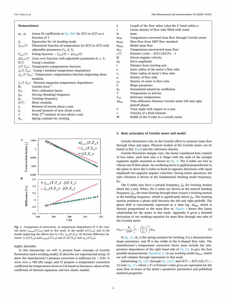
We developed a model to explain the temperature dependence of mass flow measurements using Coriolis meters which we expect to work down to cryogenic temperatures. The goal of this work is to: 1) quantify the errors due to inaccurate temperature corrections and thereby enable more accurate use of the meter as a transfer mass flow standard, and 2) allow Coriolis meters to be calibrated in water and used for liquified natural gas (LNG) transfer with little loss of accuracy. We tested our model over the temperature range of 285 K to 318 K in this work. The temperature dependence predicted by the model agrees with experi-mental data within ± 0.08 %; the model’s uncertainty is 0.16 % (k = 2, corresponding to a 95 % confidence level). Fig. 1 shows this agreement and will be discussed in detail in Section 5.

Coriolis mass flowmeters are known to be stable, have low uncer-tainty (± 0.1 %), and are insensitive to fluid properties. This meter type is used for many applications, including as transfer standards for profi-ciency testing and LNG custody transfer. The meter’s flow tubes are constructed of materials that can significantly affect the meter’s accu-racy as the pressure and temperature of the fluid inside them changes. Stainless steels are commonly used for flow tube construction due to their corrosion resistance. The meter used in this study was constructed from 316 stainless steel. Below 100 K, the temperature dependences of Young’s modulus E(T) and the shear modulus G(T) for 316 stainless steel are nonlinear, as shown in Fig. 2 [1]. Therefore, we developed a model to explain and correct how these elastic constants effect a Coriolis

meter’s measurements. We disabled the manufacturer’s temperature compensation in a

single, dual-tube, 5 cm diameter Coriolis meter to test for the accuracy of our model over the temperature range of 285 K to 318 K. We verified that the manufacturer’s pressure correction was accurate; therefore, the remaining deviations were due to temperature effects on the meter.

The use of a low uncertainty, reproducible flowmeter (or transfer standard) for lab-to-lab proficiency testing is highly desirable. The un-certainty, including the reproducibility should be “much less” than the uncertainty of the flow laboratory’s being testing [2]. Coriolis meters have been thought to be able to provide the desired traits of an acceptable transfer standard. However, unexplained lab-to-lab varia-tions have been observed in unpublished work that have led us to investigate more closely how these meters work. Given that flow labs typically do not have matching temperature and pressure conditions, the effects of these parameters on meter performance was investigated.

Due to a lack of calibration facilities that operate at cryogenic tem-peratures, it is important to quantify the effects of temperature on the meter’s calibration down to LNG temperatures (111 K). We predict the effects of temperature down to 5 K. As a first step, in this work we verified this prediction over the limited temperature range that was accessible to our standard (285 K to 318 K). In a future publication, we will refine and test our model down to at LN2 temperatures (77 K) using NIST’s cryogenic flow measurement facility [3,4], which ceased oper-ation in December of 2019. Cryogenic facilities are expensive to build and maintain. Calibration of a Coriolis meter at a water flow facility with little or no loss of accuracy at cryogenic temperatures is, therefore,

* Corresponding author. E-mail address: jodie.pope@nist.gov (J.G. Pope).

Contents lists available at ScienceDirect

Flow Measurement and Instrumentation

journal homepage: http://www.elsevier.com/locate/flowmeasinst

https://doi.org/10.1016/j.flowmeasinst.2020.101811 Received 2 April 2020; Received in revised form 7 July 2020; Accepted 17 August 2020

Flow Measurement and Instrumentation 76 (2020) 101811

2

highly desirable. In this manuscript, we will 1) present basic concepts of Coriolis

flowmeters and a working model; 2) describe our experimental setup; 3) show the manufacturer’s pressure correction is sufficient for < 0.01 % error over a 700 kPa range; and 4) propose a temperature correction coefficient for temperatures down to 5 K based on literature values of the coefficient of thermal expansion and two elastic moduli.

2. Basic principles of Coriolis meter and model

Coriolis flowmeters rely on the Coriolis effect to measure mass flow through tubes and pipes. Physical models of the Coriolis meter can be found in Ref. [5,6] and the references therein.

Coriolis flowmeter designs vary; the meter considered here consists of two tubes, each bent into a U shape with the ends of the straight segments rigidly mounted as shown in Fig. 3. The U-tubes are free to vibrate out of their plane. An oscillating force is applied perpendicular to the plane to drive the U-tubes to bend in opposite directions with equal amplitude but opposite angular velocities. During meter operation, the tube vibration is driven at the fundamental bending mode frequency, fnb.

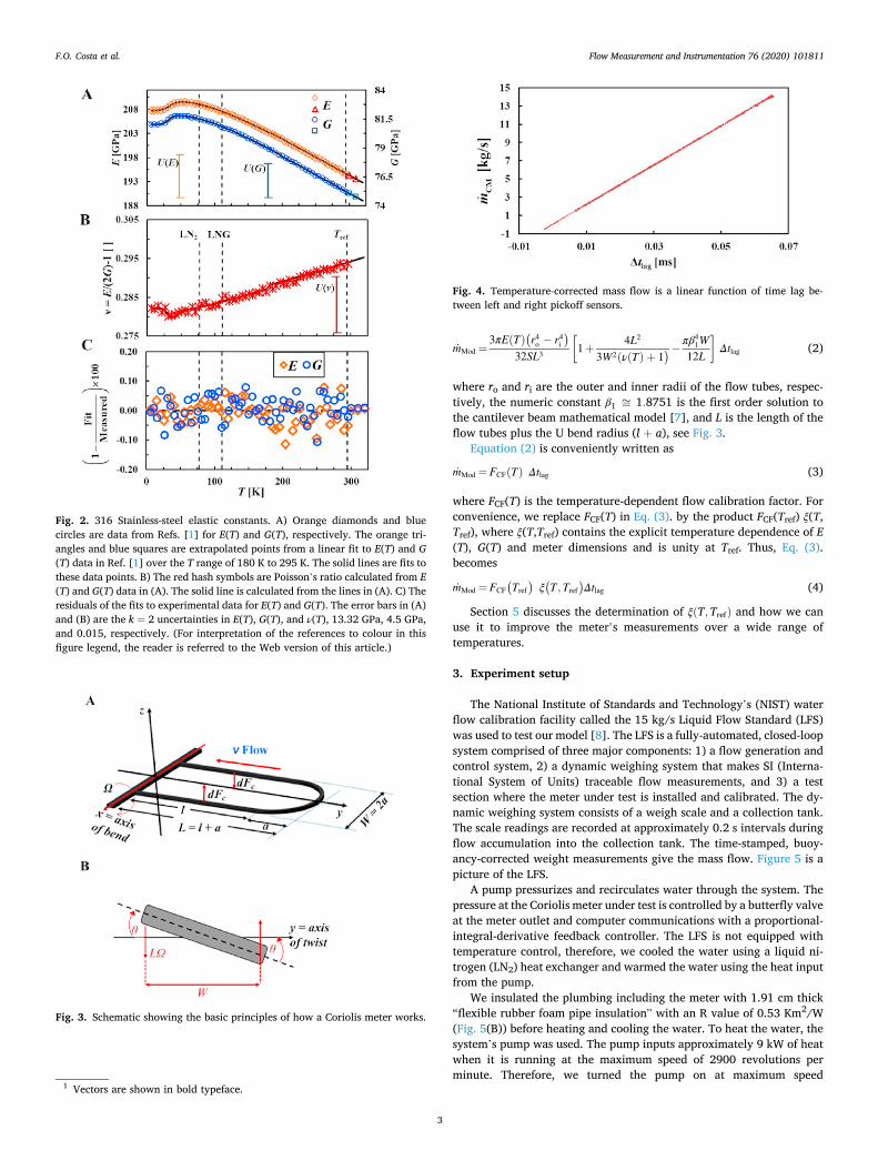
The U-tubes also have a natural frequency, fnt for twisting motion about the y-axis. When, the U-tubes are driven at the natural bending frequency, fnb, the mass flowing through them creates a twisting motion at the bending frequency, which is significantly below fnt. The twisting motion produces a phase shift between the left and right pickoffs. The phase shift is conveniently expressed as a time lag, Δtlag, which is directly proportional to the mass flow m. Figure 4 shows this linear relationship for the meter in this study. Appendix A gives a detailed derivation of our working equation for mass flow through one tube of the Coriolis meter

mMod =Ku

2SW2

[

1 −(

fnb

fnt

)2]

Δtlag (1)

In Eq. (1), Ku is the spring constant for twisting, S is a dimensionless shape parameter, and W is the width of the U-shaped flow tube. The manufacturer’s temperature correction factor must include the tem-perature dependence of the right hand side of Eq. (1). to give the best possible measurements. Equation (1) is our working model mMod, which we will validate through experiment in this work.

Substituting Eq. (A3) through Eq. (A11) and G(T) = E(T)/[2(ν(T) +1)] into Eq. (1), where ν(T) is Poisson’s ratio gives an expression for the mass flow in terms of the meter’s geometric parameters and published material properties

Nomenclature

a0, a1 Linear fit coefficients in Eq. (B4) for E(T) or G(T) as a function of T

β1 Eigenvalue for 1st bending mode CE,G(T) Theoretical function of temperature for E(T) or G(T) with

adjustable parameters C0, d, T0

C′

E,G(T) Fitting function = CE,G(T) + ΔCE,G(T) ΔCE,G(T) Cross over function with adjustable parameters b, c, Ts

E(T) Young’s modulus ξ(T,Tref) Temperature compensation function ξE(T,Tref) Young’s modulus temperature dependence ξE,α(T,Tref) Temperature compensation function neglecting shear

modulus ξα(T,Tref) Thermal expansion temperature dependence FC Coriolis force11

FCF Flow calibration factor fnb Driving (bending) frequency fnt Twisting frequency G(T) Shear modulus Iy Moment of inertia about y-axis Ix Second moment of area about y-axis J Polar 2nd moment of area about z-axis Ku Spring constant for twisting

L Length of the flow tubes l plus the U bend radius a λ Linear density of flow tube filled with water m mass mCM Temperature-corrected mass flow through Coriolis meter mNIST Mass flow from NIST flow standard mMod Model mass flow mUC Temperature-uncorrected mass flow ν(T) Poisson’s ratio = E(T)/(2G(T)) – 1 Ω Driven angular velocity Ω0 Drive amplitude r Distance from twisting axis ri Inner radius of the meter’s flow tube ro Outer radius of meter’s flow tube ρt Density of flow tube ρw Density of water in flow tube S Shape parameter SN Normalized sensitivity coefficient T Temperature in kelvins Tref Reference temperature Δtlag Time difference between Coriolis meter left and right

pickoff phases θ Twist angle with respect to y-axis v Velocity of a fluid element W Width of the U-tube in a coriolis meter

Fig. 1. Comparison of corrections. A) temperature dependence of 1) the Cori-olis meter ξmeter(T,Tref) used in this work, 2) the model ξ(T,Tref), and 3) the model neglecting the effects due to ν(T), ξE,α(T,Tref). B) Percent difference be-tween 1) ξ(T,Tref) and ξmeter(T,Tref) and 2) ξ(T,Tref) and ξE,α(T,Tref).

F.O. Costa et al.

Flow Measurement and Instrumentation 76 (2020) 101811

3

mMod =3πE(T)

(r4

o − r4i

)

32SL3

[

1+4L2

3W2(ν(T) + 1) −

πβ41W

12L

]

Δtlag (2)

where ro and ri are the outer and inner radii of the flow tubes, respec-tively, the numeric constant β1 ≅ 1.8751 is the first order solution to the cantilever beam mathematical model [7], and L is the length of the flow tubes plus the U bend radius (l + a), see Fig. 3.

Equation (2) is conveniently written as

mMod =FCF(T) Δtlag (3)

where FCF(T) is the temperature-dependent flow calibration factor. For convenience, we replace FCF(T) in Eq. (3). by the product FCF(Tref) ξ(T, Tref), where ξ(T,Tref) contains the explicit temperature dependence of E (T), G(T) and meter dimensions and is unity at Tref. Thus, Eq. (3). becomes

mMod =FCF(Tref

)ξ(T,Tref

)Δtlag (4)

Section 5 discusses the determination of ξ(T,Tref) and how we can use it to improve the meter’s measurements over a wide range of temperatures.

3. Experiment setup

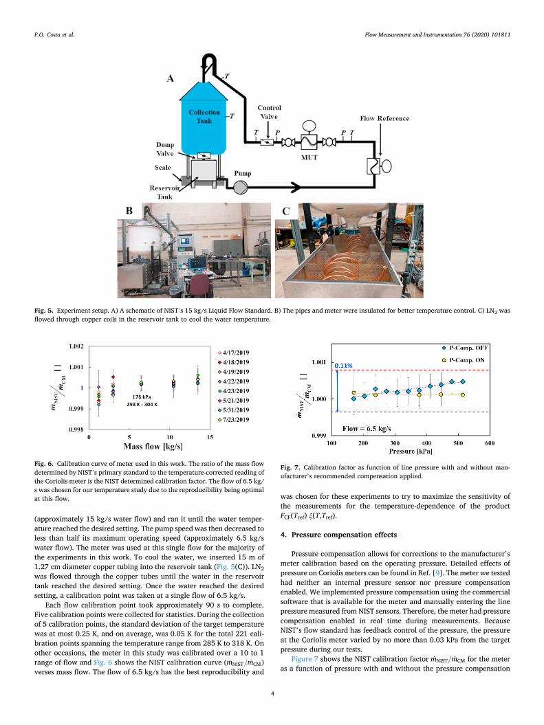
The National Institute of Standards and Technology’s (NIST) water flow calibration facility called the 15 kg/s Liquid Flow Standard (LFS) was used to test our model [8]. The LFS is a fully-automated, closed-loop system comprised of three major components: 1) a flow generation and control system, 2) a dynamic weighing system that makes SI (Interna-tional System of Units) traceable flow measurements, and 3) a test section where the meter under test is installed and calibrated. The dy-namic weighing system consists of a weigh scale and a collection tank. The scale readings are recorded at approximately 0.2 s intervals during flow accumulation into the collection tank. The time-stamped, buoy-ancy-corrected weight measurements give the mass flow. Figure 5 is a picture of the LFS.

A pump pressurizes and recirculates water through the system. The pressure at the Coriolis meter under test is controlled by a butterfly valve at the meter outlet and computer communications with a proportional- integral-derivative feedback controller. The LFS is not equipped with temperature control, therefore, we cooled the water using a liquid ni-trogen (LN2) heat exchanger and warmed the water using the heat input from the pump.

We insulated the plumbing including the meter with 1.91 cm thick “flexible rubber foam pipe insulation” with an R value of 0.53 Km2/W (Fig. 5(B)) before heating and cooling the water. To heat the water, the system’s pump was used. The pump inputs approximately 9 kW of heat when it is running at the maximum speed of 2900 revolutions per minute. Therefore, we turned the pump on at maximum speed

Fig. 2. 316 Stainless-steel elastic constants. A) Orange diamonds and blue circles are data from Refs. [1] for E(T) and G(T), respectively. The orange tri-angles and blue squares are extrapolated points from a linear fit to E(T) and G (T) data in Ref. [1] over the T range of 180 K to 295 K. The solid lines are fits to these data points. B) The red hash symbols are Poisson’s ratio calculated from E (T) and G(T) data in (A). The solid line is calculated from the lines in (A). C) The residuals of the fits to experimental data for E(T) and G(T). The error bars in (A) and (B) are the k = 2 uncertainties in E(T), G(T), and ν(T), 13.32 GPa, 4.5 GPa, and 0.015, respectively. (For interpretation of the references to colour in this figure legend, the reader is referred to the Web version of this article.)

Fig. 3. Schematic showing the basic principles of how a Coriolis meter works.

Fig. 4. Temperature-corrected mass flow is a linear function of time lag be-tween left and right pickoff sensors.

1 Vectors are shown in bold typeface.

F.O. Costa et al.

Flow Measurement and Instrumentation 76 (2020) 101811

4

(approximately 15 kg/s water flow) and ran it until the water temper-ature reached the desired setting. The pump speed was then decreased to less than half its maximum operating speed (approximately 6.5 kg/s water flow). The meter was used at this single flow for the majority of the experiments in this work. To cool the water, we inserted 15 m of 1.27 cm diameter copper tubing into the reservoir tank (Fig. 5(C)). LN2 was flowed through the copper tubes until the water in the reservoir tank reached the desired setting. Once the water reached the desired setting, a calibration point was taken at a single flow of 6.5 kg/s.

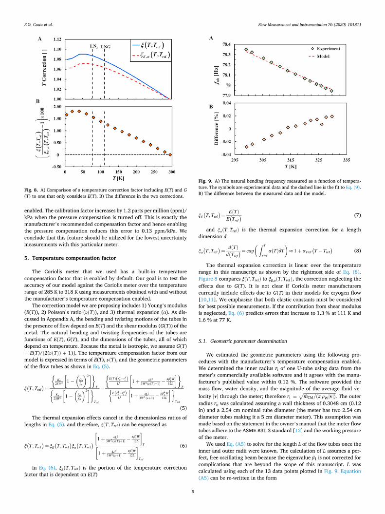
Each flow calibration point took approximately 90 s to complete. Five calibration points were collected for statistics. During the collection of 5 calibration points, the standard deviation of the target temperature was at most 0.25 K, and on average, was 0.05 K for the total 221 cali-bration points spanning the temperature range from 285 K to 318 K. On other occasions, the meter in this study was calibrated over a 10 to 1 range of flow and Fig. 6 shows the NIST calibration curve (mNIST/mCM) verses mass flow. The flow of 6.5 kg/s has the best reproducibility and

was chosen for these experiments to try to maximize the sensitivity of the measurements for the temperature-dependence of the product FCF(Tref) ξ(T,Tref).

4. Pressure compensation effects

Pressure compensation allows for corrections to the manufacturer’s meter calibration based on the operating pressure. Detailed effects of pressure on Coriolis meters can be found in Ref. [9]. The meter we tested had neither an internal pressure sensor nor pressure compensation enabled. We implemented pressure compensation using the commercial software that is available for the meter and manually entering the line pressure measured from NIST sensors. Therefore, the meter had pressure compensation enabled in real time during measurements. Because NIST’s flow standard has feedback control of the pressure, the pressure at the Coriolis meter varied by no more than 0.03 kPa from the target pressure during our tests.

Figure 7 shows the NIST calibration factor mNIST/mCM for the meter as a function of pressure with and without the pressure compensation

Fig. 5. Experiment setup. A) A schematic of NIST’s 15 kg/s Liquid Flow Standard. B) The pipes and meter were insulated for better temperature control. C) LN2 was flowed through copper coils in the reservoir tank to cool the water temperature.

Fig. 6. Calibration curve of meter used in this work. The ratio of the mass flow determined by NIST’s primary standard to the temperature-corrected reading of the Coriolis meter is the NIST determined calibration factor. The flow of 6.5 kg/ s was chosen for our temperature study due to the reproducibility being optimal at this flow.

Fig. 7. Calibration factor as function of line pressure with and without man-ufacturer’s recommended compensation applied.

F.O. Costa et al.

Flow Measurement and Instrumentation 76 (2020) 101811

5

enabled. The calibration factor increases by 1.2 parts per million (ppm)/ kPa when the pressure compensation is turned off. This is exactly the manufacturer’s recommended compensation factor and hence enabling the pressure compensation reduces this error to 0.13 ppm/kPa. We conclude that this feature should be utilized for the lowest uncertainty measurements with this particular meter.

5. Temperature compensation factor

The Coriolis meter that we used has a built-in temperature compensation factor that is enabled by default. Our goal is to test the accuracy of our model against the Coriolis meter over the temperature range of 285 K to 318 K using measurements obtained with and without the manufacturer’s temperature compensation enabled.

The correction model we are proposing includes 1) Young’s modulus (E(T)), 2) Poisson’s ratio (ν(T)), and 3) thermal expansion (α). As dis-cussed in Appendix A, the bending and twisting motions of the tubes in the presence of flow depend on E(T) and the shear modulus (G(T)) of the metal. The natural bending and twisting frequencies of the tubes are functions of E(T), G(T), and the dimensions of the tubes, all of which depend on temperature. Because the metal is isotropic, we assume G(T) = E(T)/[2(ν(T)) + 1)]. The temperature compensation factor from our model is expressed in terms of E(T), ν(T), and the geometric parameters of the flow tubes as shown in Eq. (5).

ξ(T, Tref

)=

{Ku

2SW2

[

1 −

(fnbfnt

)2]}

T{

Ku2SW2

[

1 −

(fnbfnt

)2]}

Tref

=

{E(T)(r4

o − r4i )

L3

[

1 + 4L2

3W2(ν(T)+1) −πβ4

1W12L

]}

T{E(r4

o − r4i )

L3

[

1 + 4L2

3W2(ν+1) −πβ4

1W12L

]}

Tref

(5)

The thermal expansion effects cancel in the dimensionless ratios of lengths in Eq. (5). and therefore, ξ(T,Tref) can be expressed as

ξ(T, Tref

)= ξE

(T, Tref

)ξα(T,Tref

)

[

1 + 4L2

3W2(ν(T)+1) −πβ4

1W12L

]

T[

1 + 4L2

3W2(ν+1) −πβ4

1W12L

]

Tref

(6)

In Eq. (6), ξE(T,Tref) is the portion of the temperature correction factor that is dependent on E(T)

ξE(T,Tref

)=

E(T)E(Tref

) (7)

and ξα(T,Tref) is the thermal expansion correction for a length dimension d

ξα(T, Tref

)=

d(T)d(Tref

)= exp(∫ T

Trefα(T)∂T

)

≈ 1 + αTref(T − Tref

)(8)

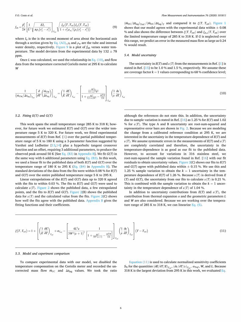
The thermal expansion correction is linear over the temperature range in this manuscript as shown by the rightmost side of Eq. (8). Figure 8 compares ξ(T,Tref) to ξE,α(T,Tref), the correction neglecting the effects due to G(T). It is not clear if Coriolis meter manufacturers currently include effects due to G(T) in their models for cryogen flow [10,11]. We emphasize that both elastic constants must be considered for best possible measurements. If the contribution from shear modulus is neglected, Eq. (6) predicts errors that increase to 1.3 % at 111 K and 1.6 % at 77 K.

5.1. Geometric parameter determination

We estimated the geometric parameters using the following pro-cedures with the manufacturer’s temperature compensation enabled. We determined the inner radius ri of one U-tube using data from the meter’s commercially available software and it agrees with the manu-facturer’s published value within 0.12 %. The software provided the mass flow, water density, and the magnitude of the average fluid ve-locity |v| through the meter; therefore ri =

mCM/(π ρW|v|)

√. The outer

radius ro was calculated assuming a wall thickness of 0.3048 cm (0.12 in) and a 2.54 cm nominal tube diameter (the meter has two 2.54 cm diameter tubes making it a 5 cm diameter meter). This assumption was made based on the statement in the owner’s manual that the meter flow tubes adhere to the ASME B31.3 standard [12] and the working pressure of the meter.

We used Eq. (A5) to solve for the length L of the flow tubes once the inner and outer radii were known. The calculation of L assumes a per-fect, free oscillating beam because the eigenvalue β1 is not corrected for complications that are beyond the scope of this manuscript. L was calculated using each of the 13 data points plotted in Fig. 9. Equation (A5) can be re-written in the form

Fig. 8. A) Comparison of a temperature correction factor including E(T) and G (T) to one that only considers E(T). B) The difference in the two corrections.

Fig. 9. A) The natural bending frequency measured as a function of tempera-ture. The symbols are experimental data and the dashed line is the fit to Eq. (9). B) The difference between the measured data and the model.

F.O. Costa et al.

Flow Measurement and Instrumentation 76 (2020) 101811

6

fnb =β2

1

2π

[1L2

EIx

πρt(r2

o − r2i)

√ ]

Tref

ξE(T, Tref

)ξα(T,Tref

)

1 + r2i ρw

/(ρt(r2

o − r2i))

√

(9)

where Ix is the is the second moment of area about the horizontal axis through a section given by Eq. (A3), ρt and ρw are the tube and internal water density, respectively. Figure 9 is a plot of fnb verses water tem-perature. The model deviates from the experimental data by 132 ± 78 ppm.

Once L was calculated, we used the relationship in Eq. (10), and flow data from the temperature corrected Coriolis meter at 295 K to calculate W

5.2. Fitting E(T) and G(T)

This work spans the small temperature range 285 K to 318 K; how-ever, for future work we estimated E(T) and G(T) over the wider tem-perature range 5 K to 320 K. For future work, we fitted experimental measurements of E(T) from Ref. [1] over the partial published temper-ature range of 5 K to 180 K using a 3-parameter function suggested by Varshni and Ledbetter [13,14] plus a hyperbolic tangent crossover function and an offset, requiring 3 additional parameters, to produce the observed peak around 50 K [See Eq. (B3) in Appendix B]. We fit G(T) in the same way with 6 additional parameters using Eq. (B3). In this work, we used a linear fit to the published data of both E(T) and G(T) over the temperature range of 180 K to 295 K (Eq. (B4) in Appendix B). The standard deviations of the data from the fits were within 0.08 % for E(T) and G(T) over the entire published temperature range 5 K to 295 K.

Linear extrapolations of the E(T) and G(T) data up to 320 K agreed with the fits to within 0.03 %. The fits to E(T) and G(T) were used to calculate ν(T). Figure 2 shows the published data, a few extrapolated points, and the fits to E(T) and G(T). Figure 2(B) shows the published data for ν(T) and the calculated value from the fits. Figure 2(C) shows how well the fits agree with the published data. Appendix B gives the fitting functions and their coefficients.

5.3. Model and experiment comparison

To compare experimental data with our model, we disabled the temperature compensation on the Coriolis meter and recorded the un-corrected mass flow mUC and Δtlag values. We took the ratio

(mUC/Δtlag)Tref /(mUC/Δtlag)T and compared it to ξ(T, Tref). Figure 1 shows that our model agrees with the experimental data within ± 0.08 % and also shows the difference between ξ(T,Tref) and ξE,α(T,Tref) over the limited temperature range of 285 K to 318 K. If G is neglected over this range, we predict an error in the measured mass flow as large as 0.24 % would result.

5.4. Model uncertainty

The uncertainty in E(T) and ν(T) from the measurements in Ref. [1] is stated in Ref. [15] to be 1.0 % and 1.5 %, respectively. We assume these are coverage factor k = 1 values corresponding to 68 % confidence level;

although the references do not state this. In addition, the uncertainty due to sample variation is stated in Ref. [16] as 1.25 % for E(T) and 1.02 % for ν(T). The type A and B uncertainty are root-sum-squared and representative error bars are shown in Fig. 2. Because we are modeling the change from a calibrated reference condition at 295 K, we are interested in the uncertainty in the temperature-dependence of E(T) and ν(T). We assume systematic errors in the measurements of E(T) and ν(T)are completely correlated and therefore, the uncertainty in the temperature-dependence is as good as our fit to the published data. However, to account for variations in 316 stainless steel, we root-sum-squared the sample variation found in Ref. [16] with our fit residuals to obtain uncertainty values. Figure 2(C) shows our fits to E(T) and G(T) agree with published data within ± 0.15 %. We use this and 1.25 % sample variation to obtain the k = 1 uncertainty in the tem-perature dependence of E(T) of 1.26 %. Because ν(T) is derived from E (T) and G(T), the uncertainty from our fits to calculate ν(T) is 0.21 %. This is combined with the sample variation to obtain the k = 1 uncer-tainty in the temperature dependence of ν(T) of 1.04 %.

In addition to uncertainty contributions from E(T) and ν(T), the contribution from thermal expansion α and the geometric parameters L and W are also considered. Because we are working over the tempera-ture range of 285 K to 318 K, we can linearize Eq. (5).

Equation (11) is used to calculate normalized sensitivity coefficients SN for the quantities (∂E/∂T/E)Tref

, (∂ν/∂T/ν)Tref, αTref , W, and L. Because

318 K is the largest deviation from 295 K in this work, we evaluated Eq.

1(mCM

/Δtlag

)

Tref

[∂

∂T

(mCM

Δtlag

)]

Tref

=

(1E

∂E∂T

)

Tref

−

⎡

⎢⎢⎣

4L2ν3(1+ν)2W2

1 + 4L2

3(1+ν)W2 −πβ4

1W12L

⎤

⎥⎥⎦

Tref

(1ν

∂ν∂T

)

Tref

(10)

ξ(T, Tref

)= 1 +

⎡

⎢⎢⎢⎣

(1E

∂E∂T

)

Tref

+αTref −

⎡

⎢⎢⎣

4L2ν3W2(ν + 1)2

1[

1 + 4L2

3W2(ν+1) −πβ4

1W12L

]

⎤

⎥⎥⎦

Tref

(1ν

∂ν∂T

)

Tref

⎤

⎥⎥⎥⎦

(T − Tref

)(11)

F.O. Costa et al.

Flow Measurement and Instrumentation 76 (2020) 101811

7

(11) at this temperature. The uncertainty in L and W was determined by comparing the values

we calculated as described above to the length of the flow tube given by the manufacturer and there is a 10.1 cm discrepancy. The total tube length is 2(L − W /2) + πW /2 or 2l+ πa, see Fig. 3. Because L goes into our total length calculation twice and W once, we assigned 2/3 of the 10.1 cm discrepancy to L and 1/3 to W. The uncertainty in αTref is

assumed to be 10 %, determined from differences observed in published values.

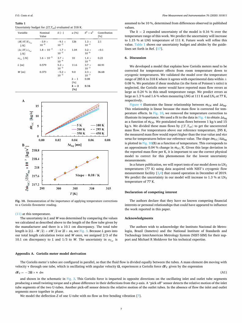
The k = 2 expanded uncertainty of the model is 0.16 % over the temperature range of this work. We predict the uncertainty will increase to 1.15 % at LNG temperature of 111 K. Future work will refine this value. Table 1 shows our uncertainty budget and abides by the guide-lines set forth in Ref. [17].

6. Discussion

We developed a model that explains how Coriolis meters need to be corrected for temperature effects from room temperature down to cryogenic temperatures. We validated the model over the temperature range of 285 K to 318 K where it agrees with experimental data within ±0.08 %. We postulate if shear modulus (in the form of Poisson’s ratio) is neglected, the Coriolis meter would have reported mass flow errors as large as 0.24 % in this small temperature range. We predict errors as large as 1.3 % and 1.6 % when measuring LNG at 111 K and LN2 at 77 K, respectively.

Figure 4 illustrates the linear relationship between mCM and Δtlag. This relationship is linear because the mass flow is corrected for tem-perature effects. In Fig. 10, we removed the temperature correction to illustrate its importance. We used a fit to the data in Fig. 4 to obtain Δtlag as a function of mCM. We postulated mass flows between 1 kg/s and 15 kg/s. We divided these mass flows by ξ(T,Tref) to get the uncorrected mass flow. For temperatures above our reference temperature, 295 K, the measured mass flow would report higher than the true value and vice versa for temperatures below our reference value. The slope ∂mUC/∂Δtlag

is plotted in Fig. 10(B) as a function of temperature. This corresponds to an approximate 0.04 % change in mUC/K. Given this large deviation in the reported mass flow per K, it is important to use the correct physical model to correct for this phenomenon for the lowest uncertainty measurements.

In a future publication, we will report tests of our model down to LN2 temperatures (77 K) using data acquired with NIST’s cryogenic flow measurement facility [3,4] that ceased operation in December of 2019. We predict the uncertainty in our model will increase to 1.3 % at LN2 temperature of 77 K.

Declaration of competing interest

The authors declare that they have no known competing financial interests or personal relationships that could have appeared to influence the work reported in this paper.

Acknowledgments

The authors wish to acknowledge the Instituto Nacional de Metro-logia, Brazil (Inmetro) and the National Institute of Standards and Technology InterAmerican Metrology System (NIST-SIM) for their sup-port and Michael R Moldover for his technical expertise.

Appendix A. Coriolis meter model derivation

The Coriolis meter’s tubes are configured in parallel, so that the fluid flow is divided equally between the tubes. A mass element dm moving with velocity v through one tube, which is oscillating with angular velocity Ω, experiences a Coriolis force dFC given by the expression

dFC = − 2Ω × v dm (A1)

and shown in the schematic in Fig. 3. This Coriolis force is imparted in opposite directions on the oscillating inlet and outlet tube segments producing a small twisting torque and a phase difference in their deflections from the y-axis. A “pick off” sensor detects the relative motion of the inlet tube segments of the two U-tubes. Another pick-off sensor detects the relative motion of the outlet tubes. In the absence of flow the inlet and outlet segments move together in phase.

We model the deflection Z of one U-tube with no flow as free bending vibration [7].

Fig. 10. Demonstration of the importance of applying temperature corrections to a Coriolis flowmeter reading.

Table 1 Uncertainty budget for ξ(T,Tref) evaluated at 318 K.

Variable Nominal Value

S [− ] u [%] S2 × u2 Contribution [%]

(∂E/∂T/E)Tref

[/K] − 3.9 ×10− 4

− 9.1 ×10− 3

126 1.3 ×10− 4

2.1

(∂ν/∂T/ν)Tref

[/K] 1.8 × 10− 4 − 1.7 ×

10− 3 1.04 3.2 ×

10− 6 <0.1

αTref [/K] 1.6 × 10− 5 3.7 ×10− 4

10 1.4 ×10− 5

0.23

L [m] 0.579 5.2 ×10− 3

11.6 3.7 ×10− 3

60.91

W [m] 0.373 − 5.2 ×10− 3

9.0 2.3 ×10− 3

36.68

k = 1 [%]

0.08

k ¼ 2 [%]

0.16

F.O. Costa et al.

Flow Measurement and Instrumentation 76 (2020) 101811

8

Ix =π4(r4

o − r4i

)(A2)

where E is Young’s modulus, Ix is the second moment of area about the horizontal axis through a section given by

Ix =π4(r4

o − r4i

)(A3)

and λ is the linear density of a tube and the water inside given by

λ= π(ρt(r2

o − r2i

)+ ρwr2

i

)(A4)

In Eq. (A3) and Eq. (A4), ro and ri are the outer and inner radii of the flow tubes, respectively, ρt and ρw are the tube and internal water density, respectively. The solution to Eq. (A2) for the tube’s fundamental vibration exists for the frequency

fnb =1

2π

(β1

L

)2EIx

λ

√

(A5)

The numeric constant β1 ≅ 1.8751 is the first order solution to the cantilever beam mathematical model [7] and L is the length of the flow tubes plus the U bend radius (l + a), see Fig. 3.

In free twisting motion about the y-axis, the U-tubes have a natural twisting frequency, fnt. However, mass flowing through the U-tubes driven at the natural bending frequency, fnb, creates a twisting motion at the same frequency, which is significantly below fnt. The twisting motion produces a phase shift between the left and right pickoffs. The phase shift is conveniently expressed as a time lag, Δtlag, which is directly proportional to the mass flow m.

The equation of motion for twisting, due to the Coriolis force arising from mass flow, is

Iy∂2θ∂t2 +Kuθ = 2SΩmlW (A6)

where Iy is the moment of inertia about the y-axis, given by

Iy =π2W3

16[ρt(r2

o − r2i

)+ ρwr2

i

](A7)

θ is the angle of twist about the y-axis, Ku is the spring constant for twisting, S is a shape parameter, m is the mass flow through the Coriolis meter, l is the “straight” length of the inlet and outlet tube segments, W is the distance between the inlet and outlet tube segments, and Ω is the magnitude of the driven angular velocity of the bending motion, given by

Ω=Ω0 cos(2πfnbt) (A8)

In Eq. (A8), Ω0 is the amplitude of the driven angular velocity. The homogeneous twist equation (Eq. (A6) with the right hand side set to zero) has a solution of the form θ(t)∝exp(i2πft) if the frequency equals the

natural twist frequency fnt given by

fnt =1

2π

Ku

Iy

√

(A9)

The spring constant for twisting Ku can be further reduced to

Ku =JL

G +3IxW2

4L3 E (A10)

where G is the shear modulus and J is the polar 2nd moment of area about z-axis given by

J =π2(r4

o − r4i

)(A11)

The motion involves both bending and twisting of the tubes. The first term on the right hand side of Eq. (A10) models the pure twisting and the second term models the pure bending of the flow tube(s). Both E and G are temperature dependent. With Δtlag calculated from

Δtlag =displacement between corners

velocity of corners=

WθlΩ

(A12)

we can calculate the mass flow through one tube

m=Ku

2SW2

[

1 −(

fnb

fnt

)2]

Δtlag (A13)

Appendix B. Fitting function for E(T) and G(T)

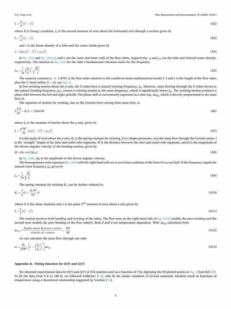
We obtained experimental data for E(T) and G(T) of 316 stainless steel as a function of T by digitizing the 59 plotted points in Fig. 2 from Ref. [1]. To fit the data from 5 K to 180 K, we followed Ledbetter [14], who fit the elastic constants of several austenitic stainless steels as functions of temperature using a theoretical relationship suggested by Varshni [13].

F.O. Costa et al.

Flow Measurement and Instrumentation 76 (2020) 101811

9

CE,G(T)=C0 −d

eT0/T − 1(B1)

where CE,G represents either E or G in gigapascals, C0, d and T0 are adjustable parameters, and T is in Kelvin. Because Eq. (B1) does not reproduce the observed low-temperature anomaly for E(T) and G(T) in 316 stainless steel, we added a crossover function

defined by

ΔCE,G(T)= c[tanh[b(T − Ts)] − 1] (B2)

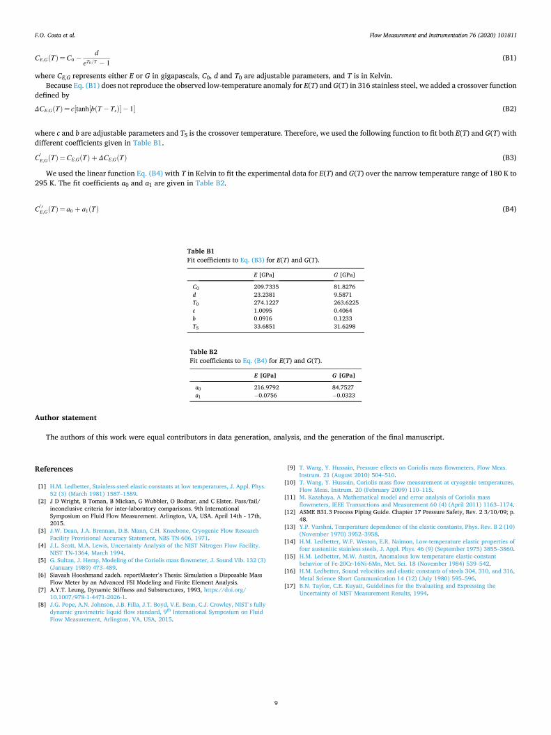
where c and b are adjustable parameters and TS is the crossover temperature. Therefore, we used the following function to fit both E(T) and G(T) with different coefficients given in Table B1.

C′

E,G(T)=CE,G(T) + ΔCE,G(T) (B3)

We used the linear function Eq. (B4) with T in Kelvin to fit the experimental data for E(T) and G(T) over the narrow temperature range of 180 K to 295 K. The fit coefficients a0 and a1 are given in Table B2.

C′ ′E,G(T)= a0 + a1(T) (B4)

Table B1 Fit coefficients to Eq. (B3) for E(T) and G(T).

E [GPa] G [GPa]

C0 209.7335 81.8276 d 23.2381 9.5871 T0 274.1227 263.6225 c 1.0095 0.4064 b 0.0916 0.1233 TS 33.6851 31.6298

Table B2 Fit coefficients to Eq. (B4) for E(T) and G(T).

E [GPa] G [GPa]

a0 216.9792 84.7527 a1 − 0.0756 − 0.0323

Author statement

The authors of this work were equal contributors in data generation, analysis, and the generation of the final manuscript.

References

[1] H.M. Ledbetter, Stainless-steel elastic constants at low temperatures, J. Appl. Phys. 52 (3) (March 1981) 1587–1589.

[2] J D Wright, B Toman, B Mickan, G Wubbler, O Bodnar, and C Elster. Pass/fail/ inconclusive criteria for inter-laboratory comparisons. 9th International Symposium on Fluid Flow Measurement. Arlington, VA, USA. April 14th - 17th, 2015.

[3] J.W. Dean, J.A. Brennan, D.B. Mann, C.H. Kneebone, Cryogenic Flow Research Facility Provisional Accuracy Statement, NBS TN-606, 1971.

[4] J.L. Scott, M.A. Lewis, Uncertainty Analysis of the NIST Nitrogen Flow Facility. NIST TN-1364, March 1994.

[5] G. Sultan, J. Hemp, Modeling of the Coriolis mass flowmeter, J. Sound Vib. 132 (3) (January 1989) 473–489.

[6] Siavash Hooshmand zadeh. reportMaster’s Thesis: Simulation a Disposable Mass Flow Meter by an Advanced FSI Modeling and Finite Element Analysis.

[7] A.Y.T. Leung, Dynamic Stiffness and Substructures, 1993, https://doi.org/ 10.1007/978-1-4471-2026-1.

[8] J.G. Pope, A.N. Johnson, J.B. Filla, J.T. Boyd, V.E. Bean, C.J. Crowley, NIST’s fully dynamic gravimetric liquid flow standard, 9th International Symposium on Fluid Flow Measurement, Arlington, VA, USA, 2015.

[9] T. Wang, Y. Hussain, Pressure effects on Coriolis mass flowmeters, Flow Meas. Instrum. 21 (August 2010) 504–510.

[10] T. Wang, Y. Hussain, Coriolis mass flow measurement at cryogenic temperatures, Flow Meas. Instrum. 20 (February 2009) 110–115.

[11] M. Kazahaya, A Mathematical model and error analysis of Coriolis mass flowmeters, IEEE Transactions and Measurement 60 (4) (April 2011) 1163–1174.

[12] ASME B31.3 Process Piping Guide. Chapter 17 Pressure Safety, Rev. 2 3/10/09; p. 48.

[13] Y.P. Varshni, Temperature dependence of the elastic constants, Phys. Rev. B 2 (10) (November 1970) 3952–3958.

[14] H.M. Ledbetter, W.F. Weston, E.R. Naimon, Low-temperature elastic properties of four austenitic stainless steels, J. Appl. Phys. 46 (9) (September 1975) 3855–3860.

[15] H.M. Ledbetter, M.W. Austin, Anomalous low temperature elastic-constant behavior of Fe-20Cr-16Ni-6Mn, Met. Sci. 18 (November 1984) 539–542.

[16] H.M. Ledbetter, Sound velocities and elastic constants of steels 304, 310, and 316, Metal Science Short Communication 14 (12) (July 1980) 595–596.

[17] B.N. Taylor, C.E. Kuyatt, Guidelines for the Evaluating and Expressing the Uncertainty of NIST Measurement Results, 1994.

F.O. Costa et al.