Flow noise response of a diaphragm based fibre laser hydrophone array

Unnikrishnan Kuttan Chandrikaa,∗, Venugopalan Pallayila, Kian Meng Limb, Chye Heng Chewb

aAcoustic Research Laboratory, National University of Singapore, SingaporebMechanical Engineering Department, National University of Singapore, Singapore

Abstract

Flow noise is one of the factors limiting the performance of towed array systems, especially thin-

line arrays. Response of a fibre laser hydrophone array to axisymmetric boundary layer wall

pressure excitation is presented. A simplified theoretical model is obtained to predict the flow

noise levels inside fluid filled towed arrays. An axisymmetric wall pressure model was used along

with frequency-wavenumber transfer characteristics obtained from finite element analysis (FEA)

to arrive at flow noise estimates under normal operating speeds. The results were then compared

with internal pressure spectra obtained from the simplified theoretical model. The flow noise levels

corresponding to operating tow speeds below 2 m/s for the analysed configuration is found to be

lower than the nominal low-level ambient noise floor observed in the sea for frequencies greater

than 200Hz. The results show that the flow noise isolation achieved through fluid filled array

construction reduces with increase in tow speed.

Keywords: Flow noise, Fibre laser hydrophone, Towed array sonar

1. Introduction

Traditionally, piezo-ceramic based hydrophones are used in towed array construction; however,

recently fibre laser based technology has emerged as an alternative solution (Hill et al., 1999; Foster

et al., 2012). Fibre lasers eliminate the need for electronics in the wet-end of the sensor array.

Their inherent advantages like high sensitivity to strain, ease of multiplexing, intrinsic safety to

water, and remote monitoring capability and thin-line nature (Hill et al., 1998; Batchellor and

Edge, 1990) make fibre laser based sensing a suitable candidate for construction of thin-line towed

arrays.

The application of thin-line towed arrays for underwater surveillance to some extent is lim-

∗Corresponding authorEmail address: unni@arl.nus.edu.sg (Unnikrishnan Kuttan Chandrika)

Preprint submitted to Ocean Engineering September 3, 2014

ited by the noise generated due to turbulent boundary layer (TBL) pressure fluctuations, usually

referred as flow noise in literature. Flow noise has a direct dependence on the tow speed with

detrimental effect on the achievable signal to noise ratio (SNR) of the sensor system. Magnitudes

of these wall pressure fluctuations are also expected to increase with reduction in the towed ar-

ray diameter (Chase, 1981; Tutty, 2008). Thus, flow noise is one of the major considerations in

estimating the performance of thin-line towed arrays.

Flow noise calculations for towed arrays require an adequate statistical model of wall pressure

fluctuations, knowledge of frequency-wavenumber transfer function of the towed array packaging,

response characteristics of the sensor, and filtering characteristics of the array processing algo-

rithms. Carpenter and Kewley (1983) presented one of the early results on flow noise response of

a fluid filled towed array. Their study employed a simple mechanical transfer function to model

array packaging. They observed that the predicted internal noise levels were lower than the exper-

imentally measured values. Similar procedure was employed by Knight (1996) to study the flow

noise filtering by a group of hydrophones. However, this study was also limited by the elementary

transfer function used to model the wavenumber filtering by the fluid filled towed array packaging.

There have been many attempts in the past to improve upon the models of frequency-wavenumber

transfer characteristics of fluid filled towed arrays (Francis et al., 1984; Dowling, 1998). In all these

studies, either the effect of sensors were neglected or the sensors were considered as line elements

or infinite cylinders located along the axis of the array.

The fibre laser hydrophone considered in this study consists of a fibre laser sensor mounted

centrally on a diaphragm. The diaphragm helps in achieving the required sensitivity values by

amplifying the strain on the fibre laser and its orientation is normal to the axis of the towed

array. Hence, the averaging effect on flow noise due to the finite size of the sensor along its axis

is minimal in these diaphragm based sensors. Thus a different approach to the analysis for flow

noise estimation is necessary.

In this paper a finite element analysis based procedure to estimate the flow noise levels experi-

enced by the fibre laser sensors packaged in a fluid filled elastomer cylinder is presented. The results

are then compared with the predictions from a simplified analytical model of a submerged fluid

filled infinite cylinder. The paper is organised into three main sections. The array configuration

and sensor details are presented in section 2, followed by the analytical model and finite element

analysis procedure in section 3. Results and discussions are presented in section 4, followed by

2

summary of findings and conclusions.

2. Fibre Laser Hydrophone Array

Fibre lasers are Fabry-Perot resonance cavities created on an active fibre (rare earth element

doped fibre) by writing spectrally matched Bragg gratings. They absorb the light energy from an

external pump source and generate laser at wavelengths which depend on the grating pitch, effective

refractive index of the resonance cavity and emission bandwidth of the dopant used in the active

fibre. Any changes in the grating structure due to external excitations like strain or temperature

will result in corresponding changes in the fibre laser output wavelength. Multiple fibre lasers

can be connected on a single optical fibre line using wavelength division multiplexing scheme

through careful design of grating structure of individual fibre lasers. Interferometric systems along

with phase demodulators are usually employed to convert the fibre laser wavelength changes into

electrical signals. Detailed review of the operating principles of a fibre laser sensors and associated

interferometric techniques can be found in Hill et al. (1999) and Kirkendall and Dandridge (2004).

Although the wavelength of the fibre laser output is highly sensitive to external excitations

like strain, a high elastic modulus of silica glass necessitate additional arrangements to achieve

required sensitivity values. The sensor configuration used in the construction of the array is shown

in Figure 1. A distributed feedback fibre laser (DFB-FL) is centrally placed inside an aluminium

packaging with one end of the fibre attached to a metallic diaphragm and the other end to a

pre-tensioning arrangement. The diaphragm amplifies the strain on the fibre laser to achieve

the required sensitivity. The cavity behind the diaphragm is filled with air and proper sealing

is provided on the sensor shell to prevent water ingress into the sensor. More details on the

sensor construction and its performance characteristics can be found in Kuttan Chandrika et al.

(2013). A water filled polyurethane tube inside which individual hydrophones are assembled, as

shown in Figure 1, is considered in this study. The polyurethane tube helps in streamlining the

flow and isolates the sensors from hydrodynamic disturbances in the turbulent boundary layer.

Furthermore, it serves as a wavenumber filter to reduce the flow noise experienced by the sensors.

3. Theory

Two major parameters that determine the flow noise response of a fibre laser hydrophone

packaged inside the array tube are the frequency-wavenumber response of the sensor in packaged

3

Figure 1: Schematics of sensor and array configurations

condition denoted by H(k, ω) and the spectra of the wall pressure excitation P (k, ω). The flow

noise response of the sensor in the array could be expressed as (Carpenter and Kewley (1983)).

Q(ω) =

∫ ∞−∞

P (k, ω)|H(k, ω)|2dk (1)

where k is the wavenumber and ω is the angular frequency.

3.1. Flow noise model

The wall pressure fluctuations in a turbulent boundary layer are random in nature. Calculation

of the response of a structure to these pressure fluctuations requires a valid statistical description

of wall pressure field in frequency-wavenumber or time-space domain. Experimental results re-

ported by many researchers showed that the wall pressure field consisted of a broad spectrum of

wavenumber components that changes slowly with time in a reference frame that moves along with

the flow (Bull, 1996). Another observed feature of the wall pressure spectrum is the concentration

of the flow noise energy near a wavenumber kc = ω/Uc, arising due to the convection of pressure

field in the boundary layer at a convection velocity Uc. This convection velocity depends on the

mean stream-wise velocity at locations of eddies that are major contributors to the turbulent pres-

sure field (Foley et al., 2011). The concentration of flow noise energy near the convection velocity

leads to a ridge like feature in the frequency-wavenumber spectrum usually referred as “convective

4

ridge” in the literature (see Figure 2).

One of the successful early attempts on modelling wall pressure spectra was by Corcos (1967)

and his model was based on the narrowband spatial correlations of wall pressures on a flat plate.

As per Corcos model, the spatial correlation function can be written as

Γ(ω, ξ1, ξ2) = φ(ω) exp

(−α|ωξ1

Uc| − β|ωξ2

Uc|+ iωξ1

Uc

), (2)

where ξ1 and ξ2 are the spatial separations along and normal to the flow direction respectively. α

and β are the decay constants in exponential decrease of correlation with spatial separation. Uc is

the convection velocity and it has a magnitude of the order of flow velocity. Frequency-wavenumber

spectrum obtained by Fourier transform of equation (2), with parameter values estimated from

curve fitting the experimental results, was used by Ko and Nuttall (1991) and Ko (1993) for flow

noise calculations. Though the model gives a satisfactory prediction of the wall pressure spectra

in the “convective ridge” where majority of the flow noise energy is concentrated , it over-predicts

the levels corresponding to low and high wavenumber regions. The response peak for sensor and

array packaging usually correspond to excitations by the components with phase velocities that

matches the structural wave speeds. Hence, the response peaks can fall in a region corresponding

toω

kz> Uc where kz is the wavenumber along the flow. A comparative study on various TBL wall

pressure models by Graham (1997) concluded that models that give more accurate representation

of frequency-wavenumber spectrum at convective and sub-convective wave numbers are needed in

such situations.

Chase (1980) presented a semi-empirical model which gave improved predictions of of wall

pressure frequency-wavenumber spectra in convective and sub-convective regions. He modified

it again in 1987 to include the effects of compressibility (Chase, 1987). Ciappi et al. (2009)

demonstrated the applicability of Chase model for the response prediction of flat plates under

TBL wall pressure excitations.

Many of the observed structural features of the cylindrical boundary layer are similar to those

observed in flat plate turbulent boundary layers. However, the turbulence intensities for cylin-

der are lower than that for a flat plate case for most of the boundary layer (outer regions) as the

smaller surface area of the cylinder limits the amount of vorticity introduced in to the fluid (Snarski

and Lueptow, 1995). The applicability of Chase flat plate model for prediction of axisymmetric

boundary layer wall pressures was demonstrated by Foley et al. (2011) based on wall pressure mea-

5

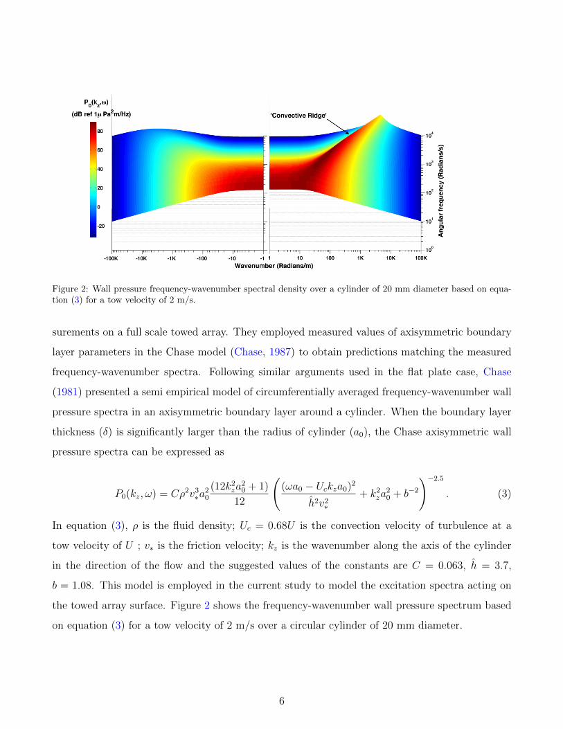
Figure 2: Wall pressure frequency-wavenumber spectral density over a cylinder of 20 mm diameter based on equa-tion (3) for a tow velocity of 2 m/s.

surements on a full scale towed array. They employed measured values of axisymmetric boundary

layer parameters in the Chase model (Chase, 1987) to obtain predictions matching the measured

frequency-wavenumber spectra. Following similar arguments used in the flat plate case, Chase

(1981) presented a semi empirical model of circumferentially averaged frequency-wavenumber wall

pressure spectra in an axisymmetric boundary layer around a cylinder. When the boundary layer

thickness (δ) is significantly larger than the radius of cylinder (a0), the Chase axisymmetric wall

pressure spectra can be expressed as

P0(kz, ω) = Cρ2v3∗a20

(12k2za20 + 1)

12

((ωa0 − Uckza0)2

h2v2∗+ k2za

20 + b−2

)−2.5. (3)

In equation (3), ρ is the fluid density; Uc = 0.68U is the convection velocity of turbulence at a

tow velocity of U ; v∗ is the friction velocity; kz is the wavenumber along the axis of the cylinder

in the direction of the flow and the suggested values of the constants are C = 0.063, h = 3.7,

b = 1.08. This model is employed in the current study to model the excitation spectra acting on

the towed array surface. Figure 2 shows the frequency-wavenumber wall pressure spectrum based

on equation (3) for a tow velocity of 2 m/s over a circular cylinder of 20 mm diameter.

6

3.2. Analytical model

A good insight into the frequency-wavenumber response characteristics of a fluid filled towed

array can be obtained from the analysis of an infinite fluid filled tube excited by TBL pressure

fluctuations. The array tube can be modelled as an isotropic shell. A fluid loading term can be used

to model the effect of the inside and outside fluid on the response of the tube. In the absence of

external moments on shell, the fluid loading term can be derived from the pressure loads acting on

the shell from internal and external fluids. These pressure loads from the fluids can be obtained by

equating normal velocities at the fluid structure interfaces followed by the application of boundary

condition related to the pressure gradient at the interface. Following a detailed derivation given

in reference Skelton and James (1997), the equations of motion after Fourier transform can be

written in terms of spectral field quantities as in Eq. (4).

[S] [u]

=[F]

(4a)

where

[S]

=

S11(n, kz) S12(n, kz) S13(n, kz)

S21(n, kz) S22(n, kz) S23(n, kz)

S31(n, kz) S32(n, kz) S33(n, kz) + fl

, (4b)

[u]

=

uz(n, kz)

uφ(n, kz)

ur(n, kz)

,[F]

=

Fz(n, kz)

Fφ(n, kz)

Fr(n, kz)

, (4c)

7

S11(n, kz) = −E1

(k2z + n21− ν

2a2

)− ω2ρsh, (4d)

S12(n, kz) =−E1(1 + ν)nkz

2a, (4e)

S13(n, kz) =−E1νikz

a, (4f)

S21(n, kz) = S12(n, kz), (4g)

S22(n, kz) = E1

((1− ν)k2z

2+n2

a2+ 2k2zΛ

2(1− ν) +Λ2n2

a2

)− ω2ρsh, (4h)

S23(n, kz) = −E1

(in

a2+ iΛ2(2− ν)k2zn+

iΛ2n3

a2

)(4i)

S31(n, kz) = −S13(n, kz), (4j)

S32(n, kz) = −S23(n, kz), (4k)

S33(n, kz) = E1

(1

a2+ Λ2a2k4z +

Λ2n4

a2+ 2Λ2k2zn

2

)− ω2ρsh, (4l)

fl = ρω2ur(n, kz)H|n|(γa)

γH|n|′(γa)

− ρω2ur(n, kz)J|n|(γa)

γJ|n|′(γa)

, (4m)

Λ2 =h2

12a2, (4n)

E1 =Eh

1− ν2, (4o)

γ =

√(k0

2 − kz2), k0 = ω/c. (4p)

In equation (4) uz(n, kz), ur(n, kz) and uφ(n, kz) are the spectral displacements and Fz(n, kz),

Fφ(n, kz), and Fr(n, kz) are the spectral excitations in cylindrical coordinate system along direc-

tions denoted by the subscripts. E, ν, ρs are the Young’s modulus, Poisson’s ratio and density

respectively of the tube material and c is the speed of sound in water and ρ is the density of water.

a is the mean radius of the tube and h is the tube thickness. In equation (4m) Jn and Hn are the

Bessel and Hankel functions of first kind with order n. n represents the wavenumber along the

circumference of the cylinder and takes only integer values. For the problem at hand, n=0 as we

are interested in the axisymmetric part of the solution.

The centre line pressure should be finite and normal velocities should be equal at fluid structure

interface. Applying these conditions, the equation for the pressure inside the array tube can be

8

written as

pi(r, n, kz) = ρω2ur(n, kz)J|n|(γr)

γJ|n|′(γa)

(5)

where r is the radial location of the observation point inside the array tube.

A relation between the external radial excitation and internal pressure can be obtained from

equations (4a) and (5). Multiplying both sides of Eq. (4a) with[Ψ]

=[S]−1

yields

[u]

=[Ψ] [F]. (6)

Multiplying Eq. (6) with[u]∗

, where ∗ represents the Hermitian operation, yields

[u] [u]∗

=[Ψ] [F] [F]∗[

Ψ]∗. (7)

It can be assumed that the external excitation is primarily radial in nature and arise from the

normal wall pressure acting at the external surfaces of the cylinder. As Fz(n, kz), Fφ(n, kz) = 0 ,

Eq. (7) gives

urur∗ = Ψ33Ψ33

∗P0(kz) (8)

The power spectral density of the internal pressure at any radial location for an axisymmetric

problem can be derived using relations given in equations (5) and (8) and can be expressed as

Pi(ω) =

∫ρ2ω4

∣∣∣Ψ33

∣∣∣2 ∣∣∣∣ J0(γr)

γ1J0′(γa)

∣∣∣∣2 P0(kz, ω)dkz. (9)

3.3. Frequency-wavenumber response spectra : FEA

The analytical model derived in the section 3.2 is highly simplified and completely neglects

the presence of sensors in the tube. The presence of sensors could introduce changes in acoustic

modes leading to corresponding variations in predictions on flow noise response of the fluid filled

arrays. Analytical representation of the response characteristics for the actual array and sensor

configuration is difficult due to the complex geometrical and structural features. Hence a finite

element analysis technique is used to obtain the frequency-wavenumber response characteristics of

the sensor packaged in a fluid filled towed array tube.

Mode based random response analysis, which is an extension of mode based dynamic analysis

9

using random process theory, is one of the most widely used approaches in estimation of structural

response to TBL wall pressure excitations. But a dense fluid loading and high structural damping,

as in the present case, will lead to modal coupling (Leehey, 1988; Franco et al., 2013). Hence

a direct frequency domain dynamic analysis procedure is used in the current study to obtain

the frequency-wavenumber response characteristics of the sensor array. An axisymmetric analysis

procedure is employed considering the axisymmetric nature of geometry and loading, leading to

significant reduction in computational size of the problem.

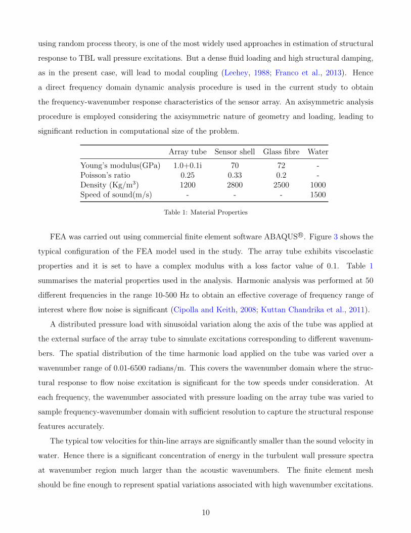
Array tube Sensor shell Glass fibre Water

Young’s modulus(GPa) 1.0+0.1i 70 72 -Poisson’s ratio 0.25 0.33 0.2 -Density (Kg/m3) 1200 2800 2500 1000Speed of sound(m/s) - - - 1500

Table 1: Material Properties

FEA was carried out using commercial finite element software ABAQUS R©. Figure 3 shows the

typical configuration of the FEA model used in the study. The array tube exhibits viscoelastic

properties and it is set to have a complex modulus with a loss factor value of 0.1. Table 1

summarises the material properties used in the analysis. Harmonic analysis was performed at 50

different frequencies in the range 10-500 Hz to obtain an effective coverage of frequency range of

interest where flow noise is significant (Cipolla and Keith, 2008; Kuttan Chandrika et al., 2011).

A distributed pressure load with sinusoidal variation along the axis of the tube was applied at

the external surface of the array tube to simulate excitations corresponding to different wavenum-

bers. The spatial distribution of the time harmonic load applied on the tube was varied over a

wavenumber range of 0.01-6500 radians/m. This covers the wavenumber domain where the struc-

tural response to flow noise excitation is significant for the tow speeds under consideration. At

each frequency, the wavenumber associated with pressure loading on the array tube was varied to

sample frequency-wavenumber domain with sufficient resolution to capture the structural response

features accurately.

The typical tow velocities for thin-line arrays are significantly smaller than the sound velocity in

water. Hence there is a significant concentration of energy in the turbulent wall pressure spectra

at wavenumber region much larger than the acoustic wavenumbers. The finite element mesh

should be fine enough to represent spatial variations associated with high wavenumber excitations.

10

Thus mesh resolution required in the current analysis are much finer than the ones typically used

in conventional acoustic analysis. The meshing scheme used in the analysis ensured at least 6

elements per wavenumber even at the highest wavenumber considered in the current study and

this led to a nodal spacing of 0.15 mm at the array tube for a 6500 radians/m loading.

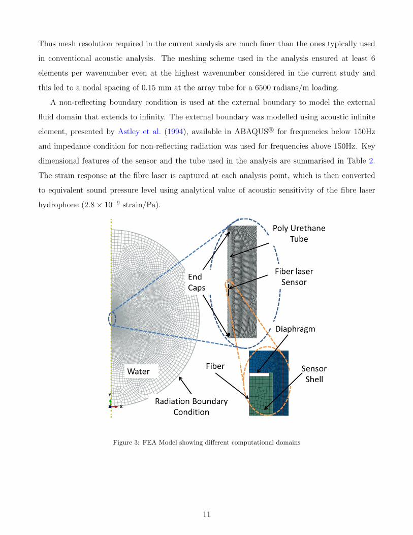
A non-reflecting boundary condition is used at the external boundary to model the external

fluid domain that extends to infinity. The external boundary was modelled using acoustic infinite

element, presented by Astley et al. (1994), available in ABAQUS R© for frequencies below 150Hz

and impedance condition for non-reflecting radiation was used for frequencies above 150Hz. Key

dimensional features of the sensor and the tube used in the analysis are summarised in Table 2.

The strain response at the fibre laser is captured at each analysis point, which is then converted

to equivalent sound pressure level using analytical value of acoustic sensitivity of the fibre laser

hydrophone (2.8× 10−9 strain/Pa).

Figure 3: FEA Model showing different computational domains

11

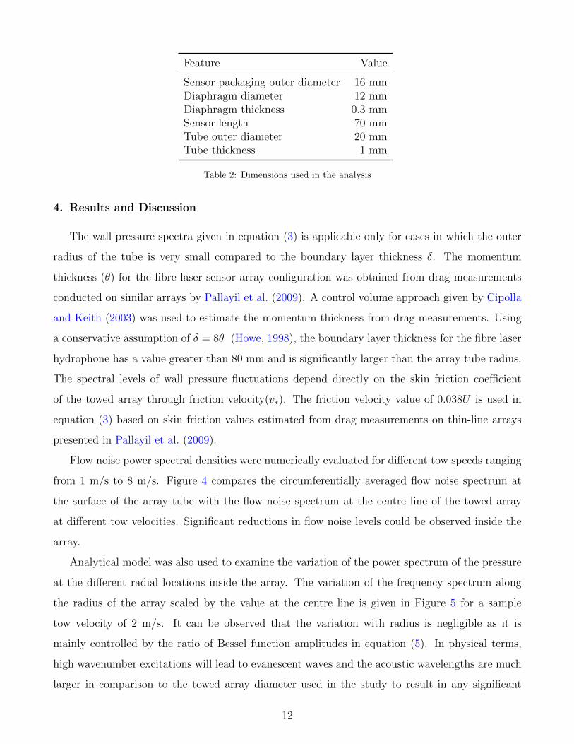
Feature Value

Sensor packaging outer diameter 16 mmDiaphragm diameter 12 mmDiaphragm thickness 0.3 mmSensor length 70 mmTube outer diameter 20 mmTube thickness 1 mm

Table 2: Dimensions used in the analysis

4. Results and Discussion

The wall pressure spectra given in equation (3) is applicable only for cases in which the outer

radius of the tube is very small compared to the boundary layer thickness δ. The momentum

thickness (θ) for the fibre laser sensor array configuration was obtained from drag measurements

conducted on similar arrays by Pallayil et al. (2009). A control volume approach given by Cipolla

and Keith (2003) was used to estimate the momentum thickness from drag measurements. Using

a conservative assumption of δ = 8θ (Howe, 1998), the boundary layer thickness for the fibre laser

hydrophone has a value greater than 80 mm and is significantly larger than the array tube radius.

The spectral levels of wall pressure fluctuations depend directly on the skin friction coefficient

of the towed array through friction velocity(v∗). The friction velocity value of 0.038U is used in

equation (3) based on skin friction values estimated from drag measurements on thin-line arrays

presented in Pallayil et al. (2009).

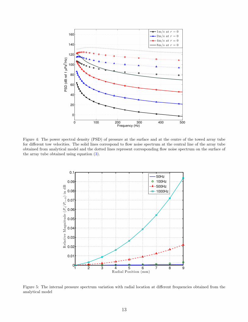
Flow noise power spectral densities were numerically evaluated for different tow speeds ranging

from 1 m/s to 8 m/s. Figure 4 compares the circumferentially averaged flow noise spectrum at

the surface of the array tube with the flow noise spectrum at the centre line of the towed array

at different tow velocities. Significant reductions in flow noise levels could be observed inside the

array.

Analytical model was also used to examine the variation of the power spectrum of the pressure

at the different radial locations inside the array. The variation of the frequency spectrum along

the radius of the array scaled by the value at the centre line is given in Figure 5 for a sample

tow velocity of 2 m/s. It can be observed that the variation with radius is negligible as it is

mainly controlled by the ratio of Bessel function amplitudes in equation (5). In physical terms,

high wavenumber excitations will lead to evanescent waves and the acoustic wavelengths are much

larger in comparison to the towed array diameter used in the study to result in any significant

12

0 100 200 300 400 500

0

20

40

60

80

100

120

140

160

Frequency (Hz)

PS

D (

dB

re

f 1

µP

a2/H

z)

1m/s at r = 0

2m/s at r = 0

4m/s at r = 0

8m/s at r = 0

Figure 4: The power spectral density (PSD) of pressure at the surface and at the centre of the towed array tubefor different tow velocities. The solid lines correspond to flow noise spectrum at the central line of the array tubeobtained from analytical model and the dotted lines represent corresponding flow noise spectrum on the surface ofthe array tube obtained using equation (3).

1 2 3 4 5 6 7 8 90

0.01

0.02

0.03

0.04

0.05

0.06

0.07

0.08

0.09

0.1

Radial Position (mm)

RelativeMagnitude(P

r/P

r=0)in

dB

50Hz

100Hz

500Hz

1000Hz

Figure 5: The internal pressure spectrum variation with radial location at different frequencies obtained from theanalytical model

13

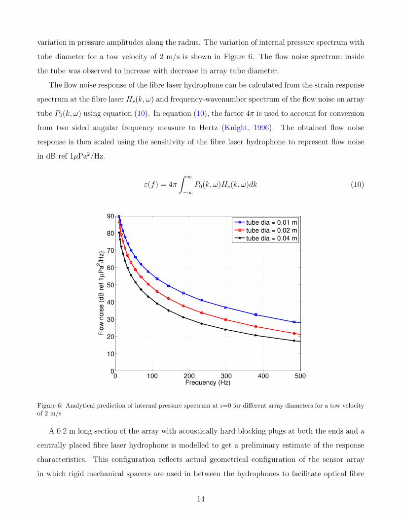
variation in pressure amplitudes along the radius. The variation of internal pressure spectrum with

tube diameter for a tow velocity of 2 m/s is shown in Figure 6. The flow noise spectrum inside

the tube was observed to increase with decrease in array tube diameter.

The flow noise response of the fibre laser hydrophone can be calculated from the strain response

spectrum at the fibre laser Hs(k, ω) and frequency-wavenumber spectrum of the flow noise on array

tube P0(k, ω) using equation (10). In equation (10), the factor 4π is used to account for conversion

from two sided angular frequency measure to Hertz (Knight, 1996). The obtained flow noise

response is then scaled using the sensitivity of the fibre laser hydrophone to represent flow noise

in dB ref 1µPa2/Hz.

ε(f) = 4π

∫ ∞−∞

P0(k, ω)Hs(k, ω)dk (10)

0 100 200 300 400 5000

10

20

30

40

50

60

70

80

90

Frequency (Hz)

Flo

w n

ois

e (

dB

re

f 1

µP

a2/H

z)

tube dia = 0.01 m

tube dia = 0.02 m

tube dia = 0.04 m

Figure 6: Analytical prediction of internal pressure spectrum at r=0 for different array diameters for a tow velocityof 2 m/s

A 0.2 m long section of the array with acoustically hard blocking plugs at both the ends and a

centrally placed fibre laser hydrophone is modelled to get a preliminary estimate of the response

characteristics. This configuration reflects actual geometrical configuration of the sensor array

in which rigid mechanical spacers are used in between the hydrophones to facilitate optical fibre

14

splicing and its routing. This model consisted of 1.2 million degrees of freedom at the highest

wavenumber considered in the analysis. Moreover the dynamic analysis step needs to be repeated

6250 times to effectively sample the frequency-wavenumber domain considered in the study. The

analysis took a CPU time of more than 7 hours on an Intel Xeon R© W3530 (2.8GHz, quad core)

Linux workstation with 12 GB RAM. Thin-line arrays used in underwater surveillance application

usually consists of many individual sensors spaced inside the array based on array signal processing

requirements and can have lengths of the order of a few tens of meters. Modelling the entire

array for its response characteristics is computationally expensive as the fine mesh resolution

requirements arising from the presence of significant energy concentration at high wavenumber

regions in the turbulent wall pressure spectra.

10−2 10

0 102 10

4

101

102

103

−280

−260

−240

−220

−200

−180

−160

wavenumber (rad/m)

Fre

quency (H

z)

Str

ain

Response d

B r

ef 1 s

train

/Pa)

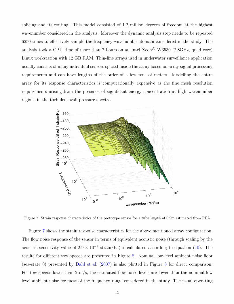
Figure 7: Strain response characteristics of the prototype sensor for a tube length of 0.2m estimated from FEA

Figure 7 shows the strain response characteristics for the above mentioned array configuration.

The flow noise response of the sensor in terms of equivalent acoustic noise (through scaling by the

acoustic sensitivity value of 2.9 × 10−9 strain/Pa) is calculated according to equation (10). The

results for different tow speeds are presented in Figure 8. Nominal low-level ambient noise floor

(sea-state 0) presented by Dahl et al. (2007) is also plotted in Figure 8 for direct comparison.

For tow speeds lower than 2 m/s, the estimated flow noise levels are lower than the nominal low

level ambient noise for most of the frequency range considered in the study. The usual operating

15

environment would correspond to a sea-sate of 2 or above and hence the impact of flow noise at

tow speeds less than 2 m/s should not impair the performance of the array.

0 100 200 300 400 5000

20

40

60

80

100

120

140

160

Frequency (Hz)

Flo

w n

ois

e le

ve

l (d

B r

ef

1µ

Pa

2/H

z)

1 m/s

2 m/s

4 m/s

8 m/s

Nominal low−levelunderwater noise[Dhal (2007)]

Figure 8: Flow noise estimate for fibre laser array with dimensional features given in table 2 for a tube length of 0.2musing FEA results. The nominal low-level ambient noise (Dahl et al., 2007) is also plotted for direct comparison

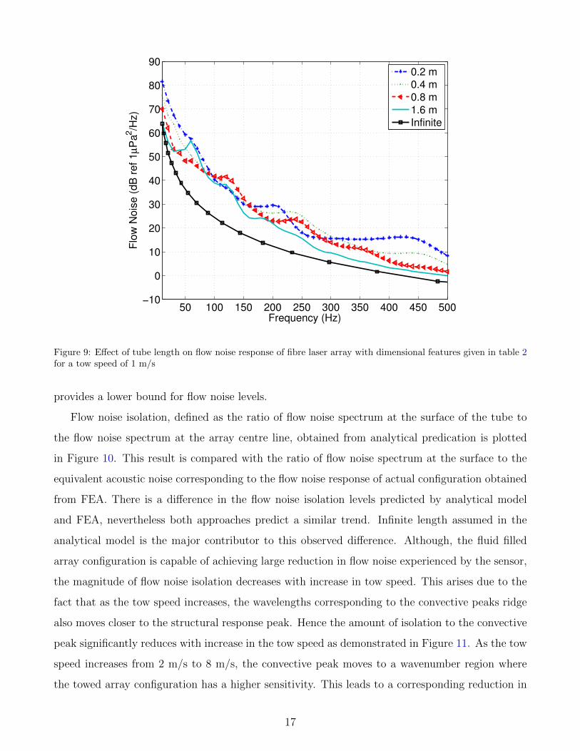
Finite element simulations were further extended to study the effect of tube length on the

flow noise spectrum. Length of the array section modelled in the analysis was varied from 0.2 m

to 1.6 m. Flow noise estimates were obtained for different tube lengths and they are compared

against analytical prediction for centre line pressure spectra using simplified geometry in Figure 9.

The wavenumber associated with breathing mode moves to lower wave numbers with increase in

the tube length. Hence flow noise response spectra marginally decreases with increase in the tube

length due to increased separation between the peaks in the excitation spectra and wavenumbers

associated with breathing modes. The maximum tube length considered in the analysis corresponds

to Nyquist spatial sampling rate for a maximum acoustic frequency of 500 Hz as thin-line arrays

for underwater surveillance applications rarely use adjacent sensor spacing greater than 1.5 meters

for linear arrays. The finite element results move closer to the analytical results with increase in

array section length. The effect of breathing modes associated with fluid filled array construction

reduces with increase in tube length since the breathing mode wavenumbers move further away

from the peaks in excitation spectrum. The analytical prediction using an infinite cylinder model

16

50 100 150 200 250 300 350 400 450 500−10

0

10

20

30

40

50

60

70

80

90

Frequency (Hz)

Flo

w N

ois

e (

dB

ref 1

µP

a2/H

z)

0.2 m

0.4 m

0.8 m

1.6 m

Infinite

Figure 9: Effect of tube length on flow noise response of fibre laser array with dimensional features given in table 2for a tow speed of 1 m/s

provides a lower bound for flow noise levels.

Flow noise isolation, defined as the ratio of flow noise spectrum at the surface of the tube to

the flow noise spectrum at the array centre line, obtained from analytical predication is plotted

in Figure 10. This result is compared with the ratio of flow noise spectrum at the surface to the

equivalent acoustic noise corresponding to the flow noise response of actual configuration obtained

from FEA. There is a difference in the flow noise isolation levels predicted by analytical model

and FEA, nevertheless both approaches predict a similar trend. Infinite length assumed in the

analytical model is the major contributor to this observed difference. Although, the fluid filled

array configuration is capable of achieving large reduction in flow noise experienced by the sensor,

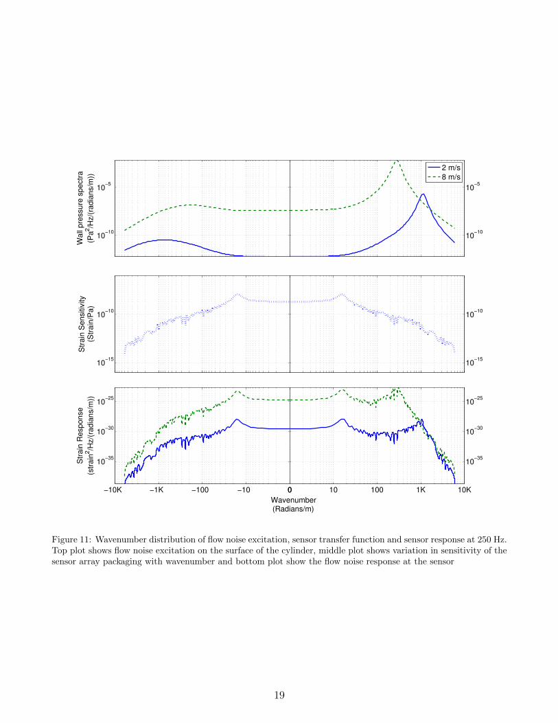
the magnitude of flow noise isolation decreases with increase in tow speed. This arises due to the

fact that as the tow speed increases, the wavelengths corresponding to the convective peaks ridge

also moves closer to the structural response peak. Hence the amount of isolation to the convective

peak significantly reduces with increase in the tow speed as demonstrated in Figure 11. As the tow

speed increases from 2 m/s to 8 m/s, the convective peak moves to a wavenumber region where

the towed array configuration has a higher sensitivity. This leads to a corresponding reduction in

17

1 2 3 4 5 6 7 830

35

40

45

50

55

60

65

70

75

80

Tow velocity (m/s)

Flo

w n

ois

e r

ed

uctio

n (

dB

)

100 Hz FEA

300 Hz FEA

500 Hz FEA

100 Hz Analytical

300 Hz Analytical

500 Hz Analytical

Figure 10: Variation in flow noise isolation with tow velocity

flow noise isolation.

5. Conclusion

The flow noise response of a diaphragm based fibre laser hydrophone array to wall pressure

fluctuations in an axisymmetric boundary layer at different tow speeds is presented. Equations for

the flow noise levels inside the array tube were obtained by modelling the towed array as an infinite

fluid filled tube submerged in water. Improved estimates of flow noise levels for the actual array

configuration were then obtained based on the finite element analysis of array sections. Though,

large reduction in flow noise levels can be achieved in fluid filled array configuration, the flow

noise isolation decreases with increase in tow speed. The flow noise arising due to turbulent wall

pressure fluctuations for the analysed configuration was found to be less than the usual ambient

noise levels in the sea for operating speeds below 2 m/s for frequencies greater than 200Hz. It was

also observed that the variation in flow noise levels with inter-hydrophone spacing is marginal for

the analysed configuration for typical sensor spacings used in thin-line towed arrays.

18

10−10

10−5

Wa

ll p

ressu

re s

pe

ctr

a

(Pa

2/H

z/(

rad

ian

s/m

))

10−10

10−5

2 m/s

8 m/s

10−15

10−10

Str

ain

Se

nsitiv

ity

(Str

ain

/Pa

)

10−15

10−10

0−10−100−1K−10K

10−35

10−30

10−25

Str

ain

Re

sp

on

se

(str

ain

2/H

z/(

rad

ian

s/m

))

Wavenumber(Radians/m)

0 10 100 1K 10K

10−35

10−30

10−25

Figure 11: Wavenumber distribution of flow noise excitation, sensor transfer function and sensor response at 250 Hz.Top plot shows flow noise excitation on the surface of the cylinder, middle plot shows variation in sensitivity of thesensor array packaging with wavenumber and bottom plot show the flow noise response at the sensor

19

References

Astley, R., Macaulay, G., Coyette, J., 1994. Mapped wave envelope elements for acoustical radia-

tion and scattering. Journal of Sound and Vibration 170, 97–118.

Batchellor, C.R., Edge, C., 1990. Some recent advances in fibre-optic sensors. Electronics &

Communication Engineering Journal 2, 175–184.

Bull, M., 1996. Wall-pressure fluctuations beneath turbulent boundary layers: some reflections on

forty years of research. Journal of Sound and Vibration 190, 299–315.

Carpenter, A., Kewley, D., 1983. Investigation of low wavenumber turbulent boundary layer pres-

sure fluctuations on long flexible cylinders, in: Eighth Australasian Fluid Mechanics Conference,

pp. 9A.1–9A.4.

Chase, D., 1980. Modeling the wavevector-frequency spectrum of turbulent boundary layer wall

pressure. Journal of Sound and Vibration 21, 29–67.

Chase, D., 1981. Further modeling of turbulent wall pressure on cylinder and its scaling

with diameter. Technical Report Technial Memo 21. DTIC. Http://www.dtic.mil/get-tr-

doc/pdf?AD=ADA113820.

Chase, D., 1987. The character of the turbulent wall pressure spectrum at subconvective wavenum-

bers and a suggested comprehensive model. Journal of Sound and Vibration 112, 125–147.

Ciappi, E., Magionesi, F., De Rosa, S., Franco, F., 2009. Hydrodynamic and hydroelastic analyses

of a plate excited by the turbulent boundary layer. Journal of Fluids and Structures 25, 321–342.

Cipolla, K., Keith, W., 2008. Measurements of the wall pressure spectra on a full-scale experimental

towed array. Ocean Engineering 35, 1052–1059.

Cipolla, K.M., Keith, W.L., 2003. Momentum thickness measurements for thick axisymmetric

turbulent boundary layers. Journal of Fluids Engineering 125, 569–575.

Corcos, G., 1967. The resolution of turbulent pressures at the wall of a boundary layer. Journal

of Sound and Vibration 6, 59–70.

Dahl, P.H., Miller, J.H., Cato, D.H., Andrew, R.K., 2007. Underwater ambient noise. Acoustics

Today 3, 23–33.

20

Dowling, A., 1998. Underwater flow noise. Theoretical and Computational Fluid Dynamics 10,

135–153.

Foley, A., Keith, W., Cipolla, K., 2011. Comparison of theoretical and experimental wall pres-

sure wavenumber–frequency spectra for axisymmetric and flat-plate turbulent boundary layers.

Ocean Engineering 38, 1123–1129.

Foster, S., Tikhomirov, A., van Velzen, J., Harrison, J., 2012. Recent advances in fibre optic array

technologies, in: Proceedings of Acoustics 2012, Fremantle, Australia, pp. 1–6.

Francis, S.H., Slazak, M., Berryman, J.G., 1984. Response of elastic cylinders to convective flow

noise - i. homogeneous, layered cylinders. Journal of the Acoustical Society of America 75,

166–172.

Franco, F., De Rosa, S., Ciappi, E., 2013. Numerical approximations on the predictive responses

of plates under stochastic and convective loads. Journal of Fluids and Structures 42, 296 – 312.

Graham, W., 1997. A comparison of models for the wavenumber–frequency spectrum of turbulent

boundary layer pressures. Journal of Sound and Vibration 206, 541–565.

Hill, D., Nash, P., Hawker, S., Bennion, I., 1998. Progress toward an ultra thin optical hydrophone

array, in: Proceedings of SPIE on European Workshop on Optical Fibre Sensors, Scotland, UK

pp.301–304.

Hill, D., Nash, P., Jackson, D., Webb, D., O’Neill, S., Bennion, I., Zhang, L., 1999. Fiber laser

hydrophone array, in: Proceedings of SPIE on Fiber Optic Sensor Technology and Applications,

Boston, USA. pp. 55–66.

Howe, M.S., 1998. Acoustics of fluid-structure interactions. Cambridge University Press, p. 208.

Kirkendall, C.K., Dandridge, A., 2004. Overview of high performance fibre-optic sensing. Journal

of Physics D: Applied Physics 37, R197–R216.

Knight, A., 1996. Flow noise calculations for extended hydrophones in fluid and solid filled towed

arrays. The Journal of the Acoustical Society of America 100, 245–251.

Ko, S.H., 1993. Performance of various shapes of hydrophones in the reduction of turbulent flow

noise. The Journal of the Acoustical Society of America 93, 1293–1299.

21

Ko, S.H., Nuttall, A.H., 1991. Analytical evaluation of flush-mounted hydrophone array response

to the corcos turbulent wall pressure spectrum. The Journal of the Acoustical Society of America

90, 579–588.

Kuttan Chandrika, U., Pallayil, V., Chitre, M., Kuselan, S., 2011. Estimated flow noise levels due

to a thin line digital towed array, in: Proceedings of OCEANS, 2011, Santander, Spain. pp. 1–4.

Kuttan Chandrika, U., Pallayil, V., Lim, K.M., Chew, C.H., 2013. Pressure compensated fibre

laser hydrophone: Modeling and experimentation. Journal of Acoustical Society of America 134,

2710–2718.

Leehey, P., 1988. Structural excitation by a turbulent boundary layer: an overview. Journal of

Vibration, Acoustics Stress and Reliability in Design 110, 220–225.

Pallayil, V., Muttuthupara, S., Chitre, M., Govind, K., 2009. Characterization of a digital thin line

towed array experimental assessment of vibration levels and tow shape, in: Underwater acoustic

measurements, pp. 21–26.

Skelton, E.A., James, J.H., 1997. Theoretical acoustics of underwater structures. Imperial College

Press London, pp. 241–250.

Snarski, S.R., Lueptow, R.M., 1995. Wall pressure and coherent structures in a turbulent boundary

layer on a cylinder in axial flow. Journal of Fluid Mechanics 286, 137–171.

Tutty, O.R., 2008. Flow along a long thin cylinder. Journal of Fluid Mechanics 602, 1–37.

22