Flow s imulations of generic vehicle model SAE type 4 and Open DrivAer ... · is DrivAer. DrivAer body was designed to have a similar exterior design feature to the existing production

Journal of Advanced Research in Fluid Mechanics and Thermal Sciences 37, Issue 1 (2017) 18-31

18

Journal of Advanced Research in Fluid

Mechanics and Thermal Sciences

Journal homepage: www.akademiabaru.com/arfmts.html

ISSN: 2289-7879

Flow simulations of generic vehicle model SAE type 4 and

DrivAer Fastback using OpenFOAM

Nur Haziqah Shaharuddin1,∗ , Mohamed Sukri Mat Ali1, Shuhaimi Mansor2, Sallehuddin Muhamad3, Sheikh

Ahmad Zaki Shaikh Salim1, Muhammad Usman4

1 Wind Engineering for Environment, Malaysia-Japan International Institute of Technology, Universiti Teknologi Malaysia, 54100 Kuala Lumpur,

Malaysia 2 Faculty of Mechanical Engineering, Universiti Teknologi Malaysia, 81310 Skudai, Johor, Malaysia 3 Razak School of Engineering and Advanced Technology, Universiti Teknologi Malaysia, 54100 Kuala Lumpur, Malaysia 4 Department of Mechanical Engineering, University Of Gujrat, Hayat Campus Jalalpur Road Gujrat, Pakistan

ARTICLE INFO ABSTRACT

Article history:

Received 23 August 2017

Received in revised form 22 September 2017

Accepted 6 October 2017

Available online 8 October 2017

The aim of this study is to simulate flow over two types of generic vehicle model. The

simulation is done using the open source CFD solver, OpenFOAM, which is based on

the finite volume method, where each of the control volume is treated for its flow

physical conservation using governing equations. The two different generic vehicle

models are SAE Type 4 (fullback) – strongly simplified model and DrivAer Fastback – a

more realistic vehicle model. Their flow structures are compared based on the CFD

results. The different in flow behaviours are shown clearly by each model due to the

geometry differences, where the SAE Type 4 is blunter, while the DrivAer Fastback is

more aerodynamic. Results showed that SAE Type 4 model able to produce large

turbulence wake structures and thus lead to higher value of drag coefficient compared

to the DrivAer Fastback model. The drag coefficient for the SAE Type 4 is 0.3722 and

the DrivAer Fastback is 0.2803.

Keywords:

OpenFOAM, Flow Simulation, SAE Type

4, DrivAer Fastback Copyright © 2017 PENERBIT AKADEMIA BARU - All rights reserved

1. Introduction

In this era, Computational Fluid Dynamics (CFD) together with the High Performance Computing

(HPC) Technology has given a great contribution to many industries [1, 6, 11, 12]. In the automotive

industry, CFD helps in accelerating the vehicle design process by reducing the relying on wind tunnel

experiments [1]. The computational resources necessary for the simulations have become more

affordable, and open source software is advance enough to handle the often complex geometries

that are commonly found in the automotive nowadays. Hence, it became one of the main design

tools for the external aerodynamic design for most vehicles development. It is difficult to obtain

detailed information of the flow field through experiments even though experiments are still

indispensable in modern vehicle aerodynamics as discussed by Angelina et al. [2]. In order to reduce

∗ Corresponding author.

E-mail address: [email protected] (Nur Haziqah Shaharuddin)

Penerbit

Akademia Baru

Open

Access

Journal of Advanced Research in Fluid Mechanics and Thermal Sciences

Volume 37, Issue 1 (2017) 18-31

19

Penerbit

Akademia Baru

the experiment cost, most of the designers would identify the flow behaviours through the

simulation in the early stage of the design before proceed with the experimental work.

The ability of the CFD simulation to capture the flow behaviour around a body is largely a function

of the predictive capability of the turbulence model. In this study, the turbulence modelling

evaluation is restricted to Reynolds Averaged Navier-Stokes (RANS) model, which assumes that the

entire spectrum of the turbulence can be approximated by a set of transport equations [3].

OpenFOAM (Open Source Field Operation and Manipulation), is an open source CFD solver that is

written in C++ toolbox for the development of customized numerical solvers, supplied with pre- and

post-processing utilities for the solution of continuum mechanics problems.

In recent year of research, general investigations of the flow field around a vehicle are strongly

focused on simplified car models, such as the Ahmed body [4] and the SAE model [5]. Both models

provide a better understanding in identifying and analysing the basic flow structures by reducing the

interference effects between different areas of vehicles. Previous works based on those simplified

models have provide a wide information on numerical and experimental that is suitable for the

validation purposes. However, they unable to reproduce important parts of the flow field involving

more complex flow phenomena such as the flow of a rotating wheels or interaction between car’s

underbody and road surfaces as studied by Angelina et al. [2].

2. Methodology

2.1 Problem Geometry

A simplified car model, SAE Type 4 (fullback) model is initially used in this study. Focused will be

given on this simple model as it provide a better understanding on the basic flow behaviour around

a vehicle before proceed to the investigation on a more complex vehicles models. Experimental and

numerical investigations that have been conducted by Hartmann et al. [6] used of the same model

to study the generation of wind noise produced by the flow from A-pillar and side view mirror of the

SAE Type 4 (fullback) model. They have used four different CFD codes for simulation which are

OpenFOAM, PowerFLOW, STAR-CD and STAR-CCM+. Validation process is done using experimental

results that have been generated in the Audi-wind tunnel. Their focus is given to the wind noise

generation and the results gave a very good agreement between the measured and simulated result

for all type of CFD solver used but slightly different in their flow visualisation. However, the basic

structure is captured correctly by all solvers.

Fig. 1. Dimension of simplified vehicle model SAE Type 4 [7]

Flow simulation is focused in this study in order to understand the basic flow structures around

a simplified car model, SAE Type 4 and the results are used to compare with a new realistic generic


Volume 37, Issue 1 (2017) 18-31

20

Penerbit

Akademia Baru

car model, DrivAer. The numerical simulations are done by using open source CFD solver,

OpenFOAM. Two different generic vehicle models are used in this study which is SAE Type 4 (Figure

1) and DrivAer Fastback (Figure 2). The SAE Type 4 model represents a simplified generic model while

DrivAer Fastback represents a more realistic generic car model.

SAE Type 4 (fullback) geometry and its dimension are identical to the model investigated by a

consortium of the German automotive manufacturers Audi, BMW, Daimler, Porsche and

Volkswagen. The height and width of the model are 1.20m and 1.60m respectively, while the length

is 2.45m. This simplified generic car model has no side mirror and hood.

The Institute of Aerodynamics and Fluid Mechanics of the Technical University of Munich (TUM),

in cooperation with Audi AG and the BMW Group have proposed a new realistic generic model, which

is DrivAer. DrivAer body was designed to have a similar exterior design feature to the existing

production cars and yet it would provide a more realistic result. The geometry is made available to

the public to access by the institute for individual study and therefore the fastback DrivAer geometry

is chosen for current study.

Fig. 2. Dimension of generic vehicle model DrivAer

Fastback [8]

The length of the DrivAer Fastback geometry provided is 4.61m, which is about two times longer

compared to the length of SAE Type 4 (fullback) geometry investigated.

2.2 Computational Domain

The computational domain for the flow simulation uses the pre-processing utilities available in

OpenFOAM. The simulations are performed using the SAE Type 4 (fullback) and DrivAer Fastback

model.

For a sufficient development of the turbulent characteristics of the flow, the distances between

the inlet, top and side of the computational domain from the models is located at 10D, where D =

(frontal area)1/2. The outlet is imposed at 20D downstream of the rear of the model to ensure the

outflow conditions do not affect the near-body wake and for allowing the wake to dissipate naturally.

The DrivAer Fastback model is made attached to the ground. Meanwhile the distance between the

ground and the bottom of the SAE Type 4 model is set at 0.2m in order to make the current study is

topologically similar to the real application used by production cars.


Volume 37, Issue 1 (2017) 18-31

21

Penerbit

Akademia Baru

Fig. 3. Computational domain for both SAE Type 4 and DrivAer Fastback model

The slip boundary condition is used at the upstream floor to prevent the development of

boundary layer, while no slip boundary condition is used at the downstream to allow the effect of

viscosity from the wake interacting with the downstream floor. In this study, only half model is

simulated to reduce the computational time.

The flow is assumed incompressible as the Mach number is below 0.01 and it is moving from the

inlet to the outlet of the domain with free stream velocity of 38.9m/s. Based on D = (frontal area)1/2,

the Reynolds number is Re = 3.59 x 106 for the SAE Type 4 model and Re = 4.16 x 106 for the DrivAer

Fastback model which make the flow is fully turbulent.

Fig. 4. Dimension of computational domain for both models (side view)


Volume 37, Issue 1 (2017) 18-31

22

Penerbit

Akademia Baru

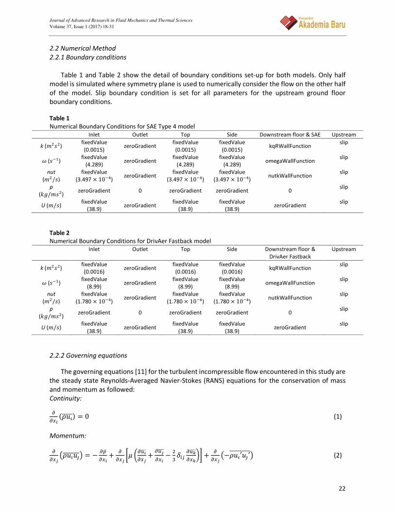
2.2 Numerical Method

2.2.1 Boundary conditions

Table 1 and Table 2 show the detail of boundary conditions set-up for both models. Only half

model is simulated where symmetry plane is used to numerically consider the flow on the other half

of the model. Slip boundary condition is set for all parameters for the upstream ground floor

boundary conditions.

Table 1

Numerical Boundary Conditions for SAE Type 4 model

Inlet Outlet Top Side Downstream floor & SAE Upstream

k (��) fixedValue

(0.0015) zeroGradient

fixedValue

(0.0015)

fixedValue

(0.0015) kqRWallFunction

slip

� (��) fixedValue


fixedValue

(4.289)

fixedValue

(4.289) omegaWallFunction

slip

nut

(��/�)

fixedValue

(3.497 × 10��) zeroGradient

fixedValue

(3.497 × 10��)

fixedValue

(3.497 × 10��) nutkWallFunction

slip

p

(� /��) zeroGradient 0 zeroGradient zeroGradient 0

slip

U (�/�) fixedValue

(38.9) zeroGradient

fixedValue

(38.9)

fixedValue

(38.9) zeroGradient

slip

Table 2

Numerical Boundary Conditions for DrivAer Fastback model

Inlet Outlet Top Side Downstream floor &

DrivAer Fastback

Upstream

k (��) fixedValue


fixedValue

(0.0016)

fixedValue

(0.0016) kqRWallFunction

slip

� (��) fixedValue

(8.99) zeroGradient

fixedValue

(8.99)

fixedValue

(8.99) omegaWallFunction

slip

nut

(��/�)

fixedValue

(1.780 × 10��) zeroGradient

fixedValue

(1.780 × 10��)

fixedValue

(1.780 × 10��) nutkWallFunction

slip

p

(� /��) zeroGradient 0 zeroGradient zeroGradient 0

slip

U (�/�) fixedValue

(38.9) zeroGradient

fixedValue

(38.9)

fixedValue

(38.9) zeroGradient

slip

2.2.2 Governing equations

The governing equations [11] for the turbulent incompressible flow encountered in this study are

the steady state Reynolds-Averaged Navier-Stokes (RANS) equations for the conservation of mass

and momentum as followed:

Continuity:

��

�� = 0 (1)

Momentum:

��

�� = − ��̅��

+ ��

! "�#$��

+ �#%��

− �& '()

�#*��*

+, + ��

�−��′��′�� (2)


Volume 37, Issue 1 (2017) 18-31

23

Penerbit

Akademia Baru

In equations (1) and (2), �̅ is mean density, .̅ is mean pressure, ! is the molecular viscosity and

−��′��′�� is the Reynold stress. The Reynold stress is solved using eddy-viscosity model based on the

Boussinesq assumption;

−��′��′�� = !/ "�#$��

+ �#%��

+ − �& 0�� + !/

�#*��*

1 '() (3)

where !/ the turbulent or eddy viscosity and k is the turbulent kinetic energy. For two-equation

turbulence models such as k-� and k-2 variants, the turbulent viscosity is computed through the

solution of two additional transport equations for the turbulent kinetic energy, and either the

turbulence dissipation rate, 2, or the specific dissipation rate, �. Shear Stress Transport (SST) k-� is

used in this study.

Some of the important computational settings are as followed:

Table 3

Solver setting used in OpenFOAM

Time stepping Steady State

Gradient Scheme 2nd order

Divergence Scheme Upwind (1st order)

Laplacian Scheme Linear (2nd order)

Interpolation Scheme Linear (2nd order)

Pressure Solver GAMG

Velocity Solver Gauss Seidel

Pressure-Velocity Coupling SIMPLE

No. of cells for SAE 1,101,047

No. of cells for DrivAer Fastback 1,596,854

2.3 Turbulence Model

2.3.1 Shear Stress Transport (SST) k-�

The SST k-� turbulence model provides robust and accurate formulation of the Standard k-�

model in the near-wall region, with the Standard k-2 in the far field. The SST k-� is more accurate

and reliable for a wider class of flows compared to the Standard k-ω, including adverse pressure

gradient flows.

However, variations exist in the production of � with comparison to the Standard k-� model.

The production of � is given by:

(4)

(5)

where is kinematic eddy viscosity and it is defined as;

(6)

In OpenFOAM the source or strain rate of the mean flow is defined as, , where

. The following closure coefficient is used in this study;

( )

∂

∂+

∂

∂+−=

∂

∂+

∂

∂

j

Tk

j

k

j

jx

k

xkP

x

kU

t

kνσνωβ *

( ) ( )iij

T

jj

jxx

kF

xxS

xU

t ∂

∂

∂

∂−+

∂

∂+

∂

∂+−=

∂

∂+

∂

∂ ω

ωσ

ωνσνβωα

ωωωω

112

21

22

Tν

( )21

1

,max SFa

kaT

ων =

22SS =2

2 ijSS =


Volume 37, Issue 1 (2017) 18-31

24

Penerbit

Akademia Baru

(7)

where y is the distance to the next surface,

(8)

(9)

(10)

(11)

where

(12)

(13)

(14)

3. Results and Discussions

3.1 Forces

Calculation for both drag and lift forces acting in the horizontal and vertical directions have been

done once the simulations have achieved the steady state. The coefficients reported for the

individuals cases are shown in Table 3 below. The coefficients are defined as:

34 = 56789:;8< (15)

3= = 5>789:;8< (16)

Table 3

Force coefficients for both models

Drag coefficients (mean) Lift coefficients (mean)

SAE Type 4 (fullback) 0.3722 -0.0774

DrivAer Fastback 0.2803 0.0447

By comparing both models, the SAE Type 4 model has a higher drag coefficient than the DrivAer

Fastback model. This is due to the geometry differences exists in both models, where DrivAer

Fastback model is more aerodynamic in shape compared to the SAE Type 4 model which is blunter.

Positive value in lift coefficient produced by DrivAer Fastback model might be due to the ground

effect [9]. The positive value indicates that vertical upwards acting force that bring about to lift the

car instead of remaining on the ground, that creates instability in car at high speed.

=

2

22

500,

*

2maxtanh

yy

kF

ν

ωβ

∂

∂= ωβτ k

x

UP

j

i

ijk *10,min

=

4

2

2

21

4,

500,

*

2maxmintanh

yCD

k

yy

kF

kω

σων

ωβ

∂

∂

∂

∂= −10

2 10,1

2maxii

kxx

kCD

ω

ωρσ ωω

( )1211 1 FF −+= φφφ

iii βαφ ,=

4403.0,9

521 == αα

10

9*,0828.0,

40

321 === βββ

85616.0,5.0,1.0,85034.02121

==== ωω αααα kk


Volume 37, Issue 1 (2017) 18-31

25

Penerbit

Akademia Baru

3.2 Flow Visualisations

3.2.1 p, U, Q and yPlus

Figure 3 shows the pressure distribution across the models. The front of the models stagnates air

and hence increases the pressure as presented by the red and yellow contour region and decreases

to negative values as it passes the top of the both models. At the inclined front windscreen of the

DrivAer Fastback model, the pressure increases due to the sudden angle difference between the

hood and windscreen.

Fig. 5. Pressure contours across SAE Type 4 (left) and DrivAer Fastback (right)

Fig. 6. Velocity flows over SAE Type 4 (fullback) model

Figure 5 and Figure 6 show the contour of velocity magnitude for SAE Type 4 and DrivAer Fastback

respectively. At the front regions of the both models, there is a low magnitude of velocity flow which

is between the ranges of 0 to 30 that indicates the velocity flow decreases as it is approaching the

model. For the SAE Type 4 (Figure 3.2), there are three layers of flow velocity magnitude observed at

the top of the model, where the lowest magnitude is created exactly on top of the model and it

increases to a free stream velocity as the flow velocity travels further away from the model. This

could be the effects from the simplified geometry of SAE Type 4 that creates a stagnation point

between the windscreen and the roof.


Volume 37, Issue 1 (2017) 18-31

26

Penerbit

Akademia Baru

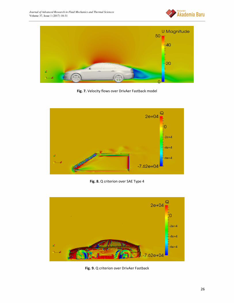
Fig. 7. Velocity flows over DrivAer Fastback model

Fig. 8. Q criterion over SAE Type 4

Fig. 9. Q criterion over DrivAer Fastback


Volume 37, Issue 1 (2017) 18-31

27

Penerbit

Akademia Baru

At the front of DrivAer Fastback hood, see Figure 7, the velocity flow increases due to the changes

in angle of geometry and reduces as it is approaching the gaps between the hood and windscreen.

The magnitude increases again when it passes over the top of the model and produces low pressure

level as shown on Figure 7. By comparing Figure 5 and Figure 6, both models are creating a low

magnitude of velocity flow at rear end of models. Larger size of velocity flow at the rear end is formed

by SAE Type 4. It shows that it produces larger wake compared to the DrivAer Fastback model.

Q-criterion for the SAE Type 4 and DrivAer Fastback are shown in Figure 8 and Figure 9

respectively. The value of Q produced by the DrivAer Fastback is larger than the SAE Type 4 because

there are more red regions are seen on the surface of DrivAer Fastback model where separations

occur at the mirror, the wheels and at rear end of the model. There are counter rotating vortices

found on the surface of DrivAer Fastback. For the SAE Type 4 the separations occur at the inclined

part and at the junction of the roof.

Fig. 10. Distribution of yPlus on the SAE Type 4 body

Fig. 11. Distribution of yPlus on the DrivAer Fastback body

Figure 10 and Figure 11 show the distribution of y+ on the SAE Type 4 and DrivAer Fastback model,

respectively. These y+ values are above the boundary layer log-law region. Figures show an obvious

of high values in y+ on the bottom and on the body of the models. There are only certain parts of the

body surfaces (mostly at front of the model), that having the values within the range of 0 to 300 and

this is due to the coarse mesh constructed away from the front region. To overcome this problem,

the distance of the first cell layer to the model surface should be located within the requirements of

y+ (30 < y+ < 300). Further refinement is required for these region in the future study.


Volume 37, Issue 1 (2017) 18-31

28

Penerbit

Akademia Baru

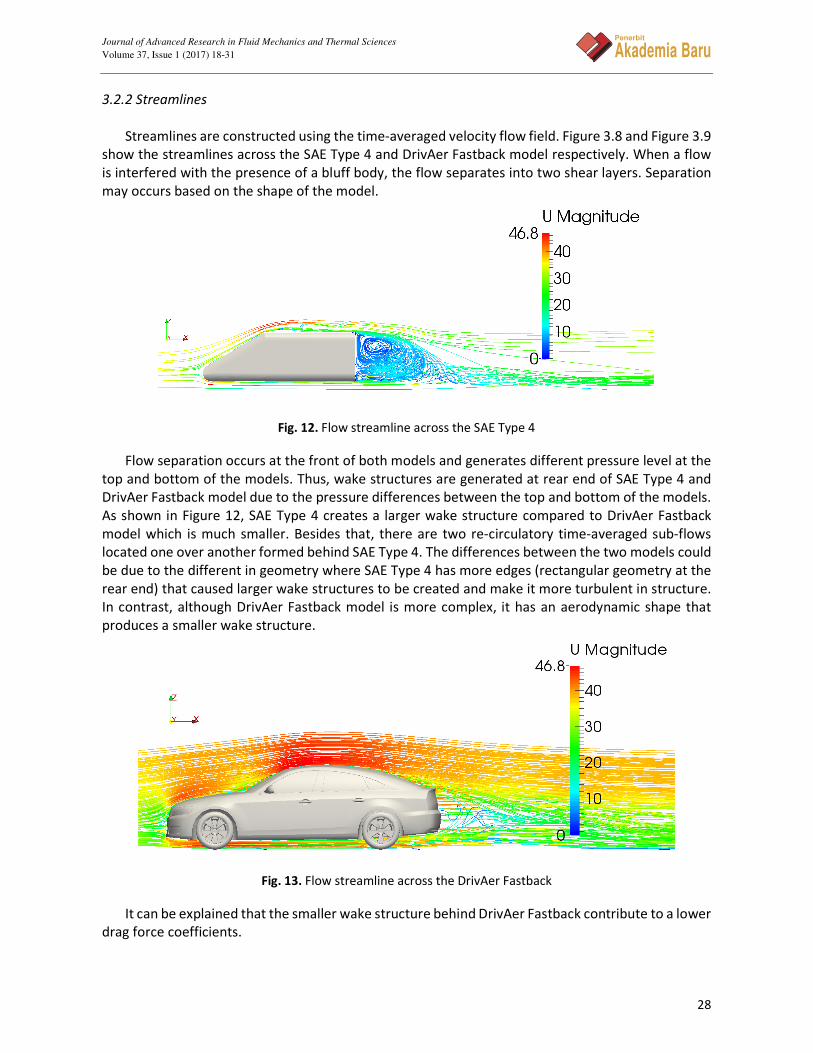
3.2.2 Streamlines

Streamlines are constructed using the time-averaged velocity flow field. Figure 3.8 and Figure 3.9

show the streamlines across the SAE Type 4 and DrivAer Fastback model respectively. When a flow

is interfered with the presence of a bluff body, the flow separates into two shear layers. Separation

may occurs based on the shape of the model.

Fig. 12. Flow streamline across the SAE Type 4

Flow separation occurs at the front of both models and generates different pressure level at the

top and bottom of the models. Thus, wake structures are generated at rear end of SAE Type 4 and

DrivAer Fastback model due to the pressure differences between the top and bottom of the models.

As shown in Figure 12, SAE Type 4 creates a larger wake structure compared to DrivAer Fastback

model which is much smaller. Besides that, there are two re-circulatory time-averaged sub-flows

located one over another formed behind SAE Type 4. The differences between the two models could

be due to the different in geometry where SAE Type 4 has more edges (rectangular geometry at the

rear end) that caused larger wake structures to be created and make it more turbulent in structure.

In contrast, although DrivAer Fastback model is more complex, it has an aerodynamic shape that

produces a smaller wake structure.

Fig. 13. Flow streamline across the DrivAer Fastback

It can be explained that the smaller wake structure behind DrivAer Fastback contribute to a lower

drag force coefficients.


Volume 37, Issue 1 (2017) 18-31

29

Penerbit

Akademia Baru

The flow behaviour at the wake region of SAE Type 4 and DrivAer Fastback are shown in Figure 14

and Figure 15.

Fig. 14. Velocity streamline at the back of the SAE Type 4

The velocity flows from the roof and side of the SAE Type 4 detached behind of the model and

formed a turbulence structure in the wake region. The shear layer coming off the end of model at

the sharp edges rolls up into a conical longitudinal vortex flow as shown in the blue region. This

phenomena is unseen at the wake region of DrivAer Fastback (see Figure 15) as it has a small

turbulence structure due to the flow is attached over the slant angle of model at the back.

Fig. 15. Velocity streamline at the back of DrivAer Fastback

The basic flow structure across the A-pillar over a simplified car model for the steady state result

is shown in Figure 16. The air flow from the windscreen separates at the A-pillar junction and

reattached with the flow on the roof. It then travels downstream and detached at the wake region

thus forming turbulence behaviour behind the SAE Type 4. More realistic behaviour can be studied

on the DrivAer Fastback model.


Volume 37, Issue 1 (2017) 18-31

30

Penerbit

Akademia Baru

Fig. 16. Velocity streamline at the front of the SAE Type 4

Fig. 17. Velocity streamline at the front of DrivAer Fastback

Figure 17 shows the streamline near the front pillar and side view mirror of DrivAer Fastback. The

flow travels from the front window separates in the front pillar and moves toward the roof side.

There are no large wake structures is observed behind the side view mirror as this study is done under

the steady state condition. However, there are flow separations at the front pillar and side view

mirror that interfere each other and attached together with the wake formed behind.


Volume 37, Issue 1 (2017) 18-31

31

Penerbit

Akademia Baru

4. Conclusion

Based on the analysis performed, it can be concluded that the CFD flow simulation results

produced for the simplified vehicle SAE Type 4 model is slightly different to the realistic vehicle

DrivAer Fastback model under the steady state performance. The basic understanding on the flow

structures over a generic vehicle model has been studied. The different in turbulence structure

formed at the wake region of each model has proved that the flow behaviours of a body are strongly

related to its geometry and thus affecting the drag and lift force acting on the body at once.

References [1] Shinde, G., Joshi, A. and Kishor, N. “Numerical Investigations of the DrivAer Car Model Using Opensource CFD

Solver OpenFOAM.” Tata Consultancy Services, Pune, India.

[2] Heft, Angelina I., Thomas Indinger, and Nikolaus Adams. "Experimental and numerical investigation of the DrivAer

model." In Rio Grande, Puerto Rico: ASME 2012 Fluids Engineering Summer Meeting. 2012.

[3] Ashton, N., and A. Revell. "Investigation into the predictive capability of advanced Reynolds-Averaged Navier-

Stokes models for the DrivAer automotive model." In The International Vehicle Aerodynamics Conference, p. 125.

Woodhead Publishing, 2014.

[4] Ahmed, Syed R., G. Ramm, and G. Faltin. Some salient features of the time-averaged ground vehicle wake. No.

840300. SAE Technical Paper, 1984.

[5] Cogotti, Antonello. A parametric study on the ground effect of a simplified car model. No. 980031. SAE Technical

Paper, 1998.

[6] Hartmann, Michael, Joerg Ocker, Timo Lemke, Alexandra Mutzke, Volker Schwarz, Hironori Tokuno, Reinier

Toppinga, Peter Unterlechner, and Gerhard Wickern. "Wind Noise Caused by the Side-Mirror and A-Pillar of a

Generic Vehicle Model." In 18th AIAA/CEAS Aeroacoustics Conference (33rd AIAA Aeroacoustics Conference), p.

2205. 2012.

[7] Islam, Moni, Friedhelm Decker, Michael Hartmann, Anke Jaeger, Timo Lemke, Joerg Ocker, Volker Schwarz, Frank

Ullrich, Andreas Schröder, and André Heider. "Investigations of sunroof buffeting in an idealised generic vehicle

model-part I: Experimental results." AIAA Paper 2900 (2008): 2008.

[8] Heft, Angelina I., Thomas Indinger, and Nikolaus A. Adams. Introduction of a new realistic generic car model for

aerodynamic investigations. No. 2012-01-0168. SAE Technical Paper, 2012.

[9] Ahmed, H., and S. Chacko. "Computational optimization of vehicle aerodynamics." In Proc. of the 23rd

International DAAM Symposium, vol. 23, no. 1, pp. 313-318. 2012.

[10] Nouzawa, Takahide, Ye Li, Naohiko Kasaki, and Takaki Nakamura. "Mechanism of aerodynamic noise generated

from front-pillar and door mirror of automobile." Journal of Environment and Engineering 6, no. 3 (2011): 615-

626.

[11] Tey, W. Y., Yutaka, A., Sidik, N. A. C., and Goh, R. Z. “Governing Equations in Computational Fluid Dynamics:

Derivations and a Recent Review.” Journal of Progress in Energy and Environment 1, no. 1 (2017): 1-19.

[12] Too, J. H. Y., and C. S. N. Azwadi. "Numerical Analysis for Optimizing Solar Updraft Tower Design Using

Computational Fluid Dynamics (CFD)." J. Adv. Res. Fluid Mech. Therm. Sci. 22 (2016): 8-36.

Documents

Flow s imulations of generic vehicle model SAE type 4 and Open DrivAer ... · is DrivAer. DrivAer body was designed to have a similar exterior design feature to the existing production