Flow Sensing for Height Estimation and Control of a Rotor in Ground Effect:Modeling and Experimental Results

Chin Gian Hooichingian.hooi@umd.edu

Graduate Research Assistant

Francis D. Lagorflagor@umd.edu

Graduate Research Assistant

Derek A. Paleydpaley@umd.edu

Willis H. Young Jr. Associate ProfessorDepartment of Aerospace Engineering and Institute for Systems Research

University of Maryland, College Park, MD, USA

ABSTRACTThis paper describes a dynamic controller for rotorcraft landing and hovering in ground effect using feedback con-trol based on flowfield estimation. The rotor downwash in ground effect is represented using a ring-source potentialflow model selected for real-time use. Experimental verification of the flow model is also presented. A nonlineardynamic model of the rotorcraft in ground effect is presented with open-loop analysis and closed-loop control simu-lation. Experimental results of the open-loop dynamics are presented and the effect of motor dynamics on the overalldynamics are investigated. Flowfield velocity measurements are assimilated into a grid-based recursive Bayesian filterto estimate height above ground in both simulation and experiment. Height tracking in ground effect and landing areimplemented with a dynamic linear controller. Experimental validation of the closed-loop controller is ongoing.

INTRODUCTION

Rotorcraft operation in ground effect (IGE) presents substan-tial challenges for vehicle control, including landing with low-impact velocity and maintaining near-ground hover in low-visibility conditions such as brownout (Ref. 1), fog (Ref. 2),snow or darkness. Safe operation IGE requires a controllercapable of handling uncertainty. Previous authors have de-veloped landing controllers based on robust or adaptive con-trol techniques. For example, Serra and Cunha (Ref. 3) adoptan affine parameter-dependent model that describes the he-licopter linearized error dynamics for a predefined landingregion and implements H2 feedback control. Mahony andHamel (Ref. 4) develop a parametric adaptive controller thatestimates the helicopter aerodynamics onboard and modulatesthe motor torque, rather than the collective pitch, during take-off and landing and takes advantage of the reduced sensitiv-ity of the control input to aerodynamics effects. Nonaka andSugizaki (Ref. 5) implement ground-effect compensation andintegral sliding mode control to suppress the modeling errorof the vehicle dynamics in ground effect. These control tech-niques often require a system model with empirically fit aero-dynamic coefficients that are unique to each vehicle.

Safe operation IGE also requires accurate estimation ofthe proximity and relative orientation of the ground plane.Height-estimation methods currently exist for micro aerial ve-hicles (MAVs) based on ultrasonic, barometric pressure or op-tical sensors. However, ultrasonic sensors work only for prox-imity sensing and do not work well for an angled or irregularground plane (Ref. 6). Barometric pressure sensors typically

Presented at the AHS 71st Annual Forum, Virginia Beach,Virginia, May 5–7, 2015. Copyright c© 2015 by the AmericanHelicopter Society International, Inc. All rights reserved.

work well for large height differentials (Ref. 7), but are sen-sitive to fluctuations in atmospheric pressure, which results insensor drift. Likewise, the effectiveness of vision-based sen-sors is limited in degraded visual environments. This paperdevelops a hover and landing controller that uses rotor down-wash flow-velocity measurements and an aerodynamic modelto estimate the height above ground, thereby providing an ad-ditional sensing modality for hovering and landing IGE.

Previous authors have quantified ground effect empiricallyor through the use of an underlying aerodynamic model. Non-aka and Sugizaki (Ref. 5) take an empirical approach to mea-suring the ground effect on rotor thrust as a function of mo-tor voltage. Mahony and Hamel (Ref. 4) use an approxima-tion of the down-flow velocity ratio based on a piecewise lin-ear approximation of Prouty (Ref. 8) to estimate rotor-thrustvariation IGE. Higher fidelity analytical models include pre-scribed wake vortex modeling (Ref. 9) and free vortex mod-eling (Ref. 10), which seek to accurately predict the natureof the rotor wake vortices. Cheeseman and Bennett (Ref. 11)provide a classic analytical model for ground effect, which weadopt for this work, based on aerodynamic modeling usingthe method of images. The use of an aerodynamic model per-mits comparison to measurements from sensors such as multi-component differential-pressure airspeed sensors (Ref. 12).Lagor et al. (Ref. 13) and DeVries et al. (Ref. 14) have previ-ously shown that a reduced-order flow model can be rapidlyevaluated within a Bayesian filter to perform estimation andcontrol tasks in an uncertain flow environment.

Our previous paper (Ref. 15) developed a dynamic con-troller for hover and landing IGE based on a flow modelfor height estimation. Rotorcraft downwash IGE was mod-eled using potential flow theory. We extended the model ofCheeseman and Bennett (Ref. 11) using multiple ring sources;

1

the mirror images create a ground plane. The reduced-ordermodel relates the flowfield velocities to height IGE; it is capa-ble of relatively fast evaluation for control purposes. A nonlin-ear dynamic model of rotorcraft landing IGE was presented,assuming a rigid rotor commonly found in MAV rotorcraft(Ref. 16). Height estimation of rotorcraft IGE using spatiallydistributed airspeed measurements was accomplished with agrid-based recursive Bayesian filter. The Bayesian frameworkis capable of fusing data from additional sensing modalitiesand for estimation of additional states, such as roll and pitchrelative to the landing platform. The feedback controller wasimplemented in simulation to illustrate the theoretical results.

This paper expands on our previous paper by including ex-perimental verification of parts of the flow modeling, sensingand control framework. The contributions of this paper are (1)an improved ring-source potential flow model consistent withexperimental observations; (2) a nonlinear dynamics modelof a compound pendulum heave test stand; (3) experimen-tal verification of our ring-source potential flow model andheight estimation framework; and (4) experimental results ofthe open-loop compound pendulum dynamics.

Flow Estimation and Closed-Loop Control System Archi-tecture

The control and estimation architecture developed and simu-lated in this paper is shown in Fig. 1. The flow velocities vand w, in the radial and vertical axes, respectively, are sim-ulated using the ring-source potential flow model. The ro-torcraft dynamics are simulated using a nonlinear state-spacemodel. Flow measurements v and w are presumed to be cor-rupted with additive sensor noise. These flow measurementsare used by a grid-based recursive Bayesian filter to estimaterotorcraft height and a feedback controller seeks to drive thevehicle to the commanded height.

Fig. 1. Block diagram for closed-loop flow sensing and con-trol.

Experimental Instrumentation Architecture

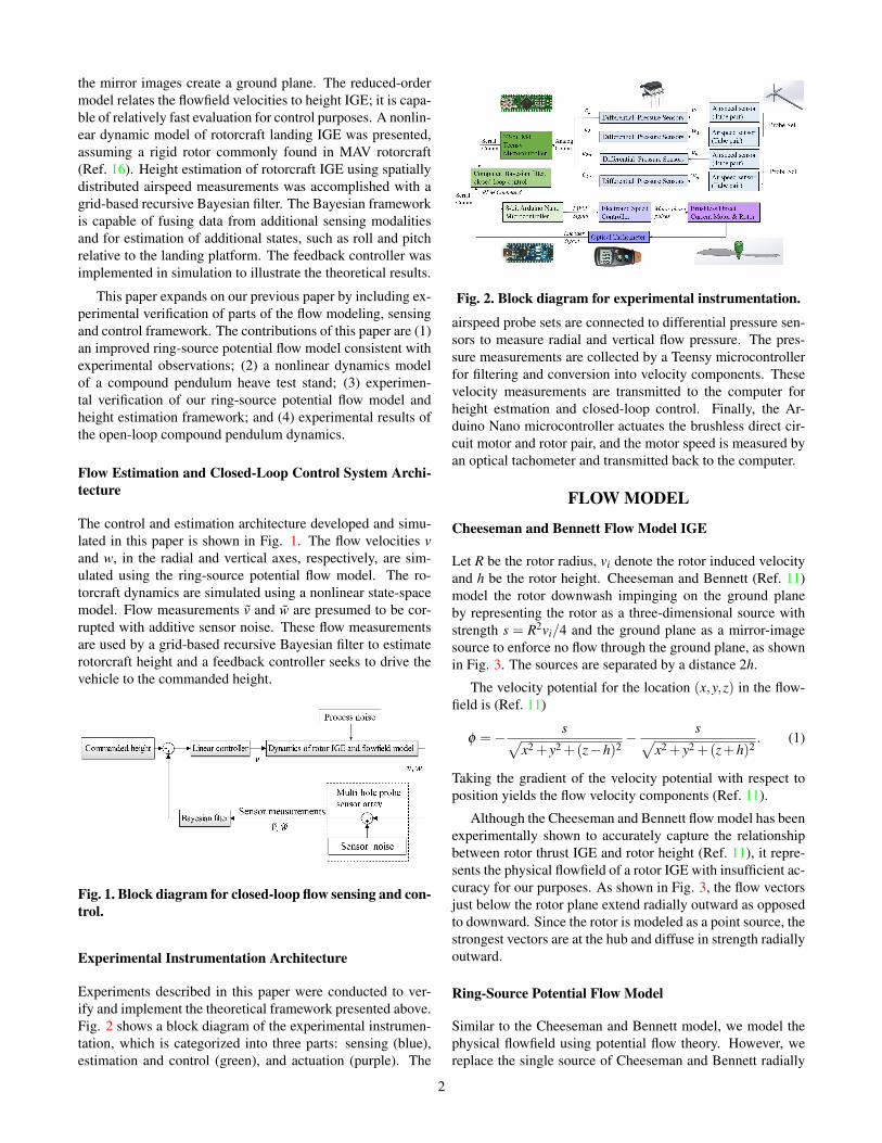
Experiments described in this paper were conducted to ver-ify and implement the theoretical framework presented above.Fig. 2 shows a block diagram of the experimental instrumen-tation, which is categorized into three parts: sensing (blue),estimation and control (green), and actuation (purple). The

Fig. 2. Block diagram for experimental instrumentation.

airspeed probe sets are connected to differential pressure sen-sors to measure radial and vertical flow pressure. The pres-sure measurements are collected by a Teensy microcontrollerfor filtering and conversion into velocity components. Thesevelocity measurements are transmitted to the computer forheight estmation and closed-loop control. Finally, the Ar-duino Nano microcontroller actuates the brushless direct cir-cuit motor and rotor pair, and the motor speed is measured byan optical tachometer and transmitted back to the computer.

FLOW MODEL

Cheeseman and Bennett Flow Model IGE

Let R be the rotor radius, vi denote the rotor induced velocityand h be the rotor height. Cheeseman and Bennett (Ref. 11)model the rotor downwash impinging on the ground planeby representing the rotor as a three-dimensional source withstrength s = R2vi/4 and the ground plane as a mirror-imagesource to enforce no flow through the ground plane, as shownin Fig. 3. The sources are separated by a distance 2h.

The velocity potential for the location (x,y,z) in the flow-field is (Ref. 11)

φ =− s√x2 + y2 +(z−h)2

− s√x2 + y2 +(z+h)2

. (1)

Taking the gradient of the velocity potential with respect toposition yields the flow velocity components (Ref. 11).

Although the Cheeseman and Bennett flow model has beenexperimentally shown to accurately capture the relationshipbetween rotor thrust IGE and rotor height (Ref. 11), it repre-sents the physical flowfield of a rotor IGE with insufficient ac-curacy for our purposes. As shown in Fig. 3, the flow vectorsjust below the rotor plane extend radially outward as opposedto downward. Since the rotor is modeled as a point source, thestrongest vectors are at the hub and diffuse in strength radiallyoutward.

Ring-Source Potential Flow Model

Similar to the Cheeseman and Bennett model, we model thephysical flowfield using potential flow theory. However, wereplace the single source of Cheeseman and Bennett radially

2

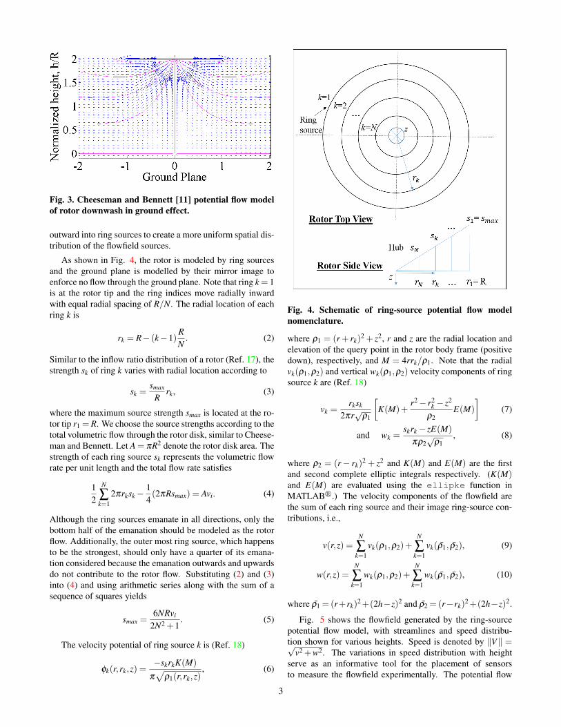
Fig. 3. Cheeseman and Bennett [11] potential flow modelof rotor downwash in ground effect.

outward into ring sources to create a more uniform spatial dis-tribution of the flowfield sources.

As shown in Fig. 4, the rotor is modeled by ring sourcesand the ground plane is modelled by their mirror image toenforce no flow through the ground plane. Note that ring k = 1is at the rotor tip and the ring indices move radially inwardwith equal radial spacing of R/N. The radial location of eachring k is

rk = R− (k−1)RN

. (2)

Similar to the inflow ratio distribution of a rotor (Ref. 17), thestrength sk of ring k varies with radial location according to

sk =smax

Rrk, (3)

where the maximum source strength smax is located at the ro-tor tip r1 =R. We choose the source strengths according to thetotal volumetric flow through the rotor disk, similar to Cheese-man and Bennett. Let A = πR2 denote the rotor disk area. Thestrength of each ring source sk represents the volumetric flowrate per unit length and the total flow rate satisfies

12

N

∑k=1

2πrksk−14(2πRsmax) = Avi. (4)

Although the ring sources emanate in all directions, only thebottom half of the emanation should be modeled as the rotorflow. Additionally, the outer most ring source, which happensto be the strongest, should only have a quarter of its emana-tion considered because the emanation outwards and upwardsdo not contribute to the rotor flow. Substituting (2) and (3)into (4) and using arithmetic series along with the sum of asequence of squares yields

smax =6NRvi

2N2 +1. (5)

The velocity potential of ring source k is (Ref. 18)

φk(r,rk,z) =−skrkK(M)

π√

ρ1(r,rk,z), (6)

Fig. 4. Schematic of ring-source potential flow modelnomenclature.

where ρ1 = (r+ rk)2 + z2, r and z are the radial location and

elevation of the query point in the rotor body frame (positivedown), respectively, and M = 4rrk/ρ1. Note that the radialvk(ρ1,ρ2) and vertical wk(ρ1,ρ2) velocity components of ringsource k are (Ref. 18)

vk =rksk

2πr√

ρ1

[K(M)+

r2− r2k − z2

ρ2E(M)

](7)

and wk =skrk− zE(M)

πρ2√

ρ1, (8)

where ρ2 = (r− rk)2 + z2 and K(M) and E(M) are the first

and second complete elliptic integrals respectively. (K(M)and E(M) are evaluated using the ellipke function inMATLABr.) The velocity components of the flowfield arethe sum of each ring source and their image ring-source con-tributions, i.e.,

v(r,z) =N

∑k=1

vk(ρ1,ρ2)+N

∑k=1

vk(ρ1, ρ2), (9)

w(r,z) =N

∑k=1

wk(ρ1,ρ2)+N

∑k=1

wk(ρ1, ρ2), (10)

where ρ1 =(r+rk)2+(2h−z)2 and ρ2 =(r−rk)

2+(2h−z)2.

Fig. 5 shows the flowfield generated by the ring-sourcepotential flow model, with streamlines and speed distribu-tion shown for various heights. Speed is denoted by ‖V‖ =√

v2 +w2. The variations in speed distribution with heightserve as an informative tool for the placement of sensorsto measure the flowfield experimentally. The potential flow

3

Fig. 5. Flowfield of ring-source potential flow model evaluated at various heights, depicting streamlines and speed dis-tributions, where speed ‖V‖=

√v2 +w2.

model is qualitatively similar to the flow visualization modelof the flow below a rotor IGE by Lee et al. (Ref. 19).

Moving from the rotor plane to the ground close to therotor hub, the flow decelerates and forms a stagnation re-gion. The flow deceleration region is easiest to distinguish forh=1.0R in Fig. 5. In contrast, the flow acceleration region iswhere the streamlines change direction from pointing down-ward to pointing radially outward. As the rotor approachesthe ground, the streamlines are compressed, which is best il-lustrated for h=0.5R in Fig. 5. Evidently, the flow speed isthe highest in the flow acceleration region for the h=0.5R caseas opposed to the h=2.0R case, since the flow is being com-pressed more with less space between the rotor plane and theground. This effect is analogous to moving a water jet (therotor) closer to a wall (the ground plane), since the jet speedin the flow acceleration region is highest when it is close tothe wall.

Although the rotor downwash IGE as visualized in thework of Lee et al. (Ref. 19) is not laminar, we model it us-ing potential flow theory and account for turbulence with pro-cess noise (see Height and Speed Estimation Section). Wemodel the mean velocity of the dominant flow and treat the

turbulence and other secondary effects, such as blade tip vor-tices, as fluctuations away from the mean. Flow velocity com-ponent measurements V are collected below the rotor in theexperimental setup. Airspeed measurements of the sort de-scribed in (Ref. 12) contain two flow velocity components,radial v and vertical w, at each airspeed probe set location andare collected in an array configuration to sample the flowfieldat multiple spatial locations. Measurement V corresponds toeither the radial v or the vertical w velocity component. Weassume V is corrupted by zero-mean Gaussian white noise η

with standard deviation ση and zero mean, resulting in themeasurement model

V =V +η . (11)

DYNAMICS AND CONTROL

Dynamics of Rotorcraft Operation IGE

Fig. 6 shows the free-body diagram of a rotorcraft in whichthe tailrotor counter torque is not shown. Applying Newton’ssecond law in the ez direction yields

mh = TIGE −mg−b1h, (12)

4

Fig. 6. Free-body diagram of rotorcraft in ground effect.

where TIGE is the rotor thrust IGE, m is the mass of the rotor,h and h are the vertical velocity and acceleration respectively,g is the gravitational acceleration and b1 is the damping co-efficient due to aerodynamics or another source. Modelingthe rotor thrust T as a function of rotor rotational speed ω

yields (Ref. 16)

T = kω2. (13)

The rotor thrust is augmented for ground effect using theCheeseman and Bennett model, which captures the essentialcharacteristic of the relationship between thrust and heightIGE, i.e.,

TIGE =1

1− R2

16h2

T =16h2

16h2−R2 T . (14)

Based on experimental data, Leishman (Ref. 17) suggests thatmodel (14) is valid for 2.0 ≥ h/R ≥0.5. It is assumed hence-forth that the rotorcraft has landed when h/R =0.5, which isreasonable since the rotor distance above the landing gear istypically greater than 0.5R. Thrust IGE (14) is substituted into(12) to obtain the dynamics of a rotorcraft IGE,

h =16h2kω2

(16h2−R2)m−g−b1h. (15)

Linear State Space Form

The state vector Z ∈ R2 is defined as

Z =

[hh

]=

[z1z2

], (16)

where h is the landing speed. Since the rotor rotational speedis regulated, we define ν = kω2/m as the control input. Thenonlinear state space form is

Z =

[hh

]=

[z2

16z21

16z21−R2 ν−g

]. (17)

An equilibrium control input ν∗ is necessary to keep the ro-torcraft hovering at a corresponding equilibrium height z∗1 (orto land safely). Solving (17) for the equilibrium condition,Z∗ = 0, the equilibrium control input is

ν∗ = g

16z∗21 −R2

16z∗21. (18)

Fig. 7. Open-loop dynamics of rotorcraft in ground effectwith constant input ν = ν∗. Initial conditions for heightand speed are (1.5m, 0.25m/s).

Fig. 7 depicts the simulation results of the open-loop nonlin-ear dynamics for initial height and speed (1.5m and 0.25m/s)and constant input ν = ν∗.In order to implement a linear controller for the nonlinear dy-namics (17), the Jacobian matrices are needed. The Jacobians

A =

[0 1

−2gR2

z∗1(16z∗21 −R2)0

]and B =

[0

16z∗2116z∗21 −R2

](19)

are the partial derivatives of the right-hand side of (17) withrespect to Z and ν , respectively. The linear system dynamicsare

Z = AZ +Bν . (20)

Nonlinear Dynamics with Linear Observer-based Feed-back Control

The state space system (17) in control affine form is

Z = f (Z)+g(Z)ν , (21)

where

f (Z) =[

z2−g

]and g(Z) =

[0

16z21

16z21−R2

]. (22)

Fig. 7 shows that the constant-input open-loop nonlinear sys-tem with ν = ν∗ oscillates about the equilibirum point, whichimplies that feedback control is needed to asymptotically sta-bilize z1 to the desired height. A linear controller to be usedwith the nonlinear system dynamics is

ν = ν∗+∆ν , (23)

5

Fig. 8. Closed-loop dynamics of rotorcraft in ground effectwith full-state feedback, Z = Z using the linear controller(23).

where ∆ν = −K(Z − Z∗), K = [K1 K2] and Z =[z1 z2]

T denotes the estimated states. The closed-loop dy-namics with the linear output-feedback controller (23) are

Z =

[z2−g

]+

[0

16z21

16z21−R2

](ν∗+∆ν), (24)

i.e.,

Z=

[z2

−g+ 16z21

16z21−R2

(g 16z∗21 −R2

16z∗21−K1(z1− z∗1)−K2z2

)]. (25)

Figure 8 compares the nonlinear closed-loop dynamics(25) to the linear closed-loop dynamics (20), using linear con-troller (23). The simulation is implemented using full-statefeedback, Z = Z. The optimal gains K are provided by LinearQuadratic Regulator (LQR) and the Jacobian matrices in (19)are evaluated at the equlibrium height. Initial conditions forthe height and speed are (1.8m, 0.9m/s) and desired steady-state conditions are (0.75m, 0m/s).

Dynamics of Compound Pendulum Heave Test Stand

Our experimental setup was constructed as a compound pen-dulum with one degree of freedom in the heave direction asshown in Fig. 9. This setup allows the use of journal bear-ings, which are smoother than linear carriages and rails in avertical setup. This setup also has the added benefit of allow-ing a counterweight to balance the system weight and to re-duce the motor load. Figure 10 shows the free-body diagramof the compound pendulum. The lateral (ey) displacement canbe minimized by mounting the setup at the midstroke, i.e., ata height of 1.25R.

The angular momentum of the compound pendulum is

ho = Ioθex, (26)

where Io is the moment of inertia about point O, θ is the posi-tive clockwise angle from vertical and θ is the angular veloc-ity of the pendulum. The time derivative of the angular mo-mentum equals the moment about point O. In the ex direction,

Fig. 9. Compound pendulum heave test stand.

Fig. 10. Free body diagram of compound pendulum heavetest stand.we have

Ioθ = LTIGE sinθ − l1gsinθ(m+M1)+ l2M2gsinθ −b2θ , (27)

where θ is the angular acceleration; l1, l2 and L are the dis-tances from O to the center of mass, O to counterweight M2and O to rotor mass m respectively; M1 is the mass of the pen-dulum setup and b2 is the damping coefficient due to aerody-namics and/ or friction. In terms of the height h= L2−Lcosθ ,we have

h = Lθ sinθ , (28)h = Lθ

2 cosθ +Lθ sinθ . (29)

Since the compound pendulum is mounted at midstroke,we approximate θ ≈ π/2, which implies

h≈ L2, h≈ Lθ and h≈ Lθ . (30)

Likewise, the moment of inertia Io is

Io = mL2 +13

M1(L+ l2)2 +M2l22. (31)

6

Substituting (14) and (30) into (27) yields the dynamics of thecompound pendulum heave test stand,

h =1Io

[16h2kω2L2

(16h2−R2)− l1Lg(m+M1)+ l2LgM2

]−bh, (32)

where b = b2/Io. Note that as the mass of the compound pen-dulum setup M1 and the counterweight M2 go to zero, thecompound pendulum dynamics (32) reduce to the rotorcraftIGE dynamics (15).

HEIGHT AND SPEED ESTIMATION

The Bayesian filter (Ref. 14) (Ref. 20) is a probabilistic ap-proach for estimation that assimilates noisy measurementsinto a probability density function (PDF) using nonlinearsystem dynamics and observation operators. (The optimalBayesian filter for linear systems with linear measurementsand Gaussian noise is the Kalman filter (Ref. 21), whereas acommon Bayesian filter for nonlinear systems with nonlinearobservation and noise models is the particle filter (Ref. 22).)A grid-based recursive Bayesian filter can be rapidly imple-mented for a low-dimensional state-space representation ofthe rotorcraft downwash with linear parameter estimates and anonlinear measurement model.1 It is of note that even thoughlinear paramater estimates and Gaussian white noise is as-sumed for our measurement and process noise, these are notrequired assumptions for the Bayesian filter.

Estimation Step

The Bayesian framework consists of the estimation and theprediction step. In the estimation step, the Bayesian filter inthe form of (Ref. 14) estimates the vehicle height based on theflow-velocity measurements from an array of differential pres-sure sensors. Grid-based Bayesian estimation is performedrecursively, in which the finite parameter space over heighth is discretized and the PDFs are evaluated on this grid foreach new measurement. Let h be the single state of a one-dimensional Bayesian filter. Recall that the noisy flow mea-surement V is corrupted with zero mean Gaussian noise as in(11). Let L = {V1, ...,Vm} denote the set of observations fromm sensors. Note that each velocity component measurement(even at the same location) is treated as a separate measure-ment. The posterior probability of the state h given the mea-surements L is (Ref. 14)

P(h|L) = cP(L|h)P(h|L0), (33)

where c is the scaling factor chosen so that P(h|L) has unitintegral over the state space. The likelihood function P(L|h)

1As an alternative, the Unscented Kalman filter (Ref. 23) isan approximate nonlinear estimator that differs the inevitabledivergence with highly nonlinear systems or measurements(Ref. 21). The particle filter (Ref. 22) provides high perfor-mance estimation but requires careful selection of its estima-tion state vector because it is prone to sample impoverishmentand requires careful tuning.

is the conditional probability of the observations L given thestate h and P(h|L0) represents the prior probability distribu-tion. During initialization or in the absence of measurements,the prior probability P(h|L0) is uniform.

We choose a Gaussian likelihood function for the measure-ments Vl , l = 1, ...,m, i.e.,

P(Vl |h) =1√

2πσexp[− 1

2σ2 (Vl−Vl)2]

, (34)

where Vl is the flow at height h generated from the flow model(9) or (10) and σ2 is the measurement variance. The posteriorprobability density of the state h is obtained using the jointmeasurement likelihood combining the measurements takenfrom all m sensors (Ref. 14), i.e.,

P(h|L) = c

(m

∏l=1

P(Vl |h)

)P(h|L0). (35)

The estimated height h corresponding to the mode (supre-mum) of the posterior probability P(h|L) provides the max-imum likelihood estimate of the flowfield parameters.

Spatial integration over the sensor array is accomplishedby (35), whereas temporal integration is accomplished by as-signing the posterior of the current time step to be the priorfor the next time step.

Prediction Step

The prediction step consists of shifting and diffusing the prob-ability mass to account for the vehicle dynamics using theChapman-Kolmogorov equation (Ref. 22),

P(h(t +∆t)|L(t))

=∫

P(h(t +∆t)|h(t))P(h(t)|L(t))dh(t), (36)

where t is the current time step and ∆t is the time step interval.Numerically, the probability density is shifted along the gridaccording to the estimated speed z2. If the estimated speed z2is positive, we shift the PDF to the right and vice-versa. Thenumber of grid points to shift is determined by the product ofthe estimated speed z2 and time interval. After shifting, theprobability density is normalized to ensure the PDF integratesto one.

To account for uncertainty in the motion model, the prob-ability density is diffused with process noise γ by convolutionwith a grid-sized Gaussian window whose width is inverselyproportional to the standard deviation of the process noise σγ .(This step is done with the MATLABr functions gausswinand convn.)

Simulation Examples

Fig. 11 shows the evolution of the marginal probability den-sity of estimated height during closed-loop ascent (Fig. 11(a))and descent (Fig. 11(b)). Fig. 11(a) shows an ascent maneu-ver from initial normalized height and speed (with respect to

7

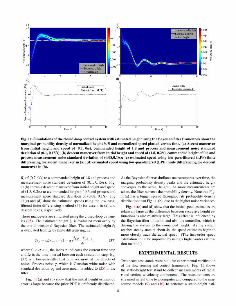
Fig. 11. Simulations of the closed-loop control system with estimated height using the Bayesian filter framework show themarginal probability density of normalized height h/R and normalized speed plotted versus time. (a) Ascent maneuverfrom initial height and speed of (0.7, 0/s), commanded height of 1.8 and process and measurement noise standarddeviation of (0.1, 0.15/s); (b) descent maneuver from initial height and speed of (1.8, 0.2/s), commanded height of 0.6 andprocess measurement noise standard deviation of (0.08,0.1/s); (c) estimated speed using low-pass-filtered (LPF) finitedifferencing for ascent maneuver in (a); (d) estimated speed using low-pass-filtered (LPF) finite differencing for descentmaneuver in (b).

R) of (0.7, 0/s) to a commanded height of 1.8 and process andmeasurement noise standard deviation of (0.1, 0.15/s). Fig.11(b) shows a descent maneuver from initial height and speedof (1.8, 0.2/s) to a commanded height of 0.6 and process andmeasurement noise standard deviation of (0.08, 0.1/s). Fig11(c) and (d) show the estimated speeds using the low-pass-filtered finite-differencing method (37) for ascent in (a) anddescent in (b), respectively.

These manuevers are simulated using the closed-loop dynam-ics (25). The estimated height z1 is evaluated recursively bythe one-dimensional Bayesian filter. The estimated height z2is evaluated from z1 by finite differencing, i.e.,

z2,p = α z2,p−1 +(1−α)z1,p− z1,p−1

∆t, (37)

where 0 < α < 1, the index p indicates the current time stepand ∆t is the time interval between each simulation step. Eq.(37) is a low-pass-filter that removes most of the effects ofnoise. Process noise γ , which is Gaussian white noise withstandard deviation σγ and zero mean, is added to (25) in thefilter.

Fig. 11(a) and (b) show that the initial height estimationerror is large because the prior PDF is uniformly distributed.

As the Bayesian filter assimilates measurements over time, themarginal probability density peaks and the estimated heightconverges to the actual height. As more measurements aretaken, the filter narrows the probability density. Note that Fig.11(a) has a bigger spread throughout its probability densitydistribution than Fig. 11(b), due to the higher noise variances.

Fig. 11(c) and (d) show that the initial speed estimates arerelatively large as the difference between succesive height es-timations is also relatively large. This effect is influenced bythe Bayesian filter initiation and also the controller, which isdriving the system to the comanded height. As the systemreaches steady state at about 4s, the speed estimates begin tomore closely track the actual speed. (The first-order speedestimation could be improved by using a higher-order estima-tion method.)

EXPERIMENTAL RESULTS

Two heave test stands were built for experimental verificationof the flow-sensing and control framework. Fig. 12 showsthe static-height test stand to collect measurements of radialv and vertical w velocity components. The measurements arestreamed in real time to a computer and compared to the ring-source models (9) and (10) to generate a static-height esti-

8

mate. Fig. 9 shows the compound pendulum heave test standused to verify the dynamics and closed-loop control.

Fig. 12. Static-height test stand.

Table 1. Experimental Equipment.Equipment Model & MakeBrushless Direct Circuit Motor 850Kv AC2830-358Differential Pressure Sensors Honeywell

HSCDRRN001NDAA3Direct Circuit Power Supply Mastech HY3030EElectronic Speed Controller eRC Rapid Drive 25AModular Aluminum Profiles MakerBeam & 8020Microcontroller: Cortex-M4 Teensy 3.1

Data AcquisitionMicrocontroller: ATmega328

Motor Speed Arduino NanoOptical Tachometer Neiko 20713ARemote Control Radio Spektrum DX6iRotor HobbyKing 14X4.7

Carbon FiberScale Ohaus Valor 100

Table 1 lists the make and model of the experimentalequipment. Fig. 13 shows the instrumentation setup, whhis common to both test stands. Note that the Remote Control(RC) radio is used for manual motor-speed control, whereasthe Arduino Nano microcontroller is used for automatic speedcontrol.

An airspeed probe set that is capable of measuring the ra-dial and vertical velocity components consists of two pairs oftubes. Each pair is connected to a differential pressure sen-sor (Ref. 12). The pressure sensors are connected via an ana-log interface to the Teensy 3.1 Microcontroller for Data Ac-quisition (DAQ). Since the pressure measurements are rela-tively noisy and the pressure sensor and DAQ microcontrollerare capable of higher data rates than the estimation and controlloop in the computer, a Moving Average Filter (MAF) is im-plemented on the pressure measurements to generate velocity

Fig. 13. Test stand instrumentation.

measurements V . The MAF implementation is

V =pJ

J

∑j=1

Pj, (38)

where Pj is the instantaneous measurement from the differen-tial pressure sensor, J is the number of datapoints to averageover and p is the conversion factor from differential pressureto velocity (Ref. 12).

The actuation of the experimental setup consists of aBrushless Direct Circuit (BLDC) motor and Electronic SpeedController (ESC) pair. Speed-control input requires PulseWidth Modulation (PWM) square wave signals with variabletimescales, which are generated by the RC receiver or Ar-duino Nano microcontroller.

Fig. 14. Comparison between ring-source potential flowmodels (9), (10) and experimental results of radial v andvertical w velocity components for various radial loca-tions. Normalized height z/R = 0.75, normalized sensorlocation (z/R)sensor= 0.18, rotational speed ω=2538 RPM,induced velocity IGE vi,IGE = 4.34m/s.

Verification of Flow Model and Height Estimation Frame-work

Fig. 14 compares the measured radial and vertical velocitycomponents with the flow model at normalized height z/R

9

Fig. 15. Static height estimation at normalized heightz/R=0.75 for verification of ring-source potential flowmodels (9) and (10) using measured radial v and ver-tical w velocity components. Normalized sensor loca-tion (r/R,z/R)sensor= (0.75,0.18), rotational speed ω=2538RPM, induced velocity IGE vi,IGE = 4.34m/s.

Fig. 16. Rotor Thrust Test Setup.

= 0.75, with the sensors placed 0.18R away from the rotorplane, motor rotational speed of 2538 RPM and induced ve-locity IGE vi,IGE of 4.34 m/s. The induced velocity IGE is theaverage of vertical velocities close to the rotor plane acrossmultiple radial locations and, in this case, zsensor/R= 0.05.

The radial velocity crosses over from positive to negativeat r/R=0.75, which represents suction toward the rotor hub.The model does not predict this outcome due to the geometryof the ring sources because inward flow at opposite sides ofthe same ring cancel out and radial velocity is always outwardand positive. Furthermore, the radial flow is also influencedby turbulence and the tip vortices of each rotor blade, whereasthe flow model captures only the mean velocity. The flowmodel underpredicts the vertical velocity component, whichis likely because the induced velocity is an average rather thanlocal value.

Fig. 15 shows the static height-estimation results at nor-malized height z/R = 0.75 and normalized sensor locations at(r,z)sensor/R = (0.75, 0.18). The difference between the es-timated height and the actual height has 13.8% mean error.Observed that the vertical velocity is relatively stable and theestimation errors are primarily caused by fluctuations in the

Fig. 17. Thrust T and rotational speed ω relationship outof Ground Effect, comparing a curve fit and model (13)against experimental results.

Fig. 18. Normalized height z/R and rotational speed ω atsteady-state in Ground Effect.

radial velocity.

Open-Loop and Motor Dynamics

Fig. 16 shows the thrust test setup used to measure the rela-tionship between rotor thrust T and rotational speed ω OGE.The motor-ESC pair is mounted on the test stand, which iscoupled with the scale. The DC Power Supply powers themotor-ESC pair and the Remote Control (RC) receiver con-trols the motor rotational speed. The rotor is mounted so thatthe thrust vector points downwards into the scale. This ar-rangement is primarily to facilitate operation OGE such thatthe ground does not impinge on the rotor downwash.

Fig. 17 shows the relationship between thrust and rota-tional speed OGE. The thrust model (13), including only sec-ond order terms (ω2), is compared with experimental resultsand a curve-fit approach of both first and second order terms(ω and ω2). The thrust model fits the experimental resultswell on the lower rotational speeds and slightly overpredictsthrust on higher rotational speeds, whereas the curve-fit ap-proach does the opposite. Since we are operating in the lowerrotational speed regions around 3000–4000 RPM, as shownlater in Fig. 18, the choice of the thrust model is justified.Note that ignoring the first order term also simplifies the dy-namics (15).

10

Fig. 19. Normalized height z/R versus time in Ground Ef-fect for various rotor rotational speeds starting from rest.

Fig. 18 shows the steady-state open-loop dynamics of thecompound-pendulum heave test stand by plotting the relation-ship between normalized height z/R and rotational speed ω atsteady-state. The height was measured by a Qualisys MotionCapture setup. The compound-pendulum heave test stand isat rest at z/R = 0.5 and reaches its maximum height at z/R =2.35. The plot depicts a highly nonlinear relationship with theheight rising slowly at first up to 3447 RPM. From 3500 to3865 RPM, each incremental increase in rotational speed re-sults in a significant increase in height. The steep slope of thiscurve is a characteristic of the ESC-motor combination anda change of this combination could result in a more gradualresponse.

Fig. 19 shows the open-loop normalized height for variousrotor rotational speeds starting from rest. There is a generaltrend of a steep increase in the height corresponding to thecommanded input and the height decreases to the steady-statevalue. As the rotational speed increases, it takes longer beforethe motor-ESC pair converges to the steady-state height. Theincreased settling time as rotational speed increases is due tothe large difference between commanded rotational speed andrest. A smaller rotational speed difference will decrease thesettling time.

At lower rotational speeds, the dynamics seem to be over-damped. At higher rotational speeds, oscillations of the dy-namics model (32) are evident. The delayed convergenceto steady-state height and height oscillations suggest that themotor-ESC dynamics introduce a time constant τ . The motor-ESC dynamics are modeled as (Ref. 24)

τω +ω = fmot(u), (39)

where ω is the rotational acceleration and fmot is the nonlinearrotational speed response as a function of the PWM commandinput u. In ongoing work, the closed-loop controller combines(39) with the compound-pendulum test stand dynamics (32).

CONCLUSIONS

This paper describes a dynamic controller for rotorcraft land-ing and hovering in ground effect. A ring-source flow modelfor the rotor downwash IGE developed using potential flow

theory captures the essential characteristics of the relation-ship between flow velocity and height. The reduced-orderflow model used for fast evaluation of the flowfield in a recur-sive control loop has been experimentally validated. A non-linear dynamic model of rotorcraft landing IGE allows for thestudy of the open-loop dynamics and facilitates the design ofa closed-loop controller. Both the steady-state and transientopen-loop dynamics of the compound-pendulum heave testsetup are experimentally investigated; a model of the motordynamics is proposed. The height of the rotorcraft IGE is ex-perimentally estimated with a grid-based recursive Bayesianfilter using the three-dimensional flow model, nonlinear dy-namic model and differential pressure probe measurements.Finally, flow-estimation-based closed-loop control is imple-mented in simulation, demonstrating that height estimationand control is possible using only flow sensors. Experimentalvalidation of the closed-loop system is ongoing.

ACKNOWLEDGMENTS

The authors gratefully thank William Craig, Derrick Yeo,Daigo Shishika, and Nitin Sydney for valuable discussionsand assistance. This work is supported by the University ofMaryland Vertical Lift Rotorcraft Center of Excellence ArmyGrant No. W911W61120012.

REFERENCES1Tritschler, J., “Contributions to the Characterization and

Mitigation of Rotorcraft Brownout,” Doctor of PhilosophyDissertation, Department of Aerospace Engineering, Univer-sity of Maryland, 2012.

2Plank, V.G., Spatola, A.A., Hicks, J.R., “Fog Modifica-tion by Use of Helicopters,” Air Force Cambridge ResearchLaboratories, U.S. Army Atmospheric Sciences Laboratory,AFCRL-70-0593, Environmental Research Papers No. 335,ECOM-5339, October 28, 1970.

3Serra, P., Cunha, R., Silvestre, C., “On the Design of Ro-torcraft Landing Controllers,” 16th Mediterranean Confer-ence on Control and Automation Ajaccio, France, June 25-27,2008.

4Mahony, R., Hamel, T., “Adaptive Compensation of Aero-dynamic Effects during Takeoff and Landing Manoeuvres fora Scale Model Autonomous Helicopter,” European Journal ofControl, (2001)0:1-15, 2001.

5Nonaka, K., Sugizaki, H., “Integral Sliding Mode AltitudeControl for a Small Model Helicopter with Ground EffectCompensation,” American Control Conference, San Fran-cisco, CA, June 29 - July 01, 2011.

6Borenstein, J., Koren, Y., “Obstacle Avoidance with Ultra-sonic Sensors,” IEEE Journal for Robotics and Automation,Vol. 4, No. 2, April 1988.

11

7Tanigawa, M., Luinge, H., Schipper, L., Slycke, P., “Drift-Free Dynamic Height Sensor using MEMS IMU Aided byMEMS Pressure Sensor,” Proceedings of the 5th Workshopon Positioning, Navigation and Communication, 2008.

8Prouty, R.W., Helicopter Performance, Stability, and Con-trol, Krieger Publishing Company, Florida, 2002.

9Gilad, M., Chopra, I., Rand, O., “Performance Evaluationof a Flexible Rotor in Extreme Ground Effect,” 37th EuropeanRotorcraft Forum, Milan, Italy, 2011.

10Govindarajan, B., “Evaluation of Particle Clustering Algo-rithms in the Prediction of Brownout Dust Clouds,” Master’sThesis, Department of Aerospace Engineering, University ofMaryland, August 2011.

11Cheeseman, I.C., Bennett, W.E., “The Effect of the Groundon a Helicopter Rotor in Forward Flight,” Reports & Memo-randa No. 3021, Ministry of Supply, Aeronautical ResearchCouncil Reports and Memoranda, September 1955.

12Yeo, D. W., Sydney, N., Paley, D., Sofge, D., “OnboardFlow Sensing For Downwash Detection and Avoidance OnSmall Quadrotor Helicopters,” AIAA Guidance, Navigationand Control Conference 2015, accepted for publication.

13Lagor, F.D., DeVries, L.D., Waychoff, K., Paley, D.A.,“Bio-inspired Flow Sensing and Control: Autonomous Rheo-taxis Using Distributed Pressure Measurements,” Journal ofUnmanned System Technology, Nov 2013.

14DeVries, L.D., Lagor, F.D., Lei, H., Tan, X. ,Paley, D.A.,“Distributed Flow Estimation and Closed-Loop Control ofan Underwater Vehicle with a Multi-Modal Artificial LateralLine,” Bioinspiration & Biomimetics, special issue on “Hy-brid and Multi-modal Locomotion,” accepted for publication.

15Hooi, C.G., Lagor, F. , Paley, D., “Flow Sensing, Esti-mation and Control for Rotorcraft in Ground Effect,” IEEEAerospace Conference, Big Sky, Montana, March 2015.

16Hooi, C.G., “Design, Rapid Prototyping and Testing ofa Ducted Fan Microscale Quadcopter,” 70th American Heli-copter Society Society Annual Forum & Technology Display,Montreal, Quebec, Canada, May 2014.

17Leishman, J.G., Principles of Helicopter Aerodynamics,2nd. Ed., p.258 - 260, Cambridge University Press, New York,2006.

18Hess, J.L., Smith, A.M.O., “Calculation of Potential Flowabout Arbitrary Bodies,” Progress in Aerospace Sciences, Vol-ume 8, p. 3940, 1967.

19Lee, T.E., Leishman, J.G., Ramasamy, M., “Fluid Dynam-ics of Interacting Blade Tip Vortices with a Ground Plane,”Journal of the American Helicopter Society 55, 022005, 2010.

20Murphy, K., Machine Learning: A Probabilistic Perspec-tive, The MIT Press, Cambridge, Massachusetts, London,2012.

21Simon, D., Optimal State Estimation: Kalman, H Infinity,and Nonlinear Approaches , 1st. Ed., p.465-466, John Wiley& Sons, Inc., New Jersey, 2006.

22Arulampalam, M.S., Maskell, S., Gordon, N., Clapp, T.,“A Tutorial on Particle Filters for Online Nonlinear/Non-Gaussian Bayesian Tracking,” IEEE Transactions on SignalProcessing, Vol. 50, No. 2, February 2002.

23Julier, S., Uhlmann, J., “Unscented Filtering and NonlinearEstimation”, Proceedings of the IEEE, Vol. 92, No. 3, March2004.

24Petru, E.S., “Intelligent Control and Cooperation for Mo-bile Robots,” Doctor of Philosophy Dissertation, Universityof Texas at Arlington, December 2011.

12