Flow Shop Scheduling

with Earliness, Tardiness and

Intermediate Inventory Holding Costs

Kerem Bulbul∗

Philip Kaminsky

Candace Yano

Industrial Engineering and Operations Research

University of California, Berkeley, CA

May 2003

Abstract

We consider the problem of scheduling customer orders in a flow shop with the objective of minimizing

the sum of tardiness, earliness (finished goods inventory holding) and intermediate (work-in-process)

inventory holding costs. We formulate this problem as an integer program, and based on approximate

solutions to two different, but closely related, Dantzig-Wolfe reformulations, we develop heuristics to

minimize the total cost. We exploit the duality between Dantzig-Wolfe reformulation and Lagrangian

relaxation to enhance our heuristics. This combined approach enables us to develop two different lower

bounds on the optimal integer solution, together with intuitive approaches for obtaining near-optimal

feasible integer solutions. To the best of our knowledge, this is the first paper that applies column

generation to a scheduling problem with different types of strongly NP-hard pricing problems which are

solved heuristically. The computational study demonstrates that our algorithms have a significant speed

advantage over alternate methods, yield good lower bounds, and generate near-optimal feasible integer

solutions for problem instances with many machines and a realistically large number of jobs.

∗Corresponding author. E-mail: bulbul@ieor.berkeley.edu.

1

1 Introduction

We address the problem of scheduling flow shops in settings with penalties (explicit or implicit) for tardiness

in delivering customer orders, as well as costs for holding both finished goods and work-in-process inventory.

Our work was motivated, in part, by applications in the biotechnology industry. The vast majority of

biotechnology products require a well-defined series of processing steps, and processing usually occurs in

batches, at least until the final packaging steps. Thus, in many instances, the manufacturing arrangement

may be accurately characterized as a flow shop, with batches moving from one process to the next.

The scheduling of the various process steps is complicated by the relative fragility of these products

between successive processing stages. Delays between stages increase the chances of contamination or de-

terioration. Some products require refrigeration and storage in other types of specially-controlled facilities

that are expensive to build and maintain. For instance, the authors are aware of an example in which

live blood cells are used to generate certain blood components that are extracted and further processed in

the manufacture of a treatment for a particular blood disorder. Sterile conditions are essential throughout

the process, including during any waiting between stages. At various work-in-process stages, the product

requires very precise temperature control, physical separation of batches, etc. Thus, the cost of holding

work-in-process inventory can be substantial, and at some stages, may greatly exceed the cost of holding

finished goods inventory.

There are also “low-tech” examples in which intermediate inventory holding costs are important and

quite different in value from finished goods holding costs. For example, the steel used in automobile body

parts is coated (to delay corrosion) before the steel is blanked (cut) and stamped into the proper shapes.

Until the blanking stage, the steel is held in the form of coils and is relatively compact. After coating, the

product is more stable (less subject to corrosion) than before coating, so the inventory holding costs may

be lower after coating. On the other hand, after the parts are stamped, they must be stored in containers

or racks, and require significantly more space than the equivalent amount of steel in coil form. This is an

instance in which total earliness (at all stages) is not a reliable indicator of the cost of holding inventory,

and distinguishing among inventory at different stages is important in making good scheduling decisions.

Problems with earliness (finished goods holding) costs and tardiness costs have been studied extensively

in single-machine contexts. (See Kanet and Sridharan (2000) and references therein). Also, many results

exist for parallel machine earliness/tardiness scheduling problems, especially when all jobs have the same

due date. (See Sundararaghavan and Ahmed (1984), Kubiak et al. (1990), Federgruen and Mosheiov (1996),

Chen and Powell (1999a) and Chen and Powell (1999b).) However, relatively little research has been done

on flow- and job shop environments when earliness and tardiness costs are present in the objective function.

Some examples include Sarper (1995) and Sung and Min (2001) who consider 2-machine flow shop common

due date problems, and Chen and Luh (1999) who develop heuristics for a job shop weighted earliness and

2

tardiness problem. Work-in-process inventory holding costs have been explicitly incorporated in Park and

Kim (2000), Kaskavelis and Caramanis (1998), and Chang and Liao (1994) for various flow- and job shop

scheduling problems, although these papers consider different objective functions and approaches than ours.

For complex scheduling problems, a common approach involves decomposing the original problem into

a set of independent subproblems by relaxing some of the constraints. The aim is to achieve a decompo-

sition in which the subproblems are relatively easy to solve, and to use the collective solution from these

subproblems as the basis for constructing an effective solution for the original problem. These decomposition

methods include traditional mathematical programming decomposition methods, including Lagrangian re-

laxation (LR) and Dantzig-Wolfe (DW) decomposition, as well as decomposition methods that were designed

specifically for scheduling problems, such as shifting bottleneck algorithms. In this paper, we develop two

different Dantzig-Wolfe reformulations of the problem described above, and solve them using column genera-

tion enhanced by Lagrangian relaxation and use of artificial variables in the linear programming (LP) master

problems. We also construct high quality feasible solutions for the original problem from the information

in the solution of the Dantzig-Wolfe reformulations. In Section 3, we first describe our initial approach and

then discuss in detail each of the modifications to the column generation algorithm.

Column generation has recently been applied successfully to a variety of scheduling problems. Van den

Akker et al. (2000) develop a framework for the Dantzig-Wolfe reformulation of time-indexed formulations

of machine scheduling problems and apply it to the single-machine weighted completion time problem with

unequal ready times. Van den Akker et al. (2002) report that the LP relaxation of their set covering

formulation of the single-machine unrestrictive common due date problem with asymmetric weights yields

the optimal integer solution in all of their randomly generated instances. Chen and Powell (1999a), Chen

and Powell (1999b), Van den Akker et al. (1999a), Lee and Chen (2000) and Chen and Lee (2002), among

others, have developed column generation methods for parallel machine scheduling problems. In particular,

Chen and Powell (1999a) and Chen and Lee (2002) consider two parallel machine scheduling problems with

the objective of minimizing the total weighted earliness and tardiness. In both cases, a set partitioning

formulation is solved by column generation. In the first paper, there is a common unrestrictive due date for

all jobs, and in the second, the authors consider a common due window which may have a restrictively small

starting point.

When decomposition approaches are employed for parallel machine scheduling, the subproblems are

typically identical, or of similar form. In our flow shop scheduling problem, however, the subproblems may be

quite different from each other; nevertheless, we develop an algorithm that can solve all of them effectively. In

all of the parallel machine scheduling problems mentioned above, the pricing problems are pseudo-polynomial

and solved optimally by a dynamic programming algorithm. To the best of our knowledge, this paper is

the first attempt to apply column generation to a machine scheduling problem where some subproblems

are strongly NP-hard. (See Section 3.) In Section 5, we demonstrate computationally that approximate

3

solutions for the subproblems do not compromise the overall solution quality. Furthermore, we are able to

derive insights from the complementary properties of Dantzig-Wolfe reformulation and Lagrangian relaxation

with little additional effort. Recently, Van den Akker et al. (2002) combined Lagrangian relaxation with

column generation in order to solve a single-machine common due date problem. The authors enhance

their column generation algorithm in several ways by obtaining an alternate lower bound from Lagrangian

relaxation, and by tuning their LP master problem formulation based on insights from the Lagrangian

model. The algorithm of Cattrysse et al. (1993), who improve the values of the dual variables from the

optimal solution of the restricted LP master problem by performing Lagrangian iterations before solving

the pricing problems, is in some sense similar to our approach in Section 3.3, although we do not pass dual

variables from Lagrangian relaxation to column generation. In addition, Dixon and Poh (1990) and Drexl

and Kimms (2001) consider Dantzig-Wolfe reformulation and Lagrangian relaxation as alternate methods,

but do not use both approaches together.

The key to developing effective decomposition approaches is finding a “good” set of coupling constraints

to relax. On one hand, the relaxed problem needs to be relatively easy to solve, but on the other, it should

provide a reasonable approximation of the original problem. Typically, there is a trade-off between these

two goals. Relatively easy subproblems frequently imply looser bounds, and thus less useful information for

solving the original problem. In this paper, we relax the operation precedence constraints, as opposed to

the machine capacity constraints that are most frequently relaxed in the scheduling literature. Although

this approach results in more difficult subproblems, we solve these approximately and obtain effective so-

lutions for the original problem. See Fisher (1971) for a general discussion of Lagrangian approaches to

resource-constrained scheduling problems in which capacity constraints are relaxed. More recent examples

of Lagrangian algorithms can be found in Chang and Liao (1994) and Kaskavelis and Caramanis (1998).

Note that Van de Velde (1990) and Hoogeveen and van de Velde (1995) apply Lagrangian relaxation to

the 2-machine flow shop total completion time problem with equal ready times by relaxing the operation

precedence constraints, and solve this problem effectively by developing polynomial algorithms for their

subproblems. Also, Chen and Luh (1999) solve a job shop total weighted earliness/tardiness problem by

Lagrangian relaxation where the operation precedence constraints are relaxed. In their model, there may be

several machines of the same type, and thus their subproblems are parallel machine total weighted completion

time problems, which are solved approximately. They compare their approach to an alternate Lagrangian

relaxation algorithm where machine capacity constraints are relaxed. Their results indicate that relaxing

operation precedence constraints yields superior results in memory and computation time, especially when

the due dates are not tight.

In this paper, we develop heuristics for the m-machine flow shop earliness/tardiness scheduling problem

with intermediate inventory holding costs based on the LP relaxation of its Dantzig-Wolfe reformulation

solved approximately by column generation. We compare two different reformulations in which the column

4

generation scheme is enhanced by the solution of an equivalent Lagrangian relaxation formulation and use

of artificial variables in the LP master problem. The subproblems are solved heuristically. From tight

lower bounds for the subproblems, we develop two different lower bounds for the overall problem. Addition-

ally, from the approximate solution of the LP relaxation of the Dantzig-Wolfe reformulation, we develop a

technique to construct good feasible solutions for the original problem.

In Section 2, we present a formal description of the problem, and discuss complexity and modeling

issues. In Section 3, we develop the mathematical models, explain how we combine column generation

and Lagrangian relaxation, present our lower bounds, and the heuristics to obtain feasible integer solutions

from the (not necessarily optimal) solution of the Dantzig-Wolfe decomposition. In Section 4, we discuss

the various steps of our column generation algorithm, including an effective approach for the subproblems.

Finally, in Section 5 we present computational results, and in Section 6, we conclude and discuss future

research directions.

2 Problem Description

Consider a non-preemptive flow shop with m machines in series and n jobs. Each job visits the machines

in the sequence i = 1, . . . , m and is processed without preemption on each machine. We do not require a

permutation sequence, i.e., the sequence of jobs may differ from one machine to another. Associated with

each job j, j = 1, . . . , n, are several parameters: pij , the processing time for job j on machine i; rj , the

ready time of job j; dj , the due date for job j; hij , the holding cost per unit time for job j while it is waiting

in the queue before machine i; εj , the earliness cost per unit time if job j completes processing on the final

machine before time dj ; and πj , the tardiness cost per unit time if job j completes processing on the final

machine after time dj . All ready times, processing times and due dates are assumed to be integer.

The objective is to determine a feasible schedule that minimizes the sum of costs across all jobs. For a

given schedule S, let Cij be the time at which job j finishes processing on machine i, and wij be the time job

j spends in the queue before machine i. The sum of costs for all jobs in schedule S, C(S), can be expressed

as follows:

C(S) =n∑

j=1

h1j(C1j − p1j − rj) +m∑

i=2

n∑j=1

hijwij +n∑

j=1

εjEj + πjTj , (2.1)

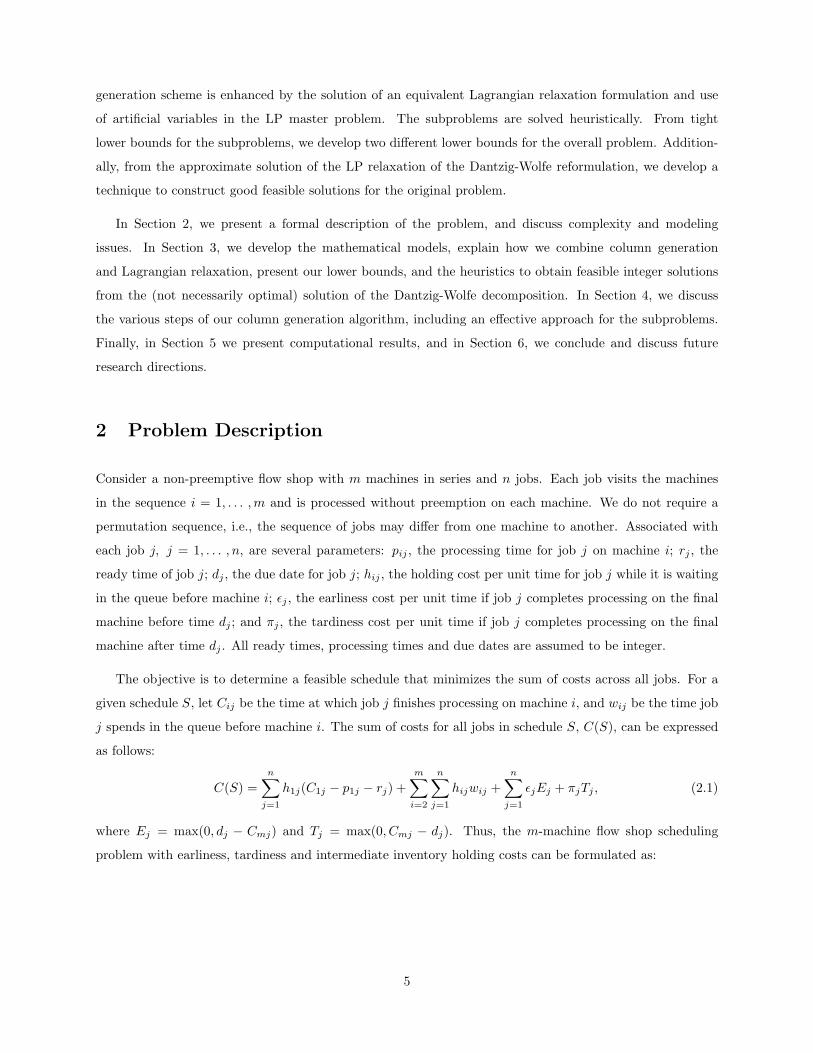
where Ej = max(0, dj − Cmj) and Tj = max(0, Cmj − dj). Thus, the m-machine flow shop scheduling

problem with earliness, tardiness and intermediate inventory holding costs can be formulated as:

5

(Fm)

zFm = minS

C(S) (2.2)

s.t.

C1j ≥ rj + p1j ∀j (2.3)

Ci−1j − Cij + wij = −pij i = 2, . . . ,m, ∀j (2.4)

Cik − Cij ≥ pik or Cij − Cik ≥ pij ∀i, j, k (2.5)

Cmj + Ej − Tj = dj ∀j (2.6)

wij ≥ 0 i = 2, . . . , m, ∀j (2.7)

Ej , Tj ≥ 0 ∀j (2.8)

The constraints (2.3) prevent processing of jobs before their respective ready times on machine one. Con-

straints (2.4), referred to as operation precedence constraints, ensure that jobs follow the processing sequence

machine 1, machine 2,..., machine m. Machine capacity constraints (2.5) ensure that a machine processes

only one job at a time, and a job is finished once started. Constraints (2.6) relate the completion times

on the final machine to earliness and tardiness values. In the rest of the paper, zM denotes the optimal

objective function value of a model M, where M refers to any of the models we consider.

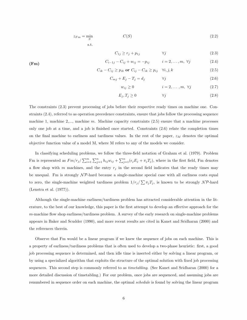
In classifying scheduling problems, we follow the three-field notation of Graham et al. (1979). Problem

Fm is represented as Fm/rj/∑m

i=1

∑nj=1 hijwij +

∑nj=1(εjEj + πjTj), where in the first field, Fm denotes

a flow shop with m machines, and the entry rj in the second field indicates that the ready times may

be unequal. Fm is strongly NP-hard because a single-machine special case with all earliness costs equal

to zero, the single-machine weighted tardiness problem 1/rj/∑

πjTj , is known to be strongly NP-hard

(Lenstra et al. (1977)).

Although the single-machine earliness/tardiness problem has attracted considerable attention in the lit-

erature, to the best of our knowledge, this paper is the first attempt to develop an effective approach for the

m-machine flow shop earliness/tardiness problem. A survey of the early research on single-machine problems

appears in Baker and Scudder (1990), and more recent results are cited in Kanet and Sridharan (2000) and

the references therein.

Observe that Fm would be a linear program if we knew the sequence of jobs on each machine. This is

a property of earliness/tardiness problems that is often used to develop a two-phase heuristic: first, a good

job processing sequence is determined, and then idle time is inserted either by solving a linear program, or

by using a specialized algorithm that exploits the structure of the optimal solution with fixed job processing

sequences. This second step is commonly referred to as timetabling. (See Kanet and Sridharan (2000) for a

more detailed discussion of timetabling.) For our problem, once jobs are sequenced, and assuming jobs are

renumbered in sequence order on each machine, the optimal schedule is found by solving the linear program

6

TTFm below.

(TTFm)

zTTFm = minCij

C(S) (2.9)

s.t.

(2.3)− (2.4) and (2.6)− (2.8)

Cij − Cij−1 ≥ pij ∀i, j = 2, . . . , n (2.10)

In our approach, we reformulate Fm, solve its linear programming relaxation approximately, construct job

processing sequences on each machine from this solution, and find the optimal schedule given these sequences

by solving TTFm. The strength of our algorithm lies in its ability to identify near-optimal job processing

sequences.

In Fm, the machine capacity constraints are modeled as a set of disjunctive constraints (2.5), and we

have to specify a mechanism such that exactly one of each pair of constraints is imposed depending on the

job sequence. One approach is to introduce binary variables δijk, such that δijk = 1 if job j precedes job k

on machine i, and zero otherwise. Then, we can add the following constraints to Fm and drop (2.5) from

the formulation, where M is a large enough constant.

Cij − Cik ≥ pij −Mδijk ∀i, j, k (2.11)

δijk ∈ {0, 1} ∀i, j, k (2.12)

Unfortunately, in the linear programming relaxation of Fm, the constraints (2.11) are not binding and the

bound obtained is loose. Recall that we are interested in near-optimal feasible integer solutions, and for this

purpose, we require a relatively tight LP relaxation.

Dyer and Wolsey (1990) introduced time-indexed formulations of scheduling problems. These formula-

tions have attracted much attention in recent years because they often have strong LP relaxations, and they

frequently play an important role in approximation algorithms for certain classes of scheduling problems.

For instance, Goemans et al. (1999) and Schulz and Skutella (1997) use time-indexed formulations to develop

approximation algorithms for 1/rj/∑

βjCj and R/rj/∑

βjCj , respectively, where R in the first field stands

for unrelated parallel machines. In time-indexed formulations, job finish times are represented by binary

variables, and constraints such as (2.5) are replaced by a large set of generalized upper bound constraints

which tighten the formulation. (For details, see Dyer and Wolsey (1990), Sousa and Wolsey (1992) and

Van den Akker et al. (1999b).) In general, the major disadvantage of time-indexed formulations is their size

which grows rapidly with the number of jobs and the length of the processing times. (See the survey by

Queyranne and Schulz (1994).)

The concept of time-indexed formulations is relevant to our approach for several reasons. First, in

Proposition 3.11 we show that the Dantzig-Wolfe reformulation of the time-indexed formulation for our

7

problem (see TIFm below) is the same as that of Fm. This implies that the optimal objective function

value of the LP relaxation of our Dantzig-Wolfe reformulation is at least as large as the optimal objective

function value of the LP relaxation of TIFm. Also, we use the LP relaxation of TIFm as a benchmark in

our computational study to demonstrate that our heuristic approach has a significant speed advantage, with

little compromise in solution quality.

In order to present the time-indexed formulation for our problem, let tij = rij + pij represent the earliest

possible time job j can finish on machine i, where the operational ready time rij of job j on machine i is defined

as rij = rj +∑i−1

l=1 plj , and r1j = rj . Note that tmax = maxj max(rj , dj) + P , where P =∑m

i=1

∑nj=1 pij is

the sum of processing times on all machines, is the latest time that any job could conceivably be finished in

an optimal schedule, accounting for potential idle time. Thus, let the latest time job j can finish on machine

i be tij = tmax −∑m

l=i+1 plj , and define the processing interval for job j on machine i as Hij = {k ∈ Z|tij ≤

k ≤ tij}. Similarly, the processing interval for machine i is defined as Hi = {k ∈ Z|minj tij ≤ k ≤ maxj tij}.

Finally, let xijk equal one if job j finishes processing on machine i at time k, and zero otherwise. The

time-indexed formulation is:

(TIFm)

zTIFm = minxijkwij

n∑j=1

∑k∈H1j

h1j(k − p1j − rj)x1jk (2.13)

+m∑

i=2

n∑j=1

hijwij

+n∑

j=1

∑k∈Hmj

k≤dj

εj(dj − k) +∑

k∈Hmjk>dj

πj(k − dj)

xmjk

s.t. ∑k∈Hij

xijk = 1 ∀i, j (2.14)∑k∈Hi−1j

kxi−1jk −∑

k∈Hij

kxijk + wij = −pij i = 2, . . . , m,∀j (2.15)

n∑j=1

∑t∈Hij

k≤t≤k+pij−1

xijt ≤ 1 ∀i, k ∈ Hi (2.16)

xijk ∈ {0, 1} ∀i, j, k ∈ Hij (2.17)

wij ≥ 0 j = 2, . . . , m,∀j (2.18)

Constraints (2.14) ensure that each job is processed exactly once on each machine. The generalized upper

bound constraints (2.16) ensure that each machine processes at most one job at any time. Observe that

the operation precedence constraints (2.15) are equivalent to the operation precedence constraints (2.4) in

Fm because there is exactly one k ∈ Hij for which xijk = 1, and thus∑

k∈Hijkxijk = Cij . Note that

these constraints introduce coefficients with value O(tmax) into the constraint matrix. One can also consider

an alternate, potentially tighter formulation as follows: drop wij from the formulation, introduce binary

variables wijk that take the value one if job j is waiting in queue before machine i at time k and zero

8

otherwise, make the appropriate changes to the objective function, and replace constraints (2.15) with the

following: ∑t∈Hi−1j

t≤k

xi−1jt − wij(k+1) =∑

t∈Hijt≤k+pij

xijt i = 2, . . . , m,∀j, k ∈ Hi−1j (2.19)

wijk ≥ 0 ∀i, j, k ∈ Hi−1j \ {ti−1j} ∪ {ti−1j + 1} (2.20)

As we mentioned previously, time-indexed formulations can grow very rapidly with the number of jobs.

Indeed, in TIFm there are O(2mn + mtmax) constraints, but if (2.15) is replaced by (2.19), then there are

O(mn + m(n + 1)tmax) constraints, which simply becomes unmanageable. For this reason, we have elected

to utilize a formulation that includes a single operation precedence constraint per job per machine, and in

the next section we explain our solution approach for this formulation.

3 Solution Approach

In this section, first we present the Dantzig-Wolfe reformulation of Fm, as well as the corresponding La-

grangian relaxation model, and then we discuss how we can exploit the duality between these two approaches.

In fact, our observations concerning the subproblem and the Lagrangian objective functions lead us to an

alternate DW reformulation and the corresponding LR model.

Both of the alternate DW reformulations can be used to solve the m-machine flow shop earliness/tardiness

scheduling problem with intermediate inventory holding costs, but the convergence is slow when we solve

these DW reformulations with column generation. We note that this “tailing-off” effect is rooted in the

relative magnitudes of the dual variables and the inventory holding costs, and we explain this phenomenon

by using the “shadow price” interpretation of the dual variables. Furthermore, we develop a two-phase

algorithm that alleviates this “tailing-off” effect to a great extent. In the first phase, artificial variables

are introduced into the DW reformulation to impose a structure on the dual variables which speeds up the

convergence. The artificial variables are eventually driven to zero in the second phase.

3.1 Initial Models

First DW Reformulation

We formulate the m-machine flow shop earliness/tardiness scheduling problem with intermediate inventory

holding costs as an integer programming problem with an exponential number of variables that represent

capacity-feasible schedules for individual machines. Although there is an infinite number of capacity-feasible

schedules on each machine if the completion times are continuous variables, the last job on the last machine

will finish at or before tmax in any optimal solution to our problem. Furthermore, by the integrality of ready

9

times, due dates and processing times, there exists an optimal solution in which all completion times are inte-

gral. Thus, without loss of generality, we can assume that the number of possible schedules on each machine

is finite but exponential. Additionally, we require that these capacity-feasible schedules satisfy the operational

ready time constraints, Cij ≥ rij + pij . Let the set of all schedules on machine i be denoted by Si. Each of

these schedules Ski , k = 1, . . . , Ki, where Ki = |Si|, is defined by a set of completion times {Ck

ij}, i.e., Ski =

{Ckij ∈ Z, j = 1, . . . , n| tij ≤ Ck

ij ≤ tij ∀j, and Ckij , j = 1 . . . , n, satisfy capacity constraints on machine i}.

Let xki be a binary variable that takes the value one if we choose Sk

i on machine i, zero otherwise. The earliness

and tardiness of job j in schedule Skm are computed as Ek

j = max(0, dj −Ckmj), and T k

j = max(Ckmj −dj , 0),

respectively. Then, the integer programming master problem IM1 below is equivalent to Fm.

(IM1)

zIM1 = minxk

i , wij

K1∑k=1

[n∑

j=1

h1j(Ck1j − rj − p1j)

]xk

1 (3.1)

+m∑

i=2

n∑j=1

hijwij (3.2)

+Km∑k=1

[n∑

j=1

(εjE

kj + πjT

kj

)]xk

m (3.3)

s.t.

(µij)Ki−1∑k=1

Cki−1jx

ki−1 −

Ki∑k=1

Ckijx

ki + wij = −pij i = 2, . . . , m, ∀j (3.4)

(γi)Ki∑k=1

xki = 1 i = 1, . . . , m (3.5)

xki ∈ {0, 1} i = 1, . . . , m, k = 1, . . . , Ki (3.6)

wij ≥ 0 i = 2, . . . , m, ∀j (3.7)

The constraints (3.4) are the operation precedence constraints that correspond to constraints (2.4) in Fm

and (2.15) in TIFm, and the convexity constraints (3.5) ensure that we select exactly one feasible schedule

on each machine. The Greek letters in the parentheses on the left are the dual variables associated with the

constraints.

IM1 is an integer program with an exponential number of binary variables. Below, we show that solving

the LP relaxation of IM1 by column generation is strongly NP-hard. Therefore, rather than devising an

optimal algorithm, we develop an approach for obtaining a near-optimal solution for IM1 quickly, along with

tight lower bounds on its optimal objective value. Our strategy is based on solving the linear programming

relaxation of IM1, which we call LM1, approximately, and then using this approximate LP solution to

construct near-optimal feasible schedules for the original problem. In the linear programming master problem

LM1, the constraints (3.6) are replaced by:

xki ≥ 0, i = 1, . . . , m, k = 1, . . . , Ki (3.8)

Since there are exponentially many capacity-feasible schedules on each machine, it is not possible to include

10

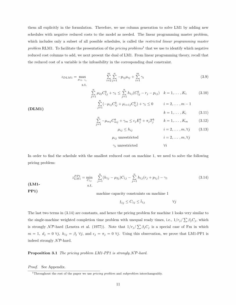
them all explicitly in the formulation. Therefore, we use column generation to solve LM1 by adding new

schedules with negative reduced costs to the model as needed. The linear programming master problem,

which includes only a subset of all possible schedules, is called the restricted linear programming master

problem RLM1. To facilitate the presentation of the pricing problems1 that we use to identify which negative

reduced cost columns to add, we next present the dual of LM1. From linear programming theory, recall that

the reduced cost of a variable is the infeasibility in the corresponding dual constraint.

(DLM1)

zDLM1 = maxµij, γi

m∑i=2

n∑j=1

−pijµij +m∑

i=1

γi (3.9)

s.t.n∑

j=1

µ2jCk1j + γ1 ≤

n∑j=1

h1j(Ck1j − rj − p1j) k = 1, . . . , K1 (3.10)

n∑j=1

(−µijCkij + µi+1jC

kij) + γi ≤ 0 i = 2, . . . , m− 1

k = 1, . . . , Ki (3.11)n∑

j=1

−µmjCkmj + γm ≤ εjE

kj + πjT

kj k = 1, . . . , Km (3.12)

µij ≤ hij i = 2, . . . , m,∀j (3.13)

µij unrestricted i = 2, . . . , m,∀j

γi unrestricted ∀i

In order to find the schedule with the smallest reduced cost on machine 1, we need to solve the following

pricing problem:

(LM1-

PP1)

zPP1LM1 = min

C1j

n∑j=1

(h1j − µ2j)C1j −n∑

j=1

h1j(rj + p1j)− γ1 (3.14)

s.t.

machine capacity constraints on machine 1

t1j ≤ C1j ≤ t1j ∀j

The last two terms in (3.14) are constants, and hence the pricing problem for machine 1 looks very similar to

the single-machine weighted completion time problem with unequal ready times, i.e., 1/rj/∑

βjCj , which

is strongly NP-hard (Lenstra et al. (1977)). Note that 1/rj/∑

βjCj is a special case of Fm in which

m = 1, dj = 0 ∀j, h1j = βj ∀j, and εj = πj = 0 ∀j. Using this observation, we prove that LM1-PP1 is

indeed strongly NP-hard.

Proposition 3.1 The pricing problem LM1-PP1 is strongly NP-hard.

Proof. See Appendix.1Throughout the rest of the paper we use pricing problem and subproblem interchangeably.

11

Similarly, all pricing problems on machines 2 through m − 1 are weighted completion time problems with

unequal ready times; the objective function coefficients have a different structure than (3.14), however, as

shown below.

(LM1-

PPi)

zPPiLM1 = min

Cij

n∑j=1

(µij − µi+1j)Cij − γi (3.15)

s.t.

machine capacity constraints on machine i

tij ≤ Cij ≤ tij ∀j

The pricing problem on the last machine, presented below, has a similar structure to the single-machine

weighted earliness/tardiness problem with unequal ready times, i.e., 1/rj/∑

(εjEj + πjTj). The latter is

strongly NP-hard which follows from the complexity of 1/rj/∑

πjTj (Lenstra et al. (1977)) which is a

special case of 1/rj/∑

(εjEj + πjTj).

(LM1-

PPm)

zPPmLM1 = min

Cmj

n∑j=1

[(εj − µmj)Ej + (πj + µmj)Tj ] +n∑

j=1

µmjdj − γm (3.16)

s.t.

machine capacity constraints on machine m

tmj ≤ Cmj ≤ tmj ∀j

By recognizing that 1/rj/∑

(εjEj + πjTj) is a special case of Fm in which m = 1, and h1j = 0 ∀j, it can be

proved that LM1-PPm is strongly NP-hard. We omit the proof which is very similar to that of Proposition

3.1.

Proposition 3.2 The pricing problem LM1-PPm is strongly NP-hard.

Finally, observe that 1/rj/∑

βjCj is also a special case of 1/rj/∑

(εjEj +πjTj) obtained by setting all due

dates equal to zero (dj = 0, ∀j), and all tardiness costs equal to the completion time costs (πj = βj , ∀j).

This allows us, by setting the problem parameters appropriately, to use the heuristics developed by Bulbul

et al. (2001) for 1/rj/∑

(εjEj +πjTj) to solve all pricing problems approximately. In Section 4.1, we explain

in greater detail how we solve these single-machine subproblems.

Corresponding Lagrangian Problem

An alternate decomposition approach is Lagrangian relaxation. For a given set of dual variables {µij}, the

Lagrangian function LR1(µij) is obtained from Fm by dualizing the operation precedence constraints (2.4).

In fact, LM1 is equivalent to the Lagrangian dual problem LD1 which maximizes LR1(µij) presented below

over the dual variables (Lagrange multipliers). See Wolsey (1998) for a discussion of the duality between

DW reformulation and Lagrangian relaxation.

12

(LR1(µij))

zLR1(µij) = minCij , wij

n∑j=1

(h1j − µ2j)C1j −n∑

j=1

h1j(rj + p1j) (3.17)

+m−1∑i=2

n∑j=1

(µij − µi+1j)Cij (3.18)

+n∑

j=1

[(εj − µmj)Ej + (πj + µmj)Tj ] +n∑

j=1

µmjdj (3.19)

+m∑

i=2

n∑j=1

(hij − µij)wij (3.20)

−m∑

i=2

n∑j=1

pijµij (3.21)

s.t.

(2.3), (2.5)-(2.8)

µij unrestricted i = 2, . . . , m, ∀j (3.22)

By comparing (3.14) with (3.17), (3.15) with (3.18), and (3.16) with (3.19), we note that the Lagrangian

subproblems are the same as the pricing problems of LM1 except for the dual variables associated with

the convexity constraints (3.5) which are constants in the pricing problems. Therefore, if there exists a

procedure to update the Lagrange multipliers that is computationally less expensive than solving a linear

program, then we can potentially solve LD1 more quickly than LM1. Unfortunately, we cannot apply

subgradient optimization to update the dual variables because we are not guaranteed to find a subgradient

in each iteration. Recall that some of the subproblems are strongly NP-hard and we solve all subproblems

approximately. Hence, we do not attempt to solve LD1, but use LR1(µij) to compute an alternate lower

bound on the objective function value of the optimal integer solution for a given set of dual variables {µij}.

As we discuss in Sections 3.4 and 4.1, in certain cases this improves the overall performance of our algorithm

significantly.

Second DW Reformulation

Our objective is to find a near-optimal feasible solution for the original integer programming problem Fm

by using information from the solution of a relaxation of the problem. Thus, it is important not only that

the lower bound be tight, but also that the solution itself be easily modified into a near-optimal feasible

solution. However, optimal solutions for LM1 have a property that does not generally hold for optimal

integer solutions:

Lemma 3.3 There exists an optimal solution to LM1 such that w∗ij = 0, i = 2, . . . ,m, ∀j.

Proof. See Appendix.

In the lemma above and throughout the rest of the paper, an asterisk denotes the optimal value of a

variable. Furthermore, in Lemma 3.8 we show that for an important special inventory cost structure, all

13

optimal solutions of LM1 have this property. We also note that in LM1, the waiting time variables do not

appear in the pricing problems. Thus, in an optimal solution for LM1, the inventory holding costs are not

necessarily reflected either by the waiting time variables or by the schedules we generate. Consequently, we

expect that LM1 will produce solutions that are poor starting points for constructing near-optimal feasible

solutions; for this reason we consider an alternate DW reformulation. However, we include LM1 here because

the computational experiments do not always reflect our expectations.

In the new formulation, we incorporate the effect of the waiting times implicitly in the objective function

coefficients of the schedules identified by the column generation procedure, and consequently in the pricing

problems as well. By substituting wij = Cij − Ci−1j − pij we obtain an alternate DW reformulation:

(IM2)

zIM2 = minxk

i

K1∑k=1

[n∑

j=1

(h1j − h2j)Ck1j − h1j(rj + p1j)

]xk

1 (3.23)

+m−1∑i=2

Ki∑k=1

[n∑

j=1

(hij − hi+1j)Ckij

]xk

i (3.24)

+Km∑k=1

[n∑

j=1

((εj − hmj)Ek

j + (πj + hmj)T kj

)]xk

m (3.25)

+n∑

j=1

hmjdj −m∑

i=2

n∑j=1

hijpij (3.26)

s.t.

(µij)Ki−1∑k=1

Cki−1jx

ki−1 −

Ki∑k=1

Ckijx

ki ≤ −pij i = 2, . . . , m, ∀j (3.27)

(γi)Ki∑k=1

xki = 1 i = 1, . . . , m (3.28)

xki ∈ {0, 1} i = 1, . . . , m

k = 1, . . . , Ki (3.29)

Relaxing the integrality constraints (3.29) yields the (restricted) linear programming master problem LM2

(RLM2). The pricing problems of LM2 differ from those of LM1 only in their objective functions. (See Table

1 below.)

Corresponding Lagrangian Problem

The corresponding Lagrangian dual problem of LM2, which we call LD2, maximizes LR2(µij) over the

nonnegative dual variables µij . We omit the formulation of LR2(µij) because it is structurally very similar

to that of LR1(µij). However, note that in IM2 the operation precedence constraints (3.27) must be modeled

as inequalities because the waiting time variables are dropped from the formulation. Therefore, the dual

variables in LR2 are not unrestricted. (Compare to (3.22) in LR1.)

Table 1 summarizes the subproblems for the models discussed in this section. For each subproblem type,

the first row is the objective function to be minimized on a single machine over the appropriate set of feasible

14

schedules, and the second row is an associated additive constant, given the problem parameters and a set of

dual variables.

With Waiting Time Vars. Without Waiting Time Vars.

(LM1/LR1) (LM2/LR2)

DW LR DW LR

PP1n∑

j=1

(h1j − µ2j)C1j Samen∑

j=1

(h1j − h2j − µ2j)C1j Same

−n∑

j=1

h1j(rj + p1j)− γ1 −n∑

j=1

h1j(rj + p1j) * *

PPi†n∑

j=1

(µij − µi+1j)Cij Samen∑

j=1

(hij − hi+1j + µij − µi+1j)Cij Same

−γi 0 * *

PPmn∑

j=1

[(εj − µmj)Ej + (πj + µmj)Tj ] Samen∑

j=1

[(εj − hmj − µmj)Ej + (πj + hmj + µmj)Tj ] Same

n∑j=1

µmjdj − γm

n∑j=1

µmjdj * *

(†)For i = 2, . . . , m− 1.

(∗)Same as their counterparts in models with waiting time variables.

Table 1: Summary of subproblems.

Pricing Problem Objectives

The key to solving LM1 and LM2 effectively is to understand the nature of the pricing problems. Note that

there is no explicit reason why the objective function coefficients of the completion time or the tardiness

variables in the pricing problems must be nonnegative. Below, we give an interpretation of the pricing

problem objectives and discuss the implications if there exist completion time or tardiness variables with

negative objective function coefficients in the pricing problems. First, in order to simplify the discussion, we

introduce the term “t-boundedness”:

Definition 3.4 In a pricing problem, if at least one tardiness variable Tj or a completion time variable Cij

has a negative objective function coefficient, then this pricing problem is called t-bounded. Otherwise, it is

called bounded.

Observe that a completion time/tardiness variable with a negative objective function coefficient in the pricing

problem of machine i would imply that we could identify schedules with arbitrarily small reduced costs if the

minimization were not carried out over a polytope of feasible schedules, i.e., Si. However, Cij ≤ tij holds in

all pricing problems, which motivates the definition above.

Now, we explain the interplay between the inventory holding costs and the dual variables for job j on

machine i (2 ≤ i ≤ m− 1) using (3.30)-(3.31):

15

Ki−1∑k=1

Cki−1jx

ki−1 −

Ki∑k=1

Ckijx

ki = −pij (3.30)

Ki∑k=1

Ckijx

ki −

Ki+1∑k=1

Cki+1jx

ki+1 = −pi+1j (3.31)

where we assume that strict complementary slackness holds, i.e., µij < 0 and µi+1j < 0. Note that (3.30)-

(3.31) belong to the set of constraints (3.27) with the slack variables equal to zero. A similar analysis can be

carried out for the other pricing problems as well. Assume that we increase Cij by a small amount δ > 0 while

keeping Ci−1j and Ci+1j constant. Then, the marginal increase in cost for job j is (hij −hi+1j)δ. In order to

measure the effect induced on other jobs we use the “shadow price” interpretation of dual variables and view

this change in Cij as an equivalent decrease/increase in the right hand side of (3.30)/(3.31). The resulting

marginal increase in the objective function is given by µij(−δ) + µi+1jδ = (−µij + µi+1j)δ, for sufficiently

small δ. Thus, we observe that the objective function coefficient of Cij in LM2-PPi, i = 2, . . . , m− 1, is the

difference between these two effects, i.e., (hij − hi+1j)− (−µij + µi+1j), and the sign of this difference is not

necessarily nonnegative.

This potential “t-boundedness” in the pricing problems has very significant practical implications. Al-

though we can solve the t-bounded pricing problems as effectively as we can the bounded pricing problems

(see Section 4.1), t-boundedness has several negative consequences. First, we observe that when some pricing

problems are t-bounded, other bounded pricing problems generally do not yield negatively priced schedules,

and the column generation algorithm converges very slowly. Second, t-boundedness may cause the column

generation algorithm to terminate prematurely with a large optimality gap as we demonstrate in our com-

putational study. Third, the performance of the simplex algorithm suffers while solving the LP master

problems, and each iteration of the column generation algorithm takes longer due to t-boundedness. Note

that the columns from the t-bounded pricing problems that are added to the LP master problems may have

coefficients that are much larger than those of other columns. Consequently, the LP master problem becomes

poorly scaled, and numerical difficulties appear in the simplex algorithm.

3.2 Models With Artificial Variables

In this section, we develop conditions for boundedness of all pricing problem objectives and introduce a two-

phase approach for solving LM1 and LM2 using these conditions and LP duality theory. As we demonstrate

in our computational study, this approach speeds up the convergence of the column generation algorithm

significantly.

Lemma 3.5 In LM1, all pricing problems are bounded if the dual variables µij (i = 2, . . . , m, ∀j) satisfy

16

the following relationships:

µ2j ≤ h1j ∀j (3.32)

−µij + µi+1j ≤ 0 i = 2, . . . ,m− 1, ∀j (3.33)

−µmj ≤ πj ∀j (3.34)

In LM2, all pricing problems are bounded if the dual variables µij (i = 2, . . . , m, ∀j) satisfy the following

relationships:

µ2j ≤ h1j − h2j ∀j (3.35)

−µij + µi+1j ≤ hij − hi+1j i = 2, . . . ,m− 1, ∀j (3.36)

−µmj ≤ πj + hmj ∀j (3.37)

Proof. These conditions follow from nonnegativity of the objective function coefficients of the completion

time and tardiness variables in the pricing problems.

Furthermore, by constraint (3.13) of DLM1, all dual variables of LM1 satisfy:

µij ≤ hij i = 2, . . . ,m, ∀j, (3.38)

and from (3.27) the following holds for the dual variables of LM2:

µij ≤ 0 i = 2, . . . ,m, ∀j. (3.39)

Together, these observations lead us to the lemma below:

Lemma 3.6 For all optimal solutions of LM1:

µ∗ij ≤ min1≤k≤i

hkj i = 2, . . . ,m, ∀j (3.40)

For all optimal solutions of LM2:

µ∗ij ≤ min(0, h1j − hij) i = 2, . . . ,m, ∀j (3.41)

Proof. See Appendix.

Lemma 3.6 provides some economic insight into our problem as well. Suppose that we obtain an optimal

solution to LM1 and would like to know how the objective function would change if we reduce the processing

time of job j on machine i by one time unit. Clearly, we can keep the current schedule and incur hij for

the additional delay between machine i − 1 and machine i. However, this lemma tells us that there may

17

be better alternatives. The reduction in pij can also be viewed as an increase in the right hand side of the

corresponding operation precedence constraint. Hence, the marginal change in the optimal cost is µ∗ij and

bounded by min1≤k≤i

hkj , which implies that the slack introduced between the operations of job j on machines

i− 1 and i can be absorbed anywhere upstream from machine i.

Below, we prove a stronger version of Lemma 3.3 after defining an important economic concept for our

problem. Note that each operation on a job consumes resources (e.g., materials, labor), adding value to the

product. Hence, one can often assume that the inventory holding cost of a job is increasing as it proceeds

through its processing stages, which motivates the following definition:

Definition 3.7 The m-machine flow shop is said to be a value-added chain if the inventory holding costs

are strictly increasing over the processing stages, i.e., h1j < h2j < · · · < hmj < εj , ∀j.

Our algorithms do not make any specific assumption about the cost structure; however, part of our

computational study will be devoted to exploring the effect of the assumption of a “value-added chain” on

the performance of our algorithms because it reflects a commonly observed relationship among holding costs.

Furthermore, the lemma below provides additional motivation to compare LM1 and LM2.

Lemma 3.8 If the m-machine flow shop is a value-added chain, then in all optimal solutions of LM1,

w∗ij = 0, i = 2, . . . ,m, ∀j.

Proof. See Appendix.

Now, we are ready to introduce our two-phase approach to solve LM1 and LM2 in which we impose a

structure on the dual variables according to Lemmas 3.5 and 3.6. Observe that this structure is automatically

satisfied by the optimal dual variables of LM1 and LM2, but not necessarily by the optimal dual variables of

the restricted LP master problems RLM1 and RLM2. Our approach is based on the correspondence of dual

constraints and primal variables which implies that in order to impose a constraint on the dual variables we

need to introduce primal variables.

In the first phase, we add artificial primal variables into the LP master problems that constrain the dual

variables in such a way that the pricing problems are always bounded. The intent is to generate schedules

that drive the solutions of the restricted LP master problems RLM1/RLM2 towards the optimal solutions

of LM1/LM2, and we stop when we cannot identify any negatively priced schedules. However, when we

terminate the column generation algorithm in this phase, there is no guarantee that all artificial variables

will be equal to zero because in the first phase we solve a related but a slightly different problem.

In the second phase, we drive the artificial variables to zero using complementary slackness. We gradually

relax the constraints that we impose in the first phase by increasing the objective function coefficients of

18

the artificial variables. Note that during this phase it is quite possible that some of the pricing problems

become t-bounded. We terminate the column generation when all artificial variables are equal to zero and

we cannot find any negatively priced columns. Overall, this approach enables us to avoid t-bounded pricing

problems initially, speeds up the convergence of the column generation, and reduces the optimality gap.

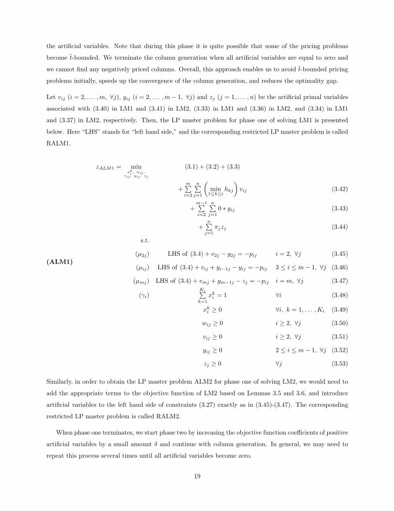
Let vij (i = 2, . . . , m, ∀j), yij (i = 2, . . . , m− 1, ∀j) and zj (j = 1, . . . , n) be the artificial primal variables

associated with (3.40) in LM1 and (3.41) in LM2, (3.33) in LM1 and (3.36) in LM2, and (3.34) in LM1

and (3.37) in LM2, respectively. Then, the LP master problem for phase one of solving LM1 is presented

below. Here “LHS” stands for “left hand side,” and the corresponding restricted LP master problem is called

RALM1.

(ALM1)

zALM1 = minxk

i, wij,

vij , yij , zj

(3.1) + (3.2) + (3.3)

+m∑

i=2

n∑j=1

(min

1≤k≤ihkj

)vij (3.42)

+m−1∑i=2

n∑j=1

0 ∗ yij (3.43)

+n∑

j=1

πjzj (3.44)

s.t.

(µ2j) LHS of (3.4) + v2j − y2j = −pij i = 2, ∀j (3.45)

(µij) LHS of (3.4) + vij + yi−1j − yij = −pij 3 ≤ i ≤ m− 1, ∀j (3.46)

(µmj) LHS of (3.4) + vmj + ym−1j − zj = −pij i = m, ∀j (3.47)

(γi)Ki∑k=1

xki = 1 ∀i (3.48)

xki ≥ 0 ∀i, k = 1, . . . , Ki (3.49)

wij ≥ 0 i ≥ 2, ∀j (3.50)

vij ≥ 0 i ≥ 2, ∀j (3.51)

yij ≥ 0 2 ≤ i ≤ m− 1, ∀j (3.52)

zj ≥ 0 ∀j (3.53)

Similarly, in order to obtain the LP master problem ALM2 for phase one of solving LM2, we would need to

add the appropriate terms to the objective function of LM2 based on Lemmas 3.5 and 3.6, and introduce

artificial variables to the left hand side of constraints (3.27) exactly as in (3.45)-(3.47). The corresponding

restricted LP master problem is called RALM2.

When phase one terminates, we start phase two by increasing the objective function coefficients of positive

artificial variables by a small amount δ and continue with column generation. In general, we may need to

repeat this process several times until all artificial variables become zero.

19

The advantage of this two-phase approach derives from the fact that although LM1 differs from ALM1,

and LM2 differs from ALM2, the corresponding pricing problems have exactly the same structure. Thus, we

are able to impose a structure on the dual variables without the need for new algorithms for the pricing prob-

lems. Some stronger results can be obtained from the Lagrangian relaxations ALR1/ALR2 corresponding

to ALM1/ALM2:

(ALR1(µij))

zALR1(µij) = minCij, wij

vij , yij , zj

(3.17) + (3.18) + (3.19) + (3.20) + (3.21)

+m∑

i=2

n∑j=1

(min

1≤k≤ihkj − µij

)vij (3.54)

+m−1∑i=2

n∑j=1

(µij − µi+1j)yij (3.55)

+n∑

j=1

(πj + µmj)zj (3.56)

s.t.

(2.3), (2.5)-(2.8)

(3.22)

(3.51)− (3.53)

Observe that ALR1(µij) and LR1(µij) are identical, except for the terms (3.54)-(3.56) in the objective

function of ALR1(µij) that are based on Lemmas 3.5 and 3.6. ALR2(µij) can be obtained from LR2(µij) in

a similar way. Then, the Lagrangian dual problems ALD1 and ALD2 maximize ALR1(µij) and ALR2(µij)

over the dual variables, respectively. The Lagrangian functions with artificial variables have an additional

advantage over their corresponding DW reformulations; not only are their subproblems the same as those of

their counterparts with no artificial variables, but there is also no need for a “phase two” in the Lagrangian

case as we prove next.

Lemma 3.9 There exist optimal solutions to ALD1 and ALD2 such that v∗ij = 0 (i = 2, . . . , m, ∀j),

y∗ij = 0 (i = 2, . . . , m− 1, ∀j) and z∗j = 0 (j = 1, . . . , n).

Proof. The proof is similar to that of Lemma 3.3. See Appendix.

Now, we are ready to present our main result in this section:

Proposition 3.10 All linear programming master problems and Lagrangian dual problems presented in Sec-

tion 3 have the same optimal objective function value, i.e.,

zLM1 = zLM2 = zLD1 = zLD2 = zALM1 = zALM2 = zALD1 = zALD2 (3.57)

20

Proof. Clearly, zLM1 = zLM2. Then, zLM1 = zLD1, zLM2 = zLD2, zALM1 = zALD1 and zALM2 = zALD2

follow from the equivalence of corresponding DW reformulations and Lagrangian dual problems. By Lemma

3.9, we have zLD1 = zALD1 and zLD2 = zALD2 which establishes the desired result.

In summary, all models we consider have the same optimal objective function value; however, their optimal

solutions have different properties, which has very significant practical consequences, as we demonstrate in

our computational study. Also, although the objective function coefficients may have a different structure

from pricing problem to pricing problem, we always solve weighted completion time problems on machines

1 through m− 1 and an earliness/tardiness problem on the last machine.

Finally, in the proposition below we establish the relationship between the optimal objective function

values of our models and the optimal objective function value of the LP relaxation of TIFm.

Proposition 3.11 The optimal objective function value of LM1 is greater than or equal to that of the LP

relaxation of TIFm, i.e., zLPTIFm ≤ zLM1.

Proof. See Appendix.

In other words, our models can provide tighter bounds on the optimal integer solution than the LP

relaxation of TIFm. In addition, our models have shorter solution times than that of the LP relaxation of

TIFm, especially for large problem instances. (See Section 5.)

3.3 Switching From Column Generation to Lagrangian Relaxation

Although we do not solve any Lagrangian dual problem explicitly, we use the Lagrangian functions to

compute alternate lower bounds, both on the optimal objective value of the LP master problems and on the

optimal integer objective value.

The link between the LP master problems and the Lagrangian functions is established through dual vari-

ables, i.e., we can pass the optimal dual variables of the restricted LP master problems to the corresponding

Lagrangian functions and compute alternate lower bounds. Recall that the conditions in Lemmas 3.5 and

3.6 are not necessarily satisfied by the optimal dual variables of a restricted LP master problem. However,

here Lagrangian relaxation has one advantage over column generation: in column generation, the values of

the dual variables are dictated by a linear program whereas we are able to manipulate the dual variables

before optimizing the Lagrangian function. Thus, in any iteration of the column generation algorithm, we

can take the optimal dual vector of the restricted LP master problem, change the values of the dual variables

according to Algorithm 1 for RLM1/RALM1 and Algorithm 2 for RLM2/RALM2 (see below), and then

minimize the corresponding Lagrangian function with this new dual vector. Algorithms 1 and 2 ensure that

the dual variables passed to Lagrangian relaxation satisfy the conditions in Lemmas 3.5 and 3.6. In addition,

21

in the computational experiments, we observed that after running these algorithms, the dual variables differ

very little from their original values.

Lemma 3.12 For any optimal dual vector {µij} from RLM1/RALM1 (RLM2/RALM2), the dual variables

satisfy the conditions in Lemmas 3.5 and 3.6 when Algorithm 1 (Algorithm 2) terminates.

Proof. See Appendix.

Algorithm 1 Adjusting Dual Variables For RLM1/RALM1Require: An optimal dual vector {µij} for the restricted LP master problem RLM1 or RALM1 is given.

1: µij = max(−πj , µij), i = 2, . . . , m, ∀j

2: µij = min(hij , µij), i = 2, . . . , m, ∀j

3: µ2j = min(h1j , µ2j), ∀j

4: for j = 1 to n do

5: for i = 2 to m− 1 do

6: µi+1j = min(µij , µi+1j)

Algorithm 2 Adjusting Dual Variables For RLM2/RALM2Require: An optimal dual vector {µij} for the restricted LP master problem RLM2 or RALM2 is given.

1: µij = max(−πj − hij , µij), i = 2, . . . , m, ∀j

2: µ2j = min(0, h1j − h2j , µ2j), ∀j

3: for j = 1 to n do

4: for i = 2 to m− 1 do

5: µi+1j = min(0, µij + hij − hi+1j , µi+1j)

3.4 Lower Bounds and Feasible Integer Solutions

Lower Bounds

A well known drawback of column generation algorithms is that although a good solution is usually obtained

quickly it may take a very long time to prove LP optimality. See Barnhart et al. (1998) for a discussion of

this so-called “tailing-off effect.”

This problem is particularly relevant to our case because we are not even guaranteed to find the LP

optimal solution, as some of our pricing problems are strongly NP-hard, and all pricing problems are solved

heuristically. Therefore, in order to terminate the column generation procedure when a good, but not

necessarily optimal solution is found, we need a tight lower bound on the optimal objective value of the

LP master problem. Of course, such a lower bound can also be used to quantify the optimality gap of the

22

feasible integer solutions we construct. Bounds based on the optimal objective value of the current restricted

LP master problem and the objective values of the pricing problems appear in Lasdon (1970), Farley (1990)

and Vanderbeck and Wolsey (1996). We follow a similar approach.

From LP duality theory, we know that the objective value of any dual feasible solution provides a lower

bound on the optimal objective value of the primal problem, and that the reduced cost of a variable is the

infeasibility in the corresponding dual constraint. These two facts together imply that we can construct a

dual feasible solution using the optimal objective values of the pricing problems (reduced costs), and thus

compute a lower bound on the optimal objective value of the LP master problem. Below, we develop a lower

bound on the optimal objective value of LM1, and analogous lower bounds can be computed for the other LP

master problems. In the following discussion, a bar under an optimal objective value denotes a corresponding

lower bound. Let {µij , γi} represent the optimal dual variables of RLM1 in the current iteration. Then,

{µij , γ′i} is a feasible solution for DLM1, where

γ′i = γi + zPPiLM1, ∀i. (3.58)

To see why this holds, observe that adding the optimal objective values from the pricing problems to

the dual variables associated with the convexity constraints decreases the left hand sides of constraints

(3.10)-(3.12) in DLM1, exactly by the amount of infeasibility. Thus, {µij , γ′i} is feasible for DLM1, and

zLM1 =m∑

i=2

n∑j=1

−pijµij +m∑

i=1

γ′i (3.59)

is a lower bound on zLM1 and the optimal integer solution. The only modification necessary for our problem

is to replace zPPiLM1 by zPPi

LM1 in (3.58) because we solve the pricing problems approximately. In order to

compute the lower bounds zPPiLM1 ∀i, we use the algorithms developed by Bulbul et al. (2001) who provide a

tight lower bound for the single-machine earliness/tardiness scheduling problem.

A similar lower bound can be obtained from Lagrangian relaxation as well. Note that zLR1(µij) =m∑

i=1

zPPiLM1 +

m∑i=1

γi−m∑

i=2

n∑j=1

pijµij where the last two terms are constant for a given set of dual variables. Thus,

similar to above,

zLR1(µij) =m∑

i=1

zPPiLM1 +

m∑i=1

γi −m∑

i=2

n∑j=1

pijµij (3.60)

is a lower bound on zLM1 and zIM1. Together with the algorithms in Section 3.3 to pass dual vectors from

column generation to Lagrangian relaxation, (3.60) provides a very useful alternate lower bound for our

problem.

23

Feasible Integer Solutions

In order to construct feasible solutions for the original integer programming problem Fm, we need a job

processing sequence on each machine. Then, given these sequences we can solve TTFm (see Section 2), and

obtain a feasible integer solution for the original problem. In general, TTFm is a small LP that is solved

optimally very quickly. Hence, the major concern here is to find good job processing sequences, which we

obtain in two different ways.

First, for all jobs and all machines, we compute the completion time of job j on machine i in the optimal

solution of the current restricted LP master problem as:

C ′ij =

K′i∑

k=1

Ckijx

ki , (3.61)

assuming that there are K ′i columns for machine i in the current restricted LP master problem. Then,

we generate job processing sequences on each machine by sequencing jobs in non-decreasing order of these

completion times. Finally, we find the optimal schedule given these sequences by solving TTFm which yields

a feasible solution for Fm.

Second, for each machine i, we identify the schedule Ski with the largest xk

i value in the current solution,

and use the sequence of that schedule in solving TTFm. Similarly, we obtain job processing sequences from

the heuristic solutions of Lagrangian subproblems, and construct feasible integer solutions.

4 Column Generation

In this section, we briefly discuss some details of the column generation algorithm and then summarize our

approach to solve the single-machine subproblems.

Creating An Initial Feasible Restricted LP Master Problem

Creating a good feasible initial restricted LP master problem is important to ensure that proper dual infor-

mation is passed to the pricing problems. In order to start the column generation procedure with a good

set of columns, we initially assign values to the dual variables such that the conditions in Lemmas 3.5 and

3.6 are satisfied (see below). Then, we solve the pricing problems with these dual variables, obtain job

processing sequences from their solutions, and timetable these sequences with TTFm to obtain a feasible

integer solution. Clearly, adding the individual machine schedules from this feasible integer solution to the

restricted LP master problem guarantees a feasible LP solution. The dual variables are initialized as:

24

µij = min1≤k≤i

hkj i = 2, . . . , m, ∀j. (For RLM1/RALM1) (4.1)

µij = min1≤k≤i

hkj − hij i = 2, . . . , m, ∀j. (For RLM2/RALM2) (4.2)

Lemma 4.1 The dual variables in (4.1) and (4.2) satisfy the conditions in Lemmas 3.5 and 3.6.

Proof. See Appendix.

Adding Columns

Our heuristics to solve the single-machine subproblems may identify several different negatively priced

columns in a single iteration. (See Section 4.1.) However, our preliminary computational results indicated

that although this approach may allow the column generation procedure to terminate in fewer iterations, the

total CPU time is generally much longer because the size of the restricted LP master problem grows very

rapidly and each iteration consumes substantially more time. Therefore, in each iteration we add at most

one column from each subproblem.

In Lemma 3.3, we established that there exists an optimal solution to LM1 such that all waiting times

are equal to zero. Motivated by this lemma, whenever we identify a negatively priced schedule on machine

i to be added to RLM1/RALM1, we generate schedules on all machines using Algorithm 3 such that no job

waits between its operations, and add these schedules to the restricted LP master problem as well. These

no-wait schedules do not necessarily have negative reduced costs, and we may delete them later. However,

our initial results indicated that this approach speeds up the convergence and decreases the total CPU time

of the column generation procedure for solving LM1/ALM1 considerably despite the rapid growth of the

restricted LP master problems.

Algorithm 3 Generating No-Wait Schedules For RLM1/RALM1

Require: A negatively priced schedule Ski on machine i is given.

1: for q = i to m− 1 do

2: Ckq+1j = Ck

qj + pq+1j , ∀j {No job waits between its operations}

3: for q = i downto 2 do

4: Ckq−1j = Ck

qj − pqj , ∀j {No job waits between its operations}

5: for j = 1 to n− 1 do {Assume jobs are in sequence order}

6: for i = 1 to m do

7: if Ckij > Ck

ij+1 − pij+1 then {Machine capacity is violated}

8: Shift all operations of job j + 1 forward by Ckij − Ck

ij+1 + pij+1

9: Add schedules Sk1 , . . . , Sk

m to RLM1/RALM1.

25

In order to speed up the column generation procedure further, we apply a local improvement algorithm

to existing columns in order to identify new schedules with negative reduced costs. (See Algorithm 4 below.)

One major advantage of the local improvement algorithm is that it is much faster than solving the pricing

problems and potentially decreases the total number of iterations. For each machine i, a good starting

schedule for the local improvement algorithm is the column with the largest xki value in the current solution.

If we can improve on such a schedule, we may intuitively expect that it would enter the solution with a

larger xki value, increasing the quality of our feasible integer solutions. Note that large xk

i values imply that

the optimal solution of the current restricted LP master problem is close to integral (see (3.61)), and we

may expect that the feasible integer solutions obtained from the optimal solution of the current restricted

LP master problem have small optimality gaps. (See Section 3.4.) Our computational study demonstrates

that the local improvement scheme is extremely useful, in accordance with the observations of Savelsbergh

and Sol (1998) for a different problem.

Algorithm 4 Local Improvement On Existing ColumnsRequire: An initial schedule Sk

i on machine i.

1: for j = 1 to n− 1 do {Assume jobs are in sequence order}

2: Reverse the sequence of jobs j and j + 1.

3: Schedule j + 1 and j optimally in the interval [Ckij − pij , Ck

ij+1].

4: if the sequence j + 1, j does not decrease the reduced cost of Ski then

5: Recover the original schedule before the interchange

6: STOP if no improvement during an entire pass through Ski , otherwise go back to Step 1.

Removing Columns

Column deletion is an essential part of our column management strategy. We observed that the columns

that are added at the initial stages of the column generation procedure are usually not present in the final

solution. This is particularly true for LM1/LM2, and if we never remove any columns, then solving the

restricted LP master problem becomes eventually very time consuming. Therefore, we delete columns by

using a rule similar to that in Van den Akker et al. (2002). Let zFm and zFm represent the best lower

bound and the best integer solution available for the original scheduling problem, respectively. Then, we

delete columns with a reduced cost strictly larger than zFm−zFm because they cannot appear in an optimal

integer solution. Clearly, these columns may be necessary for solving the LP master problems, in which case

they will be generated again.

Here, we need to re-emphasize the significance of Lagrangian relaxation in obtaining an alternate lower

bound. It potentially improves the best lower bound available, and thus increases the number of columns

deleted and speeds up the column generation algorithm. In fact, we always perform one Lagrangian iteration

before any column deletion step.

26

Termination Conditions

For large problems, generating columns until we cannot identify any negatively priced column may take a

very long time, with no significant improvement in the objective function value of the restricted LP master

problem or the feasible integer solution. Therefore, we compute various quantities and terminate column

generation when one of them is sufficiently small.

Ideally, we would like to stop when the integer optimality gap (zFm − zFm)/zFm is small enough, but

unfortunately, this gap is usually quite large and does not provide useful information. As an alternative,

we terminate column generation when (zRLM − zLM )/zLM or (zRLM − zLR(µij))/zLR(µij) is sufficiently

small, where zRLM is the optimal objective function value of the current restricted LP master problem,

and zLR(µij) is the objective function value of the (not necessarily optimal) solution of the corresponding

Lagrangian relaxation LR(µij). The latter ratio does not have any theoretical meaning; however, it is a useful

stopping condition for hard problems in which the other gaps are not within specified limits. Note that the

optimal objective of LR(µij) is a lower bound on the optimal objective of the LP master problem, and the

gap between zRLM and zLR(µij) still provides a good stopping condition when the others fail. Occasionally,

we continue generating columns with no decrease in the objective function value of the restricted LP master

problem, indicating degeneracy in the simplex algorithm. In those cases, we stop if the objective does not

improve in n consecutive iterations.

4.1 Subproblems

We use the heuristics developed by Bulbul et al. (2001) for the single-machine earliness/tardiness scheduling

problem to solve all subproblems. Note that a weighted completion time problem is a special case of an

earliness/tardiness problem with all due dates set equal to zero, and the tardiness costs set equal to the

completion time costs. Thus, we are able to solve all subproblems within a unified framework. Below, we

explain the fundamental ideas behind our single-machine heuristics and then discuss briefly the modifications

that arise from negative earliness or tardiness costs in the subproblem objectives.

To solve the single-machine earliness/tardiness (E/T) problem P1, we follow a two-phase approach,

where in the first phase we obtain a good job processing sequence, and in the second phase we schedule

jobs optimally given the job sequence. Our approach incorporates computing a fast and tight preemptive

lower bound for P1, and using information from the lower bound solution to construct near-optimal feasible

schedules for P1. To compute the preemptive lower bound, we divide the jobs into unit time intervals and

construct a transportation problem TR1 by assigning a cost to each of these unit jobs and considering an

appropriate planning horizon which depends on the ready times, due dates and the sum of the processing

times. In general, TR1 corresponding to a weighted completion time problem is solved more quickly than

TR1 corresponding to an E/T problem because weighted completion time problems have shorter planning

27

horizons than E/T problems. The cost structure of the unit jobs is fundamental to the success of our

algorithms, and when all earliness and tardiness costs are positive, all unit jobs of a job are within a single

block in the optimal solution of TR1, where a block is a sequence of unit jobs processed without idle time.

(See Kanet and Sridharan (2000) for a discussion of the well known block structure in the E/T problems.) We

observe that in these blocks, less expensive jobs are split more, and more expensive jobs are scheduled almost

contiguously and close to their positions in the optimal non-preemptive schedule. Based on this observation,

we construct various job processing sequences that yield excellent non-preemptive feasible schedules for P1.

From Section 3.1, we know that depending on the relative values of inventory holding and tardiness costs

and dual variables, some jobs may have negative earliness or tardiness costs in the subproblem objectives. In

this case, we need two types of modifications to our single-machine algorithms. First, the planning horizon

needs to be expanded to account for negative costs if we want to compute a lower bound from TR1. However,

in our column generation algorithm, we compute the planning horizon only once at the beginning under the

assumption of positive costs because we do not want to lose speed by increasing the size of the subproblems.

Thus, we give up our ability to compute lower bounds from column generation in favor of solution speed, if

there are negative costs. Note that we can still obtain lower bounds from Lagrangian relaxation, if there are

no negative earliness costs, by using the approach in Section 3.3 that removes all negative completion time

and tardiness costs in Lagrangian subproblem objectives. This is particularly important when solving LM1

and LM2, in which the pricing problems are t-bounded until the solution gets close to optimality.

Second, we need to ensure that jobs whose tardiness costs are negative appear at the end of the job

processing sequence for single-machine timetabling. To achieve this, we solve TR1 with a planning horizon

determined under the assumption of positive earliness and tardiness costs, generate job processing sequences,

and then transfer jobs with negative tardiness costs to the end of the sequence. Afterwards, when we solve the

single-machine timetabling LP for machine i, which is obtained from TTFm by setting m = 1, the simplex

algorithm identifies a feasible schedule Sk−1i and an unboundedness ray λi if there are negative tardiness costs.

Thus, the completion times in the final single-machine schedule Ski are computed as Ck

ij = Ck−1ij +αλij where

λij is the jth component of λi and α = minπj<0tij−Ck−1

ij

λij.

Finally, we need to mention that if there are t-bounded subproblems, we only solve these for a few

iterations of the column generation algorithm and skip the bounded subproblems. This enhancement is

based on the observation that if there exist t-bounded subproblems, usually no negatively priced columns

are identified by solving the bounded subproblems.

28

5 Computational Experiments

We performed a variety of computational experiments in order to evaluate the performance of both the lower

bounds and the feasible integer solutions. The experimental design has two main objectives. First, we would

like to demonstrate that our algorithms find good solutions and find them rapidly. There are two important

factors that affect the speed of our algorithms: the size of the restricted LP master problem, which depends

on the number of columns added, and the sizes of the subproblems, where the sum of the processing times

on machine i determines the size of the subproblem corresponding to machine i.

Our other major concern is the robustness of our algorithms. In particular, we are interested in the

performance of our algorithms as the number of machines, the number of jobs and the length of the processing

times increase. The importance of the latter derives from the fact that we use a preemptive relaxation when

solving the single-machine subproblems (see Section 4.1), and the number of preemptions increases as the

processing times increase. The cost structure is also potentially important because t-boundedness is related

to the relative magnitudes of the costs and the dual variables.

Finally, we compare the performance of our algorithms to that of the LP relaxation of TIFm. Recall that

in Proposition 3.11 we proved that zLM1 is a tighter bound on the optimal integer solution than is zLPTIFm.

Here, we demonstrate that our column generation procedure is also faster than solving the LP relaxation of

TIFm, especially for large problem instances. Additionally, it provides a good starting point for constructing

near-optimal feasible integer solutions while there is no obvious way of converting the solution of the LP

relaxation of TIFm into a feasible integer solution.

5.1 Data Generation

On each machine i, the processing times are generated from a discrete uniform distribution U [pi, pi]. Then,

the ready times are generated from a discrete uniform distribution U [0, b0.5P1c], where P1 =∑n

j=1 p1j .

In scheduling problems with due dates, it is widely observed that the tightness and range of the due dates

play an important role in determining the level of difficulty. (See Potts and van Wassenhove (1982) and Hall

and Posner (2001).) Therefore, in setting the due dates, we follow a scheme similar to those of Pinedo and

Singer (1999) and Eilon and Chowdhury (1976), where we change the due date tightness systematically. The

due date of job j is set equal to brj + fdj

∑mi=1 pijc, where fd

j is the due date slack factor of job j and is

generated from a continuous uniform distribution U [TF − RDD2 , TF + RDD

2 ]. TF is the mean due date

slack factor, and RDD is the range of the due date slack factors.

The inventory holding costs {h1j} are generated from a uniform distribution U [1, 50]. Then, hij =

fcijhi−1j (i = 2, . . . , m), εj = fc

m+1hmj and πj = fcm+2εj , where fc

ij is a percentage generated from a

29

continuous uniform distribution U [fc

ij, f

c

ij ]. This method enables us to model different cost structures

easily.

5.2 Summary of Results

Our algorithms were implemented in C using the CPLEX 7.0 callable libraries. For benchmarking, TIFm

and/or its linear programming relaxation were solved via ILOG AMPL/CPLEX 7.0. All computations were

performed on a Sun UltraSPARC-IIi 440MHz computer with 256 MB of memory.

In the following sections, we discuss the designs and results of the various experiments we conducted to

explore the solution quality and/or time of our algorithms. Specifically, we examine the effects of the number

of machines and jobs, the length of the processing times and the cost structure.

5.2.1 Number of Machines and Jobs

In order to test how increasing the number of machines and/or the number of jobs affects the CPU time and

the solution quality of our algorithms, we design experiments with the parameters given in Table 2. The

due date slack factor, TF , has three different levels for each m, corresponding to tight, moderately tight and

loose due dates. In order to maintain approximately the same percentage of tardy jobs across different m for

a given TF level, we need to increase the numerical value of TF as m increases due to increasing queueing

effects when there are more machines. For each combination of parameters, 5 instances are generated,

resulting in a total of 15 problems for each combination of m and n. When possible, the problems are solved

optimally using the time-indexed formulation TIFm. However, for instances in which AMPL/CPLEX identifies

at least one feasible integer solution but cannot verify optimality within a maximum CPU time of half an

hour, we report the best integer solution obtained. The CPU time of the branch-and-bound algorithm for

solving TIFm optimally is limited to half an hour because our goal here is to demonstrate that our algorithms

consistently yield high quality feasible schedules to the original problem in a short period of time compared

to an alternate method. As explained below, for large problem instances, it is often difficult to even find a

single feasible solution for TIFm in half an hour of CPU time.

m n pij , ∀i TF RDD fcij/100, i = 2, . . . , m + 1 fc

m+2j/100

2 {10, 20, 30} U[1, 10] {1.5, 2.5, 3.5} 0.4 U[1.0, 1.5] U[1.5, 2.0]

3 {10, 20, 30} U[1, 10] {2.0, 3.0, 4.0} 0.4 U[1.0, 1.5] U[1.5, 2.0]

4 {10, 20, 30} U[1, 10] {2.5, 3.5, 4.5} 0.4 U[1.0, 1.5] U[1.5, 2.0]

Table 2: Effect of the Number of Machines and Jobs: Problem Parameters.

In Tables 5 and 6, we report the performance of our lower bounds and heuristics as the number of

30

machines and jobs increase, both in terms of solution quality and solution time. The columns #OP (“Number

Optimal”) and #BI (“Number Best Integer”) indicate the number of times AMPL/CPLEX terminated with the

optimal integer and a feasible integer solution without verifying optimality within the time limit, respectively.

For example, for m = 4 and n = 10, AMPL/CPLEX found the optimal integer solution for TIFm in 1 instance,

terminated with a feasible integer solution in 7 instances, and could not identify any integer solution for the

remaining 7 instances in half an hour of CPU time. Our preliminary computational tests for m ≥ 3 and n ≥ 20

indicated that AMPL/CPLEX could generally not find any feasible integer solution in half an hour of CPU time.

Therefore, we do not report any integer results from AMPL/CPLEX for problems with n ≥ 20, except for m = 2.

This is indicated by N/A (“Not Available”) in columns #OP and #BI. For any LP master problem LM, the

columns LB (“Lower Bound”) and MA-LP (“Master-Linear Programming”) indicate the optimality gap of

the restricted LP master problem, when column generation terminates, with respect to our lower bound (LB)

and the lower bound from the LP relaxation of TIFm (MA-LP), respectively. Specifically, LB = zRLM−zLM

zLM∗

100%, and MA − LP = zRLM−zLP T IF m

zLP T IF m∗ 100%. In order to quantify the quality of our feasible integer

solutions, we report zF m−zLP T IF m

zLP T IF m∗ 100% in the column IF-LP (“Integer Feasible-Linear Programming”)

which is an upper bound on the optimality gap of our feasible integer solutions. In addition, the column IF-

AP (“Integer Feasible-AMPL”) compares our feasible integer solutions to the optimal or best integer solutions

obtained from AMPL/CPLEX. A minus sign in column IF-AP indicates that our integer solutions are superior

to those obtained from AMPL/CPLEX. Under the CPU times, the column MA (“Master”) is the total CPU

time of the column generation algorithm in seconds, and MA/LP (“Master/Linear Programming”) is the

ratio of the solution time of our algorithm to that of the LP relaxation of TIFm. In each cell, the first number

is the performance measure when no local improvement in column generation is invoked, and the number

in parentheses is the corresponding measure when we perform local improvement on existing columns to

identify negatively priced columns. For each value of n, the first row indicates the average and the second

row indicates the worst case performance.

From Tables 5 and 6, it is clear that generating columns by local improvement makes a substantial

difference, both in terms of percentage gaps and solution time. In particular, note that LM1 performs poorly

in some instances, e.g., for m = 2 and n = 30, if no local improvement is carried out in column generation.

The average and worst case optimality gaps of our lower bound decrease as the number of machines

increases. For a given m, these gaps may increase or decrease as the number of jobs increases; however,

they are relatively close to each other. Overall, as the problem size increases, the quality of our lower bound

improves. Note that for ALM2, m = 4, and n = 30, the average and worst case optimality gaps of our lower

bound are 4.57% and 9.99%, respectively, when local improvement is invoked. We note that LM1 has the

worst lower bound performance; the other three are similar.

Similar qualitative observations hold for the optimality gap of the LP master problems. The gap MA-LP

decreases as the number of machines increases, but the number of jobs does not have an important impact

31

on the optimality gap of the LP master problems for a given m. We note that although ALM1, LM2 and

ALM2 yield similar results, the performance of LM1 is poor when we do not perform local improvement.

In this case, local improvement or the introduction of artificial variables (ALM1) has a tremendous positive

effect. For ALM1, LM2, and ALM2, the average gaps are within 2% and the worst case gaps are within 5%,

with or without local improvement, when m = 4 and n = 30. Note that by Proposition 3.11, these are upper

bounds on the gaps, and we re-emphasize that approximate solutions for the subproblems have a significant

speed advantage, and compromise very little in solution quality.

For very small problems, AMPL/CPLEX outperforms our algorithms in obtaining feasible integer solutions.

Note that for the 14 instances solved to optimality by AMPL/CPLEX where m = 2 and n = 10, the average gap

between the objective of the feasible integer solutions obtained by LM1/LM2 (with local improvement) and

that from AMPL/CPLEX (IF-AP) is approximately 6-7%. For m ≥ 3, the feasible integer solutions identified

by our algorithms are significantly superior to those of AMPL/CPLEX. For 8 instances with m = 4 and n = 10

for which AMPL/CPLEX was able to return an integer solution after half an hour of CPU time, LM1 and

LM2 find feasible integer solutions within 1 second that are on average 43% better. We also note that the

optimality gaps of our feasible integer solutions with respect to the LP relaxation of TIFm (IF-LP) increase

as the problem size grows. This may be because the LP relaxation of TIFm becomes looser as the problem

size increases.

There is a trade-off between solution speed and quality of the feasible integer solutions. Comparing LM1

with ALM1 and LM2 with ALM2 shows that the solution speed gained from the use of artificial variables

comes at the expense of the quality of feasible integer solutions. When solving ALM1 and ALM2, many

fewer columns are added, which implies that there is less information available to construct job processing

sequences for feasible integer solutions, and thus the sequences are more likely to contain errors. In Section

3.1, we argue that LM1 may not be a good starting point for constructing feasible integer solutions because

of Lemma 3.3; however, the results indicate the contrary. ALM2 has in general the shortest CPU times, and

the worst integer solutions.

Even if we were only interested in finding good lower bounds to the original flow shop scheduling problem

Fm, our algorithms, with their short CPU times and small optimality gaps, would be superior to solving

the LP relaxation of TIFm. Note that ALM2 with local improvement is almost 5 times faster than the LP

relaxation of TIFm when m = 4 and provides solutions that are on average within 1.16% of optimality across

45 instances. In general, our strategy to avoid t-boundedness initially and then drive artificial variables to

zero serves very well in obtaining excellent LP solutions. It provides stability, i.e., smaller worst case bounds,

and speed.

Finally, although we do not report detailed results here, we observe that the due date tightness has

an important impact on problem difficulty. Under tight due dates, the gaps LB, MA-LP and the solution

32

times increase, however the quality of the feasible integer solutions appears not to be sensitive to due date

tightness.

5.2.2 Processing Times

We also investigate whether our algorithms are sensitive to increases in processing times, which may imply a

potential increase in the number of preemptions when solving the subproblems, and thus adversely affect the

solution quality. The problem parameters for our experiments are given in Table 3. For each combination of

parameters, 5 instances are generated, resulting in a total of 15 problems for each combination of m and n.

Note that the problems with pij ∼ U [1, 10] are the same problems as in the previous section. In this section,

we do not report the column IF-AP because AMPL/CPLEX is unable to find feasible integer solutions when the

processing times increase. In all problems reported in Table 7, local improvement is invoked during column

generation.

m n pij , ∀i TF RDD fcij/100, i = 2, . . . , m + 1 fc

m+2j/100

2 {10, 20} U[1, 10], U[1, 20], U[1, 30] {1.5, 2.5, 3.5} 0.4 U[1.0, 1.5] U[1.5, 2.0]

3 {10, 20} U[1, 10], U[1, 20], U[1, 30] {2.0, 3.0, 4.0} 0.4 U[1.0, 1.5] U[1.5, 2.0]

Table 3: Effect of Processing Times: Problem Parameters.

The robustness of our approach is evident from the results in Table 7. As the processing times increase,

there is sometimes a slight degradation in the performance measures LB and MA-LP, although this effect

is less pronounced than the effect of an increase in the number of machines and jobs. The combined effect

of increasing the number of machines and jobs and the length of the processing times is a decrease in the

percentage gaps of LB and MA-LP. In general, the quality of our lower bound does not seem to be jeopardized

by the larger number of preemptions that occurs when processing times are longer. For all models, when

m = 3, n = 20, and pij ∼ U [1, 30], the average gap of our lower bound (LB) ranges from 8.7 to 10.91% and

the average gap of our LP master problems (MA-LP) ranges from 2.40 to 2.56%, respectively. The effect of

the processing times on the optimality gap of the feasible integer solutions is not consistent; in some cases

it is positive, in others, negative. However, this effect is clearly not as significant as the effect of the number

of machines and jobs.

The size of our subproblems depends on the sum of the processing times(Bulbul et al. (2001)). Therefore,

we expect the solution time for the subproblems to increase with the processing times, and Table 7 verifies

this trend. However, we observe that the CPU time of our algorithms is much less sensitive to the planning

horizon than the LP relaxation of TIFm. When m = 3, n = 20, and pij ∼ U [1, 30], our algorithms are

5.5-12.5 times faster than the LP relaxation of TIFm.

33

5.2.3 Cost Structure

In order to explore the sensitivity of our algorithms to the inventory holding cost structure, we compare the

performance of our algorithms for problems with non-decreasing inventory holding costs in Section 5.2.1 to

the performance when fcij/100 ∼ U [0.8, 1.2] (i = 2, . . . , m + 1), i.e., the inventory holding costs are similar.

All other parameters are the same as in Section 5.2.1.

We do not report detailed results here, but make the following observations: whether the inventory holding

costs satisfy the value-added assumption or are similar to each other, we obtain good lower bounds and high

quality feasible integer solutions. We note that we have slightly better feasible integer solutions when costs

are similar, and attribute this to the fact that “errors” in the job processing sequences are potentially more

costly when inventory costs are non-decreasing. Also, despite Lemma 3.8, the integer solutions obtained from

LM1 are in general better than those from LM2 for problems with non-decreasing inventory holding costs.

The solution times are insensitive to the cost structure as well, except for the largest problems. For those

instances (m = 3, n = 30), problems with similar inventory holding costs appear to be easier to solve. We

conclude that in general, the cost structure does not affect the performance of our algorithms significantly.

5.2.4 Permutation Sequences

Finally, we report some observations regarding the structure of the job processing sequences that can be of

great value for future research. Recall that we do not require a permutation sequence, i.e., the sequence of

jobs may differ from one machine to another, and our algorithms yield high quality feasible integer solutions.

Therefore, if we can show that the job processing sequences we generate do not deviate significantly from

a permutation sequence, there is motivation to devise algorithms that construct permutation sequences

exclusively in search for a good solution. This would reduce the number of possible job processing sequences

to consider from O((n!)m) to O(n!), possibly allowing us to design more effective algorithms. Now, let

qj = 1m

∑mi=1 |sj − sij | represent the permutation index of job j, where sij is the sequence number of job

j in the job processing sequence of machine i, and sj is the average sequence number of job j across all

machine sequences. This is therefore a measure of deviation from a permutation sequence for job j. Then,

we define the permutation index of our problem to be: q = 1n

∑nj=1 qj . We would expect q to be equal to

zero if we have a permutation sequence, hence the lower is q, the closer are our job processing sequences to

a permutation sequence. The average and the standard deviation of the permutation indices for a subset of

problems from the previous section are given in Table 4. Each statistic is computed across 15 instances.

From Table 4, we note that when the inventory holding costs are non-decreasing over the processing

stages, our job processing sequences are very close to permutation sequences. However, when inventory

holding costs are similar, the job processing sequences deviate more from a permutation sequence because

the trade-offs among operations of different jobs are less significant. The results in Table 4 indicate that

34

there may be advantages to solution methods that focus on permutation sequences.

m = 2, n = 10 m = 3, n = 10

Non-decreasing Costs Similar Costs Non-decreasing Costs Similar Costs

Average 0.16 0.21 0.08 0.56

Standard Deviation 0.21 0.23 0.09 0.34

Table 4: Permutation Indices.

6 Concluding Remarks

We developed a method to solve the m-machine flow shop scheduling problem with intermediate inventory

holding, earliness and tardiness costs. This model is one of the first to incorporate work-in-process inventory

holding costs in scheduling, and was partly motivated by recent examples from the biotechnology industry

where work-in-process is expensive and needs special treatment while waiting for processing at the next

stage.

We use mathematical programming methods to solve our problem. We reformulate the problem with an

exponential number of variables, solve its LP relaxation approximately by column generation, and develop

simple and effective ways of obtaining feasible solutions to the original problem. We exploit the duality

between Dantzig-Wolfe reformulation and Lagrangian relaxation extensively to develop structural properties

and tune our models accordingly. To the best of our knowledge, this paper is the first attempt to apply column

generation to a machine scheduling problem in which some of the subproblems are strongly NP-hard. Our

computational study demonstrates that heuristic solutions for the subproblems provide a significant speed

advantage over alternate methods and do not compromise solution quality.

We recognize that our model has several limitations. We assume complete knowledge of all parameters

of all jobs to arrive in the future, but this is rarely true in real life settings. However, it is customary to

schedule the available jobs using available information, so the problem still needs to be solved. We also note

that we cannot accommodate precedence constraints among jobs on the same machine as it would destroy

the structure of the subproblems. Nevertheless, we are encouraged by the performance of our algorithms,

and as a more general setting, we hope to develop approaches for the job shop scheduling problem with

intermediate inventory holding, earliness and tardiness costs.

Acknowledgment

We would like to thank Professor Alper Atamturk for his helpful insights. We also would like to thank

the associate editor and the anonymous referees for their valuable comments. This research was partially

supported by NSF Grant DMI-0092854.

35

AMPL/CPLEX

Percentage

Gap

(†)

CP

UT

ime

(sec.)

(†)

mn

#O

P#

BI

LM

1A

LM

1LM

1A

LM

1

LB

MA

-LP

IF-L

PIF

-AP

LB

MA

-LP

IF-L

PIF

-AP

MA

MA

/LP

MA

MA

/LP

210

14

121.1

5(17.2

7)

3.8

9(2.6

2)

26.3

6(18.9

3)

12.0

5(5.7

7)

18.1

4(20.0

4)3.5

5(2.5

2)

27.6

1(24.5

9)

12.8

9(10.5

8)

0.3

7(0.2

5)

1.1

9(0.8

0)

0.2

4(0.2

3)

0.7

6(0.7

1)

107.8

2(5

7.6

8)

26.4

9(1

1.5

6)

68.8

2(5

5.0

4)

33.5

9(1

4.9

1)

61.4

4(7

4.8

2)

16.6

0(1

4.5

6)

87.8

1(7

1.6

0)

33.3

6(4

8.0

4)

0.6

0(0

.39)

2.0

0(1

.39)

0.4

1(0

.68)

1.1

4(1

.36)

20

09(∗∗)

18.0

5(16.0

9)

5.4

6(3.3

1)

40.9

1(37.2

7)-4

7.7

3(-4

7.5

3)15.7

8(13.7

1)4.0

0(3.1

5)

49.8

7(41.5

5)-4

6.4

4(-4

7.4

0)

3.6

7(2.2

5)

1.4

0(0.8

7)

2.3

1(1.2

9)

0.8

9(0.4

9)

52.6

8(4

5.3

8)

11.1

4(7

.27)

71.7

5(8

6.3

5)

-0.8

8(6

.40)

51.1

4(3

8.6

4)

10.5

3(8

.31)

127.9

9(1

16.9

5)

-1.1

9(-

1.1

9)

5.4

9(3

.33)

2.3

0(1

.39)

4.4

1(2

.21)

1.6

8(0

.97)

30

N/A

N/A

1302.2

5(11.9

9)(∗)

44.7

4(2.9

3)

40.5

7(30.5

0)

N/A

13.3

4(12.3

2)4.2

6(3.2

0)

40.8

7(42.3

7)

N/A

14.6

7(10.9

9)1.1

7(0.8

8)11.2

0(6.8

0)0.9

0(0.5

4)

15457.1

0(2

0.1

0)

163.4

9(5

.54)

80.5

4(4

7.7

2)

N/A

21.0

8(2

0.0

6)

7.1

4(5

.45)

83.1

4(9

7.3

2)

N/A

24.5

9(2

0.7

9)

2.1

9(1

.89)

35.5

0(1

8.7

0)

2.9

6(1

.42)

310

312

5.4

0(6.4

0)

1.6

6(1.2

9)

16.7

2(18.0

5)-1

9.1

7(-1

8.2

0)

5.9

6(5.7

8)

1.7

7(1.2

5)

28.3

5(22.9

2)-1

0.3

1(-1

4.0

4)

0.4

5(0.3

4)

0.6

4(0.5

0)

0.2

3(0.2

2)

0.3

3(0.3

3)

23.8

3(2

3.5

6)

9.0

8(8

.65)

55.4

2(6

2.1

7)

2.7

8(1

1.4

7)

26.9

8(2

6.1

9)

10.6

2(8

.28)

67.3

9(5

8.5

6)

26.8

8(2

2.6

2)

1.1

2(0

.91)

1.2

3(1

.05)

0.6

3(0

.43)

0.6

4(0

.66)

20

N/A

N/A

7.5

4(8.3

1)(∗)

37.6

7(1.6

1)

57.5

6(51.1

6)

N/A

8.5

4(7.7

6)

1.9

9(1.4

3)

69.1

1(63.6

6)

N/A

8.3

4(5.6

5)

1.1

9(0.8

0)

5.0

1(2.8

0)

0.6

1(0.3

6)

18.1

1(2

1.2

0)

351.2

5(3

.49)

242.8

1(1

15.3

6)

N/A

23.3

4(1

8.0

4)

5.4

9(4

.00)

174.4

9(1

42.5

4)

N/A

19.5

9(1

0.4

1)

2.3

0(1

.55)

16.7

0(1

2.1

3)

1.9

6(1

.21)

30

N/A

N/A

8.0

3(8.7

9)(∗)

127.3

4(26.2

4)86.3

7(66.0

9)

N/A

11.2

7(9.3

6)

3.0

5(2.3

8)

70.6

8(79.3

3)

N/A

59.7

9(43.0

1)1.6

0(1.0

7)51.1

4(19.8

7)1.3

3(0.5

0)

13.4

9(1

9.8

6)

407.1

6(3

61.6

3)

224.3

7(1

56.5

3)

N/A

25.6

3(2

0.7

9)

5.6

0(4

.40)

133.0

8(1

47.8

8)

N/A

142.2

2(1

05.6

4)

4.1

8(2

.46)

110.1

9(4

4.5

4)

3.2

4(1

.04)

410

17(∗∗)

2.1

6(2.0

9)

0.3

3(0.2

7)

14.5

6(13.9

0)-4

3.2

6(-4

3.1

5)

1.9

6(2.0

1)

0.2

9(0.3

1)

32.4

7(30.5

4)-2

9.8

8(-2

9.7

2)

0.3

8(0.3

3)

0.3

7(0.3

2)

0.2

3(0.2

4)

0.2

3(0.2

3)

5.6

5(5

.38)

1.1

5(1

.09)

66.4

7(6

6.4

7)

0.1

5(0

.15)

4.6

0(5

.50)

1.0

9(1

.30)

86.7

9(7

9.3

9)

15.0

1(1

5.0

1)

0.9

9(0

.79)

1.0

3(0

.81)

0.5

5(0

.50)

0.5

7(0

.52)

20

N/A

N/A

4.9

6(5.5

2)(∗)

61.6

2(2.0

5)

56.7

1(49.0

2)

N/A

6.5

5(5.4

2)

2.3

3(1.9

0)

77.5

8(80.2

6)

N/A

14.9

4(12.5

5)1.0

1(0.8

3)

8.3

9(3.6

6)

0.5

6(0.2

5)

13.6

8(1

2.4

4)

399.6

9(4

.95)

217.5

0(1

37.4

0)

N/A

21.1

4(1

9.8

5)

5.9

5(5

.30)

161.9

4(2

17.5

0)

N/A

54.7

7(3

4.4

1)

3.1

9(2

.29)

35.9

9(1

1.4

6)

2.4

0(0

.72)

30

N/A

N/A

5.1

7(6.1

7)(∗)

222.1

5(1.6

4)106.1

2(64.4

5)

N/A

6.2

5(5.9

2)

1.7

9(1.4

9)99.5

0(105.6

2)

N/A

44.3

4(88.6

5)0.6

3(1.1

6)85.0

1(33.4

7)1.1

0(0.4

3)

9.8

7(1

4.5

1)

475.7

1(3

.31)

211.6

9(1

62.9

1)

N/A

12.3

5(1

3.1

9)

3.6

2(2

.30)

146.7

3(1

83.3

7)

N/A

304.1

1(1

73.0

1)

3.5

0(2

.10)

294.6

2(9

5.7

0)

4.2

1(1

.22)

(†)

Ineach

cell,th

enum

ber

outs

ide

(insi

de)

the

pare

nth

ese

sis

the

measu

rew

ithout

(wit

h)

localim

pro

vem

ent.

For

each

n,th

e1st

(2nd)

row

indic

ate

sth

eavera

ge

(wors

tcase

)perf

orm

ance.

(∗)

Negati

ve

low

er

bounds

from

pro

ble

ms

wit

hno

localim

pro

vem

ent

not

inclu

ded

inth

era

tio.

The

actu

alavera

ge

gap

acro

ss15

inst

ances

ishig

her.

(∗∗)

Inth

isro

w,IF

-AP

iscom

pute

dacro

ssin

stances

for

whic

ha

feasi

ble

solu

tion

exis

ts.

Tab

le5:

Effe

ctof

the

Num

ber

ofM

achi

nes

and

Jobs

:A

vera

gean

dW

orst

Cas

eG

aps

ofH

euri

stic

san

dB

ound

s,C

PU

Tim

es.

36

AMPL/CPLEX

Percentage

Gap

(†)

CP

UT

ime

(sec.)

(†)

mn

#O

P#

BI

LM

2A

LM

2LM

2A

LM

2

LB

MA

-LP

IF-L

PIF

-AP

LB

MA

-LP

IF-L

PIF

-AP

MA

MA

/LP

MA

MA

/LP

210

14

116.5

9(19.8

8)3.1

1(2.8

1)

21.6

8(20.5

8)

8.1

7(7.1

4)

18.0

1(16.1

5)3.9

3(2.1

9)

28.2

6(25.6

1)

13.7

9(11.1

3)

0.3

9(0.2

2)

1.3

0(0.7

0)

0.3

7(0.2

0)

1.1

7(0.6

4)

53.2

3(8

2.1

8)

13.5

0(1

4.4

0)

62.1

3(5

7.1

0)

24.7

1(1

7.0

1)

98.1

5(5

1.7

8)

26.6

8(1

0.5

9)

68.8

2(8

6.0

3)

34.3

3(2

6.9

0)

0.6

5(0

.39)

2.5

0(1

.03)

1.7

4(0

.32)

5.6

1(1

.04)

20

09(∗∗)22.9

3(17.1

5)5.4

9(3.5

2)

44.3

5(45.4

6)-4

4.5

8(-4

3.6

1)15.1

1(13.7

9)5.6

4(4.1

1)

55.0

1(51.2

0)

-36.3

9(-4

2.6

8)

3.6

4(2.0

3)

1.3

7(0.7

7)

1.8

3(1.3

6)

0.7

2(0.5

8)

110.0

9(5

8.3

5)

14.9

1(9

.67)

106.7

9(8

3.0

0)

14.2

3(7

.63)

30.1

7(3

3.3

9)

17.7

3(1

4.5

2)

137.1

1(1

31.4

8)

49.4

6(2

8.5

8)

4.9

5(2

.68)

2.1

9(1

.28)

3.3

4(3

.30)

1.9

0(2

.20)

30

N/A

N/A

14.2

4(12.3

5)4.3

9(3.0

1)

40.2

7(33.4

0)

N/A

12.8

7(10.7

5)4.3

3(3.0

3)

42.0

1(43.7

5)

N/A

16.9

8(9.2

0)

1.3

5(0.7

3)

8.7

5(8.3

2)

0.7

1(0.6

6)

25.5

5(2

0.3

4)

8.5

8(7

.96)

86.3

8(5

3.3

7)

N/A

23.4

4(2

4.2

8)

8.8

5(5

.72)

76.0

6(1

07.3

1)

N/A

22.1

8(1

5.4

4)

1.9

7(1

.38)

22.4

0(2

6.4

0)

1.8

7(1

.89)

310

312

4.9

1(5.3

6)

1.5

0(1.6

5)

17.9

4(18.5

7)-1

8.1

4(-1

7.4

9)

4.4

4(4.3

5)

1.3

7(1.2

7)

60.0

4(43.2

1)

13.9

2(3.8

7)

0.5

5(0.3

9)

0.8

1(0.5

8)

0.2

7(0.2

3)

0.3

9(0.3

4)

18.6

7(2

1.5

1)

9.0

2(8

.28)

56.1

7(5

8.7

1)

3.0

3(7

.99)

18.6

3(2

1.5

1)

8.6

7(8

.28)

208.4

3(1

31.3

4)

199.8

7(1

03.1

9)

1.2

5(0

.71)

1.4

8(1

.03)

0.7

2(0

.48)

1.1

1(0

.74)

20

N/A

N/A

9.1

2(8.7

2)

2.1

5(1.7

0)

48.7

7(52.6

4)

N/A

8.2

4(8.0

9)

1.9

6(1.4

0)

120.6

3(65.7

0)

N/A

8.3

5(4.7

0)

1.1

6(0.6

5)

4.0

1(2.2

2)

0.5

0(0.2

9)

22.5

2(1

8.9

8)

5.3

8(3

.74)

119.8

5(1

21.3

5)

N/A

19.5

6(2

3.2

8)

4.4

8(3

.76)

289.1

6(1

56.2

6)

N/A

17.2

1(8

.13)

2.0

2(0

.96)

14.5

8(5

.56)

1.7

2(0

.56)

30

N/A

N/A

11.4

0(9.4

2)

3.0

7(2.1

9)

59.3

5(59.5

2)

N/A

8.6

3(8.6

6)

2.8

9(2.0

8)

89.5

8(90.4

0)

N/A

52.6

5(39.9

5)1.3

3(0.9

9)28.4

6(14.6

8)0.7

1(0.3

7)

29.2

5(2

1.3

5)

6.2

3(4

.75)

93.8

9(9

3.7

7)

N/A

16.1

9(2

0.7

8)

4.8

8(3

.40)

316.8

4(1

85.2

7)

N/A

88.5

6(1

19.9

9)

2.6

0(2

.55)

75.7

7(3

0.8

8)

1.8

5(0

.75)

410

17(∗∗)

2.1

1(2.0

4)

0.2

9(0.3

3)

14.7

2(12.9

9)-4

3.3

0(-4

2.9

4)

1.9

9(1.9

8)

0.3

2(0.3

2)

92.4

5(107.2

7)-1

8.0

0(-1

7.0

9)

0.6

3(0.5

0)

0.6

1(0.4

8)

0.2

1(0.2

1)

0.2

0(0.2

1)

4.9

9(4

.86)

1.4

6(1

.86)

92.3

5(5

8.2

1)

0.1

5(0

.15)

4.6

3(4

.70)

1.1

8(1

.18)

196.4

7(4

09.2

1)

35.5

9(4

5.9

3)

1.2

0(1

.11)

1.2

5(1

.16)

0.4

3(0

.46)

0.4

5(0

.48)

20

N/A

N/A

6.7

5(5.7

1)

2.4

7(2.1

1)

46.3

0(49.1

3)

N/A

5.1

1(4.5

4)

2.4

8(1.8

6)

159.1

9(86.0

9)

N/A

13.9

6(9.3

7)

1.0

1(0.6

6)

5.4

8(3.3

8)

0.3

7(0.2

3)

21.0

3(1

5.6

8)

5.8

9(7

.64)

125.2

1(1

46.0

0)

N/A

14.7

2(1

2.8

5)

9.8

3(6

.42)

399.8

0(2

18.5

8)

N/A

31.3

8(1

6.5

3)

2.0

9(1

.01)

16.6

2(8

.16)

1.0

4(0

.43)

30

N/A

N/A

6.5

9(6.7

0)

1.9

1(1.5

7)

63.0

4(67.2

5)

N/A

5.4

1(4.5

7)

1.8

0(1.3

1)226.6

7(154.7

3)

N/A

96.0

1(69.4

4)1.3

1(0.9

5)39.5

4(14.6

1)0.5

1(0.1

9)

12.2

1(1

8.8

3)

3.4

9(4

.25)

159.7

5(1

64.3

0)

N/A

11.2

9(9

.99)

4.3

1(2

.21)

781.2

6(5

10.7

4)

N/A

143.8

8(1

11.7

2)

1.9

5(1

.68)

110.8

2(4

0.2

5)

1.5

4(0

.52)

(†)

Ineach

cell,th

enum

ber

outs

ide

(insi

de)

the

pare

nth

ese

sis

the

measu

rew

ithout

(wit

h)

localim

pro

vem

ent.

For

each

n,th

e1st

(2nd)

row

indic

ate

sth

eavera

ge

(wors

tcase

)perf

orm

ance.

(∗∗)

Inth

isro

w,IF

-AP

iscom

pute

dacro

ssin

stances

for

whic

ha

feasi

ble

solu

tion

exis

ts.

Tab

le6:

Effe

ctof

the

Num

ber

ofM

achi

nes

and

Jobs

:A

vera

gean

dW

orst

Cas

eG

aps

ofH

euri

stic

san

dB

ound

s,C

PU

Tim

es.

37

Percentage

Gap

(†)

CP

UT

ime

(sec.)

(†)

mn

pij,∀i

LM

1A

LM

1LM

2A

LM

2LM

1A

LM

1LM

2A

LM

2

LB

MA

-LP

IF-L

PLB

MA

-LP

IF-L

PLB

MA

-LP

IF-L

PLB

MA

-LP

IF-L

PM

AM

A/LP

MA

MA

/LP

MA

MA

/LP

MA

MA

/LP

210

U[1

,10]

17.2

72.6

218.9

320.0

42.5

224.5

919.8

82.8

120.5

816.1

52.1

925.6

10.2

50.8

00.2

30.7

10.2

20.7

00.2

00.6

4

57.6

811.5

655.0

474.8

214.5

671.6

082.1

814.4

057.1

051.7

810.5

986.0

30.3

91.3

90.6

81.3

60.3

91.0

30.3

21.0

4

U[1

,20]

19.0

33.7

219.7

112.2

13.2

627.9

618.7

65.2

424.7

510.7

52.9

124.1

10.2

80.3

10.2

10.2

30.2

90.3

30.3

30.3

1

79.2

913.9

077.7

436.5

410.7

981.0

371.5

625.7

089.9

137.8

311.9

161.8

40.4

50.5

50.3

70.4

20.5

60.7

41.9

71.4

1

U[1

,30]

22.3

95.9

023.3

622.5

03.7

026.6

621.4

83.7

821.0

320.0

83.2

126.4

40.3

80.2

00.2

90.1

50.3

90.1

90.3

40.1

7

69.9

530.5

780.4

970.5

320.1

985.8

672.9

119.6

480.5

087.5

715.1

784.2

10.7

00.3

80.5

00.2

50.6

60.3

30.8

10.3

9

20

U[1

,10]

16.0

93.3

137.2

713.7

13.1

541.5

517.1

53.5

245.4

613.7

94.1

151.2

02.2

50.8

71.2

90.4

92.0

30.7

71.3

60.5

8

45.3

87.2

786.3

538.6

48.3

1116.9

558.3

59.6

783.0

033.3

914.5

2131.4

83.3

31.3

92.2

10.9

72.6

81.2

83.3

02.2

0

U[1

,20]

18.6

44.3

746.2

617.6

14.1

549.0

219.9

75.1

439.9

015.6

84.2

547.6

83.4

90.3

02.0

20.1

93.0

80.2

72.2

20.1

9

55.5

311.5

186.3

862.7

013.5

5105.6

370.2

814.4

259.7

151.7

612.2

8111.0

14.7

00.4

73.2

60.5

25.3

10.5

44.1

20.3

7

U[1

,30]

19.5

94.4

336.1

118.8

25.2

249.7

520.3

14.8

236.3

716.5

24.6

152.5

04.5

50.1

93.2

30.1

44.2

00.1

72.5

60.1

1

37.1

39.4

855.8

438.2

714.2

387.4

057.0

411.9

759.1

333.7

513.2

5144.6

65.8

80.2

67.0

20.2

85.7

70.2

35.2

40.3

3

310

U[1

,10]

6.4

01.2

918.0

55.7

81.2

522.9

25.3

61.6

518.5

74.3

51.2

743.2

10.3

40.5

00.2

20.3

30.3

90.5

80.2

30.3

4

23.5

68.6

562.1

726.1

98.2

858.5

621.5

18.2

858.7

121.5

18.2

8131.3

40.9

11.0

50.4

30.6

60.7

11.0

30.4

80.7

4

U[1

,20]

7.9

11.5

231.0

17.8

21.7

047.7

47.9

51.8

237.0

07.2

51.9

967.4

50.4

50.2

20.3

40.1

70.5

00.2

30.3

20.1

5

54.9

812.0

799.3

553.1

615.6

7135.1

453.5

316.4

8142.8

948.0

119.5

5234.1

21.0

10.5

70.5

50.3

21.2

80.4

70.6

30.2

8

U[1

,30]

8.6

41.0

933.9

96.7

70.7

444.6

57.7

71.0

630.7

37.0

11.0

191.3

70.5

30.0

90.3

90.0

70.6

40.1

20.3

80.0

7

51.2

05.0

0173.1

128.0

52.3

3154.3

137.5

45.0

3111.5

536.6

74.7

1232.7

71.1

30.2

00.8

60.1

01.3

00.1

90.7

70.1

0

20

U[1

,10]

8.3

11.6

151.1

67.7

61.4

363.6

68.7

21.7

052.6

48.0

91.4

065.7

05.6

50.8

02.8

00.3

64.7

00.6

52.2

20.2

9

21.2

03.4

9115.3

618.0

44.0

0142.5

418.9

83.7

4121.3

523.2

83.7

6156.2

610.4

11.5

512.1

31.2

18.1

30.9

65.5

60.5

6

U[1

,20]

8.2

42.0

558.0

37.3

31.6

980.8

77.0

91.7

757.2

76.7

71.7

380.2

37.3

70.3

12.9

90.1

35.9

20.2

73.6

50.1

3

32.7

45.8

2134.2

122.4

53.5

8210.5

816.6

14.2

1151.2

029.3

24.8

4213.6

216.2

90.6

56.5

00.2

39.9

50.4

917.9

00.3

2

U[1

,30]

10.2

12.5

660.1

410.9

12.5

280.2

210.4

22.5

157.3

68.7

02.4

0117.4

810.6

70.1

75.8

60.1

010.7

40.1

84.6

50.0

8

33.0

09.3

7128.0

630.2

38.1

8208.6

228.9

510.5

1122.5

730.0

310.9

4261.1

622.9

50.3

212.5

70.1

820.4

90.2

99.0

30.1

6

(†)

All

pro

ble

ms

are

solv

ed

wit

hlo

calim

pro

vem

ent.

For

each

pro

cess

ing

tim

edis

trib

uti

on,th

e1st

(2nd)

row

indic

ate

sth

eavera

ge

(wors

tcase

)perf

orm

ance.

Tab

le7:

Effe

ctof

Pro

cess

ing

Tim

es:

Ave

rage

and

Wor

stC

ase

Gap

sof

Heu

rist

ics

and

Bou

nds,

CP

UT

imes

.

38

A Appendix

A.1 Proof of Proposition 3.1

Proof. Clearly, LM1-PP1 is in NP. To complete the proof, we map each instance of 1/rj/∑

βjCj to an

instance of LM1, and then show that the pricing problem corresponding to this instance of LM1 is equivalent

to the original instance of the single-machine weighted completion time problem.

Now, given an instance of 1/rj/∑

βjCj , create an instance of Fm in which m = 1, dj = 0 ∀j, h1j = βj ∀j,

and εj = πj = 0 ∀j. The processing times and ready times are equal to those in the instance of the weighted

completion time problem. Also, without loss of generality, we assume that the makespan in the weighted

completion time problem is bounded by maxj rj +∑n

j=1 pj . Note that for any feasible schedule for the

weighted completion time problem with a makespan greater than this quantity, there exists another feasible

schedule with a makespan no larger than maxj rj +∑n

j=1 pj and a smaller total cost. Then, applying the

DW reformulation in Section 3 to the instance of Fm specified above, we obtain the LP master problem:

minxk1

K1∑k=1

[n∑

j=1

βj(Ck1j − rj − p1j)

]xk

1

s.t.

(γ1)K1∑k=1

xk1 = 1

xk1 ≥ 0 k = 1, . . . , K1

The corresponding pricing problem has the form:

minC1j

n∑j=1

βjC1j −n∑

j=1

βj(rj + p1j)− γ1

s.t.

machine capacity constraints on machine 1

t1j ≤ C1j ≤ t1j ∀j

Observe that the expression

(−

n∑j=1

βj(rj + p1j)− γ1

)is a constant in the pricing problem, where t1j =

r1j + p1j = rj + p1j , and t1j = tmax = maxj max(rj , dj) +∑n

j=1 p1j = maxj rj +∑n

j=1 p1j . This completes

the proof.

39

A.2 Proof of Lemma 3.3

Proof. Let the optimal objective function value of LD1 be zLD1 = zLR1(µ∗ij), and note that in LR1(µij) the

nonnegative variables {wij} appear in the objective function only. First, assume that µ∗ij > hij for some

i ≥ 2 and j. Then, the objective function coefficient of wij is negative, i.e., (hij − µ∗ij) < 0, and zLR1(µ∗ij)

is unbounded, contradicting its optimality for LD1. Hence, µ∗ij ≤ hij (i = 2, . . . ,m, ∀j) which implies that

w∗ij = 0 (i = 2, . . . ,m, ∀j) is optimal for LR1(µ∗ij). The desired result follows by the equivalence of LM1

and LD1.

A.3 Proof of Lemma 3.6

Proof. Consider the models LM1∞ and LM2∞ that correspond to LM1 and LM2, respectively, and in

which we relax the upper bound constraints on the completion time variables in the schedules we generate.

In these models, the set of all possible schedules on machine i, Si, is replaced by Si∞, where in each

schedule Ski∞ ∈ Si∞ the completion times {Ck

ij} satisfy the operational ready time and the machine capacity

constraints. The models LM1/LM1∞ and LM2/LM2∞ are identical in all other aspects, and clearly, they

have the same optimal solutions.

Observe that for any optimal solution of LM1∞ the dual variables must satisfy (3.32)-(3.34). Otherwise at

least one of the pricing problems would be unbounded, i.e., we would be able to identify an infinite number of

negatively priced schedules on machine i, contradicting the optimality of the current solution. Analogously,

for any optimal solution of LM2∞ the dual variables must satisfy (3.35)-(3.37). Thus, we conclude that

for any optimal solution of LM1, (3.32)-(3.34) must hold. Similarly, any optimal solution of LM2 satisfies

(3.35)-(3.37).

Then, the relationship (3.40) follows from (3.32), (3.33) and (3.38). To show (3.41) for µ∗ij , consider the

following inequalities:

µ∗2j ≤ h1j − h2j

−µ∗2j + µ∗3j ≤ h2j − h3j

...

−µ∗i−1j + µ∗ij ≤ hi−1j − hij

which belong to the set of inequalities (3.35) and (3.36). Their summation yields µ∗ij ≤ h1j − hij , and

combined with (3.39), we obtain µ∗ij ≤ min(0, h1j − hij).

40

A.4 Proof of Lemma 3.8

Proof. By Lemma 3.6 and Definition 3.7, µ∗ij ≤ min1≤k≤i

hkj = h1j < hij (i = 2, . . . ,m, ∀j) which by

complementary slackness and (3.13) implies that w∗ij = 0 (i = 2, . . . ,m, ∀j).

A.5 Proof of Lemma 3.9

Proof. Let the optimal objective value of ALD1 be zALD1 = zALR1(µ∗ij), and note that in ALR1(µij) the

nonnegative variables {vij}, {yij} and {zj} appear in the objective function only. Thus, if at least one of

these variables has a negative objective coefficient, zALR1(µ∗ij)is unbounded, contradicting its optimality.

Otherwise, it is optimal to set all artificial variables to zero. The case for ALD2 is proved analogously.

A.6 Proof of Proposition 3.11

Proof. The result follows directly from the fact that the DW reformulation of TIFm is equivalent to IM1.

To show this, note that we can reformulate TIFm using the same set of single-machine schedules Si = {Ski }

(i = 1, . . . , m, k = 1, . . . , Ki) as before, where xkijt = 1 if Ck

ij = t, and zero otherwise. Let qki be a binary

variable that takes the value one if we choose the schedule Ski on machine i, and zero otherwise. Then,

keeping the operation precedence constraints (2.15) in the integer programming master problem, the DW

reformulation of TIFm is obtained as:

(ITIFm)

zITIFm = minqk

i , wij

K1∑k=1

[n∑

j=1

∑t∈H1j

h1j(t− rj − p1j)xk1jt

]qk1

+m∑

i=2

n∑j=1

hijwij

+Km∑k=1

n∑j=1

∑t∈Hmj

t≤dj

εj(dj − t)xkmjt +

∑t∈Hmj

t>dj

πj(t− dj)xkmjt

qkm

s.t.Ki−1∑k=1

[ ∑t∈Hi−1j

txki−1jt

]qki−1 −

Ki∑k=1

[ ∑t∈Hij

txkijt

]qki + wij = −pij i = 2, . . . , m,∀j

Ki∑k=1

qki = 1 i = 1, . . . , m

qki ∈ {0, 1} i = 1, . . . , m,

k = 1, . . . , Ki

wij ≥ 0 j = 2, . . . , m,∀j

41

Note that by (2.14) we have:∑

t∈Hijtxijt = Cij ,

∑t∈Hmj

t≤dj

(dj − t)xmjt = Ej , and∑

t∈Hmjt>dj

(t− dj)xmjt = Tj .

Substituting these equations into ITIFm, we observe that ITIFm is equivalent to IM1, and relaxing the

integrality constraints on {qki } yields the linear programming master problem LTIFm. Then, we have

zLPTIFm ≤ zLTIFm = zLM1 where the inequality follows from the relationship of the LP relaxation of

a model to the LP relaxation of its DW reformulation. See Wolsey (1998) for details.

A.7 Proof of Lemma 3.12

Proof. Except for (3.34), all conditions in Lemmas 3.5 and 3.6 are explicitly satisfied by Steps 2-6 of

Algorithm 1 for a dual vector from RLM1/RALM1. To see why (3.34) holds when Algorithm 1 terminates,

note that at the end of Step 1, µij ≥ −πj , i = 2, . . . , m, for any job j. In Steps 2 through 6, the dual

variables can only get smaller, however µmj ≥ −πj for all jobs is guaranteed by nonnegative inventory

holding and tardiness costs.

Similarly, except for (3.37), all conditions in Lemmas 3.5 and 3.6 are satisfied by Steps 2-5 of Algorithm 2

for a dual vector from RLM2/RALM2. To show that (3.37) holds for all jobs when Algorithm 2 terminates,

note that we have µij ≥ −πj − hij , i = 2, . . . , m, for all jobs at the end of Step 1, and the inner “for”-loop

in Steps 4-5 implies:

µmj ≤ µij +m−1∑k=i

(hkj − hk+1j) = µij + hij − hmj ,

where µij + hij − hmj ≥ −πj − hij + hij − hmj = −πj − hmj . Thus, at termination µmj ≥ −πj − hmj , ∀j.

A.8 Proof of Lemma 4.1

Proof. It is easy to see that the lemma holds for (4.1). To prove that (4.2) satisfies the conditions of Lemmas

3.5 and 3.6:

µ2j = min(h1j , h2j)− h2j ≤ h1j − h2j ∀j

−µij + µi+1j = hij − hi+1j + ( min1≤k≤i+1

hkj − min1≤k≤i

hkj) ≤ hij − hi+1j i = 2, . . . , m− 1, ∀j

−µmj = − min1≤k≤m

hkj + hmj ≤ πj + hmj ∀j

µij = min1≤k≤i

hkj − hij ≤ 0 i = 2, . . . , m, ∀j

µij = min1≤k≤i

hkj − hij ≤ h1j − hij i = 2, . . . , m, ∀j

42

References

Baker, K. R. and Scudder, G. D. (1990). Sequencing with earliness and tardiness penalties: A review.

Operations Research, 38(1):22–36.

Barnhart, C., Johnson, E., Nemhauser, G., Savelsbergh, M., and Vance, P. (1998). Branch-and-price: column

generation for solving huge integer programs. Operations Research, 46(3):316–329.

Bulbul, K., Kaminsky, P., and Yano, C. (2001). Preemption in single machine earliness/tardiness scheduling.

Submitted for publication. Department of IEOR, University of California at Berkeley.

Cattrysse, D., Salomon, M., Kuik, R., and van Wassenhove, L. (1993). A dual ascent and column genera-

tion heuristic for the discrete lotsizing and scheduling problem with setup times. Management Science,

39(4):477–486.

Chang, S.-C. and Liao, D.-Y. (1994). Scheduling flexible flow shops with no setup effects. IEEE Transactions

on Robotics and Automation, 10(2):112–122.

Chen, H. and Luh, P. (1999). An alternative framework to Lagrangian relaxation approach for job shop

scheduling. In Proceedings of the 38th IEEE Conference on Decision and Control, volume 1, pages 913–

918.

Chen, Z.-L. and Lee, C.-Y. (2002). Parallel machine scheduling with a common due window. European

Journal of Operations Research, 136(3):512–527.

Chen, Z.-L. and Powell, W. (1999a). A column generation based decomposition algorithm for a parallel

machine just-in-time scheduling problem. European Journal of Operations Research, 116(1):220–232.

Chen, Z.-L. and Powell, W. (1999b). Solving parallel machine scheduling problems by column generation.

INFORMS Journal on Computing, 11(1):78–94.

Dixon, P. and Poh, C. L. (1990). Heuristic procedures for multi-item inventory planning with limited storage.

IIE Transactions, 22(2):112–123.

Drexl, A. and Kimms, A. (2001). Optimization guided lower and upper bounds for the resource investment

problem. Journal of the Operational Research Society, 52(3):340–351.

Dyer, M. and Wolsey, L. (1990). Formulating the single machine sequencing problem with release dates as

a mixed integer program. Discrete Applied Mathematics, 26(2–3):255–270.

Eilon, S. and Chowdhury, I. (1976). Due dates in job shop scheduling. International Journal of Production

Research, 14(2):223–237.

Farley, A. (1990). A note on bounding a class of linear programming problems, including cutting stock

problems. Operations Research, 38(5):922–923.

43

Federgruen, A. and Mosheiov, G. (1996). Heuristics for multimachine scheduling problems with earliness

and tardiness costs. Management Science, 42(11):1544–1555.

Fisher, M. (1971). Optimal solution of scheduling problems using Lagrange multipliers. I. Operations

Research, 21(5):1114–1127.

Goemans, M., Queyranne, M., Schulz, A., Skutella, M., and Wang, Y. (1999). Single machine scheduling

with release dates. Technical report, CORE.

Graham, R., Lawler, E., Lenstra, J., and Rinnooy Kan, A. (1979). Optimization and approximation in

deterministic sequencing and scheduling: a survey. Annals of Discrete Mathematics, 5:287–326.

Hall, N. and Posner, M. (2001). Generating experimental data for computational testing with machine

scheduling applications. Operations Research, 49(6):854–865.

Hoogeveen, J. and van de Velde, S. (1995). Stronger Lagrangian bounds by use of slack variables: applications

to machine scheduling problems. Mathematical Programming, 70:173–190.

Kanet, J. and Sridharan, V. (2000). Scheduling with inserted idle time: problem taxonomy and literature

review. Operations Research, 48(1):99–110.

Kaskavelis, C. and Caramanis, M. (1998). Efficient Lagrangian relaxation algorithms for industry size job-

shop scheduling problems. IIE Transactions, 30(11):1085–1097.

Kubiak, W., Lou, S., and Sethi, S. (1990). Equivalence of mean flow time problems and mean absolute

deviation problems. Operations Research Letters, 9(6):371–374.

Lasdon, L. (1970). Optimization theory for large systems. Macmillan, New York.

Lee, C.-Y. and Chen, Z.-L. (2000). Scheduling jobs and maintenance activities on parallel machines. Naval

Research Logistics, 47(2):145–165.

Lenstra, J., Rinnooy Kan, A., and Brucker, P. (1977). Complexity of machine scheduling problems. Annals

of Discrete Mathematics, 1:343–362.

Park, M.-W. and Kim, Y.-D. (2000). A branch and bound algorithm for a production scheduling problem in

an assembly system under due date constraints. European Journal of Operations Research, 123(3):504–518.

Pinedo, M. and Singer, M. (1999). A shifting bottleneck heuristic for minimizing the total weighted tardiness

in a job shop. Naval Research Logistics, 46(1):1–17.

Potts, C. and van Wassenhove, L. (1982). A decomposition algorithm for the single machine total tardiness

problem. Operations Research Letters, 1(5):177–181.

44

Queyranne, M. and Schulz, A. (1994). Polyhedral approaches to machine scheduling. Technical Report 408,

Technische Universitaet Berlin.

Sarper, H. (1995). Minimizing the sum of absolute deviations about a common due date for the two-machine

flow shop problem. Applied Mathematical Modelling, 19(3):163–161.

Savelsbergh, M. and Sol, M. (1998). DRIVE: dynamic routing of independent vehicles. Operations Research,

46(4):474–490.

Schulz, A. and Skutella, M. (1997). Scheduling-LPs bear probabilities: randomized approximations for

min-sum criteria. In Proceedings of Fifth Annual European Symposium on Algorithms, pages 416–429.

Springer.

Sousa, J. and Wolsey, L. (1992). A time indexed formulation of non-preemptive single machine scheduling

problems. Mathematical Programming, 54:353–367.

Sundararaghavan, P. and Ahmed, M. (1984). Minimizing the sum of absolute lateness in single-machine and

multimachine scheduling. Naval Research Logistics Quarterly, 31(2):325–333.

Sung, C. and Min, J. (2001). Scheduling in a two-machine flowshop with batch processing machine(s)

for earliness/tardiness measure under a common due date. European Journal of Operations Research,

131(1):95–106.

Van de Velde, S. (1990). Minimizing the sum of the job completion times in the two-machine flow shop by

Lagrangian relaxation. Annals of Operations Research, 26(1–4):257–268.

Van den Akker, J., Hoogeveen, J., and van de Velde, S. (1999a). Parallel machine scheduling by column

generation. Operations Research, 47(6):862–872.

Van den Akker, J., Hurkens, C., and Savelsbergh, M. (2000). Time-indexed formulations for machine

scheduling problems: column generation. INFORMS Journal on Computing, 12(2):111–124.

Van den Akker, J., van Hoesel, C., and Savelsbergh, M. (1999b). A polyhedral approach to single-machine

scheduling problems. Mathematical Programming, 85(3):541–572.

Van den Akker, M., Hoogeveen, H., and van de Velde, S. (2002). Combining column generation and La-

grangean relaxation to solve a single-machine common due date problem. INFORMS Journal on Com-

puting, 14(1):37–51.

Vanderbeck, F. and Wolsey, L. (1996). An exact algorithm for IP column generation. Operations Research

Letters, 19(4):151–159.

Wolsey, L. (1998). Integer Programming. Wiley, New York.

45