Fluctuation dynamo and turbulent induction at lowmagnetic Prandtl numbers

A A Schekochihin1,2,3,6, A B Iskakov4, S C Cowley1,4,J C McWilliams5, M R E Proctor3 and T A Yousef3

1 Blackett Laboratory, Imperial College, London SW7 2BW, UK2 King’s College, Cambridge CB2 1ST, UK3 DAMTP, University of Cambridge, Cambridge CB3 0WA, UK4 Department of Physics and Astronomy, UCLA, Los AngelesCA 90095-1547, USA5 Department of Atmospheric Sciences, UCLA, Los AngelesCA 90095-1565, USAE-mail: a.schekochihin@imperial.ac.uk

New Journal of Physics 9 (2007) 300Received 2 February 2007Published 31 August 2007Online at http://www.njp.org/doi:10.1088/1367-2630/9/8/300

Abstract. This paper is a detailed report on a programme of direct numericalsimulations of incompressible nonhelical randomly forced magnetohydrody-namic (MHD) turbulence that are used to settle a long-standing issue in theturbulent dynamo theory and demonstrate that the fluctuation dynamo exists inthe limit of large magnetic Reynolds number Rm � 1 and small magnetic Prandtlnumber Pm � 1. The dependence of the critical Rmc for dynamo versus thehydrodynamic Reynolds number Re is obtained for 1 � Re � 6700. In the limitPm � 1, Rmc is at most three times larger than for the previously well establisheddynamo at large and moderate Prandtl numbers: Rmc � 200 for Re � 6000 com-pared to Rmc ∼ 60 for Pm � 1. The stability curve Rmc(Re) (and, it is argued,the nature of the dynamo) is substantially different from the case of the simula-tions and liquid-metal experiments with a mean flow. It is not as yet possible todetermine numerically whether the growth rate of the magnetic energy is ∝Rm1/2

in the limit Re � Rm � 1, as should be the case if the dynamo is driven by theinertial-range motions at the resistive scale, or tends to an Rm-independent valuecomparable to the turnover rate of the outer-scale motions. The magnetic-energyspectrum in the low-Pm regime is qualitatively different from the Pm � 1 case

6 Author to whom any correspondence should be addressed.

New Journal of Physics 9 (2007) 300 PII: S1367-2630(07)43354-71367-2630/07/010300+25$30.00 © IOP Publishing Ltd and Deutsche Physikalische Gesellschaft

2 DEUTSCHE PHYSIKALISCHE GESELLSCHAFT

and appears to develop a negative spectral slope, although current resolutionsare insufficient to determine its asymptotic form. At Rm ∈ (1, Rmc), the mag-netic fluctuations induced via the tangling by turbulence of a weak mean fieldare investigated and the possibility of a k−1 spectrum above the resistive scaleis examined. At low Rm < 1, the induced fluctuations are well described by thequasistatic approximation; the k−11/3 spectrum is confirmed for the first time indirect numerical simulations. Applications of the results on turbulent induction tounderstanding the nonlocal energy transfer from the dynamo-generated magneticfield to smaller-scale magnetic fluctuations are discussed. The results reportedhere are of fundamental importance for understanding the genesis of small-scalemagnetic fields in cosmic plasmas.

Contents

1. Introduction 22. Fluctuation dynamo 4

2.1. Problem set-up . . . . . . . . . . . . . . . . . . . . . . . . . . . . . . . . . . 42.2. Results: existence of the dynamo . . . . . . . . . . . . . . . . . . . . . . . . . 62.3. Laplacian versus hyperviscous simulations . . . . . . . . . . . . . . . . . . . . 102.4. Results: magnetic-energy spectra . . . . . . . . . . . . . . . . . . . . . . . . . 112.5. Discussion: relation to results for turbulence with a mean flow . . . . . . . . . 122.6. Discussion: relation to theory and outstanding questions . . . . . . . . . . . . 16

3. Turbulent induction 183.1. Turbulent induction at low Rm . . . . . . . . . . . . . . . . . . . . . . . . . . 193.2. Turbulent induction at high Rm . . . . . . . . . . . . . . . . . . . . . . . . . . 21

4. Conclusions 23Acknowledgments 24References 24

1. Introduction

The dynamo effect, or amplification of magnetic field by fluid motion, is a fundamental physicalmechanism most likely to be responsible for the ubiquitous presence of dynamically strongmagnetic fields in the Universe—from planets and stars to galaxies and galaxy clusters(e.g. Childress and Gilbert 1995, Moffatt 1978, Ossendrijver 2003, Roberts and Glatzmaier 2000,Widrow 2002). It is important to distinguish between two main types of dynamo. The first is thelarge-scale, or mean-field dynamo defined as the growth of magnetic field at scales larger thanthe scale of the fluid motion. If the fluid is turbulent, this refers to the outer (energy-containing)scale, denoted here by L. In this paper, we shall not be concerned with this type of dynamoand concentrate on the second kind, the small-scale, or fluctuation dynamo, which is defined asthe growth of magnetic-fluctuation energy at or below the outer scale of the motion. Note thatif a large-scale magnetic field, dynamo-generated or otherwise, is present, there will always besome tangling of this field by the fluid, giving rise to small-scale magnetic fluctuations. This

New Journal of Physics 9 (2007) 300 (http://www.njp.org/)

3 DEUTSCHE PHYSIKALISCHE GESELLSCHAFT

effect, known as the magnetic induction, should not be confused with the fluctuation dynamo,although it can often be difficult to tell which of the two is primarily responsible for the presenceof magnetic energy at small scales.

Despite its very generic nature, the presence of dynamo action in any particular system isusually impossible to prove analytically. This is especially true in the astrophysically relevantlimit of large hydrodynamic and magnetic Reynolds numbers, Re � 1 and Rm � 1, whenthe fluid motion is turbulent. Numerical experiments have, therefore, played a crucial role inbuilding up the case for the turbulent dynamo (e.g. Brandenburg 2001, Cattaneo 1999, Gallowayand Proctor 1992, Meneguzzi et al 1981). These have recently been joined by a successfullaboratory demonstration of the dynamo action in a geometrically unconstrained turbulence ofliquid sodium (Berhanu et al 2007, Monchaux et al 2007). However, both in the laboratory andin the computer, it has proven very hard to access the parameter regimes that are sufficientlyasymptotic in both Re and Rm to resemble real astrophysical situations.

The key parameter that makes the situation difficult is the magnetic Prandtl number,Pm = RmRe = ν/η (viscosity/magnetic diffusivity). In most natural systems, Pm is either verylarge or very small. The former limit is appropriate for hot diffuse plasmas such as the warm andhot phases of the interstellar medium and the intracluster medium of galaxy clusters. The latterlimit is realized in denser environments, e.g. the liquid-metal cores of planets (Pm ∼ 10−5), thestellar convective zones (Pm ∼ 10−7–10−4 for the Sun, depending on the depth), and protostellardiscs. In liquid-sodium experiments, where Pm ∼ 10−6, the main problem has been to accessthe high-Rm regime: thus, to get Rm ∼ 102, it is necessary to drive fluid flows with Re ∼ 108.

The importance of Pm lies in that it determines the relative size of the viscous and resistivescales in the system (denoted here lν and lη, respectively). When Pm � 1, lη/lν ∼ Pm−1/2 � 1for a weak growing field (i.e. in the kinematic-dynamo regime; see Schekochihin et al 2004b,and references therein). This means that the resistive scale lies outside the inertial range of theturbulence, deep in the viscous range, where the velocity field is spatially smooth. In contrast,when Pm � 1 (while both Re � 1 and Rm � 1), one expects lη/lν ∼ Pm−3/4 � 1 (Moffatt1961). This estimate places the magnetic cutoff in the middle of the inertial range, asymptoticallyfar away both from the viscous and the outer scales. Thus, the computational challenge posedby large or small values of Pm is to resolve two scale separations: L � lν � lη for Pm � 1 orL � lη � lν for Pm � 1.

The fluctuation dynamo at large Pm is an easier case both to understand physically andto handle numerically. In this limit, field amplification is due to the random stretching ofthe magnetic field by the fluid motion (Batchelor 1950, Chertkov et al 1999, Childress andGilbert 1995, Moffatt and Saffman 1963, Ott 1998, Zeldovich et al 1984). Since the spatiallysmooth viscous-scale motions have the largest turnover rate, they are primarily responsiblefor the stretching. It is, therefore, not essential to have a large Re in order to capture thefield growth—all that is needed is a flow with chaotic trajectories, which can be spatiallysmooth (laminar). This simplification can be exploited to model numerically the large-Pm limit(Schekochihin et al 2004b).

The case of Pm = 1, although not encountered in nature, has historically been thefavourite choice of convenience in numerical simulations—it is, indeed, for this case that thefluctuation dynamo was first obtained in the computer (Meneguzzi et al 1981). Examination ofthe nature of the dynamo at Pm = 1 leads one to conclude that it belongs essentially to the sameclass as the large-Pm limit (Schekochihin et al 2004b). This is because the bulk of the magneticenergy in this case still resides below the viscous scale.

New Journal of Physics 9 (2007) 300 (http://www.njp.org/)

4 DEUTSCHE PHYSIKALISCHE GESELLSCHAFT

The physical considerations based on the random stretching that provide a qualitative (if notmathematically rigorous) explanation of how the fluctuation dynamo is possible (see referencescited above) depend on the assumption that the scale of the fluid motion that does the stretching(the viscous scale lν) is larger than the scale of the field that is stretched (the resistive scale lη).This cannot be valid in the case of low Pm, when lη � lν. Clearly, the latter limit is qualitativelydifferent because the magnetic fluctuations, heavily dissipated below lη, cannot feel the spatiallysmooth viscous-scale motions. Can the inertial-range and/or the outer-scale motions still makethe field grow? No compelling a priori physical argument either for or against such a dynamohas been proposed. As was pointed out by Vainshtein (1982), in the absence of a better physicalunderstanding, the problem is purely quantitative: the stretching and turbulent diffusion effectsbeing of the same order at each scale in the inertial range, one cannot predict which of themwins.

Our first numerical investigation of the problem of low-Pm dynamo (Schekochihinet al 2004b) revealed that at fixed Rm, wherever there was dynamo at Pm = 1, it weakened ordisappeared if Re was increased7. Our conclusion was that, as far as we could tell at the resolutionsavailable to us then, the critical magnetic Reynolds number Rmc for dynamo increased with Re.This was confirmed by Haugen et al (2004), who used a different (grid, rather than spectral) code.Our and their results, enhanced somewhat by using hyperviscosity, were assembled together bySchekochihin et al (2005) to produce the first stability curve Rmc(Re) for the fluctuation dynamo.While we were able to show that Rmc increased with Re, it remained unknown if this increasewas to be eventually saturated with Rmc reaching some finite limit as Re → ∞. In this paper, wegive a detailed report on the new results that show that it does, i.e. we demonstrate that fluctuationdynamo at low Pm exists (a preliminary report appeared in Iskakov et al (2007)). These resultsare described in section 2. We also report that the form of the magnetic-energy spectrum changesqualitatively in the low-Pm limit (section 2.4). We further discuss the comparison of our resultswith simulations by Ponty et al (2006), Mininni (2007) and others of the fluctuation dynamo inturbulence with a mean flow (section 2.5) and discuss the remaining theoretical uncertainties andunsolved questions (section 2.6). The most important of these is whether the dynamo we havefound is driven by the inertial-range motions at the resistive scale—if it is, its growth rate shouldbe proportional to Rm1/2, which would make it a dominant (and universal) field-amplificationeffect. Finally, we proceed in section 3 to report a numerical study of small-scale magneticinduction, an effect that is related rather closely to the dynamo problem. Section 4 summarizesour findings.

2. Fluctuation dynamo

2.1. Problem set-up

We use the standard pseudospectral method to solve in a periodic cube the equations ofincompressible MHD:

∂u

∂t+ u · ∇u = −∇p − νn|∇|nu + B · ∇B + f , (1)

7 Previous attempts to simulate turbulent dynamo in various other, mostly convective, contexts had also foundachieving a sustained field amplification problematic at Pm < 1 (e.g. Brandenburg et al 1996, Christensen et al1999, Nordlund et al 1992).

New Journal of Physics 9 (2007) 300 (http://www.njp.org/)

5 DEUTSCHE PHYSIKALISCHE GESELLSCHAFT

∂B

∂t+ u · ∇B = B · ∇u + η∇2B. (2)

Here u is the velocity field, B is the magnetic field (in velocity units) and the density ofthe fluid is taken to be constant and equal to 1. In order to study the field growth or decayin the kinematic regime, we initialize our simulations with random magnetic fluctuations atvery small energy—usually between 10−10 and 10−6 of the dynamically significant level—sothe Lorentz force, while retained, is never important. The velocity is forced by a nonhelicalhomogeneous body force, which consists in randomly injecting energy in a δ-correlated (white-noise) fashion into the Fourier harmonics with wavenumbers |k| �

√2 k0, where k0 = 2π is the

box wavenumber (the box size is 1). The white-noise character of the forcing allows us to fixthe average injected power per unit volume: ε = 〈u.f 〉 = 1, where the angle brackets stand forvolume and time averaging.

In order to increase the range of Reynolds numbers amenable to computation at a finiteresolution, we make use of both the Laplacian viscosity (n = 2 in (1)) and the 8th-orderhyperviscosity (n = 8). For the hyperviscous runs, we define the effective viscosity

νeff = ε

〈|∇u|2〉 . (3)

Using the hyperviscosity appears to be a sensible way of treating the Pm � 1 limit because inthis limit, the magnetic cutoff scale is much larger than the (hyper)viscous scale, lη � lν, andthe magnetic properties of the system should not depend on the particular form of the viscouscutoff. In our earlier work (Schekochihin et al 2005), it was confirmed that, as far as the valuesof Rmc are concerned, this is approximately true for a number of different choices of the viscousregularization, including the 4th-, 6th-, and 8th-order hyperviscosity and the Smagorinsky large-eddy (LES) viscosity (see further discussion in section 2.3). It is the effective viscosity given by(3) that is used for calculating Re and Pm in the hyperviscous runs. Thus, we define

Rm =√

〈|u|2〉ηk0

, Pm = ν

η, Re =

√〈|u|2〉νk0

, Reλ = 1

ν

√5

3

〈|u|2〉2

〈|∇u|2〉 , (4)

where ν = ν2 for the Laplacian runs and ν = νeff for the hyperviscous ones. We follow anestablished convention by using the box wavenumber k0 = 2π in the definitions of Rm and Re.A characteristic of turbulence independent of this choice is Reλ, the Reynolds number based onthe Taylor microscale (also defined above).

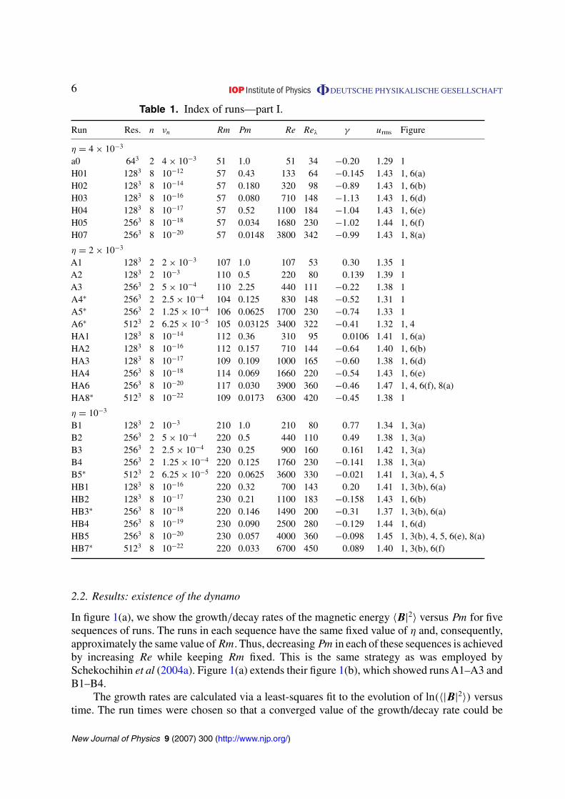
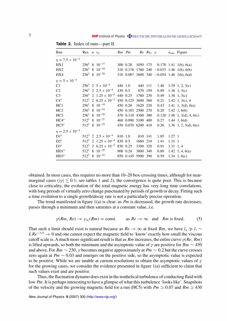
The maximum resolution that we could afford was 5123. All our runs are summarized intables 1 and 2, where we give for each run its resolution, the values of the (hyper)viscosityνn, Rm, Pm, Re, Reλ, the growth/decay rate γ , the rms velocity urms =

√〈|u|2〉, and a list of

figures in which this run appears. The runs marked with a star were done using a new codewritten by A Iskakov. All other runs were done using another code, written by J Maron, whichwas the code used in our earlier papers (Schekochihin et al 2004a, 2004b, 2005). Both codesare pseudospectral, solve the same equations (1) and (2) and use the same units of length andtime, but different time-stepping, fast Fourier transforms and parallelisation algorithms, as wellas slightly different implementations of the random forcing. We have checked conclusively thatA Iskakov’s code correctly reproduces the older results obtained with J Maron’s code.

New Journal of Physics 9 (2007) 300 (http://www.njp.org/)

6 DEUTSCHE PHYSIKALISCHE GESELLSCHAFT

Table 1. Index of runs—part I.

Run Res. n νn Rm Pm Re Reλ γ urms Figure

η = 4 × 10−3

a0 643 2 4 × 10−3 51 1.0 51 34 −0.20 1.29 1H01 1283 8 10−12 57 0.43 133 64 −0.145 1.43 1, 6(a)H02 1283 8 10−14 57 0.180 320 98 −0.89 1.43 1, 6(b)H03 1283 8 10−16 57 0.080 710 148 −1.13 1.43 1, 6(d)H04 1283 8 10−17 57 0.52 1100 184 −1.04 1.43 1, 6(e)H05 2563 8 10−18 57 0.034 1680 230 −1.02 1.44 1, 6(f)H07 2563 8 10−20 57 0.0148 3800 342 −0.99 1.43 1, 8(a)

η = 2 × 10−3

A1 1283 2 2 × 10−3 107 1.0 107 53 0.30 1.35 1A2 1283 2 10−3 110 0.5 220 80 0.139 1.39 1A3 2563 2 5 × 10−4 110 2.25 440 111 −0.22 1.38 1A4∗ 2563 2 2.5 × 10−4 104 0.125 830 148 −0.52 1.31 1A5∗ 2563 2 1.25 × 10−4 106 0.0625 1700 230 −0.74 1.33 1A6∗ 5123 2 6.25 × 10−5 105 0.03125 3400 322 −0.41 1.32 1, 4HA1 1283 8 10−14 112 0.36 310 95 0.0106 1.41 1, 6(a)HA2 1283 8 10−16 112 0.157 710 144 −0.64 1.40 1, 6(b)HA3 1283 8 10−17 109 0.109 1000 165 −0.60 1.38 1, 6(d)HA4 2563 8 10−18 114 0.069 1660 220 −0.54 1.43 1, 6(e)HA6 2563 8 10−20 117 0.030 3900 360 −0.46 1.47 1, 4, 6(f), 8(a)HA8∗ 5123 8 10−22 109 0.0173 6300 420 −0.45 1.38 1

η = 10−3

B1 1283 2 10−3 210 1.0 210 80 0.77 1.34 1, 3(a)B2 2563 2 5 × 10−4 220 0.5 440 110 0.49 1.38 1, 3(a)B3 2563 2 2.5 × 10−4 230 0.25 900 160 0.161 1.42 1, 3(a)B4 2563 2 1.25 × 10−4 220 0.125 1760 230 −0.141 1.38 1, 3(a)B5∗ 5123 2 6.25 × 10−5 220 0.0625 3600 330 −0.021 1.41 1, 3(a), 4, 5HB1 1283 8 10−16 220 0.32 700 143 0.20 1.41 1, 3(b), 6(a)HB2 1283 8 10−17 230 0.21 1100 183 −0.158 1.43 1, 6(b)HB3∗ 2563 8 10−18 220 0.146 1490 200 −0.31 1.37 1, 3(b), 6(a)HB4 2563 8 10−19 230 0.090 2500 280 −0.129 1.44 1, 6(d)HB5 2563 8 10−20 230 0.057 4000 360 −0.098 1.45 1, 3(b), 4, 5, 6(e), 8(a)HB7∗ 5123 8 10−22 220 0.033 6700 450 0.089 1.40 1, 3(b), 6(f)

2.2. Results: existence of the dynamo

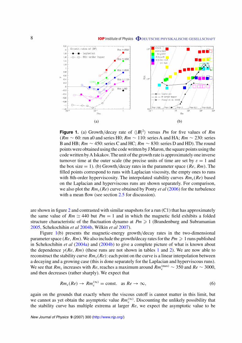
In figure 1(a), we show the growth/decay rates of the magnetic energy 〈B|2〉 versus Pm for fivesequences of runs. The runs in each sequence have the same fixed value of η and, consequently,approximately the same value of Rm. Thus, decreasing Pm in each of these sequences is achievedby increasing Re while keeping Rm fixed. This is the same strategy as was employed bySchekochihin et al (2004a). Figure 1(a) extends their figure 1(b), which showed runs A1–A3 andB1–B4.

The growth rates are calculated via a least-squares fit to the evolution of ln(〈|B|2〉) versustime. The run times were chosen so that a converged value of the growth/decay rate could be

New Journal of Physics 9 (2007) 300 (http://www.njp.org/)

7 DEUTSCHE PHYSIKALISCHE GESELLSCHAFT

Table 2. Index of runs—part II.

Run Res. n νn Rm Pm Re Reλ γ urms Figure

η = 7.5 × 10−4

HX1 2563 8 10−17 300 0.28 1050 175 0.178 1.41 1(b), 6(a)HX2 2563 8 10−18 310 0.176 1760 240 −0.033 1.46 1(b), 6(b)HX4 2563 8 10−20 310 0.087 3600 340 −0.054 1.46 1(b), 6(d)

η = 5 × 10−4

C1 2563 2 5 × 10−4 440 1.0 440 111 1.40 1.39 1, 2, 3(c)C2 2563 2 2.5 × 10−4 430 0.5 870 159 0.89 1.36 1, 3(c)C3 2563 2 1.25 × 10−4 440 0.25 1760 230 0.49 1.38 1, 3(c)C4∗ 5123 2 6.25 × 10−5 450 0.125 3600 360 0.21 1.42 1, 3(c), 4HC1 2563 8 10−18 450 0.28 1620 220 0.43 1.41 1, 3(d), 6(a)HC2 2563 8 10−19 450 0.183 2500 270 0.20 1.42 1, 6(b)HC3 2563 8 10−20 470 0.110 4300 380 0.120 1.48 1, 3(d), 4, 6(c)HC4∗ 5123 8 10−21 460 0.090 5100 400 0.27 1.44 1, 6(d)HC5∗ 5123 8 10−22 430 0.070 6200 410 0.26 1.36 1, 2, 3(d), 6(e)

η = 2.5 × 10−4

D1∗ 5123 2 2.5 × 10−4 810 1.0 810 141 1.85 1.27 1D2∗ 5123 2 1.25 × 10−4 830 0.5 1660 210 1.41 1.31 1D3∗ 5123 2 6.25 × 10−5 830 0.25 3300 320 0.91 1.31 1, 4HD1∗ 5123 8 10−20 900 0.24 3800 340 0.80 1.42 1, 4, 6(a)HD3∗ 5123 8 10−22 850 0.145 5900 390 0.59 1.34 1, 6(c)

obtained. In most cases, this requires no more than 10–20 box-crossing times, although for near-marginal cases (|γ| � 0.1; see tables 1 and 2), the convergence is quite poor. This is becauseclose to criticality, the evolution of the total magnetic energy has very long time correlations,with long periods of virtually zero change punctuated by periods of growth or decay. Fitting sucha time evolution to a single growth/decay rate is not a particularly precise operation.

The trend manifested in figure 1(a) is clear: as Pm is decreased, the growth rate decreases,passes through a minimum and then saturates at a constant value, i.e.

γ(Rm, Re) → γ∞(Rm) = const. as Re → ∞ and Rm is fixed. (5)

That such a limit should exist is natural because as Re → ∞ at fixed Rm, we have lη � lν ∼LRe−3/4 → 0 and one cannot expect the magnetic field to ‘know’ exactly how small the viscouscutoff scale is. A much more significant result is that as Rm increases, the entire curve γ(Re, Rm)

is lifted upwards, so both the minimum and the asymptotic value of γ are positive for Rm ∼ 450and above. For Rm ∼ 230, γ becomes negative approximately at Pm ∼ 0.2 but the curve crosseszero again at Pm ∼ 0.03 and emerges on the positive side, so the asymptotic value is expectedto be positive. While we are unable at current resolutions to obtain the asymptotic values of γ

for the growing cases, we consider the evidence presented in figure 1(a) sufficient to claim thatsuch values exist and are positive.

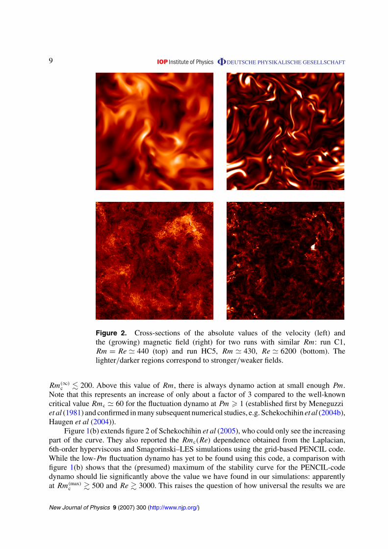
Thus, the fluctuation dynamo does exist in the nonhelical turbulence of conducting fluid withlow Pm. It is perhaps interesting to have a glimpse of what this turbulence ‘looks like’. Snapshotsof the velocity and the growing magnetic field for a run (HC5) with Pm 0.07 and Rm 430

New Journal of Physics 9 (2007) 300 (http://www.njp.org/)

8 DEUTSCHE PHYSIKALISCHE GESELLSCHAFT

(a) (b)

Figure 1. (a) Growth/decay rate of 〈|B|2〉 versus Pm for five values of Rm

(Rm ∼ 60: run a0 and series H0; Rm ∼ 110: series A and HA; Rm ∼ 230: seriesB and HB; Rm ∼ 450: series C and HC; Rm ∼ 830: series D and HD). The roundpoints were obtained using the code written by J Maron, the square points using thecode written byA Iskakov. The unit of the growth rate is approximately one inverseturnover time at the outer scale (the precise units of time are set by ε = 1 andthe box size = 1). (b) Growth/decay rates in the parameter space (Re, Rm). Thefilled points correspond to runs with Laplacian viscosity, the empty ones to runswith 8th-order hyperviscosity. The interpolated stability curves Rmc(Re) basedon the Laplacian and hyperviscous runs are shown separately. For comparison,we also plot the Rmc(Re) curve obtained by Ponty et al (2006) for the turbulencewith a mean flow (see section 2.5 for discussion).

are shown in figure 2 and contrasted with similar snapshots for a run (C1) that has approximatelythe same value of Rm 440 but Pm = 1 and in which the magnetic field exhibits a foldedstructure characteristic of the fluctuation dynamo at Pm � 1 (Brandenburg and Subramanian2005, Schekochihin et al 2004b, Wilkin et al 2007).

Figure 1(b) presents the magnetic-energy growth/decay rates in the two-dimensionalparameter space (Re, Rm). We also include the growth/decay rates for the Pm � 1 runs publishedin Schekochihin et al (2004a) and (2004b) to give a complete picture of what is known aboutthe dependence γ(Re, Rm) (these runs are not shown in tables 1 and 2). We are now able toreconstruct the stability curve Rmc(Re): each point on the curve is a linear interpolation betweena decaying and a growing case (this is done separately for the Laplacian and hyperviscous runs).We see that Rmc increases with Re, reaches a maximum around Rm(max)

c ∼ 350 and Re ∼ 3000,and then decreases (rather sharply). We expect that

Rmc(Re) → Rm(∞)c = const. as Re → ∞, (6)

again on the grounds that exactly where the viscous cutoff is cannot matter in this limit, butwe cannot as yet obtain the asymptotic value Rm(∞)

c . Discounting the unlikely possibility thatthe stability curve has multiple extrema at larger Re, we expect the asymptotic value to be

New Journal of Physics 9 (2007) 300 (http://www.njp.org/)

9 DEUTSCHE PHYSIKALISCHE GESELLSCHAFT

Figure 2. Cross-sections of the absolute values of the velocity (left) andthe (growing) magnetic field (right) for two runs with similar Rm: run C1,Rm = Re 440 (top) and run HC5, Rm 430, Re 6200 (bottom). Thelighter/darker regions correspond to stronger/weaker fields.

Rm(∞)c � 200. Above this value of Rm, there is always dynamo action at small enough Pm.

Note that this represents an increase of only about a factor of 3 compared to the well-knowncritical value Rmc 60 for the fluctuation dynamo at Pm � 1 (established first by Meneguzziet al (1981) and confirmed in many subsequent numerical studies, e.g. Schekochihin et al (2004b),Haugen et al (2004)).

Figure 1(b) extends figure 2 of Schekochihin et al (2005), who could only see the increasingpart of the curve. They also reported the Rmc(Re) dependence obtained from the Laplacian,6th-order hyperviscous and Smagorinski–LES simulations using the grid-based PENCIL code.While the low-Pm fluctuation dynamo has yet to be found using this code, a comparison withfigure 1(b) shows that the (presumed) maximum of the stability curve for the PENCIL-codedynamo should lie significantly above the value we have found in our simulations: apparentlyat Rm(max)

c � 500 and Re � 3000. This raises the question of how universal the results we are

New Journal of Physics 9 (2007) 300 (http://www.njp.org/)

10 DEUTSCHE PHYSIKALISCHE GESELLSCHAFT

reporting are. Another piece of numerical evidence that leads to the same question is the (smallbut measurable) difference between the stability curves reconstructed using the Laplacian andthe hyperviscous runs.

2.3. Laplacian versus hyperviscous simulations

As we argued in the introduction, it is reasonable to assume that whether or not the dynamoaction is present in the limit of Rm � Re → ∞ does not depend on the nature of the viscouscutoff. If this is true, demonstrating that it is present in the hyperviscous case should be sufficientto claim that it is present generally. It is also likely that the asymptotic value Rm(∞)

c will proveto be robust. However, the shape of the stability curve Rmc(Re) is certainly not universal.Indeed, let us consider what determines this shape in the transition region between Rmc 60 forPm � 1 and the yet undetermined asymptotic value Rm(∞)

c � 200 for Pm � 1. When Re � Rm

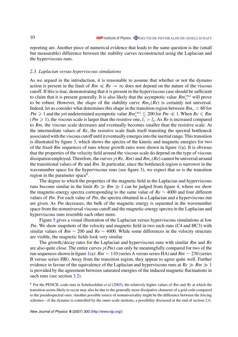
(Pm � 1), the viscous scale is larger than the resistive one, lν > lη. As Re is increased comparedto Rm, the viscous scale decreases and eventually becomes smaller than the resistive scale. Atthe intermediate values of Re, the resistive scale finds itself transiting the spectral bottleneckassociated with the viscous cutoff until it eventually emerges into the inertial range. This transitionis illustrated by figure 3, which shows the spectra of the kinetic and magnetic energies for twoof the fixed-Rm sequences of runs whose growth rates were shown in figure 1(a). It is obviousthat the properties of the velocity field around the viscous scale do depend on the type of viscousdissipation employed. Therefore, the curves γ(Re, Rm) and Rmc(Re) cannot be universal aroundthe transitional values of Re and Rm. In particular, since the bottleneck region is narrower in thewavenumber space for the hyperviscous runs (see figure 3), we expect that so is the transitionregion in the parameter space8.

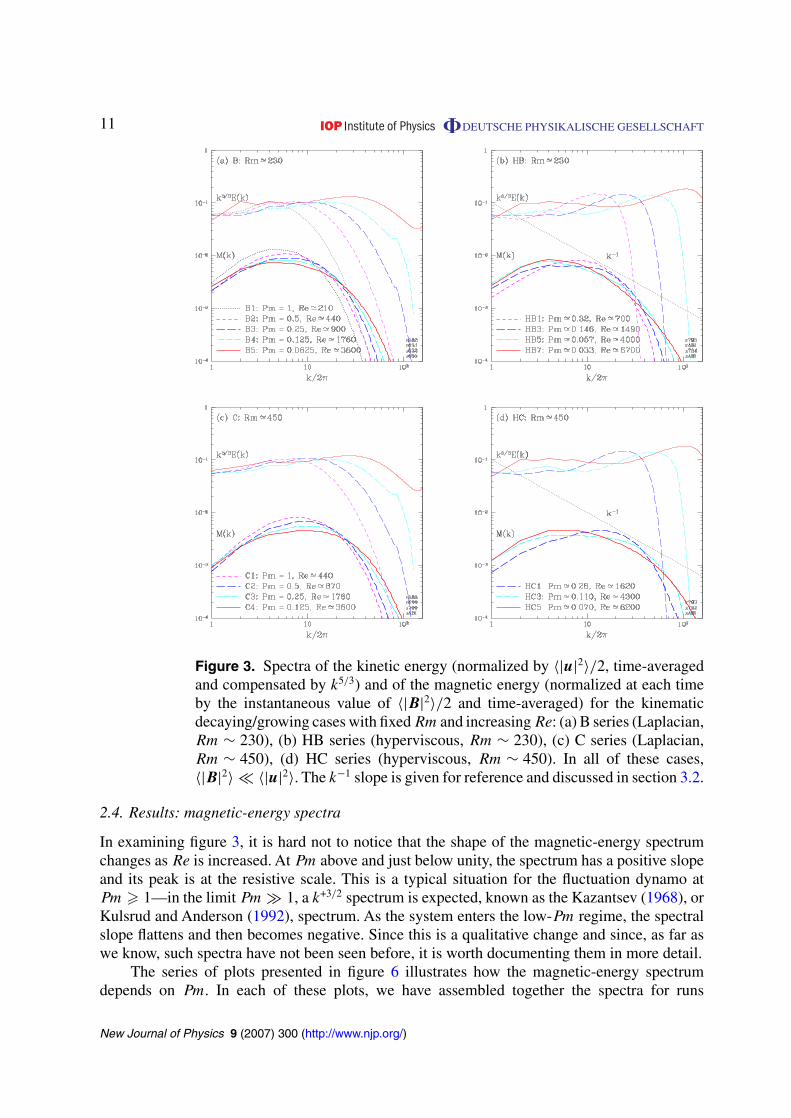
The degree to which the properties of the magnetic field in the Laplacian and hyperviscousruns become similar in the limit Re � Rm � 1 can be judged from figure 4, where we showthe magnetic-energy spectra corresponding to the same value of Re ∼ 4000 and four differentvalues of Pm. For each value of Pm, the spectra obtained in a Laplacian and a hyperviscous runare given. As Pm decreases, the bulk of the magnetic energy is separated in the wavenumberspace from the nonuniversal viscous cutoff and the magnetic-energy spectra in the Laplacian andhyperviscous runs resemble each other more.

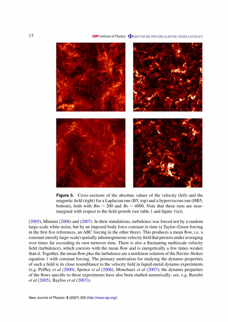
Figure 5 gives a visual illustration of the Laplacian versus hyperviscous simulations at lowPm. We show snapshots of the velocity and magnetic field in two such runs (C4 and HC3) withsimilar values of Rm ∼ 200 and Re ∼ 4000. While some differences in the velocity structureare visible, the magnetic fields look very similar.

The growth/decay rates for the Laplacian and hyperviscous runs with similar Rm and Re

are also quite close. The entire curves γ(Pm) can only be meaningfully compared for two of therun sequences shown in figure 1(a): Rm ∼ 110 (seriesA versus series HA) and Rm ∼ 230 (seriesB versus series HB). Away from the transition region, they appear to agree quite well. Furtherevidence in favour of the equivalence of the Laplacian and hyperviscous runs at Re � Rm � 1is provided by the agreement between saturated energies of the induced magnetic fluctuations insuch runs (see section 3.2).

8 For the PENCIL-code runs in Schekochihin et al (2005), the relatively higher values of Rm and Re at which thetransition seems likely to occur may also be due to the generally more dissipative character of a grid code comparedto the pseudospectral ones. Another possible source of nonuniversality might be the difference between the forcingschemes—if the dynamo is controlled by the outer-scale motions, a possibility discussed at the end of section 2.6.

New Journal of Physics 9 (2007) 300 (http://www.njp.org/)

11 DEUTSCHE PHYSIKALISCHE GESELLSCHAFT

Figure 3. Spectra of the kinetic energy (normalized by 〈|u|2〉/2, time-averagedand compensated by k5/3) and of the magnetic energy (normalized at each timeby the instantaneous value of 〈|B|2〉/2 and time-averaged) for the kinematicdecaying/growing cases with fixed Rm and increasing Re: (a) B series (Laplacian,Rm ∼ 230), (b) HB series (hyperviscous, Rm ∼ 230), (c) C series (Laplacian,Rm ∼ 450), (d) HC series (hyperviscous, Rm ∼ 450). In all of these cases,〈|B|2〉 � 〈|u|2〉. The k−1 slope is given for reference and discussed in section 3.2.

2.4. Results: magnetic-energy spectra

In examining figure 3, it is hard not to notice that the shape of the magnetic-energy spectrumchanges as Re is increased. At Pm above and just below unity, the spectrum has a positive slopeand its peak is at the resistive scale. This is a typical situation for the fluctuation dynamo atPm � 1—in the limit Pm � 1, a k+3/2 spectrum is expected, known as the Kazantsev (1968), orKulsrud and Anderson (1992), spectrum. As the system enters the low-Pm regime, the spectralslope flattens and then becomes negative. Since this is a qualitative change and since, as far aswe know, such spectra have not been seen before, it is worth documenting them in more detail.

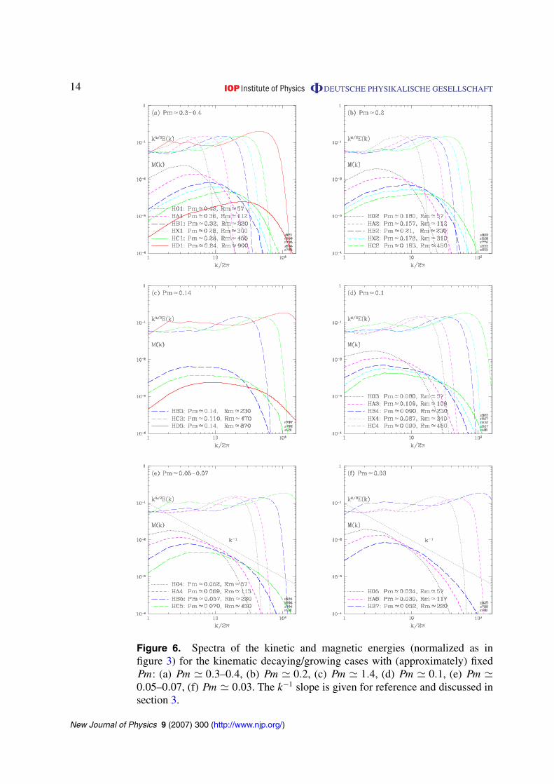
The series of plots presented in figure 6 illustrates how the magnetic-energy spectrumdepends on Pm. In each of these plots, we have assembled together the spectra for runs

New Journal of Physics 9 (2007) 300 (http://www.njp.org/)

12 DEUTSCHE PHYSIKALISCHE GESELLSCHAFT

Figure 4. Spectra of the kinetic and magnetic energies (normalized as in figure 3)for the kinematic decaying/growing cases with fixed Re 4000 and differentPm. For each value of Rm, we plot the spectra for a Laplacian (solid lines) anda hyperviscous (dashed lines) run. The kinetic-energy spectra are independentof Rm.

with different Rm and Re whose ratio was approximately equal to a chosen fixed value ofPm—approximately because for the hyperviscous case, one cannot fix Pm exactly beforeperforming the simulation (see (3) and (4)). Making allowances for this imprecision, it is stillpossible to conclude tentatively from figure 6 that the slope of the magnetic-energy spectrumdepends on Pm but not on individually on Re or Rm. As Pm decreases, the slope turnsfrom positive to negative. The data appears more consistent with the peak of the spectrumshifted towards the outer scale than with it moving with the resistive scale (lη ∼ LRm−3/4; seesection 2.6), but again, this is only a tentative conclusion.

Unfortunately, here as everywhere else, an attempt to establish numerically a solidasymptotic result is frustrated by the resolution constraints: in order to determine the spectralslope or the position of the spectral peak, we need to resolve the limit Re � Rm � 1 (i.e. bothPm � 1 and Rm � 1), but we cannot currently achieve sufficiently large values of Rm forPm � 1. We shall, therefore, not make any final statements here about the asymptotic form ofthe magnetic spectrum, although in figures 6(e) and (f) we did provide the reference slope of k−1

and will discuss it as a theoretical possibility in section 3.2.Note finally that the form of the spectrum does not change qualitatively between the growing

and decaying runs: for example, in figure 6(c), the magnetic energy in run HB3 decays while inruns HC3 and HD3 it grows, but the spectral slope appears to be the same.

2.5. Discussion: relation to results for turbulence with a mean flow

Since we have claimed above that the low-Pm fluctuation dynamo had not previously been seenin numerical simulations, it is important to explain how our results should be compared with theRmc(Re) dependences obtained in the recent numerical studies by Nore et al (1997), Ponty et al(2005), Mininni et al (2005), Ponty et al (2006), Laval et al (2006), Mininni and Montgomery

New Journal of Physics 9 (2007) 300 (http://www.njp.org/)

13 DEUTSCHE PHYSIKALISCHE GESELLSCHAFT

Figure 5. Cross-sections of the absolute values of the velocity (left) and themagnetic field (right) for a Laplacian run (B5, top) and a hyperviscous run (HB5,bottom), both with Rm ∼ 200 and Re ∼ 4000. Note that these runs are near-marginal with respect to the field growth (see table 1 and figure 1(a)).

(2005), Mininni (2006) and (2007). In their simulations, turbulence was forced not by a randomlarge-scale white noise, but by an imposed body force constant in time (a Taylor–Green forcingin the first five references, an ABC forcing in the other three). This produces a mean flow, i.e. aconstant (mostly large-scale) spatially inhomogeneous velocity field that persists under averagingover times far exceeding its own turnover time. There is also a fluctuating multiscale velocityfield (turbulence), which coexists with the mean flow and is energetically a few times weakerthan it. Together, the mean flow plus the turbulence are a nonlinear solution of the Navier–Stokesequation 1 with constant forcing. The primary motivation for studying the dynamo propertiesof such a field is its close resemblance to the velocity field in liquid-metal dynamo experiments(e.g. Peffley et al (2000), Spence et al (2006), Monchaux et al (2007); the dynamo propertiesof the flows specific to these experiments have also been studied numerically: see, e.g. Raveletet al (2005), Bayliss et al (2007)).

New Journal of Physics 9 (2007) 300 (http://www.njp.org/)

14 DEUTSCHE PHYSIKALISCHE GESELLSCHAFT

Figure 6. Spectra of the kinetic and magnetic energies (normalized as infigure 3) for the kinematic decaying/growing cases with (approximately) fixedPm: (a) Pm 0.3–0.4, (b) Pm 0.2, (c) Pm 1.4, (d) Pm 0.1, (e) Pm 0.05–0.07, (f) Pm 0.03. The k−1 slope is given for reference and discussed insection 3.

New Journal of Physics 9 (2007) 300 (http://www.njp.org/)

15 DEUTSCHE PHYSIKALISCHE GESELLSCHAFT

The mean flows that develop in such systems are usually dynamos by themselves—mean-field dynamos, to be precise (both in the case of helical mean flows like the ABC and inthe nonhelical case of the Taylor–Green forcing). They give rise to growing magnetic fieldsat scales larger than the scale of the flow (or comparable to it, when the scale of the meanflow is comparable to the size of the simulation box). For Pm � 1, the threshold for the fieldamplification is very low in these systems: Rmc ∼ 10, which is a typical situation for the mean-field dynamos (Brandenburg 2001, cf Galanti et al 1992). The presence of a large amount ofthe small-scale magnetic energy in these simulations should most probably be attributed to themagnetic induction, rather than to the fluctuation dynamo, because the growth is happening atvalues of Rm that are well below the fluctuation-dynamo threshold (Rmc ∼ 60 for Pm � 1; seefigure 1(b)).

As Pm is decreased, Rmc increases and eventually saturates at some larger value,giving rise to a stability curve Rmc(Re) that looks similar to the stability curve we haveobtained in our simulations. This similarity (enhanced sometimes by the ambiguity in thedefinitions of the Reynolds numbers) ought not to lead to any confusion between the twocurves. In order to illustrate the difference between them, we have plotted in figure 1(b)the stability curve reported by Ponty et al (2006) for their simulations with a Taylor–Greenforcing. The data are taken from their table 1 and calibrated according to our definitionsof Re and Rm: they define Re =

√〈|u|2〉 Ldyn/ν, where Ldyn is the dynamical integral scale

computed from the kinetic-energy spectrum and given in their table 1, while we define Re

according to (4). The box wavenumber k0 = 1 in their calculations. We see that the twocurves are very different: the dynamo threshold for the simulations with a mean flow is muchlower than for our homogeneous simulations. The difference is not merely quantitative: theordered large-scale structure of the growing magnetic field in the Pm ∼ 1 runs of Pontyet al (2005) (the lower part of their stability curve) confirms that it is a mean-field dynamo.

The increase of Rmc with increasing Re in these simulations has been attributed to theinterference by the turbulence with the dynamo properties of the mean flow—a manifestationof a tendency for higher dynamo thresholds in the presence a large-scale noise (Laval et al2006, Petrelis and Fauve 2006). It would be interesting to check whether the turbulence inthese simulations might itself act as a dynamo if the mean flow is ‘manually’ removed fromthe induction equation (2). Comparison of the two stability curves in figure 1(b) suggests thatin order for this to be the case, Rm must be increased very substantially—above the thresholdfound by us.

Let us conclude this discussion on a speculative note. while simulations with a mean flowundoubtedly exhibit a mean-field dynamo at Pm � 1, it is not clear whether that is also the casewhen Pm � 1. It may or may not be a coincidence that the low-Pm threshold for the simulationswith a mean flow appears to be very close to the large-Pm fluctuation-dynamo threshold. Sincethe mean flow most probably has chaotic Lagrangian trajectories (although this has not beenexplicitly checked), it should be a fluctuation dynamo—it belongs to the same class as the large-Pm dynamos because the flow is spatially smooth. Could the turbulence, while suppressingthe mean-field dynamo in the low-Pm regime, somehow fail to interfere with the fluctuationdynamo of the mean flow? There is not enough evidence or physical insight available to us tojudge the merits of this possibility—or of another, equally speculative one that we float at theend of section 2.6. Two aspects of the published numerical results that seem to support it arethe evidence of direct nonlocal transfer of energy from the outer scale (the mean flow) to thesmall-scale magnetic field (Mininni et al 2005) and the fact that the magnetic-energy spectra

New Journal of Physics 9 (2007) 300 (http://www.njp.org/)

16 DEUTSCHE PHYSIKALISCHE GESELLSCHAFT

reported by Ponty et al (2005) do not exhibit the tendency towards a negative slope discussedin section 2.4, but rather bear a strong resemblance to the typical k+3/2 spectra of the fluctuationdynamo at Pm � 1 see, e.g. Haugen et al 2004, Schekochihin et al 2004b).

2.6. Discussion: relation to theory and outstanding questions

Given the numerical certainty that the low-Pm fluctuation dynamo exists, there remain a numberof theoretical uncertainties about the nature of this dynamo. The key question is whether or notit is the inertial-range motions that amplify the magnetic energy.

Suppose Re � Rm � 1. Let us examine what can be achieved by assuming that the transferof the kinetic into magnetic energy is local in scale space9. For Kolmogorov turbulence, thecharacteristic velocity fluctuation at scale l is δul ∼ (εl)1/3, where ε is the total power injectedinto the turbulence (the turbulent energy flux). The characteristic rate of stretching of the magneticfield by the velocity field at scale l is then δul/ l ∼ ε1/3l−2/3. The characteristic rate of turbulentdiffusion at scale l is of the same order. Comparing the stretching rate with the rate of the Ohmicdiffusion of the magnetic field, η/l2, one finds the resistive scale, i.e. the scale at which thestretching rate is maximal and below which it is overcome by diffusion (Moffatt 1961):

lη ∼(

η3

ε

)1/4

∼ L

Rm3/4(7)

(this resistive scale does, indeed, lie inside the inertial range, L � lη � lν, where the viscousscale lν is estimated using (7) with η replaced by ν). Thus, if the local interaction of the inertial-range motions with the magnetic field is capable of amplifying the field in a sustained way, thegrowth rate of the magnetic energy should scale with Rm as

γ ∼ δulη

lη∼ ε1/3

l2/3η

∼(

ε

η

)1/2

∼ urms

LRm1/2 (8)

in the limit Re → ∞. This dynamo, if it exists, is purely a property of the inertial range and isindependent of any system-dependent outer-scale circumstances such as, e.g. the presence of amean flow. Given a large enough Rm, the growth rate (8) will always be larger than a mean-fieldor any other kind of dynamo associated with the outer-scale motions, because the latter cannotamplify the field faster than at the rate

γ ∼ U

L∼ urms

L, (9)

where U is the characteristic velocity at the outer scale.While our numerical results allowed us to make what we consider a compelling case for the

existence of a positive asymptotic value of the growth rate (section 2.2), we cannot at this stage

9 Whether it really is local should be the subject of a thorough future investigation, possibly along the lines of therecent study by Mininni et al (2005) of a mean-flow-driven dynamo. Note that the shell-model simulations recentlycarried out by Stepanov and Plunian (2007), which enforce the locality of interactions, return a picture that seemsto be broadly in agreement with the inertial-range dynamo scenario discussed below. On the other hand, EDQNMclosure simulations do not find any increase in Rmc for Pm � 1 compared with Pm � 1 (Leorat et al 1981).

New Journal of Physics 9 (2007) 300 (http://www.njp.org/)

17 DEUTSCHE PHYSIKALISCHE GESELLSCHAFT

check whether it scales with Rm according to (8) or reaches an Rm-independent limit as in (9).Neither of these possibilities can be ruled out a priori.

Should the scaling (8) be confirmed, the case for an inertial-range dynamo would becomplete. This case is strengthened somewhat by the theoretical predictions based on the onlyavailable model of the turbulent dynamo that is solvable exactly—the Kazantsev (1968) model.This model considers a Gaussian random velocity field that is a white noise in time. The salientproperty of the inertial-range velocities is their spatial roughness: δul ∼ l1/3 for L � l � lνcompared with a smooth velocity δul ∼ l for l � lν. This is mimicked by prescribing a spatiallyrough power-law correlation function for the Kazantsev model field. For a certain range ofexponents of this power law, it is then possible to show analytically that the Kazantsev fieldis a dynamo (Arponen and Horvai 2006, Boldyrev and Cattaneo 2004, Celani et al 2006,Rogachevskii and Kleeorin 1997,Vincenzi 2002). The difficulty lies in establishing a quantitativeconnection between this result and the real turbulence, in which the decorrelation time of theinertial-range motions is certainly not small but comparable to their turnover time and scale-dependent ∼ l2/3. It is not known whether setting it to zero changes the dynamo properties of thevelocity field enough to render the white-noise model irrelevant. If the white-noise velocity is onsome level acceptable, it is not known what choice of its roughness exponent (which determineswhether it is a dynamo!) makes it a good model of the inertial-range turbulent velocity field. Theauthors cited above used a plausible argument (first suggested by Vainshtein 1982), which ledthem to predict dynamo action. However, this prediction is purely a quantitative mathematicaloutcome of analysing a synthetic velocity field that is at best a passable qualitative representationof real turbulence. In the absence of a physical model of the inertial-range dynamo, the validityof this prediction remains in doubt.

It is natural to ask whether any of the quantitative predictions based on the Kazantsev modelare borne out by our numerical results. One such prediction is the scaling (8) of the growth rate,which cannot as yet be verified numerically. Another, due to Rogachevskii and Kleeorin (1997)and to Boldyrev and Cattaneo (2004), is the expectation that the asymptotic dynamo thresholdRm(∞)

c for Pm � 1 should be approximately 7 times higher than a similar threshold Rmc ∼ 60for the Pm � 1 case (see figure 1(b); in the Kazantsev model, the latter threshold is computed byusing a velocity field with a smooth spatial correlator, see Novikov et al (1983)). This would implyRm(∞)

c ∼ 400, which is an overestimate by at least a factor of 2 (see section 2.2)—certainly nota damning contradiction, but somewhat short of a confirmation of the theory. Finally, Boldyrevand Cattaneo (2004) predict a (stretched) exponential fall off of the magnetic-field correlationfunction at l > lη, so the magnetic energy is concentrated sharply at the resistive scale. Thisappears to be at odds with the trend for the magnetic-energy spectrum to develop a negativeslope above the resistive scale, reported in section 2.4 (for example, a k−1 spectrum would implythat δBl ∼ constant, i.e. the correlation function is flat rather than falling off exponentially). Wereiterate, however, that at resolutions currently available to us, we are unable to claim definitivelythat the spectral peak is not, in fact, at the resistive scale.

Is there an alternative to the inertial-range dynamo? It might be worth asking whetherthe randomly forced outer-scale motions could act as a dynamo despite (or in concert with)the turbulence in the inertial range. Indeed, how essential is the physical difference betweenthe outer-scale motion, whose decorrelation time (∼L/U) is long compared with the inertial-range motions, and a mean flow, whose correlation time in infinite? Can both the mean-flow-driven dynamo found by Ponty et al (2005) and the fluctuation dynamo reported here by us bemanifestations of some universal basic mechanism—for example, of the field amplification by

New Journal of Physics 9 (2007) 300 (http://www.njp.org/)

18 DEUTSCHE PHYSIKALISCHE GESELLSCHAFT

a combined action of a persistent (slowly changing) large-scale (outer-scale) shear and small-scale (inertial-range) turbulent fluctuations (a nonhelical mean-field dynamo of this type hasbeen proposed theoretically by Rogachevskii and Kleeorin (2003))?

An unambiguous signature of this or any other type of outer-scale-driven dynamo wouldbe the convergence of the growth rate to an Rm-independent limit (9). One way to investigatenumerically whether there is a smooth connection between the mean-flow dynamo and therandomly forced one would be to construct stability curves Rmc(Re) for a series of numericalexperiments with an inhomogeneous body force (similar to Ponty et al 2005), which however, isartificially decorrelated with a prescribed correlation time τcorr. The limit τcorr = ∞ correspondsto the turbulence with a mean flow. As τcorr is reduced, the mean flow should develop a slow timedependence and at τcorr ∼ L/U, the situation would become equivalent to the randomly forcedcase discussed here.

3. Turbulent induction

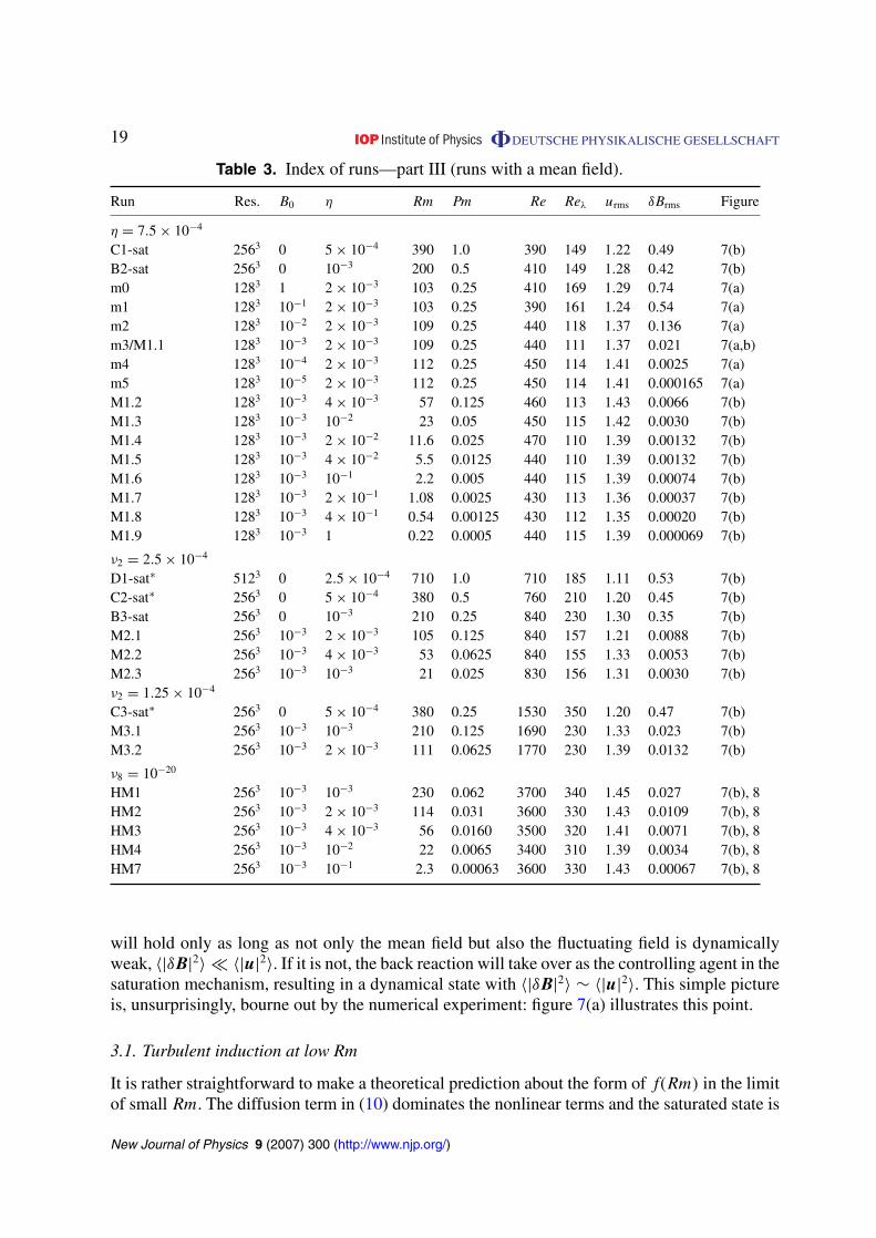
The turbulent magnetic induction is the tangling of a uniform (or large-scale) mean magneticfield by turbulence, which produces magnetic energy at small scales. The mean field may bedue to some external imposition or to a mean-field dynamo. Broadly speaking, whatever is themechanism that generates and/or maintains a magnetic field, the turbulent induction is a nonlocalenergy transfer process whereby this field couples to motions at smaller scales to give rise tomagnetic fluctuations at those scales. In any real system, it is only a part of a bigger picture of howthe magnetic field is generated and shaped. Given a multiscale observed or simulated magneticfield, one does not generally have enough information (or understanding), to tell whether it hasoriginated from the fluctuation dynamo, from the mean-field dynamo plus the turbulent inductionor from some combination of the two. However, in the computer, the turbulent-induction effectcan be isolated by measuring the response to an imposed uniform field in the subcritical cases,in which the magnetic field would otherwise decay (this approach has been popular in liquid-metal experiments; see, e.g. Bourgoin et al (2002), Odier et al (1998), Spence et al (2006)).Table 3 details a number of such runs, done using the same numerical set-up as that detailed insection 2.1. We shall see that examining their properties is both instructive in itself and may berevealing about the nature of the fluctuation dynamo.

Mathematically, if the magnetic field is represented as a sum of a uniform mean field and afluctuating part, B = B0 + δB, the fluctuating field satisfies

∂δB

∂t+ u · ∇δB = δB · ∇u + η∇2δB + B0 · ∇u. (10)

This is simply the induction equation (2) with a source term, which, in the absence of dynamoaction, will give rise to a saturated level of the magnetic-fluctuation energy. Equation (10) islinear in δB. Therefore, for dynamically weak mean fields, the saturated magnetic energy shouldbe proportional to the mean-field energy:

〈|δB|2〉 = f(Rm)B20. (11)

The coefficient of proportionality f(Rm) in this relation is expected to be an increasing functionof Rm. At large Rm, this coefficient can be large, f(Rm) � 1 and the relation equation (11)

New Journal of Physics 9 (2007) 300 (http://www.njp.org/)

19 DEUTSCHE PHYSIKALISCHE GESELLSCHAFT

Table 3. Index of runs—part III (runs with a mean field).

Run Res. B0 η Rm Pm Re Reλ urms δBrms Figure

η = 7.5 × 10−4

C1-sat 2563 0 5 × 10−4 390 1.0 390 149 1.22 0.49 7(b)B2-sat 2563 0 10−3 200 0.5 410 149 1.28 0.42 7(b)m0 1283 1 2 × 10−3 103 0.25 410 169 1.29 0.74 7(a)m1 1283 10−1 2 × 10−3 103 0.25 390 161 1.24 0.54 7(a)m2 1283 10−2 2 × 10−3 109 0.25 440 118 1.37 0.136 7(a)m3/M1.1 1283 10−3 2 × 10−3 109 0.25 440 111 1.37 0.021 7(a,b)m4 1283 10−4 2 × 10−3 112 0.25 450 114 1.41 0.0025 7(a)m5 1283 10−5 2 × 10−3 112 0.25 450 114 1.41 0.000165 7(a)M1.2 1283 10−3 4 × 10−3 57 0.125 460 113 1.43 0.0066 7(b)M1.3 1283 10−3 10−2 23 0.05 450 115 1.42 0.0030 7(b)M1.4 1283 10−3 2 × 10−2 11.6 0.025 470 110 1.39 0.00132 7(b)M1.5 1283 10−3 4 × 10−2 5.5 0.0125 440 110 1.39 0.00132 7(b)M1.6 1283 10−3 10−1 2.2 0.005 440 115 1.39 0.00074 7(b)M1.7 1283 10−3 2 × 10−1 1.08 0.0025 430 113 1.36 0.00037 7(b)M1.8 1283 10−3 4 × 10−1 0.54 0.00125 430 112 1.35 0.00020 7(b)M1.9 1283 10−3 1 0.22 0.0005 440 115 1.39 0.000069 7(b)

ν2 = 2.5 × 10−4

D1-sat∗ 5123 0 2.5 × 10−4 710 1.0 710 185 1.11 0.53 7(b)C2-sat∗ 2563 0 5 × 10−4 380 0.5 760 210 1.20 0.45 7(b)B3-sat 2563 0 10−3 210 0.25 840 230 1.30 0.35 7(b)M2.1 2563 10−3 2 × 10−3 105 0.125 840 157 1.21 0.0088 7(b)M2.2 2563 10−3 4 × 10−3 53 0.0625 840 155 1.33 0.0053 7(b)M2.3 2563 10−3 10−3 21 0.025 830 156 1.31 0.0030 7(b)ν2 = 1.25 × 10−4

C3-sat∗ 2563 0 5 × 10−4 380 0.25 1530 350 1.20 0.47 7(b)M3.1 2563 10−3 10−3 210 0.125 1690 230 1.33 0.023 7(b)M3.2 2563 10−3 2 × 10−3 111 0.0625 1770 230 1.39 0.0132 7(b)

ν8 = 10−20

HM1 2563 10−3 10−3 230 0.062 3700 340 1.45 0.027 7(b), 8HM2 2563 10−3 2 × 10−3 114 0.031 3600 330 1.43 0.0109 7(b), 8HM3 2563 10−3 4 × 10−3 56 0.0160 3500 320 1.41 0.0071 7(b), 8HM4 2563 10−3 10−2 22 0.0065 3400 310 1.39 0.0034 7(b), 8HM7 2563 10−3 10−1 2.3 0.00063 3600 330 1.43 0.00067 7(b), 8

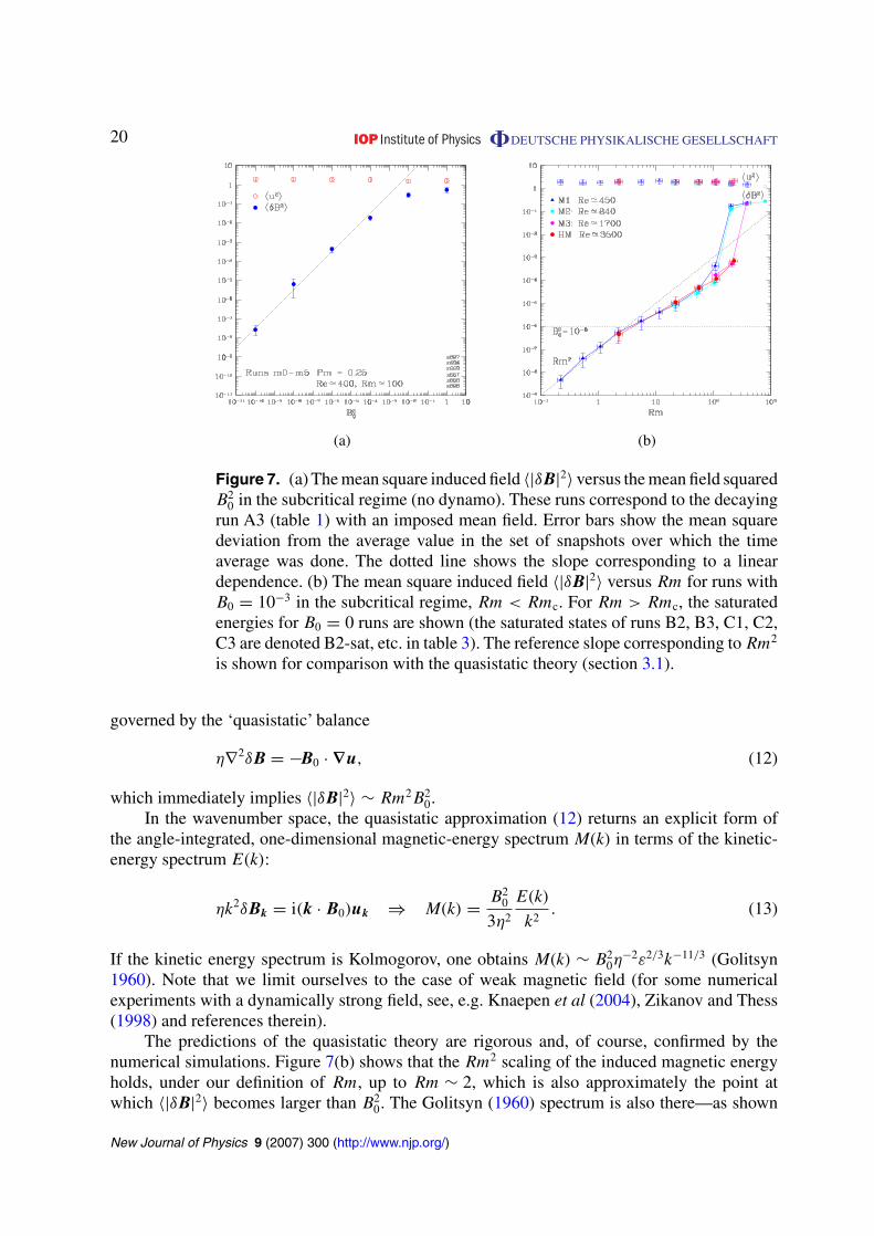
will hold only as long as not only the mean field but also the fluctuating field is dynamicallyweak, 〈|δB|2〉 � 〈|u|2〉. If it is not, the back reaction will take over as the controlling agent in thesaturation mechanism, resulting in a dynamical state with 〈|δB|2〉 ∼ 〈|u|2〉. This simple pictureis, unsurprisingly, bourne out by the numerical experiment: figure 7(a) illustrates this point.

3.1. Turbulent induction at low Rm

It is rather straightforward to make a theoretical prediction about the form of f(Rm) in the limitof small Rm. The diffusion term in (10) dominates the nonlinear terms and the saturated state is

New Journal of Physics 9 (2007) 300 (http://www.njp.org/)

20 DEUTSCHE PHYSIKALISCHE GESELLSCHAFT

(a) (b)

Figure 7. (a) The mean square induced field 〈|δB|2〉 versus the mean field squaredB2

0 in the subcritical regime (no dynamo). These runs correspond to the decayingrun A3 (table 1) with an imposed mean field. Error bars show the mean squaredeviation from the average value in the set of snapshots over which the timeaverage was done. The dotted line shows the slope corresponding to a lineardependence. (b) The mean square induced field 〈|δB|2〉 versus Rm for runs withB0 = 10−3 in the subcritical regime, Rm < Rmc. For Rm > Rmc, the saturatedenergies for B0 = 0 runs are shown (the saturated states of runs B2, B3, C1, C2,C3 are denoted B2-sat, etc. in table 3). The reference slope corresponding to Rm2

is shown for comparison with the quasistatic theory (section 3.1).

governed by the ‘quasistatic’ balance

η∇2δB = −B0 · ∇u, (12)

which immediately implies 〈|δB|2〉 ∼ Rm2B20.

In the wavenumber space, the quasistatic approximation (12) returns an explicit form ofthe angle-integrated, one-dimensional magnetic-energy spectrum M(k) in terms of the kinetic-energy spectrum E(k):

ηk2δBk = i(k · B0)uk ⇒ M(k) = B20

3η2

E(k)

k2. (13)

If the kinetic energy spectrum is Kolmogorov, one obtains M(k) ∼ B20η

−2ε2/3k−11/3 (Golitsyn1960). Note that we limit ourselves to the case of weak magnetic field (for some numericalexperiments with a dynamically strong field, see, e.g. Knaepen et al (2004), Zikanov and Thess(1998) and references therein).

The predictions of the quasistatic theory are rigorous and, of course, confirmed by thenumerical simulations. Figure 7(b) shows that the Rm2 scaling of the induced magnetic energyholds, under our definition of Rm, up to Rm ∼ 2, which is also approximately the point atwhich 〈|δB|2〉 becomes larger than B2

0. The Golitsyn (1960) spectrum is also there—as shown

New Journal of Physics 9 (2007) 300 (http://www.njp.org/)

21 DEUTSCHE PHYSIKALISCHE GESELLSCHAFT

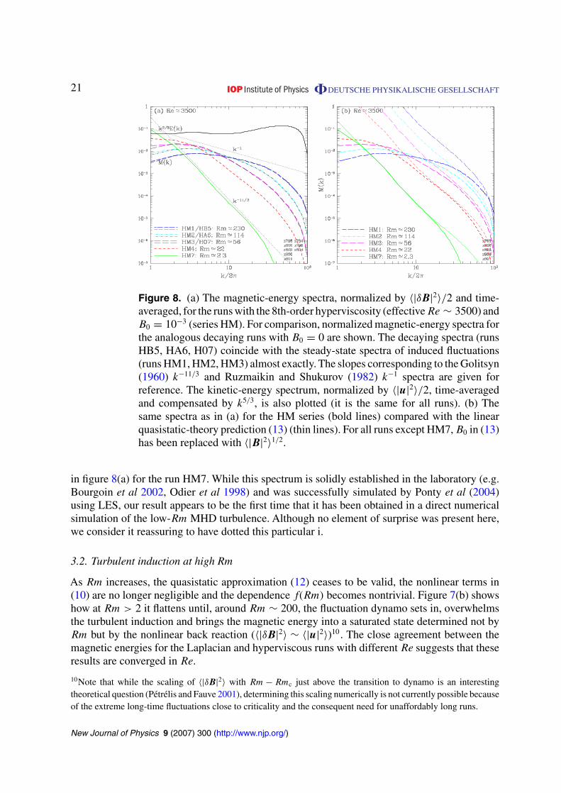
Figure 8. (a) The magnetic-energy spectra, normalized by 〈|δB|2〉/2 and time-averaged, for the runs with the 8th-order hyperviscosity (effective Re ∼ 3500) andB0 = 10−3 (series HM). For comparison, normalized magnetic-energy spectra forthe analogous decaying runs with B0 = 0 are shown. The decaying spectra (runsHB5, HA6, H07) coincide with the steady-state spectra of induced fluctuations(runs HM1, HM2, HM3) almost exactly. The slopes corresponding to the Golitsyn(1960) k−11/3 and Ruzmaikin and Shukurov (1982) k−1 spectra are given forreference. The kinetic-energy spectrum, normalized by 〈|u|2〉/2, time-averagedand compensated by k5/3, is also plotted (it is the same for all runs). (b) Thesame spectra as in (a) for the HM series (bold lines) compared with the linearquasistatic-theory prediction (13) (thin lines). For all runs except HM7, B0 in (13)has been replaced with 〈|B|2〉1/2.

in figure 8(a) for the run HM7. While this spectrum is solidly established in the laboratory (e.g.Bourgoin et al 2002, Odier et al 1998) and was successfully simulated by Ponty et al (2004)using LES, our result appears to be the first time that it has been obtained in a direct numericalsimulation of the low-Rm MHD turbulence. Although no element of surprise was present here,we consider it reassuring to have dotted this particular i.

3.2. Turbulent induction at high Rm

As Rm increases, the quasistatic approximation (12) ceases to be valid, the nonlinear terms in(10) are no longer negligible and the dependence f(Rm) becomes nontrivial. Figure 7(b) showshow at Rm > 2 it flattens until, around Rm ∼ 200, the fluctuation dynamo sets in, overwhelmsthe turbulent induction and brings the magnetic energy into a saturated state determined not byRm but by the nonlinear back reaction (〈|δB|2〉 ∼ 〈|u|2〉)10. The close agreement between themagnetic energies for the Laplacian and hyperviscous runs with different Re suggests that theseresults are converged in Re.

10Note that while the scaling of 〈|δB|2〉 with Rm − Rmc just above the transition to dynamo is an interestingtheoretical question (Petrelis and Fauve 2001), determining this scaling numerically is not currently possible becauseof the extreme long-time fluctuations close to criticality and the consequent need for unaffordably long runs.

New Journal of Physics 9 (2007) 300 (http://www.njp.org/)

22 DEUTSCHE PHYSIKALISCHE GESELLSCHAFT

While one might dwell on the question of what the asymptotic form of f(Rm) for largeRm should be (e.g. Cattaneo et al 1995, Low 1972, Moffatt 1961, Parker 1969, Saffman 1964,Vainshtein and Cattaneo 1992), it is perhaps reasonable to ask first whether, in view of our claimthat the fluctuation dynamo is unavoidable at sufficiently large Rm, the problem is meaningfullyposed. The short answer is, obviously, no. However, there is a useful way, already intimated atthe beginning of section 3, in which the turbulent induction problem can be posed at high Rm.

Firstly, if B0 is interpreted as the dynamo-generated field at the resistive scale and above,we may inquire into the behaviour of the magnetic fluctuations below the resistive scale, l � lη.Since the inertial-range motions at these scales have a shorter correlation time than at l ∼ lη, wecan, indeed, treat this as a problem with a constant mean field and use (10). The quasistatic theoryis still valid because the diffusion term is dominant. Thus, the Golitsyn (1960) spectrum is nowrecovered as the subresistive tail of the magnetic-energy spectrum (Moffatt 1961). In numericalsimulations, this is hard to check at current resolutions, but we can compare the magnetic spectrain our simulations with the quasistatic prediction (13) using the full numerically obtained formof E(k) and replacing B0 → 〈|B|2〉1/2. There is, indeed, a fit below some sufficiently small(resistive) scale, which predictably decreases with increasing Rm.

Secondly, if the dynamo amplifies the magnetic field at the outer scale or above (this isnow our mean field B0), one might ask how much magnetic energy this will generate via theturbulent induction in the part of the inertial range that lies above the resistive scale, L � l � lη.In (10), the diffusive term can now be ignored. It seems then to be a plausible argument that,if the nonlocal energy transfer from the outer-scale field is important at all, its effect on theinertial-range magnetic fluctuations can be found by balancing the ‘source’ term containing B0

with the nonlinear terms, which represent the local interactions between u and δB. This gives(Ruzmaikin and Shukurov 1982)

δBl ∼ B0 ⇒ M(k) ∼ B20k

−1. (14)

The same spectrum and the consequent scaling 〈|δB|2〉 ∼ (ln Rm)B20 were obtained in several

closure calculations assuming a weak mean field and no dynamo (Kleeorin and Rogachevskii1994, Kleeorin et al 1990, 1996) (see, however, an argument by Moffatt (1961), based on themathematical analogy between the magnetic field and vorticity and leading to a k1/3 spectrum).Note that all this only applies in the limit 〈|δB|2〉 � 〈|u|2〉 (which is where our simulations are;see figure 7(b)). Otherwise, dynamical effects, such as the Alfvenization of the turbulence, willbe important and determine the shape of the saturated state.

The scaling (14) can only be realized if an outer-scale magnetic field really exists and if thetangling of this field by turbulence is not superseded by an inertial-range dynamo, as discussedin section 2.6. Thus, it is only a possibility and, indeed, a signature property, if the fluctuationdynamo found by us is, in fact, an outer-scale dynamo. As we explained in section 2.4, ournumerical simulations are not sufficiently asymptotic to determine the spectrum of magneticfluctuations. The apparent tendency towards a negative spectral slope reported in section 2.4may be a telling sign in view of the theoretical result (14). We have plotted the reference k−1

slopes in figures 3, 6(e) and (f). We leave it to the reader’s judgement to decide if this scalingmight, indeed, be emerging there.

An important observation must be made in this context. The saturated magnetic-energyspectra in the subcritical runs with an imposed weak mean field turn out, after normalization,to be exactly the same as the normalized spectra of the corresponding decaying runs without

New Journal of Physics 9 (2007) 300 (http://www.njp.org/)

23 DEUTSCHE PHYSIKALISCHE GESELLSCHAFT

the mean field (see figure 8(a)). Furthermore, as reported in section 2.4, no qualitative changeoccurs in the magnetic-energy spectrum as the dynamo threshold is crossed. This seems to tellus that the same mechanism is responsible for setting the shape of the spectrum of the magneticfluctuations induced by a mean field and of the decaying or growing such fluctuations in theabsence of a mean field.

4. Conclusions

Let us reiterate the main numerical results and theoretical points presented above.

1. A fluctuation dynamo exists in the nonhelical randomly forced homogeneous turbulence ofa conducting fluid with low magnetic Prandtl number (section 2.2). The critical magneticReynolds number for this dynamo is at most three times larger than for Pm � 1: definedby (4), it is Rmc � 200 for Re � 6000, although there is a larger peak value at a somewhatsmaller Re.

2. The nature of the dynamo and its stability curve Rmc(Re) are different from the dynamoobtained in simulations and liquid-metal experiments with a mean flow (section 2.5).

3. The physical mechanism that enables the sustained growth of magnetic fluctuations in thelow-Pm regime is unknown. It is not as yet possible to determine numerically whetherthe fluctuation dynamo is driven by the inertial-range motions at the resistive scale andconsequently has a growth rate ∝ Rm1/2 in the limit Rm → ∞, or rather a constant growthrate comparable to the turnover rate of the outer-scale motions (section 2.6).

4. The magnetic-energy spectra in the low-Pm regime are qualitatively different from thePm � 1 case and appear to develop a negative spectral slope, which may be consistent withk−1, but cannot be definitively resolved (section 2.4). The spectra of the growing field aresimilar to those for the decaying field at lower Rm and to the saturated spectra of the inducedmagnetic energy in the presence of a weak mean field (section 3.2).

5. At very low Rm, the magnetic fluctuations induced via the tangling by turbulence of aweak mean field are well described by the quasistatic approximation. The k−11/3 spectrumis confirmed (section 3.1).

While these results leave a frustrating number of questions unanswered and do not entirelyclear up the confusion over the exact nature of the low-Pm dynamo, they do at least confirm thatthe object of this confusion exists. It is important to check in independent numerical experimentsboth that our conclusions hold and whether the value of the dynamo threshold obtained by us isuniversal. Some promising numerical experiments aimed at elucidating the nature of the dynamoand the role of the mean flow are proposed in sections 2.5 and 2.6.

The main conclusion of this work is the confirmation that nature will always find a wayto make a magnetic field where turbulence of a conducting fluid is present. In the astrophysicalcontext, the low-Pm fluctuation dynamo is particularly (although by no means solely) importantin the context of solar magnetism. While there is ample observational evidence that small-scalemagnetic fluctuations pervade the solar photosphere (e.g. Domınguez Cerdeña et al 2003, Socas-Navarro and Lites 2004, Solanki et al 2006, Trujillo Bueno et al 2004), the numerical evidenceused to argue that the turbulent fluctuation dynamo is responsible has thus far been basedon numerical simulations with Pm � 1 (Bushby 2007, Cattaneo 1999, Cattaneo et al 2003).The existence of the low-Pm fluctuation dynamo that we have established for an idealized

New Journal of Physics 9 (2007) 300 (http://www.njp.org/)

24 DEUTSCHE PHYSIKALISCHE GESELLSCHAFT

homogeneous MHD turbulence gives us confidence that attempts to demonstrate self-consistentmagnetic-field amplification in more realistic simulations of solar convection with Pm � 1 willeventually prove successful.

Acknowledgments

We thank A Brandenburg, B Dubrulle, S Fauve, C Forest, N Haugen, D Hughes, N Kleeorin, PMininni, J Papaloizou, J-F Pinton, F Plunian, Y Ponty, F Rincon, I Rogachevskii, A Shukurovand N Weiss for valuable discussions at various stages of this project. We are grateful to VDecyk (UCLA) who has kindly provided his FFT libraries from the UPIC framework. A A S wassupported by a PPARC Advanced Fellowship. He also thanks the USDOE Center for MultiscalePlasma Dynamic for travel support and the UCLA Plasma Group for its hospitality. A B I wassupported by the USDOE Center for Multiscale Plasma Dynamics. T A Y was supported bya UKAFF Fellowship and the Newton Trust. Simulations were done on UKAFF (Leicester),NCSA (Illinois) and the Dawson cluster (UCLA Plasma Group).

References

Arponen H and Horvai P 2006 Preprint nlin.CD/0610023Batchelor G K 1950 Proc. R. Soc. Lond. A 201 405Bayliss R A, Forest C B, Nornberg M D, Spence E J and Terry P W 2007 Phys. Rev. E 75 026303Berhanu M et al 2007 Europhys. Lett. 77 59001Boldyrev S and Cattaneo F 2004 Phys. Rev. Lett. 92 144501Bourgoin M et al 2002 Phys. Fluids 14 3046Brandenburg A 2001 Astrophys. J. 550 824Brandenburg A, Jennings R L, Nordlund Å, Rieutord M, Stein R F and Tuominen I 1996 J. Fluid Mech. 306 325Brandenburg A and Subramanian K 2005 Phys. Rep. 417 1Bushby P 2007 private communicationCattaneo F 1999 Astrophys. J. 515 L39Cattaneo F, Emonet T and Weiss N 2003 Astrophys. J. 588 1183Cattaneo F, Kim E J, Proctor M and Tao L 1995 Phys. Rev. Lett. 75 1522Celani A, Mazzino A and Vincenzi D 2006 Proc. R. Soc. Lond. A 462 137Chertkov M, Falkovich G, Kolokolov I and Vergassola M 1999 Phys. Rev. Lett. 83 4065Childress S and Gilbert A 1995 Stretch, Twist, Fold: The Fast Dynamo ( Berlin: Springer)Christensen U, Olson P and Glatzmaier G A 1999 Geophys. J. Int. 138 393Domınguez Cerdeña I, Sánchez Almeida J and Kneer F 2003 Astron. Astrophys. 407 741Galanti B, Sulem P L and Pouquet A 1992 Geophys. Astrophys. Fluid Dyn. 66 183Galloway D J and Proctor M R E 1992 Nature 356 691Golitsyn G S 1960 Sov. Phys.—Dokl. 5 536Haugen N E L, Brandenburg A and Dobler W 2004 Phys. Rev. E 70 016308Iskakov A B, Schekochihin A A, Cowley S C, McWilliams J C and Proctor M R E 2007 Preprint astro-ph/0702291Kazantsev A P 1968 Sov. Phys.—JETP 26 1031Kleeorin N, Mond M and Rogachevskii I 1996 Astron. Astrophys. 307 293Kleeorin N and Rogachevskii I 1994 Phys. Rev. E 50 2716Kleeorin N, Rogachevskii I and Ruzmaikin A 1990 Sov. Phys.—JETP 70 878Knaepen B, Kassinos S and Carati D 2004 J. Fluid Mech. 513 199Kulsrud R M and Anderson S W 1992 Astrophys. J. 396 606Laval J P, Blaineau P, Leprovost N, Dubrulle B and Daviaud F 2006 Phys. Rev. Lett. 96 204503

New Journal of Physics 9 (2007) 300 (http://www.njp.org/)

25 DEUTSCHE PHYSIKALISCHE GESELLSCHAFT

Leorat J, Pouquet A and Frisch U 1981 J. Fluid Mech. 104 419Low B C 1972 Astrophys. J. 173 549Meneguzzi M, Frisch U and Pouquet A 1981 Phys. Rev. Lett. 47 1060Mininni P, Alexakis A and Pouquet A 2005 Phys. Rev. E 72 046302Mininni P D 2006 Phys. Plasmas 13 056502Mininni P D 2007 Preprint physics/0702109Mininni P D and Montgomery D C 2005 Phys. Rev. E 72 056320Mininni P, Ponty Y, Montgomery D C, Pinton J F, Politano H and Pouquet A 2005 Astrophys. J. 626 853Moffatt H K 1978 Magnetic Field Generation in Electrically Conducting Fluids (Cambridge: Cambridge University

Press)Moffatt H K and Saffman P G 1963 Phys. Fluids 7 155Moffatt K 1961 J. Fluid Mech. 11 625Monchaux R et al 2007 Phys. Rev. Lett. 98 044502Nordlund Å, Brandenburg A, Jennings R L, Rieutord M, Ruokolainen J, Stein R F and Tuominen I 1992 Astrophys.

J. 392 647Nore C, Brachet M E, Politano H and Pouquet A 1997 Phys. Plasmas 4 1Novikov V G, Ruzmaikin A A and Sokoloff D D 1983 Sov. Phys.—JETP 58 527Odier P, Pinton J F and Fauve S 1998 Phys. Rev. E 58 7397Ossendrijver M 2003 Astron. Astrophys. Rev. 11 287Ott E 1998 Phys. Plasmas 5 1636Parker E N 1969 Astrophys. J. 138 226Peffley N L, Cawthorne A B and Lathrop D P 2000 Phys. Rev. E 61 5287Petrelis F and Fauve S 2001 Eur. Phys. J. B 22 273Petrelis F and Fauve S 2006 Europhys. Lett. 76 602Ponty Y, Mininni P D, Montgomery D C, Pinton J F, Politano H and Pouquet A 2005 Phys. Rev. Lett. 94 164502Ponty Y, Mininni P D, Pinton J F, Politano H and Pouquet A 2007 New J. Phys. 9 296 (Preprint physics/0601105)Ponty Y, Politano H and Pinton J F 2004 Phys. Rev. Lett. 92 144503Ravelet F, Chiffaudel A, Daviaud F and Leorat J 2005 Phys. Fluids 17 117104Roberts P H and Glatzmaier G A 2000 Rev. Mod. Phys. 72 1081Rogachevskii I and Kleeorin N 1997 Phys. Rev. E 56 417Rogachevskii I and Kleeorin N 2003 Phys. Rev. E 68 036301Ruzmaikin A A and Shukurov A M 1982 Astrophys. Space Sci. 82 397Saffman P G 1964 J. Fluid Mech. 18 449Schekochihin A A, Cowley S C, Maron J L and McWilliams J C 2004 Phys. Rev. Lett. 92 054502Schekochihin A A, Cowley S C, Taylor S F, Maron J L and McWilliams J C 2004 Astrophys. J. 612 276Schekochihin A A, Haugen N E L, Brandenburg A, Cowley S C, Maron J L and McWilliams J C 2005 Astrophys.

J. 625 L115Socas-Navarro H and Lites B W 2004 Astrophys. J. 616 587Solanki S K, Inhester B and Schüssler M 2006 Rep. Prog. Phys. 69 563Spence E J, Nornberg M D, Jacobson C M, Kendrick R D and Forest C B 2006 Phys. Rev. Lett. 96 055002Stepanov R and Plunian F 2007 J. Turbulence 7 39Trujillo Bueno J, Shchukina N G and Asensio Ramos A 2004 Nature 430 326Vainshtein S I 1982 Magnetohydrodynamics 28 123Vainshtein S I and Cattaneo F 1992 Astrophys. J. 393 165Vincenzi D 2002 J. Stat. Phys. 106 1073Widrow L M 2002 Rev. Mod. Phys. 74 775Wilkin S L, Barenghi C F and Shukurov A 2007 Preprint astro-ph/0702261Zeldovich Y B, Ruzmaikin A A, Molchanov S A and Sokoloff D D 1984 J. Fluid Mech. 144 1Zikanov O and Thess A 1998 J. Fluid Mech. 358 299

New Journal of Physics 9 (2007) 300 (http://www.njp.org/)