Physical Review E 74 (2006) 011906 (15 pages)

Fluctuation theorems and the nonequilibrium thermodynamics of molecular motors

David Andrieux and Pierre GaspardCenter for Nonlinear Phenomena and Complex Systems,

Universite Libre de Bruxelles, Code Postal 231, Campus Plaine, B-1050 Brussels, Belgium

The fluctuation theorems for the currents and the dissipated work are considered for molecu-lar motors which are driven out of equilibrium by chemical reactions. Because of the molecularfluctuations, these nonequilibrium processes are described by stochastic models based on a masterequation. Analytical expressions are derived for the fluctuation theorems, allowing us to obtain pre-dictions on the work dissipated in the motor as well on its rotation near and far from thermodynamicequilibrium. We show that the fluctuation theorems provide a method to determine the affinity orthermodynamic force driving the motor. This affinity is given in terms of the free enthalpy of thechemical reactions. The theorems are applied to the F1 rotary motor which turns out to be a stiffsystem typically functioning in the nonlinear regime of nonequilibrium thermodynamics. We showthat this nonlinearity confers a robustness to the functioning of the molecular motor.

PACS numbers: 87.16.Nn; 05.40.-a; 05.70.Ln

I. INTRODUCTION

Thanks to the recent advances in biophysics, it is nowadays possible to observe the dynamics of single biomoleculessuch as the molecular motors. Experiments have been devoted to linear motors such as the actin-myosin or the kinesin-microtubule motors, as well as to rotary motors such as the FoF1-ATPase and bacterial flagellar motors. These motorsare powered by adenosine triphosphate (ATP) or proton currents across a membrane [1]. These molecular motors takepart to the cellular metabolism and are therefore working under nonequilibrium conditions. A major preoccupationtoday is to understand the nonequilibrium thermodynamics of these motors. Because of their nanometric size andtheir incessant exchanges with their environment, they are exposed to molecular fluctuations and their behavior is thusstochastic as observed experimentally. Accordingly, their motion is unidirectional only on average and random stepsin the direction opposite to their mean motion can occur. The mean motion stops at the thermodynamic equilibrium.When the chemical fuel is in excess with respect to its equilibrium concentration, the motor is driven out of equilibriumand its random motion shows a privileged direction on average. The dependence of the mean motion on the chemicalconcentrations of the reactants and products is a problem of nonequilibrium statistical thermodynamics in the presenceof the chemical reactions. According to thermodynamics, out-of-equilibrium chemical reactions are characterized bythe concept of affinity introduced by De Donder for macroscopic systems [2]. We may wonder whether such conceptsfrom thermodynamics are still relevant for nanometric motors which are affected by the thermal fluctuations.

The purpose of the present paper is to develop the nonequilibrium statistical thermodynamics of molecular motorsand to show that the affinities of the chemical reactions powering the motor can be determined from the fluctuationsof the motion of the motor. The affinities are the thermodynamic forces driving the motor and are therefore centralquantities for the nonequilibrium thermodynamics of the motor. Here, we propose a method to obtain experimentallythese quantities. This method is based on the fluctuation theorems we have recently derived for nonequilibriumchemical reactions [3–6]. The fluctuation theorems state that the ratio of the probabilities for forward and backwarddisplacements is equal to the exponential of the entropy irreversibly produced during a given time interval. Thisentropy production is related, on the one hand, to the work dissipated and, on the other hand, to the currents andaffinities of the irreversible processes taking place in the motor. Originally, fluctuation theorems have been formulatedfor mechanical systems [7–14], but we have recently been able to extend them to chemical systems [3–6]. On thisground, we here consider the molecular motors which are mechanochemical systems. We show that the fluctuationtheorems can be used to determine the affinity or thermodynamic force acting on the motors.

Beside the general theory, we study in detail the F1 rotary motor [15–21]. Its stator is composed of six proteins.Three of them catalyze the hydrolysis of ATP, which drive the rotation of a shaft. An actin filament or a bead canbe glued to this shaft. In vivo, the shaft of this F1 complex is glued to a proton turbine known as Fo which islocated in the internal membrane of mitochondria. The whole FoF1-ATPase synthetize ATP from proton currentsacross the membrane. The F1 protein complex can function in reverse by using the chemical energy of ATP and serveas a motor which perform mechanical work. Such rotary motors can be modeled as stochastic processes includingthe diffusive rotation of the shaft and the random jumps between the chemical states [15–17, 22]. Such processes

2

describe the motion as a succession of random jumps occurring between the different possible orientations of theshaft and the chemical states of the motor. The stochastic description is a suitable framework to take into accountthe molecular fluctuations which affect not only the mechanical motion of the shaft but also the chemical reactions.Indeed, the reactants and products enter and exit the motor at random times. The reduction of the more completedescription can be envisaged if the rotation shows discrete steps and substeps so that the shaft has fast motionsbetween well-defined orientations corresponding to the chemical states of the motor. In this case, we may introduce astochastic process based on discrete states. Because of their stochasticity, we can only know the transition rates of therandom jumps between the discrete states. These transition rates depend on the chemical concentrations accordingto the mass action law of chemical kinetics [23]. This simple model allows us to obtain various analytical results anddescribes successfully the behavior of motors. Furthermore, this formulation allows us to derive fluctuation theoremsand develop the nonequilibrium statistical thermodynamics of molecular motors.

We first consider a fluctuation theorem for the entropy production [3]. This allows us to study the fluctuations ofthe work dissipated by the irreversible processes. The connection to Jarzynski’s nonequilibrium work theorem [24] isdiscussed. Next, we use the fluctuation theorem for the currents [4–6], which here correspond to the rotation rate ofthe motor shaft and to the rates of ATP consumption and ADP release by hydrolysis. Since this fluctuation theoremconcerns the nonequilibrium fluctuating currents, we can study the dependence of the mean currents on the affinitiesprovided by the difference of chemical potentials and determine if the molecular motor functions in the linear ornonlinear regimes of nonequilibrium thermodynamics. Finally, we obtain estimations of the time necessary in order toobserve random rotations in the direction opposite to the mean motion as described by the fluctuation theorems. Ouranalysis is complementary to the work reported in Ref. [25] especially about the chemical aspects and because we heregive exact analytical expressions (in particular, for the generating functions of the large deviations) and quantitativeresults concerning the F1 motor.

The plan of the paper is the following. In section II, we give a summary of the stochastic description along withthe two fluctuation theorems. In section III, we introduce a stochastic model describing the rotary molecular motors.The fluctuation theorems are shown to apply and analytical results are obtained. In Sec. IV, we study the case ofthe F1 motor. Conclusions are drawn in Sec. V

II. STOCHASTIC DESCRIPTION AND FLUCTUATION THEOREMS

In the stochastic description, we are interested in the probability P (σ, t) to find the system in a state σ at time t.This probability obeys the master equation

dP (σ, t)dt

=∑ρ,σ′

[Wρ(σ′|σ)P (σ′, t)−W−ρ(σ|σ′)P (σ, t)

](1)

Such a master equation is known to describe molecular fluctuations down to the nanoscale [23]. A H-theorem canbe derived for this master equation by introducing the quantity S(t) ≡

∑σ P (σ, t)S0(σ)−

∑σ P (σ, t) lnP (σ, t). The

identification of this quantity with the entropy of the system should be validated by agreement with experiments. Formacroscopic systems, this justification has been carried out by comparison with the known thermodynamics. Thisidentification is here adopted as a working hypothesis. The entropy is defined in the units of Boltzmann’s constantkB. The master equation (1) rules the time evolution of this entropy. Its time derivative dS/dt can be separatedinto an entropy flux and an entropy production. The H-theorem is that this entropy production is always nonnegative [26, 27]. Here, we are interested in the stationary state where the probabilities become time independent,dPst(σ)/dt = 0. In such nonequilibrium steady states, the entropy production is given by

diS

dt

∣∣∣st

=12

∑ρ,σ,σ′

Jρ(σ, σ′)Aρ(σ, σ′) ≥ 0 (2)

in terms of the mesoscopic currents

Jρ(σ, σ′) ≡ Pst(σ)Wρ(σ|σ′)− Pst(σ′)W−ρ(σ′|σ) (3)

and the mesoscopic affinities

Aρ(σ, σ′) ≡ lnPst(σ)Wρ(σ|σ′)

Pst(σ′)W−ρ(σ′|σ)(4)

The entropy production vanishes if and only if the conditions of detailed balance

Peq(σ)Wρ(σ|σ′) = Peq(σ′)W−ρ(σ′|σ) (5)

are satisfied for all ρ, σ, σ′, which defines thermodynamic equilibrium.

3

A. The fluctuation theorem for the dissipated work

The random process is a sequence of random jumps occurring at successive times 0 < t1 < t2 < · · · < tn < t andforming a history or path:

Σ(t) = σ0ρ1−→ σ1

ρ2−→ σ2ρ3−→· · · ρn−→ σn (6)

During this path, the lack of detailed balance can be characterized by considering the quantity:

Z(t) ≡ lnWρ1(σ0|σ1)Wρ2(σ1|σ2) · · ·Wρn(σn−1|σn)

W−ρ1(σ1|σ0)W−ρ2(σ2|σ1) · · ·W−ρn(σn|σn−1)

(7)

This quantity fluctuates in time and the generating function of its statistical moments is defined by

q(η) ≡ limt→∞

−1t

ln〈e−ηZ(t)〉 (8)

where 〈·〉 denotes the statistical average with respect to the stationary probability distribution of the nonequilibriumsteady state. All the moments of the quantity (7) can be recovered by multiple differentiations with respect to theparameter η at the value η = 0. This generating function can be obtained as the maximal eigenvalue, Lη~gη = −q(η)~gη,of the operator

(Lη~g)(σ) ≡∑ρ,σ′

[W+ρ(σ′|σ)η W−ρ(σ|σ′)1−η g(σ′)−W−ρ(σ|σ′) g(σ)

](9)

as shown by Lebowitz and Spohn [11].The generating function (8) obeys the fluctuation theorem

q(η) = q(1− η) (10)

as a consequence of the microreversibility [3, 5, 11]. The generating function (8) identically vanishes q(η) = 0 atthermodynamic equilibrium where the conditions of detailed balance are satisfied. A further property is that themean entropy production of the reaction in the nonequilibrium steady state is given by

diS

dt

∣∣∣st

=dq

dη(0) = lim

t→∞

1t〈Z(t)〉st ≥ 0 (11)

The symmetry of the generating function (8) is related to a large deviation property of the probability distributionof Z(t)/t in the following way [3, 11]

Prob[

Z(t)t ∈ (ζ, ζ + dζ)

]Prob

[Z(t)

t ∈ (−ζ,−ζ + dζ)] ' eζt (t →∞) (12)

which is the usual form of the fluctuation theorem.In order to obtain the thermodynamic interpretation of the quantity Z(t), we notice that the ratio of the forward

and backward transition rates of an elementary process σρ−ρ

σ′ is given by

Wρ(σ|σ′)W−ρ(σ′|σ)

= eβ(Kσ−Kσ′ ) (13)

where Kσ is the thermodynamic potential of the state σ and β = (kBT )−1 is the inverse temperature. The relations(13) holds if the transitions σ

ρ−ρ

σ′ are slow enough that the system has the time to settle into quasi equilibrium states

σ characterized by some thermodynamic potential Kσ. This corresponds to the assumption of local thermodynamicequilibrium. Since chemical reactions take place inside the molecular motor, an adequate thermodynamic potentialis the grand-canonical potential or reduced free energy J = E − TS −

∑ci=1 µiNi = F −

∑ci=1 µiNi in the case of

isothermal-isochoric-isopotential processes where the volume is fixed as well as the temperature T and the chemicalpotentials µi of the different molecular species Xi. For dilute solutions, the chemical potentials are related to the

4

concentrations by µi = µ0i +kBT ln([Xi]/c0) where c0 is a standard reference concentration. In the case of isothermal-

isobaric-isopotential processes with the pressure fixed instead of the volume, the appropriate thermodynamic potentialis the reduced free enthalpy K = E − TS + PV −

∑ci=1 µiNi = G −

∑ci=1 µiNi. We remark that this potential is

not identically vanishing because the system is not homogeneous so that Euler’s thermodynamic relations here do notapply. According to Eq. (13), the quantity (7) is given by

Z(t) = lnn∏

j=1

Wρj (σj−1|σj)W−ρj

(σj |σj−1)= β

n∑j=1

(Kσj−1 −Kσj

)= β (Kσ0 −Kσn

) = βτext∆θ + βc∑

i=1

µi∆Ni (14)

if an external torque τext is applied to the shaft of the motor and if ∆θ is the increase of its angle during the timeinterval t. We denote ∆Ni the number of molecules of the species i entering the motor during the same time interval.∆Ni is positive for the reactants and negative for the products. Equation (14) can be rewritten as

Z = β (W −∆G) = βWdiss (15)

where W = τext∆θ is the work performed on the system by the external torque, while ∆G = −∑c

i=1 µi∆Ni is thechange of free enthalpy in the whole system including the reservoirs of molecules. The difference between the workperformed on the system and its change of chemical free enthalpy is the work dissipated by the irreversible processes.

Now, we notice that the generating function of the quantity Z(t) vanishes at η = 0 and η = 1 by the fluctuationsymmetry (10) so that we find

〈e−Z(t)〉 = 〈e−β(W−∆G)〉 ∼ 1 for t →∞ (16)

which is analogue to Jarzynski’s nonequilibrium work theorem [24]. A consequence of the inequality 〈ex〉 ≥ e〈x〉 is theinequality

〈W〉 ≥ 〈∆G〉 (17)

for the work performed on the system. We recover the Carnot-Clausius inequality giving the maximum possible workperformed by the motor

〈∆G〉 =c∑

i=1

µi〈∆Ni〉 ≥ 〈Wmotor〉 (18)

since Wmotor = −W and the chemical free enthalpy consumed by the motor is ∆G = −∆G. The inequality (18)is the analogue of Carnot inequality here for motors working under isothermal-isobaric-isopotential conditions. Theequality is reached for a motor functioning arbitrarily close to equilibrium.

In a nanomotor, the dissipated work (15) fluctuates because of the thermal noise, obeying the fluctuation theorem(12).

B. The fluctuation theorem for the currents

Another far-from-equilibrium relation has been derived recently [4, 5]. It concerns the currents crossing the systemin the nonequilibrium steady state. Indeed, the nonequilibrium affinities or thermodynamic forces Aγ driving thesystem out of equilibrium generate currents jγ(t) of heat or particles. The fluctuations of these nonequilibriumcurrents obey a symmetry relation given by

Prob[{

1t

∫ t

0jγ(t′)dt′ = αγ

}]Prob

[{1t

∫ t

0jγ(t′)dt′ = −αγ

}] ' eP

γ Aγαγt (t →∞) (19)

As before we can introduce the generating function of these currents in order to study their fluctuations

Q({λγ}; {Aγ}) = limt→∞

−1t

ln〈e−P

γ λγ

R t0 dt′jγ(t′)〉 (20)

In the nonequilibrium steady state, the mean current of the process γ is given by

Jγ =∂Q

∂λγ

∣∣∣{λε=0}

(21)

5

and the higher-order moments can be obtained by successive differentiations, which shows that the function (20)generates the statistical moments of the currents. The symmetry (19) of the fluctuations is then reflected into asymmetry of the generating function

Q({λγ}; {Aγ}) = Q({Aγ − λγ}; {Aγ}) (22)

in terms of the macroscopic affinities driving the system out of equilibrium.In the near-equilibrium regime, such a symmetry can be used to derive the Onsager reciprocity relations for transport

coefficients [28] along with corresponding Green-Kubo formulas [29, 30]. As this result is valid far from equilibrium,it also implies symmetry relations for the nonlinear response coefficients [4–6]. This theorem thus provides a unifiedframework to derive the linear and nonlinear response theory of nonequilibrium statistical mechanics.

The construction of this fluctuation theorem is based on the graph analysis of the master equation (1) introducedby Schnakenberg [26]. A graph is associated with the process in which the states σ are represented by vertices whilethe different edges correspond to the different mechanisms of transitions ρ between the states. In this scheme, themacroscopic affinities Aγ are identified by calculating the quantity (7) along the cycles of the graph. The currentappearing in the fluctuation relation (19) then corresponds to the current crossing the edges used to close the cycles.

The Legendre transform H({αγ}) of the generating function (20) is the decay rate of the probability that thecurrents take given values {αγ}:

Prob[{

1t

∫ t

0

jγ(t′)dt′ = αγ

}]∼ e−H({αγ})t (t →∞) (23)

The fluctuation theorem (22) translates into

H({−αγ})−H({αγ}) =∑

γ

Aγαγ (24)

If this relation is evaluated at the mean values αγ = Jγ of the currents the decay rate vanishes H({Jγ}) = 0 and werecover the entropy production

H({−Jγ}) =∑

γ

AγJγ =diS

dt

∣∣∣st

(25)

From this viewpoint, Eq. (24) appears as a generalization of the fundamental equation (25) of nonequilibriumthermodynamics to fluctuating systems. By using Eqs. (11) and (21), Eq. (25) can be rewritten as

diS

dt

∣∣∣st

=dq

dη(0) =

∑γ

Aγ∂Q

∂λγ

∣∣∣{λε=0}

(26)

which shows that the fluctuation theorems for the dissipated work and the currents are closely related [5].These results are applied in the following section to the model of molecular motor.

III. THE DISCRETE-STATE MODEL

A molecular motor is naturally functioning on a cycle of transformations between different mechanical and chemicalstates corresponding to different conformations of the protein complex. All these states form a cycle of periodicity Lcorresponding to the revolution by 360◦ for a rotary motor or the reinitialisation for a linear motor. The transitionsbetween the states {Mσ} are caused by the chemical reactions of the binding of the reactants X (ρ = +1) and therelease of the products Y (ρ = +2):

X + Mσ

k+1k−1

Mσ+1

k+2k−2

Mσ+2 + Y (σ = 1, 3, ..., 2L− 1) (27)

with a cyclic ordering M2L+1 ≡ M1. The reversed reactions (ρ = −1) and (ρ = −2) are included to allow thesystem to reach a state of thermodynamic equilibrium if the nonequilibrium constraints are relaxed. The quantitieskρ denote the reaction constants. For the F1 rotary motor, the overall reaction is the hydrolysis of the reactantX=ATP into its products Y = ADP, Pi [16–20]. Viewed as motors, DNA and RNA polymerases are fuelled by thedifferent triphosphates (ATP, CTP, GTP, and TTP or UTP) and the product is a double or single polymer strand.

6

For transmembrane motors such as Fo [15, 17] or the bacterial flagellar motors [21], the reactant is X=H+ on oneside of the membrane and the product is Y=H+ on the other side. We notice that sodium ions Na+ play the role ofprotons H+ in special Fo motors [31].

The probability to find the motor in the state Mσ is ruled by the master equation

dP (σ, t)dt

= w+2P (σ − 1, t) + w−1P (σ + 1, t)− (w+1 + w−2)P (σ, t) , σ odd (28)

dP (σ, t)dt

= w+1P (σ − 1, t) + w−2P (σ + 1, t)− (w−1 + w+2)P (σ, t) , σ even (29)

with the transition rates

w+1 ≡ k+1[X]w−1 ≡ k−1

w+2 ≡ k+2

w−2 ≡ k−2[Y] (30)

The graph associated with the system is depicted in Fig. 1. It presents a unique cycle hence a unique macroscopicaffinity. As explained in the preceding section, the macroscopic affinity is obtained by calculating the quantity (7)along the cycle of the graph:

A(~C) ≡ ln2L∏

σ=1

W (σ|σ + 1)W (σ + 1|σ)

= L lnw+1w+2

w−1w−2= L ln

k+1k+2[X]k−1k−2[Y]

(31)

It can also be expressed as A = ∆µ/(kBT ) in terms of the difference of chemical potentials ∆µ ≡ µX − µY of thechemical reaction (27).

2L

1 2L−1

.

.

.

.

.

.

2

FIG. 1: Graph associated with the discrete-state model.

The detailed balance conditions (5) should be satisfied at the thermodynamic equilibrium, which implies the van-ishing of the affinity (31). Accordingly, equilibrium is reached if w+1w+2 = w−1w−2 so that the reactant and productequilibrium concentrations must satisfy

[X]eq[Y]eq

=k−1k−2

k+1k+2(32)

The stationary probability distribution is given by

Pst(σ odd) =w−1 + w+2

L(w+1 + w+2 + w−1 + w−2)(33)

Pst(σ even) =w+1 + w−2

L(w+1 + w+2 + w−1 + w−2)(34)

The steady state current (3) is constant according to Kirchhoff current law [26] and is given by

J =w+1w+2 − w−1w−2

L(w+1 + w+2 + w−1 + w−2)=

w+1w+2

(1− e−A/L

)L

(w+1 + w+2 + w−1 + w+1w+2e−A/L/w−1

) (35)

7

This corresponds to a kinetics of Michaelis-Menten type in the absence of the products Y of the reaction (A = +∞)where the steady state current is given by

J =k+1k+2[X]

L(k+1[X] + k+2 + k−1)=

Jmax[X][X] + KM

(36)

with the maximum value Jmax = k+2/L and the Michaelis-Menten constant KM = (k+2 + k−1)/k+1. An example ofdependence of the current on the affinity is depicted in Fig. 2.

A

−0.2

0

0.2

0.4

J =

V

−30 −20 −10 0 3010 20

FIG. 2: Current J = V versus the affinity A for the six-state model (L = 3). The transition rates take the values w+1 =2, w+2 = 4, w−1 = 1 and w−2 is used as the dependent parameter.

A. The fluctuation theorem for the dissipated work

Let us first consider the fluctuation theorem for the dissipated work. Its generating function is given by the maximaleigenvalue of the operator (9) which here reads

wη+2w

1−η−2 g(σ − 1) + wη

−1w1−η+1 g(σ + 1)− (w+1 + w−2)g(σ) = −q(η) g(σ) , σ odd

(37)

wη+1w

1−η−1 g(σ − 1) + wη

−2w1−η+2 g(σ + 1)− (w−1 + w+2)g(σ) = −q(η) g(σ) , σ even

(38)

Its maximal eigenvector ~gη is then given by

g(σ odd) = 2 (wη−1w

1−η+1 + wη

+2w1−η−2 ) (39)

g(σ even) = (r1 − r2) +[(r1 − r2)2 + 4 (wη

−1w1−η+1 + wη

+2w1−η−2 )(wη

+1w1−η−1 + wη

−2w1−η+2 )

]1/2

(40)

The corresponding maximal eigenvalue is:

q(η) =12

{w+1 + w+2 + w−1 + w−2 −

[(w+1 + w−2 − w−1 − w+2)2

+ 4 (wη−1w

1−η+1 + wη

+2w1−η−2 )(wη

+1w1−η−1 + wη

−2w1−η+2 )

] 12}

(41)

which is depicted in Fig. 3 for different values of the affinity. It vanishes at equilibrium and satisfies the fluctuationtheorem q(η) = q(1− η). This function can be used to generate all the moments of the fluctuating quantity (7) andin particular the mean entropy production which is obtained by calculating its first derivative

dq

dη(0) =

w+1w+2 − w−1w−2

w+1 + w+2 + w−1 + w−2ln

w+1w+2

w−1w−2(42)

8

This quantity is nothing else than the product of the mean current J (35) with the macroscopic affinifty A(~C) (31)

diS

dt= JA (43)

which is the form expected from nonequilibrium thermodynamics [23].

0 0.2 0.4 0.6 0.8 1η

0

0.1

0.2

0.3

q(η

)

FIG. 3: Generating function (41) for the six-state model (L = 3). The transition rates take the values w+1 = 2, w+2 = 3,w−1 = 1, and w−2 = 3, 2, 1.6. The different curves increase with the affinity.

It is interesting to note that the graph of Fig. 1 is identical to the one for a model of ion transport in membranes[6]. Indeed, one can check that in the case k±ρ = ke±φ, ρ = 1, 2, we recover the solution of Ref. [6]. However, wehere have two different types of transitions, which change the structure of the generating function by introducing thesquare and squareroot terms.

B. The fluctuation theorem for the rotation

We now consider the fluctuation theorem for the currents. In our case, we have seen in Sec. III that there is onlyone affinity and hence one current. The current fluctuation theorem thus takes the form

Prob[

1t

∫ t

0j(t′)dt′ = +α

]Prob

[1t

∫ t

0j(t′)dt′ = −α

] ' eA(~C)αt (t →∞) (44)

with A(~C) given by Eq. (31). As explained in Sec. II B, the current j(t) is the current crossing the edge closing thecorresponding cycle. In our case, there is a unique cycle and every edge could be chosen in order to close the cycle.Accordingly, the current appearing in Eq. (44) could be any of the 2L edges, meaning that the current fluctuationtheorem is valid independently of our choice of the cross-section used to measure the current.

The time integral of the current appearing in Eq. (44) here corresponds to the signed cumulated number of passagesalong one of the edges, which is equivalent to the number Rt of revolutions by 360◦ of the molecular motor during atime t

Rt =∫ t

0

j(t′)dt′ (45)

This is an observable quantity and the fluctuation relation can be checked by numerical simulations. We used theGillespie algorithm to simulate the master equation of the system. Since the system is ergodic, we may use a sufficientlylong trajectory to verify the fluctuation theorem for the steady state in the t →∞ limit. The probability distributionof the current up to a time t = 300 is depicted in Fig. 4 for different affinities. We see that the probability distributionfunctions are shifted to the right as we increase the affinity. The rotation velocity, i.e., the mean number of revolutionsper unit time, is given by

V = limt→∞

1t〈Rt〉 =

w+1w+2 − w−1w−2

L(w+1 + w+2 + w−1 + w−2)= J (46)

9

−100 0 100 200R

0

0.01

0.02

Pro

bab

ilit

y (

t =

300)

A = 0A = 0.3A = 0.6

FIG. 4: Probability distribution functions of Rt for t = 300 and for different values of the affinity in the six-state model (L = 3).The transition rates take the values k±1 = 10 e±φ, k±2 = 15 e±φ so that the affinity reads A = 12φ. φ takes the values 0,0.025, and 0.05.

which corresponds to the mean current (35) in the nonequilibrium steady state. We also see in Fig. 4 that theprobability to observe negative events decreases as the affinity is increased.

The fluctuation relation (44) is verified in Fig. 5 : the probability of negative events is predicted to be given by

Prob(Rt = −r) ' Prob(Rt = r) e−rA (47)

The relation is clearly satisfied, even if the time t is finite. We notice that the negative events are already very rare.

−20 −10 0R

0

0.0005

0.0010

Pro

bab

ilit

y (

t =

300)

FIG. 5: Comparison between the prediction (47) of the fluctuation relation for negative events and the numerical simulationsin the six-sate model (L = 3). The transition rates take the values k±1 = 10 e±φ, k±2 = 15 e±φ with φ = 0.03 or A = 0.36.

Moreover, from the probability distribution functions of Fig. 4, it is possible to compute the generating function ofthe rotation

Q(λ;A) = limt→∞

−1t

ln〈e−λRt〉 (48)

by calculating the sum

e−tQ(λ) '+∞∑

r=−∞P (Rt = r) e−rλ (49)

The results are shown in Fig. 6 where they are compared with the function

Q(λ) =12

{w+1 + w+2 + w−1 + w−2 −

[(w+1 + w−2 + w−1 + w+2)2

+ 4 w+1w+2 (e(λ−A)/L + e−λ/L − 1− e−A/L)] 1

2}

(50)

10

which is derived here below. This generating function has the symmetry Q(λ) = Q(A−λ) of the fluctuation theorem.We point out that the fluctuations have a nonGaussian character since a Gaussian distribution would have a quadraticgenerating function. Moreover, we see that the large deviations of the current and of the irreversible work (7) areof the same nature: we can recover the generating function (41) of the dissipated work Z(t) by setting λ = ηA:q(η) = Q(Aη). This means that, from a large deviation point of view, the fluctuations of a trajectory between thecomplete revolutions of the motor are negligible so that the quantity Z(t) can be assimilated to

Z(t) ≡ lnW (σ0|σ1)W (σ1|σ2) · · ·W (σn−1|σn)W (σ1|σ0)W (σ2|σ1) · · ·W (σn|σn−1)

' A Rt (51)

This result is exact for the mean value of Z(t) [4, 26] as can be seen from equation (11) and (43), but we see that italso holds for the large fluctuations of Z(t) in this particular example. The reason is that the rest term in equation(51) is bounded by some constants independent of t so that this term becomes negligible in the long-time limit.The discrepancy observed in Fig. 6 between the theoretical and numerical values of the generating function are dueto the exponential decrease of the statistics of random events as λ → A where Q(λ = A) = 0. In this case, thedirect statistical method is not efficient to compute the generating function which require an exponentially growingstatistics. This discrepancy is not caused by a finite-time effect [6] because it remains present if we increase the timewhile keeping constant the number of trajectories used in the statistics. Moreover, the very good agreement of thefluctuation relation seen in Fig. 5 is a good indication that the finite-time corrections are negligible.

0 0.1 0.2 0.3

λ

0

0.005

0.01

Q(

λ )

FIG. 6: Generating functions calculated with the direct statistical method in the six-sate model (dashed lines). Comparison ismade with the theoretical function (50). The transition rates take the same value as in the preceding figures and the affinitytake the values A = 0.3 and A = 0.36.

The theoretical distribution (50) can be derived by the following reasoning. Let us consider the probability dis-tribution P (σ, r, t) to be in the state σ at time t while having done a displacement of r steps. The symmetry ofthe system imposes P (1, r, t) = P (3, r, t) = · · · = P (2L − 1, r, t) and P (2, r, t) = P (4, r, t) = · · · = P (2L, r, t). Theevolution equation is then given by

dP (1, r, t)dt

=[w+2P (2, r − 1, t) + w−1P (2, r + 1, t)

]− (w+1 + w−2)P (1, r, t) (52)

dP (2, r, t)dt

=[w+1P (1, r − 1, t) + w−2P (1, r + 1, t)

]− (w+2 + w−1)P (2, r, t) (53)

Now introducing the generating functions

F (ξ, t) = L+∞∑

r=−∞e−rξP (1, r, t) (54)

G(ξ, t) = L+∞∑

r=−∞e−rξP (2, r, t) (55)

the system becomes

∂F (ξ, t)∂t

=[w+2e−ξ + w−1eξ

]G(ξ, t)− (w+1 + w−2)F (ξ, t)

∂G(ξ, t)∂t

=[w+1e−ξ + w−2eξ

]F (ξ, t)− (w+2 + w−1)G(ξ, t) (56)

11

with the initial conditions

F (ξ, t = 0) = L+∞∑

r=−∞e−rξ δr0 Pst(1) = LPst(1) (57)

G(ξ, t = 0) = L+∞∑

r=−∞e−rξ δr0 Pst(2) = LPst(2) (58)

corresponding to the stationary state. The solution of the system (56) is given by the exponential of the time evolutionmatrix Mξ so that

F (ξ, t) = L exp(

a + d

2t

) {[cosh

(∆t

2

)+

a− d

∆sinh

(∆t

2

)]Pst(1) +

2b

∆sinh

(∆t

2

)Pst(2)

}(59)

G(ξ, t) = L exp(

a + d

2t

) {2c

∆sinh

(∆t

2

)Pst(1) +

[cosh

(∆t

2

)+

d− a

∆sinh

(∆t

2

)]Pst(2)

}(60)

where a = M11, b = M12, c = M21, d = M22, and ∆ =√

(a− d)2 + 4bc. If we are only interested in the totaldisplacement regardless of the final position of the motor, we have to look at the quantity F (ξ, t) + G(ξ, t) = 〈e−ξSt〉,where St is the signed number of steps the motor performs during a time t. This corresponds to the finite timegenerating function of the displacement as e−tQ(ξ,t) = 〈e−ξSt〉. The long time behavior is controlled by the maximaleigenvalue Mξ

~fξ = −Q(ξ)~fξ

Q(ξ) =12

{w+1 + w+2 + w−1 + w−2 −

[(w+1 + w−2 + w−1 + w+2)2

+ 4w+1w+2

(e2ξ−A/L + e−2ξ − 1− e−A/L

) ] 12}

(61)

which gives the infinite time generating function of the displacement of the motor

Q(ξ) = limt→∞

−1t

ln〈e−ξSt〉 (62)

as can be checked from the solution (60). This generating function presents the symmetry

Q(ξ) = Q

(A

2L− ξ

)(63)

The finite time corrections to the fluctuation theorem (63) can be calculated from the solution (60). The correspondingcurrent and higher order moments of the distribution can be derived in a systematic way from this generating function.The displacement of the motor will thus satisfy the fluctuation theorem

Prob (St/t = +γ)Prob (St/t = −γ)

' expAγt

2L(t →∞) (64)

During a random trajectory over a time interval t, the total displacement St can be written as St = 2LRt + δt, whereRt is the number of revolutions and δt can only take integer values between 0 and 2L− 1 depending on the stochastictrajectory. This term is necessary because a random trajectory does not necessarily consist in a integer number ofrevolutions. Since this term is bounded, each revolution roughly corresponds to 2L steps we can guess that the scalingλ ≡ 2Lξ must be made to relate the generating function (61) to (50): Q(λ) = Q(λ/2L). In the long-time limit, thequantities Rt/t and St/t thus have the same fluctuations so that the rotation of the motor satisfies the large-deviationrelation

Prob (Rt/t = +α)Prob (Rt/t = −α)

' expAαt (t →∞) (65)

which is in very good agreement with the numerical results.

12

The generating function (50) allows us to derive not only the mean current but also the higher-order moments bydifferentiation. Indeed,

∂Q

∂λ

∣∣∣λ=0

= limt→∞

〈Rt〉t

= V =w+1w+2 − w−1w−2

L(w+1 + w+2 + w−1 + w−2)(66)

which is the same as Eq. (35). Continuing the differentiation, we get the diffusion coefficient of rotation as

∂2Q

∂λ2

∣∣∣λ=0

= limt→∞

−〈(Rt − 〈Rt〉)2〉t

= −2D (67)

which is explicitly given by

D =w+1w+2 + w−1w−2

2L2 (w+1 + w+2 + w−1 + w−2)− (w+1w+2 − w−1w−2)2

L2 (w+1 + w+2 + w−1 + w−2)3(68)

A typical dependence of the diffusion coefficient is depicted in Fig. 7. The diffusion coefficient characterizes thefluctuations in the rotation of the motor. The correlation time of the successive revolutions can be defined as thedecay time of the time correlation function of the random variable cos(2πRt) for instance. The correlation time isrelated to the diffusion coefficient by τ = 1/[(2π)2D]. On the other hand, the mean period of one revolution is givenby T = 1/|J |. The persistence of rotation can be characterized by the quality factor Q = 2πτ/T = |J |/(2πD).The rotation is systematic if Q > 1. This quality factor vanishes around the thermodynamic equilibrium where thefluctuations are important and preclude the possibility of persistent rotation. For the present model, the maximumvalue of the quality factor is Qmax = 4L in which case rotation is not much affected by the fluctuations. We noticethat the verification of the fluctuation theorem by a direct statistics is easier in the regime where the quality factor isQ < 1. On the other hand, the cumulants derived from the generating function (50) are related to those derived forthe displacement of the motor by

∂nQ

∂ξn

∣∣∣ξ=0

= (2L)n ∂nQ

∂λn

∣∣∣λ=0

(69)

This means in particular that the fluctuation theorem (63) or (64) for the displacement of the motor should be easierto observe experimentally than the one (65) for the full revolutions.

−30 −20 −10 0 30

A

0.045

0.05

0.055

0.06

D

10 20

FIG. 7: Diffusion coefficient of the rotation as a function of the affinity in the six-state model (L = 3). The transition ratestake the values w+1 = 2, w+2 = 4, w−1 = 1, and w−2 is used as the dependent parameter.

Another consequence of the current fluctuation theorem concerns the consumption of molecules X of the chemicalfuel. Indeed, for every revolution of the motor, L molecules of X are consumed. During a random trajectory over atime interval t, the number Nt of molecules X consumed can be written as Nt = LRt + εt where εt depends on thestochastic trajectory and can only take the values 0, 1, 2, ..., L−1. This term is necessary because the number Nt doesnot necessarily consist in a integer number of revolutions. Since this term is bounded, the quantities Rt/t and Nt/thave the same fluctuations in the long-time limit, whereupon the consumption of X should satisfy the large-deviationrelation

Prob (Nt = +n)Prob (Nt = −n)

' expAn

L(t →∞) (70)

13

Finally, we notice that the current fluctuation theorem can be used to obtain the affinity of the process from theprobability distribution of the current, regardless of the detailed mechanisms of transitions between the states (whichare usually unknown). This probability distribution function can also be used to calculate the mean current so thatwe can estimate the entropy production of the process thanks to the formula (43). With the help of the currentfluctuation theorem, the entropy production can thus be obtained from the sole knowledge of the current distributionfunction, without any knowledge of the microscopic transition mechanisms.

C. Mean time before negative fluctuations

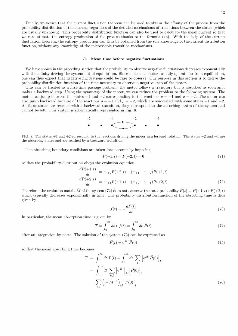
We have shown in the preceding section that the probability to observe negative fluctuations decreases exponentiallywith the affinity driving the system out-of-equilibrium. Since molecular motors usually operate far from equilibrium,one can thus expect that negative fluctuations could be rare to observe. Our purpose in this section is to derive theprobability distribution function of the time necessary to observe a negative step of the motor.

This can be treated as a first-time passage problem: the motor follows a trajectory but is absorbed as soon as itmakes a backward step. Using the symmetry of the motor, we can reduce the problem to the following system. Themotor can jump between the states +1 and +2 corresponding to the reactions ρ = +1 and ρ = +2. The motor canalso jump backward because of the reactions ρ = −1 and ρ = −2, which are associated with some states −1 and −2.As these states are reached with a backward transition, they correspond to the absorbing states of the system andcannot be left. This system is schematically represented in Fig. 8.

+1 +2−2 −1

FIG. 8: The states +1 and +2 correspond to the reactions driving the motor in a forward rotation. The states −2 and −1 arethe absorbing states and are reached by a backward transition.

The absorbing boundary conditions are taken into account by imposing

P (−1, t) = P (−2, t) = 0 (71)

so that the probability distribution obeys the evolution equation

dP (+1, t)dt

= w+2P (+2, t)− (w+1 + w−2)P (+1, t)

dP (+2, t)dt

= w+1P (+1, t)− (w+2 + w−1)P (+2, t) (72)

Therefore, the evolution matrix M of the system (72) does not conserve the total probability P (t) ≡ P (+1, t)+P (+2, t)which typically decreases exponentially in time. The probability distribution function of the absorbing time is thusgiven by

f(t) = −dP (t)dt

(73)

In particular, the mean absorption time is given by

T =∫ ∞

0

dt t f(t) =∫ ∞

0

dt P (t) (74)

after an integration by parts. The solution of the system (72) can be expressed as

~P (t) = eMt ~P (0) (75)

so that the mean absorbing time becomes

T =∫ ∞

0

dt P (t) =∫ ∞

0

dt∑

k

[eMt ~P (0)

]k

=∫ ∞

0

dt∑k,l

[eMt

]kl

[~P (0)

]l

=∑k,l

(− M−1

)kl

[~P (0)

]l

(76)

14

Calculating the inverse matrix M−1

M−1 = − 1det M

(w+2 + w−1 w+2

w+1 w+1 + w−2

)(77)

where det M = (w+1 +w−2)(w+2 +w−1)−w+1w+2, and using the initial conditions P (+i, 0) = LPst(i) correspondingto the stationary state, one finds that the mean time before observing a backward step is given by

T =(w−1 + w+2)(w+1 + w+2 + w−2) + (w−2 + w+1)(w+1 + w+2 + w−1)

(w+1 + w+2 + w−1 + w−2)(w+1w−1 + w+2w−2 + w−1w−2)(78)

In the limit case where w+1, w+2 � w−1, w−2, the mean waiting time becomes

T ' w+1 + w+2

w+1w−1 + w+2w−2(79)

This mean waiting time is depicted in Fig. 9 for the same values of the transition rates as in Figs. 2 and 7.Similarly, one can obtain the probability distribution and all its moments 〈tn〉 because the exponential of the

evolution matrix M can be calculated exactly.

−30 −20 −10 0

A

0

0.5

1

1.5

2

2.5

3

3.5

T

302010

FIG. 9: Mean waiting time T before a negative fluctuation in the six-state model (L = 3). The transition rates take the valuesw+1 = 2, w+2 = 4, w−1 = 1, and w−2 is used as the dependent parameter.

Moreover, one can evaluate the probability that a trajectory will ever reach a total displacement of −1 step. Thisgives the approximate fraction of the trajectories required in order to be able to observe the negative events consideredin the fluctuation relation (64). This is different from the previous consideration where we have been interested in thenegative fluctuations regardless of the total displacement. This probability can be obtained by considering a randomwalk where the sites correspond to the total displacement made by the motor. The initial condition corresponds to anull displacement, and we must consider the two cases where the motor starts from a site of type σ = 1 or from a siteσ = 2, weighted with their respective probabilities. A well-known result in the theory of Markovian random walks(see for instance Ref. [32]) gives the probability which is given by

P =w−1 + w+2

w+1 + w+2 + w−1 + w−2

F (w−2/w+1)1 + F (w−2/w+1)

+w+1 + w−2

w+1 + w+2 + w−1 + w−2

F (w−1/w+2)1 + F (w−1/w+2)

(80)

where

F (x) =x + e−A/L

1− e−A/L(81)

if A > 0. For A ≤ 0, this probability is equal to unity, P = 1, because the mean motion is backward. This probabilityis depicted in Fig. 10 for the same values of the transition rates as in Figs. 2 and 7. These results suggest thatthe fluctuation theorem becomes more and more evident if the system is close to equilibrium and that the randombackward rotations of the motor become rare away from the equilibrium.

15

A

0

0.2

0.4

0.6

0.8

1

1.2

P

−10 0 302010

FIG. 10: Probability P that a trajectory ever reaches a total displacement of −1 step in the six-state model (L = 3). Thetransition rates take the values w+1 = 2, w+2 = 4, w−1 = 1, and w−2 is used as the dependent parameter.

IV. THE F1 MOLECULAR MOTOR

In this section, we apply the discrete-state model described here above to the F1 motor studied by Kinosita andcoworkers in Ref. [19]. The F1 protein complex is composed of three large α- and β-subunits circularly arrangedaround a smaller γ subunit. The three β-subunits are the reactives sites for the hydrolysis of ATP, while the γ subunitplays the role of rotation shaft to which a bead of 40 nm-diameter is glued. The mechanism of rotational catalysis wasproposed by Boyer using a bi-site activation [20]. Nevertheless, experimental data cannot distinguish for the momentbetween the bi-site and three-site activations. The observation [19] clearly shows that the rotation takes place insix steps: ATP binding induces a rotation of about 90◦ followed by the release of ADP and Pi with a rotation ofabout 30◦. Therefore, the hydrolysis of one ATP corresponds to a rotation by 120◦ and a revolution of 360◦ to threesequential ATP hydrolysis in the three β-subunits. The six successive states of the hydrolytic motor M = F1 can thusbe specified by the angle θ of the shaft and the occupancy of the sites of the three β-subunits as

M1 = M[θ = 0, (ADP + Pi, ∅, x)

]M2 = M

[θ =

π

2, (ADP + Pi, ATP, x)

]

M3 = M[θ =

2π

3, (∅, ADP + Pi, x)

]M4 = M

[θ =

5π

6, (x, ADP + Pi, ATP)

](82)

M5 = M[θ =

4π

3, (x, ∅, ADP + Pi)

]M6 = M

[θ =

11π

6, (ATP, x, ADP + Pi)

]where x stands either for ∅ or ADP for the bi- or three-site mechanism. If the site is empty, the F1 complex jumps tothe following state with the rate k+1[ATP], and with the rate k+2 if the site is occupied. The backward transitionsbeing possible, the complex can jump to the preceding state with the rate k−1 if the site is occupied and the ratek−2[ADP][Pi] if it is empty. This process can be summarized by the following reaction scheme

ATP + Mσ

k+1k−1

Mσ+1

k+2k−2

Mσ+2 + ADP + Pi (σ = 1, 3, 5) (83)

with a cyclic ordering M7 ≡ M1. This is the model (27) with L = 3 with the transition rates

w+1 ≡ k+1[ATP]w−1 ≡ k−1

w+2 ≡ k+2

w−2 ≡ k−2[ADP][Pi] (84)

The graph of this six-state model is depicted in Fig. 11. The three-fold symmetry of the F1-ATPase is taken intoaccount in the model by the symmetry of the transition rates.

16

.

6

1 5

.

4

3

2.

.

.

.

FIG. 11: Graph associated with the six-state model.

The standard free enthalpy of hydrolysis is equal to

∆G0 = G0ATP −G0

ADP −G0Pi

= 50 pN nm (85)

The temperature of the experiment of Ref. [19] is 23◦ Celsius so that the equilibrium concentrations of the reactantand products obey

[ATP]eq[ADP]eq[Pi]eq

=k−1k−2

k+1k+2= e−∆G0/kBT = 4.89 10−6 M−1 (86)

which is a constraint on the reaction constants from equilibrium thermodynamics. We notice that, under physiologicalconditions, the concentrations are about [ATP] ' 10−3 M, [ADP] ' 10−4 M, and [Pi] ' 10−3 M, so that ATP is inlarge excess with respect to its equilibrium concentration [ATP]eq ' 4.89 10−13 M, which shows that the system istypically very far from equilibrium.

The reaction constants k±ρ can be determined from the experimental data [22]. In the absence of the products, therotation velocity is observed to follow a Michaelis-Menten kinetics in agreement with Eq. (36) of the model:

V =Vmax[ATP]

[ATP] + KM(87)

with the maximum velocity Vmax = k+2/3 = 129±9 revolutions per second and the Michaelis-Menten constant KM =(k+2 + k−1)/k+1 = 15 ± 2 µM. Furthermore, the dependence of the rotation velocity on the product concentrationscan be used to obtain that k−2/k+1 = 13.7±0.4 M−1 [22]. Thermodynamic equilibrium (86) provides the last relationso that the reaction constants are thus given by

k+1 = (2.6± 0.5) 107 M−1 s−1

k−1 = (138± 34) 10−6 s−1

k+2 = (387± 27) s−1

k−2 = (3.5± 0.8) 108 M−2 s−1 (88)

We observe that these reaction constants range over about twelve orders of magnitude, which is characteristic of astiff stochastic process.

The affinity of the cycle of Fig. 11 is defined as

A ≡ 3 lnk+1k+2[ATP]

k−1k−2[ADP][Pi](89)

which vanishes at equilibrium. Figure 12 shows how the concentration of ATP varies with the affinity for differentconcentrations of the products. We see that the ATP concentration is always very small at equilibrium.

The mean rotation velocity is depicted in Fig. 13 as a function of the affinity (89) for different concentrations ofthe products. We observe that the V -A curve is highly nonlinear as a consequence of the stiffness of the process.Even the vanishing of the mean velocity at the thermodynamic equilibrium A = 0 is not visible in Fig. 13. A zoom iscarried out in the vicinity of equilibrium in Fig. 14 where we observe that indeed the mean velocity vanishes linearlywith the affinity as expected. This linear regime does not extend by more than one decade around the equilibriumconcentration. Typically, the motor is very far from equilibrium and is functioning in the nonlinear regime. This

17

10-10

10-9

10-8

10-7

10-6

10-5

10-4

10-3

10-2

10-1

-20 0 20 40 60 80 100

10-2

10-3

10-4

10-5

10-6

10-7

10-8

10-9

10-10

10-11

10-12

[AT

P]

(M

)

A

[ADP][Pi]

FIG. 12: Concentration of ATP versus the affinity A according to Eq. (89).

-20

0

20

40

60

80

100

120

140

-20 0 20 40 60 80 100

10-2

10-3

10-4

10-5

10-6

10-7

10-8

10-9

10-10

10-11

10-12

V

A

[ADP][Pi]

FIG. 13: Mean rotation velocity V of the F1 motor with a bead of 40 nm-diameter versus the affinity A for different concen-trations [ADP][Pi] of the products.

shows the crucial importance of these nonlinear regimes of nonequilibrium thermodynamics for the understanding ofbiological molecular motors.

Another consequence of the stiffness of the motor is that the diffusion coefficient depicted in Fig. 15 is small relativeto the mean velocity. For most values of the affinity, the ratio of the mean velocity to the diffusion coefficient is aboutV/D ' 6, which is characteristic of a correlated rotation slightly affected by the fluctuations.

Nevertheless, the fluctuation theorem holds even far from equilibrium as we can see in Fig. 16 which depicts thegenerating function (41) of the disspated work. We observe that, indeed, the symmetry (10) of the fluctuation theoremis well satisfied for different concentrations of ATP. Moreover, the fluctuation theorem can be directly verified fromthe statistics of the random steps forward and backward as shown in Fig. 17 where we show that the fluctuationrelation

Prob(St = s) ' Prob(St = −s) e−sA/6 (90)

for the probability Prob(St = s) for s = St steps over a time interval t is indeed satisfied. This verification requiresa statistics proportional to the inverse of the probability given by Eq. (80) which is given in the caption of Fig.17. As seen on Fig. 17, the probability distribution of the displacement takes here a specific form where the odddisplacements are almost never occurring. Indeed, for these values of the concentrations of the chemical species, theprobability to be on odd sites is about 4 order of magnitude lower than the probability to be on even sites. Thesystem almost never stays on odd site and immediately jumps to the next or previous sites.

18

-0.0001

0

0.0001

0.0002

-15 -10 -5 0 5 10

10-2

10-3

10-4

V

A

[ADP][Pi]

FIG. 14: Zoom of Fig. 13 giving the mean rotation velocity V of the F1 motor versus the affinity A around the equilibrium atA = 0 for different concentrations [ADP][Pi] of the products.

-5

0

5

10

15

20

25

-20 0 20 40 60 80 100

10-2

10-3

10-4

10-5

10-6

10-7

10-8

10-9

10-10

10-11

10-12

D

A

[ADP][Pi]

FIG. 15: Diffusion coefficient D of the F1 motor with a bead of 40 nm-diameter versus the affinity A for different concentrations[ADP][Pi] of the products.

As discussed previously, the F1 molecular motor is a stiff process and typically operates in the nonlinear regime witha quality factor close to unity. This means that large fluctuations with negative events rapidly become inobservable.Nevertheless, from the exact solution (60) one can see that the finite time corrections to the fluctuation theoremusually quickly become negligible. Therefore, one can hope to observe the symmetry relation (63) even for systemfurther away from equilibrium if combined with a small enough observation time. In cases where the finite timecorrections are not negligible, one can still calculate the finite time generating function from experimental data andcompare to the exact solution (60) at finite time.

According to Eq. (18), the maximum work which can be done per revolution by the F1 motor is ∆G = 3(µATP −µADP − µPi) = AkBT which can be read in Fig. 12 with kBT = 4.1 pN nm = 4.1 10−11 J.

V. CONCLUSIONS

Molecular motors are functioning at the nanoscale where the fluctuations are important in particular in the chemicalreactions maintaining these nanosystems out of equilibrium. Accordingly, they require a stochastic description to takeinto account the randomness of the reactive events and of the environment. In this description, a central quantity ofinterest is the affinity or thermodynamic force, which is given in terms of the free enthalpy of the chemical reactions.

19

10-6

10-5

10-4

10-3

10-2

10-1

100

101

102

103

0 0.2 0.4 0.6 0.8 1

10-1

10-2

10-3

10-4

10-5

10-6

10-7

10-8

10-9

q(η

)

η

[ATP]

FIG. 16: Generating function q(η) of the dissipated work of the F1 motor with a bead of 40 nm-diameter versus the parameterη for different concentrations of [ATP] and the fixed value [ADP][Pi] = 10−4 M2. We notice that q(η) = 0 at equilibrium where[ATP]eq = 4.89 10−10 M.

0

0.05

0.1

0.15

0.2

0.25

-15 -10 -5 0 5 10 15

Pro

bab

ilit

y

S

FIG. 17: Probability Prob(St = s) (open circles) that the F1 motor performs s = St steps during the time interval t = 104 s

compared with the expression Prob(St = −s) e−sA/6 (crosses) expected from the fluctuation theorem for [ATP] = 6 10−8 Mand [ADP][Pi] = 10−2 M2. The probability (80) is here equal to P = 0.8.

The affinity thus plays a crucial role in the nonequilibrium thermodynamics of molecular motors.In the present paper, we have shown that the affinity can be determined thanks to new large-deviation relationships

known under the name of fluctuation theorems, which we have here applied to molecular motors. The fluctuationtheorems are connected to Jarzynski nonequilibrium work theorem, as discussed in Sec. II. These theorems expressa fundamental symmetry of the molecular fluctuations, which has its origin in the microreversibility. This symmetryconcerns different quantities such as the work dissipated in the irreversible processes, the currents across the system,as well as the displacement for linear motors or the rotation for rotary motors.

Considering a discrete-state stochastic model of molecular motors, we have obtained fluctuation theorems forthese related quantities. The probabilities of their fluctuations obey general relationships which are valid far fromthermodynamic equilibrium and which say that the probabilities of the forward to backward random motions ofthe motor are in a ratio which only depends on the affinity of the process and the number of reactive steps whichhave occurred during some time interval. This provides a method to measure experimentally the affinity of thenonequilibrium process driving the molecular motor. The fluctuation theorem can be expressed for the number ofrevolutions of a rotary motor as well as for the number of steps or the work dissipated during some time interval.

20

These quantities are related to each other by a proportionality factor. The theory also provides the mean current ormean rotation velocity as a function of the affinity, as well as the diffusion coefficient characterizing the fluctuationsaround the mean motion.

We have also studied the time required to observe steps in the direction opposite to the mean motion. The shorterthis time, the higher the statistics of the backward random events needed to use the fluctuation theorem. We have inparticular shown that this time is shorter if the fluctuating quantity is the number of steps instead of the number ofrevolutions.

We have applied these considerations to the F1 motor, which has been experimentally investigated by Kinosita andcoworkers [19]. This molecular motor is a protein complex for the synthesis of ATP in mitochondria. In vitro, a beadcan be glued to its shaft and its rotation can be observed under nonequilibrium conditions fixed by the concentrationof ATP with respect to the concentrations of the products of ATP hydrolysis. The F1 motor is thus an example ofnonequilibrium nanosystem affected by molecular fluctuations. The reaction constants of the discrete-state stochasticmodel can be fitted to the experimental data, which reveals that the process is stiff because the reaction constantsrange over twelve orders of magnitude. Accordingly, the response of the system to the nonequilibrium constraints,i.e., the mean rotation velocity versus the affinity, is a highly nonlinear function. The linear regime only extends overa very small interval of concentrations around chemical equilibrium. Under typical physilogical conditions as well asin the experiments by Kinosita and coworkers [19], the F1 motor functions very far from equilibrium, deep in thenonlinear regime of nonequilibrium thermodynamics. This nonlinearity confers to the rotational motion a robustnesswhich does not exist near equilibrium. This robustness can be characterized by the quality factor of the motor, whichis given in terms of the ratio of the mean rotation velocity over the diffusion coefficient. In the nonlinear regime, thequality factor reaches a value close to unity meaning that the successive rotations are statistically correlated and thusremain essentially unaffected by the molecular fluctuations. Nevertheless, we can show that the fluctuation theorem issatisfied close and far from equilibrium, in both the linear and nonlinear regimes. The fluctuation theorem here saysthat the ratio of the probability of a forward rotation of the shaft to the probability of a backward rotation determinesthe affinity of the process. This provides a method to measure experimentally this affinity which is the free enthalpyof the chemical reaction of hydrolysis. The fluctuation theorem can therefore be used to obtain key information onthe nonequilibrium thermodynamics of molecular motors.

Acknowledgments. The authors thank Professor G. Nicolis for support and encouragement in this research.D. Andrieux is grateful to the F. N. R. S. Belgium for financial support. This research is financially supported by the“Communaute francaise de Belgique” (contract “Actions de Recherche Concertees” No. 04/09-312) and the NationalFund for Scientific Research (F. N. R. S. Belgium, contract F. R. F. C. No. 2.4577.04).

[1] B. Alberts, D. Bray, A. Johnson, J. Lewis, M. Raff, K. Roberts, and P. Walter, Essential Cell Biology (Garland Publishing,New York, 1998).

[2] T. De Donder and P. Van Rysselberghe, Affinity (Stanford University Press, Menlo Park CA, 1936).[3] P. Gaspard, J. Chem. Phys. 120, 8898 (2004).[4] D. Andrieux and P. Gaspard, J. Chem. Phys. 121, 6167 (2004).[5] D. Andrieux and P. Gaspard, Fluctuation theorem for currents and Schnakenberg network theory, Preprint cond-

mat/0512254.[6] D. Andrieux and P. Gaspard, J. Stat. Mech. P01011 (2006).[7] D. J. Evans, E. G. D. Cohen, and G. P. Morriss, Phys. Rev. Lett. 71, 2401 (1993).[8] D. J. Evans and D. J. Searles, Phys. Rev. E 50, 1645 (1994).[9] G. Gallavotti and E. G. D. Cohen, Phys. Rev. Lett. 74, 2694 (1995).

[10] J. Kurchan, J. Phys. A: Math. Gen. 31, 3719 (1998).[11] J. L. Lebowitz and H. Spohn, J. Stat. Phys. 95, 333 (1999).[12] C. Maes, J. Stat. Phys. 95, 367 (1999).[13] G. E. Crooks, Phys. Rev. E 60, 2721 (1999).[14] R. van Zon and E. G. D. Cohen, Phys. Rev. Lett. 91, 110601 (2003).[15] T. Elston, H. Wang, and G. Oster, Nature 391, 510 (1998).[16] H. Wang and G. Oster, Nature 396, 279 (1998).[17] G. Oster and H. Wang, Biochimica et Biophysica Acta 1458, 482 (2000).[18] H. Noji, R. Yasuda, M. Yoshida, and K. Kinosita, Nature 386, 299 (1997).[19] R. Yasuda, H. Noji, M. Yoshida, K. Kinosita, and H. Itoh, Nature 410, 898 (2001).[20] P. D. Boyer, FEBS Letters 512, 29 (2002).[21] Y. Sowa, A. D. Rowe, M. C. Leake, T. Yakushi, M. Homma, A. Ishijima, and R. M. Berry, Nature 437, 916 (2005).[22] E. Gerritsma and P. Gaspard, in preparation.[23] G. Nicolis and I. Prigogine, Self-Organization in Nonequilibrium Systems (Wiley, New York, 1977).

21

[24] C. Jarzynski, Phys. Rev. Lett. 78, 2690 (1997).[25] U. Seifert, Europhys. Lett. 70, 36 (2005).[26] J. Schnakenberg, Rev. Mod. Phys. 48, 571 (1976).[27] Luo Jiu-li, C. Van den Broeck, and G. Nicolis, Z. Phys. B - Condensed Matter 56 (1984) 165.[28] L. Onsager, Phys. Rev. 37, 405 (1931).[29] M. S. Green, J. Chem. Phys. 20 1281 (1952); 22, 398 (1954).[30] R. Kubo, J. Phys. Soc. Jpn. 12 570 (1957).[31] P. Dimroth, H. Wang, M. Grabe, and G. Oster, Proc. Natl. Acad. Sci. USA 96, 4924 (1999).[32] S. Karlin and H. M. Taylor, A First Course in Stochastic Processes, 2nd Edition (Academic Press, New York, 1975).