Embed Size (px)
Citation preview
arX
iv:1
004.
1995
v3 [
mat
h.PR
] 6
Mar
201
2
The Annals of Applied Probability
2012, Vol. 22, No. 1, 70–127DOI: 10.1214/11-AAP759c© Institute of Mathematical Statistics, 2012
SWITCHED NETWORKS WITH MAXIMUM WEIGHT POLICIES:FLUID APPROXIMATION AND MULTIPLICATIVE STATE SPACE
COLLAPSE
By Devavrat Shah1 and Damon Wischik2
Massachusetts Institute of Technology and University College London
We consider a queueing network in which there are constraintson which queues may be served simultaneously; such networks maybe used to model input-queued switches and wireless networks. Thescheduling policy for such a network specifies which queues to serve atany point in time. We consider a family of scheduling policies, relatedto the maximum-weight policy of Tassiulas and Ephremides [IEEETrans. Automat. Control 37 (1992) 1936–1948], for single-hop andmultihop networks. We specify a fluid model and show that fluid-scaled performance processes can be approximated by fluid modelsolutions. We study the behavior of fluid model solutions under criti-cal load, and characterize invariant states as those states which solvea certain network-wide optimization problem. We use fluid model re-sults to prove multiplicative state space collapse. A notable featureof our results is that they do not assume complete resource pooling.
1. Introduction. A switched network consists of a collection of queues,operating in discrete time. In each time slot, queues are offered service ac-cording to a service schedule chosen from a specified finite set. For exam-ple, in a three-queue system, the set of allowed schedules might consist of“Serve 3 units of work each from queues A and B” and “Serve 1 unit ofwork each from queues A and C, and 2 units from queue B.” The rule forchoosing a schedule is called the scheduling policy. New work may arrive ineach time slot; let each queue have a dedicated exogenous arrival process,with specified mean arrival rates. Once work is served, it may either rejoinone of the queues or leave the network.
Received August 2007; revised January 2011.1Supported by NSF CAREER CNS-0546590.2Supported by a Royal Society university research fellowship. Collaboration supported
by the British Council Researcher Exchange program.AMS 2000 subject classifications. 60K25, 60K30, 90B36.Key words and phrases. Switched network, maximum weight scheduling, fluid models,
state space collapse, heavy traffic, diffusion approximation.
This is an electronic reprint of the original article published by theInstitute of Mathematical Statistics in The Annals of Applied Probability,2012, Vol. 22, No. 1, 70–127. This reprint differs from the original in paginationand typographic detail.
1
2 D. SHAH AND D. WISCHIK
Switched networks are special cases of what Harrison [12, 13] calls “stochas-tic processing networks.” We believe that switched networks are generalenough to model a variety of interesting applications. For example, theyhave been used to model input-queued switches, the devices at the heartof high-end internet routers, whose underlying silicon architecture imposesconstraints on which traffic streams can be transmitted simultaneously [8].They have also been used to model a multi-hop wireless network in whichinterference limits the amount of service that can be given to each host [28].
The main result of this paper is Theorem 7.1, which proves multiplicativestate space collapse (as defined in Bramson [3]) for a switched network run-ning a generalized version of the maximum-weight scheduling policy of Tas-siulas and Ephremides [28], in the diffusion (or heavy traffic) limit. Whereasprevious works on switched networks and stochastic processing networks inthe diffusion limit [6, 7, 27] have assumed the “complete resource pooling”condition, which roughly means that there is a single bottleneck cut con-straint, we do not make this assumption. Section 3 discusses further therelated work and our reasons for being interested in the case without com-plete resource pooling.
To prove multiplicative state space collapse we follow the general methodlaid out by Bramson [3]. In Section 2 we specify a stochastic switched net-work model and describe the generalized maximum-weight policy. In Sec-tion 4 we specify a fluid model and prove that fluid-scaled performanceprocesses of the switched network are approximated by solutions of thisfluid model. Sections 5 and 6 give properties of the solutions of the fluidmodel for single-hop and multi-hop networks, respectively. Specifically, fornonoverloaded fluid model solutions, we characterize the invariant statesand prove that fluid model solutions converge towards the set of invariantstates. In Section 7 we use these properties to prove multiplicative statespace collapse.
We use the cluster-point method of Bramson [3] to prove the fluid modelapproximation in Section 4, rather than following an approach based onweak convergence. The former yields uniform bounds on the error of fluidmodel approximations, and these uniform bounds are needed in provingmultiplicative state space collapse. However, the assumptions we make onthe arrival process are not the same as those of Bramson [3].
In Section 8 we give results concerning the fluid model behavior of a gen-eral single-hop switched network in critical load, and the set of invariantstates for the input-queued switch, under a condition that we call “completeloading.” Motivated by these results, we define a scheduling policy which weconjecture is optimal in the diffusion limit.
Notation. Let N be the set of natural numbers {1,2, . . .}, let Z+ = {0,1,2, . . .}, let R be the set of real numbers and let R+ = {x ∈R :x≥ 0}. Let 1{·}
NETWORK SCHEDULING 3
be the indicator function, where 1true = 1 and 1false = 0. Let x∧y =min(x, y),x∨y =max(x, y) and [x]+ = x∨0. When x is a vector, the maximum is takencomponentwise.
We will reserve bold letters for vectors in RN , where N is the number
of queues, for example, x = [xn]1≤n≤N . Superscripts on vectors are usedto denote labels, not exponents, except where otherwise noted; thus, forexample, (x0,x1,x2) refers to three arbitrary vectors. Let 0 be the vectorof all 0s, and 1 be the vector of all 1s. Use the norm |x| =maxn |xn|. Forvectors u and v and functions f :R→R, let
u · v=N∑
n=1
unvn, uv= [unvn]1≤n≤N and f(u) = [f(un)]1≤n≤N ,
and let matrix multiplication take precedence over dot product so that
u ·Av=N∑
n=1
un
(
N∑
m=1
Anmvm
)
.
Let AT be the transpose of matrix A. For a set S ⊂ RN , denote its convex
hull by 〈S〉.For a fixed T > 0, and I ∈N, let CI(T ) be the set of continuous functions
[0, T ]→RI , where RI is equipped with the norm |x|=maxi|xi|. Equip CI(T )
with the norm
‖f‖= supt∈[0,T ]
|f(t)|.
Let d(f, g) = ‖f − g‖ be the metric induced by this norm. For E ⊂ CI(T )and f ∈CI(T ), let d(f,E) = inf{d(f, g) :g ∈E}. Define the modulus of con-tinuity mcδ(·) by
mcδ(f) = sup|s−t|<δ
|f(s)− f(t)|,
where s, t ∈ [0, T ]. Since [0, T ] is compact, each f ∈CI(T ) is uniformly con-tinuous, therefore mcδ(f)→ 0 as δ→ 0.
2. Switched network model. We now introduce the switched networkmodel. Section 2.1 describes the general system model, Section 2.2 specifiesthe class of scheduling policies we are interested in and Section 2.3 lists theprobabilistic assumptions about the arrival process that are needed for themain theorems.
2.1. Queueing dynamics. Consider a collection of N queues. Let time bediscrete, indexed by τ ∈ {0,1, . . .}. Let Qn(τ) be the amount of work in queuen ∈ {1, . . . ,N} at time slot τ . Following our general notation for vectors, wewrite Q(τ) for [Qn(τ)]1≤n≤N . The initial queue sizes are Q(0). Let An(τ) bethe total amount of work arriving to queue n, and Bn(τ) be the cumulativepotential service to queue n, up to time τ , with A(0) =B(0) = 0.
4 D. SHAH AND D. WISCHIK
We first define the queueing dynamics for a single-hop switched network.Defining dA(τ) =A(τ +1)−A(τ) and dB(τ) =B(τ +1)−B(τ), the basicLindley recursion that we will consider is
Q(τ + 1) = [Q(τ)− dB(τ)]+ + dA(τ),(1)
where the [·]+ is taken componentwise. The fundamental “switched network”constraint is that there is some finite set S ⊂R
N+ such that
dB(τ) ∈ S for all τ .(2)
We will refer to π ∈ S as a schedule and S as the set of allowed schedules.In the applications in this paper, the schedule is chosen based on currentqueue sizes, which is why it is natural to write the basic Lindley recursionas (1) rather than the more standard [Q(τ) + dA(τ)− dB(τ)]+.
For the analyses in this paper it is useful to keep track of two otherquantities. Let Yn(τ) be the cumulative amount of idling at queue n, definedby Y(0) = 0 and
dY(τ) = [dB(τ)−Q(τ)]+,(3)
where dY(τ) =Y(τ +1)−Y(τ). Then (1) can be rewritten
Q(τ) =Q(0) +A(τ)−B(τ) +Y(τ).(4)
Also, let Sπ(τ) be the cumulative time spent on schedule π up to time τ ,so that
B(τ) =∑
π∈S
Sπ(τ)π.(5)
For a multi-hop switched network, let R ∈ {0,1}N×N be the routing ma-trix, Rmn = 1 if work served from queue m is sent to queue n and Rmn = 0otherwise; if Rmn = 0 for all n, then work served from queue m departs thenetwork. For each m we require Rmn = 1 for at most one n. (Tassiulas andEphremides [28] described a network model with routing choice, whereaswe have restricted ourselves to fixed routing for the sake of simplicity.) Thescheduling constraint (2) is as before, the definition of idling (3) is as beforeand the queueing dynamics are now defined by
Qn(τ+1) =Qn(τ)+dAn(τ)−(dBn(τ)−dYn(τ))+∑
m
Rmn(dBm(τ)−dYm(τ)).
Equivalently,
Q(τ) =Q(0) +A(τ)− (I −RT)(B(τ)−Y(τ)).(6)
Note that A includes only exogenous arrivals to the network, not internallyrouted traffic. We will assume that routing is acyclic, that is, that workserved from some queue n never returns to queue n. For example, BorderGateway Protocol (BGP) utilized for routing in the internet is designed
to be acyclic [31]. This implies that the inverse ~R = (I −RT)−1 exists; by
considering the expansion ~R = I +RT + (RT)2 + · · · it is clear that ~Rmn ∈
NETWORK SCHEDULING 5
{0,1} for all m, n and that ~Rmn = 1 if work injected at queue n eventually
passes through m, and ~Rmn = 0 otherwise. When R= 0 we obtain a single-hop switched network.
A straightforward bound we shall need is
Qn(τ)≤Qn(τ′) +An(τ)−An(τ
′) +∑
m
Rmn(Bm(τ)−Bm(τ ′))(7)
for τ ′ ≤ τ .
2.2. Scheduling policy. A policy that decides which schedule to chooseat each time slot τ ∈ Z+ is called a scheduling policy. In this paper we willbe interested in the max-weight scheduling policy, introduced by Tassiulasand Ephremides [28]. We will refer to it as MW.
2.2.1. Max-weight policy for single-hop network. We describe the policyfirst for a single-hop network. Let Q(τ) be the vector of queue sizes at time τ .Define the weight of a schedule π ∈ S to be π ·Q(τ). The MW policy thenchooses3 for time slot τ a schedule dB(τ) with the greatest weight,
dB(τ) ∈ argmaxπ∈S
π ·Q(τ).(8)
This policy can be generalized to choose a schedule which maximizes π ·Q(τ)α, where the exponent is taken componentwise for some α> 0; call thisthe MW-α policy. More generally, one could choose a schedule such that
dB(τ) ∈ argmaxπ∈S
π · f(Q(τ))(9)
for some function f :R+ → R+; call this the MW-f policy. It is assumedthat f satisfies the following scale-invariance property:
Assumption 2.1. Assume f is differentiable and strictly increasing withf(0) = 0. Assume also that for any q ∈ R
N+ and π ∈ S , with m(q) =
maxρ∈S ρ · f(q),π · f(q) =m(q) =⇒ π · f(κq) =m(κq) for all κ ∈R+.
This is satisfied by f(x) = xα, α > 0, but it is not satisfied, for example,for an input-queued switch with f(x) = log(1 + x).
3There may be several schedules which jointly have the greatest weight. To be concrete,we might specify some fixed numbering of schedules and choose the highest-numberedmaximum-weight schedule. Alternatively, we might treat MW not as a policy per se butas a constraint on the set of allowed sample paths. For example, in a stochastic setting,we might allow dB(τ ) to be a random variable, measurable with respect to the underlyingprobability space, satisfying (8) for every randomness. This permits “break ties at ran-dom.” For the analyses in this paper, it makes no difference which of these two options isused.
6 D. SHAH AND D. WISCHIK
2.2.2. Max-weight policy for multi-hop network. Now we define the multi-hop version of the MW-f scheduling policy. This policy chooses a sched-ule dB(τ) at time τ such that
dB(τ) ∈ argmaxπ∈S
π · (I −R)f(Q(τ)).
Recall that matrix multiplication takes precedence over the · operator, sothe argmax is of π · {(I −R)f(Q(τ))}; note also that
[Rf(Q)]n =∑
m
Rnmf(Qm) = f([RQ]n),
where [RQ]n is the queue size at the first queue downstream of n (or 0 ifthere is no queue downstream). Thus
[(I −R)f(Q)]n = f(Qn)− f([RQ]n).(10)
The difference f(Qn)− f([RQ]n) is interpreted as the pressure to send workfrom queue n to the queue downstream of n; if the downstream queue hasmore work in it than the upstream queue, then there is no pressure to sendwork downstream. For this reason, it is also known as backpressure policy.
As before we will assume that f satisfies a scale-invariance property, themulti-hop equivalent of Assumption 2.1:
Assumption 2.2. Assume f is differentiable and strictly increasing withf(0) = 0. Assume also that for any q ∈ R
N+ and π ∈ S , with m(q) =
maxρ∈S ρ · (I −R)f(q),
π ·(I−R)f(q) =m(q) =⇒ π ·(I−R)f(κq) =m(κq) for all κ ∈R+.
We further require that the scheduler always have the option of not send-ing work downstream at any individual queue. Our Lyapunov function, andindeed our whole fluid analysis in Section 6, rely on this assumption.
Assumption 2.3. For the multi-hop setting, assume that S satisfies thefollowing: if π ∈ S is an allowed schedule, and ρ ∈R
N+ is some other vector
with ρn ∈ {0, πn} for all n, then ρ ∈ S .
In the rest of this paper, whenever we refer to a network running theMW-f back-pressure policy, we mean that Assumptions 2.2 and 2.3 aresatisfied.
2.3. Stochastic model. Some of the results in this paper are about fluid-scaled processes, and others are about multiplicative state space collapse inthe diffusion scaling, and the different results make different assumptionsabout the arrival process.
Assumption 2.4 (Assumptions for the fluid scale). Let A(·) be a ran-dom process with stationary increments. Assume it has a well-defined mean
NETWORK SCHEDULING 7
arrival rate vector λ, that is, assume limτ→∞An(τ)/τ exists almost surelyand is deterministic for every queue 1≤ n≤N , and define
λn = limτ→∞
1
τAn(τ).(11)
Assume there is a sequence of deviation terms δr ∈ R+, r ∈ N, such thatδr → 0 as r→∞ and
P
(
supτ≤r
1
r|A(τ)−λτ | ≥ δr
)
→ 0 as r→∞.
Assumption 2.5 (Assumptions for multiplicative state space collapse).Let Ar(·) be a sequence of random processes indexed by r ∈N. For each r,assume that Ar has stationary increments, and a well-defined mean arrivalrate vector λr, and that there is some limiting arrival rate vector λ such that
λr → λ as r→∞.
Assume there is a sequence of deviation terms δz ∈ R+, z ∈ N, such thatδz → 0 as z →∞ and
z(log z)2P
(
supτ≤z
1
z|Ar(τ)− λrτ | ≥ δz
)
→ 0 as z→∞, uniformly in r.
If the arrival process is the same for all r, say Ar = A where A hasa well-defined mean arrival rate vector, then Assumption 2.5 reduces to
P
(
supτ≤r
1
r|A(τ)−λτ | ≥ δr
)
= o
(
1
r(log r)2
)
,(12)
and it implies Assumption 2.4. For any arrival process with i.i.d. incrementsthat are uniformly bounded, that is, such that there is an Amax for which
An(τ + 1)−An(τ) ∈ [0,Amax] for all n, τ ,
equation (12) holds with δr = C√log r/
√r, with choice of an appropriate
constant C that depends on Amax, by an application of concentration in-equality by Azuma [2] and Hoeffding [14]. More generally, it holds whenthe increments are not uniformly bounded but instead satisfy a reasonablemoment bound. For example, an application of Doob’s maximal inequal-ity [10] with bounded fourth moment and δr = r−1/6 yields a stronger resultthan (12); this can be used to show that a Poisson process satisfies thatequation. Furthermore (12) holds for a much larger class of stationary ar-rival processes beyond processes with i.i.d. increments, for example, Markovmodulated processes (see Dembo and Zeitouni [9]).
2.4. Motivating example. An internet router has several input ports andoutput ports. A data transmission cable is attached to each of these ports.Packets arrive at the input ports. The function of the router is to workout which output port each packet should go to, and to transfer packets to
8 D. SHAH AND D. WISCHIK
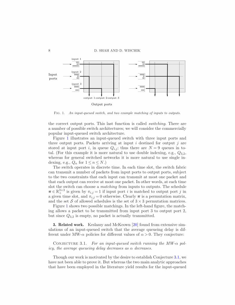
Fig. 1. An input-queued switch, and two example matching of inputs to outputs.
the correct output ports. This last function is called switching. There area number of possible switch architectures; we will consider the commerciallypopular input-queued switch architecture.
Figure 1 illustrates an input-queued switch with three input ports andthree output ports. Packets arriving at input i destined for output j arestored at input port i, in queue Qi,j ; thus there are N = 9 queues in to-tal. (For this example it is more natural to use double indexing, e.g., Q3,2,whereas for general switched networks it is more natural to use single in-dexing, e.g., Qn for 1≤ n≤N .)
The switch operates in discrete time. In each time slot, the switch fabriccan transmit a number of packets from input ports to output ports, subjectto the two constraints that each input can transmit at most one packet andthat each output can receive at most one packet. In other words, at each timeslot the switch can choose a matching from inputs to outputs. The scheduleπ ∈R
3×3+ is given by πi,j = 1 if input port i is matched to output port j in
a given time slot, and πi,j = 0 otherwise. Clearly π is a permutation matrix,and the set S of allowed schedules is the set of 3× 3 permutation matrices.
Figure 1 shows two possible matchings. In the left-hand figure, the match-ing allows a packet to be transmitted from input port 3 to output port 2,but since Q3,2 is empty, no packet is actually transmitted.
3. Related work. Keslassy and McKeown [20] found from extensive sim-ulations of an input-queued switch that the average queueing delay is dif-ferent under MW-α policies for different values of α> 0. They conjecture:
Conjecture 3.1. For an input-queued switch running the MW-α pol-icy, the average queueing delay decreases as α decreases.
Though our work is motivated by the desire to establish Conjecture 3.1, wehave not been able to prove it. But whereas the two main analytic approachesthat have been employed in the literature yield results for the input-queued
NETWORK SCHEDULING 9
switch that are insensitive to α, our result about multiplicative state spacecollapse is sensitive, as shown in Section 8. We speculate that our resultmight eventually form part of a proof of the conjecture.
The two main analytic approaches that have been employed in the liter-ature are stability analysis and heavy traffic analysis. In stability analysis,one calculates the set of arrival rates for which a policy is stable (in thesense of [1, 8, 20, 24, 25, 28]). All the prior work in this context leads to theconclusion that MW-α has the optimal stability region, regardless of α.
In heavy traffic analysis, one looks at queue size behavior under a dif-fusion (or heavy traffic) scaling. This regime was first described by King-man [21]; since then a substantial body of theory has developed, and moderntreatments can be found in [3, 11, 29, 30]. Stolyar has studied MW-α fora generalized switch model in the diffusion scaling, and obtained a completecharacterization of the diffusion approximation for the queue size process,under a condition known as “complete resource pooling.” This condition ef-fectively requires that a clever scheduling policy be able to balance workbetween all the heavily loaded queues. Stolyar [27] showed in a remarkablepaper that the limiting queue size lives in a one-dimensional state space.Operationally, this means that all one needs to keep track of is the one-dimensional total amount of work in the system (called the workload), andat any point in time one can assume that the individual queues have all beenbalanced. Dai and Lin [6, 7] have established that similar result holds in themore general setting of a stochastic processing network.
Under the complete resource pooling condition, the results in [6, 7, 27]imply that the performance of MW-α in an input-queued switch is alwaysoptimal (in the diffusion scaling) regardless of the value of α> 0. Thereforethese results do not help in addressing Conjecture 3.1. This is our motivationfor studying switched networks in the absence of complete resource pooling.Technically, the lifting map for a critically-loaded input-queued switch isdegenerate and insensitive to α under complete resource pooling, but it issensitive to α otherwise.
We prove multiplicative state space collapse, following the method ofBramson [3]. The complement of Bramson’s work is by Williams [30], andconsists of proving a diffusion approximation, using an appropriate invari-ance principle along with the multiplicative state space collapse. We do notcarry out this complementary aspect. Stolyar [27] and Dai and Lin [6, 7]have proved the diffusion approximation under the complete resource pool-ing condition, and Kang and Williams [17] have made progress toward itin the case without complete resource pooling, for an input-queued switchunder the MW-1 policy.
Whereas in heavy traffic models of other systems [3, 11, 27, 30] the lift-ing map from workloads to queue sizes is linear, we find instead that it isnonlinear—in fact it can be expressed as the solution to an optimizationproblem. The objective function of the problem is a natural generalization
10 D. SHAH AND D. WISCHIK
of the Lyapunov function introduced by Tassiulas and Ephremides [28] forproving stability of the MW-1 policy; the constraints of the problem areclosely linked to the canonical representation of workload identified by Har-rison [12]. The objective function for MW-α depends on α, and this hintsthat the performance measures might also depend on α.
Finally, we take note of two related results. First, in [26] we have reportedsome results about a critically loaded input-queued switch without a com-plete resource pooling condition. Second, a sequence of works by Kelly andWilliams [19] and Kang et al. [16] has resulted in a diffusion approximationfor a bandwidth sharing network model operating under proportionally fairrate allocation, assuming a technical “local traffic” condition, but withoutassuming complete resource pooling. They show that the resulting diffusionapproximation model has a product form stationary distribution.
4. The fluid approximation. This section introduces the fluid model andestablishes it as an approximation to a fluid-scaled descriptor of the switchednetwork. Intuitively, the fluid model describes the dynamics of the systemat the “rate” level rather than at finer granularity. The reader is referredto a recent monography by Bramson [4] and lecture notes by Dai [5] fora detailed account of fluid approximation for multiclass queueing networks.In Section 4.1 we specify the fluid model, in Section 4.2 we state the mainresult and in Section 4.3 we prove it.
4.1. Definition of fluid model. Let time be measured by t ∈ [0, T ] forsome fixed T > 0. Let q, a and y all be continuous functions mapping [0, T ]into R
N+ , and let s = (sπ)π∈S be a collection of continuous functions map-
ping [0, T ] into R+. Let x(·) = (q(·),a(·),y(·), s(·)). This lies in CI(T ) whereI = 3N + |S|. The definition below requires these functions to be absolutelycontinuous; such functions are differentiable almost everywhere, and the timeinstants where they are differentiable are called “regular times.” Any equa-tions we write involving derivatives are taken to apply only at regular times.
Definition 4.1 (Fluid model solution for single-hop network). Let f :R+ →R+ satisfy Assumption 2.1. Say that x(·) is a fluid model solution fora single-hop switched network with arrival rate λ ∈RN
+ operating under theMW-f policy if it satisfies equations (13)–(20) below. Write FMS for the setof all such x ∈CI(T ). Additionally, define
FMSK = {x ∈ FMS: |q(0)| ≤K},FMS(q0) = {x ∈ FMS:q(0) = q0}.
The equations are:
q(t) = q(0) + a(t)−∑
π
sπ(t)π + y(t);(13)
NETWORK SCHEDULING 11
a(t) = λt;(14)∑
π∈S
sπ(t) = t;(15)
y(t)≤∑
π∈S
sπ(t)π;(16)
each sπ(·) and yn(·) is increasing (not necessarily strictly increasing);(17)
all the components of x(·) are absolutely continuous;(18)
for regular times t, all n yn(t) = 0 if qn(t)> 0;(19)
for regular times t, all π ∈ S(20)
sπ(t) = 0 if π · f(q(t))<maxρ∈S
ρ · f(q(t)).
Here, q(t) represents the vector of queue sizes at time t, a(t) represents thecumulative arrivals up to time t, y(t) represents the cumulative idleness upto time t and sπ(t) represents the total amount of time spent on schedule πup to time t. The equation in (13) is the continuous analog of (4) combinedwith (5), and the inequality is the analog of the single-hop version of (7).Equation (14) represents an assumption about the arrival process, relatedto (11). Equation (15) says that the scheduling policy must choose someschedule at every timestep. Both (16) and (19) derive from the definition ofidling, (3). Equation (20) is the continuous analog of (9).
Definition 4.2 (Fluid model solution for multi-hop network). Let f :R+ → R+ satisfy Assumption 2.2, and let S satisfy Assumption 2.3. Saythat x(·) is a fluid model solution for a multi-hop switched network operat-ing under the MW-f policy if it satisfies equations (14)–(19), and addition-ally (21) and (22) below. Let FMSm be the set of all such x ∈CI(T ). Also,let FMSmK and FMSm(q0) be defined analogously to the single-hop case.The extra equations are
q(t) = q(0) + a(t)− (I −RT)
(
∑
π
sπ(t)π − y(t)
)
(21)
and
for all regular times t, all π ∈ S(22)
sπ(t) = 0 if π · (I −R)f(q(t))<maxρ∈S
ρ · (I −R)f(q(t)).
When we refer to “fluid model solutions for any scheduling policy,” wemean processes x(·) ∈ CI(T ) satisfying (13) to (19) in the single-hop case,or satisfying (14) to (19) plus (21) in the multi-hop case.
12 D. SHAH AND D. WISCHIK
4.2. Main fluid model result. The development in this section follows thegeneral pattern of Bramson [3]. There is, however, a difference in presenta-tion that is worth noting. The main result of this section, Theorem 4.3,is a general purpose sample path-wise result: it does not make any proba-bilistic claim nor does it depend on any probabilistic assumptions. It can beapplied to a switched network with stochastic arrivals in two ways: to obtaina result about fluid approximations (Corollary 4.4), and to obtain a resultabout multiplicative state space collapse (Section 7).
We start by defining the fluid scaling. Consider a switched network ofthe type described in Section 2.1 running a scheduling policy of the typedescribed in Section 2.2. Write X(τ) = (Q(τ),A(τ),Y(τ), S(τ)), τ ∈ Z+, todenote its sample path. Given a scaling parameter z ≥ 1, define the fluid-scaled sample path x(t) = (q(t), a(t), y(t), s(t)) for t ∈R+ by
q(t) =Q(zt)/z, a(t) =A(zt)/z,
y(t) =Y(zt)/z, sπ(t) = Sπ(zt)/z
after extending the domain of X(·) to R+ by linear interpolation in eachinterval (τ, τ + 1). In this section we are interested in the evolution of x(t)over t ∈ [0, T ] for some fixed T > 0, therefore we take x to lie in CI(T ) withI = 3N + |S|.
The following theorem concerns uniform convergence of a set of fluid-scaled sample paths. Every fluid-scaled sample path is assumed to relateto some (unscaled) switched network, and all the switched networks are as-sumed to have the same network data, that is, the same number of queues N ,the same set of allowed schedules S , the same routing matrix R, and thesame scheduling policy.
The convergence is indexed by a parameter j lying in some totally orderedcountable set. For Corollary 4.4 we will use j ∈N, and for Section 7 we willuse a subset of N×N as the index set. We are purposefully using the symbol jhere as an index, rather than the r used elsewhere, to remind the reader thatthe index set is interpreted differently in different results.
Theorem 4.3. Let X be the set of all possible sample paths for single-hop switched networks with the network data specified above, running theMW-f scheduling policy, where f satisfies Assumption 2.1. Fix K > 0 andλ ∈R
N+ . Let there be sequences εj ∈R+ and λj ∈R
N+ , indexed by j in some
totally ordered countable set, such that
εj → 0 and λj → λ, as j →∞.(23)
Consider a sequence of subsets Gj ⊂ CI(T ) × [1,∞) which satisfy the fol-lowing: for every (x, z) ∈Gj there is some unscaled sample path X ∈ X suchthat x is the fluid-scaled version of X with scaling parameter z (here z is
NETWORK SCHEDULING 13
permitted to be a function of X); and furthermore
inf{z : (x, z) ∈Gj}→∞ as j →∞,(24)
sup(x,z)∈Gj
supt∈[0,T ]
|a(t)−λjt| ≤ εj for all j(25)
and
sup(x,z)∈Gj
|q(0)| ≤K for all j.(26)
Then
sup(x,z)∈Gj
d(x,FMSK)→ 0 as j →∞.(27)
Furthermore, fix q0 ∈RN+ and a sequence ε′j → 0, and assume that the sets Gj
also satisfy
sup(x,z)∈Gj
|q(0)− q0| ≤ ε′j for all j.(28)
Then
sup(x,z)∈Gj
d(x,FMS(q0))→ 0 as j →∞.(29)
Equivalent results to (27) and (29) apply to multi-hop switched networks,with references to FMS replaced by FMSm and the set X modified to referto multi-hop networks running the MW-f scheduling policy where f satisfiesAssumption 2.2 and S satisfies Assumption 2.3.
The above theorem as stated applies to the MW-f scheduling policy, butit is clear from the proof that a corresponding limit result holds, relatingsample paths of any scheduling policy to fluid models defined by equa-tions (13)–(19).
The following corollary is a straightforward application of Theorem 4.3.It specializes the theorem to the case of a single random system X , andthe sequence of fluid-scaled versions indexed by r ∈N where the rth versionuses scaling parameter r. The arrival process is assumed to satisfy certainstochastic assumptions. This corollary is useful when studying the behaviorof a single switched network with random arrivals, over long timescales.
Corollary 4.4. Consider a single-hop switched network as describedin Section 2.1, running the MW-f policy as described in Section 2.2 where fsatisfies Assumption 2.1. Let the arrival process A(·) satisfy Assumption 2.4,and let the initial queue size Q(0) ∈R
N+ be random. For r ∈N, let
qr(t) =Q(rt)/r, ar(t) =A(rt)/r,
yr(t) =Y(rt)/r, srπ(t) = Sπ(rt)/r,
14 D. SHAH AND D. WISCHIK
and let xr(t) = (qr(t), ar(t), yr(t), sr(t)), for t ∈ [0, T ] where T > 0 is somefixed time horizon. Then for any δ > 0
P(d(xr(·),FMS(0))< δ)→ 1 as r→∞.
The same conclusion holds for a multi-hop switched network running theMW-f back-pressure policy where f satisfies Assumption 2.2 and S satisfiesAssumption 2.3, with FMS replaced by FMSm.
Proof. First define the event Er by
Er =
{
supτ≤r
1
r|A(τ)− λτ |< δr and |Q(0)| ≤
√r
}
,
where λ and δr are as in Assumption 2.4. By this we mean that Er is a subsetof the probability sample space, and we write X(·)(ω) etc. for ω ∈ Er toemphasize the dependence on Er.
We will apply Theorem 4.3 with index set j ≡ r ∈ N to the sequence ofsets
Gj ≡Gr = {(xr(·)(ω), r) :ω ∈Er}.In order to apply the theorem we will pick constants as follows. Let K = 1,let λ be as in Assumption 2.4, λj = λ for all j, εj ≡ εr = Tδr where δr isas in Assumption 2.4, q0 = 0 and ε′r = 1/
√r. We now need to verify the
conditions of Theorem 4.3. Equation (23) holds by the choice of λj andby Assumption 2.4. Equation (24) holds automatically by choice of Gj . Tosee that (25) holds, rewrite event Er in terms of the fluid scaled arrivalprocess ar to see
supt∈[0,T ]
|ar(t)(ω)−λt|< Tδr for all r and ω ∈Er,
which implies (25); likewise for (26) and (28). We conclude that (29) holds.It may be rewritten in terms of Er as
supω∈Er
d(xr(·)(ω),FMS(0))→ 0 as r→∞.(30)
We next argue that P(Er)→ 1 as r→∞. The event Er is the intersectionof two events, one concerning arrivals and the other concerning initial queuesize. The probability of the former → 1 as r →∞ by Assumption 2.4. Forthe latter, P(|Q(0)| ≤ √
r)→ 1 as r →∞ since Q(0) is assumed not to beinfinite. Therefore P(Er) → 1. Combining this with (30) gives the desiredresult for single-hop networks. The multi-hop version follows similarly. �
4.3. Proof of Theorem 4.3. We shall present the proof of Theorem 4.3for a single-hop network in detail followed by main ideas required to extendit to multi-hop networks.
NETWORK SCHEDULING 15
4.3.1. Cluster points. Here we are interested in convergence in CI(T ),where I = 3N + |S| and T > 0 is fixed, equipped with the norm ‖ · ‖. Theappropriate concept for proving convergence is cluster points. Consider anymetric space E with metric d and a sequence (E1,E2, . . .) of subsets of E.Say that x ∈ E is a cluster point of the sequence if lim infj→∞ d(x,Ej) = 0where d(x,Ej) = inf{d(x, y) :y ∈Ej}.
Proposition 4.5 [Cluster points in CI(T )]4. Given K > 0, A> 0 anda sequence Bj → 0, let
Kj = {x ∈CI(T ) : |x(0)| ≤K and mcδ(x)≤Aδ +Bj for all δ > 0},and consider a sequence (E1,E2, . . .) of subsets of C
I(T ) for which Ej ⊂Kj .Then supy∈Ej
d(y,CP)→ 0 as j →∞, where CP is the set of cluster points
of (E1,E2, . . .).
4.3.2. Proof of Theorem 4.3. Let Ej = {x : (x, z) ∈Gj}. Lemma 4.6 belowshows that Ej ⊂Kj , with Kj as defined in Proposition 4.5 for appropriateconstants K, A and Bj . By applying that proposition,
supx∈Ej
d(x,CP)→ 0 as j →∞,
where CP is the set of cluster points of the Ej sequence. Lemma 4.7 belowshows that all cluster points of the Ej sequence satisfy the fluid model equa-tions. Every cluster point x must also satisfy |q(0)| ≤K, by (26). Therefore
supx∈Ej
d(x,FMSK)→ 0 as j →∞.
If in addition (28) holds, then every cluster point x must also satisfy q(0) =q0. Therefore
supx∈Ej
d(x,FMS(q0))→ 0 as j →∞.
Lemma 4.6 (Tightness of fluid scaling). Let K and Gj be as in Theo-rem 4.3. Then there exist a constant A> 0 and a sequence Bj → 0 such thatfor every (x, z) ∈Gj , |x(0)| ≤K and
|x(u)− x(t)| ≤A|u− t|+Bj for all 0≤ t, u≤ T .
Proof. Consider (x, z) ∈ Gj , where x = (q, a, y, s). As per the defi-nitions in Section 2.1, the only nonzero component of x(0) is q(0) and|q(0)| ≤ K by choice of Gj , hence |x(0)| ≤ K. For the second inequality,without loss of generality pick any 0 ≤ t < u ≤ T , and let us now look ateach component of |x(u)− x(t)| in turn.
4Taken from Bramson [3], Proposition 4.1.
16 D. SHAH AND D. WISCHIK
For arrivals, let λmax = supj |λj |; this is finite by the assumption that
λj → λ in Theorem 4.3. Then for (x, z) ∈Gj ,
|a(u)− a(t)| ≤ |a(u)− λju|+ |λj(u− t)|+ |a(t)−λjt|≤ 2εj + |λj|(u− t) by (25)
≤ 2εj + λmax(u− t).
For idling, let Smax = maxπ∈S maxn πn. This is the maximum amount ofservice that can be offered to any queue per unit time, and it must be finitesince |S| is finite. Then, based on (3),
|yn(u)− yn(t)| ≤ (u− t)Smax + 2Smax/z
≤ (u− t)Smax + 2Smax/zminj ,
where zminj = inf{z : (x, z) ∈Gj}. For service, let Sπ(·) be the unscaled pro-
cess that corresponds to sπ(·); since Sπ(·) is increasing and since a schedulemust be chosen not more than once every time slot,
|sπ(u)− sπ(t)| ≤1
z(Sπ(⌈zu⌉)−Sπ(⌊zt⌋))≤ (u− t)+ 2/z ≤ (u− t)+ 2/zmin
j .
For queue size, note that (4) carries through to the fluid model scaling, thatis,
q(t) = q(0) + a(t)−∑
π
sπ(t)π + y(t),
thus
|qn(u)− qn(t)|≤ |an(u)− an(t)|+
∑
π
πn|sπ(u)− sπ(t)|+ |yn(u)− yn(t)|
≤ (u− t)(λmax + |S|Smax + Smax) + (2|S|Smax +2Smax)/zminj +2εj .
Putting all these together,
|x(u)− x(t)| ≤A(u− t) +Bj,(31)
where the constants are
A= (N +1)λmax +2NSmax + |S|+N |S|Smax
and
Bj = (4NSmax +2|S|+2N |S|Smax)1
zminj
+ (2+ 2N)εj .
By the assumptions of Theorem 4.3, εj → 0 and zminj →∞ as j →∞, thus
Bj → 0 as required. �
Lemma 4.7 (Dynamics at cluster points). Make the same assumptionsas Theorem 4.3, and let Ej = {x : (x, z) ∈Gj}. Then x ∈ FMSK if x is a clus-ter point of the Ej sequence.
NETWORK SCHEDULING 17
Proof. From Lemma 4.6 and Proposition 4.5, it follows thatlim supx∈Ej
d(x, CP) → 0 as j → ∞ where CP is the set of cluster pointsof the sequence Ej . Let x be one such cluster point. That is, there existsa subsequence jk and a collection xjk ∈ Ejk such that xjk → x. It easilyfollows that |x(0)| ≤ K since |xjk(0)| ≤ K for all xjk ∈ Ejk as argued inLemma 4.6. Using this, we wish to establish that x satisfies all the fluidmodel equations to conclude x ∈ FMSK . For convenience, we shall omit thesubscript k in the rest of the proof; that is, we shall use j in place of jk andj →∞.
Proof of (13), (15), (17). The discrete (unscaled) system satisfies theseproperties; therefore the scaled systems xj do too. Taking the limit yieldsthe fluid equations.
Proof of (16). In (3), dB(τ) andQ(τ) are both nonnegative (component-wise), hence dY(τ)≤ dB(τ) for all τ . Summing up over τ , we see the discrete(unscaled) system satisfies the equivalent of (16), so as above we obtain thefluid equation.
Proof of (14). Observe that
supt∈[0,T ]
|a(t)− λt| ≤ supt∈[0,T ]
|a(t)− aj(t)|+ supt∈[0,T ]
|aj(t)− λjt|+ T |λj −λ|.
Each term converges to 0 as j →∞: the first because xj → x, the secondbecause xj ∈ Ej so the deviation in aj is bounded by εj and εj → 0 andthe third because λj → λ. Since the left-hand side does not depend on j, itmust be that a(t) = λt.
Proof of (18). In Lemma 4.6 we found constants A and Bj such that forall x ∈Ej
|x(u)− x(t)| ≤A|u− t|+Bj
with Bj → 0 as j → ∞. Taking the limit of |xj(u) − xj(t)| as j → ∞, wefind that |x(u)−x(t)| ≤A|u− t|; that is, x is (globally) Lipschitz continuous(of order 1 with respect to the appropriate metric as defined earlier). Thisimmediately implies that x is absolutely continuous.
Proof of (19). Since x= (q,a,y, s) is absolutely continuous, each com-ponent is too, which means that yn is differentiable for almost all t. Picksome such t, and suppose that qn(t) > 0. Consider some small intervalI = [t, t + δ] about t. Since qn is continuous, we can choose δ sufficientlysmall that infs∈I qn(s)> 0. Since ‖qj − q‖→ 0, we can find c > 0 such that
infs∈I qjn(s)> c for all j sufficiently large. Since xj ∈ Ej , there exists a cor-
responding unscaled version of the system, say Xj , and scaling parameter,say zj , so that xj(·) =Xj(zj ·)/zj . Therefore, it must be that the correspond-
ing unscaled queue satisfies infs∈I Qjn(zjs)> zjc. That is, the queue size in
18 D. SHAH AND D. WISCHIK
the entire interval never vanishes to 0 and hence idling in the entire intervalis not possible. Therefore after rescaling we find yjn(t+ δ/2) = yjn(t). (Theswitch from δ to δ/2 sidesteps any discretization problems.) Therefore thesame holds for yn in the limit. We assumed yn to be differentiable at t; thederivative must be 0.
Proof of (20). Pick a t at which sπ is differentiable, and suppose thatπ ·f(q(t))<maxρρ ·f(q(t)). As above, pick some small interval I = [t, t+ δ]and j sufficiently large that
π · f(qj(s))<maxρ∈S
ρ · f(qj(s)) for s ∈ I.
Writing this in terms of the unscaled system and applying Assumption 2.1,
π · f(Qj(zjs))<maxρ∈S
ρ · f(Qj(zjs)) for s ∈ I.
The MW-f policy ensures by (9) that π will not be chosen throughout this
entire interval, so after rescaling we find sjπ(t+ δ/2)− sjπ(t) = 0, and takingthe limit gives sπ(t+ δ/2) = sπ(t). Since sπ is assumed to be differentiableat t; the derivative must be 0. �
4.3.3. Proof of Theorem 4.3 for multi-hop networks. The proof of Theo-rem 4.3 for single-hop network applies verbatim, except that the two lemmasneed to be replaced.
Lemma 4.6 (Tightness of fluid scaling) −→ Lemma 4.8.
Lemma 4.7 (Dynamics at cluster points)−→ Lemma 4.9.
Lemma 4.8 (Tightness of fluid scaling). Make the same assumptions asTheorem 4.3, multi-hop case, and use the same definition of Gj . Then thereexist a constant A> 0 and a sequence Bj → 0 such that for every (x, z) ∈Gj ,|x(0)| ≤K and
|x(u)− x(t)| ≤A|u− t|+Bj for all 0≤ t, u≤ T .
Proof. Consider (x, z) ∈Gj , x= (q, a, y, s). The bound |x(0)| ≤K fol-lows from an argument similar to that in the single-hop case. The bounds onthe arrival process, the idleness and service allocation are as in the single-hopcase: for any 0≤ t < u≤ T ,
|a(u)− a(t)| ≤ (u− t)λmax +2εj ,
|yn(u)− yn(t)| ≤ (u− t)Smax + 2Smax/zminj ,
|sπ(t)− sπ(s)| ≤ (u− t) + 2/zminj ,
NETWORK SCHEDULING 19
where zminj = inf{z : (x, z) ∈Gj}. The bound on queue size is a little different.
Note that (6) carries through to the fluid-scaling, that is,
q(t) = q(0) + a(t)− (I −RT)∑
π
sπ(t)π + y(t),
thus
|qn(u)− qn(t)| ≤ |an(u)− an(t)|+∑
π
|[(I −RT)π]n||sπ(u)− sπ(t)|
+ |yn(u)− yn(t)|≤ (u− t)(λmax + |S|(NSmax)Smax + Smax)
+ (2|S|(NSmax)Smax + 2Smax)/zminj +2εj .
Putting all these together, for any (x, z) ∈Gj ,
|x(u)− x(t)| ≤A(t− s) +Bj ,
where the constants A and Bj are
A= (1+N)λmax + 2NSmax + |S|+ |S|(NSmax)2,(32)
Bj = (4NSmax +2|S|+2|S|(NSmax)2)1
zminj
+ (2N + 2)εj .
Here Bj → 0 as j →∞ since εj → 0 by (23) and zminj →∞ as j →∞ by (24).
�
Lemma 4.9 (Dynamics at cluster points). Under the setup of Theo-rem 4.3 for a multihop network, let Ej = {x : (x, z) ∈Gj}. Then x ∈ FMSmK
if x is a cluster point of the Ej sequence.
Proof. Given a cluster point x= (q,a,y, s), let there be (xj , zj) ∈Gj
so that xj → x, as in the proof of Lemma 4.7. Now the bound |x(0)| ≤K andequations (14)–(19) all work exactly as in the single-hop case, as does thequeue size equation (21). The only equation that needs further argument isthe MW-f backpressure equation (22).
Proof of (22). Pick a t at which sπ is differentiable, and suppose thatπ · (I−R)f(q(t))<maxρρ · (I−R)f(q(t)). As in Lemma 4.7, proof of (20),it must be that there is some small interval I = [zjt, zjt+ zjδ] such that πis not chosen for any τ ∈ I , therefore sπ(t) = 0. �
5. Fluid model behavior (single-hop case). In this section we prove cer-tain properties of fluid model solutions, which will be needed for the mainresult of this paper, multiplicative state space collapse. In order to statethese properties, we first need some definitions. We then state a portman-teau theorem listing all the properties, and give an example to illustrate thedefinitions. The rest of the section is given over to proofs and supplementarylemmas.
20 D. SHAH AND D. WISCHIK
This section deals with a single-hop switched network; in the next sectionwe give corresponding results for multi-hop. Our reason for giving sepa-rate single-hop and multi-hop proofs, rather than just treating single-hopas a special case of multi-hop, is that our multi-hop results place additionalrestrictions on the set of allowed schedules (Assumption 2.3) beyond whatis required for single-hop networks. This mainly affects the proof; the port-manteau theorem for multi-hop is nearly identical to that for single-hop.
Definition 5.1 (Admissible region). Let S ⊂RN+ be the set of allowed
schedules. Let 〈S〉 be the convex hull of S ,
〈S〉={
∑
π∈S
αππ :∑
π∈S
απ = 1, and απ ≥ 0 for all π
}
.
Define the admissible region Λ to be
Λ = {λ ∈RN+ :λ≤σ componentwise, for some σ ∈ 〈S〉}.
Definition 5.2 (Static planning problems and virtual resources). De-fine the optimization problem PRIMAL(λ) for λ ∈R
N+ to be
minimize∑
π∈S
απ over απ ∈R+ for all π ∈ S
such that λ≤∑
π∈S
αππ componentwise.
Let DUAL(λ) be the dual to this: it is
maximize ξ ·λ over ξ ∈RN+ such that max
π∈Sξ ·π ≤ 1.
Let E be the set of extreme points of the feasible region of the dual problem;the feasible region is a finite convex polytope so E is finite. Define the setof virtual resources S∗ ⊂R
N+ to be the set of maximal extreme points,
S∗ = {ξ ∈E : for all ζ ∈E,ξ ≤ ζ =⇒ ξ = ζ}.Define the set of critically loaded virtual resources Ξ(λ) to be
Ξ(λ) = {ξ ∈ S∗ :ξ ·λ= 1}.
Both problems are clearly feasible, and the optimum is attained in each.By Slater’s condition there is strong duality, that is, PRIMAL(λ) = DUAL(λ).[When we write PRIMAL(λ) or DUAL(λ) in mathematical expressions, wemean the optimum value, not the optimizer.] Clearly, PRIMAL(λ) ≤ 1 ifand only if λ is feasible.
Laws [22, 23] and Kelly and Laws [18] used primal and dual problemsof this general sort for describing multi-hop queueing networks with rout-ing choice. Harrison [12] extended the problems for stochastic processingnetworks.
NETWORK SCHEDULING 21
Definition 5.3 (Lyapunov function and lifting map). Let the schedul-ing policy be MW-f , where f satisfies Assumption 2.1. Define the functionL :RN
+ →R+ by
L(q) = F (q) · 1,where F (x) =
∫ x0 f(y)dy for x ∈ R, and F (q) = [F (qn)]1≤n≤N as per the
notation in Section 1. Define the optimization problem ALGD(q) to be
minimize L(r) over r ∈RN+
such that ξ · r≥ ξ · q for all ξ ∈ Ξ(λ) and
rn ≤ qn for all n such that λn = 0.
Note that F is strictly convex and increasing, and the feasible region isconvex; hence this problem has a unique optimizer. Define the lifting map∆W :RN
+ →RN+ by setting ∆W (q) to be the optimizer.
Note that ALGD and ∆W both depend on λ and f , but we will surpressthis dependency when the context makes it clear which λ and f are meant.
The results in this section apply to any λ ∈Λ. However, if PRIMAL(λ)< 1,then Ξ(λ) is empty, so ∆W (q) = 0 for all q. The results are only interestingwhen PRIMAL(λ) = 1, so we define
∂Λ= {λ ∈ Λ:PRIMAL(λ) = 1}.We can now state the main result of this section.
Theorem 5.4 (Portmanteau theorem, single-hop version). Let λ ∈ Λ.Consider a single-hop switched network running MW-f , where f satisfiesAssumption 2.1.
(i) For any K <∞, {q ∈RN+ :L(q)≤K} is compact. Also, for any fluid
model solution with arrival rate λ, L(q(t))≤L(q(0)) for all t≥ 0.(ii) ∆W is continuous.(iii) If q=∆W (q), then ∆W (κq) = κ∆W (q) for all κ > 0.(iv) Say that q0 is an invariant state if all fluid model solutions q(·) with
arrival rate λ, starting at q(0) = q0, satisfy q(t) = q0 for all t≥ 0. Then q0
is an invariant state ⇐⇒ q0 =∆W (q0).(v) For any ε > 0 there exists some Hε <∞ such that, if q(·) is a fluid
model solution with arrival rate λ, and |q(0)| ≤ 1, then |q(t)−∆W (q(t))|< εfor all t≥Hε.
A loose interpretation of these results is that the MW-f scheduling policyseeks always to reduce L(q) [part (i)], but it is constrained from reducing ittoo much, because it is not permitted to reduce the workload at any of thecritically loaded virtual resource (the constraints of ALGD). However, it canchoose how to allocate work between queues, subject to those constraints.It heads towards a state where it is impossible to reduce L(q) any further
22 D. SHAH AND D. WISCHIK
[parts (iv) and (v)]. In all the examples we have looked at, the fluid modelsolutions reach an invariant state in finite time, that is, (v) holds also forε= 0, but we have not been able to prove this in general.
5.1. Example to illustrate Λ, ∂Λ, S∗ and Ξ. Consider a system withN = 2 queues, A and B. Suppose the set S of possible schedules consistsof “serve three packets from queue A” and “serve one packet each from Aand B.” Write these two schedules as π1 = (3,0) and π2 = (1,1), respec-tively. Let λA and λB be the arrival rates at the two queues, measured inpackets per time slot.
Determining Λ and ∂Λ. The arrival rate vector λ= (λA, λB) is feasible ifthere is some σ = (1−x)π1+xπ2 with 0≤ x≤ 1 such that λ≤σ. In words,the arrival rates are feasible if the switch can divide its time between the twopossible schedules in such a way that the service rates at the two queues areat least as big as the arrival rates. Schedule π2 is the only schedule whichserves queue B, so we would need x≥ λB . If λB > 1, then it is impossibleto serve all the work that arrives at queue B. Otherwise, we may as well setx= λB . The total amount of service given to queue A is then 3(1−x)+x=3− 2λB ; if λA ≤ 3− 2λB , then it is possible to serve all the work arriving atqueue A. We have concluded that
Λ = {(λA, λB) :λB ≤ 1 and 13λA + 2
3λB ≤ 1}.Further algebra tells us that
PRIMAL(λ) =max(λB ,13λA + 2
3λB).
Hence
∂Λ= {(λA, λB) ∈Λ:λB = 1 or 13λA + 2
3λB = 1}.
Determining S∗ and Ξ. The feasible region of DUAL(λ) is
{(ξ1, ξ2) ∈R2+ : 3ξ1 ≤ 1 and ξ1 + ξ2 ≤ 1}.
The extreme points may be found by sketching the feasible region; they are(0,0), (13 ,0), (
13 ,
23) and (0,1). Clearly the maximal extreme points, that is,
the virtual resources, are
S∗ = {(13 , 23), (0,1)}.The set of critically loaded virtual resources depends on λA and λB : (0,1) ∈Ξ(λ) iff λB = 1, and (13 ,
23 ) ∈ Ξ(λ) iff λA/3 + 2λB/3 = 1.
Interpretation of virtual resources.5 Each virtual resource ξ ∈ S∗ maybe interpreted as a virtual queue. For example, take ξ = (13 ,
23), and define
the virtual queue size to be ξ ·Q = QA/3 + 2QB/3. Think of the virtual
5cf. Laws [22], Example 4.4.3.
NETWORK SCHEDULING 23
queue as consisting of tokens: every time a packet arrives to queue A put 13
tokens into the virtual queue, and every time a packet arrives to queue Bput in 2
3 tokens. The schedule π1 can remove at most 3× 13 = 1 token, and
schedule π2 can remove at most 13 +
23 = 1 token. In order that the total rate
at which tokens arrive should be no more than the maximum rate at whichwe can remove tokens, we need
λA/3 + 2λB/3≤ 1,
that is, λ · ξ ≤ 1. If DUAL(λ) = PRIMAL(λ)> 1, then there is some ξ ∈ S∗
such that λ · ξ > 1, which means that the corresponding virtual queue isunstable; hence the original system is unstable.
5.2. Proofs for the portmanteau theorem. Throughout this subsection weconsider a single-hop switched network running MW-f with arrival ratesλ ∈ Λ.
The first claim of Theorem 5.4(i), that {q ∈ RN+ :L(q) ≤K} is compact
for any K <∞, follows straightforwardly from the facts that L(q)→∞ as|q| →∞, and L(·) is continuous. The second claim follows from a standardresult (first given by Dai and Prabhakar [8], for an input-queued switch),which we include here for the sake of completeness.
Lemma 5.5. For all q ∈RN+ ,
λ · f(q)−maxπ∈S
π · f(q)≤ 0.(33)
Also, every fluid model solution satisfies
d
dtL(q(t)) = λ · f(q(t))−max
π∈Sπ · f(q(t))≤ 0.
Proof. Since λ ∈ Λ, we can write λ≤ σ componentwise for some σ =∑
π αππ with απ ≥ 0 and∑
απ = 1. Hence
λ · f(q)−maxρ
ρ · f(q) =∑
π
αππ · f(q)−maxρ
ρ · f(q)
≤(
∑
π
απ − 1
)
maxρ
ρ · f(q)≤ 0.
For the claim about fluid model solutions,
d
dtL(q(t)) = q(t) · f(q(t))
=
(
λ−∑
π∈S
sπ(t)π+ y(t)
)
· f(q(t)) by differentiating (13)
24 D. SHAH AND D. WISCHIK
=
(
λ−∑
π
sπ(t)π
)
· f(q(t)) by (19), using f(0) = 0
= λ · f(q(t))−maxρ
ρ · f(q(t))∑
π
sπ(t) by (20)
= λ · f(q(t))−maxρ
ρ · f(q(t)) by (15)
≤ 0 by (33). �
To prove Theorem 5.4(ii), it is useful to work with a “fuller” representationof the lifting map. Let E be the set of extreme feasible solutions of DUAL(λ),and define
Ξ+(λ) = {ξ ∈E :ξ ·λ= 1}.(34)
This includes nonmaximal extreme points, whereas Ξ(λ) only includes max-imal extreme points.
Lemma 5.6. The lifting map ∆W (q) is the unique solution to the opti-mization problem ALGD+(q),
minimize L(r) over r ∈RN+
such that ξ · r≥ ξ · q for all ξ ∈ Ξ+(λ).
Proof. ALGD+(q) has a unique minimum for the same reason thatALGD(q) has a unique minimum.
Next we claim that if r is feasible for ALGD(q) then it is feasible forALGD+(q). Pick any ξ ∈ Ξ+(λ). By definition, ξ is an extreme feasiblesolution of DUAL(λ) and ξ ·λ= 1. Since it is an extreme feasible solution,ξ ≤ ζ for some virtual resource ζ ∈ S∗. Since ξ ·λ= 1 we know ζ ·λ≥ 1, butby assumption λ ∈ Λ; hence ζ · λ = 1 and furthermore ξn < ζn only for nwhere λn = 0. Now,
ξ · r− ξ · q= (ζ · r− ζ · q) + (ξ− ζ) · (r− q).
We assumed that r is feasible for ALGD(q); by the first constraint ofALGD(q) the first term in the preceding equation is positive; by the secondconstraint the second term is positive. We have shown that ξ · r≥ ξ · q forall ξ ∈ Ξ+(λ); hence r is feasible for ALGD+(q).
Next we claim that if r is optimal for ALGD+(q), then it is feasiblefor ALGD(q). Clearly it satisfies the first constraint of ALGD(q). Supposeit does not satisfy the second constraint, that is, that rn > qn for some nwhere λn = 0, and define r′ by r′m = rm if m 6= n and r′n = qn. Then r′ < r,hence L(r′)<L(r). Also, r′ is feasible for ALGD+(λ). To see this, pick anyζ ∈ Ξ+(λ), and let ξ ∈ Ξ+(λ) be such that ζm = ξm if m 6= n and ξn = 0.Then
ζ · r′ = ξ · r′ + ζnr′n = ξ · r+ ζnr
′n ≥ ξ · q+ ζnr
′n = ζ · q.
NETWORK SCHEDULING 25
The inequality is because r is feasible for ALGD+(q). This contradicts op-timality of r.
Putting these two claims together completes the proof. �
With this representation, the lifting map ∆W can be split into two parts.Let Ξ+(λ) = {ξ1, . . . ,ξV } and define the workload map W :RN
+ → RV+ by
W (q) = [ξv · q]1≤v≤V . Also define ∆ :RV+ →R
N+ by
∆(w) = argmin{L(r) :r ∈RN+ and ξv · r≥wv for 1≤ v ≤ V }.(35)
(This has a unique optimum for the same reason that ALGD+ and ALGDhave.) Then the lifting map is simply the composition of ∆ and W . It isclear that W is continuous; to prove Theorem 5.4(ii) we just need to provethat ∆ is continuous.
Lemma 5.7. ∆ is continuous.
Proof. If Ξ+(λ) is empty, then ∆ is trivial and the result is trivial. Inwhat follows, we shall assume that Ξ+(λ) is nonempty, and we will abbrevi-ate it to Ξ+. Furthermore note that for every ξ ∈ Ξ+ there is some queue nsuch that ξn > 0; this is because ξ ·λ= 1 by definition of Ξ+.
Pick any sequence wk → w ∈ RV+, and let rk =∆(wk) and r=∆(w). We
want to prove that rk → r. We shall first prove that there is a compactset [0, h]N such that rk ∈ [0, h]N for all k. We shall then prove that anyconvergent subsequence of rk converges to r; this establishes continuity of ∆.
First—compactness. A suitable value for h is
h= max1≤v≤V
maxn : ξn>0
supk
wkv
ξvn.
Note than the maximums are over a nonempty set, as noted at the beginningof the proof. Note also that h is finite because w is finite. Now, suppose thatrk /∈ [0, h]N for some k, that is, that there is some queue n for which rkn > h,and let r′ = rk in each component except for r′n = h. We claim that r′ satisfiesthe constraints of the optimization problem for ∆(wk). To see this, pick anyξv ∈ Ξ+; either ξvn = 0 in which case ξv · r′ = ξv · rk ≥wk
v , or ξvn > 0 in which
case ξv · r′ ≥ ξvnh ≥ wkv by construction of h. Applying this repeatedly, if
rk /∈ [0, h]N , then we can reduce it to a queue size vector in [0, h]N , therebyimproving on L(rk), yet still meeting the constraints of the optimizationproblem for ∆(wk); this contradicts the optimality of rk. Hence rk ∈ [0, h]N .
Next—convergence on subsequences. With a slight abuse of notation, let∆(wk) = rk → s be a convergent subsequence, and recall that ∆(w) = r andwk → w. By continuity of the constraints, s is feasible for the optimizationproblem for ∆(w); we shall next show that L(s)≤ L(r). Since r is the uniqueoptimum, it must be that s= r.
26 D. SHAH AND D. WISCHIK
It remains to show that L(s) ≤ L(r). Consider the sequence r + εk1 ascandidate solutions to the problem ∆(wk) where
εk = max1≤v≤V
wkv −wv
ξv · 1 .
This choice ensures that the candidates are feasible, since
ξv · (r+ εk1) = ξv · r+ εkξv · 1≥ ξv · r+wkv −wv ≥wk
v .
(If we had used ξ ∈ Ξ rather than ξ ∈ Ξ+, it would not necessarily be truethat the candidates are feasible; this is why we introduced Lemma 5.6.)Since the candidates are feasible solutions to the problem ∆(wk), and rk isan optimal solution, it must be that
L(rk)≤ L(r+ εk1).
Taking the limit as k→∞, and noting that L is continuous and εk → 0, wefind
L(s)≤ L(r)
as required. This completes the proof. �
For the proof of Theorem 5.4(iii), it is useful to work with a differentrepresentation of the constraint of ALGD, provided by the following lemma.
Lemma 5.8.
(i) ∆W (q) = [q+ t(λ−σ)]+ for some t≥ 0 and σ ∈ 〈S〉.(ii) [q+ t(λ−σ)]+ is feasible for ALGD(q) for all t≥ 0 and σ ∈ 〈S〉.
Proof. (i) We will shortly prove that the following are equivalent, forall q and r ∈R
N+ :
r≥ q+ t(λ−σ) for some t≥ 0,σ ∈ 〈S〉;(36)
ξ · r≥ ξ · q for all ξ ∈ Ξ+(λ).(37)
We use this equivalence as follows. From Lemma 5.6 we know that ∆W (q)is the solution of ALGD+(q). That is, letting q′ = ∆W (q), equation (37)holds with q′ in the place of r. Hence (36) holds for some t≥ 0 and σ ∈ 〈S〉;moreover since q′ ≥ 0 it must be that
q′ ≥ [q+ t(λ−σ)]+.
We claim that this inequality is in fact an equality. To see this, note thatr= [q+ t(λ−σ)]+ satisfies (36); hence it satisfies (37); hence it is a feasiblesolution of ALGD+(q). Note also that L(·) is increasing componentwise,hence L(q′) ≥ L(r). But ALGD+(q) has a unique minimum, hence q′ = r
as required. This completes the proof of Lemma 5.8(i), once we have provedthe equivalence between (36) and (37).
NETWORK SCHEDULING 27
Proof that (36) =⇒ (37). Pick any ξ ∈ Ξ+(λ). By definition of Ξ+(λ),we know: ξ ≥ 0; ξ · π ≤ 1 for all π ∈ S , hence ξ · σ ≤ 1 for all σ ∈ 〈S〉; andξ ·λ= 1. Hence
ξ · r≥ ξ · q+ t(ξ ·λ− ξ ·σ) assuming q, r ∈RN+ satisfying (36)
= ξ · q+ t(1− ξ ·σ)≥ ξ · q+ t(1− 1) = ξ · q.Proof that (36)⇐= (37). Let q and r satisfy (37), and let σ′ = λ− (r−
q)/t for some sufficiently large t ∈ R+. We shortly show that the value ofDUAL(σ′) at its optimum is≤ 1. By strong duality the value of PRIMAL(σ′)at its optimum is likewise ≤ 1, and so by definition of PRIMAL(σ′) we canfind some σ ∈ 〈S〉 such that σ′ ≤ σ componentwise. Then
r= q+ t(λ−σ′)≥ q+ t(λ−σ),
that is, r satisfies (36).It remains to show that the value of DUAL(σ′) at its optimum is ≤ 1,
that is, that ζ ·σ′ ≤ 1 for all dual-feasible ζ. We have assumed that λ ∈ Λ,hence ζ ·λ≤ 1. On one hand, if ζ ·λ= 1, then it follows from the definitionof Ξ+ that ζ ∈ 〈Ξ+(λ)〉, hence
ζ ·σ′ = ζ ·λ− ζ · (r− q)/t
= 1− ζ · (r− q)/t since ζ ·λ= 1
≤ 1 by (37).
On the other hand, if ζ ·λ< 1, then
ζ ·σ′ < 1− ζ · (r− q)/t,
and this is < 1 for t sufficiently large. Either way, ζ · σ′ ≤ 1. Therefore thevalue of DUAL(σ′) at its optimum is ≤ 1.
(ii) For this, we need to check two feasibility conditions of ALGD(q). Thefirst feasibility condition is
ξ · [q+ t(λ−σ)]+ ≥ ξ · q for all ξ ∈ Ξ(λ).
Pick any ξ ∈ Ξ(λ). By definition of Ξ(λ), ξ ≥ 0, ξ ·π ≤ 1 for all π ∈ S henceξ ·σ ≤ 1 for all σ ∈ 〈S〉, and ξ ·λ= 1, thus
ξ · [q+ t(λ−σ)]+ ≥ ξ · [q+ t(λ−σ)] = ξ · q+ t(1− ξ ·σ)≥ ξ · qas required. The second feasibility condition is that if λn = 0 for some n,then
[qn + t(λn − σn)]+ = [qn − tσn]
+ ≤ qn.
This is true because σ ≥ 0 componentwise for all σ ∈ 〈S〉. �
Theorem 5.4(iii) is a corollary of the following lemma.
Lemma 5.9 (Scale-invariance of ∆W ). Let q ∈ RN+ . Then ∆W (κq) =
κ×∆W (q) for all κ > 0.
28 D. SHAH AND D. WISCHIK
Proof. We will first establish three preliminary properties of ∆W . Pre-liminary 1 is used to prove 2, and 2 and 3 are used in the main proof.
Preliminary 1. If q=∆W (q′) for some q′ ∈RN+ , then
λ · f(q) =maxπ∈S
π · f(q).(38)
To see this, suppose π ∈ S has maximal weight and consider r= [q+ t(λ−π)]+. This is feasible for ALGD(q) by Lemma 5.8. Now, using the fact thatf(0) = 0,
d
dtL([q+ t(λ−π)]+)|t=0 = (λ−π) · f(q).
Since q is optimal for ALGD(q′) it is optimal for ALGD(q), hence λ ·f(q)≥π · f(q). On the other hand, λ ∈ Λ so λ ≤ σ for some σ ∈ 〈S〉, hence λ ·f(q)≤ σ · f(q)≤π · f(q). Hence the result follows.
Preliminary 2. Suppose that r = ∆W (q). From Lemma 5.8, r = [q +t(λ−σ)]+ for some t≥ 0 and σ ∈ 〈S〉. Then either t= 0 or
σ · f(r) = maxπ∈S
π · f(r).(39)
This is because t is an optimal choice, so either t is constrained to be 0 or
d
duL([q+ u(λ−σ)]+)|u=t = (λ−σ) · f(r) = 0.
In this second case, λ ·f(r) = maxπ π ·f(r) by (38) so the same is true for σ.Preliminary 3. Suppose that r=∆W (q). From Lemma 5.8, we can write
it as r= [q+ t(λ−σ)]+ for some σ ∈ 〈S〉. In fact, for any T ≥ t we can writeit as
r= [q+ T (λ− ρ)]+ for some ρ ∈ 〈S〉.(40)
To see this, recall that PRIMAL(λ)≤ 1, so we can pick some λ ∈ 〈S〉 suchthat λ≤ λ, whence
r≥ [q+ t(λ−σ) + (T − t)(λ− λ)]+
= [q+ T (λ− ρ)]+ where ρ=t
Tσ+
T − t
Tλ ∈ 〈S〉.
This last expression is feasible for ALGD(q) by Lemma 5.8. Since r isoptimal for ALGD(q), and the objective function is increasing pointwise,r= [q+ T (λ− ρ)]+ as claimed.
Main proof. Let r = ∆W (q) and κr′ = ∆W (κq). We know that κr isfeasible for ALGD(κq) because the constraints are linear; we will now showthat L(κr)≤ L(κr′); hence κr is also optimal for ALGD(κq). By uniquenessof the optimum, κr= κr′ as required.
NETWORK SCHEDULING 29
It remains to prove that L(κr)≤ L(κr′). Since r solves ALGD(q) and κr′
solves ALGD(κq), we can use Lemma 5.8 to write
r= [q+ t(λ−σ)]+, κr′ = [κq+ κt′(λ−σ′)]+
for t, t′∈R+ and σ,σ′∈〈S〉. Indeed, for T >max(t, t′) we can use (40) to write
r= q+ T (λ− ρ+ y) for ρ ∈ 〈S〉, y ∈RN+
where yn = 0 if rn > 0,
r′ = q+ T (λ− ρ′ + y′) for ρ′ ∈ 〈S〉, y′ ∈RN+
where y′n = 0 if r′n > 0.
Now consider the value of L(·) along the trajectory from κr to κr′. Alongthis trajectory,
d
duL(κr+ (r′ − r)u/T )
∣
∣
∣
∣
u=0
= (r′ − r) · f(κr)/T
= (ρ− ρ′ − y+ y′) · f(κr)
≥ (ρ− ρ′ − y) · f(κr) since y′ ≥ 0
= (ρ− ρ′) · f(κr) since yn = 0 if rn > 0
≥ ρ · f(κr)−maxπ∈S
π · f(κr) for any ρ′ ∈ 〈S〉
= 0.
The final equality is because ρ · f(r) = maxπ π · f(r) by (39), so ρ · f(κr) =maxππ · f(κr) by Assumption 2.1. Since L(·) is convex, it follows thatL(κr′)≥L(κr). This completes the proof. �
The proof of Theorem 5.4(iv) relies on the following lemma.
Lemma 5.10 (Fluid model trajectories preserve ALGD feasibility). Con-sider any fluid model solution, for any scheduling policy, with initial queuesize q(0). Then q(t) is feasible for ALGD(q(0)) for all t≥ 0.
Proof. Pick any critically loaded virtual resource ξ ∈ Ξ(λ). By (13),
ξ · q(t) = ξ · q(0) + t(ξ ·λ− ξ ·σ(t)) + ξ · y(t) where σ(t) =∑
πsπ(t)/t
≥ ξ · q(0) + t(ξ ·λ− ξ ·σ(t)) since y(t)≥ 0
≥ ξ · q(0) + t(1− 1) = ξ · q(0).The last inequality is because ξ ∈ Ξ(λ); so ξ ·λ= 1, and ξ ·π ≤ 1 for all π ∈ Shence ξ ·σ ≤ 1 for all σ ∈ 〈S〉. Finally, q(t)≤ q(0)+ tλ by (13) and (16), andthis yields the second constraint of ALGD(λ) for queues n with 0 arrivalrate. �
30 D. SHAH AND D. WISCHIK
Theorem 5.4(iv) is implied by parts (i) and (ii) of the following lemma.
Lemma 5.11 (Characterization of invariant states of MW-f ). The fol-lowing are equivalent, for q0 ∈R
N+ :
(i) q0 =∆W (q0);(ii) q0 is an invariant state;(iii) there exists a fluid model solution with q(t) = q0 for all t;(iv) λ · f(q0) = maxπ∈S π · f(q0).
Proof.
Proof that (i) =⇒ (ii). Suppose that q0 = ∆W (q0), that is, that q0 isoptimal for ALGD(q0), and consider any fluid model solution which startswith q(0) = q0. On one hand, Lemma 5.5 says that L(q(t)) ≤ L(q0). Onthe other hand, Lemma 5.10 says that q(t) is feasible for ALGD(q0). SinceALGD(q0) has a unique solution, it must be that q(t) = q0.
Proof that (ii) =⇒ (iii). It is easy to find a fluid model solution whichstarts at q(0) = q0: a limit point of the stochastic model from Theorem 4.3will do. By (ii), the queue size vector is constant.
Proof that (iii) =⇒ (iv). Suppose there is a fluid model solution withq(t)=q0. Since q(·) is constant, L(q(t))=0. Lemma 5.5 says that L(q(t))≤ 0,so the inequality in the proof must be tight for all t, that is,
λ · f(q0) =maxπ∈S
π · f(q0).(41)
Proof that (iv) =⇒ (i). If q0 = 0 then the result is trivial. Otherwise,let r = ∆W (q0). By Lemma 5.8, r = [q0 + t(λ − σ)]+ for some t ≥ 0 andσ ∈ 〈S〉. Consider the value of L(·) along the trajectory from q0 to r
d
duL([q0 + (λ−σ)u]+)
∣
∣
∣
∣
u=0
= (λ−σ) · f(q0) relying on f(0) = 0
=(
maxπ∈S
π · f(q0))
−σ · f(q0) by part (iv)
≥ 0 because σ ∈ 〈S〉.By convexity of L, L(r)≥L(q0), and q0 is obviously feasible for ALGD(q0),but we chose r to be optimal for ALGD(q0), and the optimum is unique.Therefore q0 =∆W (q0). �
Theorem 5.4(v) is given by the following lemma. Recall that we are usingthe norm |x|=maxn|xn|.
Lemma 5.12. Given λ∈ Λ, for any ε > 0 there exists an Hε such that forevery fluid model solution with arrival rate λ, for which |q(0)| ≤ 1, |q(t)−∆W (q(t))|< ε for all t≥Hε.
NETWORK SCHEDULING 31
Proof. The proof is inspired by Kelly and Williams [19], Theorem 5.2,Lemma 6.3. We start with some definitions. Let
D = {q ∈RN+ :L(q)≤ L(1)} for L(·) as in Definition 5.3;
I = {q ∈D :∆W (q) = q};Iδ = {q ∈D : |q− r|< δ for some r ∈ I};Jε = {q ∈R+ : |q−∆W (q)|< ε};Kδ =
{
q ∈D :L(q)−L(∆W (q))< infr∈D\Iδ
L(r)−L(∆W (r))}
.
We will argue that the function K(q) = L(q) − L(∆W (q)) is decreasingalong fluid model trajectories, so once you hit Kδ you stay there. We willthen argue that I ⊂ Kδ ⊂ Iδ ⊂ Jε for sufficiently small δ. Finally, we willbound the time it takes to hit Kδ .
K is decreasing. Lemma 5.5 says that for any fluid model solution,L(q(·)) is decreasing. From Lemma 5.10, the feasible set for ALGD(q(u))is a subset of the feasible set for ALGD(q(t)) for any u ≥ t ≥ 0, hence∆W (q(u)) ≥ ∆W (q(t)), that is, ∆W (q(·)) is increasing. Therefore K isdecreasing (not necessarily strictly).
I ⊂Kδ ⊂ Iδ ⊂Jε. To show I ⊂Kδ : the map ∆W is continuous by The-orem 5.4(ii), and L(·) is clearly continuous, so K(·) is continuous; also theset D is compact by Theorem 5.4(i), and Iδ is open, so D \ Iδ is compact;so the infimum in the definition of Kδ is attained at some r ∈ D \ Iδ. Now,K(q)> 0 for q ∈D \ I , so K(r)> 0. Yet K(q) = 0 for q ∈ I . Thus I ⊂Kδ .
It is clear by construction that Kδ ⊂ Iδ.To show Iδ ⊂Jε: the map ∆W (·) is continuous, hence it is uniformly con-
tinuous on the compact set D, so for any ε > 0 there exists a δ > 0 such that
|q− r|< δ =⇒ |∆W (q)−∆W (r)|< ε/2 for q,r ∈D.
If q ∈ Iδ, then it is within δ of some r ∈ I , hence|q−∆W (q)| ≤ |q− r|+ |r−∆W (r)|+ |∆W (r)−∆W (q)|
< δ +0+ ε/2
< ε for δ sufficiently small.
Time to hit Kδ. Consider first the rate of change of K(·) while the pro-cess is in D \Kδ
K(q(t)) ≤ L(q(t)) = λ · f(q(t))−maxπ∈S
π · f(q(t))
≤ supr∈D\Kδ
[
λ · f(r)−maxπ∈S
π · f(r)]
(42)
≤ 0 by Lemma 5.5.
The supremum in (42) is of a continuous function of r, taken over a compactset; hence the supremum is attained at some r ∈ D \ Kδ . If the supremum
32 D. SHAH AND D. WISCHIK
were equal to 0, then λ · f(r) = maxπ π · f(r), so r ∈ I by Lemma 5.11; butr ∈ D \ Kδ , and we just proved that I ⊂ Kδ ; hence the supremum is some−ηδ < 0.
Now consider any fluid model solution starting at q(0) with |q(0)| ≤ 1.If q(0) ∈Kδ , then it remains in Kδ , so the theorem holds trivially. If not,then q(0)≤ 1 componentwise, so L(q(0))≤ L(1), so q(0) ∈D; also L(q(t))
is decreasing so q(t) ∈D for all t≥ 0. Now, K(q(t))≤−ηδ all the time thatq(t) ∈ D \ Kδ , and this cannot go on for longer than Hε = K(q(0))/ηδ ≤L(1)/ηδ . �
6. Fluid model behavior (multi-hop case). In this section we describeproperties of fluid model solutions for a multi-hop switched network runningMW-f back-pressure, as described in Section 2.
Let R be the routing matrix and ~R= (I −RT)−1; recall that ~Rmn = 1 ifwork injected at queue n eventually passes through m, and 0 otherwise. Fora vector x ∈R
N , let ~x= ~Rx: for arrival rate vector λ, ~λn is the total arrivalrate of work destined to pass through queue n; for a queue size vector q, ~qnis the total amount of work at queue n and queues upstream of n.
The set Λ, the PRIMAL(·) and DUAL(·) problems, the set S∗ of virtualresources, and Ξ(·) are defined as in the single-hop case. The difference
is that we will require ~λ ∈ Λ, and we will define the set of critically loadedvirtual resources to be Ξ(~λ). We also need to modify the definition of ALGDand the lifting map.
Definition 6.1 (Lifting map). With L :RN+ → R+ as in the single-hop
case, define the optimization problem ALGD(q) to be
minimize L(r) over r ∈RN+
such that ξ ·~r≥ ξ · ~q for all ξ ∈ Ξ(~λ) and
~rn ≤ ~qn for all n such that ~λn = 0.
Note that L is strictly convex and increasing componentwise, and the feasibleregion is convex; hence this problem has a unique optimizer. Define the liftingmap ∆W :RN
+ →RN+ by setting ∆W (q) to be the optimizer.
The main result of this section is the following. Throughout this sectionwe are considering a multi-hop network with arrival rate vector λ≥ 0 suchthat ~λ ∈ Λ, running MW-f back-pressure.
Theorem 6.2 (Portmanteau theorem, multi-hop version). The state-ments of Theorem 5.4 parts (i)–(v) hold, for multi-hop fluid model solutionsand using the multi-hop definition of ∆W .
Some of the proofs for the single-hop case carry through to the multi-hop case. Other proofs rely on the fact that for single-hop networks, λ ∈
NETWORK SCHEDULING 33
Λ =⇒ λ ≤ σ for some σ ∈ 〈S〉, and these proofs require modification. Wewill modify them to use the following result.
Lemma 6.3. Under Assumption 2.3, if σ ∈ 〈S〉 and σ′ ∈RN+ is such that
σ′ ≤ σ, then σ′ ∈ 〈S〉.
Proof. It is sufficient to establish the result for the case when σ′ differsfrom σ in only one component, as the repeated application of this will yieldthe full result. Without loss of generality, assume the queues are numberedsuch that 0≤ σ′
1 <σ1 and σ′n = σn for n≥ 2. Since σ ∈ 〈S〉 there is a collec-
tion of positive constants (aπ)π∈S such that∑
π aπ = 1 and σ =∑
π aππ.By Assumption 2.3, if π ∈ S , then π′ ∈ S where
π′n =
{
0, if n= 1,πn, otherwise,
thus σ′′ ∈ 〈S〉 where σ′′ =∑
π aππ′. By construction, σ′′
1 = 0 and σ′′n = σn
for n≥ 2. By choosing the appropriate convex combination
σ′ = (1− x)σ′′ + xσ with x= σ′1/σ1 ∈ [0,1]
we see σ′ ∈ 〈S〉. �
Now we proceed toward establishing Theorem 6.2. The proof of the firstclaim of Theorem 6.2(i) is just as for the single-hop case. The second claimfollows from the following lemma.
Lemma 6.4. For all q ∈RN+ ,
λ · f(q)−maxπ∈S
π · (I −R)f(q)≤ 0.(43)
Also, every fluid model solution satisfies
d
dtL(q(t)) = λ · f(q(t))−max
π∈Sπ · (I −R)f(q(t))≤ 0.
Proof. Since ~λ ∈ Λ, ~Rλ≤ σ componentwise for some σ ∈ 〈S〉. Because~R ≥ 0 and λ≥ 0, ~Rλ≥ 0 componentwise. By Lemma 6.3, λ= (I −RT)σ′
for some σ′ ∈ 〈S〉. Henceλ · f(q)−max
π∈Sπ · (I −R)f(q) = σ′ · (I −R)f(q)−max
π∈Sπ · (I −R)f(q)≤ 0.
For the claim about fluid model solutions,
d
dtL(q(t)) = q(t) · f(q(t))
=
(
λ− (I −RT)
[
∑
π
sπ(t)π+ y(t)
])
· f(q(t))
34 D. SHAH AND D. WISCHIK
by differentiating (21)
= λ · f(q(t))−∑
π
sπ(t)π · (I −R)f(q(t)) + y(t) · (I −R)f(q(t)).
For the middle term,∑
π
sπ(t)π · (I −R)f(q(t)) = maxρ
ρ · (I −R)f(q(t))∑
π
sπ(t) by (22)
= maxρ
ρ · (I −R)f(q(t)) by (15).
For the last term, we claim that
y(t) · (I −R)f(q(t)) = 0.(44)
To see this, consider first a queue n with [(I − R)f(q(t))]n > 0. As notedin (10), this implies f(qn(t)) > f([Rq(t)]n). By Assumption 2.2 it must bethat qn(t) > 0, hence yn(t) = 0 by (19). Second, consider a queue n with[(I−R)f(q(t))]n < 0. It must be that all of the active schedules do not servethis queue, that is, sπ(t)> 0 =⇒ πn = 0, since otherwise by Assumption 2.3there is another schedule that has bigger weight than π, contradicting (22).Third, if [(I − R)f(q(t))]n = 0 then obviously yn(t)[(I − R)f(q(t))]n = 0.Putting these three together proves (44).
Putting together these findings for the middle and last terms,
d
dtL(q(t)) = λ · f(q(t))−max
ρρ · (I −R)f(q(t)).
Applying (43) this is ≤ 0. �
The proof of Theorem 6.2(ii) is broadly similar to the single-hop case,Lemma 5.7, but the formulae all have to be adjusted to deal with multi-hop.
Lemma 6.5. ∆W is continuous.
Proof. If Ξ(~λ) is empty, then the lifting map is trivial, and the result is
trivial. In what follows, we shall assume that Ξ(~λ) is nonempty, and we will
abbreviate it to Ξ. Furthermore note that for every ξ ∈ Ξ we know ξ · ~λ= 1
by definition of Ξ, and hence there is some queue n such that ξn > 0 and~λn > 0.
Pick any sequence qk → q, and let rk = ∆W (qk) and r = ∆W (q). Wewant to prove that rk → r. We shall first prove that there is a compact set[0, h]N such that rk ∈ [0, h]N for all k. We shall then prove that any conver-gent subsequence of rk converges to r; this establishes continuity of ∆W .
First—compactness. A suitable value for h is
h=maxξ∈Ξ
maxn : ξn>0
supk
ξ · ~qk
ξn.
NETWORK SCHEDULING 35
Note that the maximums are over a nonempty set, as noted at the beginningof the proof. Note also that h is finite because q is finite. Now, suppose thatrk /∈ [0, h]N for some k, that is, that there is some queue n for which rkn > h,and let r′ = rk in every coordinate except for r′n = h. We claim that r′ satis-fies the two constraints of ALGD(qk). To see that it satisfies the second con-
straint, note that r′ ≤ rk, and hence if ~λn = 0, then ~r′n ≤ ~rkn ≤ ~qn. To see thatit satisfies the first constraint, pick any ξ ∈ Ξ. Either ξm = 0 for all queues m
that are downstream of n, that is, for which ~Rmn = 1; if this is so, then
ξ ·~r′ = ξ ·~rk + ξ · (~r′ −~rk) = ξ ·~rk +∑
l
(r′l − rkl )∑
m
ξm ~Rml = ξ ·~rk.
Or ξm > 0 for some queue m that is downstream of n; if this is so, then
ξ ·~r′ ≥ ξm~r′m ≥ ξmh≥ ξ · ~qk by construction of h.
Applying this repeatedly, if rk /∈ [0, h]N , then we can reduce it to a queuesize vector in [0, h]N , thereby improving on L(rk), yet still meeting the con-straints of ALGD(qk); this contradicts the optimality of rk. Hence rk ∈[0, h]N .
Next—convergence on subsequences. With a slight abuse of notation, let∆W (qk) = rk → s be a convergent subsequence, and recall that ∆W (q) = r
and qk → q. By continuity of the constraints of ALGD, s is feasible forALGD(q); we shall next show that L(s)≤ L(r). Since r is the unique opti-mum, it must be that s= r.
It remains to show that L(s) ≤ L(r). We will construct a sequence r−δk+ εkP of candidate solutions to ALGD(qk), choosing δk ≥ 0 and εkP≥ 0
to ensure that the candidate solutions are feasible. Specifically, we define
δkn =
{
0, if ~λn > 0,(~qn − ~qkn)
+, if ~λn = 0,
and Pn = 1~λn>0, and
εk =maxξ∈Ξ
(ξ · ~qk − ξ · ~q)+ + ξ ·~δk
ξ · ~P.
We will first deal with the feasibility constraint that pertains when ~λn = 0.Note that this implies λm = 0 for all queues m that are upstream of n, since~λn =
∑
m~Rnmλm, and hence that ~λm = 0 for all upstream queues. Using
this we find
[~R(r− δk + εkP)]n
=∑
m
~Rnm[r− δk + εkP]m
36 D. SHAH AND D. WISCHIK
=∑
m
~Rnm(rm − (~qm − ~qkm)+) since ~λm = 0 when ~Rnm = 1
=
(
∑
m
~Rnmrm
)
−(
∑
m
~Rnm(~qm − ~qkm)+)
≤(
∑
m
~Rnmrm
)
− (~qn − ~qkn)+ as ~Rnn = 1, ~Rnm ≥ 0 for all m
= ~rn − (~qn − ~qkn)+
≤ ~qn − (~qn − ~qkn)+ since r is feasible for ALGD(q)
= min(~qn, ~qkn)≤ ~qkn.
Hence r− δk + εkP satisfies the second feasibility constraint of ALGD(qk).For the other feasibility constraint of ALGD(qk), pick any ξ ∈ Ξ. Then
ξ · ~R(r− δk + εkP)
= ξ · (~r−~δk) + εkξ · ~P
≥ ξ · (~r−~δk) + (ξ · ~qk − ξ · ~q)+ + ξ ·~δk by construction of εk
≥ ξ · ~q− (ξ · ~qk − ξ · ~q)+ since ~r is feasible for ALGD(~q)
=max(ξ · ~q,ξ · ~qk)≥ ξ · ~qk.
Since the candidates are feasible solutions to ALGD(qk), and rk is an opti-mal solution, it must be that
L(rk)≤ L(r− δk + εkP).
Taking the limit as k→∞, and noting that L is continuous and δk → 0 andεk → 0, we find
L(s)≤ L(r)
as required. This completes the proof. �
For the proof of Theorem 6.2(iii), it is useful to work with a differentrepresentation of ∆W , provided by the following lemma, which draws onmonotonicity of S .
Lemma 6.6. For any q ∈RN+ , ∆W (q) can be written
∆W (q) = q+ t(λ− (I −RT)σ) for some t≥ 0,σ ∈ 〈S〉.
Proof. we will choose σ simply by multiplying each side of the desiredequation by ~R
~r= ~q+ t(~λ−σ) where r=∆W (q)
NETWORK SCHEDULING 37
or, rearranging,
σ = ~λ− (~r− ~q)/t.
We will show that 0≤ σ ≤ ρ for some ρ ∈ 〈S〉, hence by Lemma 6.3 σ ∈ 〈S〉.First, we show 0≤ σ. If ~λn > 0 this can be achieved by choosing t suffi-
ciently large. If ~λn = 0, then by the second constraint of ALGD(q) we knowthat ~rn ≤ ~qn so σn ≥ 0.
Second, we show σ · ξ ≤ 1 for all ξ that are feasible for DUAL(~λ). Either
ξ · ~λ= 1, in which case ξ ∈ 〈Ξ(~λ)〉 and so by the first constraint of ALGD
we know that ~r · ξ ≥ ~q · ξ. Or ξ · ~λ < 1, in which case we simply need tochoose t sufficiently large. Either way, σ · ξ ≤ 1 for all dual-feasible ξ, henceDUAL(σ)≤ 1, hence PRIMAL(σ)≤ 1, hence σ ≤ ρ for some ρ ∈ 〈S〉 by thedefinition of PRIMAL(σ). �
The proof of Theorem 6.2(iii) is given by the following lemma. This proofis similar to the single-hop case, Lemma 5.9, but it is much shorter becausethe monotonicity assumption gives us a stronger representation of the liftingmap, Lemma 6.6. Also, this version makes a weaker claim, namely thatthe lifting map is scale-invariant at invariant states, whereas the single-hopversion shows that the lifting map is invariant everywhere.
Lemma 6.7 (Scale-invariance of the lifting map). If q = ∆W (q) thenκq=∆W (κq) for all κ > 0.
Proof. Suppose that q = ∆W (q), and let κr = ∆W (κq). Clearly κqis feasible for ALGD(κq); we shall show that L(κr)≥ L(κq), whence κq isalso optimal for ALGD(κq), whence κq= κr by uniqueness of the optimum.
It remains to prove that L(κr)≥L(κq). By Lemma 6.6, we can write κr as
κr= κq+ t(λ− (I −RT)σ)
for some t≥ 0 and some σ ∈Σ. Now consider the value of L along a straight-line trajectory from κq to κr
d
duL(κq+ (λ− (I −RT)σ)u)
∣
∣
∣
∣
u=0
= (λ− (I −RT)σ) · f(κq)= λ · f(κq)−σ · (I −R)f(κq)
≥ λ · f(κq)−maxρ∈S
ρ · (I −R)f(κq) for any σ ∈ 〈S〉
= 0.
The final equality is because
λ · f(q) = ~λ · (I −R)f(q) = maxπ∈S
π · (I −R)f(q)
38 D. SHAH AND D. WISCHIK
by Lemma 6.9(iv) below (the proof of which does not assume the result ofthis lemma). Hence
λ · f(κq) = ~λ · (I −R)f(κq) =maxπ∈S
π · (I −R)f(κq)
using Assumption 2.2 and the fact that ~λ ∈ 〈S〉 by Lemma 6.3. �
The proof of Theorem 6.2(iv) relies on the following lemma.
Lemma 6.8 (Fluid model trajectories preserve ALGD feasibility). Con-sider any fluid model solution, for any scheduling policy, with initial queuesize q(0). Then q(t) is feasible for ALGD(q(0)) for all t≥ 0.
Proof. Feasibility for ALGD(q(0)) has two parts. For the first part,
pick any critically loaded virtual resource ξ ∈ Ξ(~λ), and multiply each side
of (21) by ~R= (I −RT )−1 and then by ξ to get
ξ · ~q(t) = ξ · ~q(0) + ξ · ~Ra(t)− ξ ·(
∑
π
sπ(t)π− y(t)
)
.
Defining σ(t) =∑
πsπ(t)/t, which is in 〈S〉 by (15),
ξ · ~q(t)≥ ξ · ~q(0) + t(ξ · ~λ− ξ ·σ(t)) by (14) and because y(t)≥ 0
= ξ · ~q(0) + t(1− ξ ·σ(t)) since ξ ∈ Ξ(~λ)
≥ ξ · ~q(0) + t(1− 1) since ξ is a virtual resource and σ ∈ 〈S〉= ξ · ~q(0)
as required for the first part of ALGD-feasibility. For the second part, sup-pose that ~λn = 0 for some queue n. Multiply each side of (21) by ~R to get
~q(t) = ~q(0) + ~λt−∑
π
πsπ(t) + y(t)≤ ~q(0) + ~λt,
where the inequality is by (16). Since we assumed ~λn = 0, ~qn(t)≤ ~qn(0). Thiscompletes the proof that q(t) is feasible for ALGD(q(0)). �
The proof of Theorem 6.2(iv) is implied by parts (i) and (ii) of the fol-lowing lemma.
Lemma 6.9 (Characterization of invariant states of MW-f backpressure).The following are equivalent, for q0 ∈R
N+ :
(i) q0 =∆W (q0);
(ii) q0 is an invariant state;(iii) there exists a fluid model solution with q(t) = q0 for all t;(iv) λ · f(q0) = maxπ∈S π · (I −R)f(q0).
NETWORK SCHEDULING 39
Proof. That (i) =⇒ (ii) =⇒ (iii) =⇒ (iv) is proved in the same way asin the single-hop case. We just need to appeal to Lemma 6.4 rather than 5.5for the fact that L(q(t)) is decreasing, and to Lemma 6.8 rather than 5.10for the fact that q(t) remains feasible.
Proof that (iv) =⇒ (i). Let r=∆W (q0). By Lemma 6.6, r= q0 + t(λ−(I−RT)σ) for some t≥ 0 and σ ∈ 〈S〉. By considering the value of L(·) alongthe trajectory from q0 to r, and using (iv), we conclude that L(r)≥ L(q0).By the same argument as in the single-hop case, q0 =∆W (q0). �
The proof of Theorem 6.2(v) is given by the following lemma.
Lemma 6.10. Given ~λ ∈ Λ, for any ε > 0 there exists an Hε > 0 suchthat for every fluid model solution with arrival rate λ, for which |q(0)| ≤ 1,|q(t)−∆W (q(t))|< ε for all t≥Hε.
Proof. The proof of Lemma 5.12 goes through almost verbatim. Theonly changes are in the penultimate paragraph, which should be replaced bythe following:
Time to hit Kδ. Consider first the rate of change of K(·) while the pro-cess is in D \Kδ
K(q(t)) ≤ L(q(t)) = λ · f(q(t))−maxπ∈S
π · (I −R)f(q(t))
≤ supr∈D\Kδ
[
λ · f(r)−maxπ∈S
π · (I −R)f(r)]
≤ 0 by Lemma 6.4.
This supremum is of a continuous function of r, taken over a closed andbounded set, hence the supremum is attained at some r ∈ D \ Kδ . If thesupremum were equal to 0, then λ · f(r) = maxπ π · (I − R)f(r) so r ∈ Iby Lemma 6.9; but r ∈ D \ Kδ and we just proved that I ⊂ Kδ ; hence thesupremum is some −ηδ < 0. �
7. Multiplicative state-space collapse. This section establishes multiplica-tive state space collapse of queue size. It shows that under the MW-f policy,and with suitable initial conditions when the network is not overloaded (i.e.,when λ ∈ Λ), the appropriately normalized queue size vector is constrainedto lie in or close to the set of invariant states
I = {q ∈RN+ :q=∆W (q)}.
We assume that arrivals satisfy Assumption 2.5, and let the arrival ratevector λ be as specified in that assumption. The function ∆W depends on λ
and f , as specified in Sections 5 and 6 for single-hop and multi-hop networks,
40 D. SHAH AND D. WISCHIK
respectively, and the interesting case is where λ ∈ ∂Λ (since otherwise ∆Wis trivial).
This section mostly follows the method developed by Bramson [3], exceptthat our proof avoids the need for regenerative assumptions on the arrivalprocess by imposing slightly tighter bounds on the uniformity of their con-vergence, as expressed by Assumption 2.5.
Consider a sequence of systems of the type described in Section 2.1 run-ning a scheduling policy of the type described in Section 2.2. Let the systemsall have the same number of queues N , the same set of allowed schedules S ,the same routing matrix R and the same scheduling policy. Let the sequenceof systems be indexed by r ∈N. Write
Xr(τ) = (Qr(τ),Ar(τ),Zr(τ), Sr(τ)), τ ∈ Z+,
for the rth system. Define the scaled system xr(t) = (qr(t), ar(t), zr(t), sr(t))for t ∈R+ by
qr(t) =Qr(r2t)/r, ar(t) =Ar(r2t)/r,
zr(t) = Zr(r2t)/r, srπ(t) = Srπ(r
2t)/r
after extending the domain of Xr(·) to R+ by linear interpolation in eachinterval (τ, τ +1). Note that each sample path of a scaled system xr(t) overthe interval t ∈ [0, T ] lies in CI(T ) with I = 3N + |S|. T > 0 will be fixedfor the remainder of this section. Recall the norm ‖x‖= sup0≤t≤T |x(t)|. Themain result of this paper is the following.
Theorem 7.1 (Multiplicative state-space collapse). Consider a sequenceof (single-hop or multi-hop) switched networks indexed by r ∈ N, operatingunder the MW-f policy (with f satisfying Assumptions 2.1 or 2.2 and Swith Assumption 2.3), as described above. Assume that the arrival processessatisfy Assumption 2.5 with λ ∈ Λ. Also assume that the initial queue sizesare nonrandom, and satisfy limr→∞ qr(0) = q0 for some q0 ∈ I . Then forany δ > 0,
P
(‖qr(·)−∆W (qr(·))‖‖qr(·)‖ ∨ 1
< δ
)
→ 1 as r→∞.(45)
Simulations suggest that a stronger result holds in the widely-studieddiffusion or heavy traffic scaling, λr = λ− Γ/r for some nontrivial Γ ∈ R
N+
and λ ∈ ∂Λ. We conjecture the following.
Conjecture 7.2. Under the assumptions of Theorem 7.1 and the ad-ditional assumption that increments in the arrival process are i.i.d. and uni-formly bounded, under the diffusion scaling for any δ > 0
P(‖qr(·)−∆W (qr(·))‖< δ)→ 1 as r→∞.(46)
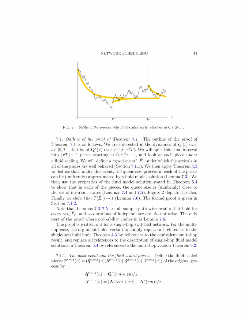
NETWORK SCHEDULING 41
Fig. 2. Splitting the process into fluid-scaled parts, starting at 0, r,2r, . . . .
7.1. Outline of the proof of Theorem 7.1. The outline of the proof ofTheorem 7.1 is as follows. We are interested in the dynamics of qr(t) overt ∈ [0, T ], that is, of Qr(τ) over τ ∈ [0, r2T ]. We will split this time intervalinto ⌊rT ⌋ + 1 pieces starting at 0, r,2r, . . . , and look at each piece under
a fluid scaling. We will define a “good event” Er under which the arrivals inall of the pieces are well behaved (Section 7.1.1). We then apply Theorem 4.3to deduce that, under this event, the queue size process in each of the piecescan be (uniformly) approximated by a fluid model solution (Lemma 7.3). Wethen use the properties of the fluid model solution stated in Theorem 5.4to show that in each of the pieces, the queue size is (uniformly) close tothe set of invariant states (Lemmas 7.4 and 7.5). Figure 2 depicts the idea.
Finally we show that P(Er)→ 1 (Lemma 7.6). The formal proof is given inSection 7.1.2.
Note that Lemmas 7.3–7.5 are all sample path-wise results that hold forevery ω ∈ Er, and so questions of independence etc. do not arise. The onlypart of the proof where probability comes in is Lemma 7.6.
The proof is written out for a single-hop switched network. For the multi-hop case, the argument holds verbatim; simply replace all references to thesingle-hop fluid limit Theorem 4.3 by references to the equivalent multi-hopresult, and replace all references to the description of single-hop fluid modelsolutions in Theorem 5.4 by references to the multi-hop version Theorem 6.2.
7.1.1. The good event and the fluid-scaled pieces. Define the fluid-scaledpieces xr,m,z(u) = (qr,m,z(u), ar,m,z(u), yr,m,z(u), sr,m,z(u)) of the original pro-cess by
qr,m,z(u) =Qr(rm+ zu)/z,
ar,m,z(u) = (Ar(rm+ zu)−Ar(rm))/z,
42 D. SHAH AND D. WISCHIK
yr,m,z(u) = (Yr(rm+ zu)−Yr(rm))/z,
sr,m,z(u) = (Sr(rm+ zu)− Sr(rm))/z
for 0≤m≤ ⌊rT ⌋, z ≥ r and u≥ 0. Here r indicates which process we are con-sidering, m indicates the piece and z indicates the fluid-scaling parameter.The scaling parameter zr,m = |Qr(rm)|∨ r is particularly important, and forconvenience we will define xr,m(u) = (qr,m(u), ar,m(u), yr,m(u), sr,m(u)) by
qr,m(u) = qr,m,zr,m(u), ar,m(u) = ar,m,zr,m(u),
yr,m(u) = yr,m,zr,m(u), sr,m(u) = sr,m,zr,m(u).
The good event is defined to be
Er ={
supu∈[0,Tfluid]
|ar,m,wr,k(u)−λru|< ηr for all 0≤m≤ ⌊rT ⌋(47)
and 0≤ k ≤ ⌊Lr log r⌋, where wr,k = r(1 + k/ log r)}
.
By this, we mean that Er is a subset of the sample space for the rth system,and we write xr,m,wr,k(·)(ω) etc. for ω ∈ Er when we wish to emphasize the
dependence on Er. The constants here are Tfluid = (2+λmax+NSmax)(Hζ +
1), λmax = supr |λr|, ζ > 0 is chosen as specified in Section 7.1.2 below,Hζ is chosen as in Theorem 5.4(v), L= 1 + T (1 + λmax +NSmax), Smax =maxπ∈S |π| and the sequence of deviation terms ηr ∈ [0,1] is chosen as spec-ified in Lemma 7.6 such that ηr → 0 as r→∞.
Lemma 7.3. Let FMS be the set of fluid model solutions over time hori-zon [0, T fluid] for arrival rate vector λ, and let FMS(q0) and FMS1 be asspecified in Definition 4.1. Then
supω∈Er
max0≤m≤⌊rT ⌋
d(xr,m(·)(ω),FMS1)→ 0 as r→∞(48)
and
supω∈Er
d(xr,0(·)(ω),FMS(q0))→ 0 as r→∞,(49)
where q0 = q0/(|q0| ∨ 1).
Proof. The proof of each equation will use Theorem 4.3. We startwith (48). The theorem requires the use of an index j in some totally or-dered countable set; here we shall use the pair j ≡ (r,m) ordered lexico-graphically, where r ∈ N and 0 ≤m≤ ⌊rT ⌋. Lexicographic ordering means(r,m)≥ (r′,m′) iff either r > r′ or both r = r′ and m≥m′. Note that j →∞implies r→∞ (and vice versa).
To apply the theorem, we first need to pick constants. Let K = 1, let λ
and λj = λr → λ as per Assumption 2.5 and let εj = ηr(1+ 1/ log r) so that
NETWORK SCHEDULING 43
εj → 0. Thus condition (23) of Theorem 4.3 is satisfied. Now let
Gj ≡Gr,m = {(xr,m(·)(ω), zr,m(ω)) :ω ∈ Er}.It is worth stressing that Gj ≡Gr,m is a set of sample paths and associatedscaling parameters, not a probabilistic event, and so any questions aboutthe lack of independence between xr,m(·)(ω) and zr,m(ω) are void. Note also
that although the events Er lie in different probability spaces for each r, thishas no bearing on the definition of Gj nor on the application of Theorem 4.3.
We next show that Gj satisfies conditions (24)–(26) of Theorem 4.3, for jsufficiently large. Equation (24) follows straightforwardly from the fact thatzr,m ≥ r, hence inf{z : (x, z) ∈ Gr,m} ≥ r, hence inf{z : (x, z) ∈ Gj} → ∞.
For (25), later in the proof we will establish that, under Er for r largeenough,
supt∈[0,Tfluid]
|ar,m(t)−λrt|< ηr
(
1 +1
log r
)
for all 0≤m≤ ⌊rT ⌋,(50)
which implies that for all (x, z) ∈ Gj ≡Gr,m, supt∈[0,Tfluid]|aj(t)− λjt|< εjas required. Equation (26) follows straightforwardly from the scaling used
to define qj(0)≡ qr,m(0): for every ω, not merely ω ∈ Er,
|qr,m(0)|=∣
∣
∣
∣
Qr(rm)
zr,m
∣
∣
∣
∣
=
∣
∣
∣
∣
Qr(rm)
|Qr(rm)| ∨ r
∣
∣
∣
∣
≤ 1.
Since Gj satisfies the conditions of Theorem 4.3 for sufficiently large j,we can apply that theorem to deduce
sup(x,z)∈Gj
d(x,FMS1)→ 0 as j →∞.
Rewriting j as (r,m), and turning the limit statement into a limsup state-ment,
sup(r′,m)≥(r,0)
sup(x,z)∈Gr′,m
d(x,FMS1)→ 0 as r→∞
and in particular
max0≤m≤⌊rT ⌋
sup(x,z)∈Gr,m
d(x,FMS1)→ 0 as r→∞.
Rewriting (x, z) ∈Gr,m in terms of ω ∈ Er, as per the definition of Gr,m,
max0≤m≤⌊rT ⌋
supω∈Er
d(xr,m(·)(ω),FMS1)→ 0 as r→∞.
Interchanging the max and the sup gives (48).To establish (49), we will again apply Theorem 4.3 but this time using
the index j ≡ r, λj = λr →λ and εj = ηr(1 + 1/ log r) as above, and define
Gj ≡Gr = {(xr,0(·)(ω), zr,0(ω)) :ω ∈ Er}.
44 D. SHAH AND D. WISCHIK
Equations (23)–(26) hold just as before. For (28), we will use q0 as in thestatement of this lemma, and ε′j = |qr,0(0)− q0|. This is a well-defined con-stant (i.e., it does not depend on the randomness ω), because we assumedin Theorem 7.1 that the initial queue sizes Qr(0) are nonrandom, and bydefinition qr,0(0) =Qr(0)/(|Qr(0)| ∨ r). Furthermore, Theorem 7.1 assumes
qr(0) → q0, which implies qr,0(0) → q0 hence ε′j → 0. Equation (28) then
follows straightforwardly, for every ω not merely ω ∈ Er. Applying Theo-rem 4.3, we deduce that
sup(x,z)∈Gj
d(x,FMS(q0))→ 0 as j →∞.
Equivalently,
supω∈Er
d(xr,0(·)(ω),FMS(q0))→ 0 as r→∞
as required.To complete the proof of Lemma 7.3, the only remaining claim that needs
to be established is (50). We will proceed in two steps. First we prove that
|Qr(rm)| ≤ Lr2 under Er, for r sufficiently large and for all 0≤m≤ ⌊rT ⌋.To see this, note from (7) that
Qr(rm)≤Qr(0) +Ar(rm) +NrmSmax.
Now Er gives a suitable bound on arrivals: for all 0≤m′ ≤ ⌊rT ⌋, and usingthe fact that 1≤ T fluid,
∣
∣
∣
∣
Ar(rm′ + r)−Ar(rm′)
r− λr
∣
∣
∣
∣
= |ar,m′,wr,0(1)−λr|< ηr,
and by applying this fromm′ = 0 tom′ =m−1 we find |Ar(rm)| ≤ rm(λmax+ηr). The assumptions of Theorem 7.1 tell us that Qr(0)/r → q0 for someq0 ∈R
N+ . Putting all this together, we find that for sufficiently large r
|Qr(rm)| ≤ r2(1 + T (1 + λmax +NSmax)) = Lr2 for any 0≤m≤ ⌊rT ⌋.
Now we proceed to prove (50), under Er for r sufficiently large. Observe that(for r > 2) there exists k ∈ {1, . . . , ⌊Lr log r⌋} such that wr,k−1 ≤ zr,m ≤wr,k;this follows from r ≤ zr,m = |Qr(rm)| ∨ r ≤ Lr2 and the definition of wr,k
in (47). Hence for any t ∈ [0, T fluid],
|ar,m(t)−λrt|
=
∣
∣
∣
∣
Ar(rm+ zr,mt)−Ar(rm)
zr,m−λrt
∣
∣
∣
∣
=
∣
∣
∣
∣
Ar(rm+wr,ku)−Ar(rm)
wr,k−λru
∣
∣
∣
∣
(
wr,k
zr,m
)
where u= tzr,m/wr,k
NETWORK SCHEDULING 45
= |ar,m,wr,k(u)−λru|(
wr,k
zr,m
)
< ηrwr,k
zr,msince Er holds and u≤ t≤ T fluid
≤ ηrwr,k
wr,k−1since zr,m ≥wr,k−1
= ηr
(
1 +1
k− 1 + log r
)
≤ ηr
(
1 +1
log r
)
.
This establishes (50) and completes the proof. �
Lemma 7.4 (Choice of approximating piece). Given t ∈ [0, T ] and r ∈N,define m∗ =m∗(r, t) and u∗ = u∗(r, t) by
m∗ =min{m ∈ Z+ : rm≤ r2t≤ rm+ T fluidzr,m}, u∗ =r2t− rm∗
zr,m∗.
This is a sound definition (i.e., the set for m∗ is nonempty). Further, under
event Er, either m∗ = 0 and 0 ≤ u∗ ≤ T fluid, or 0 < m∗ ≤ ⌊rT ⌋ and Hζ <u∗ ≤ T fluid.
Proof. The set for m∗ is nonempty because zr,m ≥ r and T fluid ≥ 1. Theupper bound form∗ is trivial. The upper bound for u∗ in either case is trivial.To prove the lower bound for u∗ whenm∗ > 0, r2t > r(m∗−1)+T fluidzr,m∗−1
due to the minimality of m∗. Hence
u∗ =r2t− rm∗
zr,m∗>
T fluidzr,m∗−1 − r
zr,m∗≥ T fluid zr,m∗−1
zr,m∗− 1.
To bound zr,m∗−1/zr,m∗ , we can use (7) and the bound on ar,m,wr,0(1) pro-
vided by Er to show that for any m
zr,m = |Qr(rm)| ∨ r
≤ (|Qr(rm− r)|+ r(λmax + ηr +NSmax)) ∨ r
≤ |Qr(rm− r)| ∨ r+ r(λmax +1+NSmax) since ηr ≤ 1
≤ zr,m−1(2 + λmax +NSmax) since zr,m−1 ≥ r.
Substituting this back into the earlier bound for u∗,
u∗ >T fluid
2 + λmax +NSmax− 1,
and this is equal to Hζ by choice of T fluid. �
Lemma 7.5 (Pathwise multiplicative state space collapse). Let 0< ζ < 1,t ∈ [0, T ] and r ∈ N be given. Suppose there exist m ∈ {0, . . . , ⌊rT ⌋}, u ∈[0, T fluid] and x ∈ FMS such that r2t= rm+ zr,mu and ‖xr,m − x‖< ζ, andfurthermore either (i) m> 0 and u >Hζ and x ∈ FMS1, or (ii) m= 0 and
46 D. SHAH AND D. WISCHIK
x ∈ FMS(q0) where q0 is as defined in Lemma 7.3. Then
|qr(t)−∆W (qr(t))|‖qr(·)‖ ∨ 1
≤ |qr(t)−∆W (qr(t))|zr,m/r
< 2ζ +mcζ(∆W ),(51)
where mcζ(∆W ) is the modulus of continuity of the map q 7→∆W (q) over
D= {q′ ∈RN+ : |q′ − q| ≤ 1 for some q such that L(q)≤L(1)}
for L(·) as in Definition 5.3.
Proof. The first inequality is trivially true because
zr,mr
=|Qr(rm)| ∨ r
r≤(
supu∈[0,T ]
qr(u))
∨ 1.
For the second inequality, note that after unwrapping the qr(·) scaling andwrapping it up again in the qr,m scaling, the middle term in (51) is
MT= |qr,m(u)−∆W (qr,m(u))|.Writing q for the queue component of x,
MT≤ |qr,m(u)− q(u)|+ |q(u)−∆W (q(u))|+ |∆W (q(u))−∆W (qr,m(u))|= (52a) + (52b) + (52c) respectively.
We can bound each term as follows:
is < ζ since ‖xr,m − x‖< ζ by an assumption of the lemma.(52a)
(52b) is < ζ in the case m > 0: by the assumptions of the lemma,x ∈ FMS1 so |q(0)| ≤ 1, and also u >Hζ . The requirements of The-orem 5.4(v) are met; hence we obtain the inequality.
is = 0 in the case m∗ = 0: In this case, by assumption of the lemmax ∈ FMS(q0), that is, q(0) = q0. By assumption of Theorem 7.1q0 ∈ I, that is, q0 =∆W (q0), therefore by Theorem 5.4(iii) q0 ∈ I,therefore by Theorem 5.4(iv) the fluid model solution q(·) staysconstant at q0 and so (52b) = 0.
(52c) is ≤ mcζ(∆W ): by assumption of the lemma, either m > 0 andx ∈ FMS1, or m = 0 and x ∈ FMS(q0) where q0 ≤ 1 component-wise; either way q(0) ≤ 1 componentwise, so L(q(0)) ≤ L(1). ByTheorem 5.4(i) L(q(u)) ≤ L(1) so q(u) ∈ D. Furthermore, since‖xr,m−x‖< ζ by assumption of the lemma, |qr,m(u)−q(u)|< ζ < 1and so qr,m(u) ∈D. The inequality then follows from the definitionof the modulus of continuity. �
Lemma 7.6 (The good event has high probability). Under the assump-
tions of Theorem 7.1, P(Er)→ 1 as r →∞. The deviation terms are givenby ηr =min(1, supz≥r T
fluidδ⌊zTfluid⌋) and ηr → 0 as r→∞.
NETWORK SCHEDULING 47
Proof. By a simple union bound, and then using the fact that thearrival process has stationary increments,
P(Er)≥ 1−⌊rT ⌋∑
m=0
⌊Lr log r⌋∑
k=0
P
(
supu∈[0,Tfluid]
|ar,m,wr,k(u)− λru| ≥ ηr
)
= 1− (1 + ⌊rT ⌋)⌊Lr log r⌋∑
k=0
P
(
supu∈[0,Tfluid]
|ar,0,wr,k(u)−λru| ≥ ηr
)
= 1− (1 + rT )
⌊Lr log r⌋∑
k=0
P
(
supu∈[0,Tfluid]
∣
∣
∣
∣
Ar(wr,ku)
wr,k−λru
∣
∣
∣
∣
≥ ηr
)
.
To bound this we will use Assumption 2.5, which says that
z(log z)2P
(
supτ≤z
1
z|Ar(τ)−λrτ | ≥ δz
)
→ 0 as z→∞
uniformly in r. After extending the domain of Ar to R+ by linear interpo-lation in each interval (τ, τ + 1), and extending the domain of δz to z ∈R+
by δ(z) = δ⌊z⌋ ∨ δ⌈z⌉, and rescaling z by T fluid,
z(log z)2P
(
supu∈[0,Tfluid]
∣
∣
∣
∣
Ar(zu)
z−λru
∣
∣
∣
∣
≥ T fluidδ(zT fluid)
)
→ 0 as z→∞
uniformly in r. In other words, for any φ > 0 there exists z0 such that forall z ≥ z0 and all r,
P
(
supu∈[0,Tfluid]
∣
∣
∣
∣
Ar(zu)
z−λru
∣
∣
∣
∣
≥ T fluidδ(zT fluid)
)
<φ
z(log z)2.
Now pick r0 sufficiently large that r0 ≥ z0 and supz≥r0 Tfluidδ(zT fluid) < 1,
which we can do since δ(z) → 0 as z →∞ by Assumption 2.5. This choiceimplies that for any r ≥ r0 and z ≥ r, T fluidδ(zT fluid)≤ ηr [recall that ηr =min(1, supz≥r T
fluidδ⌊zTfluid⌋)]. Hence, for any r≥ r0 and z ≥ r,
P
(
supu∈[0,Tfluid]
∣
∣
∣
∣
Ar(zu)
z−λru
∣
∣
∣
∣
≥ ηr
)
<φ
z(log z)2.
Applying this bound to P(Er), and using the facts that wr,k ≥ r andwr,k(logwr,k)
2 ≥ r(1 + k/ log r)(log r)2,
1− P(Er)< φ
(
1 + ⌊rT ⌋r(log r)2
) ⌊Lr log r⌋∑
k=0
1
1 + k/ log r
= φ
(
1 + ⌊rT ⌋r log r
) ⌊Lr log r⌋∑
k=0
1
k+ log r
48 D. SHAH AND D. WISCHIK
≤ φ
(
1 + ⌊rT ⌋r log r
)∫ ⌊Lr log r⌋
ℓ=0
1
ℓ− 1 + log rdℓ
= φ
(
1 + ⌊rT ⌋r log r
)
log
(
1 +⌊Lr log r⌋log r− 1
)
.
The final expression converges to φT as r → ∞. Since φ can be chosenarbitrarily small, P(Er)→ 1 as r→∞. �
7.1.2. Proof of Theorem 7.1. Given δ > 0, pick ζ > 0 such that 2ζ +mcζ(∆W ) < δ ∧ 1 where mcζ(∆W ) is the modulus of continuity of ∆Wover the set D specified in Lemma 7.5. We can achieve the desired boundby making ζ sufficiently small; this is because ∆W is continuous, henceuniformly continuous on compact sets, and D is compact as a consequenceof Theorem 5.4(i), hence mcζ(∆W ) → 0 as ζ → 0. With this choice of ζ ,
define the good sets Er and the constants T fluid and Hζ as specified by (47).
By Lemma 7.3, there exists r0 such that for r ≥ r0 and for all ω ∈ Er andall m, d(xr,m,FMS1) < ζ and d(xr,0,FMS(q0)) < ζ , where q0 is defined inthe statement of the lemma.
Now, pick any t ∈ [0, T fluid] and r≥ r0, and assume Er holds. Lemma 7.4says that we can choose m ∈ {0, . . . , ⌊rT ⌋} and u ∈ [0, T fluid] such that r2t=rm+ zr,mu, and furthermore either (i) m> 0 and u >Hζ or (ii) m= 0. ByLemma 7.3, we can pick x ∈ FMS (depending on r, t and the ω) such that‖xr,m−x‖< ζ and furthermore either (i) m> 0 and x ∈ FMS1 or (ii) m= 0and x ∈ FMS(q0). Then, by Lemma 7.5,
|qr(t)−∆W (qr(t))|‖qr(·)‖ ∨ 1
< δ.
This bound holds for every t ∈ [0, T ] and r≥ r0, in a sample path-wise sense,
whenever ω ∈ Er.Finally, Lemma 7.6 says that P(Er)→ 1. This completes the proof. �
8. An optimal policy? Our motivation for this work was Conjecture 3.1,which says that for an input-queued switch the performance of MW-α im-proves as α ց 0. We have not been able to prove this. However, undera condition on the arrival rate, we can show (i) that the critically-loadedfluid model solutions for a single-hop switched network approach optimal(in the sense of minimizing total amount of work in the network) as αց 0;and (ii) that for an input-queued switch the set of invariant states I de-fined in Section 7 is sensitive to α. We speculate that these findings mighteventually form part of a proof of a heavy traffic limit theorem supportingConjecture 3.1, given that critically loaded fluid models and invariant statesplay an important role in heavy traffic theorems.
NETWORK SCHEDULING 49
In this section we state the condition on the arrival rates, and give theresults (i) and (ii). Motivated by these results, we make a conjecture aboutan optimal scheduling policy.
Definition 8.1 (Complete loading). Consider a switched network witharrival rate vector λ. Say that λ satisfies the complete loading condition ifλ ∈ Λ, and there is a convex combination of critically loaded virtual resourcesthat gives equal weight to each queue; in other words if
1
maxπ∈S 1 ·π ∈ 〈Ξ(λ)〉.
Theorem 8.2 (Near-optimality of fluid models under complete loading).Consider a single-hop switched network with arrival rate vector λ ∈Λ.
(i) For any fluid model solution for the MW-α policy, 1 · q(t) ≤Nα/(1+α)1 · q(0).
(ii) For any fluid model solution for any scheduling policy, if λ satisfiesthe complete loading condition, then 1 · q(t)≥ 1 · q(0).
Proof. The first claim relies on the standard result that for any x ∈RN+
and β > 1,
1
N1−1/β
∑
n
xn ≤(
∑
n
xβn
)1/β
≤∑
n
xn.(53)
Using the Lyapunov function from Definition 5.3,
1 · q(t)≤N1−1/(1+α)
(
∑
n
qn(t)1+α
)1/(1+α)
by the first inequality in (53)
=Nα/(1+α)L(q(t))1/(1+α) by definition of L(·)≤Nα/(1+α)L(q(0))1/(1+α) since L(q(t))≤ 0 by Theorem 5.4(i)
≤Nα/(1+α)1 · q(0) by the second inequality in (53).
The second claim is a simple consequence of Lemma 5.10. (This lemma isfor a single-hop network. The multi-hop version, Lemma 6.8, does not havesuch a simple interpretation.) �
Theorem 8.3 (I is sensitive to α for an input-queued switch). Consideran M×M input-queued switch running MW-α, as introduced in Section 2.4.Let λij be the arrival rate at the queue at input port i of packets destined for
output port j, λ ∈RM×M+ . Suppose that λ> 0 componentwise, and further-
more that every input port and every output port is critically loaded, that
50 D. SHAH AND D. WISCHIK
is,
M∑
j=1
λıj = 1 and
M∑
i=1
λi = 1 for every 1≤ ı, ≤M.(54)
Then λ satisfies the complete loading condition, and the critically loadedvirtual resources are
Ξ(λ) = {rı for all 1≤ ı≤M} ∪ {c for all 1≤ ≤M},where rı and c are the row and column indicator matrices, (rı)i,j = 1i=ı
and (c)i,j = 1j=. Define the workload map W :RM×M+ → R
2M+ by W (q) =
[ξ · q]ξ∈Ξ(λ). Denoting the invariant set by I(α):
(i) if w is in the relative interior of {W (q) :q ∈ RM×M+ }, then w is in
{W (q) :q ∈ I(α)} for sufficiently small α> 0;(ii) for a 2×2 input-queued switch, {W (q) :q ∈ I(α)} is strictly increas-
ing as αց 0.
Item (i) essentially says that W (I(α)) becomes as large as possible asαց 0, except for some possible issues at the boundary. We have only beenable to prove (ii) for a 2× 2 switch, but we believe it holds for any M ×Mswitch. The proofs are rather long, and depend on the specific structure ofthe input-queued switch, so they are left to the Appendix.
Conjecture 3.1 claims that, for an input-queued switch, performance im-proves as αց 0. Examples due to Ji, Athanasopoulou and Srikant [15] andStolyar (personal communication) show that this is not true for generalswitched networks. However, Theorem 8.2 suggests that the conjecture mightapply not just to input-queued switches but also to generalized switches un-der the complete loading condition; the examples of Ji, Athanasopoulou andSrikant [15] and Stolyar do not satisfy this condition. We therefore extendConjecture 3.1 as follows.
Conjecture 8.4. Consider a general single-hop switched network asdescribed in Section 2, running MW-α. Consider the diffusion scaling limit(described in Conjecture 7.2), and let λ be the limiting arrival rates; as-sume λ satisfies the complete loading condition. For every α > 0 there isa limiting stationary queue size distribution. The expected value of the sumof queue sizes under this distribution is nonincreasing as αց 0.
Theorem 8.2 says that MW-α approaches optimal as α ց 0, under thecomplete loading condition. It is natural to ask if there is a policy that isoptimal, rather than just a sequence of policies that approach optimal. Giventhat MW-α chooses a schedule π to maximize π · qα (where the exponent
NETWORK SCHEDULING 51
is taken componentwise), and since
xα =
{
1 +α logx+O(α2), if x > 0,0, if x= 0,
we propose the following formal limit policy, which we call MSMW-log: ateach time step, look at all maximum-size schedules, that is, those π ∈ S forwhich
∑
n πn1Qn>0 is maximal. Among these, pick one which has maximallog-weight, that is, for which
∑
n :Qn>0 πn logQn is maximal, breaking tiesrandomly.
Conjecture 8.5. Consider a general single-hop switched network run-ning MSMW-log. Consider the diffusion scaling limit, and let λ be the lim-iting arrival rates; assume λ satisfies the complete loading condition. Thereis a limiting stationary queue size distribution. This distribution minimizesthe expected value of the sum of the queue sizes, over all scheduling policiesfor which this expected value is defined.
Scheduling policies based on MW are computationally difficult to imple-ment because there are so many comparisons to be made. In future workwe plan to investigate whether the techniques described in this paper canbe applied to policies that may have worse performance but simpler imple-mentation.
APPENDIX: RESULTS FOR INPUT-QUEUED SWITCHES
In this section we prove Theorem 8.3. Throughout this Appendix we areconsidering a M ×M input-queued switch. The set of schedules S consistsof all M ×M permutation matrices. We assume the arrival rate matrix λsatisfies the complete loading condition (54) and that λ> 0 componentwise.We let the scheduling algorithm be MW-α, and define I(α) to be the set ofinvariant states.
A.1. Identifying Λ, S∗, Ξ and Ξ+. The Birkhoff–von Neumann decom-position result says that a matrix is doubly substochastic if and only if it isless than or equal to a convex combination of permutation matrices, whichyields
Λ =
{
λ∈ [0,1]M×M :
M∑
j=1
λı,j ≤ 1 and
M∑
i=1
λi, ≤ 1 for all ı,
}
.
Since λ satisfies the complete loading condition (54), λ ∈ Λ.Lemma A.1 below gives S∗, the set of virtual resources, that is, maximal
extreme points of the set of feasible solutions to DUAL(λ). From the com-plete loading condition, it is clear that Ξ(λ) = S∗ as claimed in the theorem.It will also be useful, for the proof of Theorem 8.3(i), to identify Ξ+(λ) as
52 D. SHAH AND D. WISCHIK
defined by (34). We claim that
Ξ+(λ) = Ξ(λ).(55)
To see this, suppose ξ is a nonmaximal extreme point of the set of feasiblesolutions to DUAL(λ); then there exists some other extreme point ζ suchthat ξ ≤ ζ and ξ 6= ζ; but because λ > 0 componentwise it must be thatξ ·λ< ζ ·λ. We have found that λ ∈ Λ, so the solution to DUAL(λ) is ≤ 1,hence ξ ·λ< 1. Therefore ξ /∈ Ξ+(λ), that is, Ξ+(λ) consists only of maximalextreme points.
Lemma A.1. The set of maximal extreme points of the set
F = {ξ ∈RM×M+ :ξ ·π ≤ 1 for all π ∈ S}
is given by
S∗ = {rı for all 1≤ ı≤M} ∪ {c for all 1≤ ≤M},where the row and column indicator matrices rı and c are defined by (rı)i,j =1i=ı and (c)i,j = 1j=.
Proof. First we argue that every ξ ∈ S∗ is a maximal extreme pointof F . It is simple to check that ξ ∈ F . Also, ξ is extreme because F ⊂[0,1]M×M . Finally, ξ is maximal because if it were not then there wouldbe some ε ≥ 0, ε 6= 0, such that ξ + ε ∈ F ; but for any such ε there isa matching π such that ε ·π > 0 hence ξ+ ε /∈ F .
Next we argue the converse, that all maximal extreme points of F arein S∗. The first step is to characterize the extreme points of F . We claimthat if ζ ∈ F , then it can be written ζ ≤ ξ for some ξ ∈ 〈S∗〉. Consider theoptimization problem
minimizeM∑
ı=1
xı +M∑
=1
y over xı ≥ 0, y ≥ 0 for all ı,
(56)such that ζ ≤
∑
ı
xırı +∑
yc.
The dual of this problem is
maximize a · ζ over a ∈RM×M+
(57)such that a · rı ≤ 1, a · c ≤ 1 for all ı, .
[These problems are just PRIMAL(ζ) and DUAL(ζ), resp., but with respectto the “virtual” schedule set S∗ rather than the actual schedule set S .] BySlater’s condition, strong duality holds. Now, any matrix a that is feasiblefor (57) is nonnegative and doubly substochastic, hence by the Birkhoff–von Neumann decomposition result it can be written as a a ≤ b where b
is a convex combination of permutation matrices, that is, b ∈ 〈S〉. But bythe assumption that ζ ∈ F , ζ · π ≤ 1 for all π ∈ S , hence b · ζ ≤ 1, hence
NETWORK SCHEDULING 53
a · ζ ≤ 1, so the value of the optimization problem (57) is ≤ 1. By strongduality, the value of the optimization problem (56) is also ≤ 1. Thereforeζ ≤ ξ for some ξ ∈ 〈S〉.
We now claim that if ζ ∈ F then it can be written ζ =∑
ξ aξξ where thesum is over some finite collection of values drawn from the set
E = {ξ ∈RM×M+ :ξ ≤ rı or ξ≤ c for some ı, },
and all aξ are ≥ 0. We have just shown that
ζ =∑
ξ
aξξ− z for some z≥ 0 and aξ ≥ 0, ξ ∈E.(58)
If z = 0 we are done. Otherwise, pick some (k, l) such that zk,l > 0 anddefine nk,l by (nk,l)i,j = 1− 1i=k and j=l. Noting that
∑
aξξk,l ≥ zk,l > 0, wecan rewrite ζ as
ζ =zk,l
∑
aξξk,l
∑
aξξ+
(
1− zk,l∑
aξξk,l
)
∑
aξξnk,l − znk,l,
where matrix multiplication is componentwise as per the notation specifiedin Section 1. We have thus rewritten ζ in the form (58), but now z has onefewer nonzero element. Continuing in this way we can remove all nonzeroelements of z, until we are left with ζ ∈ 〈E〉.
We have therefore shown that all extreme points of F are in E. Clearly,all maximal points of E are in S∗. Therefore, all the maximal extreme pointsof F are in S∗ as claimed. �
A.2. Proof of Theorem 8.3(i). We first state two lemmas which will beneeded in the proof. The first is a general closure property of permutationmatrices, and the second is a property of invariant states of MW-α. We thenprove the theorem and the two lemmas.
Lemma A.2. Let x ∈ RM×M+ , and define A ∈ R
M×M+ by Ai,j = 1 if
there is some matching ρ ∈ S whose weight ρ · x is maximal (i.e., ρ · x =maxσ∈S σ · x) and for which ρi,j = 1; and Ai,j = 0 otherwise. Then, for anymatching π such that
πi,j = 1 =⇒ Ai,j = 1,
π is itself a maximum weight matching.
Lemma A.3. Fix any λ ∈ Λ, and any q ∈ I(α). For every 1≤ i, j ≤Msuch that λi,j > 0, there exists a matching π ∈ S whose weight π · qα ismaximal (i.e., π · qα =maxσ∈S σ · qα, where the exponent is taken compo-nentwise) and for which πi,j = 1.
Proof of Theorem 8.3(i). Suppose the claim of the theorem is nottrue, that is, that there exists a sequence α ց 0 such that w /∈ W(α) ={W (q) :q ∈ I(α)} for each α in the sequence.
54 D. SHAH AND D. WISCHIK
Write w = (w1·, . . . ,wM ·,w·1, . . . ,w·M), and define the function ∆α :R2M+ →
RM×M+ to give the (unique) solution to the optimization problem
minimize1
1 + α
∑
i,j
q1+αi,j over q ∈R
M×M+
such that rı · q≥wı· and c · q≥w· for all 1≤ ı, ≤M.
This is the optimization problem defined in (35); we have simply writtenout Ξ+(λ) explicitly using (55). By Lemma 5.6, the map ∆W :RM×M
+ →RM×M+ that defines I(α) is simply the composition of W :RM×M
+ → R2M+
and ∆α :R2M+ → R
M×M+ . Let q(α) = ∆α(w). Note that q(α) ∈ I(α); this is
because q(α) is optimal for ∆α(w), therefore it is optimal for ∆α(W (q(α)))which has a smaller feasible region, therefore q(α) = ∆α(W (q(α))) =∆W (q(α)), that is, q(α) ∈ I(α).
We next establish this claim: that for each α in the sequence, there exists i,j, i′ and j′ such that qi,j(α) = 0, qi′,j(α) ≥ w·j/M and qi,j′(α) ≥ wi·/M .To prove this claim, observe that W (q(α)) ≥ w by the constraints of theoptimization problem ∆α; and that q(α) ∈ I(α) hence W (q(α)) ∈ W(α);hence W (q(α)) 6=w by assumption that w /∈W(α). Therefore W (q(α))>win some component, that is, there is some i or j such that ri ·q(α)>wi· or cj ·q(α)>w·j . Indeed, there must be both such an i and j, since otherwise thesum of row workloads and column workloads would not be equal. Thereforeqi,j(α) = 0, since if qi,j(α) > 0, then we could reduce qi,j(α) and still havea feasible solution to the problem that defines ∆α(w) but with a smallervalue of the objective function, which contradicts optimality of q(α). Theremust also be a j′ such that qi,j′(α) ≥ wi·/M since otherwise the workloadconstraint ri · q(α)≥wi· would not be met. Likewise for i′.
We assumed that w ∈R2M+ is in the relative interior ofWmax = {W (q) :q ∈
RM×M+ }. This set is clearly convex, and from the characterization of relative
interior for convex sets, for all x ∈Wmax there exists y ∈Wmax and 0< a< 1such that w = ax+ (1− a)y. In particular, by choosing x=W (1), we findthat w > 0 componentwise.
For each α in the sequence we can find indices (i(α), j(α), i′(α), j′(α)) asabove. Some set of indices (i, j, i′, j′) must be repeated infinitely often, sincethere are only finitely many choices. Restrict attention to the subsequenceof α for which i(α) = i, j(α) = j, i′(α) = i′, j′(α) = j′.
Now, consider the submatrix(
qi,j(α) qi,j′(α)qi′,j(α) qi′,j′(α)
)
.
Recall that q(α) ∈ I(α). By Lemma A.3, and the assumption that λ > 0
componentwise, every queue is involved in some maximum weight matching.By Lemma A.2, every matching is a maximum weight matching. Let π beany matching with πi,j = πi′,j′ = 1, and let ρ be like π except with (i, j) and
NETWORK SCHEDULING 55
(i′, j′) flipped, that is, ρi,j = ρi′,j′ = 0 and ρi,j′ = ρi′,j = 1. We can write outexplicitly the difference in weight between these two matchings
ρ · q(α)α −π · q(α)α = qi′,j(α)α + qi,j′(α)
α − qi′,j′(α)α − qi,j(α)
α.
Here, q(α)α denotes component-wise exponentiation. Recall that along thesubsequence we have chosen, qi,j(α) = 0, qi,j′(α) ≥ wi·/M and qi′,j(α) ≥w·j/M . Therefore lim infα→0 ρ · q(α)α −π · q(α)α > 0. This contradicts thefinding that every matching is a maximum weight matching for q(α).
Thus, we have contradicted our original assumption that there exists a se-quence αց 0 with w /∈W(α). This completes the proof. �
Proof of Lemma A.2. Let a=maxρ ρ · x be the weight of the max-imum weight matching, let A = {ρ :ρ · x = a} and let σ =
∑
ρ∈Aρ. Ob-
serve that σ ∈ ZM×M+ and Ai,j = 1{σi,j>0}. Therefore, σ ≥A componentwise.
Further, by definition A≥ π. Therefore, the matrix σ − π is nonnegative.Since σ is sum of |A| permutation matrices, all its row sums and columnsums are equal to |A|. And since π is a permutation matrix as well, the ma-trix σ−π has all its row sums and column sums equal to |A|− 1; thereforeby the Birkhoff–von Neumann decomposition
σ =π+∑
ρ∈S
αρρ,
where each αρ ≥ 0 and∑
αρ = |A| − 1. Now, σ · x= |A|a by constructionof σ. Therefore
|A|a= σ · x= π · x+∑
ρ∈S
αρρ · x
≤ π · x+ (|A| − 1)a because a=maxρ∈S
ρ · x.
Rearranging, π ·x≥ a. But a is the weight of the maximum weight matching,thus π · x= a. �
Proof of Lemma A.3. Since λ ∈ Λ, λ≤ σ for some σ ∈ 〈S〉, that is,σ =
∑
π∈S aππ where∑
aπ = 1 and each aπ ≥ 0. Therefore
λ · qα ≤ σ · qα =∑
aππ · qα ≤(
∑
aπ
)
maxπ∈S
π · qα =maxπ∈S
π · qα.
But by Lemma 5.11(iv), λ ·qα =maxππ ·qα, therefore both the inequalitiesin the above must be equalities. In particular, all matchings π for whichaπ > 0 are maximum weight matchings. If λi,j > 0, then at least one of thesematchings has πi,j = 1. �
A.3. Proof of Theorem 8.3(ii). Consider a 2× 2 switch with arrival ratematrix λ. Since λ satisfies (54), we may write
λ=
(
λ1,1 1− λ1,1
1− λ1,1 λ1,1
)
56 D. SHAH AND D. WISCHIK
for some λ1,1 ∈ (0,1). To find I(α) we use the characterization from Lem-ma 5.11(iv), which says that q ∈ I(α) if and only if λ · qα = maxππ · qα,that is, if and only if
λ1,1(qα1,1 + qα2,2) + (1− λ1,1)(q
α1,2 + qα2,1) = (qα1,1 + qα2,2)∨ (qα1,2 + qα2,1).
Now, the equation λ1,1x+(1−λ1,1)y = x∨ y is satisfied if and only if x= y,given 0< λ1,1 < 1. Therefore
I(α) = {q ∈R2×2+ : qα1,1 + qα2,2 = qα1,2 + qα2,1}.
We wish show that {W (q) :q ∈ I(α)} is strictly increasing as αց 0, where
W (q) = (r1 ·q,r2 ·q,c1 ·q,c2 ·q). It suffices to show that W(α) = {W (q) :q ∈I(α)} is strictly increasing, where W (q) = (r1 · q,c1 · q,1 · q), since there is
a straightforward bijection between W (q) and W (q). Now, (w1·,w·1,w··) ∈R3+ is in W(α) iff there exists q ∈R
2×2+ such that
qα1,1 + qα2,2 = qα1,2 + qα2,1, r1 · q=w1·, c1 · q=w·1, 1 · q=w··,
that is, iff there exists x ∈R such that
xα + (w·· −w1· −w·1 + x)α − (w1· − x)α − (w·1 − x)α = 0,(59)
max(0,w1· +w·1 −w··)≤ x≤min(w1·,w·1).(60)
Write θ(x) for the left-hand side of (59). Since θ(x) is increasing in x, thereexists a solution to (59) iff θ(x)≤ 0 at the lower bound in (60) and θ(x)≥ 0at the upper bound. By considering four separate cases of which of thebounds in (60) are tight, and after some algebra, we find that there existsa solution iff
wi· +w·j + (wαi· +wα
·j)1/α ≥w·· for each i, j ∈ {1,2},(61)
where w2· = w·· −w1· and w·2 = w·· −w·1. Now, it is a standard inequalitythat for any x > 0 and y > 0, and any 0<α< β,
(xα + yα)1/α > (xβ + yβ)1/β .
Applying this inequality to (61), it follows that W(α) is strictly increasingas αց 0.
Acknowledgments. We would like to thank Mike Harrison, Frank Kelly,Balaji Prabhakar and Ruth Williams for helpful discussions. We thank Cia-mac Moallemi for suggesting Lemma 5.8. We also thank the anonymousreviewers for their help in improving readability of the manuscript.
REFERENCES
[1] Andrews, M., Kumaran, K., Ramanan, K., Stolyar, S., Vijayakumar, R. andWhiting, P. (2004). Scheduling in a queueing system with asynchronously vary-ing service rates. Probab. Engrg. Inform. Sci. 18 191–217. MR2037364
[2] Azuma, K. (1967). Weighted sums of certain dependent random variables. TohokuMath. J. (2) 19 357–367. MR0221571
NETWORK SCHEDULING 57
[3] Bramson, M. (1998). State space collapse with application to heavy traffic limits formulticlass queueing networks. Queueing Syst. 30 89–148. MR1663763
[4] Bramson, M. (2008). Stability of Queueing Networks. Lecture Notes in Math. 1950.Springer, Berlin. MR2445100
[5] Dai, J. G. (1999). Stability of fluid and stochastic processing networks. MaPhyStoLecture Notes. Available at http://www.maphysto.dk/cgi-bin/gp.cgi?
publ=70.[6] Dai, J. G. and Lin, W. (2005). Maximum pressure policies in stochastic processing
networks. Oper. Res. 53 197–218. MR2131925[7] Dai, J. G. and Lin, W. (2008). Asymptotic optimality of maximum pressure policies
in stochastic processing networks. Ann. Appl. Probab. 18 2239–2299. MR2473656[8] Dai, J. G. and Prabhakar, B. (2000). The throughput of switches with and without
speed-up. In Proceedings of IEEE Infocom 556–564. Tel-Aviv, Israel.[9] Dembo, A. and Zeitouni, O. (1998). Large Deviations Techniques and Applica-
tions, 2nd ed. Stochastic Modelling and Applied Probability 38. Springer, Berlin.MR2571413
[10] Doob, J. L. (1953). Stochastic Processes. Wiley, New York. MR1038526[11] Harrison, J. M. (1995). Balanced fluid models of multiclass queueing networks:
A heavy traffic conjecture. In Stochastic Networks. The IMA Volumes in Math-ematics and its Applications 71 1–20. Springer, New York. MR1381003
[12] Harrison, J. M. (2000). Brownian models of open processing networks: Canonicalrepresentation of workload. Ann. Appl. Probab. 10 75–103. MR1765204
[13] Harrison, J. M. (2003). Correction: “Brownian models of open processing networks:Canonical representation of workload” [Ann. Appl. Probab. 10 (2000) 75–103;MR1765204 (2001g:60230)]. Ann. Appl. Probab. 13 390–393. MR1952004
[14] Hoeffding, W. (1963). Probability inequalities for sums of bounded random vari-ables. J. Amer. Statist. Assoc. 58 13–30. MR0144363
[15] Ji, T., Athanasopoulou, E. and Srikant, R. (2009). Optimal scheduling policiesin small generalized switches. In Proceedings of IEEE Infocom. Rio de Janeiro,Brasil.
[16] Kang, W. N., Kelly, F. P., Lee, N. H. and Williams, R. J. (2009). State spacecollapse and diffusion approximation for a network operating under a fair band-width sharing policy. Ann. Appl. Probab. 19 1719–1780. MR2569806
[17] Kang, W. N. and Williams, R. J. (2006). An input-queued switch in heavy traf-fic. Presented at the Stochastic Networks Conference, Univ. Illinois, Urbana-Champaign.
[18] Kelly, F. P. and Laws, C. N. (1993). Dynamic routing in open queueing networks:Brownian models, cut constraints and resource pooling. Queueing Syst. 13 47–86.MR1218844
[19] Kelly, F. P. andWilliams, R. J. (2004). Fluid model for a network operating undera fair bandwidth-sharing policy. Ann. Appl. Probab. 14 1055–1083. MR2071416
[20] Keslassy, I. and McKeown, N. (2001). Analysis of scheduling algorithms thatprovide 100% throughput in input-queued switches. In Proceedings of AllertonConference on Communication, Control and Computing. Allerton, IL.
[21] Kingman, J. F. C. (1962). On queues in heavy traffic. J. Roy. Statist. Soc. Ser. B24 383–392. MR0148146
[22] Laws, C. N. (1990). Dynamic routing in queueing networks. Ph.D. thesis, Univ.Cambridge.
[23] Laws, C. N. (1992). Resource pooling in queueing networks with dynamic routing.Adv. in Appl. Probab. 24 699–726. MR1174386
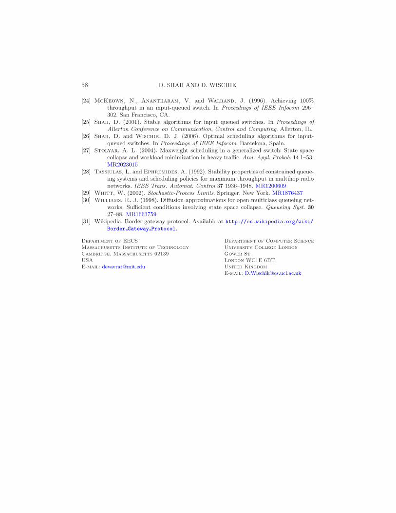
58 D. SHAH AND D. WISCHIK
[24] McKeown, N., Anantharam, V. and Walrand, J. (1996). Achieving 100%throughput in an input-queued switch. In Proceedings of IEEE Infocom 296–302. San Francisco, CA.
[25] Shah, D. (2001). Stable algorithms for input queued switches. In Proceedings ofAllerton Conference on Communication, Control and Computing. Allerton, IL.
[26] Shah, D. and Wischik, D. J. (2006). Optimal scheduling algorithms for input-queued switches. In Proceedings of IEEE Infocom. Barcelona, Spain.
[27] Stolyar, A. L. (2004). Maxweight scheduling in a generalized switch: State spacecollapse and workload minimization in heavy traffic. Ann. Appl. Probab. 14 1–53.MR2023015
[28] Tassiulas, L. and Ephremides, A. (1992). Stability properties of constrained queue-ing systems and scheduling policies for maximum throughput in multihop radionetworks. IEEE Trans. Automat. Control 37 1936–1948. MR1200609
[29] Whitt, W. (2002). Stochastic-Process Limits. Springer, New York. MR1876437[30] Williams, R. J. (1998). Diffusion approximations for open multiclass queueing net-
works: Sufficient conditions involving state space collapse. Queueing Syst. 3027–88. MR1663759
[31] Wikipedia. Border gateway protocol. Available at http://en.wikipedia.org/wiki/Border Gateway Protocol.
Department of EECS
Massachusetts Institute of Technology
Cambridge, Massachusetts 02139
USA
E-mail: [email protected]
Department of Computer Science
University College London
Gower St.
London WC1E 6BT
United Kingdom
E-mail: [email protected]