Embed Size (px)
Citation preview
FLUID FLOWFLUID FLOWBASICSBASICS
O FO FTHROTTLING VALVESTHROTTLING VALVES
01-99
-2-
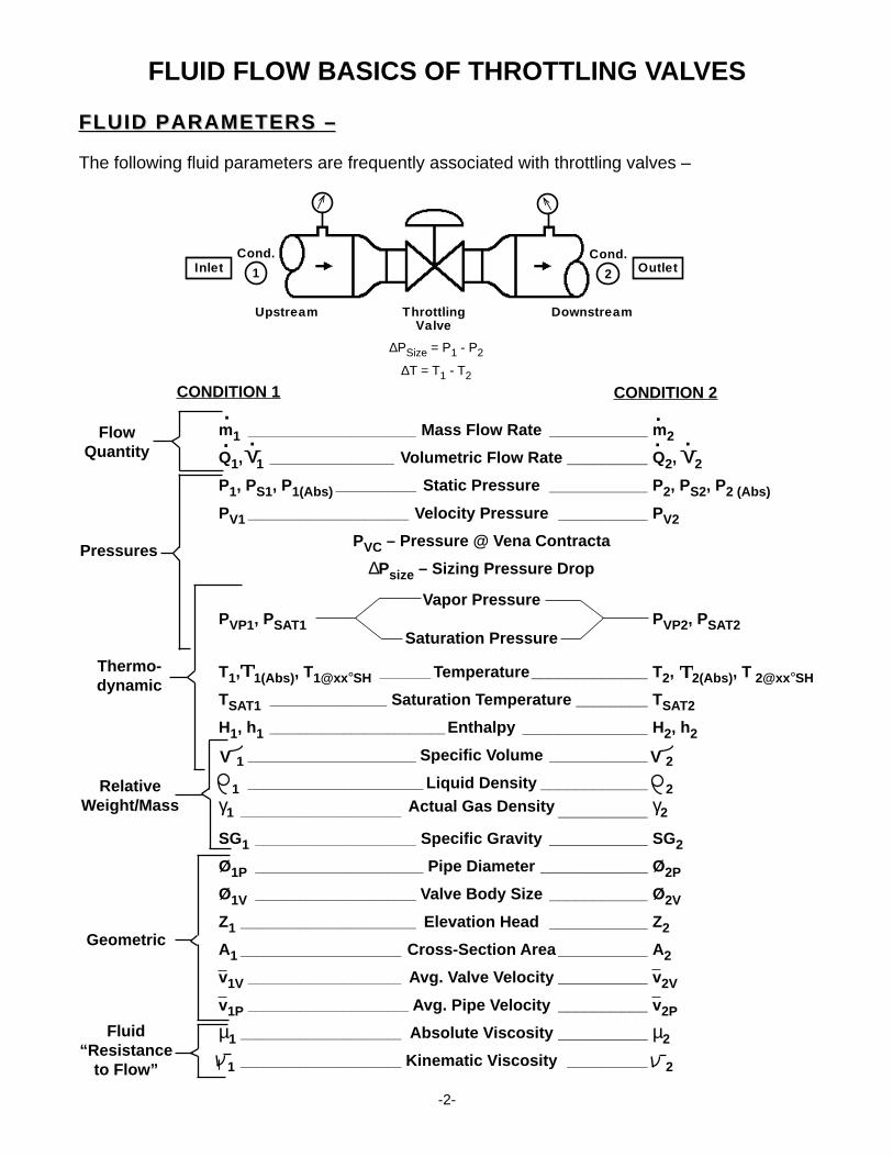
Cond.
1
Cond.
2Inlet Outlet
ThrottlingValve
Upstream Downstream
FLUID FLOW BASICS OF THROTTLING VALVES
FLUID PARAMETERS –FLUID PARAMETERS –
The following fluid parameters are frequently associated with throttling valves –
∆PSize = P1 - P2
∆T = T1 - T2
Pressures
FlowQuantity
Thermo-dynamic
RelativeWeight/Mass
Geometric
Fluid“Resistance
to Flow”
CONDITION 1 CONDITION 2
m1 _______________________ Mass Flow Rate ___________ m 2
Q1, 1 _________________ Volumetric Flow Rate _________ Q 2, 2P1, PS1, P1(Abs) ___________ Static Pressure ___________ P 2, PS2, P2 (Abs)
PV1 ______________________ Velocity Pressure __________ P V2
PVC – Pressure @ Vena Contracta
∆Psize – Sizing Pressure Drop
Vapor PressurePVP1, PSAT1 PVP2, PSAT2
Saturation Pressure
T1, 1(Abs) , T1@xx°SH _______ Temperature_____________ T 2, 2(Abs) , T 2@xx°SH
TSAT1 ________________ Saturation Temperature ________ T SAT2
H1, h1 ________________________ Enthalpy ______________ H 2, h2
1 _______________________ Specific Volume ___________ 2
1 ________________________ Liquid Density ____________ 2γ1 ______________________ Actual Gas Density __________ γ2
SG1 ______________________ Specific Gravity ___________ SG 2
Ø1P _______________________ Pipe Diameter ____________ Ø 2P
Ø1V ______________________ Valve Body Size ___________ Ø 2V
Z1 ________________________ Elevation Head ___________ Z 2
A1 ______________________ Cross-Section Area __________ A 2
v1V _____________________ Avg. Valve Velocity __________ v 2V
v1P ______________________ Avg. Pipe Velocity __________ v 2P
µ1 ______________________ Absolute Viscosity __________ µ2
1 ______________________ Kinematic Viscosity _________ 2
.
. ... .
V V
V V
-3-
Cond.
1
Cond.
2Inlet Outlet
ThrottlingValve
∆P = P - P1 2
Upstream Downstream
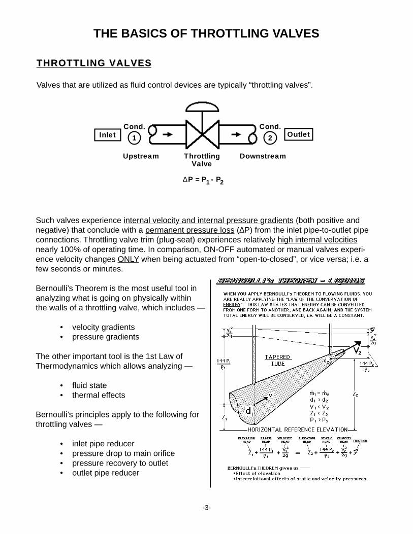
THE BASICS OF THROTTLING VALVES
THROTTLING VALVESTHROTTLING VALVES
Valves that are utilized as fluid control devices are typically “throttling valves”.
Such valves experience internal velocity and internal pressure gradients (both positive andnegative) that conclude with a permanent pressure loss (∆P) from the inlet pipe-to-outlet pipeconnections. Throttling valve trim (plug-seat) experiences relatively high internal velocitiesnearly 100% of operating time. In comparison, ON-OFF automated or manual valves experi-ence velocity changes ONLY when being actuated from “open-to-closed”, or vice versa; i.e. afew seconds or minutes.
Bernoulli’s Theorem is the most useful tool inanalyzing what is going on physically withinthe walls of a throttling valve, which includes —
• velocity gradients• pressure gradients
The other important tool is the 1st Law ofThermodynamics which allows analyzing —
• fluid state• thermal effects
Bernoulli’s principles apply to the following forthrottling valves —
• inlet pipe reducer• pressure drop to main orifice• pressure recovery to outlet• outlet pipe reducer
-4-
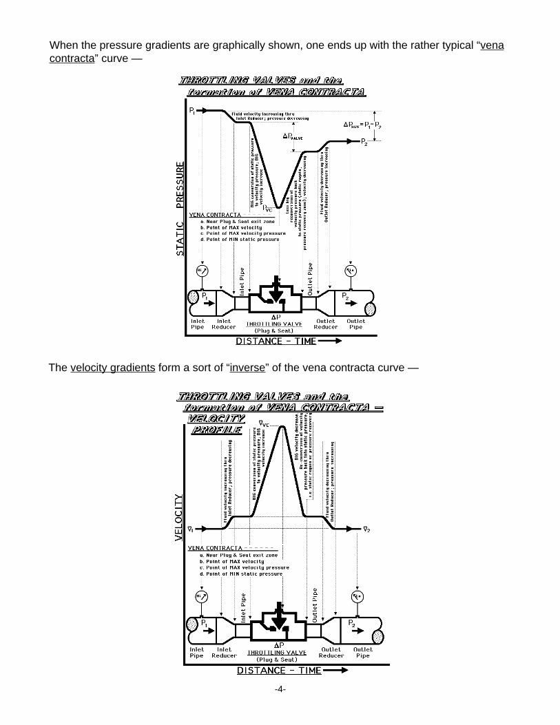
When the pressure gradients are graphically shown, one ends up with the rather typical “venacontracta” curve —
The velocity gradients form a sort of “inverse” of the vena contracta curve —
-5-
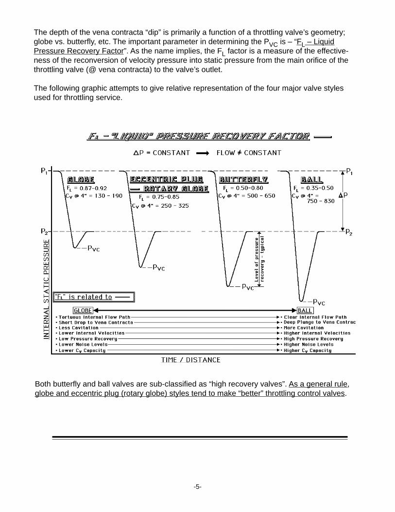
The depth of the vena contracta “dip” is primarily a function of a throttling valve’s geometry;globe vs. butterfly, etc. The important parameter in determining the PVC is – “FL – LiquidPressure Recovery Factor”. As the name implies, the FL factor is a measure of the effective-ness of the reconversion of velocity pressure into static pressure from the main orifice of thethrottling valve (@ vena contracta) to the valve’s outlet.
The following graphic attempts to give relative representation of the four major valve stylesused for throttling service.
Both butterfly and ball valves are sub-classified as “high recovery valves”. As a general rule,globe and eccentric plug (rotary globe) styles tend to make “better” throttling control valves.
-6-
Cond.
1
Cond.
2
ThrottlingValve
Upstream Downstream
LIQUID(Non-Compressible)
GAS–VAPOR(Compressible)
∆P = P1 - P2
LIQUIDLIQUID
FLUID STATESFLUID STATES
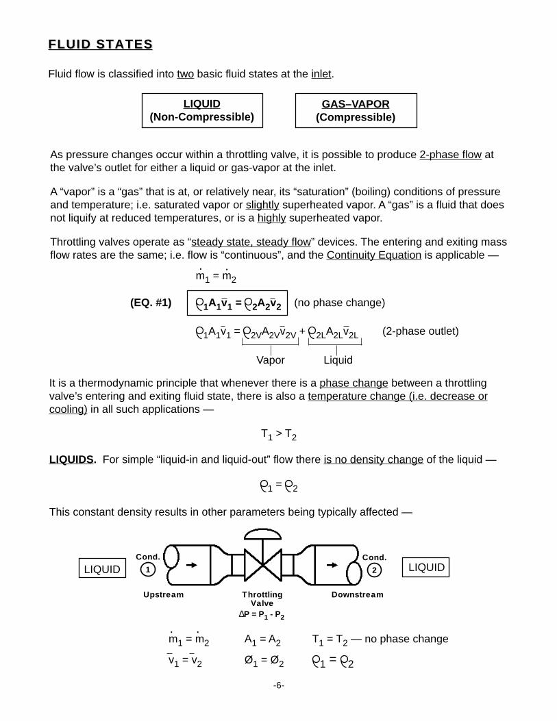
Fluid flow is classified into two basic fluid states at the inlet.
As pressure changes occur within a throttling valve, it is possible to produce 2-phase flow atthe valve’s outlet for either a liquid or gas-vapor at the inlet.
A “vapor” is a “gas” that is at, or relatively near, its “saturation” (boiling) conditions of pressureand temperature; i.e. saturated vapor or slightly superheated vapor. A “gas” is a fluid that doesnot liquify at reduced temperatures, or is a highly superheated vapor.
Throttling valves operate as “steady state, steady flow” devices. The entering and exiting massflow rates are the same; i.e. flow is “continuous”, and the Continuity Equation is applicable —
It is a thermodynamic principle that whenever there is a phase change between a throttlingvalve’s entering and exiting fluid state, there is also a temperature change (i.e. decrease orcooling) in all such applications —
T1 > T2
LIQUIDS. For simple “liquid-in and liquid-out” flow there is no density change of the liquid —
1 = 2
This constant density results in other parameters being typically affected —
. .m1 = m2
(EQ. #1) 1A1v1 = 2A2v2 (no phase change)
1A1v1 = 2VA2Vv2V + 2LA2Lv2L (2-phase outlet)
Vapor Liquid
m1 = m2 A1 = A2 T1 = T2 — no phase change
v1 = v2 Ø1 = Ø2 1 = 2
..
-7-
Cond.
1
Cond.
2Inlet Outlet
ThrottlingValve
Upstream Downstream
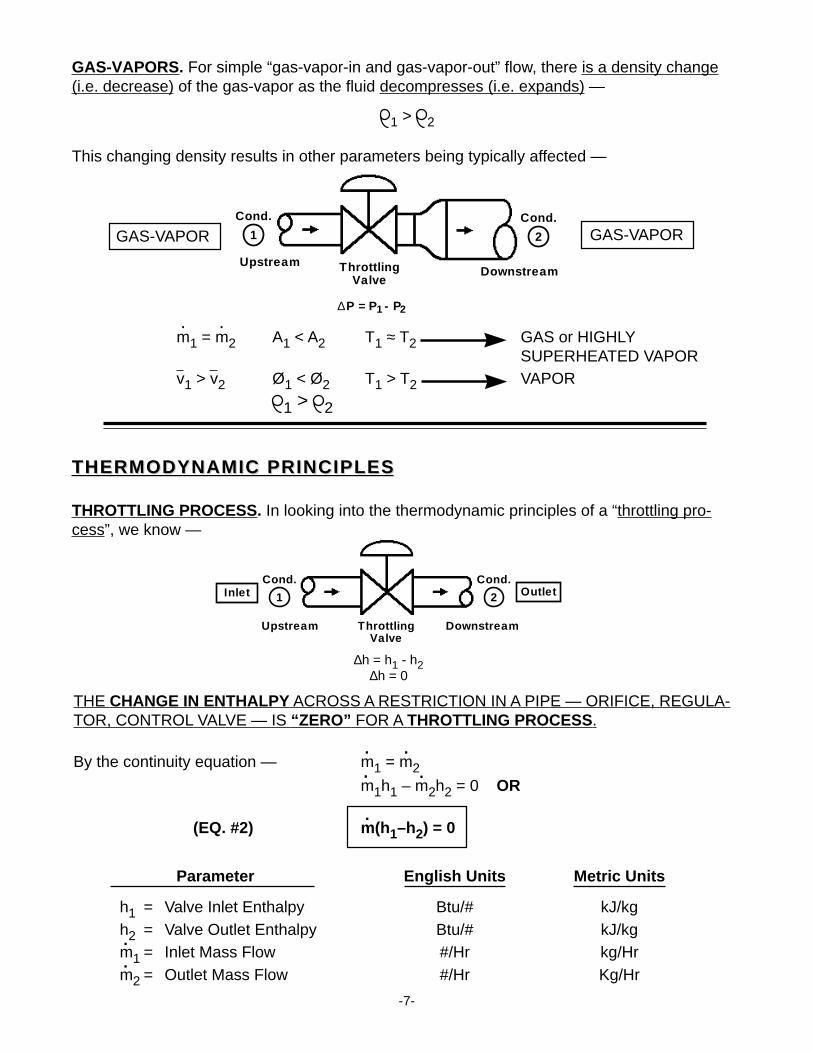
GAS-VAPORS. For simple “gas-vapor-in and gas-vapor-out” flow, there is a density change(i.e. decrease) of the gas-vapor as the fluid decompresses (i.e. expands) —
1 > 2
This changing density results in other parameters being typically affected —
GAS-VAPORGAS-VAPOR
∆h = h1 - h2∆h = 0
THERMODYNAMIC PRINCIPLESTHERMODYNAMIC PRINCIPLES
THROTTLING PROCESS. In looking into the thermodynamic principles of a “throttling pro-cess”, we know —
Cond.
1Cond.
2
ThrottlingValve
∆P = P - P1 2
UpstreamDownstream
.
.
Parameter English Units Metric Units
h1 = Valve Inlet Enthalpy Btu/# kJ/kgh2 = Valve Outlet Enthalpy Btu/# kJ/kgm1 = Inlet Mass Flow #/Hr kg/Hrm2 = Outlet Mass Flow #/Hr Kg/Hr
THE CHANGE IN ENTHALPY ACROSS A RESTRICTION IN A PIPE — ORIFICE, REGULA-TOR, CONTROL VALVE — IS “ZERO” FOR A THROTTLING PROCESS.
By the continuity equation — m1 = m2m1h1 – m2h2 = 0 OR
(EQ. #2) m(h1–h2) = 0
. .
.
.
.
..m1 = m2 A1 < A2 T1 ≈ T2 GAS or HIGHLY
SUPERHEATED VAPORv1 > v2 Ø1 < Ø2 T1 > T2 VAPOR
1 > 2
-8-
It is the use of fluid thermodynamic data and the thermodynamic principles of the “constantenthalpy throttling process” that throttling valves experience which allows an accurate determi-nation of a fluid’s state while internal to the valve as well as at the valve’s outlet. In particular,we want to know what the fluid is physically doing at the throttling valve’s main orifice (plug-seat); i.e. what is occurring at the vena contracta and elsewhere within the valve?
SATURATION STATE. A fluid is said to be “saturated” when —
• Liquid - when at the boiling temperature – Tsat – for a given pressure – PsatExamples: Water @ Psat = 14.7 psia Tsat = 212°F
Psat = 1.0135 BarA Tsat = 100°C
Water @Psat = 145 psig Tsat = 355.8°FPsat = 10 BarA Tsat = 179.9°C
• Vapor - when at the boiling temperature – Tsat – for a given pressure – PsatExamples: Steam @ Psat = 14.7 psia Tsat = 212°F
Psat = 1.0135 BarA Tsat = 100°C
Steam @ Psat = 145 psig Tsat = 355.8°FPsat = 10 BarA Tsat = 179.9°C
Restating the above examples, we have both saturated liquid water (condensate) and satu-rated steam at the same Psat and Tsat. Further, for any given fluid in its “saturation” state, whenwe have its pressure (Psat), we KNOW its temperature (Tsat). To say a fluid is “saturated” is togive a property of the fluid. Only two extensive properties of a fluid will locate the fluid in thephysical universe. We know exactly where a fluid is when we say the fluid is —
• saturated water at Psat = 29 psia = 2.0 BarA, we know that Tsat = 248.4°F = 120.1°C.• saturated steam at Tsat = 212°F = 100°C, we know that Psat = 14.7 psig = 1.013 BarA.
SUPERHEATED VAPOR. A fluid is a superheated vapor when its temperature is greater thanTsat corresponding to the flowing pressure.
Examples: Steam @ P1 = 145 psia & T1 = 425°F69.2°F SH
(Tsat = 355.8°F)
P1 = 10 BarA & T1 = 219°C39.1°C SH
(Tsat = 179.9°C)
-9-
To say a vapor is “superheated” does NOT give an extensive property of the fluid; so, a secondproperty must also be known to physically locate a superheated vapor in the universe.
SUB-COOLED LIQUID . A liquid is sub-cooled when its temperature is less than Tsat corre-sponding to the flowing pressure.
Example: Water @ P = 145 psia & T = 60°F (Tsat = 355.8°F)P = 10 BarA & T = 15.5°C (Tsat = 179.9°C)
To say a liquid is “sub-cooled” is NOT to give an extensive property of the fluid; so, a secondproperty must also be known to physically locate a sub-cooled liquid in the universe.
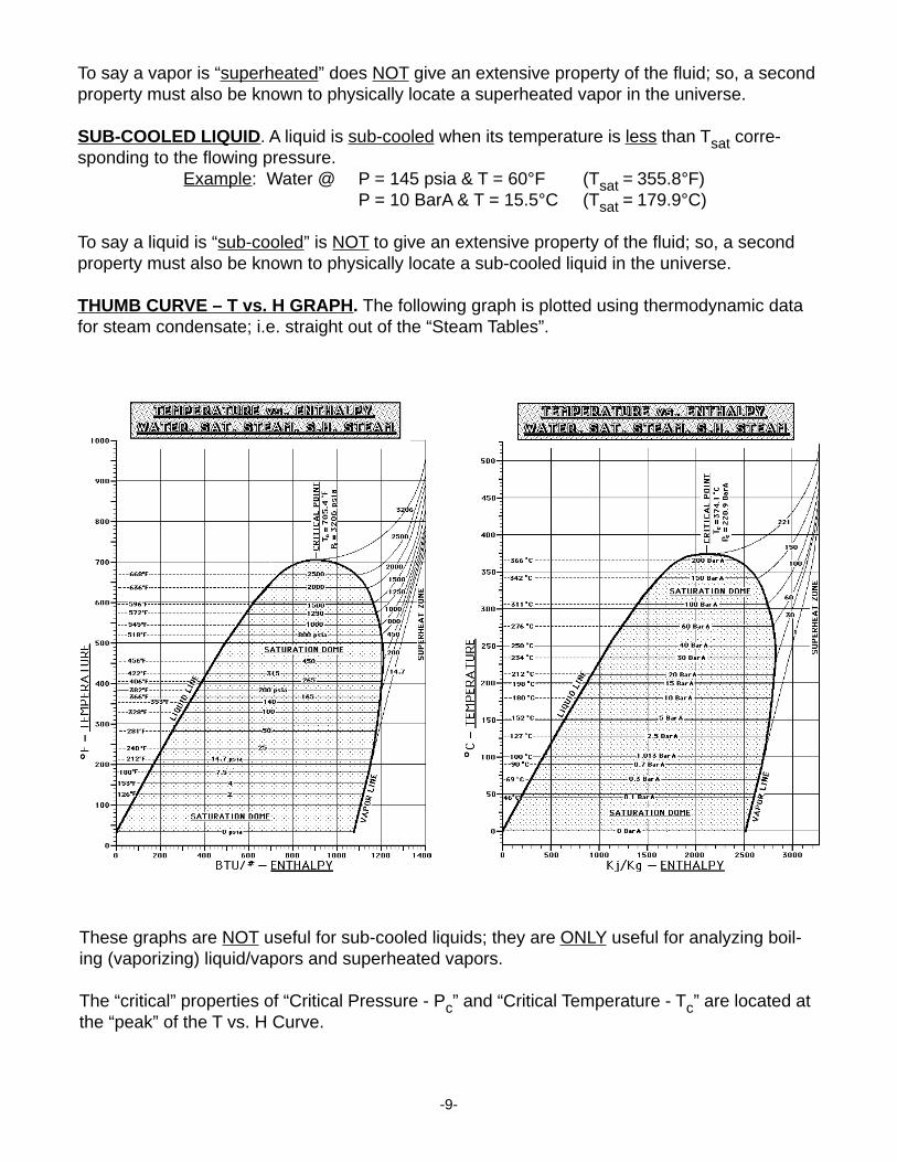
THUMB CURVE – T vs. H GRAPH. The following graph is plotted using thermodynamic datafor steam condensate; i.e. straight out of the “Steam Tables”.
These graphs are NOT useful for sub-cooled liquids; they are ONLY useful for analyzing boil-ing (vaporizing) liquid/vapors and superheated vapors.
The “critical” properties of “Critical Pressure - Pc” and “Critical Temperature - Tc” are located atthe “peak” of the T vs. H Curve.
-10-
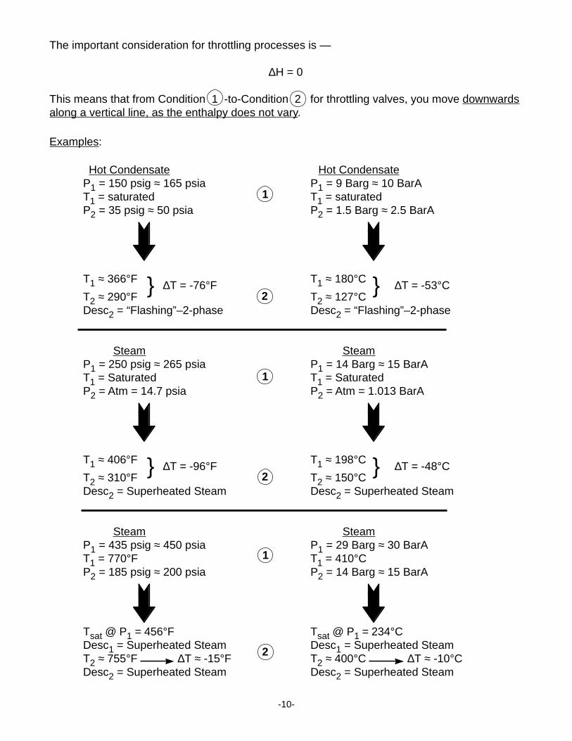
The important consideration for throttling processes is —
∆H = 0
This means that from Condition 1 -to-Condition 2 for throttling valves, you move downwardsalong a vertical line, as the enthalpy does not vary.
Examples:
Hot Condensate Hot CondensateP1 = 150 psig ≈ 165 psia P1 = 9 Barg ≈ 10 BarAT1 = saturated T1 = saturatedP2 = 35 psig ≈ 50 psia P2 = 1.5 Barg ≈ 2.5 BarA
T1 ≈ 366°F } ∆T = -76°F T1 ≈ 180°C } ∆T = -53°CT2 ≈ 290°F T2 ≈ 127°CDesc2 = “Flashing”–2-phase Desc2 = “Flashing”–2-phase
Steam SteamP1 = 250 psig ≈ 265 psia P1 = 14 Barg ≈ 15 BarAT1 = Saturated T1 = SaturatedP2 = Atm = 14.7 psia P2 = Atm = 1.013 BarA
T1 ≈ 406°F } ∆T = -96°F T1 ≈ 198°C } ∆T = -48°CT2 ≈ 310°F T2 ≈ 150°CDesc2 = Superheated Steam Desc2 = Superheated Steam
Steam SteamP1 = 435 psig ≈ 450 psia P1 = 29 Barg ≈ 30 BarAT1 = 770°F T1 = 410°CP2 = 185 psig ≈ 200 psia P2 = 14 Barg ≈ 15 BarA
Tsat @ P1 = 456°F Tsat @ P1 = 234°CDesc1 = Superheated Steam Desc1 = Superheated SteamT2 ≈ 755°F ∆T ≈ -15°F T2 ≈ 400°C ∆T ≈ -10°CDesc2 = Superheated Steam Desc2 = Superheated Steam
2
1
2
1
2
1

-11-
TEMPERATURE. By reviewing the T vs. H Graphs on pg. 9, we can make a few temperaturegeneralizations for saturated steam —
• A throttling ∆T (i.e. T1 – T2) is always present with a throttling ∆P (i.e. P1 – P2).• Greater ∆T’s occur for throttling ∆P’s within the saturation dome.• A ∆T is always associated with a throttling ∆P that causes phase change.• Highly superheated vapor has a relatively small ∆T for a throttling ∆P.• Slightly superheated vapor has a higher ∆T for a throttling ∆P than a highly super-
heated vapor.• Vapors carry higher “heat contents”.
This cooling effect due to throttling is frequently referred to as “Joule-Thompson cooling”.
When a liquid is sub-cooled (below Tsat) both in and out of a throttling valve —
• There is no ∆T (i.e. T1 = T2) for a throttling ∆P.
BASIC PRINCIPLES . If one learns thethermodynamic principles of water-steam, then the same principles can beapplied to many other fluids, even thosethat typically exist as gas-vapor at ambi-ent pressure and temperature conditions.A basic understanding of these principleswill help in understanding the processindustry, because fluid separation bydiffering boiling points is a commonoccurrence in the Chemical ProcessIndustry. Notice the similarity of thesaturation domes of butane, propane,ethane, and methane plotted together atright; there is a striking resemblance tothe earlier water-steam H vs. T plot. Asvery few processes operate at ambientpressures, one must be aware of the“pressure” conditions as well as the“temperature” conditions TOGETHER;i.e. Tsat & Psat. Air separation plants andcrude oil distillation processes are ex-amples of application of these principles.
For throttling valves, an understanding ofthese principles will help in understand-ing both “Cavitation” and “Flashing” in the liquid flow realm, and will also help with understand-ing refrigeration and cryogenic applications.
-12-
NRep = D•V•No•µ
(EQ #3)
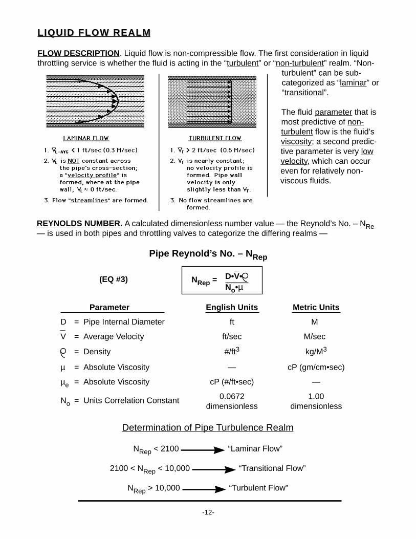
LIQUID FLOW REALMLIQUID FLOW REALM
FLOW DESCRIPTION. Liquid flow is non-compressible flow. The first consideration in liquidthrottling service is whether the fluid is acting in the “turbulent” or “non-turbulent” realm. “Non-
turbulent” can be sub-categorized as “laminar” or“transitional”.
The fluid parameter that ismost predictive of non-turbulent flow is the fluid’sviscosity; a second predic-tive parameter is very lowvelocity, which can occureven for relatively non-viscous fluids.
REYNOLDS NUMBER. A calculated dimensionless number value — the Reynold’s No. – NRe— is used in both pipes and throttling valves to categorize the differing realms —
Pipe Reynold’s No. – N Rep
Parameter English Units Metric Units
D = Pipe Internal Diameter ft M
V = Average Velocity ft/sec M/sec
= Density #/ft3 kg/M3
µ = Absolute Viscosity — cP (gm/cm•sec)
µe = Absolute Viscosity cP (#/ft•sec) —
No = Units Correlation Constant 0.0672 1.00dimensionless dimensionless
Determination of Pipe Turbulence Realm
NRep < 2100 “Laminar Flow”
2100 < NRep < 10,000 “Transitional Flow”
NRep > 10,000 “Turbulent Flow”
-13-
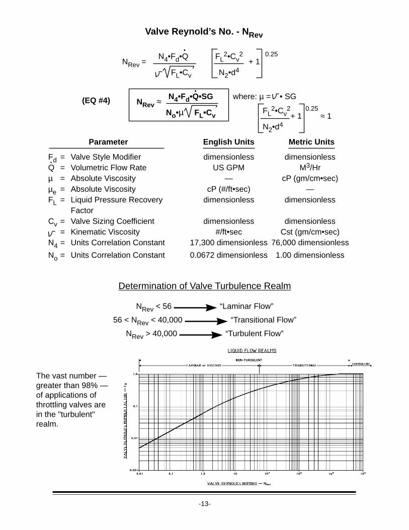
Valve Reynold’s No. - N Rev
NRev =N4•Fd•Q FL
2•Cv2
+ 10.25
FL•Cv N2•d4
.
(EQ #4) NRev ≈ N4•Fd•Q•SG where: µ = • SG
No•µ FL•Cv
.
FL2•Cv
2+ 1
0.25 ≈ 1
N2•d4
Parameter English Units Metric Units
Fd = Valve Style Modifier dimensionless dimensionlessQ = Volumetric Flow Rate US GPM M3/Hrµ = Absolute Viscosity — cP (gm/cm•sec)µe = Absolute Viscosity cP (#/ft•sec) —FL = Liquid Pressure Recovery dimensionless dimensionless
FactorCv = Valve Sizing Coefficient dimensionless dimensionless
= Kinematic Viscosity #/ft•sec Cst (gm/cm•sec)N4 = Units Correlation Constant 17,300 dimensionless 76,000 dimensionless
No = Units Correlation Constant 0.0672 dimensionless 1.00 dimensionless
Determination of Valve Turbulence Realm
NRev < 56 “Laminar Flow”
56 < NRev < 40,000 “Transitional Flow”
NRev > 40,000 “Turbulent Flow”
The vast number —greater than 98% —of applications ofthrottling valves arein the "turbulent"realm.
.
-14-
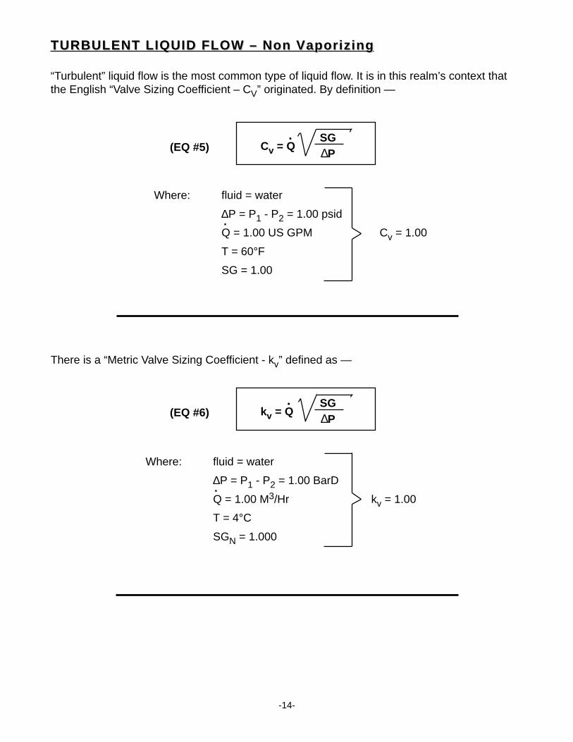
TURBULENT LIQUID FLOW – Non VaporizingTURBULENT LIQUID FLOW – Non Vaporizing
“Turbulent” liquid flow is the most common type of liquid flow. It is in this realm’s context thatthe English “Valve Sizing Coefficient – CV” originated. By definition —
There is a “Metric Valve Sizing Coefficient - kv” defined as —
.
(EQ #5) Cv = QSG∆P
.
Where: fluid = water
∆P = P1 - P2 = 1.00 psid
Q = 1.00 US GPM Cv = 1.00
T = 60°F
SG = 1.00
(EQ #6) kv = QSG∆P
.
Where: fluid = water
∆P = P1 - P2 = 1.00 BarD
Q = 1.00 M3/Hr kv = 1.00
T = 4°C
SGN = 1.000
.
-15-
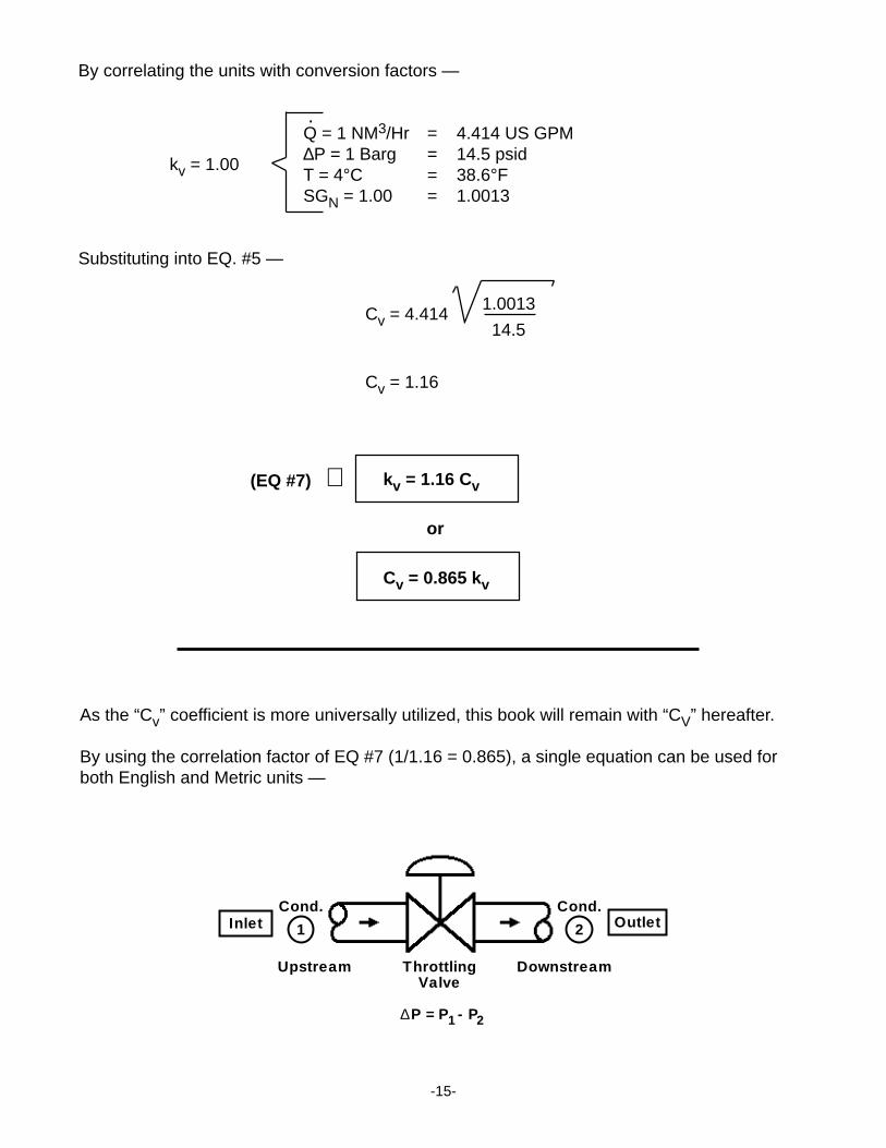
As the “Cv” coefficient is more universally utilized, this book will remain with “CV” hereafter.
By using the correlation factor of EQ #7 (1/1.16 = 0.865), a single equation can be used forboth English and Metric units —
Cond.
1
Cond.
2Inlet Outlet
ThrottlingValve
∆P = P - P1 2
Upstream Downstream
By correlating the units with conversion factors —
Q = 1 NM3/Hr = 4.414 US GPM
kv = 1.00∆P = 1 Barg = 14.5 psidT = 4°C = 38.6°FSGN = 1.00 = 1.0013
Substituting into EQ. #5 —
Cv = 4.4141.0013
14.5
Cv = 1.16
.
(EQ #7) kv = 1.16 Cv
or
Cv = 0.865 kv
∴
-16-
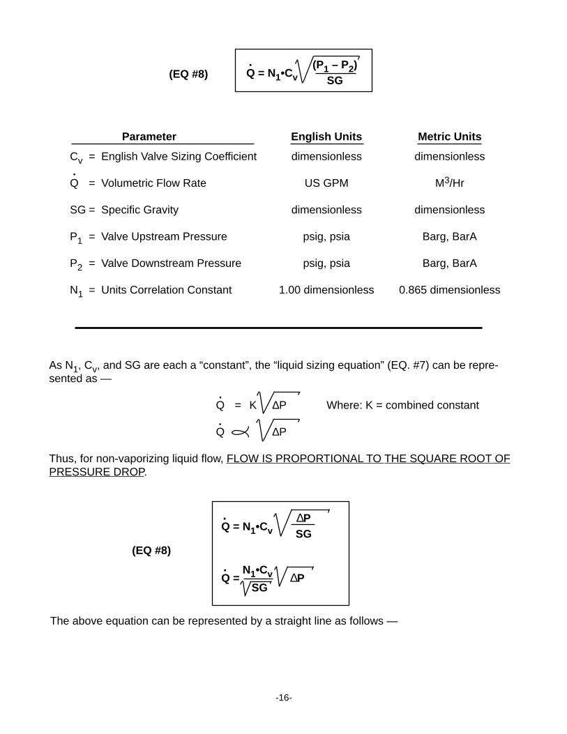
The above equation can be represented by a straight line as follows —
(EQ #8) Q = N1•Cv(P1 – P2)
SG
.
Parameter English Units Metric Units
Cv = English Valve Sizing Coefficient dimensionless dimensionless
Q = Volumetric Flow Rate US GPM M3/Hr
SG = Specific Gravity dimensionless dimensionless
P1 = Valve Upstream Pressure psig, psia Barg, BarA
P2 = Valve Downstream Pressure psig, psia Barg, BarA
N1 = Units Correlation Constant 1.00 dimensionless 0.865 dimensionless
.
As N1, Cv, and SG are each a “constant”, the “liquid sizing equation” (EQ. #7) can be repre-sented as —
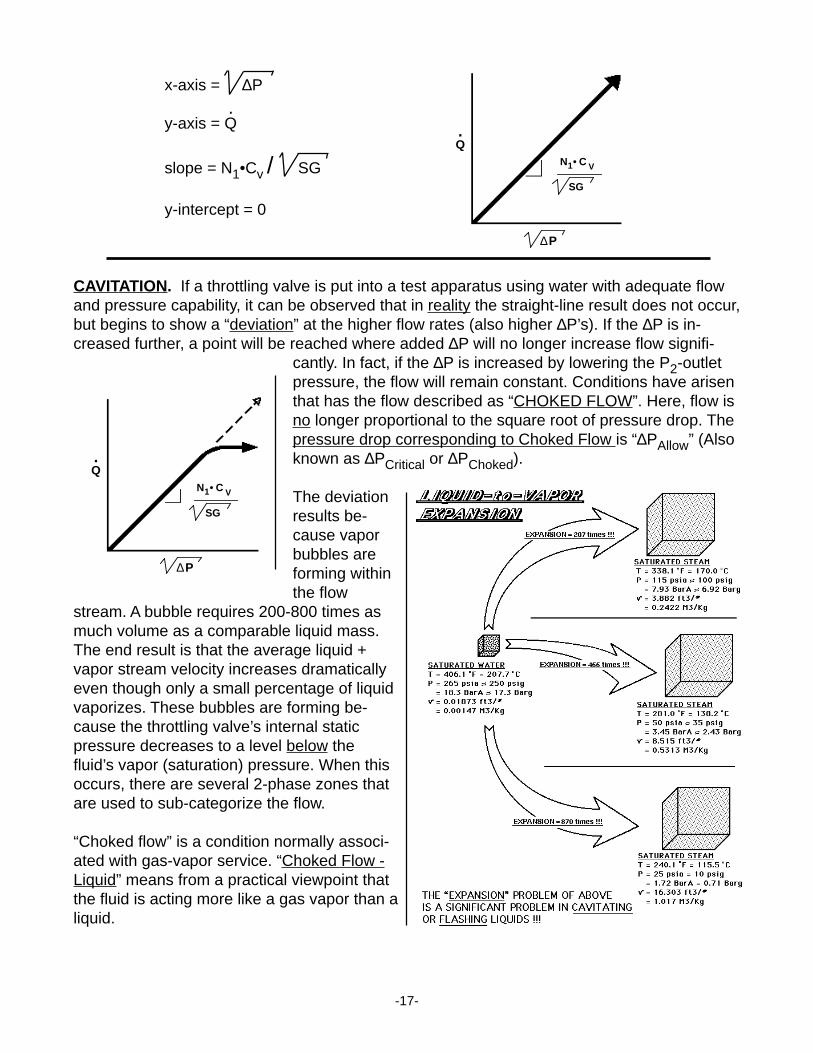
Q = K ∆P Where: K = combined constant
Q ∆P
Thus, for non-vaporizing liquid flow, FLOW IS PROPORTIONAL TO THE SQUARE ROOT OFPRESSURE DROP.
.
.
Q = N1•Cv∆PSG
Q = N1•Cv ∆P
SG
(EQ #8)
.
.
-17-
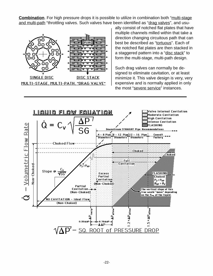
CAVITATION. If a throttling valve is put into a test apparatus using water with adequate flowand pressure capability, it can be observed that in reality the straight-line result does not occur,but begins to show a “deviation” at the higher flow rates (also higher ∆P’s). If the ∆P is in-creased further, a point will be reached where added ∆P will no longer increase flow signifi-
cantly. In fact, if the ∆P is increased by lowering the P2-outletpressure, the flow will remain constant. Conditions have arisenthat has the flow described as “CHOKED FLOW”. Here, flow isno longer proportional to the square root of pressure drop. Thepressure drop corresponding to Choked Flow is “∆PAllow” (Alsoknown as ∆PCritical or ∆PChoked).
The deviationresults be-cause vaporbubbles areforming withinthe flow
stream. A bubble requires 200-800 times asmuch volume as a comparable liquid mass.The end result is that the average liquid +vapor stream velocity increases dramaticallyeven though only a small percentage of liquidvaporizes. These bubbles are forming be-cause the throttling valve’s internal staticpressure decreases to a level below thefluid’s vapor (saturation) pressure. When thisoccurs, there are several 2-phase zones thatare used to sub-categorize the flow.
“Choked flow” is a condition normally associ-ated with gas-vapor service. “Choked Flow -Liquid” means from a practical viewpoint thatthe fluid is acting more like a gas vapor than aliquid.
N • C1 V
SG
∆P
Q.
N • C1 V
SG
∆P
Q.
x-axis = ∆P
y-axis = Q
slope = N1•Cv / SG
y-intercept = 0
.
-18-
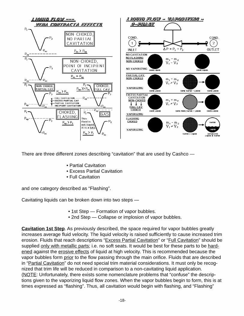
There are three different zones describing “cavitation” that are used by Cashco —
• Partial Cavitation• Excess Partial Cavitation• Full Cavitation
and one category described as “Flashing”.
Cavitating liquids can be broken down into two steps —
• 1st Step — Formation of vapor bubbles.• 2nd Step — Collapse or implosion of vapor bubbles.
Cavitation 1st Step . As previously described, the space required for vapor bubbles greatlyincreases average fluid velocity. The liquid velocity is raised sufficiently to cause increased trimerosion. Fluids that reach descriptions “Excess Partial Cavitation” or “Full Cavitation” should besupplied only with metallic parts; i.e. no soft seats. It would be best for these parts to be hard-ened against the erosive effects of liquid at high velocity. This is recommended because thevapor bubbles form prior to the flow passing through the main orifice. Fluids that are describedin “Partial Cavitation” do not need special trim material considerations. It must only be recog-nized that trim life will be reduced in comparison to a non-cavitating liquid application.(NOTE: Unfortunately, there exists some nomenclature problems that “confuse” the descrip-tions given to the vaporizing liquid flow zones. When the vapor bubbles begin to form, this is attimes expressed as “flashing”. Thus, all cavitation would begin with flashing, and “Flashing”
-19-
would also begin and end with “flashing”. This book will ONLY use “Flashing” to describe theliquid zone where P2 < PVP, and the outlet of valve and pipe will contain permanent 2-phaseflow.)
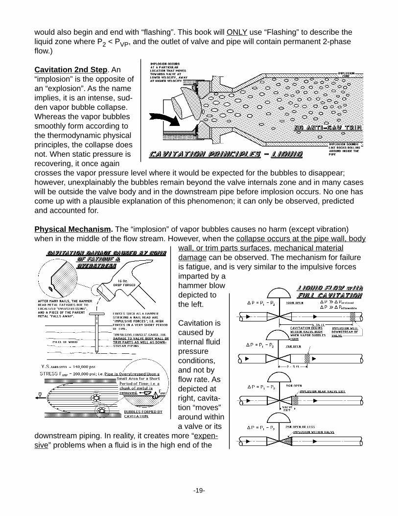
Cavitation 2nd Step . An“implosion” is the opposite ofan “explosion”. As the nameimplies, it is an intense, sud-den vapor bubble collapse.Whereas the vapor bubblessmoothly form according tothe thermodynamic physicalprinciples, the collapse doesnot. When static pressure isrecovering, it once againcrosses the vapor pressure level where it would be expected for the bubbles to disappear;however, unexplainably the bubbles remain beyond the valve internals zone and in many caseswill be outside the valve body and in the downstream pipe before implosion occurs. No one hascome up with a plausible explanation of this phenomenon; it can only be observed, predictedand accounted for.
Physical Mechanism. The “implosion” of vapor bubbles causes no harm (except vibration)when in the middle of the flow stream. However, when the collapse occurs at the pipe wall, body
wall, or trim parts surfaces, mechanical materialdamage can be observed. The mechanism for failureis fatigue, and is very similar to the impulsive forcesimparted by ahammer blowdepicted tothe left.
Cavitation iscaused byinternal fluidpressureconditions,and not byflow rate. Asdepicted atright, cavita-tion “moves”around withina valve or its
downstream piping. In reality, it creates more “expen-sive” problems when a fluid is in the high end of the
-20-
“Excess Partial Cavitation” zone or barely into the “Full Cavitation” zone, for the implosion caneasily occur within the valve body, leading to premature valve “problems” —
• body wall is penetrated • packing leaks• trim is eroded • diaphragms fail• guides and bearings become worn • soft seats fail.
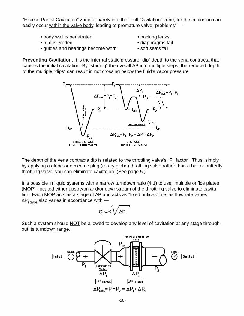
Preventing Cavitation. It is the internal static pressure “dip” depth to the vena contracta thatcauses the initial cavitation. By “staging” the overall ∆P into multiple steps, the reduced depthof the multiple “dips” can result in not crossing below the fluid’s vapor pressure.
The depth of the vena contracta dip is related to the throttling valve’s “FL factor”. Thus, simplyby applying a globe or eccentric plug (rotary globe) throttling valve rather than a ball or butterflythrottling valve, you can eliminate cavitation. (See page 5.)
It is possible in liquid systems with a narrow turndown ratio (4:1) to use “multiple orifice plates(MOP)” located either upstream and/or downstream of the throttling valve to eliminate cavita-tion. Each MOP acts as a stage of ∆P and acts as “fixed orifices”; i.e. as flow rate varies,∆Pstage also varies in accordance with —
Q ∆P
Such a system should NOT be allowed to develop any level of cavitation at any stage through-out its turndown range.
.
-21-
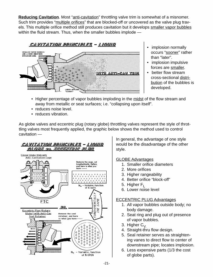
Reducing Cavitation . Most “anti-cavitation” throttling valve trim is somewhat of a misnomer.Such trim provides “multiple orifices” that are blocked-off or uncovered as the valve plug trav-els. This multiple orifice method still produces cavitation but it develops smaller vapor bubbleswithin the fluid stream. Thus, when the smaller bubbles implode —
• implosion normallyoccurs “sooner” ratherthan “later”.
• implosion impulsiveforces are smaller.
• better flow streamcross-sectional distri-bution of the bubbles isdeveloped.
• Higher percentage of vapor bubbles imploding in the midst of the flow stream andaway from metallic or seat surfaces; i.e. “collapsing upon itself”.
• reduces noise level.• reduces vibration.
As globe valves and eccentric plug (rotary globe) throttling valves represent the style of throt-tling valves most frequently applied, the graphic below shows the method used to controlcavitation —
In general, the advantage of one stylewould be the disadvantage of the otherstyle.
GLOBE Advantages1. Smaller orifice diameters2. More orifices3. Higher rangeability4. Better orifice “block-off”5. Higher FL6. Lower noise level
ECCENTRIC PLUG Advantages1. All vapor bubbles outside body; no
body damage.2. Seat ring and plug out of presence
of vapor bubbles.3. Higher CV.4. Straight-thru flow design.5. Seal retainer serves as straighten-
ing vanes to direct flow to center ofdownstream pipe; locates implosion.
6. Less expensive parts (1/3 the costof globe parts).
-22-
Combination . For high pressure drops it is possible to utilize in combination both “multi-stageand multi-path “throttling valves. Such valves have been identified as “drag valves”, and usu-
ally consist of notched flat plates that havemultiple channels milled within that take adirection changing circuitous path that canbest be described as “tortuous”. Each ofthe notched flat plates are then stacked ina staggered pattern into a “disc stack” toform the multi-stage, multi-path design.
Such drag valves can normally be de-signed to eliminate cavitation, or at leastminimize it. This valve design is very, veryexpensive and is normally applied in onlythe most “severe service” instances.
-23-
PARTIAL CAVITATION. As shown in the graphics on pages 18 and 22, the “intensity” of thevapor bubble collapse is not so high as to create serious internal mechanical damage, nor isthe percentage of fluid mass that converts to vapor high enough to significantly effect the flowrate passed through the throttling valve. A “partially cavitating liquid” is further described as“Non-Choked”. There is no special sizing equation that is used for partially cavitating liquidservice. The ∆P to cause the “beginning of cavitation (i.e. point of incipient cavitation)” isknown as ∆PIncip.
FULL CAVITATION. As shown in the graphics on pages 18 and 22, the “intensity” of the vaporbubble collapse is high enough to create very serious internal mechanical damage to thethrottling valve and its downstream piping. The percentage of fluid mass that converts to vaporis high enough to dominate the flow stream, “choking” the flow at the throttling valve’s mainorifice. This level of cavitation is called “Full Cavitation, Choked Flow”. As long as the throttling∆P > 50 psig (3.5 BarD), throttling valves experiencing such cavitation should be —
• Equipped with “anti-cavitation” trim to reduce cavitation intensity.• Equipped with drag valve trim to eliminate cavitation.• Change ∆PThrottle conditions.• Incorporate hardened trim.
The ∆P to cause full cavitation is identified as ∆PAllow.
EXCESS PARTIAL CAVITATION. It is common sense to expect that as flow that is partiallycavitating, but not yet choked, nears full cavitation and choked conditions, such flow could benearly as damaging as full cavitation because —
• internal velocities are very high.• implosion would be more likely to occur within the throttling valve.
Cashco has opted to introduce another level of cavitation intensity identified as “Excess PartialCavitation”. Both ∆PIncip and ∆PAllow can be mathematically calculated. Thus the two empiricalvalues can be subtracted —
∆∆P = ∆PAllow - ∆PIncip
Cashco uses the number of 30% of the ∆∆P as a break point between “Partial Cavitation” and“Excess Partial Cavitation”. Thus, the zones of cavitation separate as follows —
• Non-choked, Partial Cavitation (0.0–30% ∆∆P).• Non-choked, Excess Partial Cavitation (30.1%–99.9% ∆∆P).• Choked, Full Cavitation (∆PActual ≥ ∆PAllow).
Valves experiencing “Excess Partial Cavitation” should be considered for applying anti-cavitational throttling valve trim. This is a “judgement call”; if ∆PActual is greater than 65% ∆∆Plevel, anti-cav trim is recommended.
-24-
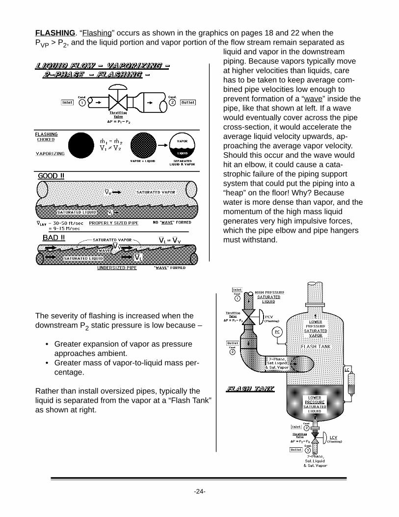
FLASHING . “Flashing” occurs as shown in the graphics on pages 18 and 22 when thePVP > P2, and the liquid portion and vapor portion of the flow stream remain separated as
liquid and vapor in the downstreampiping. Because vapors typically moveat higher velocities than liquids, carehas to be taken to keep average com-bined pipe velocities low enough toprevent formation of a “wave” inside thepipe, like that shown at left. If a wavewould eventually cover across the pipecross-section, it would accelerate theaverage liquid velocity upwards, ap-proaching the average vapor velocity.Should this occur and the wave wouldhit an elbow, it could cause a cata-strophic failure of the piping supportsystem that could put the piping into a“heap” on the floor! Why? Becausewater is more dense than vapor, and themomentum of the high mass liquidgenerates very high impulsive forces,which the pipe elbow and pipe hangersmust withstand.
The severity of flashing is increased when thedownstream P2 static pressure is low because –
• Greater expansion of vapor as pressureapproaches ambient.
• Greater mass of vapor-to-liquid mass per-centage.
Rather than install oversized pipes, typically theliquid is separated from the vapor at a “Flash Tank”as shown at right.
-25-
LIQUID SIZING EQUATIONSLIQUID SIZING EQUATIONS — —
NON-TURBULENT FLOW. The following equations are used for “laminar” or “transitional” flowrealms —
Parameter English Units Metric Units
Cv = English Valve Sizing Coefficient dimensionless dimensionless
Q = Volumetric Flow Rate US GPM M3/Hr
SG = Specific Gravity dimensionless dimensionless
P1 = Valve Upstream Pressure psig, psia Barg, BarA
P2 = Valve Downstream Pressure psig, psia Barg, BarA
N1 = Units Correlation Constant 1.00 dimensionless 0.865 dimensionless
FR = Reynolds No. Correction Factor dimensionless dimensionless
FR can be determined from the graphic on page 13.
There is no known scientific method to evaluate the pipe reducer effect for non-turbulent flow.Thus, the pipe reducer effect is neglected.
TURBULENT FLOW, NON-CHOKED. This is the basic liquid flow equation —
.
(EQ #9) Q = N1•FR• CV
(P1 – P2)SG
.
(EQ #8- repeated) Q = N1• Cv(P1 – P2)
(No pipe reducers)SG
.
(EQ #10) Q = N1• FP• Cv(P1 – P2) (With pipe reducers)
SG
.
Parameter English Units Metric Units
Cv = English Valve Sizing Coefficient dimensionless dimensionless
Q = Volumetric Flow Rate US GPM M3/Hr
SG = Specific Gravity dimensionless dimensionless
P1 = Valve Upstream Pressure psig, psia Barg, BarA
P2 = Valve Downstream Pressure psig, psia Barg, BarA
N1 = Units Correlation Constant 1.00 dimensionless 0.865 dimensionless
FP = Pipe Reducer Effect dimensionless dimensionless
.
-26-
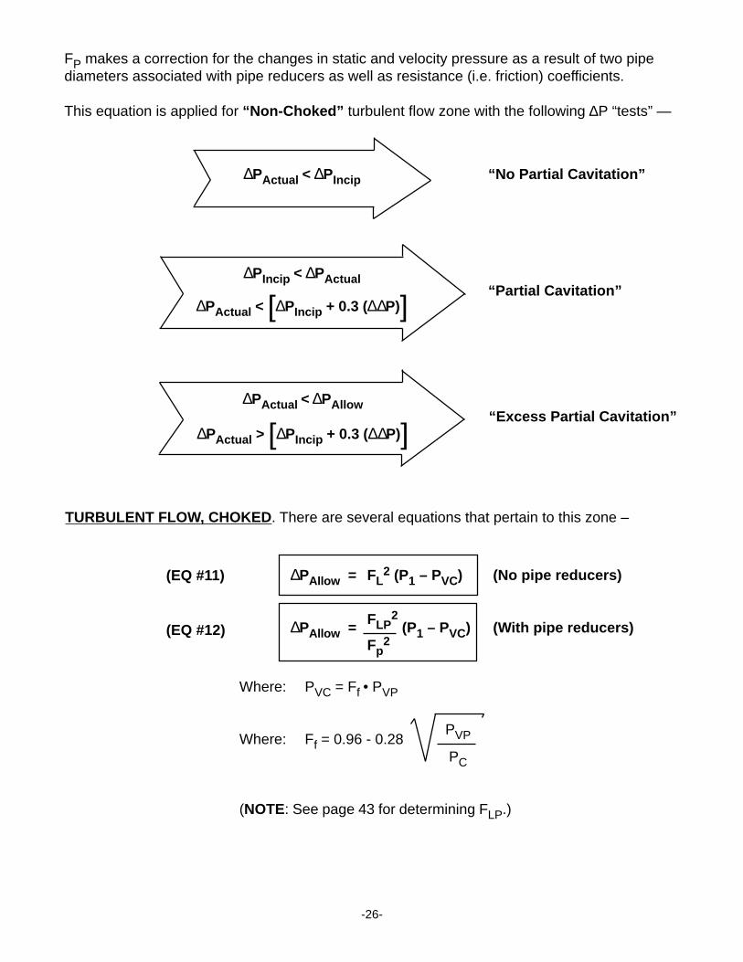
FP makes a correction for the changes in static and velocity pressure as a result of two pipediameters associated with pipe reducers as well as resistance (i.e. friction) coefficients.
This equation is applied for “Non-Choked” turbulent flow zone with the following ∆P “tests” —
TURBULENT FLOW, CHOKED. There are several equations that pertain to this zone –
∆PIncip < ∆PActual“Partial Cavitation”
∆PActual < [∆PIncip + 0.3 (∆∆P)]
∆PActual < ∆PIncip “No Partial Cavitation”
∆PActual < ∆PAllow“Excess Partial Cavitation”
∆PActual > [∆PIncip + 0.3 (∆∆P)]
(EQ #11) ∆PAllow = FL2 (P1 – PVC) (No pipe reducers)
∆PAllow = FLP2 (P1 – PVC) (With pipe reducers)
Fp2
(EQ #12)
Where: PVC = Ff • PVP
Where: Ff = 0.96 - 0.28PVP
PC
(NOTE: See page 43 for determining FLP.)
-27-
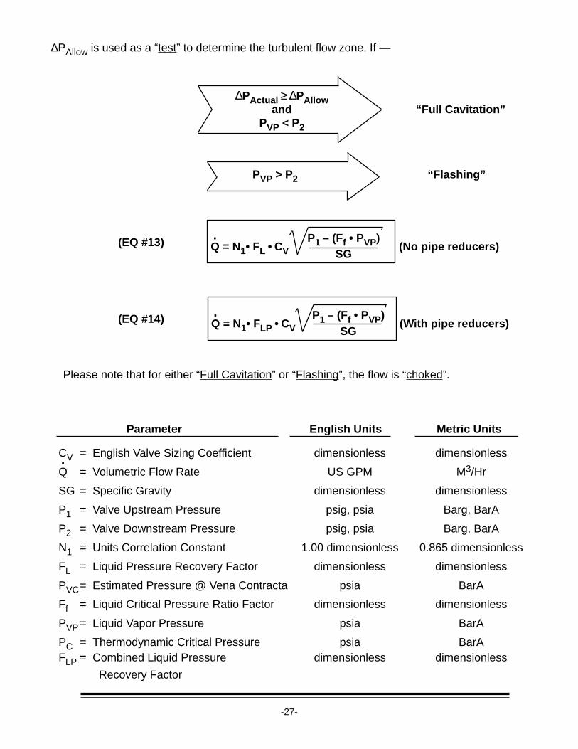
∆PAllow is used as a “test” to determine the turbulent flow zone. If —
∆PActual ≥ ∆PAllowand “Full Cavitation”
PVP < P2
PVP > P2 “Flashing”
(EQ #13) Q = N1• FL • CVP1 – (Ff • PVP)
(No pipe reducers)SG
.
(EQ #14) Q = N1• FLP • CVP1 – (Ff • PVP)
(With pipe reducers)SG
.
Please note that for either “Full Cavitation” or “Flashing”, the flow is “choked”.
Parameter English Units Metric Units
CV = English Valve Sizing Coefficient dimensionless dimensionless
Q = Volumetric Flow Rate US GPM M3/Hr
SG = Specific Gravity dimensionless dimensionless
P1 = Valve Upstream Pressure psig, psia Barg, BarA
P2 = Valve Downstream Pressure psig, psia Barg, BarA
N1 = Units Correlation Constant 1.00 dimensionless 0.865 dimensionless
FL = Liquid Pressure Recovery Factor dimensionless dimensionless
PVC= Estimated Pressure @ Vena Contracta psia BarA
Ff = Liquid Critical Pressure Ratio Factor dimensionless dimensionless
PVP= Liquid Vapor Pressure psia BarA
PC = Thermodynamic Critical Pressure psia BarAFLP = Combined Liquid Pressure dimensionless dimensionless
Recovery Factor
.
-28-
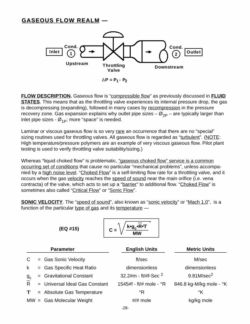
GASEOUS FLOW REALMGASEOUS FLOW REALM — —
FLOW DESCRIPTION. Gaseous flow is “compressible flow” as previously discussed in FLUIDSTATES. This means that as the throttling valve experiences its internal pressure drop, the gasis decompressing (expanding), followed in many cases by recompression in the pressurerecovery zone. Gas expansion explains why outlet pipe sizes – Ø2P – are typically larger thaninlet pipe sizes - Ø1P; more “space” is needed.
Laminar or viscous gaseous flow is so very rare an occurrence that there are no “special”sizing routines used for throttling valves. All gaseous flow is regarded as “turbulent”. (NOTE:High temperature/pressure polymers are an example of very viscous gaseous flow. Pilot planttesting is used to verify throttling valve suitability/sizing.)
Whereas “liquid choked flow” is problematic, “gaseous choked flow” service is a commonoccurring set of conditions that cause no particular “mechanical problems”, unless accompa-nied by a high noise level. “Choked Flow” is a self-limiting flow rate for a throttling valve, and itoccurs when the gas velocity reaches the speed of sound near the main orifice (i.e. venacontracta) of the valve, which acts to set up a “barrier” to additional flow. “Choked Flow” issometimes also called “Critical Flow” or “Sonic Flow”.
SONIC VELOCITY. The “speed of sound”, also known as “sonic velocity” or “Mach 1.0”, is afunction of the particular type of gas and its temperature —
Cond.
1Cond.
2Inlet Outlet
ThrottlingValve
∆P = P - P1 2
UpstreamDownstream
(EQ #15) C =k•gc•R•
MW
Parameter English Units Metric Units
C = Gas Sonic Velocity ft/sec M/sec
k = Gas Specific Heat Ratio dimensionless dimensionless
gc = Gravitational Constant 32.2#m - ft/#f-Sec 2 9.81M/sec2
R = Universal Ideal Gas Constant 1545#f - ft/# mole - °R 846.8 kg-M/kg mole - °K
= Absolute Gas Temperature °R °K
MW = Gas Molecular Weight #/# mole kg/kg mole
-29-
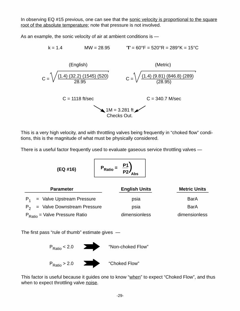
Parameter English Units Metric Units
P1 = Valve Upstream Pressure psia BarA
P2 = Valve Downstream Pressure psia BarA
PRatio = Valve Pressure Ratio dimensionless dimensionless
The first pass “rule of thumb” estimate gives —
PRatio < 2.0 “Non-choked Flow”
PRatio > 2.0 “Choked Flow”
This factor is useful because it guides one to know “when” to expect “Choked Flow”, and thuswhen to expect throttling valve noise.
In observing EQ #15 previous, one can see that the sonic velocity is proportional to the squareroot of the absolute temperature; note that pressure is not involved.
As an example, the sonic velocity of air at ambient conditions is —
k = 1.4 MW = 28.95 = 60°F = 520°R = 289°K = 15°C
(English) (Metric)
C =(1.4) (32.2) (1545) (520)
C =(1.4) (9.81) (846.8) (289)
28.95 (28.95)
C = 1118 ft/sec C = 340.7 M/sec
1M = 3.281 ftChecks Out.
This is a very high velocity, and with throttling valves being frequently in “choked flow” condi-tions, this is the magnitude of what must be physically considered.
There is a useful factor frequently used to evaluate gaseous service throttling valves —
(EQ #16) PRatio = P1P2 Abs)
-30-
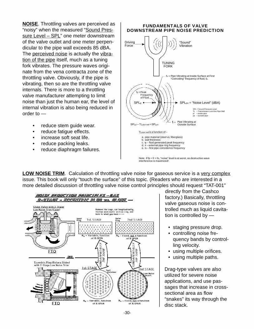
NOISE. Throttling valves are perceived as“noisy” when the measured “Sound Pres-sure Level – SPL” one meter downstreamof the valve outlet and one meter perpen-dicular to the pipe wall exceeds 85 dBA.The perceived noise is actually the vibra-tion of the pipe itself, much as a tuningfork vibrates. The pressure waves origi-nate from the vena contracta zone of thethrottling valve. Obviously, if the pipe isvibrating, then so are the throttling valveinternals. There is more to a throttlingvalve manufacturer attempting to limitnoise than just the human ear, the level ofinternal vibration is also being reduced inorder to —
• reduce stem guide wear.• reduce fatigue effects.• increase soft seat life.• reduce packing leaks.• reduce diaphragm failures.
LOW NOISE TRIM. Calculation of throttling valve noise for gaseous service is a very complexissue. This book will only “touch the surface” of this topic. (Readers who are interested in amore detailed discussion of throttling valve noise control principles should request “TAT-001”
directly from the Cashcofactory.) Basically, throttlingvalve gaseous noise is con-trolled much as liquid cavita-tion is controlled by —
• staging pressure drop.• controlling noise fre-
quency bands by control-ling velocity.
• using multiple orifices.• using multiple paths.
Drag-type valves are alsoutilized for severe noiseapplications, and use pas-sages that increase in cross-sectional area as flow“snakes” its way through thedisc stack.
fr =
FUNDAMENTALS OF VALVEDOWNSTREAM PIPE NOISE PREDICTION
DrivingForce
“Sound”Vibration
TUNINGFORK
Pipe Vibrating at Inside Surface at First “Coinciding” frequency of fluid, fp.
fo =
SPLpo = “Noise Level” (dBA)
Peak Frequency of Fluid
fp =
SPLp
Pipe Vibrating at Outside Surface
SPL = Sound Pressure LevelTL = Transmission Loss thru Pipe Wallpi = inside pipepo = outside pipe
TLpipe wall is a function of –
a. pipe material (steel vs. fiberglass)b. wall thicknessc. fp – fluid generated peak frequencyd. fr – external pipe ring frequencye. fo – first pipe coincidence frequency
Note: If fp ≈ fr ≈ fo, “noise” level is at worst, as destructive wave interference is maximized!
SPLpi – TLpipe wall = SPLpo
-31-
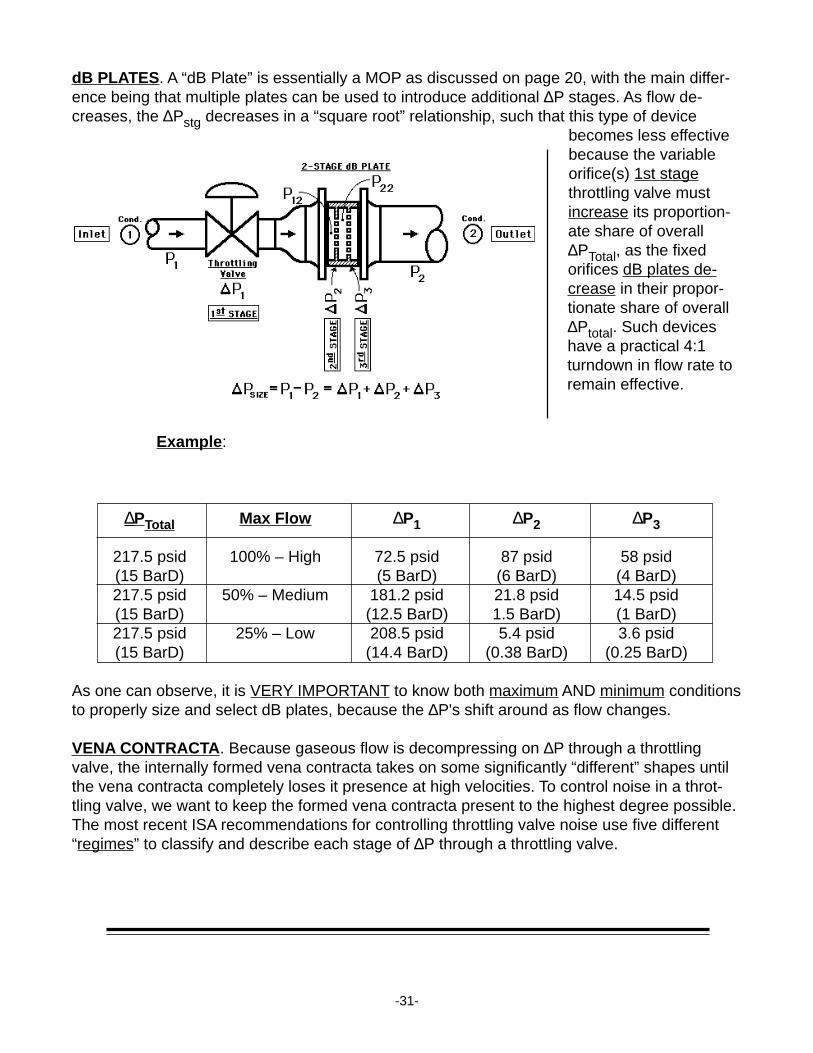
dB PLA TES. A “dB Plate” is essentially a MOP as discussed on page 20, with the main differ-ence being that multiple plates can be used to introduce additional ∆P stages. As flow de-creases, the ∆Pstg decreases in a “square root” relationship, such that this type of device
becomes less effectivebecause the variableorifice(s) 1st stagethrottling valve mustincrease its proportion-ate share of overall∆PTotal, as the fixedorifices dB plates de-crease in their propor-tionate share of overall∆Ptotal. Such deviceshave a practical 4:1turndown in flow rate toremain effective.
Example :
∆PTotal Max Flow ∆P1 ∆P2 ∆P3
217.5 psid 100% – High 72.5 psid 87 psid 58 psid(15 BarD) (5 BarD) (6 BarD) (4 BarD)217.5 psid 50% – Medium 181.2 psid 21.8 psid 14.5 psid(15 BarD) (12.5 BarD) 1.5 BarD) (1 BarD)217.5 psid 25% – Low 208.5 psid 5.4 psid 3.6 psid(15 BarD) (14.4 BarD) (0.38 BarD) (0.25 BarD)
As one can observe, it is VERY IMPORTANT to know both maximum AND minimum conditionsto properly size and select dB plates, because the ∆P's shift around as flow changes.
VENA CONTRACTA. Because gaseous flow is decompressing on ∆P through a throttlingvalve, the internally formed vena contracta takes on some significantly “different” shapes untilthe vena contracta completely loses it presence at high velocities. To control noise in a throt-tling valve, we want to keep the formed vena contracta present to the highest degree possible.The most recent ISA recommendations for controlling throttling valve noise use five different“regimes” to classify and describe each stage of ∆P through a throttling valve.
-32-
NOISE AND REGIMESNOISE AND REGIMES
There are several contributors when a high noise level is generated in a throttling valve. Themost obvious root causes are:
• High flow rate.• High pressure drop.• Low outlet pressure.• Basic valve type.
Any one of the above can be sufficient to generate excessive noise alone. When two or moreare together, one can expect up front that a noise level may be high (dBA > 85) or low(dBA < 85).
The following “rules-of-thumb” can be used as a tip-off to expect a noisy “throttling” applicationwhen the flow required is at Cv > 20:
• High Flow Rate. When the inlet pipe is 3" or 4" size, the flow carried is sufficiently highto probably cause high noise level with one other of the causes present also. A 6" inletpipe alone can carry sufficient flow to cause high noise primarily due to the mass flowrate alone.
High flow rates tend to generate broader frequency bands, including lower noisefrequency levels which are difficult for the pipe wall to “absorb” (i.e. “alternate”).
If the Cv Required is greater than Cv = 50, start expecting high noise level. If the CvRequired is greater than Cv = 100, the noise level will more than likely be high.
• High Pressure Drop. If the ∆PChoked is just reached and the flow is barely choked,noise level will likely be high. If the ∆PActual is greater than ∆PChoked by 15% orgreater, the noise level will likely be high.
An approximation of ∆PChoked can be as follows:
∆PChoked ≈ P1(absolute)/2.
High pressure drops tend to generate higher noise frequency levels.
• Low Outlet Pressure. When the outlet pressure is P2 < 25 psig (1.7 Barg), the outletdensity is relatively low, increasing the possibility of a high velocity, which in turn willgenerate high noise levels. This consideration alone will almost always cause a highnoise level to be developed if the ∆PChoked > 65 psid (4.5 Bard).
Low outlet pressures tend to generate lower noise frequency levels.
-33-
• A better indicator of expected noise is a combination of pressure drop and outlet pres-sure as follows:
When the PRatio exceeds 2.3 – 2.7 and there is Cv > 20, noise levels will likely behigh (dBA > 85) without the use of noise attenuating trim.
• Basic Valve Type. Different valve types with their different internal flow passage geom-etries will affect the noise levels generated. In general, the FL factors below can beused as a guide.
VALVE TYPE FL FACTOR RELATIVE NOISE LEVEL *
Globe 0.9 lowestEccentric plug - FTO 0.85Eccentric plug - FTC 0.68
Butterfly 0.65Ball 0.45 highest
* For same flow conditions.
Again in general, globe or FTO eccentric plug (rotary globe) valves are less noisythan a butterfly or ball valve.
REGIMES.
The new terminology concerning “Noise Regimes” definitions are as follows:
Regime I – Flow is subsonic and the P2 outlet pressure exhibits a high recovery (recom-pression) level; i.e. well formed, classical vena contracta. No “shock cells” formed.
High noise levels would not be expected, except at higher flow rates.
Pre
ssur
e
Time / Distance
P1
P2
Pressure Recovery Zone
Pvc
(EQ #16Repeated)
P1 = Pressure RatioP2 Abs)
-34-
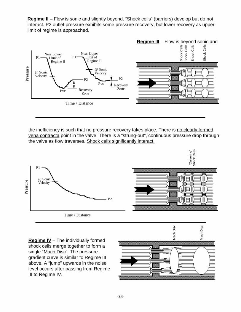
Regime II – Flow is sonic and slightly beyond. “Shock cells” (barriers) develop but do notinteract. P2 outlet pressure exhibits some pressure recovery, but lower recovery as upperlimit of regime is approached.
Regime III – Flow is beyond sonic and
Pre
ssur
e
Time / Distance
P1
P2
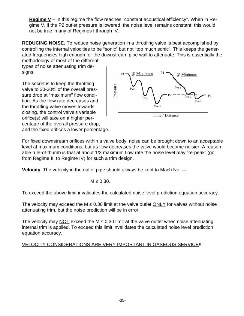
@ SonicVelocity
the inefficiency is such that no pressure recovery takes place. There is no clearly formedvena contracta point in the valve. There is a “strung-out”, continuous pressure drop throughthe valve as flow traverses. Shock cells significantly interact.
Regime IV – The individually formedshock cells merge together to form asingle “Mach Disc”. The pressuregradient curve is similar to Regime IIIabove. A “jump” upwards in the noiselevel occurs after passing from RegimeIII to Regime IV.
@ SonicVelocity
Pre
ssur
e
Time / Distance
P1Near Lower Limit of Regime II
Near Upper Limit of Regime II
P1
@ SonicVelocity
P2Pvc Recovery
ZoneRecoveryZone
Pvc
P2
Mac
h D
isc
Mac
h D
isc
“Qui
verin
g”S
hock
Cel
ls
Sho
ck C
ells
Sho
ck C
ells
Sho
ck C
ells
Sho
ck C
ells
-35-
Regime V – In this regime the flow reaches “constant acoustical efficiency”. When in Re-gime V, if the P2 outlet pressure is lowered, the noise level remains constant; this wouldnot be true in any of Regimes I through IV.
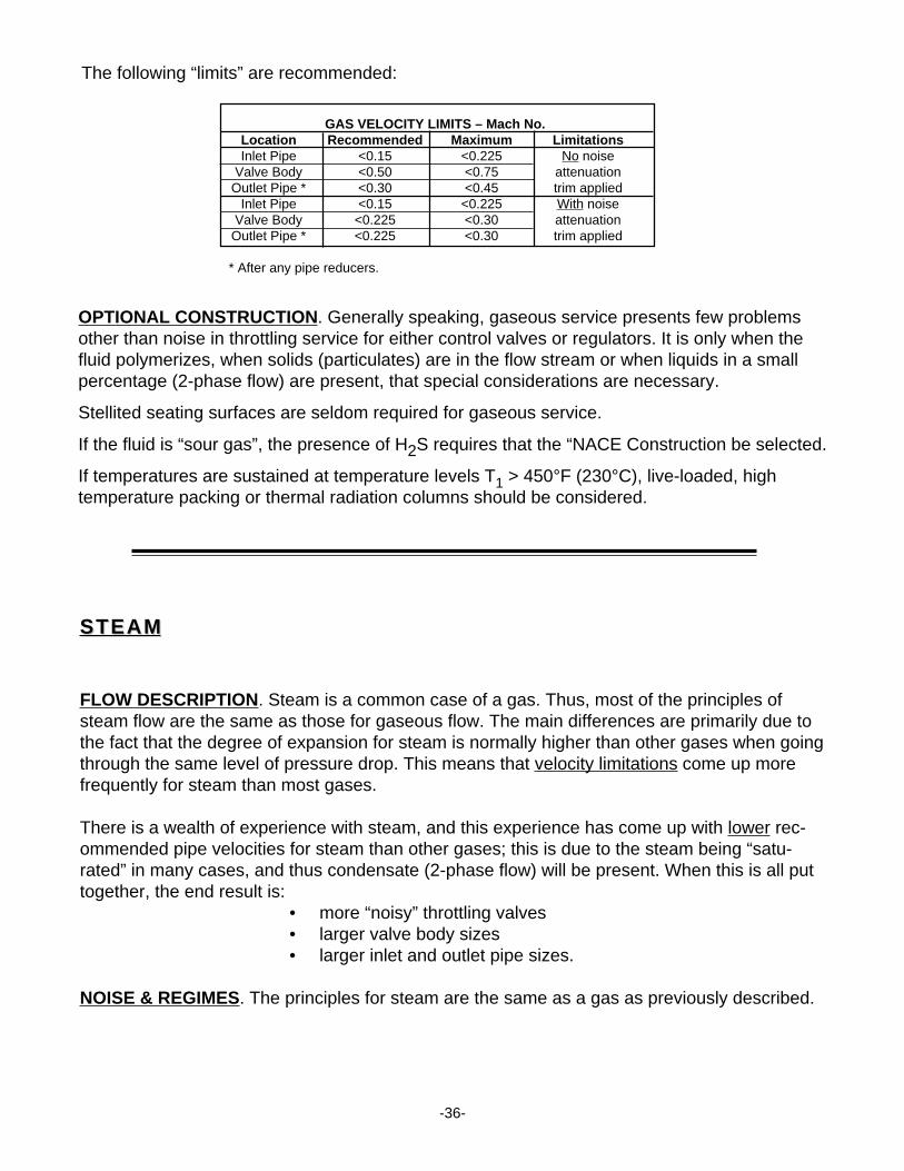
REDUCING NOISE. To reduce noise generation in a throttling valve is best accomplished bycontrolling the internal velocities to be “sonic” but not “too much sonic”. This keeps the gener-ated frequencies high enough for the downstream pipe wall to attenuate. This is essentially themethodology of most of the differenttypes of noise attenuating trim de-signs.
The secret is to keep the throttlingvalve to 20-30% of the overall pres-sure drop at “maximum” flow condi-tion. As the flow rate decreases andthe throttling valve moves towardsclosing, the control valve's variableorifice(s) will take on a higher per-centage of the overall pressure drop,and the fixed orifices a lower percentage.
For fixed downstream orifices within a valve body, noise can be brought down to an acceptablelevel at maximum conditions, but as flow decreases the valve would become noisier. A reason-able rule-of-thumb is that at about 1/3 maximum flow rate the noise level may “re-peak” (gofrom Regime III to Regime IV) for such a trim design.
Velocity . The velocity in the outlet pipe should always be kept to Mach No. —
M ≤ 0.30.
To exceed the above limit invalidates the calculated noise level prediction equation accuracy.
The velocity may exceed the M ≤ 0.30 limit at the valve outlet ONLY for valves without noiseattenuating trim, but the noise prediction will be in error.
The velocity may NOT exceed the M ≤ 0.30 limit at the valve outlet when noise attenuatinginternal trim is applied. To exceed this limit invalidates the calculated noise level predictionequation accuracy.
VELOCITY CONSIDERATIONS ARE VERY IMPORTANT IN GASEOUS SERVICE!!
Pre
ssur
eTime / Distance
P1
P2
P1
Pvc-1
Pvc-2
Pvc-3
P2
Pvc-1
Pvc-2
Pvc-3
@ _Maximum @ _Minimum
-36-
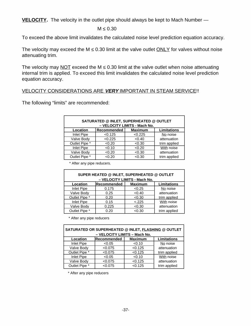
GAS VELOCITY LIMITS – Mach No.Location Recommended Maximum LimitationsInlet Pipe <0.15 <0.225 No noise
Valve Body <0.50 <0.75 attenuationOutlet Pipe * <0.30 <0.45 trim applied
Inlet Pipe <0.15 <0.225 With noiseValve Body <0.225 <0.30 attenuation
Outlet Pipe * <0.225 <0.30 trim applied
* After any pipe reducers.
The following “limits” are recommended:
OPTIONAL CONSTRUCTION . Generally speaking, gaseous service presents few problemsother than noise in throttling service for either control valves or regulators. It is only when thefluid polymerizes, when solids (particulates) are in the flow stream or when liquids in a smallpercentage (2-phase flow) are present, that special considerations are necessary.
Stellited seating surfaces are seldom required for gaseous service.
If the fluid is “sour gas”, the presence of H2S requires that the “NACE Construction be selected.
If temperatures are sustained at temperature levels T1 > 450°F (230°C), live-loaded, hightemperature packing or thermal radiation columns should be considered.
STEAMSTEAM
FLOW DESCRIPTION. Steam is a common case of a gas. Thus, most of the principles ofsteam flow are the same as those for gaseous flow. The main differences are primarily due tothe fact that the degree of expansion for steam is normally higher than other gases when goingthrough the same level of pressure drop. This means that velocity limitations come up morefrequently for steam than most gases.
There is a wealth of experience with steam, and this experience has come up with lower rec-ommended pipe velocities for steam than other gases; this is due to the steam being “satu-rated” in many cases, and thus condensate (2-phase flow) will be present. When this is all puttogether, the end result is:
• more “noisy” throttling valves• larger valve body sizes• larger inlet and outlet pipe sizes.
NOISE & REGIMES. The principles for steam are the same as a gas as previously described.
-37-
SATURATED @ INLET, SUPERHEATED @ OUTLET– VELOCITY LIMITS - Mach No.
Location Recommended Maximum LimitationsInlet Pipe <0.125 <0.225 No noise
Valve Body <0.225 <0.40 attenuationOutlet Pipe * <0.20 <0.30 trim applied
Inlet Pipe <0.10 <0.20 With noiseValve Body <0.20 <0.30 attenuation
Outlet Pipe * <0.20 <0.30 trim applied
* After any pipe reducers.
VELOCITY. The velocity in the outlet pipe should always be kept to Mach Number —
M ≤ 0.30
To exceed the above limit invalidates the calculated noise level prediction equation accuracy.
The velocity may exceed the M ≤ 0.30 limit at the valve outlet ONLY for valves without noiseattenuating trim.
The velocity may NOT exceed the M ≤ 0.30 limit at the valve outlet when noise attenuatinginternal trim is applied. To exceed this limit invalidates the calculated noise level predictionequation accuracy.
VELOCITY CONSIDERATIONS ARE VERY IMPORTANT IN STEAM SERVICE!!
The following “limits” are recommended:
SUPER HEATED @ INLET, SUPERHEATED @ OUTLET– VELOCITY LIMITS - Mach No.
Location Recommended Maximum LimitationsInlet Pipe 0.175 <0.25 No noise
Valve Body 0.25 <0.40 attenuationOutlet Pipe * 0.20 <0.30 trim applied
Inlet Pipe 0.15 <.225 With noiseValve Body 0.225 <0.30 attenuation
Outlet Pipe * 0.20 <0.30 trim applied
* After any pipe reducers
SATURATED OR SUPERHEATED @ INLET, FLASHING @ OUTLET– VELOCITY LIMITS – Mach No.
Location Recommended Maximum LimitationsInlet Pipe <0.05 <0.10 No noise
Valve Body <0.075 <0.125 attenuationOutlet Pipe * <0.075 <0.125 trim applied
Inlet Pipe <0.05 <0.10 With noiseValve Body <0.075 <0.125 attenuation
Outlet Pipe * <0.075 <0.125 trim applied
* After any pipe reducers
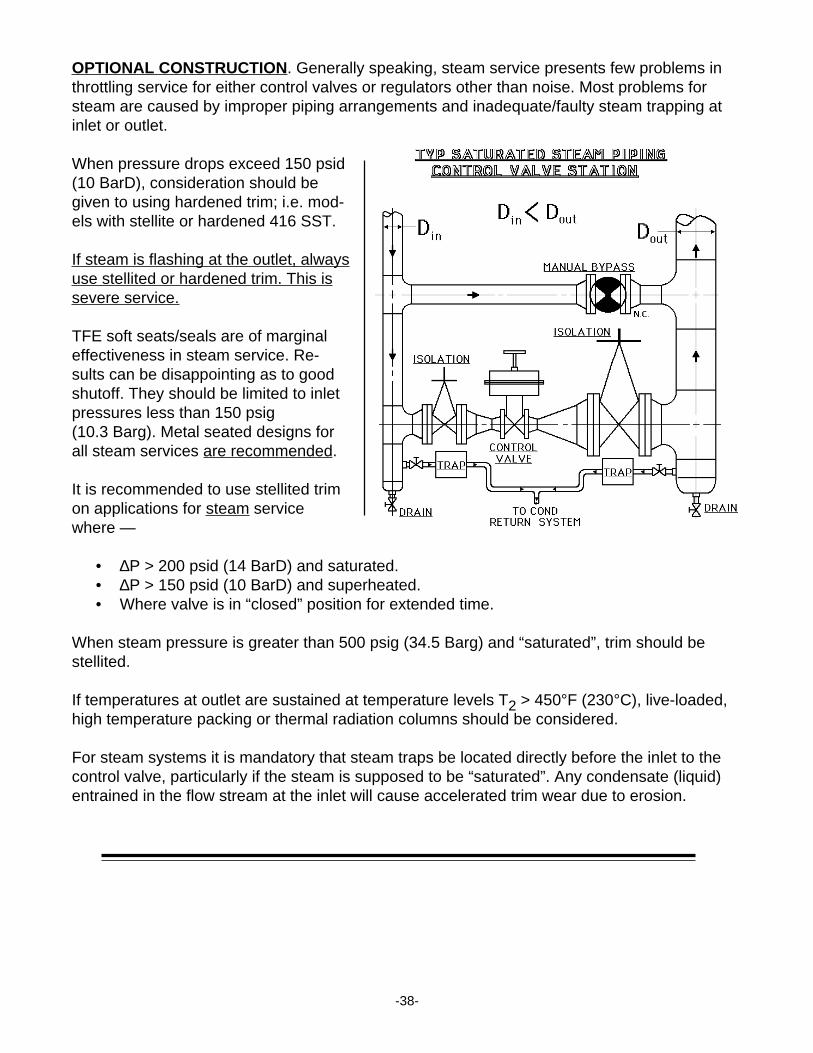
-38-
OPTIONAL CONSTRUCTION . Generally speaking, steam service presents few problems inthrottling service for either control valves or regulators other than noise. Most problems forsteam are caused by improper piping arrangements and inadequate/faulty steam trapping atinlet or outlet.
When pressure drops exceed 150 psid(10 BarD), consideration should begiven to using hardened trim; i.e. mod-els with stellite or hardened 416 SST.
If steam is flashing at the outlet, alwaysuse stellited or hardened trim. This issevere service.
TFE soft seats/seals are of marginaleffectiveness in steam service. Re-sults can be disappointing as to goodshutoff. They should be limited to inletpressures less than 150 psig(10.3 Barg). Metal seated designs forall steam services are recommended.
It is recommended to use stellited trimon applications for steam servicewhere —
• ∆P > 200 psid (14 BarD) and saturated.• ∆P > 150 psid (10 BarD) and superheated.• Where valve is in “closed” position for extended time.
When steam pressure is greater than 500 psig (34.5 Barg) and “saturated”, trim should bestellited.
If temperatures at outlet are sustained at temperature levels T2 > 450°F (230°C), live-loaded,high temperature packing or thermal radiation columns should be considered.
For steam systems it is mandatory that steam traps be located directly before the inlet to thecontrol valve, particularly if the steam is supposed to be “saturated”. Any condensate (liquid)entrained in the flow stream at the inlet will cause accelerated trim wear due to erosion.
-39-
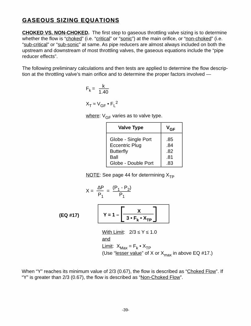
GASEOUS SIZING EQUATIONSGASEOUS SIZING EQUATIONS
CHOKED VS. NON-CHOKED. The first step to gaseous throttling valve sizing is to determinewhether the flow is “choked” (i.e. “critical” or “sonic”) at the main orifice, or “non-choked” (i.e.“sub-critical” or “sub-sonic” at same. As pipe reducers are almost always included on both theupstream and downstream of most throttling valves, the gaseous equations include the “pipereducer effects”.
The following preliminary calculations and then tests are applied to determine the flow descrip-tion at the throttling valve’s main orifice and to determine the proper factors involved —
Fk =k
1.40
XT ≈ VGF • FL2
where: VGF varies as to valve type.
Valve Type V GF
Globe - Single Port .85Eccentric Plug .84Butterfly .82Ball .81Globe - Double Port .83
NOTE: See page 44 for determining XTP
X =∆P
=(P1 - P2)
P1 P1
When “Y” reaches its minimum value of 2/3 (0.67), the flow is described as “Choked Flow”. If“Y” is greater than 2/3 (0.67), the flow is described as “Non-Choked Flow”.
(EQ #17) Y = 1 –X
3 • Fk • XTP
With Limit: 2/3 ≤ Y ≤ 1.0andLimit: XMax = Fk • XTP(Use “lesser value” of X or Xmax in above EQ #17.)
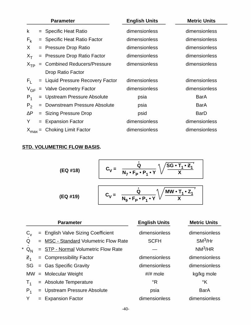
-40-
Parameter English Units Metric Units
k = Specific Heat Ratio dimensionless dimensionless
Fk = Specific Heat Ratio Factor dimensionless dimensionless
X = Pressure Drop Ratio dimensionless dimensionless
XT = Pressure Drop Ratio Factor dimensionless dimensionless
XTP = Combined Reducers/Pressure dimensionless dimensionless
Drop Ratio Factor
FL = Liquid Pressure Recovery Factor dimensionless dimensionless
VGF = Valve Geometry Factor dimensionless dimensionless
P1 = Upstream Pressure Absolute psia BarA
P2 = Downstream Pressure Absolute psia BarA
∆P = Sizing Pressure Drop psid BarD
Y = Expansion Factor dimensionless dimensionless
Xmax = Choking Limit Factor dimensionless dimensionless
STD. VOLUMETRIC FLOW BASIS.
(EQ #18) CV =Q SG • T1 • Z1
N7 • FP • P1 • Y X
.
(EQ #19) CV =Q MW • T1 • Z1
N9 • FP • P1 • Y X
.
Parameter English Units Metric Units
Cv = English Valve Sizing Coefficient dimensionless dimensionless
Q = MSC - Standard Volumetric Flow Rate SCFH SM3/Hr
* QN = STP - Normal Volumetric Flow Rate — NM3/HR
Z1 = Compressibility Factor dimensionless dimensionless
SG = Gas Specific Gravity dimensionless dimensionless
MW = Molecular Weight #/# mole kg/kg mole
T1 = Absolute Temperature °R °K
P1 = Upstream Pressure Absolute psia BarA
Y = Expansion Factor dimensionless dimensionless
.
.
-41-
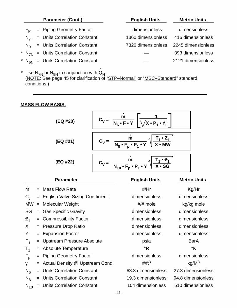
Parameter (Cont.) English Units Metric Units
FP = Piping Geometry Factor dimensionless dimensionless
N7 = Units Correlation Constant 1360 dimensionless 416 dimensionless
N9 = Units Correlation Constant 7320 dimensionless 2245 dimensionless
* N7N = Units Correlation Constant — 393 dimensionless
* N9N = Units Correlation Constant — 2121 dimensionless
* Use N7N or N9N in conjunction with QN.(NOTE: See page 45 for clarification of “STP–Normal” or “MSC–Standard” standardconditions.)
.
MASS FLOW BASIS.
(EQ #20) CV =m 1
N6 • F • Y X • P1 • γ1
.
(EQ #21) CV =m T1 • Z1
N8 • Fp • P1 • Y X • MW
.
(EQ #22) CV =m T1 • Z1
N10 • Fp • P1 • Y X • SG
.
Parameter English Units Metric Units
m = Mass Flow Rate #/Hr Kg/Hr
Cv = English Valve Sizing Coefficient dimensionless dimensionless
MW = Molecular Weight #/# mole kg/kg mole
SG = Gas Specific Gravity dimensionless dimensionless
Z1 = Compressibility Factor dimensionless dimensionless
X = Pressure Drop Ratio dimensionless dimensionless
Y = Expansion Factor dimensionless dimensionless
P1 = Upstream Pressure Absolute psia BarA
T1 = Absolute Temperature °R °KFp = Piping Geometry Factor dimensionless dimensionless
γ = Actual Density @ Upstream Cond. #/ft3 kg/M3
N6 = Units Correlation Constant 63.3 dimensionless 27.3 dimensionless
N8 = Units Correlation Constant 19.3 dimensionless 94.8 dimensionless
N10 = Units Correlation Constant 104 dimensionless 510 dimensionless
.
-42-
STEAM. As steam is a vapor/gas that does not exist as a fluid within piping systems at stan-dard conditions of pressure and temperature, Equation #20 is utilized using actual density —γActual and mass flow basis. As this equation is based on “actual non-volumetric” conditions,
there is no Compressibility Factor – Z1 required to correct for deviation from the ideal gas laws.Should Equations #21 or #22 be utilized, these are based on the ideal gas laws, so Compress-ibility Factor – Z1 is required as an input.
MISCELLANEOUSMISCELLANEOUS — —PIPE REDUCERS CORRECTION FACTORSPIPE REDUCERS CORRECTION FACTORS
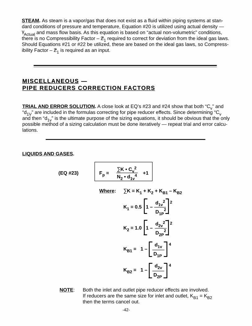
TRIAL AND ERROR SOLUTION. A close look at EQ’s #23 and #24 show that both “Cv” and“d1V” are included in the formulas correcting for pipe reducer effects. Since determining “Cvand then “d1v” is the ultimate purpose of the sizing equations, it should be obvious that the onlypossible method of a sizing calculation must be done iteratively — repeat trial and error calcu-lations.
LIQUIDS AND GASES.
NOTE: Both the inlet and outlet pipe reducer effects are involved.If reducers are the same size for inlet and outlet, KB1 = KB2then the terms cancel out.
Fp =∑K • Cv
2+1
N2 • d1v4
Where: ∑K = K1 + K2 + KB1 – KB2
K1 = 0.5 1 – d1v
2 2
D1P2
K2 = 1.0 1 – d2v
2 2
D2P2
KB1 = 1 – d1v
4
D1P
KB2 = 1 – d2v
4
D2P
(EQ #23)
-43-
Parameter English Units Metric Units
FP = Piping Geometry Factor dimensionless dimensionless
∑K = Combined Head Loss Coefficient dimensionless dimensionless
Cv = English Valve Sizing Coefficient dimensionless dimensionless
N2 = Units Correlation Constant 890 dimensionless 0.00214 dimensionless
d1V = Valve Inlet Body Size in. mm
d2V = Valve Outlet Body Size in. mm
D1P = Inlet Pipe Size (before reducer) in. mm
D2P = Outlet Pipe Size (after reducer) in. mm
K1 = Inlet Resistance Coefficient dimensionless dimensionless
K2 = Outlet Resistance Coefficient dimensionless dimensionless
K1B = Inlet Bernoulli Coefficient dimensionless dimensionless
K2B = Outlet Bernoulli Coefficient dimensionless dimensionless
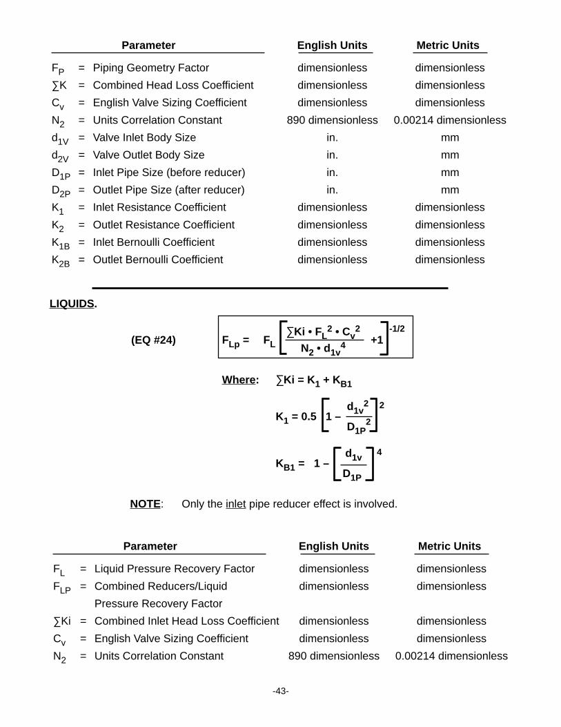
NOTE: Only the inlet pipe reducer effect is involved.
LIQUIDS.
Parameter English Units Metric Units
FL = Liquid Pressure Recovery Factor dimensionless dimensionless
FLP = Combined Reducers/Liquid dimensionless dimensionless
Pressure Recovery Factor
∑Ki = Combined Inlet Head Loss Coefficient dimensionless dimensionless
Cv = English Valve Sizing Coefficient dimensionless dimensionless
N2 = Units Correlation Constant 890 dimensionless 0.00214 dimensionless
FLp = FL∑Ki • FL
2 • Cv2
+1 -1/2
N2 • d1v4
Where: ∑Ki = K 1 + KB1
K1 = 0.5 1 – d1v
2 2
D1P2
KB1 = 1 – d1v
4
D1P
(EQ #24)
-44-
Parameter (Cont.) English Units Metric Units
d1V = Valve Inlet Body Size in. mm
D1P = Inlet Pipe Size (before reducer) in. mm
K1 = Inlet Resistance Coefficient dimensionless dimensionless
KB1 = Inlet Bernoulli Coefficient dimensionless dimensionless
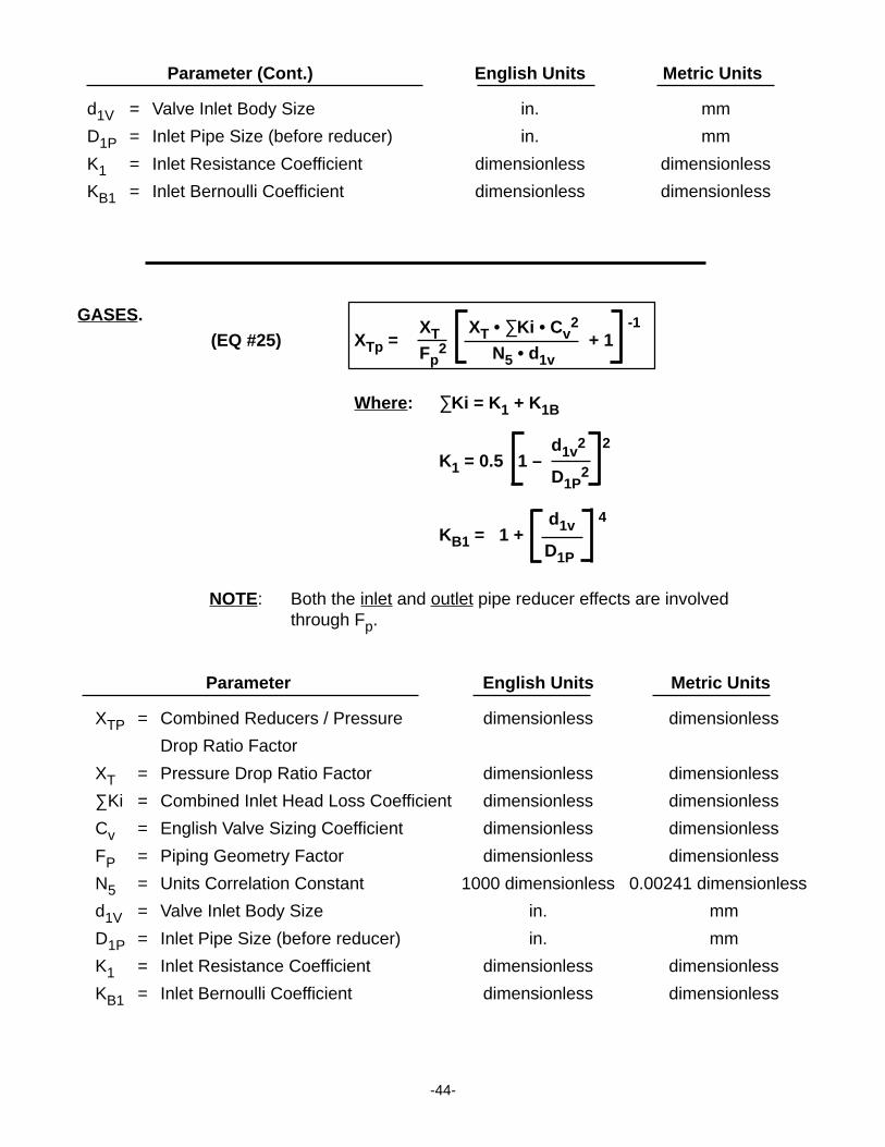
NOTE: Both the inlet and outlet pipe reducer effects are involvedthrough Fp.
Parameter English Units Metric Units
XTP = Combined Reducers / Pressure dimensionless dimensionless
Drop Ratio Factor
XT = Pressure Drop Ratio Factor dimensionless dimensionless
∑Ki = Combined Inlet Head Loss Coefficient dimensionless dimensionless
Cv = English Valve Sizing Coefficient dimensionless dimensionless
FP = Piping Geometry Factor dimensionless dimensionless
N5 = Units Correlation Constant 1000 dimensionless 0.00241 dimensionless
d1V = Valve Inlet Body Size in. mm
D1P = Inlet Pipe Size (before reducer) in. mm
K1 = Inlet Resistance Coefficient dimensionless dimensionless
KB1 = Inlet Bernoulli Coefficient dimensionless dimensionless
GASES.(EQ #25) XTp =
XT XT • ∑Ki • Cv2
+ 1-1
Fp2 N5 • d1v
Where: ∑Ki = K 1 + K1B
K1 = 0.5 1 – d1v
2 2
D1P2
KB1 = 1 + d1v
4
D1P
-45-
STANDARD CONDITIONS FOR GASES
_ENGLISH
Std. Temp. = 60°F
Std. Pressure = 14.7 psia
_METRIC
“MSC” – Metr ic Std. Conditions
Std. Temp. = 15°C
Std. Pressure = 1 Atm
“STP” – Std. Temp. & Pressure
or
“N” = Normal
Std. Temp = 0°C
Std. Pressure = 1 Atm
_“_Normal_” Metric Volume “_Standard_” Metric Volume
NM /Hr3 SM /Hr M /Hr3 3
S lit/min lit/minN lit/min
If the flow rate does not indicate as “N” or an “S”,assume that it means “standard” metr ic volume.
IDEAL GAS vs. REALITY—
Use of the ideal gas law is extensive in the process industry with a correction factor to adjust for the “ ideal vs. real” conditions. This correction factor is known as —
_ Z - the “compressibility factor”
Combined IdealGas Law
Combined RealGas Law
P V P V1 1 2 2
T1 T2
=P1V1
T12
P2V2T2
xx1Z Z=
PV = nRT
PV = mRT
PV = ZnRT
PV = ZmRT
_SPECIFIC GRAVITY – DENSITY – MOLECULAR WEIGHT
ρ OR γ (rho or gamma are used as density terms)
ρ STD =_ MW V molar
SG gas = ρ fluid
ρ air
ENGLISH METRIC - STP
ρ air = .07622 #/ft = ρSTD
V molar = 379.8 ft /# mole
@ 60°F & 14.7 psia (1 ATM)
3
3
ρ air = 1.2924 kg/m = ρSTP
V molar = 22.40 m /kg - mole
@ 0°C & 1 ATM
3
3
SG = 13.120 x ρFluid
MW = 379.8 x ρSTD.
MW = 28.95 x SG STD.
SG = .7738 x ρFluid
MW = 22.40 x ρSTP.
MW = 28.95 x SGSTP.
METRIC - MSC
@ 15°C & 1 ATM
SG = .8180 x ρFluid
MW = 23.68 x ρMSC
MW = 28.95 x SG MSC
ρ air = 1.2225 kg /m = ρ MSC
V molar = 23.68 m /kg - mole
3
3
By the “_law of conservation of mass” we know that _m = _m , as a valve does not “store” any mass, and most processes experience “_steady-state, steady flow” conditions. A gaseous _mass flow rate represents an “_actual flow rate”.
When gaseous flow is expressed as a “_volumetric flow rate @ standard conditions” — SCFH, SCFM, NM /Hr, SM /Hr, etc., this flow rate is a “_fictious” flow rate that could not occur if a pressure drop takes place. Standard volumetric flow rates are used for ease of mathematical manipulation and application to the “_combined ideal gas law” and the “_basic equation of state”.
Q above _must be equal to Q , for the above. It is a convenient way to calculate with a basis of Q = Q . Thus, both the Q and Q are “_fictious”. Any “_actual” calculation — such as a velocity calculation — would have to be converted to Q or Q to do correctly. To calculate a velocity directly from SCFH or NM /Hr would be a waste of time as it would be meaningless.
inout
3 3
1 2
in
_outin
out
in actual out actual3
..
..
. .
. .
1 2
∆P
1 2
∆P
Q = 15,000 SCFH Q = ??
Q = 430 SM /hr Q = ??2M1M3
1E
.
.
2E
.
.
m = 5000 #/hr m = 5000 #/hr
m = 2500 kg/hr m = 2500 kg/hr
1E 2E. .
1M 2M. .
VOLUMETRIC FLOW STD CONDITIONSvs.
MASS FLOW—GAS
-46-
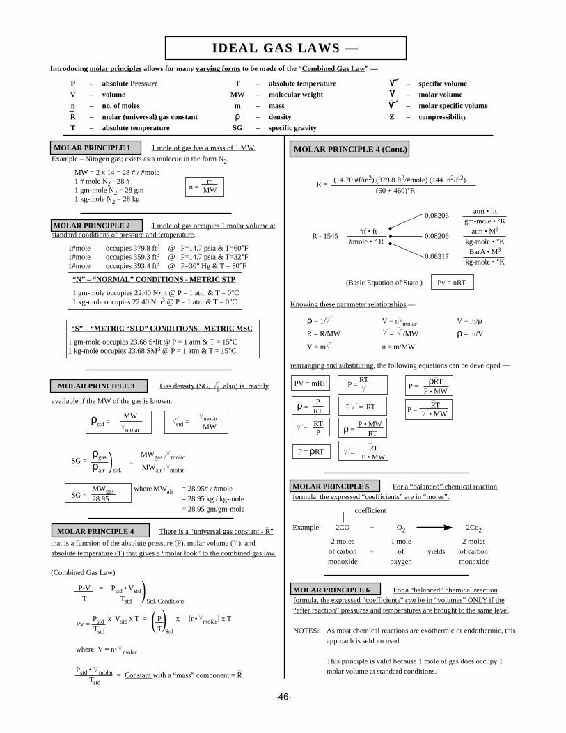
Knowing these parameter relationships —
ρ = 1/ V = n molar V = m/ρ
R = R/MW = /MW ρ = m/V
V = m n = m/MW
rearranging and substituting, the following equations can be developed —
R =(14.70 #f/in2) (379.8 ft3/#mole) (144 in2/ft2)
(60 + 460)°R
0.08206atm • lit
gm-mole • °K
R - 1545#f • ft
0.08206atm • M3
#mole • ° R kg-mole • °K
0.08317BarA • M3
kg-mole • °K
ρstd =
MW std =
molar
molar MW
IDEAL GAS LAWS —IDEAL GAS LAWS —
SG =ρgas
=
MWgas / molar
ρair std. MWair / molar
SG =MWgas where MWair = 28.95# / #mole28.95 = 28.95 kg / kg-mole
= 28.95 gm/gm-mole
)
MOLAR PRINCIPLE 4 There is a “universal gas constant - R”
that is a function of the absolute pressure (P), molar volume ( ), andabsolute temperature (T) that gives a “molar look” to the combined gas law.
(Combined Gas Law)
P•V = Pstd • VstdT Tstd Std. Conditions
Pv =Pstd x Vstd x T = P x [n• molar] x TTstd T Std
where, V = n• molar
Pstd • molar = Constant with a “mass” component = RTstd
)))
(Basic Equation of State ) Pv = nRT
MOLAR PRINCIPLE 4 (Cont.)
P = ρRT
PV = mRT
ρ =P
RT
MOLAR PRINCIPLE 5 For a “balanced” chemical reactionformula, the expressed “coefficients” are in “moles”.
Example – 2CO + O2 2Co2
2 moles 1 mole 2 molesof carbon + of yields of carbonmonoxide oxygen monoxide
coefficient
MOLAR PRINCIPLE 6 For a “balanced” chemical reactionformula, the expressed “coefficients” can be in “volumes” ONLY if the“after reaction” pressures and temperatures are brought to the same level.
NOTES: As most chemical reactions are exothermic or endothermic, thisapproach is seldom used.
This principle is valid because 1 mole of gas does occupy 1molar volume at standard conditions.
P =ρRT
P • MWP =
RT
P = RT
ρ = P • MW
RT=
RTP
=RT
P • MW
P = RT
• MW
Introducing molar principles allows for many varying forms to be made of the “Combined Gas Law” —
P – absolute Pressure T – absolute temperature – specific volume
V – volume MW – molecular weight – molar volume
n – no. of moles m – mass – molar specific volume
R – molar (universal) gas constant ρ – density Z – compressibility
T – absolute temperature SG – specific gravity
MOLAR PRINCIPLE 1 1 mole of gas has a mass of 1 MW.
Example – Nitogen gas; exists as a molecue in the form N2.
MW = 2 x 14 = 28 # / #mole1 # mole N2 - 28 #
n =m
1 gm-mole N2 = 28 gm MW1 kg-mole N2 = 28 kg
MOLAR PRINCIPLE 2 1 mole of gas occupies 1 molar volume atstandard conditions of pressure and temperature.
1#mole occupies 379.8 ft3 @ P=14.7 psia & T=60°F1#mole occupies 359.3 ft3 @ P=14.7 psia & T=32°F1#mole occupies 393.4 ft3 @ P=30" Hg & T = 80°F
“N” – “NORMAL” CONDITIONS - METRIC STP
1 gm-mole occupies 22.40 N•lit @ P = 1 atm & T = 0°C1 kg-mole occupies 22.40 Nm3 @ P = 1 atm & T = 0°C
“S” – “METRIC “STD” CONDITIONS - METRIC MSC
1 gm-mole occupies 23.68 S•lit @ P = 1 atm & T = 15°C1 kg-mole occupies 23.68 SM3 @ P = 1 atm & T = 15°C
MOLAR PRINCIPLE 3 Gas density (SG, also) is readily
available if the MW of the gas is known.
g
-47-
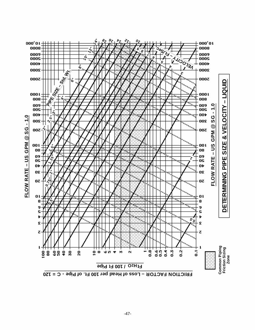
PIPE
SIZ
E –
Std.
Wt.
2"
3"
4"
6"
8"10
"12
"14
"
0.5"
1"
3
45
67
89
141618
1
2
VELOCITY – Ft./Sec.
0.5
DE
TER
MIN
ING
PIP
E S
IZE
& V
ELO
CIT
Y –
LIQ
UID
12
1.2
5"
1.5"
2.5"
Com
mon
Pip
ing
Fric
tion
Siz
ing
Zon
e
0.75
"
FLO
W R
AT
E –
US
GP
M @
SG
- 1
.0
FLO
W R
AT
E –
US
GP
M @
SG
- 1
.0
FRICTION FACTOR – Loss of Head per 100 Ft. of Pipe - C = 120
Ft / 100 Ft Pipe H2O
10
-48-
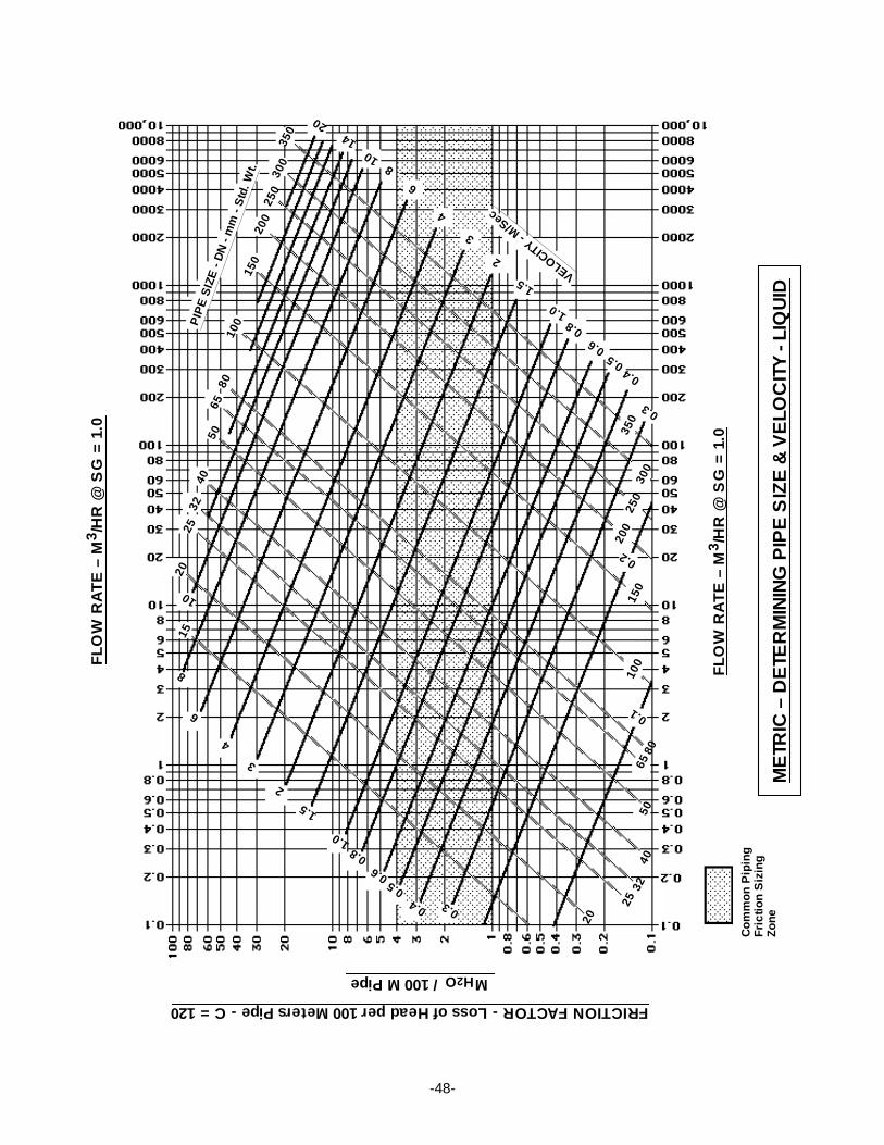
0.1
0.2
0.30.40.5
0.60.8
1.0
1.5
2
3
4
6
8
10
1520
2532
4050
6580
100
150
200
250
300
350
0.3
0.40.5
0.60.8
1.0
1.5
2
3
6
810
4
1420
FLO
W R
AT
E –
M
/HR
@ S
G =
1.0
3
FLO
W R
AT
E –
M
/HR
@ S
G =
1.0
3
FRICTION FACTOR - Loss of Head per 100 Meters Pipe - C = 120
Com
mon
Pip
ing
Fric
tion
Siz
ing
Zon
e
PIP
E S
IZE
- D
N -
mm
- S
td. W
t.
VELOCITY - M/S
ec
ME
TRIC
– D
ETE
RM
ININ
G P
IPE
SIZ
E &
VE
LOC
ITY
- LI
QU
ID
20
2532
4050
6580
100
150
200
250
300
350
M / 100 M Pipe H2O
-49-
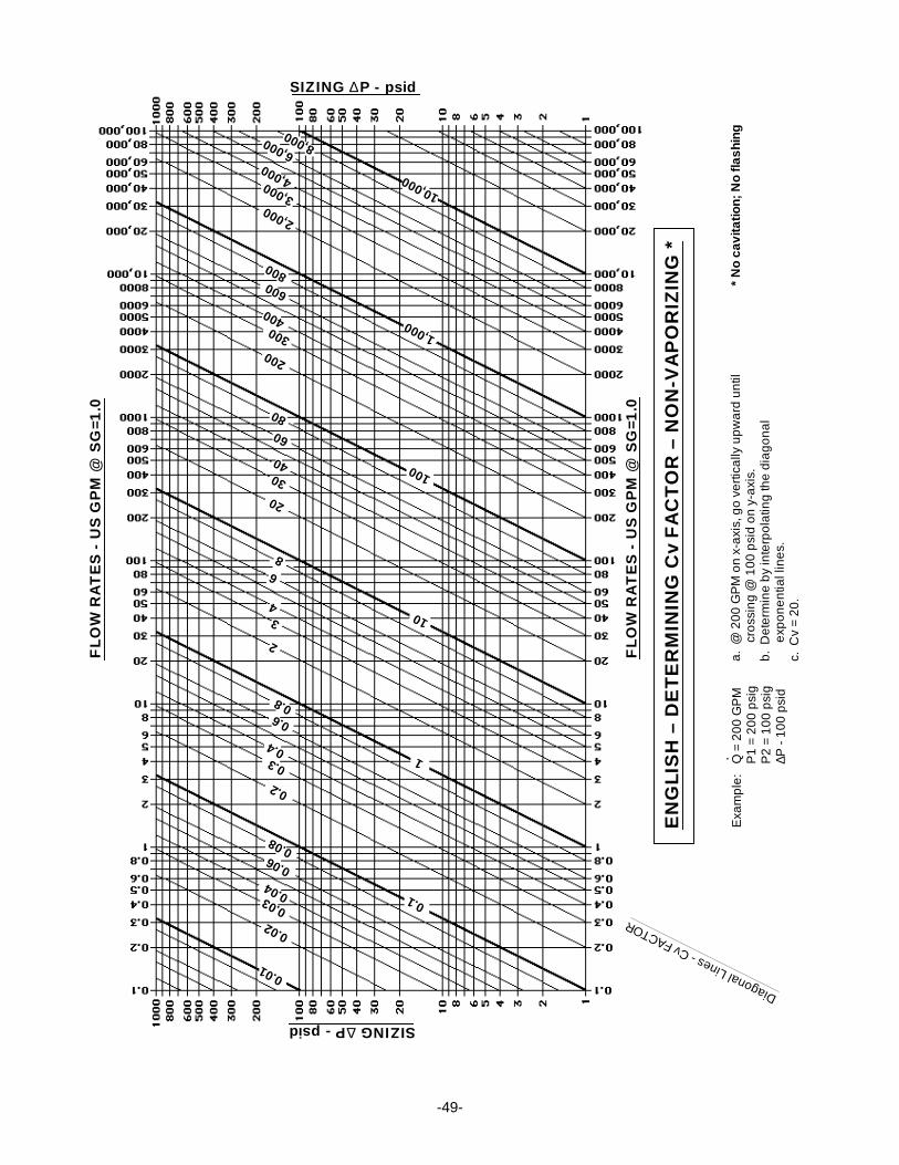
FLO
W R
AT
ES
- U
S G
PM
@ S
G=1
.0
Exa
mp
le:
a.
@ 2
00
GP
M o
n x
-axi
s, g
o v
ert
ica
lly u
pw
ard
un
til
cr
oss
ing
@ 1
00
psi
d o
n y
-axi
s.b
. D
ete
rmin
e b
y in
terp
ola
ting
the
dia
go
na
l
e
xpo
ne
ntia
l lin
es.
c. C
v =
20
.
* N
o ca
vita
tio
n; N
o fla
shin
g
EN
GLI
SH
– D
ET
ER
MIN
ING
Cv
FA
CT
OR
– N
ON
-VA
PO
RIZ
ING
*
0.01
0.1
1 Q =
20
0 G
PM
P1
= 2
00
psi
gP
2 =
10
0 p
sig
∆P -
10
0 p
sid
.
Diagonal Lines - Cv FACTOR
FLO
W R
AT
ES
- U
S G
PM
@ S
G=1
.0
SIZING ∆P - psid
SIZING ∆P - psid
2
4
6 8
10
100
1,000
10,000
0.2
0.4
0.60.8
20
40
6080
2,000
4,000
3,000
6,000 8,000
200300400
600800
30
3
0.3
0.020.03 0.04
0.060.08
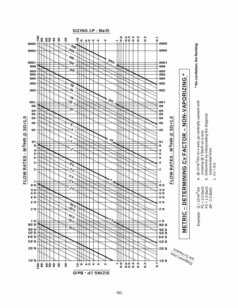
-50-
Exa
mp
le:
ME
TR
IC –
DE
TE
RM
ININ
G C
v F
AC
TO
R –
NO
N-V
AP
OR
IZIN
G *
SIZING ∆P - BarDSIZING ∆P - BarD
Diagonal Lines
are Cv Factors
* N
o ca
vita
tio
n; N
o fla
shin
gQ
= 1
0 M
/H
rP
1 =
3.0
Ba
rGP
2 =
1.0
Ba
rG∆P
- 2
.0 B
arD
.3
a.
@ 1
0 M
/H
r o
n x
-axi
s, g
o v
ert
ica
lly u
pw
ard
un
til
cr
oss
ing
@ 2
Ba
rD o
n y
-axi
s.b
. D
ete
rmin
e b
y in
terp
ola
ting
the
dia
go
na
l
e
xpo
ne
ntia
l lin
es.
c. C
v ≈
8.0
.3
0.04
0.1
1
6
8
10
100
1000
FLO
W R
AT
ES
- M
/H
R @
SG
=1.0
3 2
4F
LOW
RA
TE
S -
M /
HR
@ S
G=1
.03
0.06 0.08
0.2
0.30.4
0.60.8
3
20
3040
6080
200
300400
600800
0.02
0.03
-51-
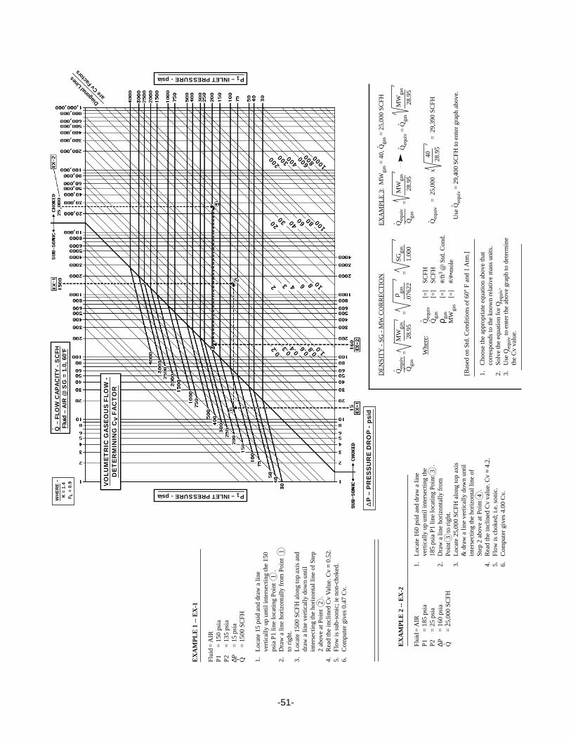
.
EX
AM
PLE
1 -
- E
X-1
Flu
id=
AIR
P1
= 1
50 p
sia
P2
= 1
35 p
sia
∆P=
15
psia
Q=
150
0 S
CF
H
1.Lo
cate
15
psid
and
dra
w a
line
vert
ical
ly u
p un
til in
ters
ectin
g th
e 15
0ps
ia P
1 lin
e lo
catin
g P
oint
1
.2.
Dra
w a
line
hor
izon
tally
from
Poi
nt
1to
rig
ht.
3.Lo
cate
150
0 S
CF
H a
long
top
axis
and
draw
a li
ne v
ertic
ally
dow
n un
tilin
ters
ectin
g th
e ho
rizon
tal l
ine
of S
tep
2 ab
ove
at P
oint
2
.4.
Rea
d th
e in
clin
ed C
v Va
lue.
Cv ≈ 0.
52.
5.F
low
is s
ub-s
onic
; ie
non-
chok
ed.
6.C
ompu
ter
give
s 0.
47 C
v.
.
EX
AM
PLE
3:
MW
gas =
40,
Qga
s = 2
5,00
0 S
CF
H
Qeq
uiv
=M
Wga
sQ
equi
v = Q
gas
MW
gas
Qga
s28
.95
28.9
5
Qeq
uiv
= 2
5,00
0 x
40=
29,
390
SC
FH
28.9
5
Use
Qeq
uiv =
29,
400
SC
FH
to e
nter
gra
ph a
bove
.
.
. ..
.
.
.
EX
AM
PLE
2 -
- E
X-2
Flu
id=
AIR
1.Lo
cate
160
psi
d an
d dr
aw a
line
P1
= 1
85 p
sia
vert
ical
ly u
p un
til in
ters
ectin
g th
eP
2=
25
psia
185
psia
P1
line
loca
ting
Poi
nt 3
.∆P
= 1
60 p
sia
2.D
raw
a li
ne h
oriz
onta
lly fr
omQ
= 2
5,00
0 S
CF
HP
oint
3 t
o rig
ht.
3.Lo
cate
25,
000
SC
FH
alo
ng to
p ax
is&
dra
w a
line
ver
tical
ly d
own
until
inte
rsec
ting
the
horiz
onta
l lin
e of
Ste
p 2
abov
e at
Poi
nt 4
.4.
Rea
d th
e in
clin
ed C
v va
lue.
Cv ≈ 4.
2.5.
Flo
w is
cho
ked;
i.e.
son
ic.
6.C
ompu
ter
give
s 4.
00 C
v.
.
DE
NS
ITY
- S
G -
MW
CO
RR
EC
TIO
N
Qeq
uiv
=M
Wga
s=
ρ gas
=S
Gga
s
Qga
s28
.95
.076
221.
000
Whe
re:
Q equ
iv[=
]S
CF
HQ
gas
[=]
SC
FH
ρ gas
[=]
#/ft
3 @
Std
. Con
d.M
Wga
s[=
]#/
#•m
ole
[Bas
ed o
n S
td. C
ondi
tions
of 6
0°
F a
nd 1
Atm
.]
1.C
hoos
e th
e ap
prop
riate
equ
atio
n ab
ove
that
corr
espo
nds
to th
e kn
own
rela
tive
mas
s un
its.
2.S
olve
the
equa
tion
for
Q equi
v.3.
Use
Qeq
uiv t
o en
ter
the
abov
e gr
aph
to d
eter
min
eth
e C
v va
lue.
. .
. .
..
0.2 0.3 0.4 0.6
0.8 1.0
32 4 6 108
20 30
40 60 80
1001000
800600400300
200
Diagon
al Lin
es
are C
v Fac
tors
vV
OLU
ME
TR
IC G
AS
EO
US
FLO
W -
DE
TE
RM
ININ
G C
F
AC
TO
R
WH
ER
E –
K =
1.4
F
= 0
.9L
Q –
FLO
W C
AP
AC
ITY
- S
CF
HF
luid
– A
IR @
SG
= 1
.0,
60°F
.
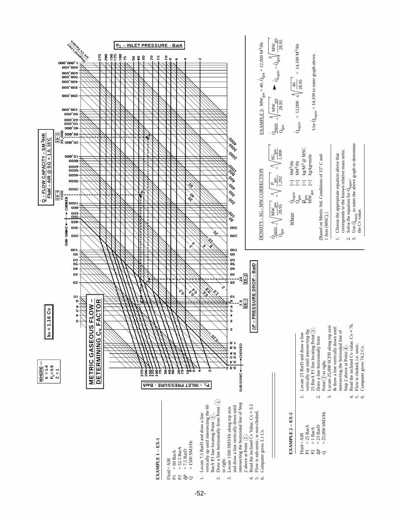
P – INLET PRESSURE - psia 1
P – INLET PRESSURE - psia 1
∆P
– P
RE
SS
UR
E D
RO
P -
psi
d
-52-
.
EX
AM
PLE
1 -
- E
X-1
Flu
id=
AIR
P1
= 6
0 B
arA
P2
= 5
2.5
Bar
A∆P
= 7
.5 B
arD
Q=
150
0 S
M3/
Hr
1.Lo
cate
7.5
Bar
D a
nd d
raw
a li
neve
rtic
ally
up
until
inte
rsec
ting
the
60B
arA
P1
line
loca
ting
Poi
nt
1 .
2.D
raw
a li
ne h
oriz
onta
lly fr
om P
oint
1
to r
ight
.3.
Loca
te 1
500
SM
3/H
r al
ong
top
axis
and
draw
a li
ne v
ertic
ally
dow
n un
tilin
ters
ectin
g th
e ho
rizon
tal l
ine
of S
tep
2 ab
ove
at P
oint
2
.4.
Rea
d th
e in
clin
ed C
v Va
lue.
Cv ≈ 3.
25.
Flo
w is
sub
-son
ic; i
e no
n-ch
oked
.6.
Com
pute
r gi
ves
3.1
Cv.
.
EX
AM
PLE
3:
MW
gas =
40,
Qga
s = 1
2,00
0 M3
/Hr
Qeq
uiv
=M
Wga
sQ
equi
v = Q
gas
MW
gas
Qga
s28
.95
28.9
5
Qeq
uiv
= 1
2,00
0 x
40=
14,
100
M3/H
r28
.95
Use
Qeq
uiv =
14,
100
to e
nter
gra
ph a
bove
.
.
. ..
.
.
.
EX
AM
PLE
2 -
- E
X-2
Flu
id=
AIR
1.Lo
cate
23
Bar
D a
nd d
raw
a li
neP
1=
25
Bar
Ave
rtic
ally
up
until
inte
rsec
ting
the
P2
= 1
Bar
A25
Bar
A P
1 lin
e lo
catin
g P
oint
3 .
∆P=
23
Bar
D2.
Dra
w a
line
hor
izon
tally
from
Q=
25,
000
SM
3/H
rP
oint
3 t
o rig
ht.
3.Lo
cate
25,
000
SC
FH
alo
ng to
p ax
is&
dra
w a
line
ver
tical
ly d
own
until
inte
rsec
ting
the
horiz
onta
l lin
e of
Ste
p 2
abov
e at
Poi
nt 4
.4.
Rea
d th
e in
clin
ed C
v va
lue.
Cv ≈ 76
.5.
Flo
w is
cho
ked;
i.e.
son
ic.
6.C
ompu
ter
give
s 74
.2 C
v.
.
DE
NS
ITY
- S
G -
MW
CO
RR
EC
TIO
N
Qeq
uiv
=M
Wga
s=
ρ gas
=S
Gga
s
Qga
s28
.95
1.29
21.
000
Whe
re:
Q equ
iv[=
]S
M3 /
Hr
Qga
s[=
]S
M3 /
Hr
ρ gas
[=]
kg/M
3 @
MS
CM
Wga
s[=
]kg
/kg•
mol
e
[Bas
ed o
n M
etric
Std
. Con
ditio
ns o
f 15
° C
and
1 A
tm (
MS
C).
]
1.C
hoos
e th
e ap
prop
riate
equ
atio
n ab
ove
that
corr
espo
nds
to th
e kn
own
rela
tive
mas
s un
its.
2.S
olve
the
equa
tion
for
Q equi
v.3.
Use
Qeq
uiv t
o en
ter
the
abov
e gr
aph
to d
eter
min
eth
e C
v va
lue.
. .
. .
..
0.10
0.2 0.3 0.
4
0.60.
8
1.0
2
34 6 810
20
3040
60
8010
0
200
300
400
600
1000
2000
3000
4000
800
Diago
nal L
ines
are C
v Facto
rs
Q –
FLO
W C
AP
AC
ITY
– S
M
/HR
Flu
id –
AIR
@ S
G =
1.0
, 15
°C3.
kv =
1.1
6 C
v
WH
ER
E —
k
= 1
.4
F =
0.9
Z
= 1
L
ME
TR
IC G
AS
EO
US
FLO
W –
DE
TE
RM
ININ
G C
F
AC
TO
Rv
P – INLET PRESSURE - BarA 1
SU
B-S
ON
ICC
HO
KE
D
∆P –
PR
ES
SU
RE
DR
OP
- B
arD
P – INLET PRESSURE - BarA1
-53-
.EX
AM
PLE
1 -
- E
X-1
Flu
id=
SAT
ST
M1.
Loca
te 1
10 p
sid
and
draw
a li
ne4.
Rea
d th
e in
clin
ed C
v va
lue.
Cv
≈ 10
0.P
1=
155
psi
ave
rtic
ally
up
until
inte
rsec
ting
the
5.F
low
is c
hoke
d; i.
e. s
onic
.P
2=
45
psia
155
psia
P1
line
loca
ting
Poi
nt 1
.6.
Com
pute
r gi
ves
102.
3 C
v.∆P
= 1
10 p
sia
2.D
raw
a li
ne h
oriz
onta
lly fr
omm
= 2
5,00
0 #/
Hr
Poi
nt 1
to
right
.T
1=
361
°F3.
Loca
te 2
5,00
0 #/
Hr
alon
g to
p ax
is&
dra
w a
line
ver
tical
ly d
own
until
inte
rsec
ting
the
horiz
onta
l lin
e of
Ste
p 2
abov
e at
Poi
nt 2
.
EX
AM
PLE
2 -
- E
X-2
Flu
id=
SA
T S
TM
1.Lo
cate
25
psid
and
dra
w a
line
4.R
ead
the
incl
ined
Cv
valu
e. C
v ≈
1.0.
P1
= 8
2 ps
iave
rtic
ally
up
until
inte
rsec
ting
the
5.F
low
is c
hoke
d; i.
e. s
onic
.P
2=
57
psia
82 p
sia
P1
line
loca
ting
Poi
nt 3
.6.
Com
pute
r gi
ves
1.22
Cv.
∆P=
25
psia
2.D
raw
a li
ne h
oriz
onta
lly fr
omm
= 1
40 #
/Hr
Poi
nt 3
to
right
.T
1=
314
°F3.
Loca
te 1
40 #
/Hr
alon
g to
p ax
is&
dra
w a
line
ver
tical
ly d
own
until
inte
rsec
ting
the
horiz
onta
l lin
e of
Ste
p 2
abov
e at
Poi
nt 4
.
.
0.01
0.10
0.20.3
0.4
0.50.7
1.0
23
45
710
20304050
70100
200300400500700 1000
Diagonal Lines are
CV Factors
EN
GLI
SH
–D
ET
ER
MIN
ING
Cv
FA
CT
OR
–
SA
TU
RA
TE
D S
TE
AM
– M
AS
S F
LOW
∆P
– P
RE
SS
UR
E D
RO
P -
psi
d
P – INLET PRESSURE – psia 1
P – INLET PRESSURE – psia1
m –
FLO
W C
AP
AC
ITY
– #
/HR
FLU
ID –
SA
TU
RA
TE
D S
TE
AM
. m –
FLO
W C
AP
AC
ITY
– #
/HR
FLU
ID –
SA
TU
RA
TE
D S
TE
AM
.
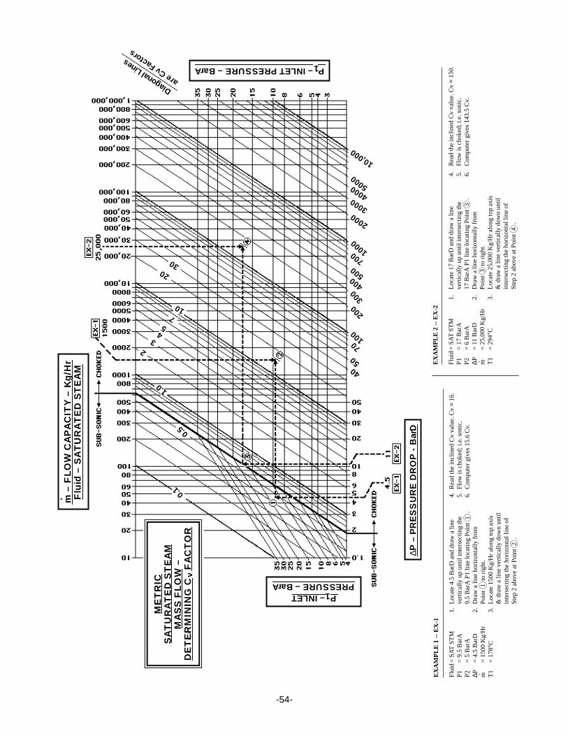
-54-
0.1
0.5
1.0
23
45
710
2030
4050
70
100
200
300
400 500700 1000
30004000 5000
10,000
ME
TR
ICS
AT
UR
AT
ED
ST
EA
MM
AS
S F
LOW
–D
ET
ER
MIN
ING
C
FA
CT
OR
v
m –
FLO
W C
AP
AC
ITY
– K
g/H
rF
luid
– S
AT
UR
AT
ED
ST
EA
M
.
∆P –
PR
ES
SU
RE
DR
OP
- B
arD
P – INLETPRESSURE – BarA
1
Diagonal Lines
are Cv Factors
P – INLET PRESSURE – BarA 1
2000
.EX
AM
PLE
1 -
- E
X-1
Flu
id=
SAT
ST
M1.
Loca
te 4
.5 B
arD
and
dra
w a
line
4.R
ead
the
incl
ined
Cv
valu
e. C
v ≈
16.
P1
= 9
.5 B
arA
vert
ical
ly u
p un
til in
ters
ectin
g th
e5.
Flo
w is
cho
ked;
i.e.
son
ic.
P2
= 5
Bar
A9.
5 B
arA
P1
line
loca
ting
Poi
nt 1
.6.
Com
pute
r gi
ves
15.6
Cv.
∆P=
4.5
Bar
D2.
Dra
w a
line
hor
izon
tally
from
m=
150
0 K
g/H
rP
oint
1 t
o rig
ht.
T1
= 1
78°C
3.Lo
cate
150
0 K
g/H
r al
ong
top
axis
& d
raw
a li
ne v
ertic
ally
dow
n un
tilin
ters
ectin
g th
e ho
rizon
tal l
ine
ofS
tep
2 ab
ove
at P
oint
2 .
EX
AM
PLE
2 -
- E
X-2
Flu
id=
SA
T S
TM
1.Lo
cate
17
Bar
D a
nd d
raw
a li
ne4.
Rea
d th
e in
clin
ed C
v va
lue.
Cv
≈ 15
0.P
1=
17
Bar
Ave
rtic
ally
up
until
inte
rsec
ting
the
5.F
low
is c
hoke
d; i.
e. s
onic
.P
2=
6 B
arA
17 B
arA
P1
line
loca
ting
Poi
nt 3
.6.
Com
pute
r gi
ves
143.
5 C
v.∆P
= 1
1 B
arD
2.D
raw
a li
ne h
oriz
onta
lly fr
omm
= 2
5,00
0 K
g/H
rP
oint
3 t
o rig
ht.
T1
= 2
94°C
3.Lo
cate
25,
000
Kg/
Hr
alon
g to
p ax
is&
dra
w a
line
ver
tical
ly d
own
until
inte
rsec
ting
the
horiz
onta
l lin
e of
Ste
p 2
abov
e at
Poi
nt 4
.
.
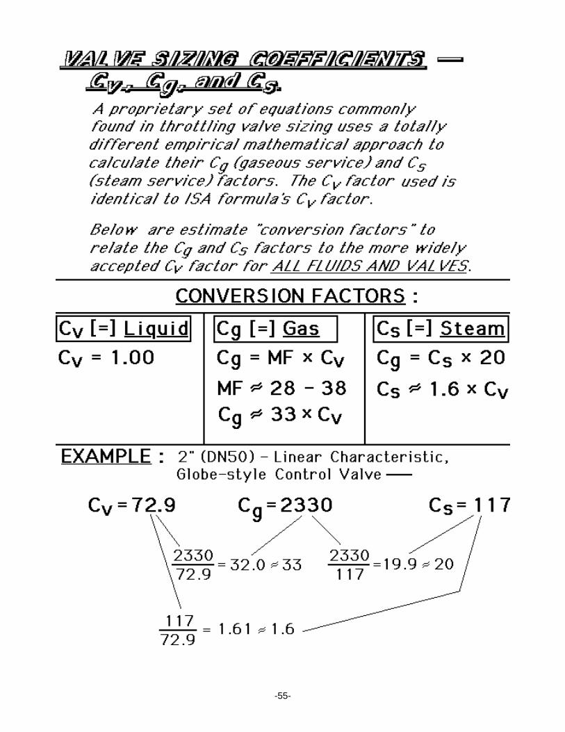
-55-

• 607 West 15th Street • P.O. Box 6 • Ellsworth, KS 67439-0006• PH: (785) 472-4461 • FAX: (785) 472-3539 (domestic) or (785) 472-8544 (exports)
• E-mail: [email protected] or [email protected]


![Fluid Flow[1]](https://img.pdfslide.net/doc/110x75/577d38c01a28ab3a6b986b59/fluid-flow1.jpg)