Fluid flow in curved geometries:Mathematical Modeling and ApplicationsFluid flow in curved geometries:Mathematical Modeling and Applications

Dr. Muhammad Sajid

Theoretical Plasma Physics DivisionPINSTECH, P.O. Nilore, PAEC, Islamabad

March 01-06, 2010Islamabad, Pakistan

Presentation Layout

Analysis of fluid behaviour

Governing equations

Manifold and Metric

∇ operations

Stretching a curved surface

Peristaltic flow in a curved channel

Summary

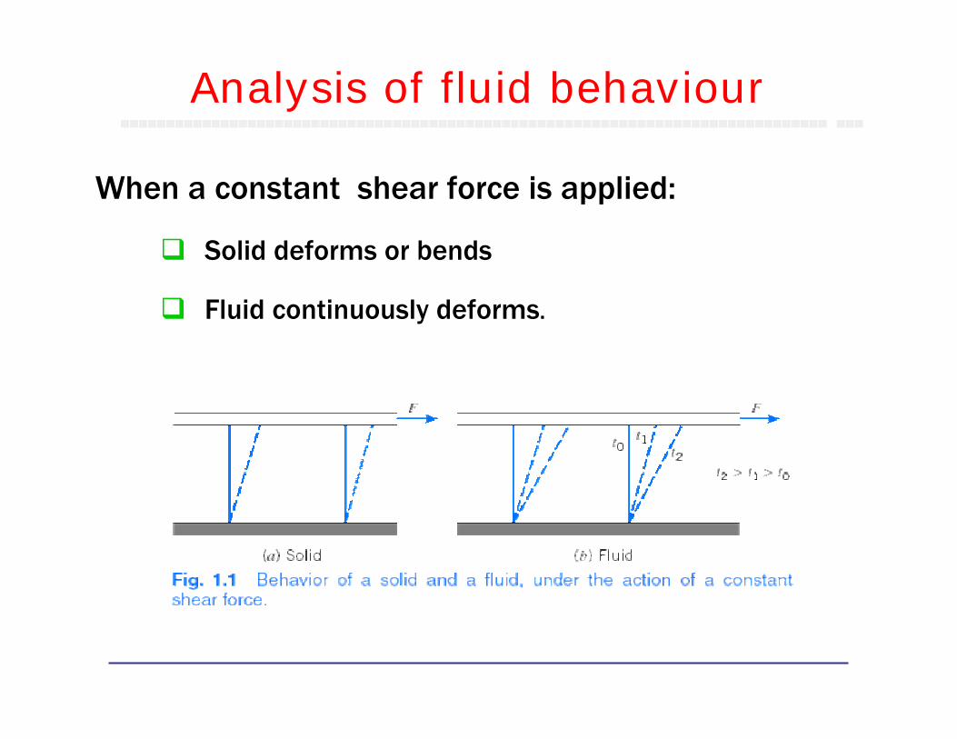
When a constant shear force is applied:

Solid deforms or bends

Fluid continuously deforms.

Analysis of fluid behaviour

Analysis of fluid behaviour

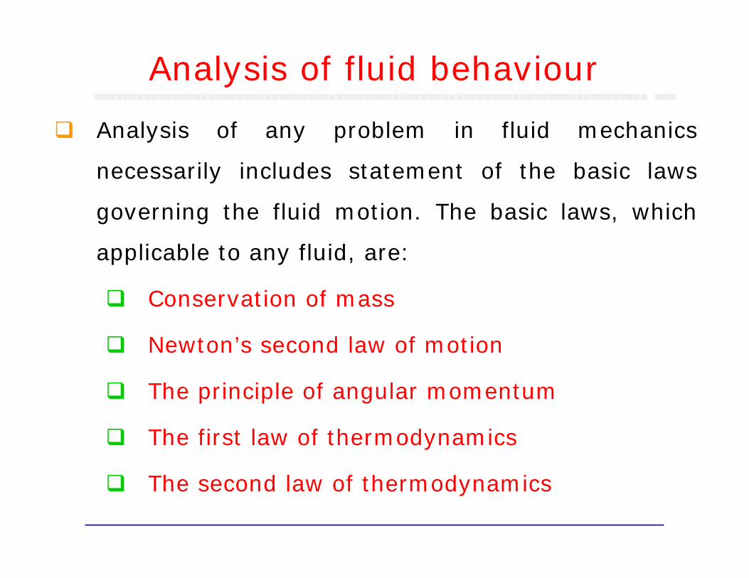
Analysis of any problem in fluid mechanics

necessarily includes statement of the basic laws

governing the fluid motion. The basic laws, which

applicable to any fluid, are:

Conservation of mass

Newton’s second law of motion

The principle of angular momentum

The first law of thermodynamics

The second law of thermodynamics

NOT all basic laws are required to solve any one

problem. On the other hand, in many problems it

is necessary to bring into the analysis additional

relations that describe the behavior of physical

properties of fluids under given conditions.

Many apparently simple problems in fluid

mechanics that cannot be solved analytically.

In such cases we must resort to more

complicated numerical solutions and/or

results of experimental tests.

Analysis of fluid behaviour

Governing Equations

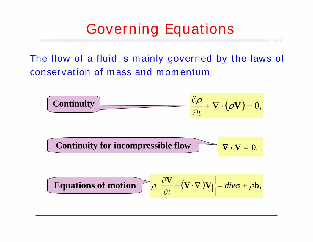
Continuity

Equations of motion

Continuity for incompressible flow

( ) ,0=⋅+∂∂ Vρρ

∇t

∇ V 0.

( ) ,bVVV ρρ +σ∇ divt

=⎥⎦⎤

⎢⎣⎡ ⋅+∂∂

The flow of a fluid is mainly governed by the laws of conservation of mass and momentum

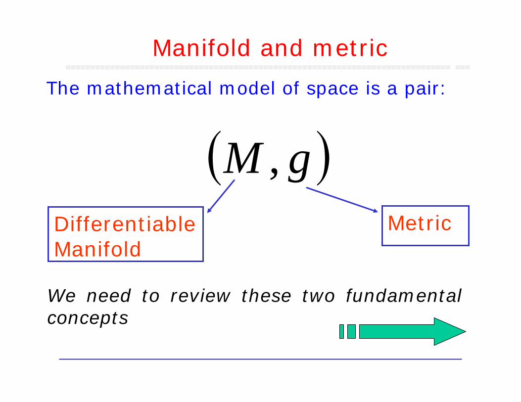
Manifold and metric

The mathematical model of space is a pair:

( )gM ,Differentiable Manifold

Metric

We need to review these two fundamentalconcepts

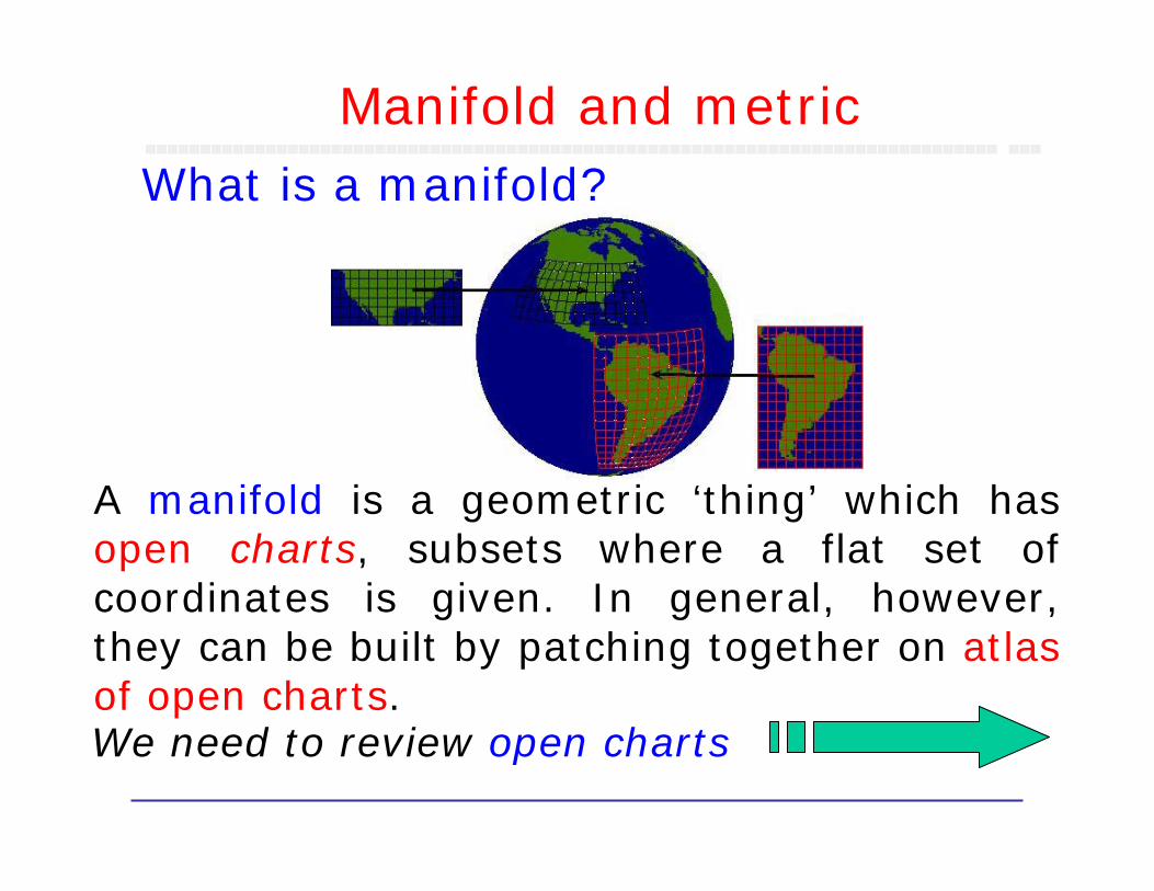
Manifold and metricWhat is a manifold?

A manifold is a geometric ‘thing’ which has open charts, subsets where a flat set of coordinates is given. In general, however, they can be built by patching together on atlas of open charts.We need to review open charts

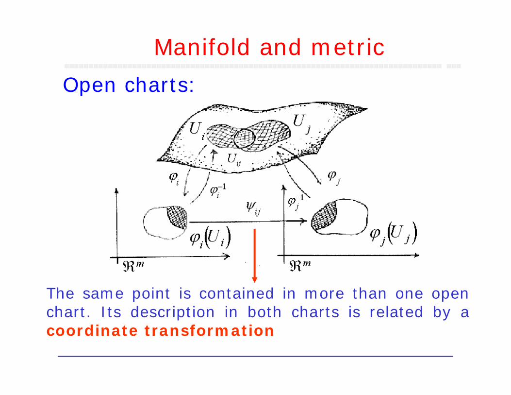
Manifold and metric

Open charts:

The same point is contained in more than one open chart. Its description in both charts is related by a coordinate transformation

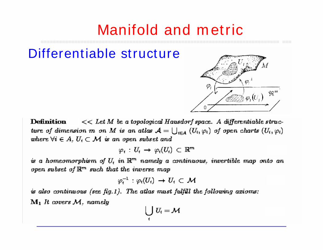
Manifold and metric

Differentiable structure

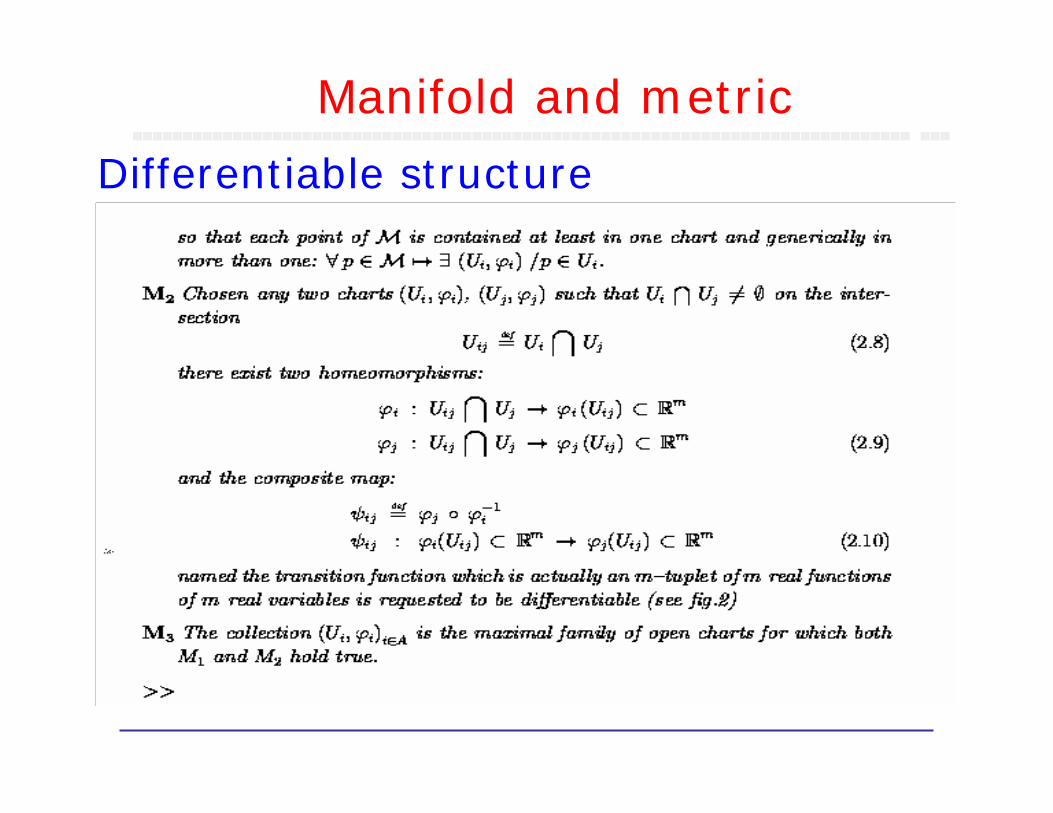
Manifold and metric

Differentiable structure

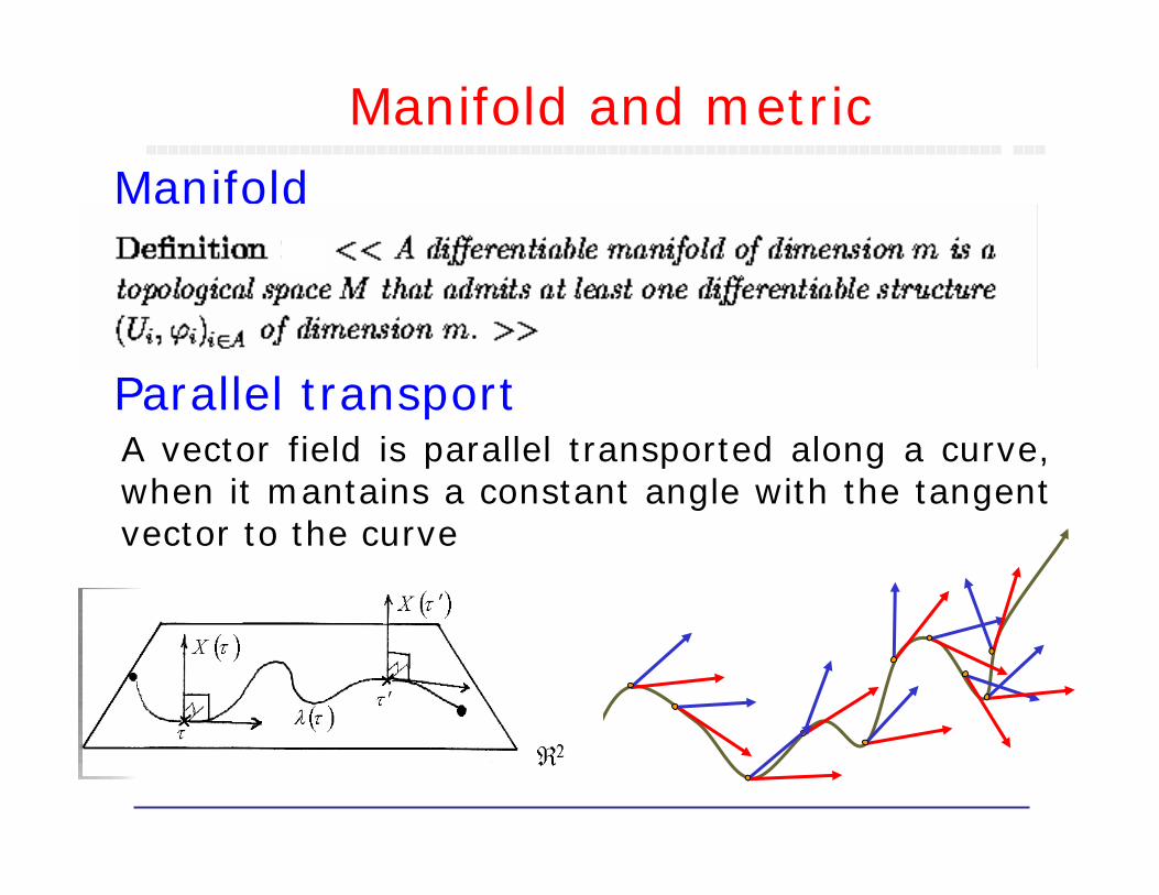
Manifold and metricManifold

Parallel transportA vector field is parallel transported along a curve, when it mantains a constant angle with the tangent vector to the curve

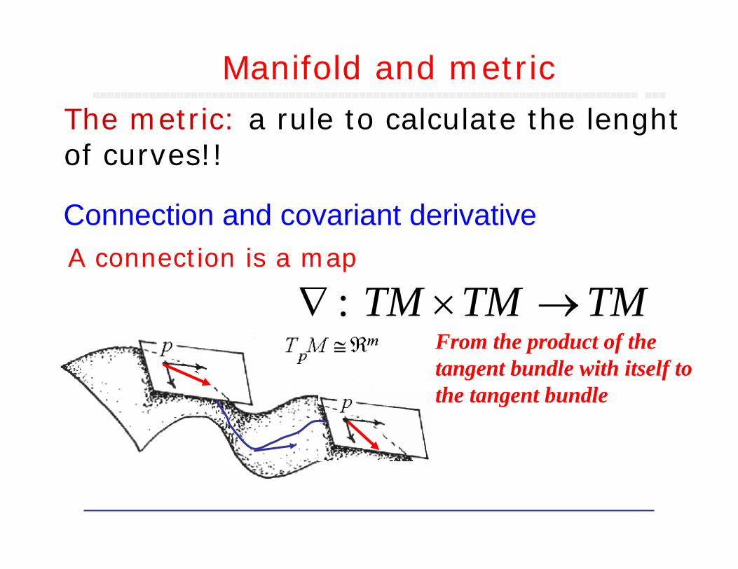
Manifold and metricThe metric: a rule to calculate the lenghtof curves!!

Connection and covariant derivative

TMTMTM →×∇ :A connection is a map

From the product of the tangent bundle with itself to the tangent bundle

14Fluid Mechanics Group (FMG)

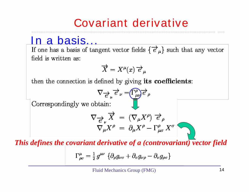
In a basis...

This defines the covariant derivative of a (controvariant) vector field

Covariant derivative

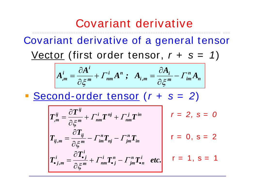
Covariant derivative of a general tensorVector (first order tensor, r + s = 1)

AAA ; AAA nn

immi

m,ini

nmm

iim, Γ

ξΓ

ξ−

∂∂

=+∂∂

=

Second-order tensor (r + s = 2)

etc. TTT

T

TTT

T

TTTT

in

njm

nj

inmm

iji

m,j

innjmnj

nimm

ijm,ij

injnm

njinmm

ijijm,

•••

• −+∂∂

=

−−∂∂

=

++∂∂

=

ΓΓξ

ΓΓξ

ΓΓξ

r = 2, s = 0

r = 0, s = 2

r = 1, s = 1

Covariant derivative

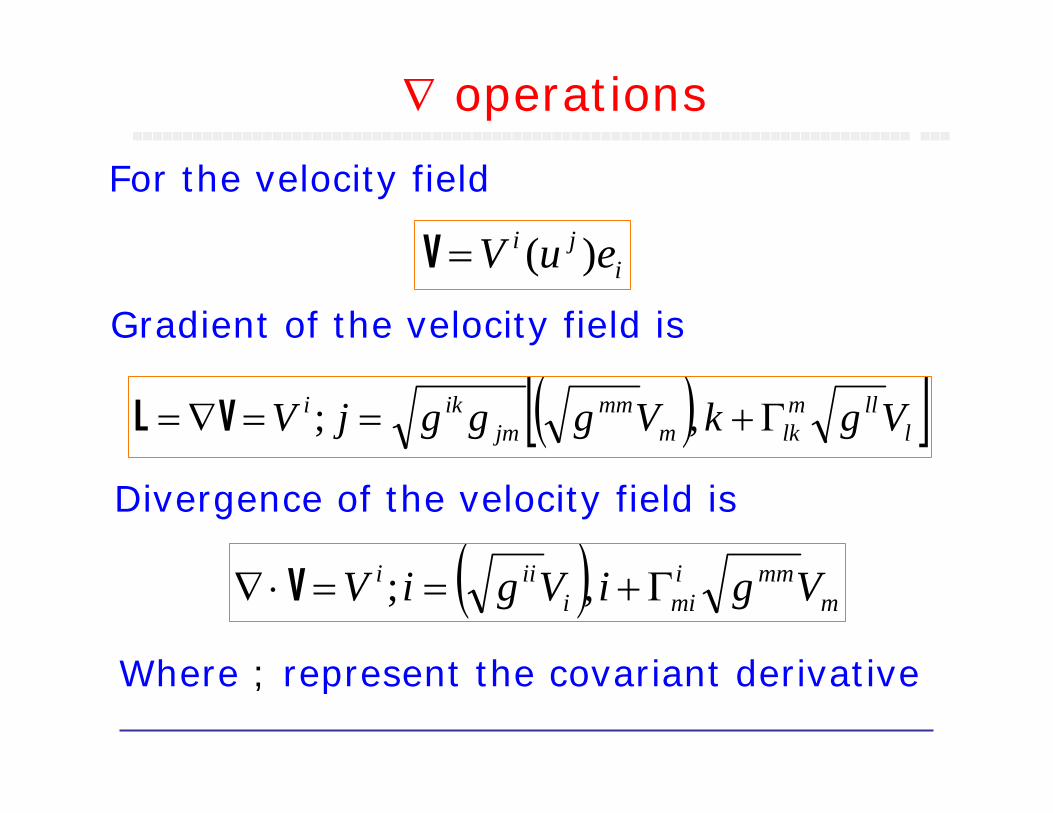
For the velocity field

iji euV )(=V

( ) mmmi

miiiii VgiVgiV Γ+==⋅∇ ,;V

Gradient of the velocity field is

Where ; represent the covariant derivative

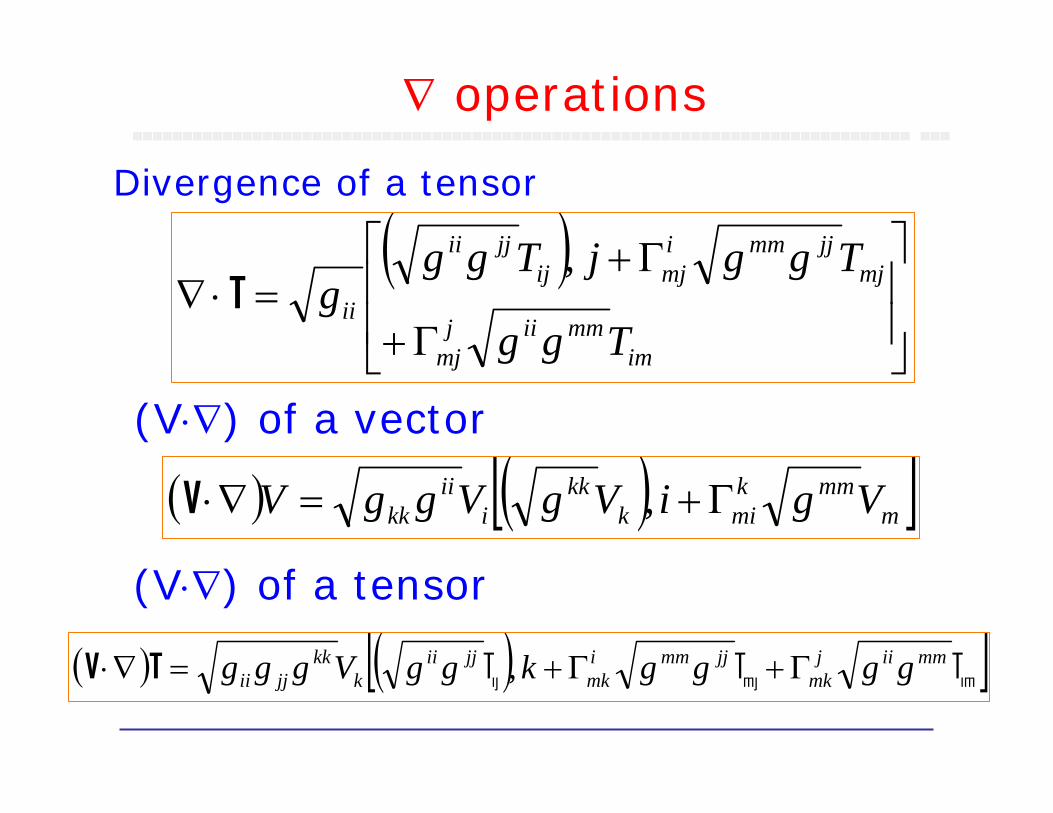
∇ operations

( )[ ]lllmlkm

mmjm

iki VgkVgggjV Γ+==∇= ,;VL

Divergence of the velocity field is

( ) ( )[ ]immjij TTT mmiijmk

jjmmimk

jjiik

kkjjii ggggkggVggg Γ+Γ+=∇⋅ ,TV

Divergence of a tensor

( )⎥⎥

⎦

⎤

⎢⎢

⎣

⎡

Γ+

Γ+=⋅∇

immmiij

mj

mjjjmmi

mjijjjii

iiTgg

TggjTggg

,T

( ) ( )[ ]mmmk

mikkk

iii

kk VgiVgVggV Γ+=∇⋅ ,V

∇ operations

(V⋅∇) of a vector

(V⋅∇) of a tensor

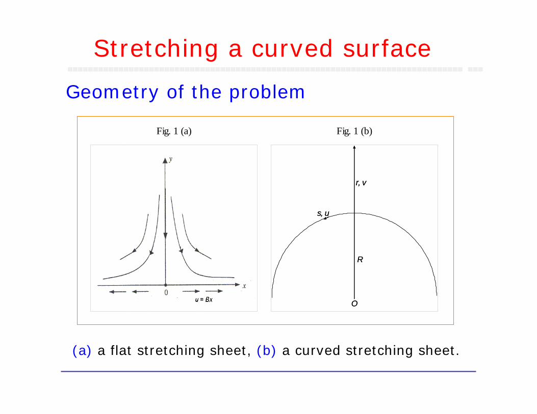
Stretching a curved surface

Fig. 1 (a) Fig. 1 (b)

R

r, v

s, u

O

R

r, v

s, u

O

(a) a flat stretching sheet, (b) a curved stretching sheet.

Geometry of the problem

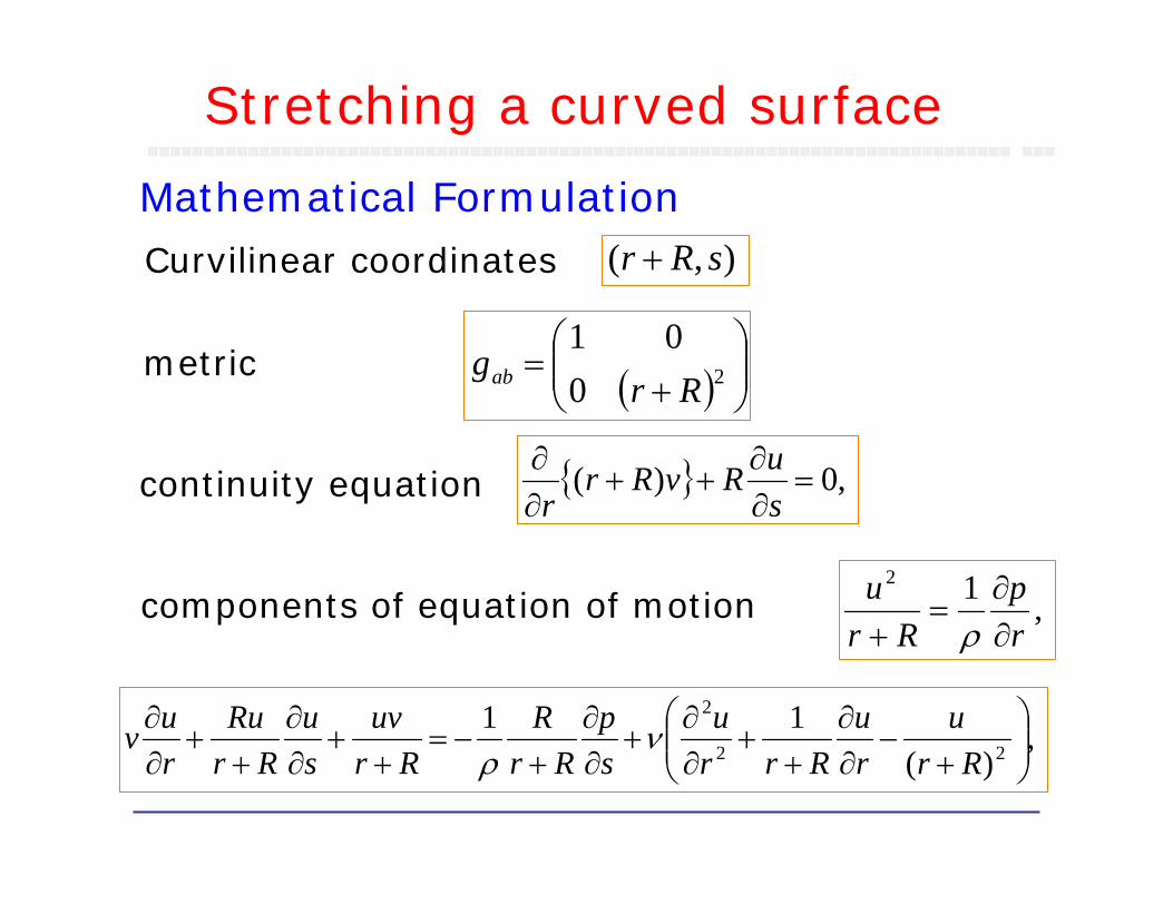
Stretching a curved surface

Mathematical Formulation),( sRr +

,)(

1122

2

⎟⎟⎠

⎞⎜⎜⎝

⎛+

−∂∂

++

∂∂

+∂∂

+−=

++

∂∂

++

∂∂

Rru

ru

Rrru

sp

RrR

Rruv

su

RrRu

ruv ν

ρ

,12

rp

Rru

∂∂

=+ ρ

( ) ⎟⎟⎠⎞

⎜⎜⎝

⎛+

= 2001Rr

gab

Curvilinear coordinates

metric

{ } ,0)( =∂∂

++∂∂

suRvRr

rcontinuity equation

components of equation of motion

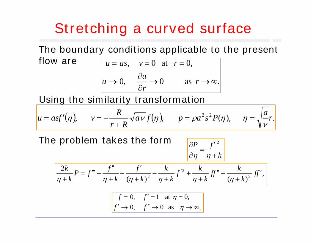
Stretching a curved surfaceThe boundary conditions applicable to the present flow are

Using the similarity transformation

The problem takes the form

. as 0 ,0

,0at 0 ,

∞→→∂∂

→

===

rruu

rvasu

( ) ( ) . ,)( , , 22 raPsapfaRr

Rvfasuν

ηηρηνη ==+

−=′=

kfP+′

=∂∂

ηη

2

,)()(

22

22 ff

kkff

kkf

kk

kf

kffP

kk ′

++′′

++

+−

+′

−+′′

+′′′=+

′

ηηηηηη

, as 0 ,0,0at 1 ,0∞→→′′→′

==′=η

ηffff

Stretching a curved surface

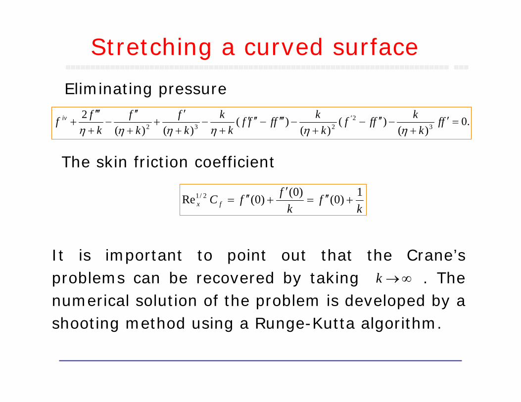
Eliminating pressure

It is important to point out that the Crane’s problems can be recovered by taking . The numerical solution of the problem is developed by a shooting method using a Runge-Kutta algorithm.

The skin friction coefficient

.0)(

)()(

)()()(

23

2232 =′

+−′′−

+−′′′−′′′

+−

+′

++′′

−+′′′

+ ′ ffk

kfffk

kffffk

kk

fk

fk

ff iv

ηηηηηη

kf

kffC fx

1)0()0()0(Re 2/1 +′′=′

+′′=

∞→k

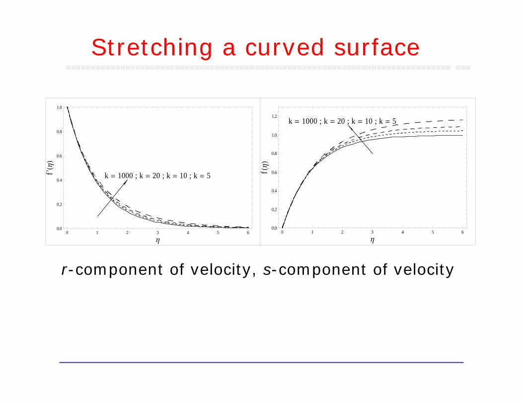
Stretching a curved surface

r-component of velocity, s-component of velocity

0 1 2 3 4 5 60.0

0.2

0.4

0.6

0.8

1.0

h

f'HhL

k = 1000 ; k = 20 ; k = 10 ; k = 5

0 1 2 3 4 5 60.0

0.2

0.4

0.6

0.8

1.0

1.2

h

fHhL

k = 1000 ; k = 20 ; k = 10 ; k = 5

Stretching a curved surface

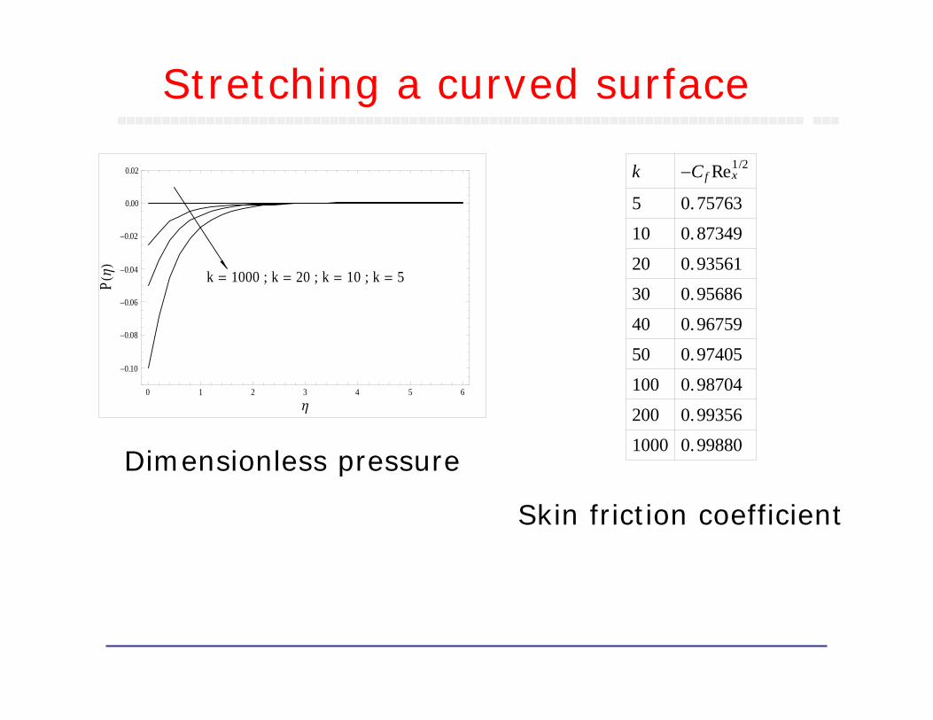
Dimensionless pressure

0 1 2 3 4 5 6

-0.10

-0.08

-0.06

-0.04

-0.02

0.00

0.02

h

PHhL k = 1000 ; k = 20 ; k = 10 ; k = 5

k −Cf Rex1/2

5 0.75763

10 0.87349

20 0.93561

30 0.95686

40 0.96759

50 0.97405

100 0.98704

200 0.99356

1000 0.99880

Skin friction coefficient

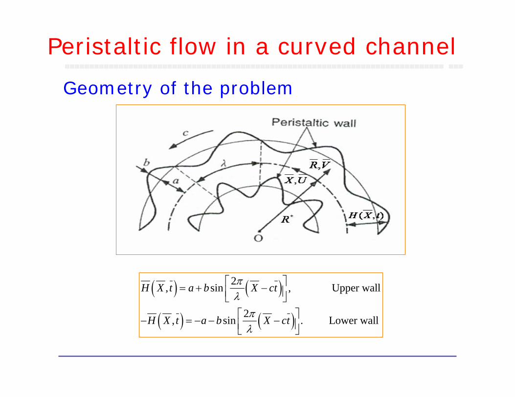
Peristaltic flow in a curved channel

Geometry of the problem

( ) ( )

( ) ( )

2, sin , Upper wall

2, sin . Lower wall

H X t a b X ct

H X t a b X ct

πλ

πλ

⎡ ⎤= + −⎢ ⎥⎣ ⎦⎡ ⎤− = − − −⎢ ⎥⎣ ⎦

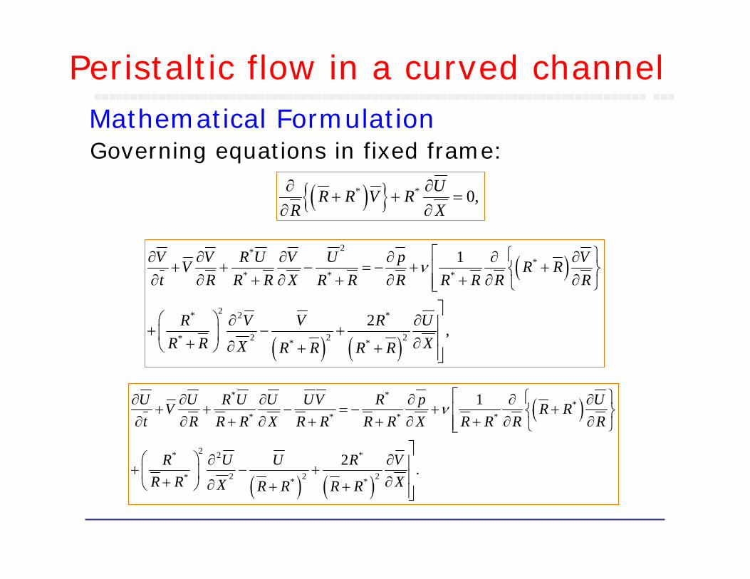
Peristaltic flow in a curved channelMathematical FormulationGoverning equations in fixed frame:

( ){ }* * 0,UR R V RR X∂ ∂

+ + =∂ ∂

( )

( ) ( )

2**

* * *

2* 2 *

2 2 2* * *

1

2 ,

V V R U V U p VV R Rt R R R X R R R R R R R

R V V R UR R XX R R R R

ν⎡ ⎧ ⎫∂ ∂ ∂ ∂ ∂ ∂

+ + − = − + +⎢ ⎨ ⎬∂ ∂ + ∂ + ∂ + ∂ ∂⎢ ⎩ ⎭⎣

⎤⎛ ⎞ ∂ ∂ ⎥+ − +⎜ ⎟ ⎥+ ∂⎝ ⎠ ∂ + + ⎥⎦

( )

( ) ( )

* **

* * * *

2* 2 *

2 2 2* * *

1

2 .

U U R U U UV R p UV R Rt R R R X R R R R X R R R R

R U U R VR R XX R R R R

ν⎡ ⎧ ⎫∂ ∂ ∂ ∂ ∂ ∂

+ + − = − + +⎢ ⎨ ⎬∂ ∂ + ∂ + + ∂ + ∂ ∂⎢ ⎩ ⎭⎣

⎤⎛ ⎞ ∂ ∂ ⎥+ − +⎜ ⎟ ⎥+ ∂⎝ ⎠ ∂ + + ⎥⎦

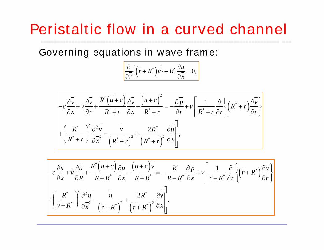
Peristaltic flow in a curved channelGoverning equations in wave frame:

( ){ }* * 0,ur R v Rr x∂ ∂

+ + =∂ ∂

( ) ( ) ( )

( ) ( )

2**

* * *

2* 2 *

2 2 2* * *

1

2 ,

R u c u cv v v p vc v R rx r R r x R r r R r r r

R v v R uR r xx R r R r

ν+ + ⎡ ⎧ ⎫∂ ∂ ∂ ∂ ∂ ∂

− + + − = − + +⎢ ⎨ ⎬∂ ∂ + ∂ + ∂ + ∂ ∂⎢ ⎩ ⎭⎣

⎤⎛ ⎞ ∂ ∂ ⎥+ − +⎜ ⎟ ⎥+ ∂⎝ ⎠ ∂ + + ⎥⎦

( ) ( ) ( )

( ) ( )

* **

* * * *

2* 2 *

2 2 2* * *

1

2 .

R u c u c vu u u R p uc v r Rx R R R x R R R R x r R r r

R u u R vv R xx r R r R

ν+ + ⎡ ⎧ ⎫∂ ∂ ∂ ∂ ∂ ∂

− + + − = − + +⎢ ⎨ ⎬∂ ∂ + ∂ + + ∂ + ∂ ∂⎢ ⎩ ⎭⎣

⎤⎛ ⎞ ∂ ∂ ⎥+ − +⎜ ⎟ ⎥+ ∂⎝ ⎠ ∂ + + ⎥⎦

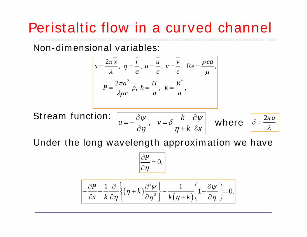
Peristaltic flow in a curved channelNon-dimensional variables:

Stream function: 2 .aπδλ

=where

2 *

2 , , , , Re ,

2 , , ,

x r u v cax u va c c

a H RP p h kc a a

π ρηλ µ

πλµ

= = = = =

= = =

, ku vk x

ψ ψδη η

∂ ∂= − =

∂ + ∂

Under the long wavelength approximation we have

0,Pη∂

=∂

( ) ( )2

2

1 1 1 0.P kx k k k

ψ ψηη η η η⎧ ⎫ ⎛ ⎞∂ ∂ ∂ ∂

− − + − − =⎨ ⎬ ⎜ ⎟∂ ∂ ∂ + ∂⎝ ⎠⎩ ⎭

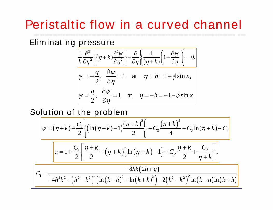
Peristaltic flow in a curved channelEliminating pressure

( ) ( )2 2

2 2

1 1 1 0.kk k

ψ ψηη η η η η

⎧ ⎫⎧ ⎫ ⎛ ⎞∂ ∂ ∂ ∂⎪ ⎪+ + − =⎨ ⎬ ⎨ ⎬⎜ ⎟∂ ∂ ∂ + ∂⎝ ⎠⎪ ⎪⎩ ⎭ ⎩ ⎭

, 1 at 1 sin ,2

, 1 at 1 sin ,2

q h x

q h x

ψψ η φη

ψψ η φη

∂= − = = = +

∂∂

= = = − = − −∂

Solution of the problem

( ) ( )( ) ( ) ( ) ( )2 2

12 3 4ln 1 ln

2 2 4k kCk k C C k C

η ηψ η η η

⎧ ⎫+ +⎪ ⎪= + + + − + + + +⎨ ⎬⎪ ⎪⎩ ⎭

( ) ( ){ } 3121 ln 1 .

2 2 2CC k ku k k C

kη ηη η

η⎡ ⎤+ +

= + + + + − + +⎢ ⎥+⎣ ⎦

( )( ) ( ) ( )( ) ( ) ( ) ( )

1 2 22 22 2 2 2 2 2

8 2

4 ln ln 2 ln ln

hk h qC

h k h k k h k h h k k h k h

− +=− + − − + + − − − +

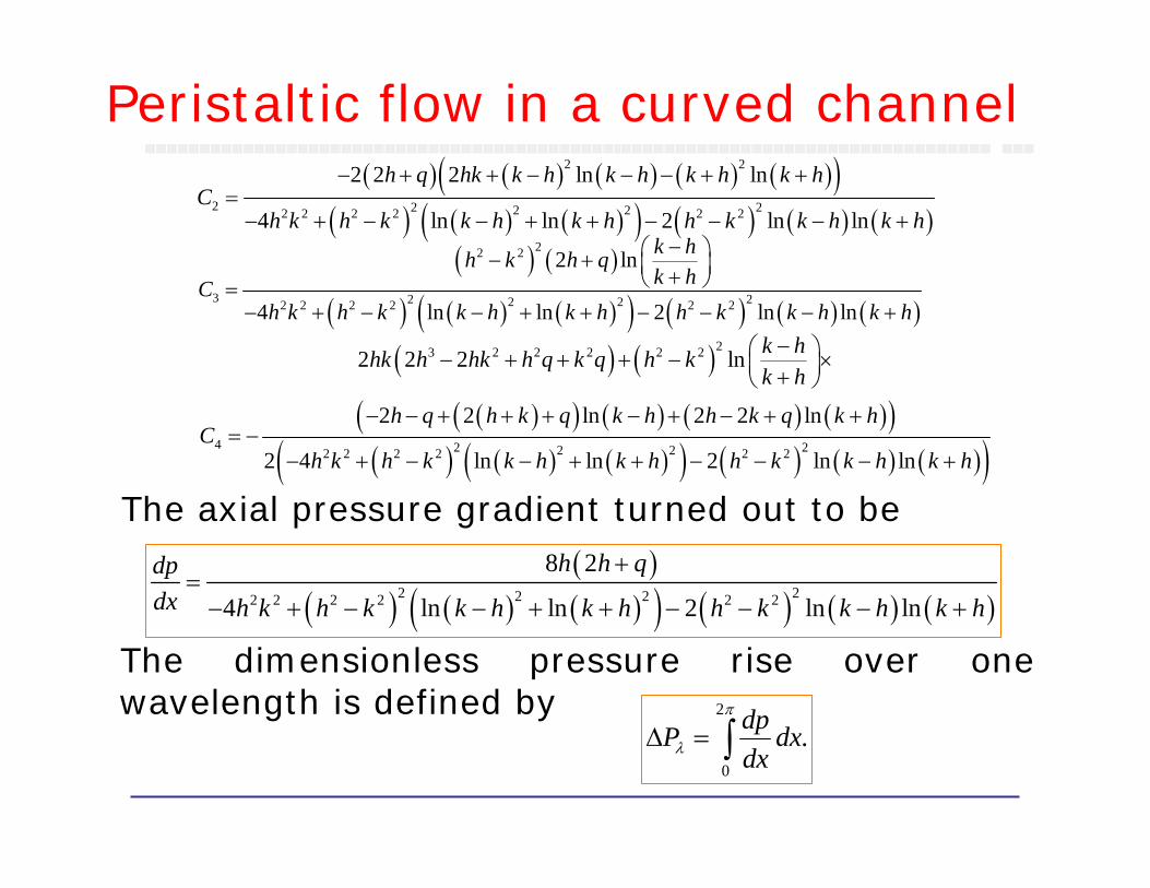
Peristaltic flow in a curved channel

The axial pressure gradient turned out to be( )

( ) ( ) ( )( ) ( ) ( ) ( )2 22 22 2 2 2 2 2

8 2

4 ln ln 2 ln ln

h h qdpdx h k h k k h k h h k k h k h

+=− + − − + + − − − +

The dimensionless pressure rise over one wavelength is defined by 2

0

.dpP dxdx

π

λ∆ = ∫

( ) ( ) ( ) ( ) ( )( )( ) ( ) ( )( ) ( ) ( ) ( )

2 2

2 2 22 22 2 2 2 2 2

2 2 2 ln ln

4 ln ln 2 ln ln

h q hk k h k h k h k hC

h k h k k h k h h k k h k h

− + + − − − + +=− + − − + + − − − +

( ) ( )

( ) ( ) ( )( ) ( ) ( ) ( )

22 2

3 2 22 22 2 2 2 2 2

2 ln

4 ln ln 2 ln ln

k hh k h qk hC

h k h k k h k h h k k h k h

−⎛ ⎞− + ⎜ ⎟+⎝ ⎠=− + − − + + − − − +

( ) ( )( )( ) ( ) ( ) ( )( )

( ) ( ) ( )( ) ( ) ( ) ( )( )

23 2 2 2 2 2

4 2 22 22 2 2 2 2 2

2 2 2 ln

2 2 ln 2 2 ln

2 4 ln ln 2 ln ln

k hhk h hk h q k q h kk h

h q h k q k h h k q k hC

h k h k k h k h h k k h k h

−⎛ ⎞− + + + − ×⎜ ⎟+⎝ ⎠

− − + + + − + − + += −

− + − − + + − − − +

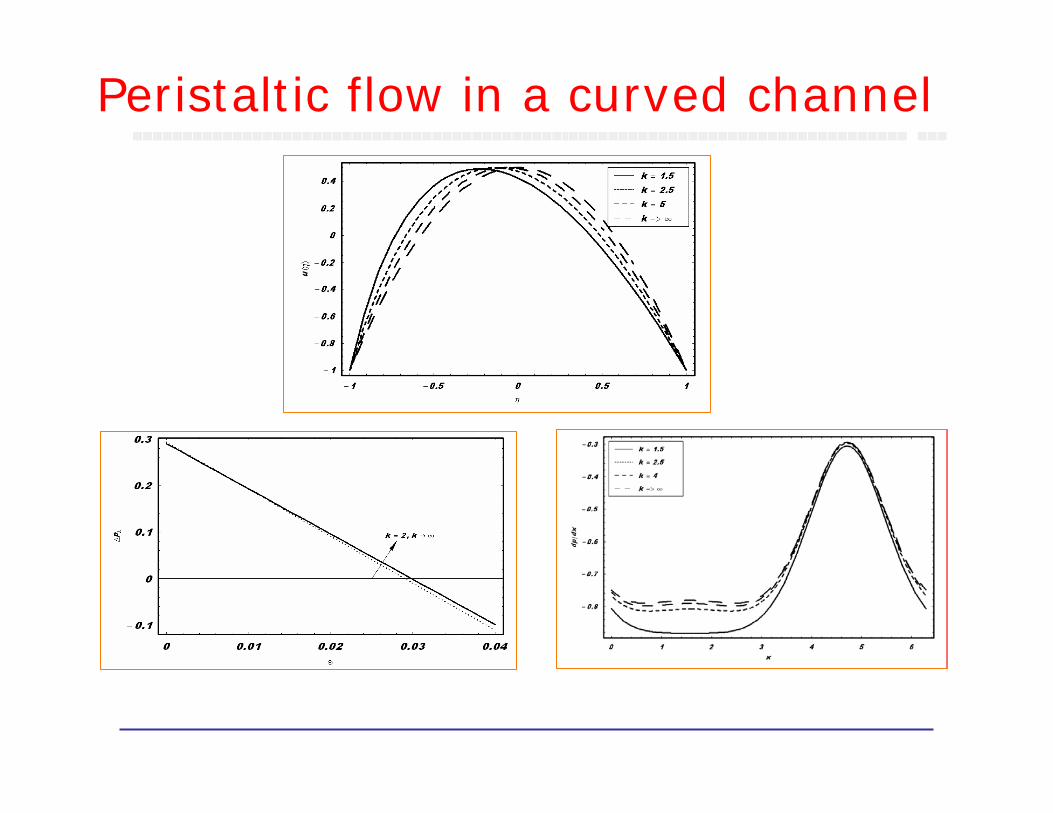
Peristaltic flow in a curved channel

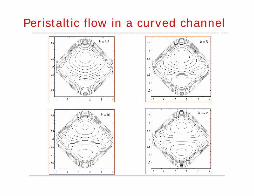
Peristaltic flow in a curved channel3.5k = 5k =

10k = k →∞

Summary

The ∇ operations for curvilinear

coordinates have been discussed.

Flow of a viscous fluid due to

Stretching a curved surface is

analyzed.

Peristaltic flow in a curved channel is

investigated.

Thank You!