Research Collection

Doctoral Thesis

Fluid-mechanical model for vestibular responses to sound inpresence of a superior canal dehiscence

Author(s): Grieser, Bernhard Johann

Publication Date: 2015

Permanent Link: https://doi.org/10.3929/ethz-a-010443913

Rights / License: In Copyright - Non-Commercial Use Permitted

This page was generated automatically upon download from the ETH Zurich Research Collection. For moreinformation please consult the Terms of use.

ETH Library

Flu

id-M

ec

ha

nic

al

Mo

de

l fo

r V

estib

ula

r R

esp

on

se

s t

o S

ou

nd

in

Pre

se

nc

e o

f a

Su

pe

rio

r C

an

al

De

his

ce

nc

e

Be

rn

ha

rd

Grie

se

r

Patients with a superior canal dehiscence (SCD) in the inner ear suffer from events

of dizziness and vertigo in response to sound, also known as Tullio phenomenon

(TP). To date, the mechanisms behind TP remain obscure. When risky surgical

interventions appear to be the only means to cure the symptoms, it may be

worthwhile to study the underlying mode of operation and possibly devise less

invasive methods.

Approaching this medical condition from an engineering perspective, we are

faced with an intertwined system of fluids (endolymph and perilymph), elastic

structures (membranous labyrinth, cupula, dehiscence) and rigid bone (temporal

bone, stapes). In accordance with the so-called ‘third window theory’, we assume

that the vibrating stapes causes abnormal perilymph pulsations towards the

pathologic ‘window’ in the superior canal of the balance sense. Based on this

assumption, we developed a computational model in order to resolve fluid-

structure interactions which we expect to arise from such a coupled system.

The simulation results confirm our hypothesis, revealing the occurrence of wave

propagation phenomena along the deforming membranous canal. More

specifically, we note that two substantially different flows are evolving. First, the

deforming labyrinth causes pulsations of the endolymph which lead to rapid

vibrations of the cupula in phase with the sound stimulus. Second, these primary

pulsations feature a static component, the so-called steady streaming, such that

endolymph is continuously driven through the canals in (mostly) ampullofugal

direction. Reaching a quasi-steady balance with the opposing cupula, the latter

maintains a constant deflection amplitude. Both findings are in agreement with

clinical observations on the cupula response in patients with SCD.

Carrying out a sensitivity study, we were able to obtain an analytical fit to match

our simulation results in a relevant range of parameters. We coupled the inner-ear

dynamics to the corresponding eye response (vestibulo-ocular reflex). The results

reveal a ‘sweet spot’ for TP within the audible spectrum which largely coincides

with patient data. We found that the underlying mechanisms originate primarily

from Reynolds stresses in the fluid, which are weakest in the lower sound

spectrum. Additionally, natural variations in the membrane stiffness and the

stapes motility are observed to shift the sweet spot. Waves become evanescent

above 4-6kHz, such that we cannot expect vestibular responses in that range.

FLUID-MECHANICAL MODEL FOR

VESTIBULAR RESPONSES TO SOUND IN PRESENCE OF A

SUPERIOR CANAL DEHISCENCE

Bernhard Grieser

Dissertation ETH No. 22681

Summary

Cover: Illustration of the dehiscent superior canal within thevestibular system of the inner ear; see also Fig. 3.1 on p. 30.

An electronic version of this thesis may be downloaded fromhttp://dx.doi.org/10.3929/ethz-a-010443913.

Diss. ETH No. 22681

FLUID-MECHANICAL MODEL

FOR

VESTIBULAR RESPONSES TO SOUND

IN PRESENCE OF A

SUPERIOR CANAL DEHISCENCE

A thesis submitted to attain the degree of

DOCTOR OF SCIENCES of ETH ZURICH

(Dr. sc. ETH Zurich)

presented by

Bernhard Johann Grieser

Dipl.-Ing., Karlsruhe Institute of Technology (KIT)born on March 4, 1986

citizen of Germany

accepted on the recommendation of

Prof. Dr. L. Kleiser, examinerProf. Dr. D. Obrist, co-examinerProf. Dr. J. Dual, co-examiner

2015

Abstract

Patients with a superior canal dehiscence (SCD) in the inner earsuffer from events of dizziness and vertigo in response to sound, alsoknown as Tullio phenomenon (TP). To date, the mechanisms behind thisphenomenon remain obscure. When risky surgical interventions appearto be the only means to cure the symptoms, it may be worthwhile tostudy the underlying mode of operation and possibly devise less invasivemethods.

Approaching this medical condition from an engineering perspective,we are faced with an intertwined system of fluids (endolymph and per-ilymph), elastic structures (membranous labyrinth, cupula, dehiscence)and rigid bone (temporal bone, stapes). In accordance with the so-called ‘third window theory’, we assume that the vibrating stapes causesabnormal perilymph pulsations towards the pathologic ‘window’ in thesuperior canal of the balance sense. Based on this primary assumption,we developed a computational model in order to resolve fluid-structureinteractions which we expect to arise from such a coupled system. We dis-cretize our computational domain using the Finite-Volume Method andsolve the fluid motion with the Navier-Stokes equations in the ArbitraryLagrangian-Eulerian (ALE) formulation for moving grids. The dynamicsof the embedded membranous labyrinth is considered by a linear-elasticshell model and coupled to the adjacent fluids by an iterative procedureusing Aitken relaxation. The cupula dynamics follows a volume-basedformulation. Our model is implemented in C++ by a tailor-made codeusing the open source libraries of OpenFOAM and Armadillo.

The simulation results confirm our hypothesis, revealing the occur-rence of wave propagation phenomena along the deforming membranouscanal. More specifically, we note that two substantially different flowsare evolving. First, the deforming labyrinth causes pulsations of the en-dolymph which lead to rapid vibrations of the cupula, both in phasewith the sound stimulus. Second, these primary pulsations feature astatic component, the so-called steady streaming, such that endolymphis continuously driven through the canals in (mostly) ampullofugal di-rection. Reaching a quasi-steady balance with the opposing cupula, thelatter maintains a constant deflection amplitude. Both findings are inagreement with clinical observations on the cupula response in patientswith SCD.

Carrying out a sensitivity study and employing dimensional analysis,we are able to obtain an analytical fit to match our simulation results

in a relevant range of parameters. Through the vestibulo-ocular reflex,the eyes are moving at a speed and direction which corresponds to thecupula displacement and the plane of the superior canal, respectively.We thus coupled the inner-ear dynamics to the corresponding eye mo-tion by means of lumped parameters. The results reveal a ‘sweet spot’for the Tullio phenomenon within the audible spectrum which largelycoincides with patient data from the literature. We find that the un-derlying mechanisms originate primarily from Reynolds stresses in thefluid, which are weakest in the lower sound spectrum. Additionally, nat-ural variations in the membrane stiffness and the stapes motility areobserved to shift the sweet spot on the frequency scale. Waves becomeevanescent at frequencies above about 4 − 6kHz, such that we cannotexpect vestibular responses in that range.

Kurzfassung

Patienten, die eine Dehiszenz im oberen Bogengang des Innenohrsaufweisen, leiden gewöhnlich an Schall-induzierten Drehschwindelat-tacken, auch bekannt als Tullio-Phänomen. Bisher konnten dessen Hin-tergründe nicht ausreichend geklärt werden. Da die zur Behandlungnotwendigen Operationen sehr risikoreich sind, könnte es sich lohnen, dieFunktionsweise des Phänomens zu erforschen, um aus den gewonnenenErkenntnissen möglicherweise weniger invasive Verfahren abzuleiten.

Indem wir das Krankheitsbild aus der Sichtweise eines Inge-nieurs betrachten, identifizieren wir zunächst ein verwobenes Systemaus Flüssigkeiten (Endolymphe und Perilymphe), elastischen Struk-turen (häutiges Labyrinth, Cupula, Dehiszenz) sowie festem Knochen(Schläfenbein, Steigbügel). In Einklang mit der sogenannten ‘Theorie desdritten Fensters’ vermuten wir, dass der Steigbügel die Flüssigkeitssäuleder Perilymphe zum krankhaften ‘Fenster’ hin über das Gleichgewichts-organ hinweg in Schwingung versetzt. Aufbauend auf dieser Grundan-nahme haben wir ein Rechenmodell entwickelt, das es ermöglicht, Fluid-Struktur-Interaktionen zu erfassen, welche wir in einem derartig gekop-pelten System erwarten. Wir diskretisieren unseren Rechenbereich mit-tels der Finite-Volumen-Methode und lösen die Flüssigkeitsbewegungenmit den Navier-Stokes-Gleichungen anhand einer Formulierung für be-wegliche Rechengitter (‘Arbitrary Lagrangian Eulerian’-Methode). DieDynamik des eingebetteten, häutigen Labyrinths wird durch ein linear-

elastisches Schalenmodell berücksichtigt und mit den umgebenden Flüs-sigkeiten über eine iterative Prozedur gekoppelt, die auf der Aitken-Relaxation beruht. Die Dynamik der Cupula orientiert sich am Verdrän-gungsvolumen. Für unser Modell entwickelten wir einen massgeschnei-derten C++-Code, der die frei zugänglichen Bibliotheken von OpenFOAMund Armadillo benutzt.

Die Simulationsergebnisse bestätigen unsere Hypothese, indem sieWellenausbreitungsphänomene entlang der sich deformierenden Kanal-haut aufzeigen. Dabei treten zwei grundlegend verschiedene Strö-mungsarten auf. Erstens verursacht die bewegliche Kanalhaut einepulsierende Bewegung der Endolymphe, welche in schnellen Cupula-Vibrationen in Phase mit der Schallanregung resultiert. Zweitens be-wirken diese Primärschwingungen eine statische Strömung, so dass dieEndolymphe kontinuierlich in (meist) ampullofugaler Richtung durchden Kanal bewegt wird. Sobald sich ein quasi-stationäres Gleichgewichtmit den gegengerichteten Cupula-Kräften einstellt, kann letztere einekonstante Auslenkung aufrechterhalten. Beide Erkenntnisse stehen inEinklang mit klinischen Beobachtungen zur Cupula-Reaktion in Patien-ten mit SCD.

Mittels Dimensionsanalyse und einer Parameterstudie fanden wireine analytische Darstellung, welche unsere Simulationsergebnissein einem sinnvollen Parameterbereich gut abbildet. Aufgrunddes Vestibulo-Okular-Reflexes bewegen sich die Augen mit einerGeschwindigkeit und Richtung, welche durch die Cupula-Auslenkungund die Ebene des oberen Bogengangs bestimmt ist. Hierfür koppel-ten wir die Innenohrdynamik mit den zugehörigen Augenbewegungenanhand von in Reihe geschalteten Übertragungsfunktionen. Die Ergeb-nisse zeigen die Existenz eines Bereichs maximaler Schallsensitivität,welcher sich mit verfügbaren Patientendaten weitgehend deckt. Die zuGrunde liegenden Mechanismen werden primär von Reynoldsspannungenverursacht, welche im niederen Frequenzbereich besonders schwach sind.Zudem verschieben natürliche Variationen der Steifigkeit des häutigenLabyrinths sowie der Steigbügelempfindlichkeit die maximale Schallsen-sitivität in einen anderen Frequenzbereich. Die Wellenausbreitung ver-schwindet komplett in einem Frequenzbereich oberhalb von ca. 4−6kHz,so dass wir dort keine Reaktionen des Gleichgewichtsorgans erwartenkönnen.

Acknowledgments

In the course of this project I was supported by numerous people towhom I would like to express my sincerest gratitude.I was very fortunate to be supervised by Prof. Leonhard Kleiser whoprovided me with excellent working conditions. He generated a fruitfulenvironment of many liberties, trust and perseverance. I greatly enjoyedour weekly meetings which prodded me to scientific diligence, alwaysaccompanied by a good dose of humor.Most of all, I am indebted to the outstanding guidance of Prof. Do-minik Obrist. Not only that he is exceptionally knowledgeable in theinter-disciplinary field of computational biofluiddynamics, he also under-stands to share his insight in a manner that is both stimulating andenriching. His door was always open for discussions, and his presencemade my doctoral journey an unforgettable experience. I deeply admirehis amicable style of guidance, ever maintaining a good balance of pro-fessionalism and friendship.Furthermore, I acknowledge the constructive discussions with Prof.Jürg Dual who acted as a co-examiner. His expertise in the dynam-ics of vibrating structures was the ideal complement to the otherwisefluid-dynamical and medical background of this project.Addressing a human pathology from an engineering perspective, thecooperation with clinical scientists was essential to the success of thisproject. I am especially grateful to Dr. Stefan Hegemann from theUniversity Hospital Zurich who generously took the time to introduceme to the Tullio phenomenon and its patients. It also was a major honorto collaborate with Prof. Ian Curthoys from the University of Sydneywho would frequently exchange ideas with me on various pathologies ofthe balance sense.The code development would not have been possible without the greatsupport from the OpenFOAM community. First of all, I would like tothank Prof. Hrvoje Jasak for admitting me to his precious summerschool at the University of Zagreb in 2012. I will never forget thesetwo weeks of intense hands-on programming under the supervision ofnotably Prof. Željko Tuković whom I deeply respect for his ingeniouswork. Furthermore, I thank our local ‘self-help support group’ whichmeets bi-weekly to discuss OpenFOAM-related issues. I am particularlygrateful to Prof. Heng Xiao, Dr. Michael Wild, Dr. WolfgangWiedemair, Dr. Yvonne Reinhardt and Adrien Lücker.

During my stay at the Institute of Fluid Dynamics (IFD), I felt sur-rounded by an atmosphere of collegiality, encouragement and friendship.Many thanks to all of you! It was a great pleasure to share my officewith Dr. Tobias Luginsland and Dr. Michael John who never tiredto fight daily routines with humor and spontaneity. Owing to the tenac-ity of my sparring partner Andreas Müller, even the most stressfulweeks could be mastered pleasantly by incorporating sports into our lifeat ETH Zurich.I am much obliged to the staff at IFD, especially to Hans-Peter Caprezwho supplied me with immediate support when technical computer prob-lems had arisen. Furthermore I am very grateful to Bianca Maspero,officially the secretary, but secretly the ever-smiling soul of the institute.Thanks to our librarian, Sonia Atkinson, not only each Christmasparty became a memorable event.Thanks also go out to all my Bachelor and Master students who hadtheir own share in the successful outcome of this project, most notablyCarl-Friedrich Benner who accompanied me during the final phase ofmy thesis. Through them I began to develop my own way of supervisionand guidance.I would like to express my uttermost gratitude to my parents, Inge andFranz. With their unconditional love, they followed me throughout themany steps of my education and gave me the necessary freedom to pros-per and mature. I am very proud to call Maximilian my brother whoseunbroken backing has formed a deep foundation of trust.Finally, I want to address a few words to the person who owns my heart.Only her loving care and continuous support made this greatest endeavorof mine possible in the first place. She has shown me what matters mostin life, and never ceases to delight me by her amiable nature. Sighi, thiswork is dedicated to you.

Zürich, April 2015 Bernhard Johann Grieser

This work was supported by SNSF Grant No. 205321-138298.

Contents

Table of Contents I

List of Abbreviations and Symbols III

Medical Glossary IX

1 Introduction 11.1 Anatomy of the inner ear . . . . . . . . . . . . . . . . . . 2

1.1.1 Auditory system . . . . . . . . . . . . . . . . . . . 31.1.2 Vestibular system . . . . . . . . . . . . . . . . . . . 4

1.2 Mechanics of the vestibular system . . . . . . . . . . . . . 81.2.1 Fluid mechanics of the endolymph . . . . . . . . . 81.2.2 Solid mechanics of the cupula . . . . . . . . . . . . 10

1.3 Superior canal dehiscence . . . . . . . . . . . . . . . . . . 121.3.1 Description of the pathology . . . . . . . . . . . . 131.3.2 Third-window theory . . . . . . . . . . . . . . . . . 161.3.3 Stapes motility effects on the perilymph . . . . . . 17

1.4 Objectives and Outline . . . . . . . . . . . . . . . . . . . . 19

2 Hypothesis 232.1 Wave propagation along the membranous labyrinth . . . . 242.2 Steady endolymph streaming . . . . . . . . . . . . . . . . 262.3 Cupula response . . . . . . . . . . . . . . . . . . . . . . . 27

3 Physical Modeling 293.1 Model formulation . . . . . . . . . . . . . . . . . . . . . . 293.2 Governing equations . . . . . . . . . . . . . . . . . . . . . 34

3.2.1 Perilymph . . . . . . . . . . . . . . . . . . . . . . . 343.2.2 Membranous labyrinth . . . . . . . . . . . . . . . . 383.2.3 Endolymph . . . . . . . . . . . . . . . . . . . . . . 403.2.4 Cupula and vestibulo-ocular reflex . . . . . . . . . 40

3.3 Dimensional analysis . . . . . . . . . . . . . . . . . . . . . 41

4 Numerical Modeling 474.1 Discretization of the computational domain . . . . . . . . 474.2 Discretization of the governing equations . . . . . . . . . . 49

II Contents

4.2.1 Coupled system of membrane and perilymph . . . 494.2.2 Endolymph . . . . . . . . . . . . . . . . . . . . . . 52

4.3 Fluid-structure coupling . . . . . . . . . . . . . . . . . . . 554.4 Convergence analysis . . . . . . . . . . . . . . . . . . . . . 59

5 Results and Discussion 655.1 First-order flow: wave propagation . . . . . . . . . . . . . 65

5.1.1 Wave speed . . . . . . . . . . . . . . . . . . . . . . 665.1.2 Wave amplitude . . . . . . . . . . . . . . . . . . . 745.1.3 Wave attenuation . . . . . . . . . . . . . . . . . . . 74

5.2 Second-order flow: steady streaming in the endolymph . . 875.2.1 Eulerian and Lagrangian mean flow . . . . . . . . 905.2.2 Bulk flow analysis . . . . . . . . . . . . . . . . . . 915.2.3 Sources of nonlinearity . . . . . . . . . . . . . . . . 97

5.3 Eye response to sound stimuli . . . . . . . . . . . . . . . . 1015.4 Discussion of the results . . . . . . . . . . . . . . . . . . . 106

6 Concluding Remarks and Outlook 111

Appendices 115

A Pseudo-viscous damping 115

B Derivation of the perilymph pressure gradient 119

C Ramp function for numerical loading 121

References 123

Publications 133

Curriculum vitae 134

List of Abbreviations and Symbols

This list is structured in six sections, with each section first listingsymbols, then Roman and calligraphic characters in alphabetical order,followed by letters of the Greek alphabet.

Abbreviations

ALE Arbitrary Lagrangian Eulerian

BCH Bone Conduction Hyperacusis

CT Computed Tomography

dB Decibel (logarithmic unit of SPL)

DILU Diagonal Incomplete-LU

EL Endolymph

FSI Fluid-Structure Interaction

FVM Finite-Volume Method

GAMG Geometric-Algebraic Multi-Grid

HC Horizontal/Lateral Semicircular Canal

HL Hearing Loss

HOT Higher Order Terms

HS Hennebert Sign

ML Membranous Labyrinth

PBiCG Preconditioned Bi-Conjugate Gradient

PC Posterior Semicircular Canal

PISO Pressure-Implicit with Splitting of Operators

PL Perilymph

SC Superior/Anterior Semicircular Canal

SCC Semicircular Canal

SCD Superior Canal Dehiscence

SPL Sound Pressure Level (in dB)

IV List of Abbreviations and Symbols

TP Tullio Phenomenon

VEMP Vestibular Evoked Myogenic Potential

vHIT Video Head Impulse Test

VOR Vestibulo-Ocular Reflex

Indices

I ‘Active’ arm, as defined in Fig. 3.1

II ‘Passive’ arm, as defined in Fig. 3.1

(·)′ Dimensionless quantity

(·)0 Initial/default/unperturbed value of (·)

(·)c Related to the cupula motion

(·)e Related to the EL motion

(·)f Related to the f luid (EL/PL) motion

(·)g Related to the grid motion

(·)H Related to the horizontal eye motion

(·)K Related to the Korteweg theory

(·)p Related to the PL motion

(·)s Related to the solid (ML) motion

(·)T Related to the torsional eye motion

(·)V Related to the vertical eye motion

(·)Γ Value of (·) at the ML interface

(·)ν Related to viscous effects

Mathematical notations

(·) Averaged over one period of time

(·) Unrelaxed quantity during Aitken subiterations

| · | Magnitude

(·) One-dimensional numerical vector

List of Abbreviations and Symbols V

(·) Two-dimensional numerical matrix

∆(·) Difference between two states of (·)∇ · (·) Divergence

∇(·) Gradient

∇2(·) Laplacian

b Vector quantity (bold font)

bx Axial component of vector b

br Radial component of vector b

F(·) Function representing the fluid solver (Fig. 4.3)

i Imaginary unit

J0(·) Bessel function of first kind and zeroth order (App. A)

n Surface normal

S(·) Function representing the solid solver (Fig. 4.3)

(·)t Temporal derivative

(·)ni Evaluated at time t= tn during ith subiteration

(·)|x Evaluated at location x

(·)x Spatial derivative

Numerical parameters

A Integral operator, def. in (4.5)

B Integral operator, def. in (4.5)

e Solution vector, def. in (4.2)

G Coefficient matrix, def. in (4.12)

I Identity matrix

K Coefficient matrix, def. in (4.13)

M Coefficient matrix, def. in (4.8a)

N Coefficient matrix, def. in (4.8b)

N No. of computational elements (Fig. 4.1)

VI List of Abbreviations and Symbols

N⊥ No. of non-orthogonality corrections (Fig. 4.2)

q Right-hand-side vector, def. in (4.3a)

resi Aitken residual at ith substep, def. in (4.25)

S Surface area of a volume element

εA Aitken residual, def. in (4.30)

εp Pressure residual in Poisson equation (PISO)

εu Velocity residual in momentum equation (PISO)

εV Beat volume residual, def. in (4.32)

ϕ Surface flux, def. in (4.17)

θ Aitken relaxation parameter, def. in (4.26b)

ϑ Generalized Crank-Nicolson coefficient, def. in (4.10)

Dimensional quantities

A Cross-sectional area [m2]

Cd Linear operator for damper elements [kgm−2 s−1]

Cm Linear operator for mass elements [kgm−2]

Cs Linear operator for spring elements [kgm−2 s−2]

c Wave speed [ms−1]

cf Speed of sound in the fluid [ms−1]

cL Longitudinal wave speed (5.3c) [ms−1]

d Right-hand-side expression in (3.32) [Pa]

E Young’s modulus of membrane [Pa]

f Sound frequency [Hz]

fπ Ring frequency (5.4) [Hz]

g Stapes boundary condition (pressure gradient) [Nm−3]

h Membrane thickness [m]

Kc Cupula stiffness (∆pc/Vc) [Pam−3]

Ks Proportionality constant (αt/Ue) [degm−1]

Kα VOR constant (αt/Vc) [degm−3 s−1]

List of Abbreviations and Symbols VII

L1 Axial location of dehiscence [m]

L2 Length of semicircular canal [m]

p Fluid pressure [Pa]

R Major radius of endolymph torus [m]

r EL: radial coordinate [m]

r ML/PL: absolute membrane position [m]

r0 Minor radius of endolymph torus [m]

rd Radius of dehiscence (Fig. 1.12) [m]

rSC Minor radius of perilymph torus (Fig. 1.12) [m]

T Period of time [s]

t Time coordinate [s]

U Amplitude of bulk fluid velocity [ms−1]

u Fluid velocity [ms−1]

Vc Displaced cupula volume [m3]

x Axial coordinate [m]

αt Angular velocity (head or eye) [deg s−1]

δν Stokes boundary layer thickness (A.3) [m]

ǫp Pseudo-viscous damping in the perilymph [s−1]

η Radial membrane deflection [m]

η Radial membrane deflection envelope [m]

νf Kinematic viscosity of fluids [m2 s−1]

ϕ Flux [m3 s−1]

ρ Density [kgm−3]

σ Attenuation length (5.7) [m]

τ Time constant [s]

ω Angular sound frequency, ω = 2πf [s−1]

VIII List of Abbreviations and Symbols

Dimensionless parameters

D Size of the dehiscence (Fig. 1.12)

K General model constant (Tab. 5.1)

Ko Korteweg number, def. in (3.37)

L Fluid loading, def. in (3.38)

R Ramp function, def. in (C.1)

Re Reynolds number, def. in (3.39)

W Pseudo-viscosity correction, def. in (A.5)

Wo Womersley number, def. in (3.40)

β Perilymph dominance, def. in (3.41)

γ Density ratio, def. in (3.42)

κ1 Dehiscence location, def. in (3.43)

κ2 Length of semicircular canal, def. in (3.44)

νs Poisson ratio of membrane (νs=0.5)

Π Frequency relative to ring frequency fπ, def. in (5.21)

φ Perilymph fraction entering the cochlea (Fig. 1.12)

ΨL Attenuation length w.r.t. canal length L2, def. in (5.8)

Ψλ Attenuation length w.r.t. wavelength λ, def. in (5.9)

Medical Glossary

A list of medical terms with reference to their text location.

Inner Ear

Afferents Carriers of electric nerve signals (p. 3)Dehiscence Lack of bone above one of the →Semicircular

Canals which acts as a →Third Window of the innerear (see Fig. 1.8)

Dura Mater A layer of connective tissue that covers the→Temporal Bone (see Fig. 3.1)

Endolymph Lymphatic fluid within the →Membranous

Labyrinth of the inner ear (see Fig. 1.4)MembranousLabyrinth

Elastic structure of similar shape as the surround-ing cavity inside the →Temporal Bone (see Fig. 2.2)

Perilymph Lymphatic fluid between →Membranous Labyrinth

and →Temporal Bone (see Fig. 1.4)Temporal bone The bone that hosts the inner ear (see Fig. 1.4)Third Window See →Dehiscence

Vestibular System

Ampulla Widened section at the end of each →Semicircular

Canal which hosts the →Cupula

Anterior Canal Alternative expression for the →Superior Canal

Common Crus Common arm of →Posterior and →Superior Canal

Cupula Gelatinous membrane which hosts sensory hair cellsto detect angular motion

Horizontal Canal The →Semicircular Canal which coincides with thehorizontal plane of the head

Lateral Canal Alternative expression for the →Horizontal Canal

X Medical Glossary

Macula Sensory entity which detects linear accelerations; lo-cated in the →Utricle and →Sacculus

Otoconia Calcite crystals sitting on top of the →Maculae

Posterior Canal Vertically oriented →Semicircular Canal

Sacculus Hosts the saccular →Macula and is of similar func-tion and shape as the →Utricle

Semicircular Canal Slender cavity of semicircular shape inside the→Temporal Bone

Superior Canal Vertically oriented →Semicircular Canal

Utricle Hosts the utricular →Macula and is filled with→Endolymph

Vestibule →Perilymph-filled cavity to which the→Semicircular Canals are connected

Detailed visualizations of the vestibular system are given in Figs. 1.4 and1.5.

Cochlea

Apex Innermost turn of the cochlear spiral where →Scala

Vestibuli and →Scala Tympani concurBasilar Membrane Elastic membrane of axially varying stiffness (see

Fig. 1.2); performs a spectral decomposition of theacoustic sound signal

Organ of Corti Sensory organ which actively amplifies and convertsthe motion of the →Basilar Membrane into electricnerve signals (see Figs. 1.2, 1.4)

Scala Vestibuli →Perilymph-filled, coiled duct from the →Vestibule

to the cochlear →Apex (see Fig. 1.2)Scala Tympani →Perilymph-filled, coiled duct from the cochlear

→Apex to the →Round Window (see Fig. 1.2)

Medical Glossary XI

Middle Ear

Incus First middle-ear ossicle; connects to the→Tympanic Membrane

Malleus Second middle-ear ossicle; creates a lever arm be-tween the →Incus and the →Stapes

Oval Window Elastic membrane covering the opening between themiddle ear and the vestibular →Perilymph; excitedby the oscillating →Stapes footplate

Round Window Elastic membrane covering the opening between themiddle ear and the cochlear →Perilymph

Stapes Third middle-ear ossicle; connects to the inner earTympanicMembrane

Separates the external auditory canal from the mid-dle ear

All listed entries for the middle ear appear in Fig. 1.3 on p. 5.

Other

Hennebert Sign Pressure-induced vertigo (see p. 14); named afterHennebert (1911)

Nystagmus Saccadic eye movements (see p. 14): slow-phase eyemotions are followed by fast reset maneuvers of theeye

Superior CanalDehiscence

Pathologic condition of a non-existent or markedlythin roof above the →Superior Canal (see Fig.1.8); first classified by Minor et al. (1998); see→Dehiscence

Tullio Phenomenon Sound-induced vertigo; named after Tullio (1929)Valsalva Maneuver Pressure application to the inner ear windows to

provoke the →Hennebert sign (see p. 14)Vestibulo-OcularReflex

Fastest human reflex linking →Cupula mechanicsto the eye response (vision stabilizer, see p. 7)

Chapter 1

Introduction

With a total span of only about one centimeter, the human inner earis host to a complex system of intertwining structures. These exhibitmulti-physics across a broad bandwidth of time scales, ranging fromthe detection of slow head rotations on the order of seconds, to high-frequency sound waves of far less than a millisecond period. The physicsof the inner ear involves fluid mechanics, solid mechanics, chemical andelectrical processes.

Although its mechanisms have been fascinating scientists for morethan 150 years, many aspects are still not well understood. This maypartly relate to its poor accessibility (e.g. for in vivo measurements orsurgery), as the inner ear is rather a void carved into bone. Most studiestherefore resort to in vitro, theoretical or computational models. Suchmodels reduce the anatomical complexity and may result in a decreasedpredictability. However, they also enable us to isolate and understandcertain effects of interest, even beyond the organ’s physiological opera-tion limits.

The present work approaches the inner ear from such a computationalmodeling perspective. It investigates the case of the superior canal de-

hiscence (SCD) syndrome, a comparably rare pathology in which theroof of the bony encasing of the balance sense is either disrupted orlocally dehiscent. Patients who suffer from this condition often reportsound-induced vertigo, also known as the Tullio phenomenon (TP). Atypical scenario would be the patient’s response during exposure to ascreaming child: immediate onset of dizziness and vertigo, accompaniedby upward-torsional eye motions.

So ‘somehow’ the high-frequency acoustic energy might transfer intothe low-frequency domain of the balance sense, invoking a vestibularresponse beyond its usual operating range. It has also been observedthat such responses are very patient-specific, such that some patientsmay experience symptoms within a different frequency range than others.This indicates that the underlying mechanism most likely remains thesame, although the individual manifestations can vary to some extent,e.g. due to different morphologies or material properties of the inner ear.

2 Introduction

The computational model developed herein is justified on similargrounds: it does not claim quantitative accuracy down to the individualpatient, but it tries to carve out the qualitative TP mechanics and toreveal the key parameters which enable such a deception of the balancesense by sound. The present study is based on ideas developed in thehabilitation treatise of Obrist (2011) at the Institute of Fluid Dynamicsat ETH Zurich.

In order to understand the need for an engineering approach andto explain the clinical relevance of this thesis (Section 1.4), we beginwith an introduction into the anatomy of the inner ear (Section 1.1).It is followed by a short summary of previously employed methods tomodel the fluid and solid mechanics of the balance sense (Section 1.2).A description of the SCD pathology - along with a literature review onrecent computational and experimental findings - is given in Section 1.3.

Figure 1.1: Structure of the human ear. Encyclopædia Britannica Online. RetrievedDecember 16, 2014, from http://www.britannica.com.

1.1 Anatomy of the inner ear

The inner ear is located in the temporal bone and is commonly associatedwith the hearing sense, as the name already suggests. Topographically,

1.1 Anatomy of the inner ear 3

one part of the inner ear - the cochlea - forms the last unit (‘sound sen-sor’) in the hearing chain, after the outer ear (‘sound collector’) and themiddle ear (‘sound amplifier’), see Fig. 1.1. However, the inner ear alsofeatures the balance sense with its characteristic shape of three semi-

circular canals (SCC), which is able to detect angular and translationalmotions of the head.

Both organs, hearing and balance, share the same fluid spaces withinthe cavities of the temporal bone. Together, they consume about acentimeter of space in each direction. The cavities are filled with twowater-like, lymphatic fluids - the endolymph (EL) and the perilymph

(PL). These differ in their ion content and thus sustain an electric po-tential across their common interface, the membranous labyrinth (ML).Sensory hair cells can make use of this electric potential, and ultimatelystimulate the vestibular or cochlear nerve afferents according to theirown mechanical displacement (related to the perceived head motion, orto sound excitation).

The following two sections briefly describe the auditory and vestibu-lar system, respectively.

Figure 1.2: Structure of the human ear (with focus on the auditory sys-tem). Encyclopædia Britannica Online. Retrieved December 17, 2014, fromhttp://www.britannica.com.

1.1.1 Auditory system

Human hearing ranges from frequencies of about 20Hz up to 20kHz, theultrasound limit at high-pitched tones. Sound is mechanically perceivedin the auditory system.

4 Introduction

The auditory system consists of the outer ear, the middle ear and thecochlear part of the inner ear (Fig. 1.2). Incoming sound waves travelthrough the external auditory canal and reach the tympanic membrane, afirmly taut, thin structure which vibrates at the sound frequency. Thesemembrane deflections trigger the lever arm system of the middle-earossicles, such that malleus and incus amplify the oscillations towardsthe stapes, the last middle-ear ossicle.

The middle ear (Fig. 1.3) is filled with air, and its bone encasingfeatures four ‘holes’: one opening towards the outer ear (occluded bythe tympanic membrane), two openings towards the inner ear (i.e. theoval and the round window) and the only unobstructed opening into theEustachian tube (or auditory tube) which allows for pressure equalizationthrough the nasal cavity. When the stapes sets to oscillate, it displacesthe perilymph behind the oval window.

As the inner-ear fluids can be considered incompressible mediasurrounded by temporal bone, the perilymph displacement yields ananti-phased oscillation of the round window membrane by the principleof mass conservation. It creates an oscillating fluid column within thecochlear duct and invokes traveling waves along the basilar membrane

which features a monotonically decreasing stiffness with axial distance.Depending on the sound frequency, a specific location along the basilarmembrane will exhibit resonance phenomena with maximal membrane-deflection amplitudes and thereby stimulate the local sensory hair cells.From a mathematical point of view, the cochlea may hence be regardedas a ‘real-time Fourier transformer’ by performing a spectral analysison the energy content of the incoming sound waves.

Details on the cochlear mode of operation as well as furtherreading on the anatomy of the auditory system can be found inEncyclopædia Britannica Inc. (2015), as well as in Edom (2013).

1.1.2 Vestibular system

The vestibular system consists of three semicircular canals (SCC) of mu-tually orthogonal orientation, i.e. the horizontal (HC), posterior (PC)and superior (SC) canal (cf. Fig. 1.4). These canals are predominantlyfilled with perilymph (PL) which merges in the larger cavity of thevestibule, from where it seamlessly shades off into the cochlear scalae ofthe auditory system. Embedded into the PL, and kept in place by fibrous

1.1 Anatomy of the inner ear 5

malleus incus stapes

ovalwindow

roundwindow

auditorytube

tympanic cavity

tympanicmembrane

externalacousticmeatus

stabilizingligaments

Figure 1.3: The human middle ear. Adapted from ‘Blausen gallery 2014’, Wikiversity

Journal of Medicine. doi:10.15347/wjm/2014.010.

strings, the membranous labyrinth (ML) retains the shape of its host cav-ity by an elastic structure of three slender ducts that merge into a largervolume (utricle) inside the vestibule, and it is filled with endolymph(EL). The utricle connects to the similarly shaped saccule via the valve

of Bast which enables endolymph to be shunted from the cochlear ductthrough the saccule into the utricle and the canals (Brown et al., 2013).In humans, the endolymph lumen consumes merely a tenth of the totalSCC cross-section (Curthoys et al., 1977).

Linear acceleration sensors

The utricle and saccule each host a slightly curved, flat and ellipsoidstructure, the utricular or saccular macula, respectively (see Fig. 1.5).These are oriented perpendicularly to each other, and they consist of asoft and gelatinous structure, the otolithic membrane, which is locatedon the inner surface of the ML walls. On the endolymph side of theotolithic membrane, dense calcite crystals - the so-called otoconia - areimprinted on the surface. As they are heavier than the surroundingmedia, gravitational as well as inertial forces during translational headmovements will cause them to shear the otolithic membrane in oppositedirection to the head acceleration. The supple structure bends and de-flects sensory hair cells which innervate the otolithic membrane. Upondeflection, these cells change their firing rate on the vestibular nerve

6 Introduction

Figure 1.4: Human inner ear with the vestibular system on the left, and the cochleaon the right, both encased by the temporal bone. A major part of the inner ear isfilled with perilymph (PL). The membranous labyrinth (ML) consumes the remainingspace, and spans across both organs. It contains the endolymph (EL) which embedssix sensory organs: three rotational (cupulae of superior (SC), posterior (PC) andhorizontal (HC) canals) and two translational (utricular/saccular maculae) motionsensors, as well as the cochlear organ of Corti which is responsible for the perceptionof sound. The star (⋆) marks the cochlear scalae (vestibuli/tympani) which are filledwith perilymph. Copyright © 2012 Margarete Pirker, University Hospital Zurich(USZ).

endings. Featuring a redundant system of many such hair cells withdifferent orientation in space (within the respective macula), the signaldecoding of a translational head motion follows vector summation prin-ciples (Fitzpatrick & Day, 2004).

Angular acceleration sensors

In the vicinity of the utricle, each SCC in the ML comprises one spheri-cally enlarged section, the ampulla (see Fig. 1.5). Its lumen is completelyoccluded at all times (Oman & Young, 1972) by a supple, gelatinous

1.1 Anatomy of the inner ear 7

Figure 1.5: Structure of the vestibular system (with focus on the sensory ep-ithelia). Encyclopædia Britannica Online. Retrieved February 13, 2015, fromhttp://www.britannica.com.

membrane - the so-called cupula. Sensory hair cells (cilia) innervate thecupula and connect to the vestibular afferents. During head rotation,endolymph accelerates with the moving ML walls such that a Stokes

flow develops within (Damiano & Rabbitt, 1996). This flow displacesthe elastic cupula and, with it, the embedded cilia accordingly. Similarto the translational receptors of the maculae, a head rotation is perceivedby the bent cilia of the cupula which stimulate the vestibular afferentsdirectly. With regard to the present thesis, one may remark at this pointthat there are other factors which could enable an endolymph flow in theSCCs - and hence invoke the sensation of angular motion (e.g. duringcaloric reflex tests, as described by Steer et al. in 1967).

Vestibulo-ocular reflex

The vestibulo-ocular reflex (VOR) is the fastest human reflex, featuringa response time of less than ten milliseconds (Aw et al., 1996). It actsas a vision stabilizer by making use of the information collected by thebalance sense: any rotation of the head will be compensated by an eyemotion in the opposite direction of equal angular velocity and allow thefixation of a point in space. If the head accelerates, for instance, clock-

8 Introduction

wise about its vertical axis, endolymph moves counterclockwise inside theHC and displaces the cupula. As the instantaneous cupula position cor-relates directly with the instantaneous angular head velocity, the VORis wired such that it can control the eye velocity by adjusting the ocularmuscles. The VOR may hence be regarded as an unmistakable sign ofendolymph motion.

1.2 Mechanics of the vestibular system

The mechanics of an intact vestibular system is exclusively concentratedon the endolymph (EL) domain inside the membranous labyrinth (ML).Its sole purpose is the detection and translation of rotatory and transla-tory head motions into a nerve signal which can be further processed bythe brain or by reflexes like the VOR (Section 1.1.2). It is commonly un-derstood that a head motion results in a relative flow of the endolymph(fluid mechanics) which displaces a gelatinous membrane and its inner-vating, sensory hair cells (solid mechanics). As the membrane deflectionsfrom everyday head maneuvers are roughly proportional to the desirablemotion quantity to be measured, the perception mechanism can be bro-ken down into a combination of band-pass type transfer functions of itsindividual components (fluid and solid), as we will see in the following.

Steinhausen (1933) pioneered by developing a mathematical modelfor the rotation mechanics of the SCCs which describes the overall con-duct of the cupula deflection volume as a function of the angular head ac-celeration, motivated by the characteristics of an overdamped pendulum.Steinhausen’s model is represented by an ordinary differential equationof second order and requires model constants (i.e. for mass, damper andspring coefficients) to be determined separately. Due to its macroscopicnature, the model does not allow for a clear distinction of fluid (EL) andsolid (cupula) mechanics. As the ideas developed in the present thesisdemand an isolated view of the two domains, emphasis is laid on themin the following Subsections 1.2.1-1.2.2.

Further details on the biomechanics of the SCCs can be found in areview by Rabbitt et al. (2004) as well as in the habilitation treatise ofObrist (2011).

1.2.1 Fluid mechanics of the endolymph

Inspired by the work of Steinhausen (1933) and based on theNavier-Stokes equations, Van Buskirk & Grant (1973) and laterVan Buskirk et al. (1976) formulated a partial differential equation for

1.2 Mechanics of the vestibular system 9

utricle ampullaSCC

Figure 1.6: Endolymph flow during a slow, counter-clockwise head maneuver (ac-celerations of max. 100◦/s2) in a three-dimensional model morphology of the hori-zontal canal (HC), adapted from Fig. 4 in Grieser et al. (2012). The colors depictthe magnitude of the flow velocities and range from dark blue (zero velocity) to red

(0.12mm/s). Three cross-sections in utricle, ampulla and SCC visualize the flow di-rections by likewise-colored arrows. Numerical simulations were performed solvingthe full Navier-Stokes equations in a rotating reference frame with the Finite-VolumeMethod (FVM). The computational mesh contained approximately 0.2 million cells,and its shape is based on anatomical data by Curthoys & Oman (1987).

the motion of the endolymph in response to angular movements of thehead. It relies on the assumption that the toroidal shape of the slenderducts in the SCC can be uncoiled to an axisymmetric pipe of a constantdiameter across which a flow profile develops, maintaining a balance ofexcitatory (head acceleration), inertial (endolymph mass), viscous (en-dolymph viscosity) and restoring forces (cupula). The restoring forceof the cupula is modeled as being proportional to the integrated flowthrough the pipe lumen, which we will later refer to as the cupula vol-

ume. Such a linear, volume-based cupula model is a typical idealizationwhen fluid mechanics is the focus of investigation, e.g. in Oman et al.(1987) and Boselli et al. (2013).

An exact solution of the equation of Van Buskirk et al. was derivedby Obrist (2008) who also numerically investigated the correspondingeigenvalue spectrum. The spectrum reveals a ‘slow’ mode which relatesto the cupula mechanics, and an infinite number of ‘fast’ modes originat-ing from the endolymph mechanics. It turns out that the operating rangeof the SCCs lies between the slow and the fast modes, and the SCC hence‘applies’ a band-pass filter on head rotations. As the endolymph prop-erties determine the upper limit, head rotations above approximately10Hz will undergo viscous blocking in the slender ducts. Likewise, atthe lower limit, slow angular motions below about 0.1Hz are quickly

10 Introduction

canceled out by the restoring forces of the cupula.More recent approaches by Kassemi et al. (2005), Boselli et al.

(2009), Wu et al. (2011), Grieser et al. (2012), Boselli et al. (2013) andGrieser et al. (2014c) investigated the fluid mechanics of the SCC nu-merically by solving the Navier-Stokes (or Stokes) equations in three-dimensional SCC morphologies, revealing a detailed picture of the flowfield in response to a characteristic head maneuver. This led to the dis-covery of further flow features of the endolymph motion: Boselli et al.(2009) uncovered a vortical flow pattern in the utricle, in contrast to theuni-directional Poiseuille flow in the slender ducts. Grieser et al. (2012)found that the typical phase lag between head acceleration and fluidresponse is on the order of five milliseconds in the slender ducts, andabout forty milliseconds in the utricle. They also noted that Coriolisas well as centrifugal forces do not influence the endolymph responsesignificantly. Fig. 1.6 shows a visualization of the endolymph flow fromnumerical simulations of the horizontal canal (HC) during a slow headmaneuver.

It is important to note that most studies treat the ML walls as rigid,i.e. fixed to the temporal bone, regardless of an interaction with the fluidmotion. This assumption is motivated by the fact that the ML stiffnessis several orders of magnitude greater than the cupula stiffness (detailsare provided in the following section). Although it can be considered asafe assumption for regular SCC morphologies, Rabbitt et al. (2001) aswell as the present work demonstrate that under pathological conditionsthe elasticity of the ML can be a key factor for influencing endolymphflow and must be accounted for.

1.2.2 Solid mechanics of the cupula

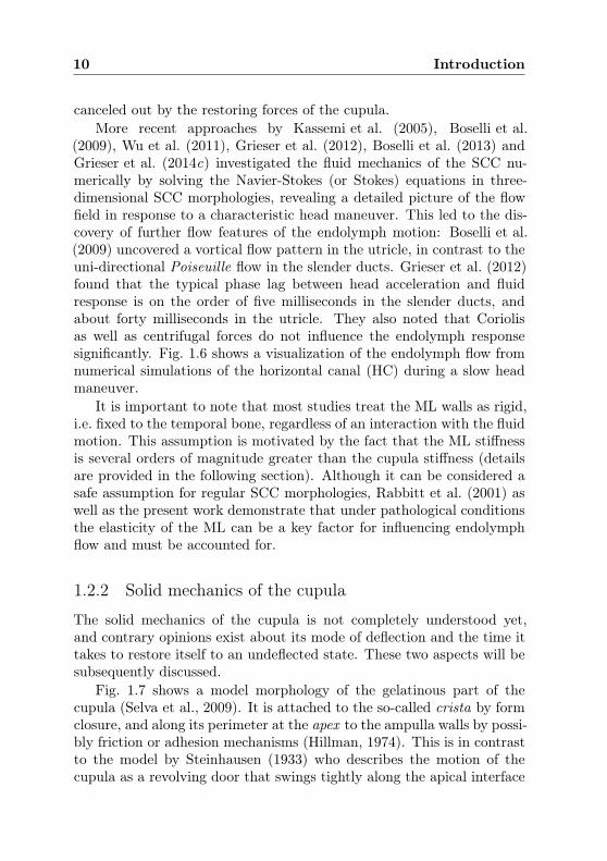
The solid mechanics of the cupula is not completely understood yet,and contrary opinions exist about its mode of deflection and the time ittakes to restore itself to an undeflected state. These two aspects will besubsequently discussed.

Fig. 1.7 shows a model morphology of the gelatinous part of thecupula (Selva et al., 2009). It is attached to the so-called crista by formclosure, and along its perimeter at the apex to the ampulla walls by possi-bly friction or adhesion mechanisms (Hillman, 1974). This is in contrastto the model by Steinhausen (1933) who describes the motion of thecupula as a revolving door that swings tightly along the apical interface

1.2 Mechanics of the vestibular system 11

at the ampulla walls. Later, Hillman & McLaren (1979) observed in bull-frogs that the cupula actually can detach at the apex due to excessiveendolymph movements. However, he remarks that this may more likelybe a relief mechanism to prevent destruction, and the physiological modeof oscillation resembles more that of a drum membrane.

This so-called sealed diaphragm hypothesis was then confirmed byRabbitt et al. (2009). They observed in oyster toadfishes that the cupuladetached itself from the apex only if the transcupular pressure reachedexcessive values (by un-physiological means of ML indentation), but nor-mally stays ‘attached around its entire perimeter’. Although the liter-ature has been discordant on the modes of deflection, it is commonlystated that there is no endolymph flowing past the moving cupula, en-dorsing a volume-displacement approach for the mathematical descrip-tion of cupula deflections.

)

crista

apex

Figure 1.7: Model morphology with characteristic dimensions of the human cupula.Adapted from Fig. 5a in Selva et al. (2009) with permission from IOS press and P.Selva.

A second controversy about the cupula characteristics is the timeconstant τc with which a physiological deformation decays back to theidle state. As a transcupular pressure builds up, the cupula deflectsand accumulates endolymph volume which gives rise to counter-actingstresses within the structure. Stiffer structures will exert stronger forcesfor the same displaced volume and thus result in a quicker, exponentialcupula recovery. Hence the cupula time constant correlates inverselywith the volumetric cupula stiffness, henceforth denoted by Kc.

Various studies have been performed on Kc and τc during the lastdecades, and their outcome offers quite a range of values: Jones et al.(1964) and Guedry et al. (1971) measure the time constant in humansto be 16 s (HC) and 7.2 s (PC, SC), while Dai et al. (1999) report it tobe 4.2 s on average (ten samples) using a model-based technique. The

12 Introduction

latter value was used by Obrist (2008) to derive a volumetric stiffness of13GPa/m3.

Figure 1.8: Superior canal dehiscence: schematic visualization of thepathoanatomy. Part of the temporal bone along the roof of the supe-rior canal is dehiscent and opens up to the dura mater (shown in blue)which covers the cranial cavity. Retrieved on January 12, 2015, fromhttp://www.earsite.com/what-is-superior-canal-dehiscence.

1.3 Superior canal dehiscence

The superior canal dehiscence (SCD) syndrome is a pathological condi-tion of the inner ear which remained unidentified until Minor et al. (1998)connected it to vestibular symptoms in response to sound and pressurestimuli. It refers to an abnormal absence or disruption of the tempo-ral bone which separates the inner-ear fluids from the cranial cavity, cf.Fig. 1.8. Predominantly affected due to its protuberant position withinthe temporal bone is the superior canal (SC), although dehiscences ofhorizontal (HC) and, even less likely, posterior canals (PC) have been re-ported as well (Chien et al., 2011; Cremer et al., 2000a; Erdogan et al.,2011; Krombach et al., 2006).

Section 1.3.1 gives a detailed description of the SCD pathophysiology,along with diagnostic and therapeutic measures to identify and poten-tially cure SCD patients. The so-called third-window theory is intro-duced in Section 1.3.2 and draws a connection to the fluid and solidmechanics of the semicircular canals (SCC), based on which a separatediscussion on the influence of the SCD on the stapes motility follows inSection 1.3.3.

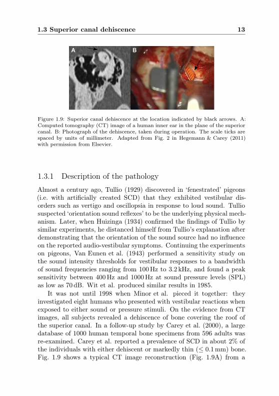
1.3 Superior canal dehiscence 13

Figure 1.9: Superior canal dehiscence at the location indicated by black arrows. A:Computed tomography (CT) image of a human inner ear in the plane of the superiorcanal. B: Photograph of the dehiscence, taken during operation. The scale ticks arespaced by units of millimeter. Adapted from Fig. 2 in Hegemann & Carey (2011)with permission from Elsevier.

1.3.1 Description of the pathology

Almost a century ago, Tullio (1929) discovered in ‘fenestrated’ pigeons(i.e. with artificially created SCD) that they exhibited vestibular dis-orders such as vertigo and oscillopsia in response to loud sound. Tulliosuspected ‘orientation sound reflexes’ to be the underlying physical mech-anism. Later, when Huizinga (1934) confirmed the findings of Tullio bysimilar experiments, he distanced himself from Tullio’s explanation afterdemonstrating that the orientation of the sound source had no influenceon the reported audio-vestibular symptoms. Continuing the experimentson pigeons, Van Eunen et al. (1943) performed a sensitivity study onthe sound intensity thresholds for vestibular responses to a bandwidthof sound frequencies ranging from 100Hz to 3.2 kHz, and found a peaksensitivity between 400Hz and 1000Hz at sound pressure levels (SPL)as low as 70 dB. Wit et al. produced similar results in 1985.

It was not until 1998 when Minor et al. pieced it together: theyinvestigated eight humans who presented with vestibular reactions whenexposed to either sound or pressure stimuli. On the evidence from CTimages, all subjects revealed a dehiscence of bone covering the roof ofthe superior canal. In a follow-up study by Carey et al. (2000), a largedatabase of 1000 human temporal bone specimens from 596 adults wasre-examined. Carey et al. reported a prevalence of SCD in about 2% ofthe individuals with either dehiscent or markedly thin (≤ 0.1mm) bone.Fig. 1.9 shows a typical CT image reconstruction (Fig. 1.9A) from a

14 Introduction

patient with superior canal dehiscence, along with a photograph (Fig.1.9B) taken during surgical repair.

Causes

The causes of SCD are highly debated and of multi-variate nature, asthe condition may either be inherited or acquired (Hegemann & Carey,2011). Among the etiologies of SCD are developmental abnormalitieswhich arise during childhood and usually affect both ears, as the tem-poral bone undergoes postnatal growth (Hirvonen et al., 2003). If a pre-disposition towards thin-walled SC roofs exists, it may erode over timedue to stresses from the ageing dura mater (visualized in blue, Fig. 1.8),or rupture as a consequence of accidental head trauma (Carey et al.,2000). Chien et al. (2011) lists other factors such as congenital defectsor chronic otitis media with cholesteatoma, the latter usually in conjunc-tion with horizontal canal dehiscences (Jang & Merchant, 1997).

Symptoms

According to Chien et al. (2011), typical symptoms of SCD patients in-volve sound-induced vertigo (Tullio phenomenon), pressure-induced ver-tigo (Hennebert Sign, Valsalva maneuvers), auditory hearing loss andbone conduction hyperacusis, as highlighted in the following. Symptomsinvolving vertigo are usually accompanied by saccadic eye movements(nystagmus) with a slow, upward-torsional component that correspondsto the affected canal plane (Minor, 2000).

Cases of the Tullio phenomenon (Tullio, 1929) often report triggerevents such as the loud and low-frequent sound of a toilet flush, or thenoise from a nearby screaming child. The vestibular response usuallypersists as long as the disturbing sound is emitted, and then tails offwithin seconds.

The Hennebert sign (Hennebert, 1911) classifies dizziness resultingfrom the application of pressure to the middle ear. Similar effects alongwith eye movements are observed when Valsalva maneuvers are per-formed, i.e. pressure applied against pinched nostrils or a closed glot-tis, as these increase the pressure in the middle ear or cranial cavity,respectively.

On top of their vestibular dysfunctions, patients further suffer fromauditory hearing loss in the dehiscent ear. When these patients areinvestigated by pure-tone audiometry, one typically finds an increase of

1.3 Superior canal dehiscence 15

air conduction thresholds in the affected ear (Kaski et al., 2012; Minor,2005).

Another side-effect of SCD is the hypersensitivity to bone-conductedsounds (bone conduction hyperacusis), with patients complaining abouthearing their own eyes move (Albuquerque & Bronstein, 2004) or otherbody sounds from their footsteps or voice (Hegemann & Carey, 2011).

Diagnosis

A series of diagnostic measures is required to distinguish SCD fromother pathologies in a patient with similar subsets of symptoms, such asMenière’s disease, Benign Paroxysmal Positional Vertigo (BPPV), Oto-

sclerosis of the middle ear, migraine-associated vertigo or labyrinthine

fistulae. In order to detect SCD during differential diagnosis, the follow-ing three procedures have become the gold standard.

A

B

Figure 1.10: Characteristic upward-torsional eye motion related to the Tullio phe-nomenon (TP) in patients with superior canal dehiscence (SCD) during exposure tosound (sound source in blue) in the affected ear (displayed in red).

A quick way to test for SCD is to investigate if the Tullio phenomenon(TP) is present. The eye motion is qualitatively observed during acousticstimulation by pure tones of elevated sound pressure level (approximately100dB SPL). Both ears are stimulated sequentially and at different fre-quencies through the unilateral application of an earphone. If TP occursduring exposure to sound waves in the affected ear, both eyes will reactby performing a slow, upward-torsional motion, followed by quick, sac-cadic reset movements (nystagmus). During torsion, the superior poleof the eyes moves ‘away’ (cf. Fig. 1.10) from the stimulated, affected ear,corresponding to an ampullofugal (excitatory) motion of the superiorcupula (Minor, 2000).

16 Introduction

More recently, also recordings of vestibular-evoked myogenic poten-tials (VEMP) have been used to diagnose a canal dehiscence by mea-suring the activity of ocular or cervical muscles. These responsescould be linked to vestibular activities of the utricle and saccule(Welgampola & Carey, 2010), ruling out potential cochlear origins. De-tails on this novel approach can as well be found in Brantberg et al.(1999).

Indispensable to a comprehensive diagnosis of SCD is the reconstruc-tion of computed tomography (CT) images of the inner ear in the planeof the superior canal (cf. Fig. 1.9A). As the dehiscence usually stretchesout to less than five millimeters, ultra-high-resolution CT scans are nec-essary to clearly identify the roof of the SC.

Treatment strategies

SCD patients currently face two different options for treatment: Bothcases usually follow the so-called middle fossa approach during whichthe superior surface of the temporal bone is surgically accessed. Thefirst option is to plug the SC completely, which results in a definiteloss of vestibular function in the vertical plane of the superior canal. Asecond procedure tries to maintain the SC functionality by resurfacingthe impaired bone. Although the latter approach seems more attractive,it is sided with a high relapse rate (Minor, 2005).

1.3.2 Third-window theory

Minor (2000) put forward the hypothesis that a dehiscence ‘creates athird mobile window into the inner ear’, and paved the way for the so-called third-window theory which has its origins in the early work byHuizinga (1934) and has not been refuted to this day. According to thetheory, the perilymph moves due to the presence of the third windowand leads to a cupula deflection within the respective canal. Carey et al.(2000) further specify the hypothesis by stating that the dehiscence al-lows ‘dissipation of the pressure as the membranous labyrinth bulgesinto the adjacent dura and endolymph flows away from the ampulla’.Carey et al. (2004) later add the possibility that ‘endolymph moves alonga path or multiple paths between the stapes and the dehiscence’, andthey hence suspect a shearing of the vestibular receptor organs along thetrajectory, ultimately resulting in nystagmus. However, they also notethat ‘the mechanisms by which acoustic stimuli act on the vestibular end

1.3 Superior canal dehiscence 17

organs are unclear’, and ‘may differ from the damped endolymph motionassociated with head acceleration’.

When Carey et al. (2004) measured firing rates of vestibular affer-ents in fenestrated chinchillas, they found that these animals would re-spond to loud sound with two types of mechanisms: irregular afferentswould phase-lock to the rapid stimulus below sound frequencies of 250Hz,whereas regular afferents generally underwent a slow, tonic increase infiring rate, up to a certain threshold. In one case of low frequency at125Hz, a regular HC afferent showed inhibitory behaviour, correspond-ing to a reversed, ampullopetal motion of the cupula. The regular af-ferents responded at sound intensities of 120 ± 8 dB, and the irregularafferents significantly lower at 92 ± 16 dB SPL. It is important to notethat although the dehiscence was created by Carey et al. on top of theSC, both SC and HC afferents would respond in the described patterns.It may be remarked here that the ampullae of SC and HC are adjacententities and linked by a short endolymph pathway via the utricle, cf. Fig.1.4.

Based on their findings, Carey et al. (2004) proposed two mechanismswhich could potentially explain the third-window hypothesis. First, anexcitation-inhibition asymmetry in the oscillatory EL motion (phasic re-sponse pattern of the irregular afferents) might lead to a net flow compo-nent (tonic response pattern of the regular afferents). Second, an organpipe analogy with resonance phenomena might explain the flow reversalat low frequencies.

1.3.3 Stapes motility effects on the perilymph

In the context of the SCD pathology, the frequency-dependent stapesmotility is of great importance as it determines the amplitude of theperilymph velocities (cf. Chapter 3.1), based on principles of momentumand mass conservation. In the following, we will first review the literatureon the frequency-sensitivity of stapes deflection velocities without SCD,and then complement them with a study that accounts for a dehiscence.

Frequency-sensitivity without SCD

Kringlebotn & Gundersen (1985) experimented with human cadavericears in order to assess the frequency characteristics of the middle ear.They found a peak sensitivity of round-window volume displacementsto sounds at around 1 kHz, with an exponential decay towards higher

18 Introduction

frequencies. Although Kringlebotn & Gundersen stated that ‘the trans-fer function of the middle ear cannot be measured in living humans’,Huber et al. (2001) succeeded in measuring the stapes velocity in liv-ing humans intra-operatively for the first time in humans using Laser-Doppler interferometry. When comparing their results to cadaveric mea-surements, they could not find a significant difference. This was recentlyconfirmed in similar experiments by Chien et al. (2009).

Figure 1.11 shows the transfer function of the middle ear, as measuredduring experiments on different species (living and dead), relating thestapes velocity to the incoming sound pressure level as a function ofthe sound frequency. For convenience, in the present work this transferfunction will be interchangeably referred to as ‘stapes motility’.

0

1

2

3

104

ChinchillaCat

Human cadaveric

Gerbil

Guinea pig

Human live corrected

+/- 95% CI

Human live uncorrected

Sta

pes

vel

oci

tyUs/ps

[

µm s/Pa]

Frequency f [kHz]

104

103

102

101

100

0.1 1 10

Figure 1.11: Comparison of normalized stapes velocity magnitudes Us/ps(f) fromdifferent species. Data labeled ‘Human cadaveric’ are from Kringlebotn & Gundersen(1985) and were edited by Chien et al. (2009). Data labeled ‘Human live corrected’and ‘Human live uncorrected’ are from Chien et al. (2009). Stapes velocities arenormalized by acoustic pressures ps. Adapted from Fig. 10 in Chien et al. (2009)who modified it from Fig. 8 in Rosowski et al. (1999). Reprint with permission fromElsevier and Karger.

Frequency-sensitivity with SCD

Kim et al. (2013) recently published numerical results from a finite ele-ment model of the middle and inner ear in the presence of SCD. They fo-cussed on the cochlear fluid pressures and the basilar membrane motion,as they were interested in quantifying the hearing loss in SCD patients.

1.4 Objectives and Outline 19

��1 1 10

��1

1

Frequency (kHz)

Frac

tio n

rd/r

SC=0.01

rd/r

SC=0.1

rd/r

SC=1

zero pressure

1

φ[-]

0.10.1 1 10

Frequency f [kHz]

rd/rSC=0.01rd/rSC=0.1rd/rSC=1zero pressure

Figure 1.12: Fraction φ(f) (‘cochlear admittance’) of the stapes-induced perilymphvolume displacement flowing into the cochlea for different ratios of dehiscence andcanal radii, D ≡ rd/rSC, as well as for a ‘zero pressure’ boundary condition at thelocation of the dehiscence. Adapted from Fig. A3 in Kim et al. (2013) with permissionfrom Elsevier.

The dehiscence was modeled by a Dirichlet-type pressure boundary con-dition, being a commonly used assumption (Obrist, 2011) to representthe reservoir character of the cerebrospinal fluid volume behind the sep-arating dura mater.

Kim et al. (2013) also determined the fraction of the stapes-inducedperilymph volume displacement which enters the cochlea and deflectsthe round window membrane (Fig. 1.12). In accordance with the third-window theory, the remaining perilymph displacement flows into thevestibular pathway(s). With these results at hand, one may deducethat the stapes induces perilymph oscillations which increasingly tend toprefer the vestibular pathways for decreasing frequencies. However, withregard to the measurements by Kringlebotn & Gundersen (1985), thestapes motility exerts the opposite behaviour for frequencies below 1 kHz(Fig. 1.11): the lower the frequency, the lower the stapes amplitudes. Theresulting pathological perilymph motion may hence comprise these twocounteracting mechanisms.

1.4 Objectives and Outline

The third-window theory of Minor (2000), along with first theoreticalconsiderations on the Tullio mechanism by Carey et al. (2004), offers aninterdisciplinary interface for research from an engineering perspective.To date, the remaining puzzle about the key mechanisms behind theTullio phenomenon has not been solved.

Current clinical treatments focus on restoring the roof of the dehis-

20 Introduction

cent canal, a surgical intervention with many risks. What if less invasivecures could be devised by means of changing the underlying mechanismto the favour of the patient? When its key parameters are revealed,would it not be tempting to see if slight changes in them could alleviatethe patient’s symptoms?

Numerical studies with a suitable computational model offer theunique chance to do so relatively easily, and sensitivity studies may beperformed at the expense of computer resources and to the benefit of the(unscathed) patient. Motivated by the prospect of an impact on humanhealthcare, this work pursues to identify the mechanism behind the su-perior canal dehiscence syndrome with a combined fluid-dynamical andmechanical approach.

Based on the ideas that were recently developed at the Institute ofFluid Dynamics (IFD) at ETH Zurich (Obrist, 2011), a novel hypothesisis formulated in Chapter 2 which tries to address the fluid-dynamical im-plications of the Tullio phenomenon. It involves nonlinear mechanismsof fluid-structure interaction in a strongly coupled environment of com-ponents with similar densities: endolymph, membranous labyrinth, andperilymph.

As the frequency spectrum of the coupled system spans three ordersof magnitude, Chapter 3 aims at devising a thorough modeling con-cept to render the complex reality with adequate simplifications. Thespatio-temporal modeling of the inner-ear physics intrinsically affectsthe feasibility of a numerical simulation with regard to its convergencebehaviour. In Chapter 4, we lay out our approach to discretize theidealized morphology and the model equations both in time and space,using state-of-the-art numerical methods which will be implemented ina tailor-made code.

With all tools at hand, numerical simulations are carried out and doc-umented in Chapter 5, upon which a discussion of the central aspectsfollows. By means of lumped-parameter models from prior investigationsof the author, the numerical results may then be brought into an appli-cable context of clinical relevance, connecting endolymph physics to thecharacteristic eye response patterns.

This thesis closes with concluding remarks on its findings in Chapter3.2.4, and gives an outlook on how to tap its full potential in follow-upstudies.

Parts of this work have been documented in Grieser et al. (2012) as

1.4 Objectives and Outline 21

well as in conference proceedings: Obrist et al. (2012)1, Grieser et al.(2014b)2, Grieser et al. (2014a)3, and Grieser et al. (2014c)3. Ourlumped-parameter modeling in Chapter 3 is based partly on the resultsin Grieser et al. (2014c).

19th European Fluid Mechanics Conference (EFMC-9), Rome285th GAMM Annual Meeting, Erlangen328th Bárány Society Meeting, Buenos Aires

Chapter 2

Hypothesis

The two sensory organs of the inner ear share the same fluid spaces ofperilymph (PL) and endolymph (EL) which are separated by the elasticwalls of the membranous labyrinth (ML). It seems surprising that we cansense motion and hear sound at the same time, given that both actionsinvolve motions of these fluids. Obviously there occur two different typesof fluid responses which (usually) do not interact.

10−2 Hz 100 Hz 102 Hz 104 Hz

100 s 1 s 10ms 0.1ms

hearing

balance

infrasound ultrasound

mechanical adaptation viscous blocking of inertial forces

Healthy adult

HSmechanical adaptation mechanical stimulation limit

TPweak nonlinearities strong damping

Patient with SCD

BCHno body motions no body motions

Figure 2.1: Temporal scale separation between hearing and balance in healthy adults,adapted from Fig. 20.1 in Obrist (2011) and supplemented with patho-physiologicalphenomena from patients with superior canal dehiscence (SCD): Tullio phenomenon(TP) from sound, Hennebert sign (HS) from pressure stimuli and bone conductionhyperacusis (BCH) to body sounds. Mechanisms of vestibular and cochlear originare shaded in green and gray, respectively.

From studies of the vestibular system (Chapter 1.2.1) we know thatthe endolymph is responsible for balance perception, and that it reacts tohead maneuvers only within a certain frequency range. If the maneuversare faster than about 10Hz, its inertial forces on the endolymph areinferior to the counter-acting viscous forces, and thus the endolymphdoes not respond. At slow maneuvers of less than 0.1Hz, the restoringforces of the cupula suppress a significant endolymph motion.

24 Hypothesis

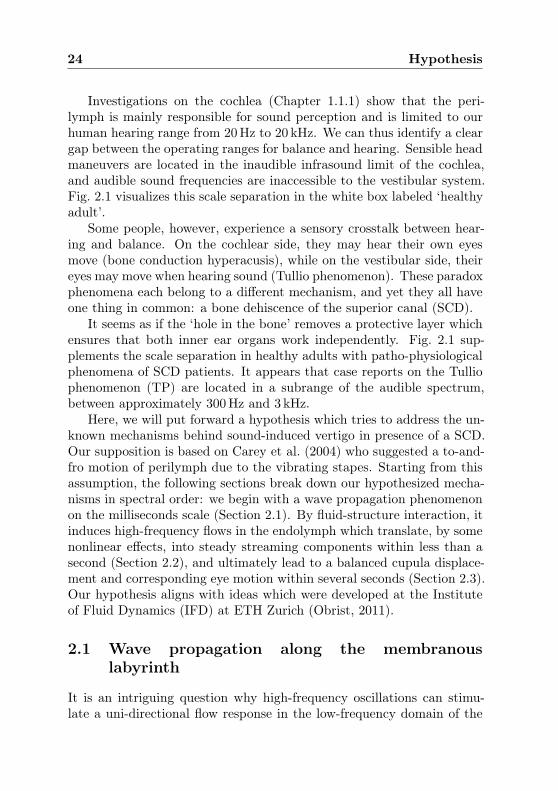
Investigations on the cochlea (Chapter 1.1.1) show that the peri-lymph is mainly responsible for sound perception and is limited to ourhuman hearing range from 20Hz to 20 kHz. We can thus identify a cleargap between the operating ranges for balance and hearing. Sensible headmaneuvers are located in the inaudible infrasound limit of the cochlea,and audible sound frequencies are inaccessible to the vestibular system.Fig. 2.1 visualizes this scale separation in the white box labeled ‘healthyadult’.

Some people, however, experience a sensory crosstalk between hear-ing and balance. On the cochlear side, they may hear their own eyesmove (bone conduction hyperacusis), while on the vestibular side, theireyes may move when hearing sound (Tullio phenomenon). These paradoxphenomena each belong to a different mechanism, and yet they all haveone thing in common: a bone dehiscence of the superior canal (SCD).

It seems as if the ‘hole in the bone’ removes a protective layer whichensures that both inner ear organs work independently. Fig. 2.1 sup-plements the scale separation in healthy adults with patho-physiologicalphenomena of SCD patients. It appears that case reports on the Tulliophenomenon (TP) are located in a subrange of the audible spectrum,between approximately 300Hz and 3 kHz.

Here, we will put forward a hypothesis which tries to address the un-known mechanisms behind sound-induced vertigo in presence of a SCD.Our supposition is based on Carey et al. (2004) who suggested a to-and-fro motion of perilymph due to the vibrating stapes. Starting from thisassumption, the following sections break down our hypothesized mecha-nisms in spectral order: we begin with a wave propagation phenomenonon the milliseconds scale (Section 2.1). By fluid-structure interaction, itinduces high-frequency flows in the endolymph which translate, by somenonlinear effects, into steady streaming components within less than asecond (Section 2.2), and ultimately lead to a balanced cupula displace-ment and corresponding eye motion within several seconds (Section 2.3).Our hypothesis aligns with ideas which were developed at the Instituteof Fluid Dynamics (IFD) at ETH Zurich (Obrist, 2011).

2.1 Wave propagation along the membranous

labyrinth

It is an intriguing question why high-frequency oscillations can stimu-late a uni-directional flow response in the low-frequency domain of the

2.1 Wave propagation along the membranous labyrinth 25

temporalbone

utricle

dehiscence

cupula

stapes

PL

ELcreflected

cincoming

ML

➂➁

➁➀

➀

➂

➀

➀

➀

➂

Figure 2.2: Visualization of the hypothesis: wave propagation of membrane displace-ments between stapes and dehiscence in the coupled system of perilymph (PL), mem-branous labyrinth (ML) and endolymph (EL). Double-sided arrows indicate the direc-tions of primary stapes/PL oscillations ➀, secondary ML deflections ➁, and tertiaryEL/cupula oscillations ➂. Membrane deflections travel with wavespeed c (red arrows)towards the dehiscence and get partly reflected at the same speed.

balance sense, simply by adding another ‘mobile window’ to the system.As different mechanisms may be at play, we start with an analysis of theinvolved components.

The vestibular pathway between the stapes and the dehiscence con-sists of two incompressible fluids (EL, PL) and their separating wall ofthe ML. Apart from the most direct path across the ampulla of the su-perior canal, also other perilymph pathways are conceivably actuated bythe stapes motion. However, since the flow resistance increases with thepath length, we expect that these do not contribute qualitatively to theresulting lymph flow induced by the dehiscence. As the ML is a sup-ple structure, its elasticity results in a finite wavespeed of the excited,coupled system by means of fluid-structure interaction (FSI). Similarsystems of FSI have been studied by Moens (1878) and Korteweg (1878),well-known by their findings on the combined wavespeed in elastic pipes,the so-called Moens-Korteweg wavespeed.

We assume that the compliant walls of the ML are subject to trans-mural pressure differences which originate from the stapes-induced per-ilymph oscillations. The transmural loads locally deflect the ML andprovoke a flow response of the endolymph and perilymph in its vicinity.

26 Hypothesis

As the overall volume of the inner-ear fluids stays constant, these flowswill be compensated by an inverse ML deflection in the near surroundings.This process repeats itself, thereby alternatingly creating displacementminima and maxima which meander along the ML towards the bone de-hiscence, with a finite propagation speed which is exclusively determinedby material and geometrical properties.

At the same time, the propagating deflections are attenuated alongtheir path by the damping nature of the fluid viscosity, such that theyare greatest in the vicinity of the stapes and smallest near the dehiscence.By equalizing the perilymph pressure to the pressure within the cranialcavity, the dehiscence can reflect part of the incoming wave train ofmembrane deflections, possibly creating interference patterns.

Inside the ‘rhythmically massaged hose’ of the ML, the endolymphis forced to flow back and forth at sound periods, pushing and drawingfluid into and from the utricle and thereby invoking corresponding de-flections of the cupula. We assume that these oscillations are causing thephase-locking behaviour of irregular cupula afferents which was reportedby Carey et al. (2004). Fig. 2.2 visualizes our hypothesis on the wavepropagation along the ML.

2.2 Steady endolymph streaming

It has been observed in similar studies on the basilar membrane of thecochlea that there are two nonlinear mechanisms at play which are ableto create a non-zero static component in an oscillatory flow: acousticstreaming due to Reynolds stresses (Lighthill, 1992) and steady stream-ing from FSI nonlinearities in the vicinity of vibrating walls (Edom et al.,2014).

We hypothesize that the endolymph flow which results from travelingwaves of radially oscillating ML walls shows an analogous behaviour, i.e.that it features both a static and a dynamic component. Furthermore,the strength and direction of the resulting net flow (steady streaming)may depend on the attenuation of traveling waves. These will be weaklyattenuated at low sound frequencies, yet strongly at high frequencies.

As the traveling waves get partly reflected at the location of thedehiscence and at the end of the canal, they can lead to interferencepatterns of nodes and anti-nodes if weakly attenuated. Such a scenariocan occur in a frequency range where the wavelength reaches the lengthscales of the canal. These waves are most likely incapable of generating

2.3 Cupula response 27

steady streaming, as the energy is ‘trapped’ between the interferencenodes. More importantly, Reynolds stresses in the fluid are generallyweaker at these lower frequencies.

In the other extreme, i.e. at high frequencies, strongly attenuatedwaves will ‘die out’ before they displace a significant part of the ML.Between these frequency limits, traveling waves may form. The soundspectrum in which the Tullio phenomenon occurs might be related tothese limits (cf. Fig. 2.1).

2.3 Cupula response

The cupula follows the pulsating endolymph flow such that it bulgesback and forth at sound periods, yet also continuously builds up a uni-directional displacement volume due to the static flow components. Aslong as the sound source persists to excite the stapes, a constant stream-ing force will act on the endolymph, thereby feeding a transcupularpressure difference. With increasing cupula deflection volume, restor-ing mechanical forces will counteract the motion such that less net flowis generated.

Eventually, a balance is reached where no additional streaming canbe produced as the restoring forces are as large as the streaming forces.At that point, the cupula maintains a constant deflection volume whichoscillates with zero mean mass flux. Due to the vestibulo-ocular reflex,a constant cupula displacement results in a constant slow-phase eye ve-locity. This process may explain the tonic behaviour observed in regularcupula afferents (Carey et al., 2004).

As soon as the sound stimuli disappear, the cupula moves back expo-nentially to its resting state, and likewise the slow-phase eye velocitiesin the vertical and torsional planes decay.

Although clinical data on the Tullio phenomenon report eye responseslargely corresponding to an ampullofugal deflection of the cupula, thereexist few cases of ampullopetal deflections. Such a flow reversal of thenet streaming may be explained by a frequency-dependent dominance ofeither the acoustic or the FSI-induced streaming mechanism which canoppose each other. It might also be associated with a shift in the windowlocation towards the common crus, such that the perilymph pathway tothe dehiscence gets redirected to oscillate primarily about the utricleinstead.

Chapter 3

Physical Modeling

An adequate physical model for a complex and heterogeneous systemsuch as the inner ear requires a clear definition of the effects which themodel should be capable of capturing.

According to the hypothesis in Chapter 2, nonlinear phenomena inthe endolymph as well as nonlinearities in the fluid-structure couplingmay be responsible for the evolution of steady endolymph streaming tocause sound-induced vertigo. As nonlinearities need to be linearized innumerical solution procedures, costly coupling algorithms are requiredto ensure convergence. The primary focus of our modeling efforts isto retain as much complexity as necessary in the model for the en-dolymph, and to simplify the remaining elements (perilymph, membra-nous labyrinth) of the coupled system as much as possible.

Keeping the numerical implications in mind, Section 3.1 seeks toformulate a physical model which is able to reflect the key features ofthe vestibular pathway between the stapes and the dehiscence. Basedon this modeling concept, the governing equations are derived for eachsubsystem in Section 3.2. Since we plan to perform a sensitivity studyon the Tullio phenomenon at a later stage, a dimensional analysis iscarried out in Section 3.3 from which we expect to gain insight into thesystem characteristics. According to the Buckingham Π theorem, e.g.as in Hornung (2006), a reduced set of dimensionless parameters can bederived which may greatly decrease the computational effort of our study.

Parts of this modeling approach were published in the form of conferenceproceedings in Grieser et al. (2014b).

3.1 Model formulation

In order to prove the existence of the hypothesized mechanical effectsof sound on the dehiscent vestibular organ, it may be sufficient to fo-cus exclusively on pure-tone acoustic stimulations for a relevant rangeof frequencies. If the suspected effect can be demonstrated by simple

30 Physical Modeling

Figure 3.1: Left : Physical model for sound-induced vertigo due to a dehiscence ofbone above the superior canal (SC) in the vestibular system. Upper right : Straight-ened model of the SC with concentric, circular cross-sections of endolymph (EL) andperilymph (PL), confined between the ampulla and the utricle, and separated bythe elastic membranous labyrinth (ML). Center right: Fluid-structure interactionbetween the one-dimensionally modeled PL/ML and the axisymmetric model of theEL. Lower right: Volume-based cupula model.

harmonics, it will most likely be present in more complex acoustic wave-forms, too. Therefore the stapes motion is modeled as a perfect sinusoid,well-defined by its amplitude (velocity Us) and the sound frequency f .

As the stapes vibrates, at least two oscillating fluid columns formin the perilymph (density ρf): one leads towards the round window viathe cochlear scalae, and the other(s) towards the dehiscence along thesemicircular canals (SCC).

Our physical model will only consider the shortest vestibular pathwaywhose centerline coordinate is denoted by x. It passes first the ampulla(x = 0) of the superior canal (SC) and then leads directly to the de-hiscence along the narrow duct (Fig. 3.1). The frequency-dependentadmittance φ of the cochlea in presence of an SCD is considered bypredictions from Kim et al. (2013), cf. Fig. 1.12. Apart from that, wedo not expect further implications on the balance sense which originatefrom the cochlear pathway.

We assume that the effects of the dehiscence on the stapes motility

3.1 Model formulation 31

can be neglected. Therefore we may obtain the vestibular perilymphflux simply by subtracting the cochlear share φ from the total, stapes-induced flux. This leads to vestibular perilymph velocity amplitudes Up

of

Up(f, SPL) = (1− φ(f)) · As

Ap· Us

ps(f) · ps(SPL) , (3.1)

where we take into account the lever arm between the stapes footplatearea As and the perilymph lumen Ap. Us/ps denotes the normalizedstapes velocity amplitudes. These can be measured in healthy adultswhich are subject to harmonic sound of acoustic pressure ps,

ps = pref · 10SPL20dB , (3.2)

defined by the sound pressure level (SPL) in logarithmic units of decibel(dB), which is related to a reference pressure of pref = 2 · 10−5 Pa (au-ditory threshold). An example for the lumped lever arm model (3.1) isgiven in Fig. 3.2.

100 1000 10 0000.01

0.1

1

10

100

1000

f [Hz]

Up/ps

[

µm s/Pa]

Figure 3.2: Perilymph velocity magnitudes Up in the dehiscent superior canal (SC),normalized by the acoustic pressure ps. Data plotted according to (3.1), with astapes footplate area and perilymph lumen of As = 3.21mm2 (Aibara et al., 2001)and Ap = 0.93mm2 (Curthoys et al., 1977), respectively. The normalized stapesvelocity amplitudes Us/ps(f) correspond to data labeled ‘Human cadaveric’ in Fig.1.11. The cochlear fluid fraction φ(f) corresponds to data labeled ‘zero pressure’ inFig. 1.12.

As we focus on purely sinusoidal stapes oscillations, we may assumethat the perilymph pulsates likewise at the ‘inlet’ of the SC, with angular

32 Physical Modeling

frequency ω = 2πf and velocity amplitude Up from (3.1). The perilymphvelocity and acceleration at the inlet boundary then become

up|0 (t) = Up cos(ωt) , (3.3a)

∂up

∂t

∣∣∣∣0

(t) = −Up ω sin(ωt) . (3.3b)

The excitation of the perilymph by the stapes can then be modeled bya time-dependent Neumann pressure boundary condition, i.e.

∂pp∂x

∣∣∣∣0

!= g(t) , (3.4)

with g(t) being a function of the perilymph velocity (3.3). It will bederived by a momentum analysis in Section 3.2.1.

At the location of the dehiscence (x= L1), the perilymph pressurepp is equal to the pressure in the cranial cavity across the dura mater,a supple structure of low impedance. We idealize this behaviour by aDirichlet boundary condition and set the reference pressure level at thedehiscence to zero at all times, i.e.

pp|L1

!= 0 . (3.5)

As the perilymph motion does not stop abruptly at the dehiscence, wealso consider the remaining (‘passive’) arm of the SC which goes pastthe SCD. Like the ‘active’ arm, it features a zero-pressure boundarycondition at the dehiscence. At the vestibule (x=L2), we set an outflowboundary condition, i.e.

∂pp∂x

∣∣∣∣L2

!= 0 (3.6)

From a modeling point of view, the passive arm of the SC can be un-derstood as a ‘better boundary condition’ on the active pathway. Bothpartitions are modeled as one-dimensional in x.

The canal’s major radius of curvature R is an order of magnitudegreater than the minor radius r0, i.e. R ≫ r0. Hence we neglect theinfluence of curvature and straighten the semicircular toroid to a perfectcylinder instead, as displayed in the upper right panel of Fig. 3.1.

The axisymmetric endolymph (density ρf , kinematic viscosity νf) con-sumes a concentric subspace of the SC. In contrast to the partitioned

3.1 Model formulation 33

perilymph, the endolymph consists of only one computational domainwith boundaries at the ampulla at x=0 and at the utricle at x=L2. Itfeatures an interface to the membranous labyrinth (ML).

Beyond its model boundaries, the endolymph is contained withinthe larger chambers of the ampulla (x < 0) and utricle (x > L2) whichcould be regarded as reservoirs into which it can be drawn or fed from.We reflect this reservoir character by an outflow boundary conditionwith vanishing velocity gradient in centerline direction (nx) and set thereservoir pressure to zero at all times, i.e.

(nx · ∇ue)x|0 = (nx · ∇ue)x|L2

!=0 , (3.7)

pe|0 = pe|L2

!=0 . (3.8)

We employ a linear-elastic (Young’s modulus E, Poisson ratio νs), one-dimensional (in x) and infinitely thin (virtual thickness h, density ρs)shell model for the ML along its interface between endolymph and peri-lymph. Since nonlinearities in the structure are neither expected to havea significant effect on the endolymph motion nor computationally justifi-able, they do not contribute to our model. The membrane displacementsη are treated as purely radial deflections (3.9) from their resting state atradius r0 due to transmural pressure differences ∆ps. The panel at thecenter right of Fig. 3.1 displays the described setup and introduces thenomenclature for this radial displacement as

r(x, t) = r0 + η(x, t) . (3.9)

As the total cross-section in the SC does not change in time due to therigid walls of the temporal bone, a local expansion of the perilymph areaAp will yield a corresponding contraction of the circular endolymph areaAe = r2π. Hence we obtain the following expressions using an indexnotation for the differentiation with respect to space and time variables,

∂Ap

∂x= −∂Ae

∂x= −2πrηx , (3.10a)

∂Ap

∂t= −∂Ae

∂t= −2πrηt , (3.10b)

∂2Ap

∂t2= −2πrηtt − 2πη2t . (3.10c)

The ratio of the areas at the resting state (index ‘0’) will be referred to

34 Physical Modeling

as ‘perilymph dominance’ and is defined as

β ≡ Ap,0

r20π. (3.11)

Fluid-structure interactions take place at the ML interface (index ‘Γ’).We follow a so-called ‘Dirichlet-Neumann’ approach (cf. Chapter 4.3)which sub-iterates for the membrane displacements (Dirichlet conditionon the fluid velocity boundary) and the corresponding fluid pressure atthe walls (Neumann condition on the structure boundary), i.e.

nΓ · ue,Γ!= ηt , (3.12)

∆ps!= pe|Γ − pp . (3.13)

The cupula model is displayed in the lower left panel of Fig. 3.1 and isbased on the commonly used volume approach (displacement volumeVc) which was explained in Chapter 1.2.2. The model requires a stiffnessparameter Kc to relate volumetric deflections to transcupular pressures.Since the cupula motion due to the elastic restoring forces is threeorders of magnitude slower than the high-frequency fluid oscillations,they will exclusively be applied on the mean streaming motion in aseparate model (cf. Section 3.2.4).

A schematic overview of our modeling approach is given by the blockdiagram in Fig. 3.3.

3.2 Governing equations

As the physical model is now clearly defined along the boundaries of itssubspaces, the governing equations are laid out in the order of their phe-nomenological appearance: we begin with a derivation of the perilymphequations in Section 3.2.1. In Section 3.2.2, we formulate the equationof motion for the elastic membrane and combine it monolithically withthe fluid mechanics of the perilymph. Section 3.2.3 introduces the en-dolymph equations. Since the modeled cupula response builds up on thetemporal mean of the endolymph flow (steady streaming), we establisha connection to the vestibulo-ocular reflex in Section 3.2.4.

3.2.1 Perilymph

The one-dimensionally modeled perilymph varies along its centerline inarea Ap, pressure pp, and velocity up. We can postulate the principle of

3.2 Governing equations 35

f

φSPLUsps

E Up

Ue

Vc

αt

Cochlear flux pred.(Fig. 1.12)

Stapes motility meas.(Fig. 1.11)

Lumped lever arm model(Eq. 3.1)

Analyticalfit from

sensitivitystudies

(Eq. 5.24)

Numericalsimulation

of vestibularsystem

Cupula mechanics(Eq. 3.35)

VOR electro-mech.(Eq. 3.36)

As

Ap

L1

L2

r0hβρfρsνfνs

K1,...,K5

Kc

ρfνfL2

r0

Kα

Figure 3.3: Block diagram displaying the transfer function circuit to model sound-induced vertigo in patients with SCD. Input/output variables (encircled): soundfrequency f , sound pressure level (SPL), cochlear fluid fraction φ, stapes motilityUs/ps, perilymph velocity amplitude Up, membrane Young’s modulus E, steady en-dolymph streaming Ue, cupula displacement volume Vc, eye velocity αt. All othersymbols denote system constants corresponding to the (patho-)anatomy of an indi-vidual patient. Center box : an analytical fit of Ue becomes available after numericalsensitivity studies in the patho-physiological range of interest (E, f , Up).

36 Physical Modeling

mass conservation, i.e.

∂Ap

∂t+

∂(Apup)

∂x= 0 , (3.14)

which may be expanded and rewritten to arrive at an expression for thespatial velocity gradient,

∂up

∂x= − 1

Ap

∂Ap

∂t− up

Ap

∂Ap

∂x. (3.15)

By differentiating (3.15) with respect to time, we obtain

up,xt = − 1

Ap

∂2Ap

∂t2+

1

A2p

(∂Ap

∂t

)2

− ∂

∂t

(up

Ap

∂Ap

∂x

)

. (3.16)

We can further postulate conservation of momentum in the peri-lymph, i.e.

∂ (Apup)

∂t+ ǫp (Apup) = −Ap

ρf

∂pp∂x

, (3.17)

with a pseudo-viscous damping ǫp to account for the radial effects ofthe viscous term which a one-dimensional model cannot resolve. It canbe shown (Appendix A) that in flows of high Womersley numbers, i.e.strongly pulsating flows where transient forces dominate over viscousforces, the pseudo-viscous damping becomes

ǫp ≈ ω = 2πf . (3.18)

We expand and rewrite (3.17) such that we obtain

∂up

∂t= − 1

ρf

∂pp∂x

− ǫpup − up

Ap

∂Ap

∂t. (3.19)

This expression can further be differentiated with respect to the axialcoordinate, i.e.

up,tx = − 1

ρf

∂2pp∂x2

− ǫp∂up

∂x− ∂

∂x

(up

Ap

∂Ap

∂t

)

, (3.20)

and by substituting the spatial velocity gradient on the right-hand sidewith (3.15), we get

up,tx = − 1

ρf

∂2pp∂x2

+ǫpAp

∂Ap

∂t+ǫp

(up

Ap

∂Ap

∂x

)

− ∂

∂x

(up

Ap

∂Ap

∂t

)

. (3.21)

3.2 Governing equations 37

When we subtract (3.21) from (3.16), the velocity derivatives drop outand the pressure gradient of second order can be obtained by rearrangingthe expression as follows,

1

ρf

∂2pp∂x2

=1

Ap

∂2Ap

∂t2+

ǫpAp

∂Ap

∂t− 1

A2p

(∂Ap

∂t

)2

+

+

(∂

∂t+ ǫp

)

·(up

Ap

∂Ap

∂x

)

− ∂

∂x

(up

Ap

∂Ap

∂t

)

(3.22)

Appendix B demonstrates that (3.22) can further be simplified using(3.10), (3.15) and (3.19). The result comprises three terms of increasingnonlinearity on the right-hand side, and reads

∂2pp∂x2

= −2πρfr

Ap(ηtt + ǫpηt)− 2πρf

1

Apη2t + 2π

1

Ap

∂pp∂x

ηx . (3.23)

As it is a priori unclear whether the higher order terms in (3.23) play asignificant role in the generation of the hypothesized endolymph stream-ing, we kept them in our set of equations. However, it may be remarkedhere that an a posteriori assessment of (3.23) by means of numericalsimulations revealed that the last two terms are smaller than the othersby at least two orders of magnitude. We found also that the geometricalratio r/Ap could safely be approximated by its value at the resting state,r0/Ap,0. Substituting (3.11), a purely linear relationship follows whichyields equivalent results as (3.23), i.e.

∂2pp∂x2

≈ − 2ρfβr0

(ηtt + ǫpηt) . (3.24)

We will continue the description of our modeling with the linearizedexpression in (3.24). For the sake of completeness, however, theneglected nonlinear terms will reappear in dimensionless form (3.55)at the end of the present chapter. The effect of these terms will bequantified in Chapter 5.2.3.

Since two boundary conditions are specified for each partition of theperilymph in (3.4)-(3.6), the pressure can be calculated by integrating(3.24) twice with respect to the axial coordinate x. The active andpassive arms are denoted by ‘I’ and ‘II’, respectively, and one obtains

I : pp(x, t) = −L1∫

x

x∫

0

∂2pp∂x2

d˜x dx− (L1−x) · g(t) , (3.25a)

38 Physical Modeling

II : pp(x, t) = −x∫

L1

L2∫

x

∂2pp∂x2

d˜x dx . (3.25b)

In the following, we derive the stapes boundary condition g(t) onthe perilymph. Using the momentum balance in (3.17), we solve for thespatial gradient of the perilymph pressure, i.e.

∂pp∂x

= −ρf∂up

∂t− ǫpρfup − ρfup

Ap

∂Ap

∂t. (3.26)

By substituting Ap,t with (3.10b), the last term on the right-hand sideof (3.26) can be rewritten as

−ρfup

Ap

∂Ap

∂t=

2πr

Apηtρfup . (3.27)

The radial membrane velocity ηt has an approximate amplitude of|ηt| ≈ ηmax · ω, with a maximal membrane displacement of ηmax ≪ r.Expanding the fraction in (3.27) with the tube radius r and substitutingthe angular frequency ω with (3.18), we obtain

∣∣∣∣

2πr

Apηtρfup

∣∣∣∣≤(

2Ae

Ap︸︷︷︸

<1

ηmax

r︸ ︷︷ ︸

≪1

)

· ωρf |up| ≪ ǫpρf |up| , (3.28)

which shows that the third term on the right-hand side of (3.26) is sig-nificantly smaller than the second term and may be safely neglected.With the perilymph velocity from (3.3a) and its temporal derivativefrom (3.3b), we arrive at a definition for the Neumann boundary condi-tion g(t), i.e.

g(t) ≈ −ρf∂up

∂t

∣∣∣∣0

− ǫpρf up|0 = ρfUp (ω sin(ωt)− ǫp cos(ωt)) . (3.29)

3.2.2 Membranous labyrinth

Gautier et al. (2007) derived the governing equations for an axisymmet-ric, elastic membrane which is subject to transmural pressure differencescaused by its surrounding fluids. Their equations consider axial and ra-dial membrane motions, and account for possible axial preloads as well

3.2 Governing equations 39

as variations in the Poisson ratio νs. According to Gautier et al., thereexist five different types of waves which arise in such a coupled system offluid-structure interaction (FSI). Four of them ‘mainly propagate withinthe structure: the torsional shell wave [...], a quasi-longitudinal wave[...], (and) longitudinal/flexural waves’. The only wave which is stronglycoupled to the fluid motion is found to be the ‘quasi-plane acoustic wave’related to the theory of Korteweg (1878).

As we are mainly interested in the fluid response, we consider onlythese quasi-plane acoustic waves which do not require an axial couplingwithin the structure. Therefore we may simplify the governing equa-tions from Gautier et al. (2007) by omitting axial motions and axialpreloads, and arrive at a linear, one-dimensional model of masses andradial springs,

ρshηtt +Eh

r20 (1− ν2s )η = ∆ps = pe,Γ − pp . (3.30)

With the perilymph pressure pp given by (3.25) and its second derivativepp,tt from (3.24), the membrane model in (3.30) can be partitioned (I, II)and rewritten as

I :

ρsh+2ρfβr0

L1∫

x

x∫

0

( · ) d˜xdx

ηtt +

ǫp2ρfβr0

L1∫

x

x∫

0

( · ) d˜xdx

ηt

+

Ehs

r20 (1− ν2s )

η = pe,Γ + (L1−x)g(t) , (3.31a)

II :

ρsh+2ρfβr0

x∫

L1

L2∫

x

( · ) d˜xdx

ηtt +

ǫp2ρfβr0

x∫

L1

L2∫

x

( · ) d˜xdx

ηt

+

Ehs

r20 (1− ν2s )

η = pe,Γ . (3.31b)

Evidently, in (3.31) the perilymph adds damping characteristics to themembrane motion, as well as it increases the effective mass of the oscilla-tory system. Introducing mass (Cm), damper (Cd) and spring coefficients(Cs) as the respective bracketed expressions in (3.31), and denoting theright-hand side with d, the membrane dynamics may be reformulated as

40 Physical Modeling

a system of first-order differential equations, i.e.[Cm Cd0 1

][ηtη

]

t

=

[0 −Cs1 0

][ηtη

]

+

[d(x, t)

0

]

. (3.32)

3.2.3 Endolymph

The endolymph motion is governed by the Navier-Stokes equations inan axisymmetric coordinate system. These comprise the conservation ofmass and momentum,

∇ · ue = 0 , (3.33a)∂ue

∂t+∇ · (ueue) = − 1

ρf∇pe + νf∇ · (∇ue) . (3.33b)

Bold symbols denote vectorial quantities of axial (x) and radial (r) com-ponents. The momentum equation (3.33b) will not be simplified, as wewant to capture the nonlinear effects which lead to steady endolymphstreaming. Like the perilymph, the endolymph is a viscous fluid thathas a similar density (ρf) and kinematic viscosity (νf) as water.

3.2.4 Cupula and vestibulo-ocular reflex

In the present section we are only concerned with the mean flow (steadystreaming Ue) of the oscillating endolymph.

Before the onset of a net cupula deflection, at time t= t0, a trans-cupular pressure ∆pc builds up as nonlinear mechanisms force the en-dolymph in a certain direction (cf. Section 2.3). Drag forces counteractthe fluid motion, and we may obtain the pressure gradient along the canalby assuming Poiseuille flow. It leads to the so-called Hagen-Poiseuille

equation,

∆pc(t0) = −L2∫

0

∂pe∂x

∣∣∣∣SC

dx ≈ 8ρfνfr20

Ue

L2∫

0

dx =8ρfνfL2

r20Ue . (3.34)

With increasing net cupula displacement volume Vc, the transcupularpressure yields restoring forces until a balance is obtained in which noadditional streaming can be generated from the stimulus. At that time(t = t∞), the cupula has reached a constant deflection volume,

Vc(t∞) =1

Kc∆pc(t0) =

8ρfνfL2

Kcr20Ue(t0) . (3.35)

3.3 Dimensional analysis 41

Grieser et al. (2014c) studied the endolymph and cupula dynamics ina three-dimensional morphology of the horizontal canal (HC) in re-sponse to patient-specific video head impulse tests (vHIT). Numericalsimulations of the cupula displacement volume Vc were compared withmeasured eye velocities αt. Their model featured a cupula stiffness ofKc = 600GPa/m3 which was calibrated such that the simulated expo-nential decay as exp(−t/τc) was in accordance with the literature, i.e.τc ≈ 4.4 s.

Revisiting these results in the context of the present work, we iden-tified a proportionality constant Kα = 122 ◦s−1/0.003mm3, relating αt

and Vc. Assuming that the superior canal (SC) has similar characteris-tics, we may incorporate these findings into our model and obtain

αt|V/T(t∞) ≈ KαVc(t∞) =8KαρfνfL2

Kcr20Ue(t0) ≡ KsUe(t0) , (3.36)

for vertical (V) and torsional (T) velocity components of the eye motion.By linear superposition principles, we could hence show that the

sound-induced eye velocity is proportional to a steady endolymph stream-ing at the onset of the sound stimulus. With typical values for the geo-metrical and material properties, i.e.

ρf = 103 kgm−3, νf = 10−6 ms−1, L2 = 9mm, and r0 = 160µm ,

this proportionality constant becomes approximately Ks ≈ 191◦/mm.A vertical/torsional eye velocity of 19◦/s would thus correspond to asteady endolymph streaming of around 0.1mm/s.

3.3 Dimensional analysis

The governing equations for the coupled motion of perilymph and mem-brane in (3.31) as well as for the endolymph in (3.33) were derived indimensional form. In the following, we carry out a dimensional analysisto determine the reduced set of dimensionless parameters which com-pletely define our system.

Substituting the pseudo-viscous damping ǫp with the angular fre-quency ω due to (3.18), we identify eleven dimensional quantities ofcombinations of three different SI units, listed in Tab. 3.1. Accordingto the Buckingham Π theorem (cf. Hornung (2006)), there exist exactly

42 Physical Modeling

Symbol Description System SI Unitsω Sound frequency PL s−1

Up Velocity amplitude PL ms−1

Ap,0 Cross-sectional area PL m2

L1 Dehiscence location PL mL2 SCC length PL/ML/EL mr0 Radius PL/ML/EL mh Thickness ML mE Young’s modulus ML kgm−1 s−2

ρs Density ML kgm−3

ρf Density PL/EL kgm−3

νf Viscosity EL m2 s−1

Table 3.1: Eleven dimensional quantities which completely define the physical modelof perilymph (PL), membranous labyrinth (ML) and endolymph (EL).

eight (11−3= 8) independent, dimensionless parameters. As these canbe arbitrarily recombined to a different but equivalent set of eight pa-rameters, one tries to choose them such that they comprise already well-established numbers. Our choices are listed below.

Korteweg number Ko ≡

√Eh

ρf2r0r0

νf(3.37)

Fluid loading L ≡ ρf2r0ρsh

(3.38)

Reynolds number Re ≡ Upr0νf

(3.39)

Womersley number Wo ≡ r0√

ωνf

(3.40)

Perilymph dominance β ≡ Ap,0

r20π(3.41)

Density ratio γ ≡ ρsρf

(3.42)

Location of the dehiscence κ1 ≡ L1

r0(3.43)

Length of the SCC κ2 ≡ L2

r0(3.44)

It may be noted that the ‘perilymph dominance’ β was already intro-

3.3 Dimensional analysis 43

duced in (3.11) and has been reproduced by the dimensional analysis.The so-called ‘fluid loading’ L was mentioned by Gautier et al. (2007) intheir study of elastic tubes undergoing FSI. We further assign a ‘Korte-weg number’ Ko which may be understood as a Reynolds number whosecharacteristic velocity is given by the Korteweg wave speed cK,

cK =

√

Eh

ρf2r0, Korteweg (1878). (3.45)

In the following, we eliminate the dimensional variables from our setof equations. Dimensionless coordinates and flow variables are distin-guished from their dimensional couterpart by a prime (′), as given below.

x′ ≡ 1

r0· x (3.46)

t′ ≡ ω · t (3.47)

η′ ≡ 2

r0· η (3.48)

p′e ≡1

ρf (r0 ω)2· pe (3.49)

p′p ≡ 1

ρf (r0 ω)2· pp (3.50)

u′e ≡

1

r0 ω· ue (3.51)

From these definitions, we can also derive the differentiated quantitieswhich appear in the governing equations, i.e.

∇′ = r0 · ∇ , ∇′2 = r20 · ∇2 ,

η′t =2

r0 ω· ηt , η′tt =

2

r0 ω2· ηtt ,

η′x = 2 · ηx ,

p′p,x =1

ρf r0 ω2· pp,x ,

u′e,t =

1

r0 ω2· ue,t .

Based on the dimensionless parameters defined by (3.37)-(3.44) and the

44 Physical Modeling

non-dimensionalized variables from (3.46)-(3.51), we can recast our set ofequations. The active arm of the coupled perilymph-membrane systemis defined between 0≤x′≤κ1 and then becomes

I :1

L η′tt +Ko2

Wo4 (1− ν2s )η′ +

1

β

κ1∫

x′

x′

∫

0

(η′tt + η′t) d˜x′dx′

= p′eΓ +Re

Wo2(κ1 − x′)(sin t′ − cos t′) . (3.52)

Likewise, the passive arm is defined between κ1 ≤ x′ ≤ κ2 and can bereformulated as

II :1

Lη′tt+Ko2

Wo4(1− ν2s )η′+

1

β

x′

∫

κ1

κ2∫

x′

(η′tt + η′t) d˜x′dx′ = p′eΓ . (3.53)

Finally, the dimensionless Navier-Stokes equations may be obtained.They describe the motion of the endolymph between 0 ≤ x′ ≤ κ2, i.e.

∇′ · u′e =0 (3.54a)

u′e,t +∇′ · (u′

eu′e)−

1

Wo2∇′2u′

e =−∇′p′e . (3.54b)

For the sake of completeness, we may also derive the non-dimensionalizedequation for the active arm which includes all higher order terms, givenby

I :1

Lη′tt+Ko2

Wo4(1− ν2s )η′+

1

β

κ1∫

x′

x′

∫

0

(η′tt+η′t)1 + 1

2η′

1− 1β η

′− 14β η

′2d˜x′dx′

+1

β

κ1∫

x′

x′

∫

0

η′2t

12

1− 1β η

′− 14β η

′2d˜x′dx′

− 1

β

κ1∫

x′

x′

∫

0

p′p,xη′x

1 + 12η

′

1− 1β η

′− 14β η

′2d˜x′dx′

= p′eΓ+Re

Wo2(κ1−x′)(sin t′−cos t′) .

(3.55)

3.3 Dimensional analysis 45

The influence of the higher order terms in (3.55) on the steady endolymphstreaming will be assessed and quantified in Chapter 5.2.3.

Chapter 4

Numerical Modeling

The present chapter lays out the numerical discretization approachwhich we apply to our physical model. The computational domainis discretized in Section 4.1. We identify two sub-systems: the one-dimensional system of the perilymph, coupled to the membranouslabyrinth, and the three-dimensional axisymmetric endolymph domain.These are highlighted separately in Section 4.2 with regard to the spatial

and temporal discretization of their governing equations. The densitiesof the fluids are similar to the density of the membranous labyrinth,such that we deal with a strongly coupled problem (Causin et al.,2005). A coupling algorithm is devised in Section 4.3 to synchronize thesolution variables along the common interface. The performance of thefluid-structure coupling is analysed in Chapter 4.4.

Parts of this chapter were documented in conference proceedings(Grieser et al., 2014b). The numerical model was implemented in atailor-made solver called tullioFoam, written in C++ language. The com-mented program code is electronically available (Grieser et al., 2015).

4.1 Discretization of the computational domain

Figure 4.1 illustrates the spatial discretization of our model. We split thecoupled, one-dimensional system of the perilymph and the membranouslabyrinth at the location of the dehiscence into the directly stimulated,‘active’ arm (I) and the indirectly excited, ‘passive’ arm (II). The domainsare discretized along the axial coordinate x into NI and NII equidistantvertices with mesh widths ∆xI and ∆xII, respectively. Each vertex rep-resents a computational node at which we solve for the radial membranedisplacements η and perilymph pressures pp. The node at x=L1 belongsto both domains. The length of the SCC, L2, corresponds to

L2 = (NI − 1) ·∆xI + (NII − 1) ·∆xII . (4.1)

In the computational domain of the endolymph, we do not distinguishbetween the active and the passive arm. The whole canal is discretized

48 Numerical Modeling

by an array of Nx×Nr hexahedral volumes, representing an axisymmetricwedge which revolves around the line of symmetry at r=0. The verticesat the corner are locked axially to the corresponding vertices of thecombined membrane-perilymph system. Endolymph pressures pe andvelocities ue are stored in the respective centers of the finite volumes.Initially, these are equally spaced in the radial direction with a meshwidth ∆r. In the course of the simulation, the corner vertices at themembrane interface Γ will follow the radial displacements η.

We evaluate and store the pressure and velocity boundary conditionsin the face centers of the membrane interface, pe,Γ and ue,Γ. As thecombined membrane-perilymph domain needs to access the endolymphpressure at the corner vertices, values of pe,Γ are interpolated from theface centers by bilinear schemes.

NI NII

∆xI

Nx

∆xII

∆r

Nr

0

r0

r

0 L1 L2

x

η, pp

pe,Γ

pe,ue

EL

ML & PL

Γ

‘active’ arm (I) ‘passive’ arm (II)

Figure 4.1: Numerical discretization of the computational domains of perilymph (PL),membranous labyrinth (ML) and endolymph (EL). At the dehiscence (x=L1), thecoupled, one-dimensional system of ML and PL is split into the ‘active’ (I) and‘passive’ (II) arms. Each arm is discretized by N equidistant (∆x) vertices (◦) whichrepresent the computational nodes for ML displacements η and PL pressures pp. Theaxisymmetric domain of the EL is discretized by an array of Nx ×Nr finite volumesin the axial and radial direction, respectively. Center points (•) store velocities ue

and pressures pe. Face centers (�) at the ML interface (Γ) store pressures at theboundary, pe,Γ. Vertices of the EL (◦) move in the radial direction, yet maintaintheir axial location (coupled to the ML).

4.2 Discretization of the governing equations 49

4.2 Discretization of the governing equations

In the following sections, the governing equations are discretized in thecoupled membrane-perilymph domain and the endolymph.

4.2.1 Coupled system of membrane and perilymph

We restate the system of first-order differential equations,[Cm Cd0 1

][ηtη

]

t

=

[0 −Cs1 0

][ηtη

]

+

[d(x, t)

0

]

. (3.32⋆)

In our spatial discretization approach, the membrane motion is eval-uated at N computational nodes. We obtain the solution vector,

e ≡[ηt

η

]

∈ IR(2N×1) . (4.2)

Likewise, the right-hand side vector of (3.32) is discretized as

q ≡[d0

]

∈ IR(2N×1) , (4.3a)

I : d = pe,Γ + g(t) (L1 1− x) , (4.3b)

II : d = pe,Γ . (4.3c)

Here, 0 and 1 denote a column vector of N zeros and ones, respectively.The mass, damper and spring coefficient matrices are given by

Cm = ρsh I +2ρfβr0

AB , (4.4a)

Cd = ǫp2ρfβr0

AB , (4.4b)

Cs =E h

r20 (1− ν2s )I , (4.4c)

with an identity matrix I and two spatial-integral matrices, A and B,

I : A =

∫ L1

x

(·)dx , B =

∫ x

0

(·)dx , (4.5a)

II : A =

∫ x

L1

(·)dx , B =

∫ L2

x

(·)dx . (4.5b)

50 Numerical Modeling

The numerical integration in axial direction uses a trapezoidal scheme,

xb∫

xa

( · )dx ≈ ∆x

2

b−1∑

i=a

[( · )i + ( · )i+1] , (4.6)

such that the integral operators become triangular matrices,

I : A =L1

2 (NI− 1)

1 2 2 · · · 2 2 10 1 2 · · · 2 2 1

0 0 1. . . 2 2 1

......

. . .. . .

. . ....

...

0 0 0. . . 1 2 1

0 0 0 · · · 0 1 10 0 0 · · · 0 0 0

∈ IR(NI×NI)+ , (4.7a)

B =L1

2 (NI− 1)

0 0 0 · · · 0 0 01 1 0 · · · 0 0 0

1 2 1. . . 0 0 0

......

. . .. . .

. . ....

...

1 2 2. . . 1 0 0

1 2 2 · · · 2 1 01 2 2 · · · 2 2 1

∈ IR(NI×NI)+ , (4.7b)

II : A =L2−L1

2 (NII− 1)

0 0 0 · · · 0 0 01 1 0 · · · 0 0 0

1 2 1. . . 0 0 0

......

. . .. . .

. . ....

...

1 2 2. . . 1 0 0

1 2 2 · · · 2 1 01 2 2 · · · 2 2 1

∈ IR(NII×NII)+ , (4.7c)

B =L2−L1

2 (NII− 1)

1 2 2 · · · 2 2 10 1 2 · · · 2 2 1

0 0 1. . . 2 2 1

......

. . .. . .

. . ....

...

0 0 0. . . 1 2 1

0 0 0 · · · 0 1 10 0 0 · · · 0 0 0

∈ IR(NII×NII)+ . (4.7d)

4.2 Discretization of the governing equations 51

We denote the (invertible) coefficient matrices by

M ≡[Cm Cd

0 I

]

∈ IR(2N×2N) , (4.8a)

N ≡[0 −Cs

I 0

]

∈ IR(2N×2N) , (4.8b)

such that we can write the discretized time derivative of the solutionvector in the simple form

et = M−1(

N e+ q)

. (4.9)

The temporal discretization is performed at discrete times tn+1 =tn +∆t with a constant timestep ∆t. We apply the generalized Crank-Nicolson method,

en+1−en

∆t= ϑen+1

t + (1−ϑ)ent , (4.10)

with a coefficient ϑ ∈ [0, 1]. The scheme is implicit unless ϑ=0 (Eulerforward scheme). The convergence tests in Section 4.4 are carried outin the range between ϑ=0.5 (Crank-Nicolson scheme) and ϑ=1 (Eulerbackward scheme). Applying (4.10) to (4.9) leads to

en+1−en

∆t= ϑM−1

(

N en+1 + qn+1)

+(1−ϑ)M−1(

N en + qn)

. (4.11)

Defining the (invertible) matrix G by

G ≡ I −∆t ϑM−1N , (4.12)

and introducing a coefficient matrix K with

K ≡ ∆tG−1M−1 , (4.13)

it can be shown that the discretized equation in (4.11) may be rewrittenwith respect to the solution increment ∆e,

∆en+1 ≡ en+1−en , (4.14)

52 Numerical Modeling

as

∆en+1 = K(

N en + ϑqn+1 + (1−ϑ)qn)

. (4.15)

Hence we are able to numerically determine the membrane motion attime tn+1 directly from the old state at time tn, given that we know theright-hand side q at time tn+1. Since the right-hand side depends on theendolymph pressure at the interface, pp,Γ, the coupling of the governingequations requires an implicit strategy (cf. Section 4.3).

The coupled membrane-perilymph equation (4.15) is implemented in oursolver tullioFoam. All matrix and vector operations as well as corre-sponding data input/output are carried out using the Armadillo library(Sanderson, 2010). Further details on tullioFoam will follow in the sub-sequent sections of the present chapter.

4.2.2 Endolymph

In Section 4.1 we discretized our computational domain for the en-dolymph into finite volumes. Without internal re-meshing, a movingboundary such as the membrane interface would lead to significant vari-ations of the cell volume in its vicinity. Such inhomogeneities may giverise to numerical errors and a smooth cell distribution is desirable at alltimes.

Therefore we apply a computationally inexpensive, algebraic ap-proach to re-mesh the grid: we restrict the vertex positions to radialrelocations, rv(xi), and we move them proportionally to the local bound-ary displacement η(xi) and their relative tube location rv/rΓ by

rn+1v (xi) = rnv +

rnvrnΓ

(ηn+1 − ηn

), i = 1, . . . , Nx+1 . (4.16)

An internal re-meshing has an arbitrary character, as it does not reflectphysical motions inside the domain. However, any change of the cellvolume results in numerical fluxes ϕg across the cell surface S which mustbe accounted for when we solve for physical fluxes ϕe. The ArbitraryLagrangian Eulerian (ALE) approach considers these by substitutingadvective fluxes with relative ones, ϕrel, defined by

ϕrel ≡ ϕe − ϕg =

∫

S

n · (ue − ug) dS , (4.17)

4.2 Discretization of the governing equations 53

where ug and n denote grid velocities and surface normals, respectively.

Furthermore, the space conservation law (Demirdžić & Perić, 1988) en-sures that a change in cell volume V is equal to the integral of the gridfluxes ϕg across the cell surface S,

d

dt

∫

V

dV =

∫

S

n · ug dS . (4.18)

Using (4.17)-(4.18), the Navier-Stokes equations (3.33) are integratedover the cell volume V according to the Finite-Volume Method (FVM).We obtain the well-known discretization in the ALE formulation,

∫

S

n · ue dS = 0 , (4.19a)

d

dt

∫

V

ue dV +

∫

S

n · (ue − ug)ue dS =

− 1

ρf

∫

S

n pe dS + νf

∫

S

n · (∇ue) dS , (4.19b)

where volume integrals over vector or scalar fields (◦/•, 4.20) were sub-stituted by surface integrals according to Gauss’ theorem or the Green-

Gauss theorem, respectively, given by∫

V

∇ · (◦) dV =

∫

S

n · (◦) dS , (4.20a)

∫

V

∇(•) dV =

∫

S

n (•) dS . (4.20b)

Details on the ALE approach can be found e.g. in Donea et al. (2004)and Duarte et al. (2004).

Our code tullioFoam solves (4.19) using the open source library ofOpenFOAM in the extended version, 1.6-ext. The fluid solver as well asthe treatment of the moving domain boundary Γ has been adapted froma solver1 by Ž. Tuković and P. Cardiff.

1icoFsiElasticNonLinULSolidFoam, available in OpenFOAM ‘foam-extend-3.1’

54 Numerical Modeling

Startj=0

Update mesh fluxes

Solve momentum eq.

PISO loopj++

Split operators

Solve Poisson eq.(N⊥ successive repeats)

Update velocity

j?= 2

End

Figure 4.2: Numerical simulation of the endolymph by a pressure-implicit algorithmwith splitting of operators (PISO), as implemented in OpenFOAM.

The solver follows the PISO algorithm (Issa et al., 1986), sketchedin Fig. 4.2. It consists of a momentum predictor step and a pressurecorrection loop. The momentum is predicted by solving (4.19b) for thevelocity ue based on old values for the pressure pp and the flux ϕe.When the divergence operator is applied on (4.19b), the transient andviscous terms vanish due to mass conservation. Splitting the operators ofthe nonlinear term, a Poisson equation can be obtained which is solvediteratively for the pressure.

For PISO, we use a preconditioned bi-conjugate gradient solver(PBiCG) with a diagonal incomplete-LU preconditioner (DILU) forthe iterative solution of the endolymph velocity during the momentumpredictor step. The pressure correction loop employs a generalizedgeometric-algebraic multi-grid solver (GAMG) with a Gauss-Seidelsmoother, and is repeated twice. In order to compensate for non-orthogonalities inside the mesh, the Poisson equation is successivelyrepeated N⊥ times before the momentum flux is corrected. Each

4.3 Fluid-structure coupling 55

Type Selected Scheme Accuracy OpenFOAM Keyword

Time deriv. Euler backward 2nd order backward

Divergence Central scheme 2nd order Gauss linear

Gradient Central scheme 2nd order Gauss linear

Laplacian Central scheme 2nd order Gauss linear corrected

Table 4.1: Selected spatial and temporal discretization schemes from the library ofOpenFOAM.

distribution of OpenFOAM already ships with our selected solutionschemes.

Tab. 4.1 lists the numerical schemes we selected for the discretizationof the respective operators in (4.19). A documentation of these schemesas well as of the software library in general can be retrieved online fromthe OpenFOAM Foundation (2015). Information on the FVM in movingmeshes can be obtained from Jasak & Tukovic (2004). Examples of FSIwith OpenFOAM are given in Jasak & Tukovic (2010).

4.3 Fluid-structure coupling

Three media are interacting with each other. Two of them, the perilymphand the membranous labyrinth, were combined and solved monolithically,as described in Section 4.2.1. Their solution variable η, however, dependson the endolymph pressure at the membrane interface, pe, and vice versa.This interdependence is even enhanced by the condition that the involvedmedia feature similar densities, rendering the need for a strongly iterativeprocedure to couple both subsystems (Causin et al., 2005).

Therefore, we apply the Dirichlet-Neumann approach (cf. Fig. 4.3)which has been suggested in similar studies on liquid-filled flexibletubes, e.g. by Causin et al. (2005), Küttler & Wall (2008), Nobile(2009), Astorino & Grandmont (2010), Fernández et al. (2010) andDegroote & Vierendeels (2011). Structural displacements (η) and ve-locities (ηt) are imposed on the boundaries of the fluid which returnsloads (pe,Γ) on the structure interface.

In order to obtain convergence during a timestep, the displacementsare typically relaxed towards the previous solution. Various relaxationschemes exist in the literature, ranging from simple relaxation constants,analysed in Causin et al. (2005), to dynamically adapting parameters

56 Numerical Modeling

Dirichlet

Neumann

η F(η,ηt)

peS(

pe,Γ)

Fluid-StructureCoupling

Figure 4.3: Partitioned Dirichlet-Neumann approach to couple the membrane motionη iteratively with the endolymph pressure pe at a given instant in time. F denotes thefluid solver, supplied with Dirichlet boundary conditions from the structure (imposeddisplacements and velocities). S denotes the solid solver, supplied with a Neumannboundary condition from the fluid (imposed loads).

such as in the IQN-ILS (interface-quasi-Newton with inverse Jacobianfrom a least-squares model) method by Degroote et al. (2009).

We apply the so-called Aitken relaxation according to a recursive pro-cedure described in Küttler & Wall (2008). During each iteration stepi, the Aitken parameter θ is dynamically recalculated from the historyof the solution residual resi. The Aitken method is embedded into oursolver framework as described in the following.

Fluid-structure coupling algorithm

Figure 4.4 displays a schematic overview of the fluid-structure couplingalgorithm as it is implemented in our numerical solver tullioFoam.

The stapes boundary condition g(tn+1) is evaluated at the beginningof each time step tn+1. For numerical reasons, the amplitude of g(t) isgradually increased from zero at the onset of the simulation (tn= t0) toits stationary maximum, given in (3.29), over a time span of at least fivewave periods. Details on the applied ramp function R can be found inAppendix C.

Before entering the Aitken loop, we provide initial guesses (i = 0) forthe solution variables by means of an extrapolation from previous times,i.e.

∆en+10 =∆en , (4.21)

4.3 Fluid-structure coupling 57

Startn=0

Create mesh

Initialize fields

Calculate matrices

Time loopn++

Update stapes boundary

Guess solution at i=0

Aitken loopi++

Update right-hand side

Solve membrane

Relax solution

Update mesh

Solve endolymph (PISO)

εA?< ε0A

εV?< ε0V

End

Figure 4.4: Solution algorithm for numerical simulations of the Tullio phenomenon,as implemented in our code tullioFoam. Fluid-structure coupling is performed usingthe Aitken relaxation.

58 Numerical Modeling

(pe,Γ

)n+10 =2(p

e,Γ)n − (p

e,Γ)n−1 . (4.22)

Within the Aitken loop, we calculate the right-hand side of the coupledmembrane-perilymph equation using (4.3),

qn+1i−1

= f(

(pe,Γ

)n+1i−1 , g(tn+1)

)

. (4.23)

A preliminary solution of the membrane motion is denoted by a tildeand may now be obtained by

∆en+1i = K

(

N en + ϑqn+1i−1

+ (1−ϑ)qn)

. (4.24)

With the displacement residual given by

resi ≡ ∆ηi−∆η

i−1, (4.25)

the Aitken relaxation parameter θ is calculated by the recursive definitionfrom Eq. 44 in Küttler & Wall (2008), i.e.

θi−1 = θ0 ∈ [0, 1] , i = 1 , (4.26a)

θi−1 = −θi−2

resi−1 ·(resi − resi−1

)

(resi − resi−1

)·(resi − resi−1

) , i > 1 . (4.26b)

Additionally, we limit the relaxation to values of

|θ| ≤ 1 . (4.27)

The preliminary solution is now relaxed by

∆en+1i = θi−1∆en+1

i + (1− θi−1)∆en+1i−1 , (4.28)

and the membrane motion e = [ηt, η]T can be obtained from

en+1i = en +∆en+1

i . (4.29)

The mesh vertices at the boundary are re-positioned according to the newmembrane displacement η, and the internal vertices of the endolymphdomain are redistributed according to the algebraic definition in (4.16).Additionally, we impose Dirichlet constraints on the velocity boundary

4.4 Convergence analysis 59

of the endolymph by assuming no-slip conditions along the membraneinterface Γ, i.e.

nΓ · ue,Γ!= ηt . (3.12⋆)

With the updated mesh at hand, we solve the Navier-Stokes equationsfor the endolymph, as described by the PISO algorithm in the previoussection. At the end of each Aitken cycle, a normalized residual εA iscomputed according to

εA ≡ 1

r0

√√√√ 1

N

N∑

v=1

res2(xv) , N = NI +NII − 1 . (4.30)

If the normalized residual falls below a pre-defined tolerance limit,

εA < ε0A , (4.31)

we exit the Aitken loop and advance in time by ∆t.

As we aim for a periodic steady-state solution during the continuousstimulation by the stapes, we introduce a convergence criterion to endthe time loop. As long as transient effects of either physical or numericalorigin persist, errors relating to the lack of periodicity (‘beat volumeerrors’) are recorded by comparing the total domain volume to previousperiods. Hence we define a normalized beat residual as

εV ≡

N∑

j=1

Vj(tn+1)−

N∑

j=1

Vj(tn+1 − T )

r20πL2, N = NxNr , (4.32)

where Vj is the annular cell volume of a cell with index j, obtained byrevolving the cell about the line of symmetry. A convergence limit wasspecified by

|εV| < ε0V . (4.33)

Selected tolerance levels are given in Tab. 4.2.

4.4 Convergence analysis

The convergence of tullioFoam is analyzed based on a default set ofparameters for our computational model, given in Tab. 4.3.

60 Numerical Modeling

ε0A ε0V ε0p ε0u

10−10 10−8 10−8 10−6

Table 4.2: Relative tolerance levels for Aitken relaxation, εA (4.30), beat volume error,εV (4.32), endolymph pressure residual, εp (Poisson eq.), and endolymph velocityresidual εu (momentum eq.). Values correspond to our solver settings.

Symbol Value Description

r0 160µm initial radius of membranous labyrinth

L1 5mm axial location of dehiscence

L2 9mm length of SCC

β 10 perilymph dominance (3.41)

h 20µm membrane thickness

ρs 1200 kg/m3 membrane density

νs 0.5 membrane Poisson ratio

νf 10−6 m2/s fluid viscosity

ρf 1000 kg/m3 fluid density

ϑ 0.6 generalized Crank-Nicolson scheme coefficient

θ0 1.0 initial Aitken relaxation

T/∆t 200 time steps per sound period

NI 400 no. of vertices in active arm

NII 320 no. of vertices in passive arm

Nr 32 no. of cells in radial direction

Table 4.3: Default parameter values of the computational setup.

Aitken loop

Figure 4.5 displays the observed convergence behavior of the Aitkenresidual εA. With the onset of a growing residual history at the sec-ond iteration step, the Aitken relaxation dynamically re-calibrates itself.Initially the coupling errors increase for two iteration steps. However,after the fourth iteration we observe a continuous decrease which decaysby a slope of

∂ (log10εA)

∂i≈ −0.13 , i > 12 . (4.34)

4.4 Convergence analysis 61

1 10 20 30

10−10

10−8

10−6

10−4

Aitken iteration i [-]

Aitken

resi

dualε A

[-]

εA (average)

ε0A=10−10

slope −0.13

Figure 4.5: Convergence of the Aitken residual εA (4.30) within 32.2 iteration steps onaverage at default model configuration (Tab. 4.3). Residuals are ensemble-averagedover all time steps, thus continuous in i. Circles indicate integer values of i. Thedashed line corresponds to the slope of the logarithmic residual decay. Aitken loopsare terminated if εA < ε0A.

Approaching the limits of numerical accuracy, the Aitken loop terminatesas soon as the residual drops below a value of ε0A = 10−10.

Time loop

Advancing in time, we seek to determine the state of periodic steadinessof our results, characterized by vanishing beat volume errors εV in thedeforming computational domain of the endolymph. When the stimula-tion by the stapes is smoothly ramped up to reach full load at t=5T , weobserve initial oscillations of the residual which are locked to the stim-ulus frequency (Fig. 4.6). These errors recede with ongoing simulationtime until they practically disappear at t = 10T . Furthermore we de-tect a second pulsation pattern of lower frequency fV, clearly visible att>10T . It possibly relates to the time it takes to propagate membranedeflections through twice the length of the canal (forth and back). Atthis point, we may estimate these volume pulsations fV by the Kortewegwave speed (3.45), and obtain

fV =cK2L2

, (4.35)

62 Numerical Modeling

0 5 10 20 30 40 50

10−10

10−8

10−6

10−4

10−2

L2

cK

Time t [T ]

Bea

tvolu

me

resi

dual|ε

V|[−

] εV > 0

εV < 0

ε0V=10−8

slope: −0.12

Figure 4.6: Convergence of the beat volume residual εV (4.32) during numericalsimulation at default model configuration (Tab. 4.3). Stapes amplitudes are broughtto full load (cf. Appendix C) during the first five sound periods T =1/f , visualized byvertical, dotted lines. Oscillating residual values are displayed by magnitudes, withsigns (+/-) indicated by different colors (black/grey). The dashed line correspondsto the slope of residual decay. A thick bar depicts the time which Korteweg wavesneed to reach the end of the canal, x=L2, at speed cK (3.45). Simulations terminateif |εV| < ε0V for at least three consecutive sound periods.

which is independent of the stapes vibration mode of frequency f . Simi-lar to the Aitken loop, we observe that the beat volume residual decaysby a slope of

∂ (log10εV)

∂(t/T )≈ −0.12 . (4.36)

When the residual reaches the limits of numerical accuracy, we terminatethe simulation as soon as it falls below a value of ε0V = 10−8 for at leastthree consecutive sound periods.

Total computation time

Fig. 4.7(a) shows how the choice of the generalized Crank-Nicolsonscheme coefficient ϑ affects the total simulation time to reach a peri-odic solution. We observe that an increase in ϑ towards the first-orderimplicit Euler backward scheme at ϑ=1 reduces the accuracy of a singleAitken iteration and thus requires more iteration steps to converge, cf.Fig. 4.7(b).

4.4 Convergence analysis 63

0.5 0.6 0.7 0.8 0.9 1.00

10

20

30

40

50

Generalized Crank-Nicolson scheme coefficient ϑ

Com

puta

tion

tim

e[hrs]

(a)

0.5 0.6 0.7 0.8 0.9 1.020

40

60

80

Generalized Crank-Nicolson scheme coefficient ϑ

Num

ber

ofev

ents

[−]

No. of sim. periods T

Av. no. of Aitken steps

(b)

Figure 4.7: Computational effort in numerical simulations with the solver tullioFoamto obtain a periodically steady state. Analysed for different values of the generalizedCrank-Nicolson scheme coefficient, ϑ ∈ [0.5, 1.0], visualized by circles1. (a) Totalcomputation time. (b) No. of simulated sound periods T and average no. of Aitkeniterations per time step. Dashed lines correspond to polynomial fits through the re-spective data. Simulations were carried out in nonparallel mode on desktop computerswith an Intel® Core™ i5 CPU 650 processor (3.2GHz, 8GB memory). Simulationsetup corresponds to default parameters listed in Tab. 4.3.

However, as we approach the lower limit corresponding to the second-order accurate Crank-Nicolson scheme at ϑ = 0.5, numerical dampinglessens. Therefore physical oscillations which arise from the gradualapplication of loads below t≤5T decay slower over time, resulting in anincrease in the overall run time.

These two counteracting mechanisms - numerical accuracy vs. numer-ical damping - lead to an optimum in computational efficiency which isroughly located at ϑ≈0.6, as the polynomial fit in Fig. 4.7(a) indicates.

1Data acquisition by Benner (2015)

Chapter 5

Results and Discussion

A numerical solution algorithm for fluid-structure interactions insidethe inner ear was devised and tested for convergence in Chapter 4. Us-ing the computational infrastructure at the Institute of Fluid Dynamics(IFD) at ETH Zurich, a series of numerical simulations have been carriedout with the tailor-made solver tullioFoam. The results of these simu-lations will be presented in Sections 5.1-5.3, and subsequently discussedin Section 5.4.

The findings are grouped in three parts: we begin with first-orderflow phenomena, i.e. the wave propagation of physical quantitiesbetween the oscillating stapes and the dehiscence (Section 5.1). Thisis followed by an evaluation of the second-order mean flow, as we seekto confirm the hypothesized steady endolymph streaming (Section 5.2).Using the principles of dimensional analysis, the underlying mechanismsmay be identified and formulated at that point. Section 5.3 puts theresults of the mean flow analysis into the context of clinical relevance.We will translate the calculated steady endolymph streaming via cupulamechanics and the VOR into slow-phase eye velocities of a virtual Tulliopatient, and compare these velocities to clinical data available in theliterature.

Preliminary results were documented in conference proceedings(Grieser et al., 2014a,b). Data acquisition and post-processing was inpart1,2 accomplished by Benner (2015) in the course of a Master thesisunder supervision of the author.

5.1 First-order flow: wave propagation

The wave propagation along the canal is successively analyzed by isolat-ing three major effects which determine the speed, the amplitude andthe attenuation of the waves. In Section 5.1.1, we investigate how the

1Data acquisition: Figs. 5.7-5.11, 5.20, 5.21, 5.242Post-processing: Figs. 5.20, 5.24

66 Results and Discussion

wave speed depends on the membrane stiffness. Section 5.1.2 focuses onthe effect of the stapes motility on wave amplitudes. In Section 5.1.3, wevary the sound frequency within the audible spectrum to detect changesin the wave attenuation.

5.1.1 Wave speed

In a first approximation, the wave speed in the coupled system of per-ilymph, membranous labyrinth and endolymph is solely determined bymaterial constants (membrane stiffness E, fluid density ρf) and cross-sectional dimensions (endolymph radius r0, membrane thickness h, peri-lymph lumen Ap). Most of these parameters are well documented in theliterature such that we can rely on values from anatomical measurements,e.g. by Curthoys & Oman (1987).

However, measurements of Young’s modulus E are extremelyrare, and were performed exclusively ex vivo or in animals, e.g. byYamamoto & Ishii (1991) and Rabbitt et al. (1999). Since the mem-brane properties may change significantly after death, we cannot resortto statistically firm values for the human membrane stiffness in our mod-eling. In theory, the whole range between the cupula stiffness of approx-imately 21Pa (McHenry & van Netten, 2007) to the stiffness of bone ofapproximately 18GPa (Fung, 1981) is possible, spanning across nine or-ders of magnitude. Practically, we may limit our sensitivity study to areasonable range between E > 1 kPa and E < 100 kPa, which coincideswith stiffness values of the adjacent cochlear membranes, as measuredby Gueta et al. (2011), for instance.

According to the theory by Korteweg (1878), we expect that the wavespeed is proportional to the square root of the membrane stiffness, as

cK =

√

E h

ρf 2r0. (3.45⋆)

Therefore, as we ‘scan’ through two orders of magnitude for the mem-brane stiffness, we can expect the realistic wave speed to differ from ourresults at most by one order of magnitude. Subsequently, we carriedout numerical simulations for different Young’s moduli E of the mem-brane. Figs. 5.1-5.2 show the periodic steady-state propagation of radialmembrane deflections η and velocities ηt which we obtained for differentYoung’s moduli at otherwise standard parameters (Tab. 4.3).

5.1 First-order flow: wave propagation 67

We observe that the wavelength λ increases as the membrane stiffens,which corresponds to an increase of the wave speed c since

c = λ · f . (5.1)

Additionally, we note that the oscillation amplitudes are two orders ofmagnitude smaller than the tube radius, i.e. η/r0 ≪ 1, and that theydecay towards the dehiscence. As the membrane stiffens, the amplitudesdecrease as expected.

The interface pressures of the perilymph, pp, and the endolymph,pe,Γ, are displayed in Figs. 5.3 and 5.4, respectively. We find that thepressure amplitudes increase with Young’s modulus. In contrast to theendolymph, the pressure in the perilymph is dominated by the stapesforcing and only slightly oscillates along the membrane, maintaining analmost constant spatial pressure gradient throughout the active pathwaybetween the stapes and the dehiscence. The endolymph pressure, on theother hand, shows a strongly oscillatory behavior with predominantlytraveling waves which decay towards the end of the canal.

Fig. 5.5 completes the picture with plots of the instantaneous en-dolymph velocities in the axial and radial directions. We identify equallyspaced spots of alternating flow reversals which correspond to the wave-length λ, consistent with the wavelengths of the membrane displacementη in Fig. 5.1. According to the no-slip constraint, the radial endolymphvelocities at the membrane interface are equal to the membrane veloci-ties from Fig. 5.2. We observe a phase shift of 90◦ with respect to theaxial velocity pattern.

The Korteweg theory can be extended to a more general descriptionof the acoustic wave propagation in elastic tubes, using a dispersion equa-tion (Gautier et al., 2007, Eq. 4, p. 335). The restriction to high fluidloadings L ≫ 1 was lifted, and variations in the Poisson ratio νs 6= 0 wereaccounted for. Furthermore, Gautier et al. captured interdependenciesfrom longitudinal waves within the structure, cL, and from the speed ofsound within the fluid, cf ≈1520m/s, such that the limitation

r20ω2 ≪ c2L ≪ c2f (5.2)

of the Korteweg theory could be overcome. An exact solution of the dis-persion equation for ‘unstretched’ membranes was given (Gautier et al.,2007, Eqs. 8-10, p. 337), which may be rewritten as

c1 = +(−)

√

2 c2La+

√b

, (Acoustic wave, radial oscillation) (5.3a)

68 Results and Discussion

x=0 L1 L2

−2

−1

0

1

2

Dis

pla

cem

entη[µm] envelope

η(t0)η(t0+1/8T )η(t0+2/8T )η(t0+3/8T )

(a) E = 5kPa

0 L1 L2

−2

−1

0

1

2

(b) E = 10 kPa

0 L1 L2

−2

−1

0

1

2

(c) E = 20 kPa

0 L1 L2

−2

−1

0

1

2

(d) E = 40 kPa

Figure 5.1: Wave propagation along the membranous labyrinth for different Young’smoduli E at sound frequency f = 400Hz, visualized by consecutive snapshots ofradial membrane displacements (gray shades) and the corresponding envelope(red).

5.1 First-order flow: wave propagation 69

x=0 L1 L2

−4

−2

0

2

4

Vel

oci

tyηt[m

m/s]

envelopeηt(t0)ηt(t0+1/8T )ηt(t0+2/8T )ηt(t0+3/8T )

(a) E = 5kPa

0 L1 L2

−4

−2

0

2

4

(b) E = 10 kPa

0 L1 L2

−4

−2

0

2

4

(c) E = 20 kPa

0 L1 L2

−4

−2

0

2

4

(d) E = 40 kPa

Figure 5.2: Wave propagation along the membranous labyrinth for different Young’smoduli E at sound frequency f = 400Hz, visualized by consecutive snapshots ofradial membrane velocities (gray shades) and the corresponding envelope (red).

70 Results and Discussion

x=0 L1 L2

−20

−10

0

10

20

Pre

ssure

pp[Pa]

envelopepp(t0)pp(t0+1/8T )pp(t0+2/8T )pp(t0+3/8T )

(a) E = 5kPa

0 L1 L2

−20

−10

0

10

20

(b) E = 10 kPa

0 L1 L2

−20

−10

0

10

20

(c) E = 20 kPa

0 L1 L2

−20

−10

0

10

20

(d) E = 40 kPa

Figure 5.3: Wave propagation along the membranous labyrinth for different Young’smoduli E at sound frequency f =400Hz, visualized by consecutive snapshots of theperilymph pressure (gray shades) and the corresponding envelope (red).

5.1 First-order flow: wave propagation 71

x=0 L1 L2

−20

−10

0

10

20

Pre

ssure

pe,Γ

[Pa]

envelopepe(t0)pe(t0+1/8T )pe(t0+2/8T )pe(t0+3/8T )

(a) E = 5kPa

0 L1 L2

−20

−10

0

10

20

(b) E = 10 kPa

0 L1 L2

−20

−10

0

10

20

(c) E = 20 kPa

0 L1 L2

−20

−10

0

10

20

(d) E = 40 kPa

Figure 5.4: Wave propagation along the membranous labyrinth for different Young’smoduli E at sound frequency f =400Hz, visualized by consecutive snapshots of theendolymph pressure (gray shades) and the corresponding envelope (red).

72 Results and Discussion

x=0 L1 L2

−r0

0

r0

Radia

lco

ord

inate

r 15

0

−15

5

0

−5

ux[m

m/s]

ur[m

m/s]

(a) E = 5kPa

0 L1 L2

−r0

0

r0

(b) E = 10 kPa

0 L1 L2

−r0

0

r0

(c) E = 20 kPa

0 L1 L2

−r0

0

r0

(d) E = 40 kPa

Figure 5.5: Wave propagation within the endolymph for different Young’s moduli Eat sound frequency f =400Hz, visualized by snapshots of axial (r > 0) and radial

endolymph velocities (r<0).

5.1 First-order flow: wave propagation 73

c2 = +(−)

√

2 c2La−

√b

, (Longitudinal wave, axial oscillation) (5.3b)

cL =

√

E

ρs (1− ν2s ), (5.3c)

a =L −

(

1− r20ω2

c2L

)

·(

1− c2Lc2f

)

− ν2s · c2Lc2f

(1− ν2s )− r20ω2

c2L

, (5.3d)

b = a2 − 4L −

(

1− r20ω2

c2L

)

· c2Lc2f

(1− ν2s )− r20ω2

c2L

. (5.3e)

Fig. 5.6 shows our simulation results for the combined wave speed c fordifferent Young’s moduli E and sound frequencies f , and compares themto the analytical predictions by Korteweg and Gautier et al.. It may beremarked that our results additionally contain compliance effects due tothe presence of the perilymph, which generally leads to reductions in thecombined wave speed c.

In the lower audible range, i.e. for f <500Hz, the simulation resultsalign well with the predictions by Korteweg (1878) within the investi-gated spectrum of Young’s moduli. As the sound frequency approachesthe ring frequency fπ (Gautier et al., 2007), i.e. associated with the timethat longitudinal waves need to travel around the circumference of themembrane,

fπ =cL

2πr0, (5.4)

such that r20ω2 ≪/ c2L, our numerical model deviates from the Korteweg

theory towards lower wave speeds, recovering the analytical referenceby Gautier et al.. The latter asymptotically decays to zero speed atf = fπ, corresponding to the onset of a ‘stop band’ for acoustic waves(Gautier et al., 2007), up to ultrasound in the inaudible MHz range.Since the Tullio phenomenon has been reported at sound frequenciesas high as 3 kHz (Cremer et al., 2000b), we are led to the conclusionthat the stop band must begin at higher frequencies. Hence Young’smodulus of the membranous labyrinth must be at least E>10 kPa (Fig.5.6(b)), as there would occur no wave propagation otherwise.

74 Results and Discussion

5.1.2 Wave amplitude

During stimulation by sound, the stapes vibrates sinusoidally with fre-quency f at amplitudes Us. As mentioned earlier, studies by Huber et al.(2001) and Chien et al. (2009) found that the amplitudes are not onlypatient-specific, but also vary greatly across the audible spectrum (cf.Chapter 1.3.3), and depend on the sound pressure level (SPL). It is ourintention to separate these anatomical boundary conditions from themechanism which generates wave propagations along the membranouslabyrinth. Apart from the sound frequency, our numerical model thusrequires only the specification of a perilymph velocity amplitude Up atx=0. This amplitude Up may be obtained separately and prior to thenumerical simulation, as sketched in Fig. 3.3.

In the present section, we investigate the effects of Up on the wavepropagation along the canal. For this purpose, we keep the soundfrequency and the membrane stiffness constant and vary Up within arealistic range of values. The results for η, ηt, pp, pe,Γ and ue are shownin Figs. 5.7-5.11, respectively.

We find that all first-order flow quantities scale strictly linearly with theperilymph velocity amplitude, i.e.

{η(x), ηt(x), pp(x), pe(x, r), ue(x, r)} ∝ Up . (5.5)

5.1.3 Wave attenuation

As the primary waves propagate along the vestibular pathway towardsthe dehiscence, they undergo attenuation, resulting in lower ampli-tudes downstream. Since the membranous labyrinth is modeled withoutdamper elements, viscous effects within the fluid are solely responsiblefor the attenuation mechanism. We approximated the damping charac-teristics of the one-dimensional perilymph model by a pseudo-viscousdamping ǫp which we could relate directly to the stimulus frequency, i.e.ǫp ≈ ω for large Womersley numbers. Within the endolymph, we solvethe Navier-Stokes equations (3.33) in two dimensions, therefore no modelis required to account for viscous effects. The effective wave attenuationthus results from the presence of both fluids.

Figs. 5.12-5.16 show the main flow quantities of perilymph, mem-branous labyrinth and endolymph for different stimulus frequencies f

5.1 First-order flow: wave propagation 75

1 10 100

0.1

1

10

400Hz 2 kHz

Young’s modulus E [kPa]

Wav

esp

eedc[m

/s]

Gautier et al. (2007), νs = 0.5, w/o PL

Korteweg (1878), νs = 0, w/o PL

Numerical simulation, νs = 0.5

(a)

0.1 1 10

0.1

1

10

80 kPa

40 kPa

20 kPa

10 kPa

5 kPa

2.5 kPa

Sound frequency f [kHz]

Wav

esp

eedc[m

/s]

Gautier et al. (2007), νs = 0.5, w/o PL

Korteweg (1878), νs = 0, w/o PL

Numerical simulation, νs = 0.5

(b)

Figure 5.6: Speed c of propagating waves along the membranous labyrinth for differ-ent Young’s moduli E and frequencies f . Continuous lines correspond to the exactsolution (5.3a) of the dispersion equation by Gautier et al. (2007) for unstretchedmembranes. They decay asymptotically to zero speed at the respective ring fre-quency, f = fπ(E) (5.4). Dotted lines correspond to the Korteweg wave speed cKgiven in (3.45). The theoretical data do not account for the presence of an externalfluid like the perilymph (PL). Results of present numerical simulations are indicatedby circles. Error bars denote standard deviations from the mean by post-processingNt= T/∆t snapshots of the simulated membrane shape during one sound period T atperiodical steady-state conditions. The computational setup is based on the defaultsettings from Tab. 4.3.

76 Results and Discussion

x=0 L1 L2

−1

−0.5

0

0.5

1

Dis

pla

cem

entη[µm] envelope

η(t0)η(t0+1/8T )η(t0+2/8T )η(t0+3/8T )

(a) Up = 1/8 Up,0

0 L1 L2

−1

−0.5

0

0.5

1

(b) Up = 1/4 Up,0

0 L1 L2

−1

−0.5

0

0.5

1

(c) Up = 1/2 Up,0

0 L1 L2

−1

−0.5

0

0.5

1

(d) Up = Up,0 = 2.6mm/s

Figure 5.7: Wave propagation along the membranous labyrinth for different perilymphvelocity amplitudes Up at Young’s modulus E = 40 kPa and sound frequency f =800Hz, visualized by consecutive snapshots of radial membrane displacements

(gray shades) and the corresponding envelope (red).

5.1 First-order flow: wave propagation 77

x=0 L1 L2

−6

−4

−2

0

2

4

6

Vel

oci

tyηt[m

m/s]

envelopeηt(t0)ηt(t0+1/8T )ηt(t0+2/8T )ηt(t0+3/8T )

(a) Up = 1/8 Up,0

0 L1 L2

−6

−4

−2

0

2

4

6

(b) Up = 1/4 Up,0

0 L1 L2

−6

−4

−2

0

2

4

6

(c) Up = 1/2 Up,0

0 L1 L2

−6

−4

−2

0

2

4

6

(d) Up = Up,0 = 2.6mm/s

Figure 5.8: Wave propagation along the membranous labyrinth for different perilymphvelocity amplitudes Up at Young’s modulus E = 40 kPa and sound frequency f =800Hz, visualized by consecutive snapshots of radial membrane velocities (grayshades) and the corresponding envelope (red).

78 Results and Discussion

x=0 L1 L2

−60

−40

−20

0

20

40

60

Pre

ssure

pp[Pa]

envelopepp(t0)pp(t0+1/8T )pp(t0+2/8T )pp(t0+3/8T )

(a) Up = 1/8 Up,0

0 L1 L2

−60

−40

−20

0

20

40

60

(b) Up = 1/4 Up,0

0 L1 L2

−60

−40

−20

0

20

40

60

(c) Up = 1/2 Up,0

0 L1 L2

−60

−40

−20

0

20

40

60

(d) Up = Up,0 = 2.6mm/s

Figure 5.9: Wave propagation along the membranous labyrinth for different peri-lymph velocity amplitudes Up at Young’s modulus E=40 kPa and sound frequencyf = 800Hz, visualized by consecutive snapshots of the perilymph pressure (grayshades) and the corresponding envelope (red).

5.1 First-order flow: wave propagation 79

x=0 L1 L2

−60

−40

−20

0

20

40

60

Pre

ssure

pe,Γ

[Pa]

envelopepe(t0)pe(t0+1/8T )pe(t0+2/8T )pe(t0+3/8T )

(a) Up = 1/8 Up,0

0 L1 L2

−60

−40

−20

0

20

40

60

(b) Up = 1/4 Up,0

0 L1 L2

−60

−40

−20

0

20

40

60

(c) Up = 1/2 Up,0

0 L1 L2

−60

−40

−20

0

20

40

60

(d) Up = Up,0 = 2.6mm/s

Figure 5.10: Wave propagation along the membranous labyrinth for different peri-lymph velocity amplitudes Up at Young’s modulus E=40 kPa and sound frequencyf =800Hz, visualized by consecutive snapshots of the endolymph pressure (grayshades) and the corresponding envelope (red).

80 Results and Discussion

x=0 L1 L2

−r0

0

r0

Radia

lco

ord

inate

r 20

0

−20

4

0

−4

ux[m

m/s]

ur[m

m/s]

(a) Up = 1/8 Up,0

0 L1 L2

−r0

0

r0

(b) Up = 1/4 Up,0

0 L1 L2

−r0

0

r0

(c) Up = 1/2 Up,0

0 L1 L2

−r0

0

r0

(d) Up = Up,0 = 2.6mm/s

Figure 5.11: Wave propagation within the endolymph for different perilymph velocityamplitudes Up at Young’s modulus E = 40 kPa and sound frequency f = 800Hz,visualized by snapshots of axial (r>0) and radial endolymph velocities (r<0).

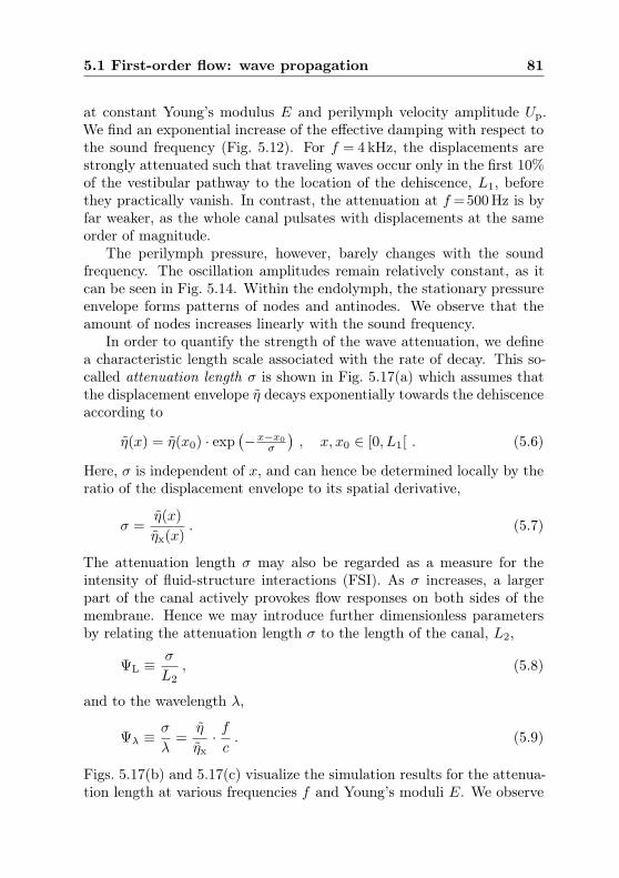
5.1 First-order flow: wave propagation 81

at constant Young’s modulus E and perilymph velocity amplitude Up.We find an exponential increase of the effective damping with respect tothe sound frequency (Fig. 5.12). For f = 4kHz, the displacements arestrongly attenuated such that traveling waves occur only in the first 10%of the vestibular pathway to the location of the dehiscence, L1, beforethey practically vanish. In contrast, the attenuation at f =500Hz is byfar weaker, as the whole canal pulsates with displacements at the sameorder of magnitude.

The perilymph pressure, however, barely changes with the soundfrequency. The oscillation amplitudes remain relatively constant, as itcan be seen in Fig. 5.14. Within the endolymph, the stationary pressureenvelope forms patterns of nodes and antinodes. We observe that theamount of nodes increases linearly with the sound frequency.

In order to quantify the strength of the wave attenuation, we definea characteristic length scale associated with the rate of decay. This so-called attenuation length σ is shown in Fig. 5.17(a) which assumes thatthe displacement envelope η decays exponentially towards the dehiscenceaccording to

η(x) = η(x0) · exp(−x−x0

σ

), x, x0 ∈ [0, L1[ . (5.6)

Here, σ is independent of x, and can hence be determined locally by theratio of the displacement envelope to its spatial derivative,

σ =η(x)

ηx(x). (5.7)

The attenuation length σ may also be regarded as a measure for theintensity of fluid-structure interactions (FSI). As σ increases, a largerpart of the canal actively provokes flow responses on both sides of themembrane. Hence we may introduce further dimensionless parametersby relating the attenuation length σ to the length of the canal, L2,

ΨL ≡ σ

L2, (5.8)

and to the wavelength λ,

Ψλ ≡ σ

λ=

η

ηx· fc. (5.9)

Figs. 5.17(b) and 5.17(c) visualize the simulation results for the attenua-tion length at various frequencies f and Young’s moduli E. We observe

82 Results and Discussion

x=0 L1 L2

−2

−1

0

1

2

Dis

pla

cem

entη[µm] envelope

η(t0)η(t0+1/8T )η(t0+2/8T )η(t0+3/8T )

(a) f = 500Hz

0 L1 L2

−2

−1

0

1

2

(b) f = 1kHz

0 L1 L2

−2

−1

0

1

2

(c) f = 2kHz

0 L1 L2

−2

−1

0

1

2

(d) f = 4kHz

Figure 5.12: Wave propagation along the membranous labyrinth for different soundfrequencies f at Young’s modulus E=40 kPa and perilymph velocity amplitude Up=2.6mm/s, visualized by consecutive snapshots of radial membrane displacements

(gray shades) and the corresponding envelope (red).

5.1 First-order flow: wave propagation 83

x=0 L1 L2

−50

−25

0

25

50

Vel

oci

tyηt[m

m/s]

envelopeηt(t0)ηt(t0+1/8T )ηt(t0+2/8T )ηt(t0+3/8T )

(a) f = 500Hz

0 L1 L2

−50

−25

0

25

50

(b) f = 1kHz

0 L1 L2

−50

−25

0

25

50

(c) f = 2kHz

0 L1 L2

−50

−25

0

25

50

(d) f = 4kHz

Figure 5.13: Wave propagation along the membranous labyrinth for different soundfrequencies f at Young’s modulus E = 40 kPa and perilymph velocity amplitudeUp=2.6mm/s, visualized by consecutive snapshots of radial membrane velocities

(gray shades) and the corresponding envelope (red).

84 Results and Discussion

x=0 L1 L2

−80

−40

0

40

80

Pre

ssure

pp[Pa]

envelopepp(t0)pp(t0+1/8T )pp(t0+2/8T )pp(t0+3/8T )

(a) f = 500Hz

0 L1 L2

−80

−40

0

40

80

(b) f = 1kHz

0 L1 L2

−80

−40

0

40

80

(c) f = 2kHz

0 L1 L2

−80

−40

0

40

80

(d) f = 4kHz

Figure 5.14: Wave propagation along the membranous labyrinth for different soundfrequencies f at Young’s modulus E = 40 kPa and perilymph velocity amplitudeUp = 2.6mm/s, visualized by consecutive snapshots of the perilymph pressure

(gray shades) and the corresponding envelope (red).

5.1 First-order flow: wave propagation 85

x=0 L1 L2

−80

−40

0

40

80

Pre

ssure

pe,Γ

[Pa]

envelopepe(t0)pe(t0+1/8T )pe(t0+2/8T )pe(t0+3/8T )

(a) f = 500Hz

0 L1 L2

−80

−40

0

40

80

(b) f = 1kHz

0 L1 L2

−80

−40

0

40

80

(c) f = 2kHz

0 L1 L2

−80

−40

0

40

80

(d) f = 4kHz

Figure 5.15: Wave propagation along the membranous labyrinth for different soundfrequencies f at Young’s modulus E = 40 kPa and perilymph velocity amplitudeUp = 2.6mm/s, visualized by consecutive snapshots of the endolymph pressure

(gray shades) and the corresponding envelope (red).

86 Results and Discussion

x=0 L1 L2

−r0

0

r0

Radia

lco

ord

inate

r 40

0

−40

40

0

−40

ux[m

m/s]

ur[m

m/s]

(a) f = 500Hz

0 L1 L2

−r0

0

r0

(b) f = 1kHz

0 L1 L2

−r0

0

r0

(c) f = 2kHz

0 L1 L2

−r0

0

r0

(d) f = 4kHz

Figure 5.16: Wave propagation within the endolymph for different sound frequenciesf at Young’s modulus E=40 kPa and perilymph velocity amplitude Up =2.6mm/s,visualized by snapshots of axial (r>0) and radial endolymph velocities (r<0).

5.2 Second-order flow: steady streaming in the endolymph 87

that the effective FSI length ΨL scales inversely with the frequency, asit was noted previously in Fig. 5.12. Stiffer membranes lead to higherwave speeds, and hence result in larger FSI lengths.

In all investigated combinations of f and E, the attenuation lengthΨλ varied between roughly one and two wavelengths, as can be seen inFig. 5.17(c). This may indicate that the wave attenuation is stronglycoupled to the stimulus frequency.

Keeping all other dimensionless parameters constant, the perilymphdominance β = Ap/Ae was varied between β = 5 and β = 20, coveringthe anatomical variance in human SCCs. The results of this study areshown in Fig. 5.18. One can see that the wave attenuation graduallyweakens as the perilymph increasingly dominates in size, suggesting thatthe endolymph generally contributes more strongly to the effective waveattenuation than the perilymph.

This aspect is further investigated in Fig. 5.19. The perilymph damp-ing was set to zero, i.e. ǫp = 0, and resulting membrane displacementsη are compared to the standard case where pseudo-viscous damping ap-plies, i.e. ǫp = ω. As there is no flow resistance in the perilymph forǫp = 0, the passive arm of the SCC exhibits unnaturally strong reflec-tions at the utricle boundary. These oscillations propagate upstreamand create interference patterns on the membrane envelope. However,regardless of the unphysical side effects, the overall decay of the waveamplitudes is only slightly affected by the change in perilymph damping.

5.2 Second-order flow: steady streaming in the en-

dolymph

The present section analyses the temporal average of the endolymphmotion at the periodic steady-state. First, we observe the local steadystreaming ue(x, r) from both the Eulerian and the Lagrangian perspec-tive, and comment on the resulting Stokes drift (Section 5.2.1). Thebulk streaming Ue(x) denotes the cross-sectional average of the localmean and represents the key parameter which connects the inner-eardynamics to the eye response of Tullio patients. With regard to Ue, asensitivity study is carried out in Section 5.2.2, making use of the dimen-sionless parameters which we obtained from the dimensional analysis inChapter 3.3. In Section 5.2.3 we assess different sources of nonlinearityand quantify their effect on the steady streaming in the endolymph.

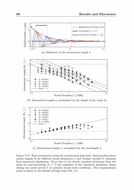
88 Results and Discussion

x=0 L1 L2

0

1

Dis

pla

cem

entη[µm]

displacement envelope η(x)

wavelength λ = c/f

attenuation length σ = η

ηx

(a) Definition of the attenuation length σ

0.1 1 10

0.1

1

Sound frequency f [kHz]

Att

enuation

length

ΨL[−

]

E=80 kPaE=40 kPaE=20 kPaE=10 kPaslope: −1

(b) Attenuation length σ, normalized by the length of the canal L2

0.1 1 100

1

2

3

4

Sound frequency f [kHz]

Att

enuation

length

Ψλ[−

]

E=80 kPaE=40 kPaE=20 kPaE=10 kPaE=5kPaE=2.5 kPaslope: 1

(c) Attenuation length σ, normalized by the wavelength λ

Figure 5.17: Wave attenuation along the membranous labyrinth: dimensionless atten-uation lengths Ψ for different sound frequencies f and Young’s moduli E, obtainedfrom numerical simulations. Error bars in (b) denote standard deviations from themean by post-processing Nt = T/∆t snapshots of the simulated membrane shapeduring one sound period T at periodic steady-state conditions. The computationalsetup is based on the default settings from Tab. 4.3.

5.2 Second-order flow: steady streaming in the endolymph 89

5 10 20

1

1.5

2

2.5

Perilymph dominance β=Ap/Ae

Att

enuation

length

Ψλ[−

]

E=80 kPa

E=40 kPa

E=20 kPa

E=10 kPa

Figure 5.18: Attenuation length Ψλ=σ/λ for different area ratios between perilymphand endolymph, β, and Young’s moduli E at sound frequency f=1kHz.

x=0 L1 L2

−1.5

−1

−0.5

0

0.5

1

1.5

Dis

pla

cem

entη[µm]

envelopeη(t0)η(t0+1/8T )η(t0+2/8T )η(t0+3/8T )

(a) ǫp = ω

0 L1 L2

−1.5

−1

−0.5

0

0.5

1

1.5

(b) ǫp = 0

Figure 5.19: Wave propagation along the membranous labyrinth (a) with and (b)without flow damping in the perilymph. Simulated at sound frequency f = 1kHz,Young’s modulus E=40 kPa and perilymph velocity amplitude Up=2.6mm/s. Visu-alized by consecutive snapshots of radial membrane displacements (gray shades) andthe corresponding envelope (red).

90 Results and Discussion

5.2.1 Eulerian and Lagrangian mean flow

Instantaneous values of the endolymph velocity are acquired for a dis-crete number of Nt time steps of length ∆t within one sound periodNt∆t = T = 1/f . In the following, we will apply different methods tocalculate the temporal mean of the flow field.

The Eulerian mean ue,E is defined at a fixed point in space (x, r) andcorresponds to the average over Nt successive values of the instantaneousendolymph velocity,

ue,E(x, r) ≡1

T

t0+T∫

t0

ue(x, r, t)dt ≈∆t

T

Nt∑

n=1

ue(x, r, tn) . (5.10)

As the numerical grid moves during simulation, we used the OpenFOAMlibrary to interpolate the flow field at each time step with the so-calledcellPointFace scheme applying mixed linear weights, documented inOpenFOAM Foundation (2015).

The Lagrangian mean ue,L refers to the mean distance a fluid particletravels during one sound period T ,

ue,L(x, r) ≡xP(t0 + T )− xP(t0)

T, xP(t0) =

[xr

]

, (5.11)

following a particle trajectory xP(t),

xP(t) ≡ xP(t0) +

t∫

t0

ue(xP(t), t)dt . (5.12)

We calculate the trajectory (5.12) with the explicit method of Heun. Attime t0, passive tracer particles are inserted into the endolymph anddistributed homogeneously across the whole domain. Advancing in time,we calculate a preliminary guess xP(t

n+1) of the new particle positionsby

xP(tn+1) = xP(t

n) + ue(xP(tn), tn)∆t . (5.13)

We interpolate the endolymph velocity at the estimated location xP andobtain the new particle position according to Heun’s method by

xP(tn+1) = xP(t

n) +ue(xP(t

n), tn) + ue(xP(tn+1), tn)

2∆t . (5.14)

5.2 Second-order flow: steady streaming in the endolymph 91

The Stokes drift ue,S is the difference between the Eulerian and theLagrangian mean,

ue,S(x, r) ≡ ue,E(x, r)− ue,L(x, r) . (5.15)

Fig. 5.20 shows results on the mean flow field of the endolymph. Weobserve that the Eulerian mean streams at largest amplitudes in thevicinity of the ampulla, featuring a positive flow adjacent to the walland a backflow at the centerline. In this entry region, propagating mem-brane displacements feature stronger amplitudes, as described in theprevious section. Similar to the attenuation of first-order waves alongthe canal, the steady endolymph streaming relaxes its cross-sectional pro-file towards a Poiseuille shape within the passive arm, cf. Fig. 5.20(d).The flow resistance to steady streaming may hence be approximated asa steady Poiseuille flow, in accordance with our model assumptions inChapter 3.2.4.

We note that the Eulerian and Lagrangian means coincide behindthe dehiscence, such that the Stokes drift on fluid particles becomes zeroin that area.

By principles of mass conservation, the overall volume flux stays con-stant along the canal. Hence a uni-directional, non-zero steady stream-ing is identified, revealing an effective transport of fluid in ampullofugaldirection, i.e. from the stapes towards the dehiscence.

5.2.2 Bulk flow analysis

The bulk streaming of the endolymph, Ue, is defined by the cross-sectional average over the local, axial mean flow ue|x ≡ ue, regardlessof the computational perspective (Eulerian or Lagrangian),

Ue(x) ≡1

r20π

∫

Ae

ue(x, r)dAe , (5.16)

and is constant along the canal due to conservation of mass, i.e.

∂

∂x

(Ue

)= 0 . (5.17)

Thus, for any tripel of the sound frequency f , Young’s modulus E andthe perilymph velocity amplitude Up we obtain from the numerical simu-lation one scalar value for the bulk endolymph streaming Ue. We may de-

92 Results and Discussion

x=0 L1 L2

0

r=r0

(a) Eulerian mean ue,E

0 L1 L2

0

r0

(b) Lagrangian mean ue,L

0 L1 L2

0

r0

ue[m

m/s]

−0.5

0

0.5

(c) Stokes drift ue,S = ue,E − ue,L

0.5 mms

L2L1x=0−r0

0

r=r0

ue,E

ue,L

ue,S

(d) Mean axial velocity profiles

Figure 5.20: Axial mean of the endolymph velocity, ue, viewed from an (a) Eulerianand (b) Lagrangian perspective, along with the resulting (c) Stokes drift. (d) Cross-sectional profiles of the axial mean velocities. Simulated for sound frequency f=1kHz,Young’s modulus E=40 kPa and perilymph velocity amplitude Up=2.6mm/s. Dataacquisition and post-processing by Benner (2015).

5.2 Second-order flow: steady streaming in the endolymph 93

fine a dimensionless variable for the bulk flow by introducing the stream-ing Reynolds number Re,

Re ≡ Ue2r0νf

. (5.18)

In the following, we intend to derive an analytical fit for Re, based ona sensitivity study with respect to variations of the Womersley numberWo (3.40), the Korteweg number Ko (3.37) and the Reynolds number Re

(3.39), since

Wo2 ∝ f , (5.19a)

Ko2 ∝ E , (5.19b)

Re ∝ Up . (5.19c)

We intend to confine the analytical fit to a physically reasonable parame-ter space which corresponds to realistic variances in the human inner earmorphology and material properties. Once the fit has been obtained, weare able to circumvent expensive numerical simulations. It can then bechained directly into our lumped parameter approach displayed in Fig.3.3.

We begin with the effects of the stapes velocity amplitude Up onthe formation of a steady endolymph flow. The results of Section 5.1revealed that the first-order flow scales linearly with Up. However, inFig. 5.21 we find that the second-order flow scales quadratically with Up,

Re ∝ Re2 . (5.20)

Furthermore, we detect a frequency shift of the bulk streaming patternwhen increasing Young’s modulus E of the membrane from E=40 kPato E=80 kPa. It appears that this shift correlates with the shift in thering frequency fπ (5.4) which marks the onset of a stop band for wavepropagation (Gautier et al., 2007). Hence we introduce a dimensionlessparameter for the ring frequency, Π, which can be expressed by a subsetof the other dimensionless parameters (3.37)-(3.44),

Π ≡ f

fπ=

Wo2

Ko

√

1− ν2sL . (5.21)

Taking into account the shape of the bulk streaming pattern from Fig.5.21(a), we approximate the strength of the steady streaming by

Re ∝ log10

(Π

K4

)

·(1−Π

1 + Π

)K5

, (5.22)

94 Results and Discussion

0.1 1 10

1

10

100

fπ

Sound frequency f [kHz]

Ue[µm/s]

Up=Up,0

Up=Up,0/2Up=Up,0/4Analytical fit (5.24)

(a) E = 40 kPa

0.1 1 10

1

10

100

fπ

Sound frequency f [kHz]

(b) E = 80 kPa

0.1 0.25 0.5 1

1

10

100

Perilymph velocity amplitude Up/Up,0 [−]

E=40 kPaE=80 kPaAnalytical fit (5.24), Ue ∝ U2

p

(c) f = 1kHz

Figure 5.21: Steady endolymph streaming Ue from numerical simulations for differentsound frequencies f and Young’s moduli E, setting the perilymph velocity amplitudeUp to a constant value. Up,0 =U⋆

s (f0, SPL0) = 2.6mm/s, with f0 = 1kHz, SPL0 =120 dB and U⋆

s from Fig. 1.11 (data labeled ‘Human cadaveric’). The ring frequencyfπ (5.4) is indicated by a dotted vertical line, marking the onset of a stop band foracoustic wave propagation according to Gautier et al. (2007). Dashed lines in (a) and(b) correspond to horizontal cuts of the contour plot in Fig. 5.23(a). Data acquisitionby Benner (2015).

5.2 Second-order flow: steady streaming in the endolymph 95

where Π = K4 corresponds to the low-frequency limit at zero bulk ve-locity, and the ring frequency at Π = 1 marks the upper limit at waveevanescence. The constant K5 defines the sharpness of the upper limit.

In order to test the robustness of the derived proportionalities in(5.20) and (5.22), we apply the frequency-dependent, anatomical spreadof stapes velocities Us at the perilymph boundary. Setting the peri-lymph velocity amplitude Up equal to the stapes velocity measurementsby Kringlebotn & Gundersen (1985) at SPL=120 dB (Fig. 1.11), we re-run our numerical simulation series for different f and E. The resultsare displayed in Fig. 5.22.

Since the anatomical reference features a maximum of the stapesmotility at f ≈1 kHz, the steady streaming becomes strongest in a sim-ilar range. This observation is well in accordance with the quadraticdependence (5.20) of the bulk streaming Ue on the stapes velocity am-plitude Up.

As we divide the simulated bulk velocities by (5.20) and (5.22), weidentify a further dependency related to the excitability of the membrane,which we approximate by

Re ∝ ΠK2

Wolog10

(K3Wo

Π

)

. (5.23)

The membrane excitability (5.23) will be revisited in Fig. 5.29(b) ofSection 5.4. The dimensionless fit for the Reynolds number of the steadyendolymph streaming Re thus becomes

Re = K1Re2ΠK2

Wolog10

(K3Wo

Π

)

log10

(Π

K4

)(1−Π

1 + Π

)K5

, (5.24)

valid for Π ∈ [K4, 1], with constants Ki from Tab. 5.1. In the stop bandfor wave propagation, we assume that the bulk streaming vanishes, i.e.

Re!= 0 , Π > 1 . (5.25)

Fig. 5.23(a) shows a contour plot of the analytical fit in dimensionalquantities for a constant perilymph velocity amplitude Up. Although aconstant Up does not reflect the reality, the graph enables us to visuallyisolate the streaming mechanisms from their dependence on the anatom-ical boundary conditions. We find that the steady streaming is generallystrongest for frequencies f△ at

Π△=f△/fπ≈1

3, (5.26)

96 Results and Discussion

1 10 1000

0.1

0.2

Young’s modulus E [kPa]

Ste

ady

stre

am

ingUe[m

m/s]

f=1kHz, Up=2.6mm/s

f=640Hz, Up=2.1mm/s

f=2kHz, Up=1.2mm/s

f=320Hz, Up=0.94mm/s

Analytical fit (5.24)

(a)

0.1 1 100

0.05

0.1

Sound frequency f [kHz]

Ste

ady

stre

am

ingUe[m

m/s]

E=20 kPa

E=40 kPa

E=80 kPaAnalytical fit (5.24)

(b)

Figure 5.22: Steady endolymph streaming Ue for different sound frequencies f andYoung’s moduli E, assuming that perilymph velocity amplitudes Up are a function ofthe stapes motility U⋆

s (f, SPL0). U⋆s from Fig. 1.11 (data labeled ‘Human cadaveric’),

with SPL0 =120 dB. Symbols denote simulation results, dashed lines correspond to(a) vertical and (b) horizontal cuts of the contour plot in Fig. 5.23(b).

K1 K2 K3 K4 K5

1.26 0.3 6.76 0.018 0.1

Table 5.1: Fitting constants in (5.24) for the steady streaming Reynolds numberRe(Re,Wo,Π) at perilymph dominance β = 10, fluid loading L = 13.3, membraneweight γ = 1.2, location of the dehiscence κ1 = 31.25 and canal length κ2 = 56.25.Dimensionless parameters are defined in (3.37)-(3.44), (5.18), (5.21).

5.2 Second-order flow: steady streaming in the endolymph 97

and that it increases monotonically along isolines of Π towards softermembranes and lower frequencies. It may be remarked that Π scalesinversely with the wavelength λ,

λ ≈ cKf

∝√E

f∝ fπ

f=

1

Π, Π ≪ 1 . (5.27)

Therefore isolines of Π also correspond to isolines of λ. At Π△, thewavelength λ△ fits approximately six times into the length of the activearm, L1.

Fig. 5.23(b) already captures the anatomical frequency dependence ofthe stapes motility Us(f) according to data by Kringlebotn & Gundersen(1985) from Fig. 1.11. We note that the anatomical constraints restrictthe streaming corridor from the previous figure to a spot around f =1kHz.

The most realistic scenario is displayed in Fig. 5.23(c). It accountsfor both the anatomy and the SCD pathology, since it incorporates thelumped lever arm model (3.1) described in Chapter 3.1. According tothe model, part of the stapes-induced perilymph motion diverts into thecochlear scalae, alleviating the bulk streaming from Fig. 5.23(b) at higherfrequencies (cf. Fig. 1.12). Additionally, the lever arm between the stapesfootplate and the smaller SCC lumen increases the perilymph velocityamplitudes Up linearly, and hence the bulk streaming Ue quadratically.

The influence of the dehiscence location L1 on the steady endolymphstreaming Ue was assessed by numerical simulations. Results are shownin Fig. 5.24(a). We find that a shift of the dehiscence further away fromthe ampulla results in an increase of streaming amplitudes. This maycorrelate with an increase in the active membrane surface. However,it may be remarked that longer perilymph pathways L1 increase theflow resistance in the vestibular system, possibly lowering the velocityamplitudes Up which are diverted towards the dehiscence. Such an effectwas not accounted for, and may result in a less pronounced increase inFig. 5.24(a).

Fig. 5.24(b) shows a similar study varying the total length of the slen-der duct, L2. As the flow resistance scales with L2, the steady streamingbehaves inversely proportional to the canal length.

5.2.3 Sources of nonlinearity

A system which features only linear mechanisms is unable to exhibitsecond-order phenomena. Although the involved fluids of the vestibularsystem behave practically linearly in everyday head maneuvers, the spe-

98 Results and Discussion

0.1 1 10

1.25

2.5

5

10

20

40

80

160

➁

➀

Young’s

modulu

sE

[kPa]

(a) Up = U⋆s (f0, SPL0)

0.1 1 10

1.25

2.5

5

10

20

40

80

160

(b) Up = U⋆s (f, SPL0)

0.1 1 10

1.25

2.5

5

10

20

40

80

160

Sound frequency f [kHz]

Ue[m

m/s]

0

0.04

0.08

0.12

0.16

(c) Up = U⋆p (φ⋆(f), U⋆

s (f, SPL0))

Figure 5.23: Contour plots of steady endolymph streaming Ue as function of soundfrequency f , Young’s modulus E and perilymph velocity amplitude Up. Circles indi-cate results from numerical simulations, from which the analytical fit (5.24) has beenderived. Ue reverses its direction in region ➀. The dashed line (red) corresponds tothe ring frequency fπ (5.4), marking the onset of stop band region ➁ for acousticplane waves, according to Gautier et al. (2007). Thick isolines correspond to valuesprinted in the color bar. f0=1kHz, SPL0=120 dB, U⋆

p from (3.1), U⋆s from Fig. 1.11,

φ⋆ from Fig. 1.12. Further physical and numerical parameters are given in Tab. 4.3.

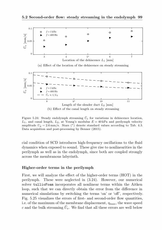
5.2 Second-order flow: steady streaming in the endolymph 99

3 4 5⋆ 6 70

0.05

0.1

Location of the dehiscence L1 [mm]

Ue[m

m/s]

f=1kHz

f=400Hz

(a) Effect of the location of the dehiscence on steady streaming

8 9⋆ 10 110

0.05

0.1

Length of the slender duct L2 [mm]

Ue[m

m/s]

f=1kHz

f=400Hz

Ue ∝ 1/L2

(b) Effect of the canal length on steady streaming

Figure 5.24: Steady endolymph streaming Ue for variations in dehiscence location,L1, and canal length, L2, at Young’s modulus E = 40 kPa and perilymph velocityamplitude Up = 2.6mm/s. Stars (⋆) denote standard values according to Tab. 4.3.Data acquisition and post-processing by Benner (2015).

cial condition of SCD introduces high-frequency oscillations to the fluiddynamics when exposed to sound. These give rise to nonlinearities in theperilymph as well as in the endolymph, since both are coupled stronglyacross the membranous labyrinth.

Higher-order terms in the perilymph

First, we will analyze the effect of the higher-order terms (HOT) in theperilymph. These were neglected in (3.24). However, our numericalsolver tullioFoam incorporates all nonlinear terms within the Aitkenloop, such that we can directly obtain the error from the difference innumerical simulations by switching the terms ‘on’ or ‘off’, respectively.Fig. 5.25 visualizes the errors of first- and second-order flow quantities,i.e. of the maximum of the membrane displacement, ηmax, the wave speedc and the bulk streaming Ue. We find that all these errors are well below

100 Results and Discussion

unity. Most importantly, the second-order flow in the endolymph isaffected by less than three orders of magnitude. Hence we conclude thathigher-order terms can safely be neglected, as they do not contributesignificantly to the Tullio phenomenon.

10 10010−6

10−5

10−4

10−3

10−2

10−1

Young’s modulus E [kPa]

Rel

ative

erro

rsε η

,ε u

,ε c

[−]

displacement ηmax

steady streaming Ue

wave speed c

Figure 5.25: Relative errors ε due to neglects of higher order terms (HOT) in theperilymph, corresponding to numerical simulations (w/ and w/o HOT) at soundfrequency f=1kHz. Displayed are errors of first-order (max. membrane displacementηmax, wave speed c) and second-order flow quantities (steady endolymph streamingUe). Absolute errors are normalized by the magnitude of the respective flow quantity.

Nonlinearities in the endolymph

Within the endolymph, further mechanisms are able to create second-order flow components. First of all, as the Navier-Stokes equationscomprise the nonlinear advection term, Reynolds stresses may drive themean flow. We carried out numerical simulations to assess the influenceof these stresses on the bulk streaming, comparing cases when advectionwas switched ‘on’ or ‘off’.

Fig. 5.26 visualizes the results for different Young’s moduli E andsound frequencies f . Although all nonlinear terms in the governingequations are suppressed, we still obtain a non-zero mean flow. Ob-viously there is a second streaming mechanism at play which can onlycorrespond to nonlinearities in the FSI coupling at the interface. A sim-ilar phenomenon has been observed for steady streaming in the cochlea(Edom et al., 2014). We denote this type of flow by ‘wall-induced’streaming Ue|w. The difference in streaming, Ue|Re, thus relates to theReynolds forcing,

Ue

∣∣Re

≡ Ue − Ue

∣∣w. (5.28)

5.3 Eye response to sound stimuli 101

10 20 40 80

−0.1

0

0.1

0.2

Young’s modulus E [kPa]

Ue[m

m/s]

(a) f = 1kHz

0.64 0.8 1 1.25 1.6

−0.1

0

0.1

0.2

Sound frequency f [kHz]

Ue

Ue

∣

∣

Re≡ Ue − Ue

∣

∣

w

Ue

∣

∣

w

(b) E = 40 kPa

Figure 5.26: Steady endolymph streaming Ue from numerical simulations, with andwithout nonlinear contributions from the advection term in the Navier-Stokes equa-tions (Reynolds stresses). Results are visualized for different sound frequencies f andYoung’s moduli E at constant perilymph velocity amplitude, Up,0 =2.6mm/s. Thesteady streaming which originates from Reynolds stresses is denoted by Ue

∣

∣

Re, and

is obtained from the difference in Ue when advection was suppressed, i.e. when onlysteady streaming Ue

∣

∣

wfrom nonlinearities of the wall motion is present.

Fig. 5.26 shows that the Reynolds streaming contribution stays constantfor changes in the membrane stiffness, but varies significantly with thefrequency. Low stimulus frequencies apparently weaken the degree ofnonlinearity from the Reynolds stresses. The Reynolds streaming rep-resents the major part of the steady endolymph flow and is stronger inmagnitude than the wall-induced contributions.

It is interesting to see that the wall-induced streaming reverses itsdirection above a certain membrane stiffness, indicating that there existsat least one stimulus frequency f for a given stiffness E at which Ue|wvanishes completely.

5.3 Eye response to sound stimuli

A patient presenting with the Tullio phenomenon may sense dizzinessand experience vertigo when exposed to loud sound stimuli. As theseare rather subjective symptoms which can hardly be quantified, one looksfor secondary effects such as the eye response to vestibular stimulation.The cupula mechanics in combination with the vestibulo-ocular reflex

102 Results and Discussion

(VOR) translates the induced endolymph flow into a motion of the eye,with a slow-phase velocity component αt. In Chapter 3.2.4 we demon-strated that these velocities scale directly proportionally to the steadyendolymph streaming Ue by

αt ≈ KsUe , (5.29)

with a proportionality constant Ks ≈ 191◦/mm. In the course of a sen-sitivity study, we obtained an analytic expression (5.24) for the steadyendolymph streaming Ue from numerical simulations, i.e.

Ue =νf2r0

Re(

Re ∝ Up,Wo ∝√

f ,Ko ∝√E)

. (5.30)

The perilymph velocity amplitude Up relates to the (patho-)anatomy ofthe specific Tullio patient. This may be estimated by our lumped leverarm model (3.1), being a function of the cochlear admittance φ, theanatomical ratio of the stapes footplate area As to the perilymph lumenAp, the stapes motility Us/ps and the sound pressure level SPL,

Up(f, SPL, D) =As

Ap· (1− φ(f,D)) · Us

ps(f) · pref10

SPL20 dB , (5.31)

where D denotes the radius of the dehiscence rd relative to the canalradius rSC, as in Kim et al. (2013). Once the patho-anatomical referencedata are obtained, e.g. by

φ = φ(f,D) from Kim et al. (2013) , (5.32)

Us

ps=

Us

ps(f) from Kringlebotn & Gundersen (1985) , (5.33)

the slow-phase eye velocities αt can be directly calculated for any har-monic sound stimulus using (5.29)-(5.31).Fig. 5.27 shows our model predictions on the slow-phase eye velocitiesαt for a sound pressure level of SPL = 110 dB, and compares them toreference data from different Tullio patients in the literature.

In order to account for anatomical variations among subjects, we ad-ditionally shifted the stapes characteristics Us(f) of the anatomical ref-erence (➁,➄) by Kringlebotn & Gundersen (1985) to lower (➀,➃) andhigher (➂) frequencies. The effect of the size of the dehiscence D wasassessed by using predictions on the cochlear admittance φ(f,D) from

5.3 Eye response to sound stimuli 103

0.1 1 10

0.01

0.1

1 ➀ ➁ ➂

➃ ➄

Sound frequency f [kHz]

Up,Us[m

m/s]

,φ[−

]←

Size

ofdeh

iscence

D→

← Anatomical variance in stapes motility Us (frequency shift) →

Us=U⋆s (2f)

φ=φ⋆(f,D1)

Us=U⋆s (f)

φ=φ⋆(f,D1)

Us=U⋆s (0.5f)

φ=φ⋆(f,D1)

Us=U⋆s (2f)

φ=φ⋆(f,D0.1)

Us=U⋆s (f)

φ=φ⋆(f,D0.1)

Perilymph vel. amp. Up

Stapes vel. amp. Us

Cochlear admittance φ

(a) Possible scenarios of (patho-)anatomical conditions in patients with SCD

0.1 1 10

0.1

1

10➀ ➁ ➂

➃ ➄

Sound frequency f [kHz]

Eye

vel

oci

tyαt[◦/s]

←Size

ofdeh

iscence

D→

E=20 kPa

E=40 kPa

E=80 kPaKaski(2012), Fig.8

Minor(2005), Fig.1

Minor(2001), Fig.1

Minor(2001), Fig.6

Minor(2000), Fig.1

Cremer(2000b), Fig.1

Cremer(2000b), Fig.4

Cremer(2000b), Fig.5

(b) Corresponding predictions of the slow-phase eye velocities αt

Figure 5.27: Comparison of predicted slow-phase eye velocities αt from five virtualpatients (➀-➄) with measurement data from nine real patients at a sound pressurelevel of SPL = 110 dB. Physioanatomical conditions correspond to stapes motilitymeasurements U⋆

s by Kringlebotn & Gundersen (1985), displayed in Fig. 1.11, la-beled ‘Human cadaveric’. SCD pathoanatomy relates to numerical predictions of thecochlear admittance φ⋆ by Kim et al. (2013), displayed in Fig. 1.12 for different sizesof the dehiscence, D≡rd/rSC, where D1 = 1, D0.1 = 0.1. Perilymph velocity ampli-tudes Up obtained from (3.1) with stapes footplate area As=3.21mm2 (Aibara et al.,2001) and perilymph lumen Ap=βr20π. Further parameters are listed in Tab. 4.3.

104 Results and Discussion

Kim et al. (2013) for D=1 (➀,➁,➂) and D=0.1 (➃,➄). The correspond-ing graphs are shown in Fig. 5.27(a).

The eye velocity predictions from our fluid-dynamical model corre-spond well with the typical range of patient responses from the literature,e.g. by Cremer et al. (2000b), Minor (2000), Minor et al. (2001), Minor(2005) and Kaski et al. (2012). Within the tested anatomical varianceamong the virtual patients ➀-➄, the symptoms of already five out ofeight real patients can be explained by our model.

Generally we note that the peak sensitivity for the Tullio phenomenoncoincides with the peaks in stapes motility Us(f). An anatomical vari-ance in the membrane stiffness E plays a role predominantly at soundfrequencies around these sensitivity peaks and below, with stiffer mem-branes increasingly alleviating pathological symptoms.

We further observe that smaller dehiscence radii rd shift the peakresponse slightly towards lower frequencies and reduce the intensity ofthe Tullio phenomenon by roughly

∂ log10(αt/[◦/s])

∂ log10(rd/rSC)≈ 0.64 , rd ≤ rSC . (5.34)

The effect of the dehiscence location L1 was shown in Fig. 5.24(a) forfrequencies of f = 0.4 kHz and f = 1kHz. Although we remarked thatthe true increase of Ue (∝ αt) with L1 is probably slightly weaker thandisplayed, the effect of L1 on the Tullio phenomenon is on a similar orderas the effects from the dehiscence size, i.e.

∂ log10(αt/[◦/s])

∂ log10(L1/r0). 0.66 , L1 ≫ r0 . (5.35)

The values for the slopes in (5.34)-(5.35) correspond to respective aver-ages over the available data, and vary slightly with E and f .

Fig. 5.28 shows additionally the effect of the sound pressure levelon the Tullio phenomenon. If we assume that the subjective feeling ofvertigo and dizziness grows equally in strength as the corresponding eyemotions, we may suppose that there exists a measurable threshold αt,min

below which a Tullio patient does not experience vestibular responses tosound. With regard to physiological operating ranges of the vestibularsystem, rotational head motions with velocities on the order of 0.1◦/sare located at the low-frequency end of the balance sense. Thus we mayregard the corresponding isocontour of the eye response as a conceivable

5.3 Eye response to sound stimuli 105

0.1 1 10

100

110

120

fπ

SPL

[dB]

αt[◦/s]

0.1

1

10

(a) E = 20 kPa

0.1 1 10

100

110

120

fπ

(b) E = 40 kPa

0.1 1 10

100

110

120

fπ

Sound frequency f [kHz]

(c) E = 80 kPa

Figure 5.28: Activity map of the Tullio phenomenon for the virtual patient ➁ of theprevious figure. Contour plots of the predicted slow-phase eye velocity αt correspondto our model (5.29)-(5.33), and are shown as a function of the sound frequency fand the sound pressure level SPL. The dashed line (red) corresponds to the ringfrequency fπ (5.4), marking the onset of a stop band region for acoustic plane wavesaccording to Gautier et al. (2007). Physical parameters are given in Tab. 4.3.

106 Results and Discussion

threshold for the Tullio phenomenon, i.e. at

αt,min≈0.1◦/s . (5.36)

Showing only isocontours of αt ≥ 0.1 ◦/s, Fig. 5.28 basically reveals theactivity map of the Tullio phenomenon. In the white space, the associ-ated vestibular responses are too weak to produce perceivable symptoms.In the active region, a ‘sweet spot’ for vestibular reactions can be deter-mined for each sound pressure level. We qualitatively observe that thisspot narrows for stiffer membranous labyrinths. This coincides with thefrequency shift of fπ which moves the peak of steady streaming sensi-tivity (Π△≈ 1/3 (5.26), Fig. 5.23(a)) away from the peak of the stapessensitivity towards higher frequencies.

Tullio patients may as well feature patho-anatomical conditionsslightly different from the ones which were suggested by Kim et al.(2013). If the cochlear admittance φ was less pronounced at higher fre-quencies, the perilymph would oscillate by stronger amplitudes Up. Asthe steady streaming scales quadratically with Up, this could explainthe three case reports from Fig. 5.27(b) which exhibited symptoms atf=2− 3 kHz.

However, it may also be possible that a further mechanism exists atvalues of approximately 0.5≤Π< 1 where our linear membrane modelis not able to resolve the increasing influence from longitudinal motionson the plane-wave propagation.

5.4 Discussion of the results

The results of our numerical simulations enabled us to establish an an-alytical formulation (5.24) for the Tullio phenomenon in the parameterrange of interest,

f ∈ [100Hz, 10 kHz] → Wo ∈ [4, 40] , (5.37a)

E ∈ [1 kPa, 100 kPa] → Ko ∈ [40, 400] , (5.37b)

Up ∈ [0mm/s, 10mm/s] → Re ∈ [0, 1.6] . (5.37c)

As we identified several mechanisms affecting the vestibular response tosound, we will highlight each of them separately in the following.

Nonlinear mechanisms

The governing equations of our computational model comprise two non-linear mechanisms: Reynolds stresses arising from the advection term

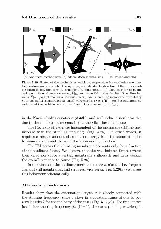
5.4 Discussion of the results 107

F |Re F |w ΨL ηmax φ Us/ps

(a) Nonlinear mechanisms (b) Attenuation mechanisms (c) Patho-anatomy

logE

logf

Π=K4

Π△

Π=1

Figure 5.29: Sketch of the mechanisms which are responsible for vestibular reactionsto pure-tone sound stimuli. The signs (+/−) indicate the direction of the correspond-ing mean endolymph flow (ampullofugal/ampullopetal). (a) Nonlinear forces in theendolymph from Reynolds stresses, F |Re, and from FSI in the vicinity of the vibratingwalls, F |w. (b) Optimal wave attenuation ΨL, and increasing membrane excitabilityηmax for softer membranes at equal wavelengths (λ ∝ 1/Π). (c) Pathoanatomicalvariance of the cochlear admittance φ and the stapes motility Us/ps.

in the Navier-Stokes equations (3.33b), and wall-induced nonlinearitiesdue to the fluid-structure coupling at the vibrating membrane.

The Reynolds stresses are independent of the membrane stiffness andincrease with the stimulus frequency (Fig. 5.26). In other words, itrequires a certain amount of oscillation energy from the sound stimulusto generate sufficient drive on the mean endolymph flow.

The FSI across the vibrating membrane accounts only for a fractionof the nonlinear forces. We observe that the wall-induced forces reversetheir direction above a certain membrane stiffness E and thus weakenthe overall response to sound (Fig. 5.26).

In combination, the nonlinear mechanisms are weakest at low frequen-cies and stiff membranes, and strongest vice versa. Fig. 5.29(a) visualizesthis behaviour schematically.

Attenuation mechanisms

Results show that the attenuation length σ is closely connected withthe stimulus frequency, since σ stays in a constant range of one to twowavelengths λ for the majority of the cases (Fig. 5.17(c)). For frequenciesjust below the ring frequency fπ (Π=1), the corresponding wavelength

108 Results and Discussion

λ is very small, such that the effective attenuation length ΨL = σ/L2

becomes very small as well. Therefore the membrane is hardly able toprovoke nonlinear reactions since the propagating waves ‘die out’ tooquickly.

We know from Gautier et al. (2007) that the wave propagation isevanescent (‘stop band’) in regions of Π≥1. Moving away from this stopband across isolines of Π in Fig. 5.29(b), the wave length λ increases.This yields a stronger vestibular response as the effective FSI area onthe membrane surface increases with λ.

However, above a certain wavelength λ△ ≈L1/6 the gain in steadystreaming is alleviated by the growing intensity of wave reflections, asthe weakly attenuated displacements reach the end of the canal. Whenwe approach the line of Π=K4, the wavelengths have reached the sizeof λ≈L2 and the steady streaming vanishes almost completely.

Along the ‘streaming corridor’ of optimal sensitivity, i.e. at Π△, an-other mechanism is able to enhance vestibular responses. Walking to-wards lower frequencies f and softer membranes E at constant wave-length λ, the membranous labyrinth becomes less resistive to transmuralloads. This results in larger displacement maxima ηmax which intensifythe pulsatile character of the endolymph response, and ultimately thesteady streaming.

Influence of the (patho-)anatomy

The superior canal dehiscence leads to a redistribution of the stapes-induced perilymph motion, away from the cochlear scalae. From predic-tions by Kim et al. (2013) we know how the cochlear admittance φ dropsin function of the sound frequency and the dehiscence size. At the low-frequency limit of hearing, practically all flow enters the vestibular sys-tem. The opposite happens at frequencies higher than f >500Hz, wherethe vestibular pathway features a larger impedance than the cochlea.Our computational model predicts that the Tullio phenomenon decreaseswith the square of the cochlear admittance, i.e.

αt ∝ Ue ∝ U2p ∝ (1− φ)2 . (5.38)

The stapes motility Us/ps exhibits an equally strong influence whichpeaks at approximately f = 1kHz according to measurements byKringlebotn & Gundersen (1985), Huber et al. (2001) and Chien et al.(2009). Since Us/ps decays in the log-log scale by a slope of 1 towards

5.4 Discussion of the results 109

both lower and higher frequencies, the resulting decay in eye motionamounts to a slope of 2. This imposes a sharp peak on the Tullio activ-ity map in Fig. 5.28, creating a ‘sweet spot’ for the phenomenon. Fig.5.29(c) visualizes the corresponding mechanisms.

Limitations of the computational model

Outside the range of Π ∈ [0.05, 0.5], the computational model approachesits limits both numerically and phenomenologically. As already men-tioned, at frequencies close to Π . 1 occur interdependencies with longi-tudinal waves within the membrane. These cannot be captured, as ourmodel accounts only for radial membrane oscillations. This could ex-plain why our predictions do not match the patient data at f=2−3 kHzin Fig. 5.27(b).

Additionally, a numerical restriction appears when the wavelengthλ becomes very small, i.e. λ ≪ r0. In this case, the necessary spatialresolution along the centerline coordinate x increases so heavily that itrenders a timely solution virtually impossible. Likewise, for very largewavelengths λ & L2, the FSI coupling algorithm fails to converge.

It may also be remarked that our computational model neglects fluidmotions along alternative pathways to the dehiscence. We believe thatthese do not contribute significantly to the observed phenomenon andsuch a scenario is not captured by our numerical simulations.

Chapter 6

Concluding Remarks and Outlook

Vestibular responses to sound in presence of a superior canal dehis-cence (SCD) obey intricate mechanisms of fluid-structure interaction. Inthe course of the present work, we sought to identify the key parameterswhich generate, enhance or weaken such misperceptions of the balancesense.

Based on a computational modeling approach from a primarilyfluid-dynamical perspective, we carried out numerical simulations ofpure-tone stimulations across the whole bandwidth of the audiblefrequency spectrum. For that purpose, we specifically designed atailor-made code which incorporates state-of-the-art methods to resolveinterdependencies between the inner-ear fluids and the membranouslabyrinth. The numerical solver was validated against similar studies onwave propagation in elastic tubes (Gautier et al., 2007), assuring thatour results are sound and in good agreement with the literature.

An analysis of the primary flow response revealed that the stapesvibrations induce traveling waves along the membranous labyrinth asthe perilymph begins to oscillate forth and back in the SCC. Exposedto oscillating transmural pressures, the elastic walls of the membranouslabyrinth displace and provoke further mechanical responses in the adja-cent fluids (endolymph and perilymph). On their pathway through thesemicircular canals towards the dehiscence, the waves are attenuated byviscous and inertial effects from both fluids. This attenuation was foundto be closely coupled to the frequency of the sound stimulus.

Within the vibrating membranous duct, the endolymph responds bystrong pulsations at sound frequency, thus continuously displacing thecupula forth and back. This behaviour might explain the observationsfrom animal experiments by Carey et al. (2004) who reported a phase-locking of irregular cupula afferents to the sound stimulus.

When we calculated the temporal mean of the primary endolymphoscillations, we identified a secondary, steady flow component. This

112 Concluding Remarks and Outlook

so-called steady streaming corresponds to a continuous pumping of fluiduni-directionally through the slender membranous canal until the cupulareaches a balanced offset displacement. We suspect that this mech-anism corresponds to the tonic behavior of regular cupula afferents(Carey et al., 2004).

Revisiting previous studies on the fluid dynamics of the balancesense during head rotation (Grieser et al., 2014c), we were able to linkthe cupula displacement to the resulting eye velocities. Furthermore, ananalytical formulation for the steady streaming was deduced from thesimulation results by means of a dimensional analysis.

Our predictions for the eye motion compare well with clinical datafrom patients with a superior canal dehiscence. It appears that the Tulliophenomenon is restricted to a ‘sweet spot’ in the sound spectrum. Thisspot is expected to shift due to the individual anatomy of the patient, asthe stapes oscillates strongest at certain sound frequencies (Chien et al.,2009). Additionally, this spot is confined by the degree of nonlinearityin the system response. Higher frequencies, if not overdamped, generallyyield stronger vestibular reactions.

However, when the sound frequency falls into the ‘stop band’ forwave propagation (Gautier et al., 2007) at roughly 4−6 kHz, the acousticwaves become evanescent and thus the phenomenon disappears. More-over, the impedance of the vestibular system outweighs the impedanceof the cochlear pathway at high frequencies (Kim et al., 2013), such thatthe balance sense becomes less responsive to sound.

We further noted that both the location and the size of the dehis-cence play a role in the Tullio phenomenon, although this is subordinateto the other effects: larger dehiscences further away from the stapesyield stronger responses.

The present thesis has identified mechanisms which may explain theTullio phenomenon. In order to confirm the validity of our predictions,follow-up studies may be carried out in vitro on upscaled models of themembranous labyrinth. Since we are providing an analytical correlationin dimensionless form, the corresponding experimental setup can be de-signed relatively easily by maintaining the dimensionless numbers.

Making minor modifications, our computational model could also beused to investigate more complex sound stimuli. If the reported sweetspot resonance can be canceled out by means of destructive interference

113

with other frequencies, one could actively suppress vestibular responses(‘intelligent earphones’). In such a scenario, the patient would haveto trade sensations of vertigo with the exposure to interference noise.Alternatively, using the modern technology of hearing aids, it isconceivable that the intensity of the incoming sound spectrum wereto be selectively attenuated. That way, vestibular reactions could bealleviated by lowering the sound pressure level of trigger frequencies forthe Tullio phenomenon.

We may conclude this thesis by emphasizing and confirming the state-ment by Rabbitt et al. (1999): ‘increasing the membrane stiffness wouldmake canal plugging more effective in attenuating cupular responses,whereas reducing the stiffness would cause the opposite’. If ways can befound to artificially stiffen the membranous labyrinth on the vestibularside, it should be possible to alleviate the symptoms for patients withSCD, maybe even without the need for surgery.

Appendix A

Pseudo-viscous damping

In the following we derive the pseudo-viscous parameter ǫp whichmodels the damping characteristics of the perilymph in strongly pulsat-ing flows such as they occur in the Tullio phenomenon. ǫp was intro-duced in the momentum equation (3.17) and attempts to capture radialcontributions from viscous stresses and inertial effects which cannot beresolved by the one-dimensional model given by

1

Ap

∂ (Apup)

∂t+ ǫpup = − 1

ρf

∂pp∂x

. (A.1)

Obrist (2014) obtained an exact solution for unsteady pipe flows withharmonic forcing,

u(r, t) =i

ω·(

1− J0(i3/2Wo r/a)

J0(i3/2Wo)

)

· 1

ρf

∂p

∂x(t) , (A.2)

where J0 denotes the Bessel function of first kind and zeroth order, i theimaginary unit, a the pipe radius and Wo the Womersley number,

Wo ≡ a

δν= a

√ω

νf, (A.3)

related to the Stokes boundary layer thickness δν . Integration of (A.2)in the radial direction r′≡r/a leads to the bulk velocity U ,

U(t) =a2∫ 1

0[u(r′, t) · 2πr′] dr′

a2π=

Wω

· 1

ρf

∂p

∂x(t) , (A.4)

where W is a dimensionless and complex-valued function of the Womers-ley number,

W = 2i

∫ 1

0

(

1− J0(i3/2Wo r′)

J0(i3/2Wo)

)

r′dr′ . (A.5)

A steady (Wo≪1), laminar (Re≪1) pipe flow results from the balanceof viscous stresses with the pressure gradient, i.e.

−νf

(1

r

∂

∂r

(

r∂

∂ru(r)

))

= − 1

ρf

∂p

∂x. (A.6)

116 Pseudo-viscous damping

The solution of (A.6) can be directly obtained from the Hagen-Poiseuille

law, stating that the bulk velocity UHP is identical to

UHP = − a2

8νf· 1

ρf

∂p

∂x. (A.7)

In other words, the viscous stresses on the left-hand-side of (A.6) scalelinearly with the bulk velocity UHP as

−νf

(1

r

∂

∂r

(

r∂

∂ru(r)

))

= ǫHPUHP , (A.8)

with a proportionality constant ǫHP given by

ǫHP =8νfa2

=8ω

Wo2. (A.9)

Since the right-hand side of (A.8) resembles our pseudo-viscous modelterm in the momentum balance (A.1), we may postulate that

ǫHP UHP = ǫHPUHP

U(t)U(t)

!= ǫHP

∣∣∣∣

UHP

U(t)

∣∣∣∣

︸ ︷︷ ︸

≡ǫp

up = ǫpup , (A.10)

such that the pseudo-viscous damping becomes

ǫp = ω1

|W| = ǫHPWo2/8

|W| . (A.11)

10−1 100 101 102 10310−4

10−2

100

102

104

106

Womersley number Wo

|W|

|W|

Wo2/8

Figure A.1: Correction factor |W| for the pseudo-viscous damping ǫp, obtained fromnumerical evaluations of the complex-valued integral in (A.5) in function of the Wom-ersley number Wo (A.3) with a radial resolution of 1000 computational nodes.

117

Fig. A.1 shows how the pseudo-viscous damping ǫp recovers the Hagen-Poiseuille limit ǫHP at flows of low Womersley numbers where W becomesWo2/8 and thus

ǫp ≈ ǫHP , Wo ≪ 1 . (A.12)

Towards the upper limit at high Womersley numbers, the damping ǫpbecomes identical to the angular frequency ω of the sound stimulus,

ǫp ≈ ω , Wo ≫ 1 . (A.13)

Since the stapes-induced flows within the perilymph are characterizedby high Womersley numbers significantly larger than unity, expression(A.13) represents a valid approximation in the frequency spectrum inwhich the Tullio phenomenon is observed.

A ‘sanity check’ may be performed by approximating the secondderivative in the viscous stress with the bulk velocity up divided bythe square of the Stokes boundary layer thickness, δν , i.e.

−νf

(1

r

∂

∂r

(

r∂

∂ru(r)

))

≈ νfup

δ2ν= ω up , (A.14)

confirming our findings in (A.13).

Appendix B

Derivation of the perilymph pressure

gradient

In Chapter 3.2.1 we claim that

1

ρf

∂2pp∂x2

=1

Ap

∂2Ap

∂t2+

ǫpAp

∂Ap

∂t− 1

A2p

(∂Ap

∂t

)2

+

+

(∂

∂t+ ǫp

)

·(up

Ap

∂Ap

∂x

)

− ∂

∂x

(up

Ap

∂Ap

∂t

)

(3.22⋆)

may be rewritten as

∂2pp∂x2

= −2πρfr

Ap(ηtt + ǫpηt)− 2πρf

1

Apη2t + 2π

1

Ap

∂pp∂x

ηx . (3.23⋆)

In a first step, we expand the expression in the second line of (3.22) asfollows:

(∂

∂t+ ǫp

)

·(up

Ap

∂Ap

∂x

)

− ∂

∂x

(up

Ap

∂Ap

∂t

)

=

=up

Ap

∂2Ap

∂x∂t+ up

∂Ap

∂x

∂

∂t

(1

Ap

)

+1

Ap

∂Ap

∂x

∂up

∂t+ ǫp

up

Ap

∂Ap

∂x

− up

Ap

∂2Ap

∂x∂t− up

∂Ap

∂t

∂

∂x

(1

Ap

)

− 1

Ap

∂Ap

∂t

∂up

∂x

= − up

A2p

∂Ap

∂x

∂Ap

∂t+

1

Ap

∂Ap

∂x

∂up

∂t+ ǫp

up

Ap

∂Ap

∂x

+up

A2p

∂Ap

∂x

∂Ap

∂t− 1

Ap

∂Ap

∂t

∂up

∂x

=1

Ap

([∂up

∂t+ ǫpup

]∂Ap

∂x−[∂up

∂x

]∂Ap

∂t

)

. (B.1)

120 Derivation of the perilymph pressure gradient

Applying (3.19) and (3.15) at the respective bracketed expressions, werewrite (B.1) as

1

Ap

([∂up

∂t+ ǫpup

]∂Ap

∂x−[∂up

∂x

]∂Ap

∂t

)

=

=1

Ap

([

− 1

ρf

∂pp∂x

− up

Ap

∂Ap

∂t

]∂Ap

∂x−[

− up

Ap

∂Ap

∂x− 1

Ap

∂Ap

∂t

]∂Ap

∂t

)

=1

Ap

(

− 1

ρf

∂pp∂x

∂Ap

∂x+

1

Ap

(∂Ap

∂t

)2)

. (B.2)

Thus (3.22) becomes

1

ρf

∂2pp∂x2

=1

Ap

∂2Ap

∂t2+

ǫpAp

∂Ap

∂t− 1

A2p

(∂Ap

∂t

)2

+

+1

Ap

(

− 1

ρf

∂pp∂x

∂Ap

∂x+

1

Ap

(∂Ap

∂t

)2)

=1

Ap

∂2Ap

∂t2+

ǫpAp

∂Ap

∂t− 1

ρf

1

Ap

∂pp∂x

∂Ap

∂x. (B.3)

Using geometrical relations (3.10), the expression in (B.3) can be finallyrewritten as

∂2pp∂x2

= −2πρfr

Ap(ηtt + ǫpηt)− 2πρf

1

Apη2t + 2π

1

Ap

∂pp∂x

ηx , (B.4)

q.e.d.

Appendix C

Ramp function for numerical loading

For numerical reasons, we apply a ramp function R to the stapesboundary condition g(t) in (3.29) such that the stapes motion increasessmoothly from zero to maximum amplitude within the first five soundperiods T . The ramp function is defined as

R(t) ≡ 1 + tanh(τ99[t− t99

2

])

2, (C.1)

with

τ99 =ln(99)

t99, (C.2)

t99 = 5T , (C.3)

such that the numerical window is 99% closed at t=0 and 99% open att= t99. Fig. C.1 shows the ramp function R(t/T ).

0 5

0

1

Time t/T

R

(a) Ramp function

0 5

−g0

0

g0

Time t/T

R·g

(b) Modified stapes motion

Figure C.1: Ramp function R (C.1), applied to the stapes boundary condition g(3.29). The amplitude of g(t) is denoted by g0, the sound period by T .

Bibliography

Aibara, R., Welsh, J. T., Puria, S. & Goode, R. L. 2001 Hu-man middle-ear sound transfer function and cochlear input impedance.Hear Res 152 (1-2), 100–9.

Albuquerque, W. & Bronstein, A. M. 2004 Doctor, I can hearmy eyes - report of two cases with different mechanisms. J Neurol

Neurosurg Psychiatry 75 (9), 1363–4.

Astorino, M. & Grandmont, C. 2010 Convergence analysis of aprojection semi-implicit coupling scheme for fluid-structure interactionproblems. Numer Math 116, 721–67.

Aw, S. T., Halmagyi, G. M., Haslwanter, T., Curthoys, I. S.,

Yavor, R. A. & Todd, M. J. 1996 Three-dimensional vector analysisof the human vestibuloocular reflex in response to high-accelerationhead rotations. II. Responses in subjects with unilateral vestibularloss and selective semicircular canal occlusion. J Neurophysiol 76 (6),4021–30.

Benner, C.-F. 2015 Fluid-dynamic study of sound-induced ver-tigo. Master thesis, Institute of Fluid Dynamics, ETH Zürich,doi:10.3929/ethz-a-010395756.

Boselli, F., Obrist, D. & Kleiser, L. 2009 Numerical simulationof the flow in semicircular canals with the method of fundamentalsolutions. Proc Appl Math Mech 9 (1), 485–6.

Boselli, F., Obrist, D. & Kleiser, L. 2013 Vortical flow in theutricle and the ampulla: a computational study on the fluid dynamicsof the vestibular system. Biomech Model Mechanobiol 12 (2), 335–48.

Brantberg, K., Bergenius, J. & Tribukait, A. 1999 Vestibular-evoked myogenic potentials in patients with dehiscence of the superiorsemicircular canal. Acta Otolaryngol 119 (6), 633–40.

Brown, D. J., Chihara, Y., Curthoys, I. S., Wang, Y. & Bos,

M. 2013 Changes in cochlear function during acute endolymphatichydrops development in guinea pigs. Hear Res 296, 96–106.

124 Bibliography

Carey, J. P., Hirvonen, T. P., Hullar, T. E. & Minor, L. B.

2004 Acoustic responses of vestibular afferents in a model of superiorcanal dehiscence. Otol Neurotol 25 (3), 345–52.

Carey, J. P., Minor, L. B. & Nager, G. T. 2000 Dehiscence or thin-ning of bone overlying the superior semicircular canal in a temporalbone survey. Arch Otolaryngol Head Neck Surg 126 (2), 137–47.

Causin, P., Gerbeau, J. & Nobile, F. 2005 Added-mass effect in thedesign of partitioned algorithms for fluid-structure problems. Comput

Method Appl M 194 (42-44), 4506–27.

Chien, W., Rosowski, J. J., Ravicz, M. E., Rauch, S. D.,

Smullen, J. & Merchant, S. N. 2009 Measurements of stapesvelocity in live human ears. Hear Res 249 (1-2), 54–61.

Chien, W. W., Carey, J. P. & Minor, L. B. 2011 Canal dehiscence.Curr Opin Neurol 24 (1), 25–31.

Cremer, P., Migliaccio, A. & Pohl, D. 2000a Posterior semicircu-lar canal nystagmus is conjugate and its axis is parallel to that of thecanal. Neurology 54, 2016–20.

Cremer, P., Minor, L., Carey, J. & Della Santina, C. 2000bEye movements in patients with superior canal dehiscence syndromealign with the abnormal canal. Neurology 55 (12), 1833–41.

Curthoys, I. S., Markham, C. H. & Curthoys, E. J. 1977 Semi-circular duct and ampulla dimensions in cat, guinea pig and man. J

Morphol 151 (1), 17–34.

Curthoys, I. S. & Oman, C. M. 1987 Dimensions of the horizontalsemicircular duct, ampulla and utricle in the human. Acta Otolaryngol

103 (3-4), 254–61.

Dai, M., Klein, A., Cohen, B. & Raphan, T. 1999 Model-basedstudy of the human cupular time constant. J Vestibular Res 9 (4),293–301.

Damiano, E. R. & Rabbitt, R. D. 1996 A singular perturbationmodel of fluid dynamics in the vestibular semicircular canal and am-pulla. J Fluid Mech 307, 333–72.

Bibliography 125

Degroote, J., Bathe, K.-J. & Vierendeels, J. 2009 Performanceof a new partitioned procedure versus a monolithic procedure in fluid-structure interaction. Comput Struct 87 (11-12), 793–801.

Degroote, J. & Vierendeels, J. 2011 Multi-solver algorithms for thepartitioned simulation of fluid-structure interaction. Comput Method

Appl M 200 (25-28), 2195–210.

Demirdžić, I. & Perić, M. 1988 Space conservation law in finite vol-ume calculations of fluid flow. Int J Numer Meth Fluids 8 (9), 1037–50.

Donea, J., Huerta, A., Ponthot, J.-P. & Rodríguez-Ferran,

A. 2004 Arbitrary Lagrangian-Eulerian methods. In Encyclopedia of

Computational Mechanics (ed. E. Stein, R. de Borst & T. J. R.Hughes), vol. 1, chap. 14, pp. 1–25. John Wiley & Sons, Ltd.

Duarte, F., Gormaz, R. & Natesan, S. 2004 Arbitrary Lagrangian-Eulerian method for Navier-Stokes equations with moving boundaries.Comput Method Appl M 193 (45-47), 4819–36.

Edom, E. 2013 Fluid flow in the cochlea: numerical investigationof steady streaming and rocking stapes motions. PhD Thesis, ETHZürich, Dissertation No. 21655.

Edom, E., Obrist, D. & Kleiser, L. 2014 Steady streaming in atwo-dimensional box model of a passive cochlea. J Fluid Mech 753,254–78.

Encyclopædia Britannica Inc. 2015 Human ear. Encyclopæ-dia Britannica Online. Retrieved 28 January, 2015, fromhttp://www.britannica.com/EBchecked/topic/175622/human-ear.

Erdogan, N., Songu, M., Akay, E., Mete, B. D., Uluc, E., Onal,

K. & Oyar, O. 2011 Posterior semicircular canal dehiscence in asymp-tomatic ears. Acta Otolaryngol 131 (1), 4–8.

Fernández, M. A., Gerbeau, J.-F., Gloria, A. & Vidrascu, M.

2010 A partitioned Newton method for the interaction of a fluid anda 3D shell structure. Eur J Comput Mech 19 (5-7), 479–512.

Fitzpatrick, R. C. & Day, B. L. 2004 Probing the human vestibularsystem with galvanic stimulation. J Appl Physiol 96 (6), 2301–16.

126 Bibliography

Fung, Y. C. 1981 Biomechanics: mechanical properties of living tissues.New York: Springer Science+Business Media, LLC.

Gautier, F., Gilbert, J., Dalmont, J.-P. & Picó Vila, R. 2007Wave propagation in a fluid-filled cylindrical membrane. Acta Acustica

93, 333–44.

Grieser, B., Kleiser, L., Hegemann, S. C. A. & Obrist, D. 2014aThe Tullio phenomenon - investigated from a fluid-dynamical point ofview. J Vestibular Res 24 (2-3), 78–9.

Grieser, B., Kleiser, L. & Obrist, D. 2014b Fluid-structure inter-action of an elastic pipe immersed in a coaxial rigid pipe: a model forthe Tullio phenomenon. Proc Appl Math Mech 14 (1), 491–2.

Grieser, B., Kleiser, L. & Obrist, D. 2015 tullioFoam - a numeri-cal model of the Tullio phenomenon. ETH E-Collections ETH Zürich,doi:10.3929/ethz-a-10435235.

Grieser, B., McGarvie, L. A., Kleiser, L., Manzari, L., Obrist,

D. & Curthoys, I. S. 2014c Numerical investigations of the effects ofendolymphatic hydrops on the VOR response. J Vestibular Res 24 (2-3), 219.

Grieser, B., Obrist, D. & Kleiser, L. 2012 Validation of as-sumptions on the endolymph motion inside the semicircular canalsof the inner ear. ETH E-Collections ETH Zürich, doi:10.3929/ethz-a-007588055.

Guedry, F. E., Stockwell, C. W. & Gilson, R. D. 1971 Compari-son of subjective responses to semicircular canal stimulation producedby rotation about different axes. Acta Otolaryngol 72 (1-6), 101–6.

Gueta, R., Levitt, J., Xia, A., Katz, O., Oghalai, J. S. &

Rousso, I. 2011 Structural and mechanical analysis of tectorial mem-brane Tecta mutants. Biophys J 100 (10), 2530–8.

Hegemann, S. C. A. & Carey, J. P. 2011 Is superior canal dehiscencecongenital or acquired? A case report and review of the literature.Otolaryngol Clin N Am 44 (2), 377–82.

Hennebert, C. 1911 A new syndrome in hereditary syphilis of thelabyrinth. Presse Med Belg Brux 63, 467–70.

Bibliography 127

Hillman, D. E. 1974 Cupular structure and its receptor relationship.Brain Behav Evol 10, 52–68.

Hillman, D. E. & McLaren, J. W. 1979 Displacement configurationof semicircular canal cupulae. Neuroscience 4 (12), 1989–2000.

Hirvonen, T. P., Weg, N., Zinreich, S. J. & Minor, L. B.

2003 High-resolution CT findings suggest a developmental abnormal-ity underlying superior canal dehiscence syndrome. Acta Otolaryngol

123 (4), 477–81.

Hornung, H. G. 2006 Dimensional analysis: examples of the use of

symmetry . Mineola NY, USA: Dover Publications Inc.

Huber, A., Linder, T., Ferrazzini, M., Schmid, S., Dillier, N.,

Stoeckli, S. & Fisch, U. 2001 Intraoperative assessment of stapesmovement. Ann Otol Rhinol Laryngol 110 (1), 31–5.

Huizinga, E. 1934 On the sound reactions of Tullio. Acta Otolaryngol

22, 359–70.

Issa, R. I., Gosman, A. D. & Watkins, A. P. 1986 The computa-tion of compressible and incompressible recirculating flows by a non-iterative implicit scheme. J Comput Phys 62, 66–82.

Jang, C. & Merchant, S. N. 1997 Histopathology of labyrinthinefistulae in chronic otitis media with clinical implications. Am J Otol

18 (1), 15–25.

Jasak, H. & Tukovic, Z. 2004 Automatic mesh motion for the un-structured finite volume method. T FAMENA 30 (2), 1–30.

Jasak, H. & Tukovic, Z. 2010 Dynamic mesh handling in OpenFOAMapplied to fluid-structure interaction simulations. In ECCOMAS CFD

2010 .

Jones, G. M., Barry, W. & Kowalsky, N. 1964 Dynamics of thesemicircular canals compared in yaw, pitch and roll. Aerosp Med 35,984–9.

Kaski, D., Davies, R., Luxon, L., Bronstein, A. M. & Rudge, P.

2012 The Tullio phenomenon: a neurologically neglected presentation.J Neurol 259 (1), 4–21.

128 Bibliography

Kassemi, M., Deserranno, D. & Oas, J. G. 2005 Fluid-structuralinteractions in the inner ear. Comput Struct 83 (2-3), 181–9.

Kim, N., Steele, C. R. & Puria, S. 2013 Superior-semicircular-canaldehiscence: effects of location, shape, and size on sound conduction.Hear Res 301, 72–84.

Korteweg, D. J. 1878 Über die Fortpflanzungsgeschwindigkeit desSchalles in elastischen Röhren. Ann Phys 241 (12), 525–42.

Kringlebotn, M. & Gundersen, T. 1985 Frequency characteristicsof the middle ear. J Acoust Soc Am 77 (1), 159–164.

Krombach, G. A., Di Martino, E., Martiny, S., Prescher, A.,

Haage, P., Buecker, A. & Günther, R. W. 2006 Dehiscence ofthe superior and/or posterior semicircular canal: delineation on T2-weighted axial three-dimensional turbo spin-echo images, maximumintensity projections and volume-rendered images. Eur Arch Otorhi-

nolaryngol 263 (2), 111–7.

Küttler, U. & Wall, W. 2008 Fixed-point fluid-structure interactionsolvers with dynamic relaxation. Comput Mech 43 (1), 61–72.

Lighthill, J. 1992 Acoustic streaming in the ear itself. J Fluid Mech

239, 551–606.

McHenry, M. J. & van Netten, S. M. 2007 The flexural stiffnessof superficial neuromasts in the zebrafish (Danio rerio) lateral line. J

Exp Biol 210, 4244–53.

Minor, L. B. 2000 Superior canal dehiscence syndrome. Am J Otol

21 (1), 9–19.

Minor, L. B. 2005 Clinical manifestations of superior semicircular canaldehiscence. Laryngoscope 115 (10), 1717–27.

Minor, L. B., Cremer, P. D., Carey, J. P., Della Santina,

C. C., Streubel, S.-O. & Weg, N. 2001 Symptoms and signs insuperior canal dehiscence syndrome. Ann N Y Acad Sci 942 (410),259–73.

Minor, L. B., Solomon, D., Zinreich, S. J. & Zee, D. S. 1998Sound-and/or pressure-induced vertigo due to bone dehiscence of the

Bibliography 129

superior semicircular canal. Arch Otolaryngol Head Neck Surg 124 (3),249–58.

Moens, A. I. 1878 Die Pulskurve. Leiden, The Netherlands.

Nobile, F. 2009 Coupling strategies for the numerical simulation ofblood flow in deformable arteries by 3D and 1D models. Math Comput

Model 49 (11-12), 2152–60.

Obrist, D. 2008 Fluidmechanics of semicircular canals - revisited. J

Appl Math Phys 59 (3), 475–97.

Obrist, D. 2011 Fluid mechanics of the inner ear. Habilitation treatise,ETH Zürich, DOI:10.3929/ethz-a-007318979.

Obrist, D. 2014 Pipe Flow. In Biofluiddynamics - Lecture Notes,chap. 2. Institute of Fluid Dynamics, ETH Zurich.

Obrist, D., Edom, E., Grieser, B. & Kleiser, L. 2012 Streamingphenomena in the inner ear. In Book of Abstracts - EFMC9 . 9-13September 2012, Rome, Italy.

Oman, C. M., Marcus, E. N. & Curthoys, I. S. 1987 The influenceof semicircular canal morphology on endolymph flow dynamics. Acta

Otolaryngol 103, 1–13.

Oman, C. M. & Young, L. R. 1972 The physiological range of pres-sure difference and cupula deflections in the human semicircular canal.Theoretical considerations. Acta Otolaryngol 74 (5), 324–31.

OpenFOAM Foundation 2015 OpenFOAM project web page. Ac-cessed 7 February, 2015, at http://www.openfoam.org.

Rabbitt, R. D., Boyle, R. & Highstein, S. M. 1999 Influence of sur-gical plugging on horizontal semicircular canal mechanics and afferentresponse dynamics. J Neurophysiol 82 (2), 1033–53.

Rabbitt, R. D., Boyle, R. & Highstein, S. M. 2001 Physiologyof the semicircular canals after surgical plugging. Ann N Y Acad Sci

942 (801), 274–86.

Rabbitt, R. D., Breneman, K. D., King, C., Yamauchi, A. M.,

Boyle, R. & Highstein, S. M. 2009 Dynamic displacement of nor-mal and detached semicircular canal cupula. J Assoc Res Otolaryngol

10, 497–509.

130 Bibliography

Rabbitt, R. D., Damiano, E. R. & Grant, J. 2004 Biomechanics ofthe semicircular canals and otolith organs. In The Vestibular System,pp. 153–201. Springer Verlag.

Rosowski, J. J., Ravicz, M. E., Teoh, S. W. & Flandermeyer,

D. 1999 Measurements of middle-ear function in the Mongolian gerbil,a specialized mammalian ear. Audiol Neurootol 4 (3-4), 129–36.

Sanderson, C. 2010 Armadillo: An open source C++ linear algebralibrary for fast prototyping and computationally intensive experiments.NICTA Technical Report .

Selva, P., Oman, C. M. & Stone, H. A. 2009 Mechanical propertiesand motion of the cupula of the human semicircular canal. J Vestibular

Res 19, 95–110.

Steer, R. W., Li, Y. T., Young, L. R. & Meiry, J. L. 1967 Physi-cal properties of the labyrinthine fluids and quantification of the phe-nomenon of caloric stimulation. 3rd Symposium on the Role of Vestibu-

lar Organs in Space Exploration pp. 409–20.

Steinhausen, W. 1933 Über die Beobachtung der Cupula in den Bogen-gangsampullen des Labyrinths des lebenden Hechts. Pflug Arch Eur J

Phy 232 (1), 500–12.

Tullio, P. 1929 Das Ohr und die Entstehung der Sprache und Schrift .Berlin: Urban & Schwarzenberg.

Van Buskirk, W. C. & Grant, J. W. 1973 Biomechanics of thesemicircular canals. In ASME Biomech Symp. Columbus, Ohio.

Van Buskirk, W. C., Watts, R. G. & Liu, Y. K. 1976 The fluidmechanics of the semicircular canals. J Fluid Mech 78 (01), 87–98.

Van Eunen, A. J. H., Huizing, H. C. & Huizinga, E. 1943 Die Tul-liosche Reaktion in Zusammenhang mit der Funktion des Mittelohres.Acta Otolaryngol 31 (3-4), 265–339.

Welgampola, M. S. & Carey, J. P. 2010 Waiting for the evidence:VEMP testing and the ability to differentiate utricular versus saccularfunction. Otolaryngol Head Neck Surg 143 (2), 281–3.

Wit, H. P., Scheurink, A. J. W. & Bleeker, J. D. 1985 Hearingthresholds of normal and fenestrated deaf pigeons. A behavioural study

Bibliography 131

on hearing with the vestibular organ. Acta Otolaryngol 100 (1-2), 36–41.

Wu, C.-q., Hua, C., Yang, L., Dai, P.-d., Zhang, T.-y. &

Wang, K.-q. 2011 Dynamic analysis of fluid-structure interaction ofendolymph and cupula in the lateral semicircular canal of inner ear. J

Hydrodyn Ser B 23 (6), 777–83.

Yamamoto, N. & Ishii, T. 1991 Mechanical properties of membra-nous labyrinths measured with a microtension tester. Acta Otolaryngol

Suppl 481, 80–2.

Publications

Grieser, B., Kleiser, L., Hegemann, S. C. A. & Obrist, D. 2014aThe Tullio phenomenon - investigated from a fluid-dynamical point ofview. J Vestibular Res 24 (2-3), 78–9.

Grieser, B., Kleiser, L. & Obrist, D. 2014b Fluid-structure inter-action of an elastic pipe immersed in a coaxial rigid pipe: a model forthe Tullio phenomenon. Proc Appl Math Mech 14 (1), 491–2.

Grieser, B., Kleiser, L. & Obrist, D. 2015 tullioFoam - a numeri-cal model of the Tullio phenomenon. ETH E-Collections ETH Zürich,doi:10.3929/ethz-a-10435235.

Grieser, B., McGarvie, L. A., Kleiser, L., Manzari, L., Obrist,

D. & Curthoys, I. S. 2014c Numerical investigations of the effects ofendolymphatic hydrops on the VOR response. J Vestibular Res 24 (2-3), 219.

Grieser, B., Obrist, D. & Kleiser, L. 2012 Validation of as-sumptions on the endolymph motion inside the semicircular canalsof the inner ear. ETH E-Collections ETH Zürich, doi:10.3929/ethz-a-007588055.

McGarvie, L. A., Macdougall, H. G., Halmagyi, G. M.,

Grieser, B., Obrist, D. & Curthoys, I. S. 2014 The video headimpulse test versus the caloric test in Ménière’s disease suggests a newway of looking at the mechanism. J Vestibular Res 24 (2-3), 222.

Obrist, D., Edom, E., Grieser, B. & Kleiser, L. 2012 Streamingphenomena in the inner ear. In Book of Abstracts - EFMC9 . 9-13September 2012, Rome, Italy.

Curriculum vitae

Name Bernhard Johann Grieser

Date of birth March 4, 1986

Place of birth Altötting, Germany

Nationality German

since PhD Student and Research AssistantMay 2011 Institute of Fluid Dynamics, ETH Zürich

Switzerland

Aug. 2012 NUMAP-FOAM Summer Schoolto Sep. 2012 University of Zagreb

Croatia

Oct. 2005 Diploma Student of Mechanical Engineeringto Mar. 2011 Karlsruhe Institute of Technology (KIT)

Germany

June 2009 Internship in the Gas Turbine Industryto Sep. 2009 Alstom, Baden AG

Switzerland

Sep. 2007 Exchange Student of Mechanical Engineeringto May 2008 Purdue University, West Lafayette IN

USA

Sep. 2007 Internship in the Gas Turbine Industryto Dec. 2007 Siemens, Orlando FL

USA

June 2005 AbiturGymnasium GarsGermany

Flu

id-M

ec

ha

nic

al

Mo

de

l fo

r V

estib

ula

r R

esp

on

se

s t

o S

ou

nd

in

Pre

se

nc

e o

f a

Su

pe

rio

r C

an

al

De

his

ce

nc

e

Be

rn

ha

rd

Grie

se

r

Patients with a superior canal dehiscence (SCD) in the inner ear suffer from events

of dizziness and vertigo in response to sound, also known as Tullio phenomenon

(TP). To date, the mechanisms behind TP remain obscure. When risky surgical

interventions appear to be the only means to cure the symptoms, it may be

worthwhile to study the underlying mode of operation and possibly devise less

invasive methods.

Approaching this medical condition from an engineering perspective, we are

faced with an intertwined system of fluids (endolymph and perilymph), elastic

structures (membranous labyrinth, cupula, dehiscence) and rigid bone (temporal

bone, stapes). In accordance with the so-called ‘third window theory’, we assume

that the vibrating stapes causes abnormal perilymph pulsations towards the

pathologic ‘window’ in the superior canal of the balance sense. Based on this

assumption, we developed a computational model in order to resolve fluid-

structure interactions which we expect to arise from such a coupled system.

The simulation results confirm our hypothesis, revealing the occurrence of wave

propagation phenomena along the deforming membranous canal. More

specifically, we note that two substantially different flows are evolving. First, the

deforming labyrinth causes pulsations of the endolymph which lead to rapid

vibrations of the cupula in phase with the sound stimulus. Second, these primary

pulsations feature a static component, the so-called steady streaming, such that

endolymph is continuously driven through the canals in (mostly) ampullofugal

direction. Reaching a quasi-steady balance with the opposing cupula, the latter

maintains a constant deflection amplitude. Both findings are in agreement with

clinical observations on the cupula response in patients with SCD.

Carrying out a sensitivity study, we were able to obtain an analytical fit to match

our simulation results in a relevant range of parameters. We coupled the inner-ear

dynamics to the corresponding eye response (vestibulo-ocular reflex). The results

reveal a ‘sweet spot’ for TP within the audible spectrum which largely coincides

with patient data. We found that the underlying mechanisms originate primarily

from Reynolds stresses in the fluid, which are weakest in the lower sound

spectrum. Additionally, natural variations in the membrane stiffness and the

stapes motility are observed to shift the sweet spot. Waves become evanescent

above 4-6kHz, such that we cannot expect vestibular responses in that range.

FLUID-MECHANICAL MODEL FOR

VESTIBULAR RESPONSES TO SOUND IN PRESENCE OF A

SUPERIOR CANAL DEHISCENCE

Bernhard Grieser

Dissertation ETH No. 22681

Summary