Fluid membrane interaction based on the material point …sulsky/papers/IJNME2.pdfFluid-membrane systems are quite common and include parachutes, ... externalforcesare problem speci"candare

*Correspondence to: Allen R. York II, Applied Research Associates, Inc., 811 Spring Forest Road, Suite 100, Raleigh,NC 27609, U.S.A.

sE-mail: [email protected]

Contract/grant sponsor: Sandia National LaboratoriesContract/grant sponsor: US Department of Energy; contract/grant number: DE-AC04-94AL85000

Received 16 December 1998Copyright ( 2000 John Wiley & Sons, Ltd. Revised 6 August 1999

INTERNATIONAL JOURNAL FOR NUMERICAL METHODS IN ENGINEERINGInt. J. Numer. Meth. Engng 2000; 48:901}924

Fluid}membrane interaction based on thematerial point method

Allen R. York II1,*,s, Deborah Sulsky2 and Howard L. Schreyer3

1Advanced Modeling and Software Systems Group, Applied Research Associates, 811 Spring Forest Road,Raleigh, NC 27609, ;.S.A.

2Department of Mathematics and Statistics, ;niversity of New Mexico, Albuquerque, NM 87131, ;.S.A.3Department of Mechanical Engineering, ;niversity of New Mexico, Albuquerque, NM 87131, ;.S.A.

SUMMARY

The material point method (MPM) uses unconnected, Lagrangian, material points to discretize solids, #uidsor membranes. All variables in the solution of the continuum equations are associated with these points; so,for example, they carry mass, velocity, stress and strain. A background Eulerian mesh is used to solve themomentum equation. Data mapped from the material points are used to initialize variables on thebackground mesh. In the case of multiple materials, the stress from each material contributes to forces atnearby mesh points, so the solution of the momentum equation includes all materials. The mesh solutionthen updates the material point values. This simple algorithm treats all materials in a uniform way, avoidscomplicated mesh construction and automatically applies a noslip contact algorithm at no additional cost.Several examples are used to demonstrate the method, including simulation of a pressurized membrane andthe impact of a probe with a pre-in#ated airbag. Copyright ( 2000 John Wiley & Sons, Ltd.

KEY WORDS: material point method; gridless; meshless; #uid}structure

1. INTRODUCTION

Fluid-membrane systems are quite common and include parachutes, vehicle airbags, high-speedmagnetic tapes, printing presses, in#atable structures, pressure transducers, blood vessels, andbladder tanks. These systems are especially di$cult to model numerically when the structuralresponse is non-trivial (e.g. not rigid) and, in turn, has an e!ect on the #uid. A typical method ofachieving #uid}membrane or, more generally, #uid}structure simulation is to couple a #uids codewith a structures code [1}5]. The procedure involves embedding a Lagrangian structure in an

Eulerian mesh used to calculate the #uid dynamics. The intersection of the structure and theEulerian mesh is calculated, and the appropriate boundary conditions are imposed on each mesh.The necessity of de"ning the intersection of the two meshes usually accounts for a signi"cantamount of the analysis run time. Also, large di!erences in the wave speed of the #uid and solidmay lead to ine$ciency in explicit codes unless special techniques are used to cycle one materialdomain multiple timesteps during a single timestep of the other.

Arbitrary Lagrangian}Eulerian (ALE) methods have also been used for #uid}structure interac-tion [6}14]. In the ALE method the mesh can have an arbitrary velocity. In many cases it isconvenient to pick the structure mesh velocity to be the material velocity and transition the meshassociated with the #uid from Lagrangian close to the structure to Eulerian far from the structure.This method generally a!ords a less complicated approach to describing the #uid}structureinterface than the coupling of separate codes, but the meshes and their motion must be chosencarefully for good performance.

Particle, element-free, and meshless methods have been receiving considerable attentionrecently, as evidenced by special issues of journals [15, 16]. One such method is the material pointmethod (MPM). The MPM has evolved from a particle-in-cell (PIC) method called FLIPoriginally developed at Los Alamos National Laboratory for #uid dynamics problems [8, 9]. Thebasic formulation of the MPM has been described by Sulsky et al. [10}12] which also showapplications to materials having strength and sti!ness. This paper describes an extension of themethod to model the interaction of #uids and membranes. The MPM for membranes alone hasbeen previously described by York et al. [13].

With MPM, a mesh of Lagrangian material points is used to discretize one or more solidbodies, membranes or #uid. The material points have mass and velocity and carry stress andstrain, which may be history dependent. The interaction of the material points is calculated ona background Eulerian or spatial "nite element mesh on which the momentum equation is solved.Material point quantities are updated from the solution on the Eulerian mesh with mappingfunctions.

The advantages of both Lagrangian and Eulerian methods are realized in the MPM. Meshdistortion and entanglement are not a problem as it might be with Lagrangian schemes since thebackground mesh is under user control and can be rede"ned each time step if desired. Advectionof history-dependent variables is straightforward since the variables are de"ned on materialpoints which themselves advect through the Eulerian mesh. Thus, numerical dissipation normallyassociated with an Eulerian method is avoided.

The advancement reported here is the straightforward treatment of the interaction between thesurfaces of the #uid and the membrane which is done with a simple algorithm. Buijk [2] reportsthat most of the CPU time for a #uid}structure simulation is used to determine the intersection ofthe Lagrangian membrane elements and the Eulerian elements.This step is avoided when usingthe MPM for #uid}structure interaction calculations. Material points, solid and #uid, carrystress. The stress results in internal forces at nearby grid nodes. The momentum equation is solvedat the grid nodes taking into account the internal forces from all nearby materials. On boundariesbetween the #uid and the structure, the internal forces in mixed solid}#uid elements determine theinterface conditions. Materials within the same computational element at a given timestep will seethe same increment in strain, but can have di!erent stress because each material point follows itsown constitutive equation.

The basic ideas presented here are somewhat similar to the immersed boundary method usedby Peskin in simulating blood #ow through the human heart [17, 18] and the related immersed

902 A. R. YORK II, D. SULSKY AND H. L. SCHREYER

Copyright ( 2000 John Wiley & Sons, Ltd. Int. J. Numer. Meth. Engng 2000; 48:901}924

interface method of LeVeque and Li [19]. Peskin immerses massless Lagrangian points, chainedtogether to form the heart surface, in an incompressible #uid. The #uid is represented only on anEulerian mesh. As with our method, the Lagrangian points do not have to coincide with the gridnode points of the mesh. Forces from their connected neighbours are computed at eachLagrangian point and interpolated to the mesh to provide constraints on the #uid motion in#uid}structure interactions. The points then move in the computed velocity "eld. Instead ofinterpolating forces to the grid, LeVeque and Li use the position of the interface, given by theconnected Lagrangian points, to alter the "nite di!erence scheme by incorporating jump condi-tions at the interface in order to derive a second-order accurate method [19]. In the MPM boththe structure and the #uid are represented by unconnected Lagrangian points that are treated thesame with the exception of constitutive relations that relate stress to strain or strain rate.

There are several advantages inherent to the MPM for simulation of #uid}structure interac-tion. The time step constraint for the explicit method is a function of the mesh size and not of thespacing between material points. There has been no additional restriction observed in the timestep when performing calculations with #uids and structures as has been reported in somemethods [20}22]. No-slip contact is automatic and is provided at no additional computationalcost. Meshing is also simpli"ed over many methods since all that is required is unconnectedpoints placed on a membrane surface or placed to "ll a volume of #uid or solid. The backgroundmesh does not have to conform to surfaces, and surfaces do not have to be meshed in theusual way.

The governing and discrete equations for solids have been discussed previously [10}12]. Theseequations and the additional equations necessary for the simulation of compressible, viscous#uids are reviewed in Section 2. The methodology for the #uid}membrane coupling is presentedin Section 3 along with the constitutive relations for solids, membranes, and compressible #uids.To date, only elastic membranes have been simulated. The theory in these sections is presented ingeneral, however the numerical examples, included in Section 4, are performed with a two-dimensional implementation of the method. First, a #uid-only, shock-tube problem is presentedas a test of the algorithm for compressible #uids. Next, three examples of simulations involving#uid}membrane interaction are discussed. A one-dimensional piston-container problem tests theinteraction of #uid and solid in the MPM. A more stringent, two-dimensional test is presentednext, where a pressurized membrane with complicated geometry is allowed to expand to itsequilibrium circular shape. The last example is a simulation of a probe impacting an in#atedairbag where comparison is made of the MPM results, a similar "nite element calculation andexperiments. Finally, concluding comments are presented in the last section.

2. EQUATIONS OF MOTION

Motion of a continuum is governed by conservation of mass, momentum and energy. A region of#uid or a solid body occupies a volume )

0initially and )

tat later times. (Membranes occupy

a surface rather than a volume.) For the current position x3)tat time t, let o (x, t) be the mass

density, v (x, t) be the velocity, p (x, t) be the Cauchy stress tensor, and b(x, t) be the speci"c bodyforce in the current con"guration. The conservation of mass equation is

o5 "!+o ) v (1)

FLUID}MEMBRANE INTERACTION 903


Figure 1. Mesh of Lagrangian material points representing the domain of interestoverlaid on the computational mesh.

where the superposed dot represents the material time derivative, and +( ) is the gradient withrespect to the current con"guration. Conservation of linear momentum is given by

+ )p#ob"oa (2)

in which a"v5 is the acceleration. Finally, conservation of energy can be written

oe5 "p : e5 (3)

with e being the speci"c internal energy and

e5"12[(+v#(+v)T] (4)

denoting the strain rate. Fluids and solids are distinguished by the constitutive equation relatingthe stress to strain or strain rate. Speci"c constitutive models will be given in the next section.Initial conditions and boundary values complete the speci"cation of the continuum problem.

In the material point method, the material in )0

is discretized by dividing it up into materialelements, a material point is placed in each element, and the point is assigned a mass based on thevolume of the element and the initial material density (Figure 1). The mass assigned to a materialpoint is kept "xed throughout the computation, insuring global mass conservation. Other initialproperties of the material, like velocity, stress, strain or energy are also assigned to the materialpoints, as appropriate for a given problem. Instead of solving the equations of motion on thematerial point mesh, the momentum equation is solved on a background Eulerian mesh, chosento cover the domain )

t. This background mesh provides a convenient means to de"ne discrete

derivatives, and keeps the computational work linear in the number of material points. Thesource data for the solution of the momentum equation on the Eulerian mesh come from thematerial points.

2.1. Spatial discretization of the governing equations

In the following development all variables with a subscript i or j reference grid values, andvariables with subscript p-represent material point values. Equation (2) can be discretized as



described previously [10}12] which results in a governing equation at each grid node of theEulerian mesh. This equation takes the form

Nn

+j/1

mijaj"f int

i#f ext

i, i"1, . . . ,N

n(5)

where mij

is the consistent mass matrix, ajis the acceleration at node j, f int

iand f ext

iare the internal

and external forces at node i, and Nn

is the number of grid nodes. To de"ne the mass matrix,introduce nodal basis functions N

i(x), then the mass matrix is

mij"

Np

+p/1

mpN

i(x

p)N

j(x

p) (6)

where mp

is the mass of material point p and Np

is the total number of material points. In thiswork, the mapping N

i(x) is given by bilinear nodal basis functions used routinely in the "nite

element method. The consistent mass matrix is replaced by the diagonal form simplifyingEquation (5) at the expense of introducing a slight amount of numerical dissipation [23] to give

miai"f int

i#f ext

i, i"1, . . . , N

n(7)

where the diagonal components of the mass matrix are

mi"+

p

mpN

i(x

p), i"1, . . . , N

n(8)

Equation (7) can be recast into momentum form as

dpi

dt"f int

i#f ext

i, i"1, . . . , N

n(9)

where pi"m

iviis the momentum, and i ranges from one to the number of grid nodes. The

external forces are problem speci"c and are handled as in many methods. The internal forces arecomputed from the divergence of the stress; an explicit formula is given below.

2.2. ¹ime-integration algorithm

The discrete equations are to be solved at a discrete set of time steps, tk, k"1, . . . ,K. Thesuperscript k indicates an approximation at time level k so that, for example, mk

iis the approxima-

tion to mi(tk). The momentum equation is solved using an updated Lagrangian frame. If we use

an explicit integration of Equation (9) to "nd the change in momentum, *pi, the momentum for

node i at the end of the Lagrangian step is

pLi"pk

i#*p

i"pk

i#*t (f int,k

i#f ext,k

i) (10)



where *t"tk`1!tk. Note that the grid mass, mki, depends on time due to the movement of

material points through the grid; however, through the Lagrangian step de"ned in Equation (10)the grid mass is constant. The momentum, pk

i, in Equation (10) is determined from a mass-

weighted mapping of material point velocities, vkp, to the grid nodes

mkivki"

Np

+p/1

mkpvkpN

i(xk

p) (11)

The material point velocity and position are updated using typical "nite element nodal basisfunctions that map the grid node values of velocity and acceleration to the material points

vk`1p

"vkp#

Nn

+i/1

*piN

i(xk

p)/mk

i(12)

xk`1p

"xkp#

Nn

+i/1

*tpLiN

i(xk

p)/mk

i

The strain increment *ep

at a material point is computed from the grid node velocities

*ek`1p

"

*t

2

Nn

+i/1

[Gkip

vk`1i

#(Gkip

vk`1i

)T] (13)

where

Gkip

vk`1i

"+(vk`1i

Ni(x) D

x/xkp

(14)

is the gradient of the grid velocity evaluated at xp, and the grid velocity vk`1

iis determined using

Equation (11). Care must be taken in evaluating Equation (14) to include the spatial variation ofthe basis vectors, for example in using axisymmetric cylindrical co-ordinates in two-dimensions[12]. The strain increment for the material point is used in the constitutive model to update thematerial point stress. Constitutive equations are discussed in the next section.

The material point stresses are combined directly to compute the internal forces at the gridnodes. The gradient of the nodal basis function, Gk

ip, yields the stress divergence

f int,k

i"!+

p

mp

okp

Gkip

pkp

(15)

where the quotient of material point mass and density, mp/ok

p, is the volume of material point p,

and pkp

is the stress at material point p. The value of okp

is updated from the continuity equation

ok`1p

"okp/(1#tr (*ek`1

p)) (16)

where tr is the trace.



Figure 2. Fluid}structure coupling.

3. FLUID}MEMBRANE INTERACTION

It is proposed that #uid}structure interaction problems be simulated with the MPM. The idea isstraightforward in that the coupled problem is set-up as any other type of MPM simulation. Thedi!erence is that some material points are designated structure or membrane material points andothers are designated #uid material points. The initial mass of membrane material points isdetermined from the input membrane density (mass per unit area), the input membrane thicknessand the user-speci"ed point spacing. The e!ect of the #uid on the structure and vice versa will bedetermined on the grid when the momentum equation is solved at each grid node. The coupling ofthe #uid and structure is indirect in the sense that the pressure from a #uid material point is notdirectly applied to the neighbouring structure material points. Instead, the forces from #uid andsolid material points are calculated together at grid nodes where the divergence of the materialpoint stress is summed.

Equation (17) and Figure 2 symbolically show accumulation of the grid forces from #uid(subscript &f ') and membrane (subscript &m') material points

fiJ+

f

(+ ) pf)<

f,p#+

m

(+ ) pm)<

m,p(17)

using the #uid and membrane stresses, pf

and pm, and the respective material point volumes,

<f,p

and <m,p

.The net e!ect of the force summation is that the grid forces cause accelerations of neighbouring#uid and structure material points. The velocity of the interface of the #uid and structure is thesame, and there is no penetration of the #uid into the structure. This no-slip feature is automaticsince Equation (12) moves the material points in a continuous velocity "eld obtained by solvingthe momentum equation. The continuity of the velocity "eld implies that material points at thesame location move together. There is also no penetration, even with discrete time steps, if theusual Lagrangian time step condition is satis"ed, that an element not fold during the step. Since



the mesh is under user control, this is almost never a limiting condition. For example, in thispaper every step is started from a square mesh. For a slip condition on the boundary specialmeasures must be taken. Similar treatments have been made to account for friction conditionsbetween materials in the context of solid mechanics and, in principle, can apply to #uid}solidinterfaces [24]. Slip conditions are not addressed in this paper.

Since Lagrangian material points are used for both the #uid and the structure and since the twoare indirectly coupled, the time-consuming calculations involved in de"ning the interface andapplying the correct boundary conditions are avoided. Also, mixed elements are handlednaturally as the material points carry material properties with them. The following sectionsdiscuss the various constitutive equations applied to the material points.

3.1. Solid constitutive equation

The mechanical response of solids can be quite varied, from elastic to plastic to viscoelastic orviscoplastic. Any of these responses can be implemented in the MPM framework. For example,the constitutive equation for an elastic or inelastic solid can be written in rate form as

+p"T : e5 (18)

where the strain rate, e5 (x, t), is the symmetric part of the velocity gradient given in Equation (4),and T is the tangent modulus tensor. In all the simulations reported here, ¹ is the conventionalfourth-order elasticity tensor since only materials with linear elastic properties are considered.The left-hand side of Equation (18) denotes an objective stress rate; the Jaumann rate is used inthis work since it is easy to implement and the strains are not that large.The existing approach inthe MPM for solid materials is to calculate the strain increment *e

pat a material point from the

grid node velocities, according to Equation (13). The stress at a material point is updated bydiscretizing Equation (18) in a frame indi!erent formulation. For the Jaumann rate

pk`1p

"pkp#*t (pk

p)Wk

p!Wk

p) pk

p)#¹ :*ek`1

p(19)

where the vorticity is

Wkp"

1

2

Nn

+i/1

(Gkip

vk`1i

!(Gkip

vk`1i

)T) (20)

The use of the tangent modulus in the constitutive equation is meant to be symbolic. Forinelastic models, the total strain increment, *e

p, is input into a subroutine that determines the

appropriate split into elastic and plastic parts and the resulting stress increment [11]. Ifthe constitutive model contains path-dependent internal variables, these can be assigned to thematerial points and also integrated in time, as necessary.

3.2. Membrane constitutive equation

A membrane is a thin structure that has no bending resistance and constant traction through itsthickness. The membrane is represented in the MPM by individual material points which



Figure 3. (a) Physical membrane contour; and (b) materialpoint representation.

Figure 4. Local 2D co-ordi-nate system for a material

point on the membrane.

collectively de"ne a membrane surface. Figure 3 illustrates the concept in two dimensions. Figure3(a) shows a planar membrane contour and Figure 3(b) shows a material point discretization ofthe membrane. The material points are overlaid on the Eulerian mesh. A single layer of materialpoints is used through the thickness of the membrane so the enforcement of constant tractionthrough the thickness is automatic. The membrane formulation in the MPM has been describedpreviously in Reference [13].

Recall that the momentum equation is being solved at the nodes of the Eulerian mesh. Thus,the motion of the material points resulting from the solution of the momentum equation on thegrid must be consistent with the forces in the membrane and the geometry of the membrane. Thisconsistency is obtained by projecting the strain increment calculated for each material point(Equation (13)) onto the local co-ordinate system of the membrane. This local system is de"ned intwo dimensions by the normal and tangent vectors, n

pand t

p(Figure 4). The local co-ordinate

system is determined using the numbering sequence of the membrane points. The points arenumbered consecutively along the membrane contour, and thus, neighbour points are easilydetermined. With the neighbour points known, an approximation to the tangent and normaldirections to the membrane can be made.

In three dimensions, as with other methods, the membrane surface could be meshed, and theconnectivity of material points (nodes) on the mesh used to determine the local normal andtangential co-ordinate system. Research is currently underway to eliminate the need for orderednumbering of material points. The local co-ordinate system can be determined by de"ning themembrane surface as an isosurface of a scalar function. The gradient of the surface functionresults in the surface normal. Some promising results have been obtained, and will be reported ina later paper.

After the tangent strain has been updated using the local co-ordinate system, the determinationof stress for a material point with linear elastic properties is straightforward. For example, ifa uniaxial membrane or string is assumed, this projection results in a stress component tangent tothe surface of the membrane, with all other components zero. The out-of-plane strains can beadjusted to give either a uniaxial stress or plane stress formulation. The stresses are projectedback to the global co-ordinate system for the evaluation of internal forces (Equation (15)) whichare de"ned at grid nodes.



3.3. Fluid constitutive equation

Here we give the speci"c constitutive equation and energy equation used to simulate problemsinvolving compressible #uids. The stress tensor for a #uid point is given as

p"2ke5!23k tr (e5 )I!p( I (21)

where I is the second-order unit tensor, k is shear viscosity, e5 is the strain-rate tensor and p( ispressure which is determined from an equation-of-state. Equation (21) assumes the Stokescondition j"!(1

2)k where j is bulk viscosity, and as a result, the static pressure (spherical

component of stress) is equal to the thermodynamic pressure.To implement the #uid model, Equation (21) is applied at the material points. The strain rate

for a material point is computed by dividing Equation (13) by the time step. The equation of stateis for a polytropic gas where pressure, p( , is related to density and internal energy by

pL "(c!1)oe (22)

where e is speci"c internal energy, and c is the ratio of speci"c heats. The equation is applied ateach material point with density of a material point, o

p, updated according to the continuity

equation (16). The contribution of the #uid stress to the internal force at a grid node is computedin the same way as for a solid or membrane point (Equation (15)). The equation of state (22) isdependent upon internal energy as well as density. Thus, the internal energy is updated for each#uid material point every time step

ek`1p

"ekp#pk`1

p*eR k`1

p/ok`1

p(23)

It is well known that most numerical simulations of compressible-#uid shocks provide moreaccurate results if some type of arti"cial viscosity is used at the shock front. The arti"cial viscosityimplemented in the MPM is similar to that described by Wilkins [25]. An additional term, q, isadded to the material point pressure under shock conditions as

q"(Jc2maxg) ojI DCc1#c2D+ ) vD

max D+ ) vDD (24)

where

D"G+ ) v

0

+ ) v(0

+ ) v'0(25)

and c2max is the maximum sound speed in the #uid, g is a geometric constant proportional to themesh size, j3 is an arti"cial bulk modulus, o is density, and c

1and c

2are constants. The variable

D de"ned in Equation (25) forces the arti"cial pressure q to be zero unless the material point is incompression. Note that the divergence of the velocity is the trace of the strain-rate tensor.



Figure 5. Sod's #uid shock propagation problem.

4. NUMERICAL EXAMPLES

Sample simulations of the MPM membrane}#uid interaction model are presented in this section.First, a #uid-only, shock-tube problem demonstrates the algorithm for compressible #uids.Next, three examples of simulations involving #uid}membrane interaction are discussed. A one-dimensional piston-container problem tests the interaction of #uid and solid in the MPM.A more stringent, two-dimensional test is presented next, where a pressurized, gas-"lled mem-brane with complicated geometry is allowed to expand to its equilibrium circular shape. The lastexample is a simulation of a probe impacting an in#ated airbag where comparison is made of theMPM results, a similar "nite element calculation and experiments.

4.1. Simulation of shock propagation in a -uid (Sod 1s problem)

The objective of the simulation is to test the implementation of the MPM #uid formulation witha problem that has an analytical solution. Sod investigated "nite di!erence schemes for simula-tion of a shock propagating through #uids [26]. Sod's model problem consists of a shock tubewhere a diaphragm separates two regions which have di!erent densities and pressures. Initially,the regions have zero velocity. At time t"0, the diaphragm is broken. Figure 5 (top) illustratesthe initial conditions of the problem. The shock strength is de"ned as the ratio of p

2/p

1where

p2

and p1

are the pressures on either side of the shock. For this problem the shock strength isapproximately 3.0, which gives a shock speed of about 1.75. The shock is allowed to travela distance of 0.25, which it should do in 0.143 s. This is a one-dimensional problem, however, it issolved with the MPM in two dimensions, and the solution variables are constant with respect tothe y (vertical) direction. A square background grid is used with 200]1 square elements of



Figure 6. Results of Sod's problem simulation with the MPM.

dimension 0.005, and three material points are initially placed in each element, for a total of 600material points.

The results of the MPM simulations are shown in Figure 6 with thin dark lines, and thetheoretical values are shown with thick grey lines. The simulation is performed with arti"cialviscosity which smooths the oscillations at the shock front, but also smears the shock slightly. The

parameters for the arti"cial viscosity are, g"J2dx, jI "0.75, and c1"c

2"1, where dx is the

length of a side of an element. All data are calculated and plotted at grid vertices except densitywhich is plotted at element centres. More sophisticated shock capturing methods would providesharper shocks; however, this simple approach su$ces to illustrate the capability of the MPM tosimulate compressible #uids. Shocks are not a signi"cant feature in the remaining #uid}structureinteraction problems discussed below.

4.2. Piston-container problem

The piston-container problem is a relatively simple one-dimensional problem. The objective ofthis simulation is to test the #uid}structure interaction algorithm on a simple scale using a testproblem with a known solution.

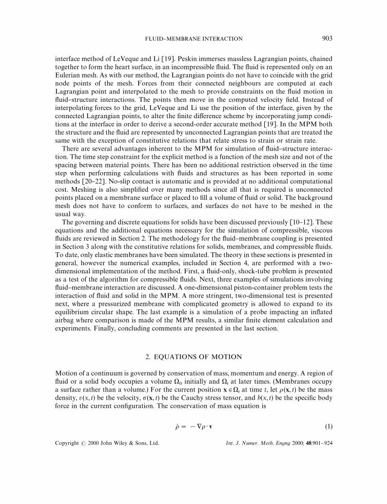
An illustration of the piston-container #uid}structure problem is shown in Figure 7, and theideal MPM representation is shown in Figure 8. Since the problem is one dimensional themembrane does not bend, and thus, resists compression the same manner as it resists tension.



Figure 7. Piston-container problem.

Figure 8. Piston-container MPM simulation set-up.

The interaction between the #uid and structure (spring) occurs only at the single interfacebetween the di!ering materials. At this interface, the #uid and structure stresses contributeinternal forces for the solution of the momentum equation. A similar #uid}structure problem ispresented by Olson [27].

A massless spring of constant K and length ¸ is attached to a piston. The piston can move withoutfriction to compress or expand a compressible #uid of density o and bulk modulus b. The objective isto compare the theoretical frequency of vibration with that from an MPM simulation.

The #uid is assumed to be compressible, inviscid, and adiabatic. The continuity, energy, andconstitutive relations combine to give the relationship between pressure and displacement as follows:

p"!b(+ )U) (26)

where ; is displacement and b is the isentropic bulk modulus. The analytical expression for thenatural frequency, u, of vibration of the mass satis"es the equation

u!J[K#oucA cot (u¸/c)]/m"0 (27)

where c is the wave speed Jb/o, m is the piston mass, and A is the piston cross-sectional area.The parameters used in the MPM simulation are as follows: ¸"20, A"1.0, K"100,

o"0.0001, b"1.58]106, and m variable. The spring is modelled with a linear elastic



Figure 9. Mass (Piston) de#ection in the piston-container simulations.

Table I. Piston-container periods of vibration.

Mass, mTheoreticalu (rad/s)

Theoreticalperiod (s)

MPM simulationperiod (s)

0.1 886.2 0.00709 0.00711.0 281.2 0.02234 0.022

constitutive model so that it also has resistance in compression. The points making up theone-dimensional membrane or spring have a small mass compared to the heavy material point atits end, which has a mass 100 times that of other material points. To determine the frequency ofvibration, the heavy material point representing the piston is given a small initial velocity, and theposition of this material point is monitored.

The "rst solution of Equation (27) gives the fundamental mode of vibration. Table I lists thetheoretical natural frequency and period for two di!erent piston masses along with the periodobserved in the MPM simulation. The observed periods are very close to the theoretical ones.Figure 9 shows the time history of displacement of the mass. The vertical dashed lines in the plotrepresent the theoretical periods of vibration.

4.3. Membrane expansion

A membrane with an arbitrary initial con"guration and a #uid with an initial pressure will evolve,with viscous dissipation, to an equilibrium shape of a sphere or a circle in two dimensions. Here



Table II. Fluid and membrane properties.

Fluid property Value Membrane property Value

Density 1.0 density 0.5Viscosity, k 0.2 Young's modulus 1]106Initial speci"c internal energy, i 250 Poisson's ratio, l 0.3Ratio of speci"c heats, c 1.4Arti"cial viscosity o!

Figure 10. Initial conditions for the dog-bone membrane expansion simulation.

an initial dog-bone shape has been chosen as a severe test for the MPM. The dog-bone-to-cylinder membrane expansion simulation is an arbitrary problem (not seen in the literature) thattests several aspects of #uid}structure interaction. The initial conditions for the problem areshown in Figure 10, and the problem parameters are listed in Table II. A computational elementsize of 0.1 is shown in the "gure; a total of four di!erent element sizes were used.

The problem consists of a gas under internal pressure which expands "lling a cavity that isinitially dog-bone shaped. A membrane forms the cavity and con"nes the gas. At early times, themembrane oscillates due to unbalanced forces. Since the #uid is given a non-zero viscositycoe$cient, the membrane oscillations are damped until a steady-state condition is reached.

There are several areas where this problem can be compared to theory. Some of these are asfollows:

(1) the gas should not escape from the membrane,(2) the equilibrium shape of the membrane should be circular,(3) the stress in the membrane should be consistent with the internal pressure.

Table III lists some of the results of the four simulations that were performed. The simulations aremore re"ned going from 1 to 4 as indicated by the element or mesh size in the second column.Square elements are used. The last two columns show the "nal average pressure and averageradius of the membrane. The "nal radius of the membrane appears to converge with mesh



Table III. Membrane expansion simulation parametersand results.

Simulation element sizeFinal

radius*Final internal

pressure*

1 0.4 1.07 50.32 0.2 1.33 28.83 0.1 1.35 31.24 0.05 1.36 31.7

*Calculated by averaging values at material points.

Table IV. Comparison of hoop stress.

SimulationHoopstress*

Hoop stress-simulations % Di!erence

1 539 101 !81.32 385 399 3.63 420 400 !4.84 443 433 !2.3

*Hoop stress, pr/t, is calculated using the "nal radius and pressure fromTable III with thickness equal to 0.1.sAverage of material point membrane stress.

re"nement as does the "nal internal pressure. The higher "nal pressures of the more re"nedsimulations are consistent with less energy dissipation observed in the plots of the total energy.

Table IV is a comparison of the theoretical hoop stress with the hoop stress observed in thesimulations. The theoretical stress is calculated with the "nal radius and pressure from Table III.There is roughly a 2}5 per cent di!erence between the theoretical value and the simulation value,neglecting the overly coarse simulation. One source of error arises from the fact that the forces arecalculated at grid nodes, and the radius used for the hoop stress calculation in the "rst column isbased on material point locations.

Figures 11}13 illustrate the detailed results of the most coarse and most re"ned membraneexpansion simulations. For each simulation, the material point positions during the initialoscillations are shown along with the shape at steady state. Following this is a plot of themembrane radius as a function of time, measured at 0 and 903 from the horizontal axis, and a plotof the energy.

4.3.1. Simulation 1. Simulation 1 is the coarsest simulation with an element size of 0.4. Figure 11shows the material point locations at increasing times. The simulation is so coarse that the foldsor wrinkles in the membrane cannot be pulled out to a circular shape at equilibrium. However, itcan be seen that gas does not escape the membrane and that the membrane shape does movetoward a circular shape although the circular shape is not achieved.

Time-history plots of the radius at 0 and 903 show that the radii di!er by 0.2 at the steady state,corresponding to the noncircular shape in Figure 11. The time history is also somewhat noisy.



Figure 11. Material point position plots for simulation 1.

Kinetic energy and potential energy for both the #uid and the membrane are also monitored, aswell as the total energy. On the coarse mesh, about 1.5 per cent of the total energy is lost due tonumerical dissipation. The trends observed during mesh re"nement are: (i) the "nal shape of themembrane becomes more circular, (ii) oscillations during the approach to steady state aresmoother, and (iii) there is less energy dissipation.

4.3.2. Simulation 4. Figure 12 shows the material point locations at increasing times for thesimulation with the highest resolution (mesh size 0.05). The "nal time (t"4) is shown larger forclarity. The membrane lines are smooth, and the general shape is approximately the same as inthe simulation with mesh size 0.01 (not shown). The same applies to the radii and energy as seen inFigure 13. There is a 0.03 per cent increase in the total energy during the simulation, and theoscillations in the radii are smooth and are converging to the same value, indicating a "nalcircular shape.

4.4. Airbag impact simulation

Axisymmetric calculations of a cylindrical probe impacting an in#ated airbag were performedand reported by de Coo [28]. The calculations were compared to experimental results.



Figure 12. Material point position plots and pressure contours for simulation 4.

A schematic of the problem is shown in Figure 14. The horizontal axis at the bottom of the "gureis a symmetry axis for cylindrical coordinates. The MPM is used to simulate one of theexperiments reported by de Coo where the diameter, mass, and impact velocity of the cylindricalprobe were varied. The parameters of the simulation are listed in Table V. Material properties forthe simulation are listed in Table VI.



Figure 13. Radii and energy for membrane expansion simulation 4.

Figure 14. Airbag impact problem. Figure 15. Initial con"guration withthe internal tether.



Table V. Airbag impact simulation parameters.

Cylinder (probe)diameter (mm)

Cylindermass (kg)

Cylinder initialvelocity (m/s)

200 6.03 3.90

Table VI. Airbag impact simulation*material properties.

Airbag property Value Air property Value

Thickness 0.5 mm Speci"c heat ratio 1.4Density 662 kg/m3 Density 1.2156 kg/m3Young's modulus 6]107 N/m2 Initial pressure 4000 N/m2Poisson's ratio 0.4 Initial speci"c internal energy 8226 J/kg

Material properties of the cylinder were not listed. Therefore, Young's modulus was arbitrarilychosen to be 5]107 N/m2, and the density was adjusted to give the correct mass. The total airbagmass was derived to be 367.2 g.

The initial positions of the membrane material points for this simulation were arrived at byconducting a simulation with a tether in the airbag. The initial positions of the material points areshown in Figure 15. This con"guration was allowed to come to approximate equilibrium and theresulting airbag shape was used as the initial shape for the simulation of the probe impact. Theobjective of this exercise was to obtain an initial shape that matches that reported by de Coo.

The plots of the probe and airbag material point positions for various times during thesimulation are shown in Figure 16. The e!ect of using the tether to determine initial materialpoint positions is seen in the "rst plot of Figure 16. The tether pulled the material to the left(indicated by the arrow in the top left plot).

For the simulation with the probe, the tether was removed at the instant the simulation wasstarted because in the axisymmetric MPM calculation this tether is actually a conical shape anda!ects the #ow of the gas material points. There were approximately 3000 material pointsrepresenting the gas. These are not shown in Figure 16 to increase the clarity of the airbag shape.The predicted con"guration of the airbag and impactor look plausible. As the impactor moves tothe left, it depresses the airbag, causing the airbag to bulge out in response. The probe slows afterimpact, eventually stops and then rebounds to the right.

Figure 17 shows a comparison of the displacement of the probe into the airbag for the MPMsimulation, the PISCES simulation and the experiment [28]. Figure 18 shows that the deformedairbag shapes at t"40 ms are similar. The slope of the displacement past the peak in Figure 17di!ers from that displayed by the experimental data. It is thought that the e!ect of not simulatingthe tether may cause a more rapid rebound of the impactor since the airbag expansion is notrestrained. To test this theory, a simulation was conducted where the tether was left in thesimulation for the duration. It was observed that the slope past the peak closely matched that ofthe experiment, which did incorporate a tether. However, the cylinder displaced about 20 mmfarther into the airbag. This excessive displacement is attributed to the interference of the tetherwith the gas #ow.



Figure 16. Deformed airbag shapes.

An alternative to modelling the tether with material points would be to prescribe a force}displacement relationship between two material points. The force}displacement relationshipcould be that of a spring or bar to represent the tether, but in general could take any form. Thisforce would be interpolated to the grid at the two particle locations and included as an external



Figure 17. Displacement results forthe cylindrical probe.

Figure 18. Comparison of PISCES and MPMdeformed con"guration for t"40 ms.

force in the solution. In principle, this method would be equivalent to that described above, butwould have the advantage of not interfering with the gas particles.

5. CONCLUSIONS

The material point method uses Lagrangian material points and an Eulerian or spatial mesh tode"ne the computational domain.The material points move through the Eulerian mesh, on whichthe momentum equation is solved. A review of the equations is given as they are developed forgeneral solid materials, membranes and compressible #uids. This paper presents the modi"ca-tions necessary to simulate the interaction of thin membranes and compressible #uids.

Several test problems are presented to demonstrate the methodology. A #uid-only shock tubeproblem is used to test the compressible #uid model, and a one-dimensional piston-containerproblem validates the implementation of #uid}membrane interactions. Both of these problemshave analytical solutions that are used for comparison with the numerical results. Two morecomplex simulations of a gas-"lled pressurized membrane and of a probe impacting a pre-in#atedairbag show the potential of the method. These last two problems are two dimensional andinvolve complicated geometry that is easily represented by the material points. In addition, theairbag problem has also been solved using "nite elements and experimental measurements havebeen made, both of which compare well with the MPM results.

The treatment of the interface between the #uid and membrane is simple in the MPM andavoids the time-consuming computations necessary in many methods. One major advantage tothis approach is that meshing bodies is trivial. Since points only have to be identi"ed that areinside a body or on membrane surface, the potentially expensive process of meshing with



standard "nite elements is avoided. Other advantages are that the constitutive equations areeasily changed, and the algorithm runs on a PC or workstation, but can be easily parallelized formore powerful machines and larger problems.

ACKNOWLEDGEMENTS

This work was partially supported by Sandia National Laboratories. Sandia is a multiprogram laboratoryoperated by Sandia Corporation, a Lockheed Martin Company, for the United States Department ofEnergy under Contract DE-AC04-94AL85000.

REFERENCES

1. McMaster WH. Computer codes for #uid-structure interactions. Proceedings 1984 Pressure <essel and PipingConference, San Antonio, TX, June 1984, ;CR¸-89724 preprint, Lawrence Livermore National Laboratory, 1984.

2. Buijk AJ, Low TC. Signi"cance of gas dynamics in airbag simulations. Presented at the 26th ISA¹A, Aachen,Germany, September 1993.

3. Buijk AJ, Florie CJL. In#ation of folded driver and passenger airbags. Presented at the 1991 MSC =orld ;sersConference, Paper 91-04-B, Los Angeles, California, March 1991.

4. Koivurova H, Pramila A. Nonlinear vibration of axially moving membrane by "nite element method. ComputationalMechanics 1997; 20:573}581.

5. Nieboer JJ, Wismans J, de Coo PJA. Airbag modeling techniques. Proceedings of the 34th Stapp Car CrashConference, SAE Paper 902322, 1990.

6. Liu WK, Ma DC. Computer implementation aspects for #uid}structure interaction problems. Computer Methods inApplied Mechanics and Engineering 1981; 31:129}148.

7. Nomura T. ALE "nite element calculations of #uid-structure interaction problems. Computer Methods in AppliedMechanics 1994; 112:291}308.

8. Brackbill JU, Ruppel HM. FLIP: a method for adoptively zoned, particle-in-cell calculations in two dimensions.Journal of Computational Physics 1986; 65:314}343.

9. Brackbill JU, Kothe DB, Ruppel HM. FLIP: a low-dissipation, particle-in-cell method for #uid #ow. ComputerPhysics Communications 1988; 48:25}38.

10. Sulsky D, Chen Z, Schreyer HL. A particle method for history-dependent materials. Computer Methods in AppliedMechanics and Engineering 1994; 118:179}196.

11. Sulsky D, Zhou S-J, Schreyer HL. Application of a particle-in-cell method to solid mechanics. Computer PhysicsCommunications 1995; 87:136}252.

12. Sulsky D, Schreyer HL. Axisymmetric form of the material point method with applications to upsetting and Taylorimpact problems. Computer Methods in Applied Mechanics and Engineering 1996; 139:409}429.

13. York AR, Sulsky DL, Schreyer HL. The material point method for simulation of thin membranes. InternationalJournal for Numerical Methods in Engineering 1999; 44:1429}1456.

14. Huerta A, Liu WK. Large-amplitude sloshing with submerged blocks. Journal of Pressure <essel ¹echnology 1990;112:104-1-8.

15. Thematic Issue on Particle Simulation Methods, Computer Physics Communications 1995; 87(1}2).16. Special Issue on Meshless Methods, Computer Methods in Applied Mechanics and Engineering 1996; 139(1}4).17. Peskin CS. Numerical analysis of blood #ow in the heart. Journal of Computational Physics 1977; 25:220}252.18. Peskin CS, McQueen DM. A general method for the computer simulation of biological systems interacting with#uids. Symposium-Society for Experimental Biology, U.K., ISSN/ISBN 0081-1386, 1995.

19. LeVeque RJ, Li Z. Immersed interface methods for Stokes #ow with elastic boundaries or surface tension. SIAMJournal on Scienti,c Computing 1997; 18:709}735.

20. Jones AV. Fluid-structure coupling in Lagrange}Lagrange and Euler}Lagrange descriptions. Report E;R 7424 EN,Nuclear Science and Technology, Commission of the European Communities, Joint Research Centre, Ispra Establish-ment, Italy, 1981.

21. Neishlos H, Israeli M, Kivity Y. Stability of some explicit di!erence schemes for #uid}structure interaction problems.Computers and Structures 1981; 13:97}101.

22. Neishlos H, Israeli M, Kivity Y. The stability of explicit di!erence schemes for solving the problem of interactionbetween a compressible #uid and an elastic shell. Computer Methods in Applied Mechanics and Engineering 1983;41:129}143.

23. Burgess D, Sulsky D, Brackbill JU. Mass matrix formulation of the FLIP particle-in-cell method. Journal ofComputational Physics 1992; 103:1}15.



24. Bardenhagen SG, Brackbill JU, Sulsky DL. The material-point method for granular material. Computer Methods inApplied Mechanics and Engineering 1999; to appear.

25. Wilkins ML. Use of arti"cial viscosity in multidimensional #uid dynamic calculations. Journal of ComputationalPhysics 1980; 36:281}303.

26. Sod GA. A survey of several "nite di!erence methods for systems of nonlinear hyperbolic conservation laws. Journalof Computational Physics 1978; 27:1}31.

27. Olson LG, Bathe K. A study of displacement-based #uid "nite elements for calculating frequencies of #uid and#uid}structure systems. Nuclear Engineering and Design 1983; 76:137}151.

28. de Coo PJA, Nieboer JJ, Wismans J. Computer simulation of driver airbag contact with rigid body. ¹NO Report No.751960020 to M<MA, December 1989.



Documents

Fluid membrane interaction based on the material point …sulsky/papers/IJNME2.pdfFluid-membrane systems are quite common and include parachutes, ... externalforcesare problem speci"candare