Embed Size (px)
Citation preview

Fluid Space Theory
“I Reject Your Physics and Substitute My Own” Copyright 2017, John S. Huenefeld. All rights reserved.
By John S. Huenefeld
Abstract
This web site is to propose that gravity is the manifestation of fluid motions in a
four dimensional space-time-energy continuum. The reasons for this arise from
philosophical and technical problems with today’s accepted mainstream theory.
First of all, the fact that Dark Energy, and Dark Matter must be invented out of
nowhere to make the standard model match observations is a huge red flag that our
understanding is fundamentally wrong. Second, the separation of matter-energy
from space-time in Einstein’s form of General Relativity (GR) precludes exploration
of energized space-time which is the key to truly understanding our cosmos. To
follow this explanation of Fluid Space Theory, the reader must have a good
knowledge of modern physics, including Einstein’s Special Theory of Relativity and
a basic understanding of what General Relativity is.
I will not use tensor notation in any of my derivations. I freely admit that when
I look at a tensor equation I get no mental picture of what is going on inside the
mathematics. Einstein himself lamented the circumstance whereby progress in
physics was attained by increasing dependence on abstract mathematics, putting a
greater distance between the theorist and experimental observations of physical
phenomena. For example, Maxwell’s equations for electromagnetism were first
written as differential equations, they were only generalized more recently. Full
generalization is not actually better in conveying meaning. A generalized rhetorical
question might be phrased “Do fauna deposit waste among flora?” While very clean,
compact, and general, it lacks all the character and meaning of the original “Does a
bear crap in the woods?” So, in the spirit of Maxwell, I will stick to specific
equations with specific meaning.
About equations. Math is the language of physics. If you are reading this you
must be interested in learning about physics. Learning the math is key to truly
understanding physics, so a student of physics should not shy away from equations.
Would you want to learn about China, Japan, or Mexico from books that strictly
avoided using Chinese, Japanese, or Spanish words? In fact, it would be best to
learn about those countries in the language of those countries. I will therefore use
equations without apology.
So, what does Fluid Space Theory do, and how is it different from Einstein’s
general relativity? The following lists show the what and the how, the following
pages explain the why.

What Fluid Space Theory does:
1. FST replicates Newtonian gravity, from small radii out to infinity.
2. FST replicates curved space and time dilation of Einstein’s general relativity.
3. FST reveals an undiscovered space-time contraction field around matter which
replicates the effects currently attributed to dark matter and dark energy.
4. FST eliminates the troublesome singularity inside a black hole and transitions
seamlessly into quantum theory.
How Fluid Space Theory is different from Einstein’s general relativity:
1. FST is simple and easy to understand. Nothing more than differential equations
is required, no tensor calculus is needed (unless you really want to use it).
2. FST recognizes the existence of relative velocity fields in space-time, fields that
Einstein should not have dismissed.
3. FST has none of the mysticism of general relativity. It makes curved space-time
easy to visualize.
4. FST unites matter and space-time into a single entity. No more “matter tells
space-time how to curve and space-time tells matter how to move.” In FST, matter
is curved space-time and it tells itself how to move.
The 2 Rules for Implementing Fluid Space Theory
1. Fluid Space Theory always works.
2. If Fluid Space Theory does not work, you are doing something wrong; refer to
rule number 1.
After working with Fluid Space Theory for so long, I decided to move these rules
to the front. Time and time again when I thought I was at a dead end, going back
and taking a closer look, thinking it through more carefully, lead me to a new
answer and a new discovery. Fluid Space Theory has never failed to hold up. These
rules are no joke.
Section 1: The Football Analogy
The first time I recall thinking about Fluid Space Theory was around age 16
while throwing a football (American football) around in the yard. I had recently
begun studying Newton’s laws and imagined that if the football field was out in
space, when I threw the ball it would continue in a straight line and constant
velocity and I would never get it back. In order to make the ball arc back to the
ground, the field would need to have rockets, which when fired would create
artificial gravity. In the Newtonian perspective, the football would continue in a
straight line but the field would accelerate toward it through space, eventually
catching up when the football would “hit the ground.” In reality, it is the ground, or
field which hits the football.
I then tried to bring the Newtonian analogy to the surface of the Earth. I
reasoned that if the football field had to accelerate through space to catch up with

the football, something similar might be going on with gravity. I didn’t know it at
the time but I was trying to apply Albert Einstein’s principle of equivalence (more
about that later).
I thought that in order to make the football fall back down, space would have to
be accelerating through the surface of the Earth. I was pretty excited about my
cleverness and thought I might be onto something until it occurred to me that the
Earth is round, and since gravity is the same everywhere, space would have to be
passing through the earth’s surface everywhere, all the way around, but where
would it go? I concluded, like many before me, that this was a silly idea and the
analogy was flawed. But the thought continued to nag at me as a problem that
needed to be solved.
I am happy to report that I have in fact solved the problem, and the process of
solving it has revealed several fallacies incorporated as truths in modern physics
and additional blunders that Albert Einstein made.
I would like to begin with a quick review of Isaac Newton’s laws of motion,
which I would rather call his “laws of space”, because they tell us how things relate
to space. I will not cite any references, just do a web search for them and you will
find many places and phrasings from which you can choose.
1. An object in a state of uniform motion will remain in that state of motion until acted upon by an external force. An object at rest will remain at rest until acted upon by an external force.
2. The change in the state of motion of an object acted upon by an external force
is directly proportional to the magnitude of the acting force and inversely proportional to the mass of the object. (acceleration a=f/m or force f=ma).
3. For every action there is an equal and opposite reaction.
These three laws gave birth to the industrial revolution and are the basis of all
our modern mechanical devices from skateboards to satellites and everything in
between. It is truly amazing how powerful three simple and correct statements
which illustrate a true understanding of nature can be.
Fluid Space Theory is based on considering space as something real, as a
definable stage upon which objects and forces may act. There is nothing inherently
wrong about thinking of space in this way. There are however, many scientific
observations which require an increasingly sophisticated concept of space in order
to be explained, but fear not, Fluid Space Theory is up to the task. In terms of Fluid
Space Theory, Newton’s laws tells us the following:
FST 1. Objects move through space without resistance, and conversely space moves through objects without resistance. An object will not change its relationship

with its spatial reference frame unless acted on by an external force.
FST 2. An object acted upon by an external force will change its relationship with its resting spatial reference frame in direct proportion to the magnitude of the force and inverse proportion to the mass of the object. (a= f/m or f=ma).
FST 3. In order to change the relationship of an object to its resting spatial reference frame, the acting object must change its relationship with its resting spatial reference frame in equal proportion.
In short, where Isaac Newton saw forces acting between material bodies, Fluid
Space Theory sees reference frames in motion and material bodies changing their
relationships with those reference frames. Now we can revisit our rocket powered
football field and attempt to bring it down to Earth.
It is an unwritten rule in any sport you can name that it must be played in 1
Earth normal gravity or 1G. The sizes of the fields and goals, the size and masses
of the balls, and the inflation pressures are all tailored to normal Earth gravity. If
played under different gravity, the game would not be the same at all. Imagine
playing basketball on the Moon, even a fourth grader would be able to do a slam
dunk or take a shot from anywhere on the court. It would be a completely different
game. So our space football field must have rockets strong enough to accelerate at 1
Earth normal gravity or 1G to play Earth football.
Lets imagine a rocket powered football field out in space and also imagine that
the players are robots so we don’t have to worry about having an atmosphere or
using a space suit. It is a practice field, so to conserve fuel, the rockets are turned
off between plays. Also to keep the field small, it ends at the out of bounds lines
and the coaches and trainers float nearby equipped with rocket packs of their own
so they can keep up.
Figure 1-1.

For the first play, lets imagine that the rockets never come on. In this situation,
when the quarterback throws the ball it will fly in a straight line up and away from
the field at a constant velocity and one of the trainers with a rocket pack will have
to fly out and retrieve it. . See figure 1-1.
For the next play, lets imagine that a coach is floating about 40 yards above the
field so he can watch from above. The ball is snapped, the field thrust rockets fire,
and gravity appears on the field, the quarterback fades back and throws the ball to
a receiver running down the sideline. The receiver outpaces the defender, makes a
catch and runs into the end zone for the score. The play is over, the rockets turn off
and gravity on the field goes away. This all happens before the field passes the
coach who has not fired his rocket pack. Let’s take a look at what the floating coach
sees from his point of view. See figure 1-2.
Figure 1-2.
The coach floating above will see the play start and the field begin to accelerate
toward him. When the ball is thrown, he will see it travel in a straight line at a
constant velocity just like it did last time. The ball will fly up above the field until
the field catches up and lifts the receiver into position to intercept the path of the
football and make the catch. Once the play is over, the coach will see the field fly
past and will have to use his rockets to match velocity.
To the players on the field, the field remains stationary and the ball flies in a
arc as shown on the top of figure 1-2. So why does the floating coach see the ball
trace a straight line while players on the field see it travel in a arc? To see how this
works we can use Newton’s first two laws and a little math to draw figure 1-3.

An equation representing a football at rest is simply its position relative to some
arbitrary starting point along a horizontal axis we will call the yard line. I use the
subscript 0 to indicate the position of the ball at time t=0. This is a pretty boring
example because x sub zero never changes. It is what we see when the official
places the ball on a yard line and we wait for the next play to start.
Next, let’s give the football a constant velocity toward the opposing goal line.
The position of the football will now change at a constant rate so the position can be
calculated by multiplying the velocity by the amount of time that passes.
So far we have only used Newton’s first law. It is time to employ the second
law. If the mass of our the football is constant and the force applied to it is
constant, the acceleration will also be constant. We can write the following
equation to find the yard line of the football if a force is applied to it.
Let’s say that while floating in weightlessness above our outer space football
field, a small rocket is attached to the football that will accelerate it at 2 yards per
second each second toward the opposing goal line and that it is above the 5 yard line
moving 2 yards per second toward the opposing goal line when the rocket fires. The
equation becomes as follows once we plug in the values for a, v zero, and x zero.
Just plug the amount of time since the clock is started into the equation and you
can find the yard line the football will be at. This is great for one dimension, but
football is played in space and space has three dimensions. The football can not
only move back and forth between the goal lines, it can move sideways and up and
down as well. Traditionally these directions are labeled x, y, and z. We can use x
for the direction between goals, y for the direction side to side and z for the direction
up and down. Now we just use three identical equations, one for each direction and
plug in the values for acceleration, velocity, and position that apply in each
direction.
We can simplify the math by setting the starting point of the throw as yard line
zero (x sub zero becomes zero). We can also have the quarterback throw the ball
straight down field so we don’t have to bother with the side to side, or y direction
motion at all (y velocity is zero). Also, knowing that the rockets attached to the field
are pointed straight down, we will only have to deal with acceleration in the z

direction ( ax and ay are zero).
Let’s say that in the pass play, the quarterback throws the ball sixty yards and
it takes six seconds to get there, so the velocity down field in the x direction is ten
yards per second. Now, to make the math easy let’s say the field rockets increase
the upward velocity of the football field at two yards per second each second (Earth
gravity is more like 10 yards per second each second but using 2 makes the math
easier). let’s also say that the quarterback gives the football an upward velocity of
six yards per second. Figure 1-3 is a chart of what the coach above the field sees by
remaining stationary relative to the Newtonian reference system at the start of the
play and we can write the following equation for the position of the ball and field
during the play.
We can plot the path of the ball on a graph as in figure 1-1 and see that the ball
travels in a straight line moving up six yards and downfield ten yards each second.
We can also plot the position of the field showing that it will be 1 yard above its
starting point at 1 second, 4 yards at 2 seconds, 9 yards at 3 seconds, 16 at 4, 25 at 5
and 36 at 6, and we see that the field catches up to the ball at six seconds when the
ball is sixty yards down field.
Figure 1-3.

To see what the players on the field see, take another piece of graph paper and
lay it over the top of figure 1-1. For each second, move the field level z=0 line up to
the position of the field and mark the position of the ball for that second. When
finished you will see that the points form a curve as show in figure 1-3.
This is what I was thinking about on that day throwing the football around in
my yard. The instant the football is thrown, it enters a state of freefall. If you were
riding on it, you would feel weightless, just like an astronaut in space. Out in space,
with a rocket powered field, the ball actually travels in a straight line and the field
accelerates upward to catch up with it. If gravity as felt on a rocket powered
football field in space is the same as gravity felt on the Earth, then space has to be
imagined as accelerating downward through the surface of the Earth. This is a
problem for a lot of people, because a lot of space would have to vanish, and rather
than solve that problem, they will say “you just shouldn’t think about space that
way”. I can think about it that way, and I do think about it that way, and I have
solved the problem of the vanishing space!
Before going on I want to show that it is possible to see both points of view
either from in space with a rocket powered field or on the surface of a planet.
Seeing the point of view from the field in Figure 1-3 is easy, you just stand on the
sideline of the practice field and watch. Seeing the field as the floating coach did in
figure 1-3 takes a little more work.
Figure 1-4.

While floating in space with no rockets firing, you are in the condition of
Newton’s first law, or otherwise known as freefall. In order to experience this on
the surface of a planet you must jump from a tower or airplane or otherwise be
launched into the air, and for a while as you fall, before air resistance builds up, you
will experience weightlessness or freefall.
To view the play from a Newtonian freefall reference frame, the coach must
jump from a tower above the field at the moment the ball is thrown. If the planet
has gravitational acceleration of 2 yards per second each second, he will be 1 yard
lower after the first second, 4 lower after second number two, 9 after the third, etc.
He will fall the same as the field rose in the outer space example. See Figure 1-4.
Now if you take a sheet of graph paper and lay it over figure 1-4 with the coach
starting 36 yards above the field and mark the position of the ball at t equals zero,
and then move the sheet down to put the coach where he would be at the end of
each second and mark the position of the ball as it travels through its arc, you will
see that from the coach’s point of view, the ball moves in a straight line at a
constant velocity. In case you were worried, there is a giant air pillow for the coach
to land on.
From a Newtonian point of view both cases work either out in space or on the
surface of a planet. It cannot be denied that on a planet with gravity, inertial
reference frames are constantly falling through the surface. All you have to do is
drop or throw something to see it in action. Somehow, the Earth is gobbling up
falling reference frames. How can this be happening? In the next section I will take
a more structured and mathematical look at what is going on.
Section 2: The Case for Spatial Flows
In cosmology, the concept of universal expansion is widely accepted. In this
theory, the fabric of space-time expands, carrying galaxies outward like raisins in a
rising loaf of bread. At any given position inside this space-time an invisible
expansion field may be imagined as spheres of space-time moving outward with a
velocity increasing in proportion to the distance from any chosen central point. This
is a widely accepted and easily understood example of a space-time velocity field.
There is another somewhat accepted velocity field. In the description of what is
happening at the event horizon of a black hole, the waterfall analogy is commonly
used. In this analogy, space-time is said to be falling into the black hole at the
speed of light. Like a swimmer upstream of a waterfall, anything caught in this
flow will be swept down into the black hole never to return. This will happen even
while swimming at top speed (which in this case is the speed of light). Once again,
an accepted concept of a space-time velocity field and not much different than my
football analogy.
There is, however, a problem with the waterfall analogy which is subsequently
ignored. If space-time is flowing into the black hole at the speed of light at the
event horizon, it must also be flowing into a concentric sphere just outside of the
event horizon at a velocity just under the speed of light. In fact this may be
imagined to go on through increasingly larger spheres at lower velocities on out to
infinity. Also, if this is true of black holes, why would it not be true for neutron
stars, or normal stars, or large planets or any gravitating body? Gravity is gravity
whether generated by a black hole or any other massive body. If the waterfall
analogy applies to black holes it must also apply to stars and planets, even atoms.
It then logically follows that all objects with the property of mass must be
surrounded by an inward velocity flow field.
This is a problem, and a line of thinking that physics professors have been
steering students away from since the time of Einstein. I ask the reader to indulge
me and follow this line of reasoning, as I characterize these inward velocity fields.
The first step is to establish the concept of space-time flux.
Let us begin with flat space-time known in General Relativity (GR) as
Minkowski space. In the tradition of Albert Einstein's thought experiments, let us
travel in mind to a region far from any massive bodies, where there are no energetic
fields, where parallel lines never meet, and an object left alone will travel forever in
a straight line at a constant velocity. Let us imagine a glass box measuring several
meters on a side in this space. Inside the box are several objects and a human
observer. A human observer is posted outside the box as well. At present, all these
items float weightless and motionless (see fig 2-1A).

Figure 2-1.
Inertial and accelerated systems.
While weightless, these objects could be traveling through space-time at any
velocity from zero to c (the speed of light). They would have no way to tell what that
velocity is, but whatever it is, they can tell it is not changing (Newton’s or FST first
law). We could then say that the velocity field, or space-time flux, (the amount of
space-time passing through the box) is constant. If we discard any unknown
background velocity, using the cross sectional area of the box we can compute the
relative flow of space-time through the box. We don‘t know an absolute flux, but a
relative flux can be described by equation (1). The volume flux will have units of
meters cubed per second, m3s-1. All further references on this website to space-time
flux may be considered as “relative flux.”
(1)
In Figure 2-1B, a force has been applied to the top of the box and now the
observer inside the box experiences an increasing space-time flux. Space is flowing
through the box at a constantly increasing rate and she experiences gravity. The
change in space-time flux with time can be expressed by equation (2). The change
in space-time flux will have units of m3 s-2, and these are the units that describe
accelerated flow and produce the sensation of gravity.
(2)
Understanding that acceleration (a) is the time derivative of velocity this
equation may be rewritten as equation (3).
(3)
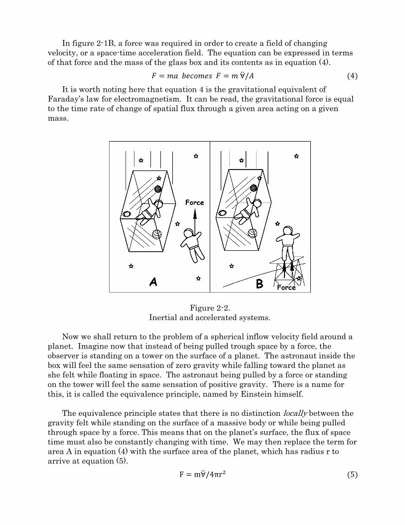
In figure 2-1B, a force was required in order to create a field of changing
velocity, or a space-time acceleration field. The equation can be expressed in terms
of that force and the mass of the glass box and its contents as in equation (4).
(4)
It is worth noting here that equation 4 is the gravitational equivalent of
Faraday’s law for electromagnetism. It can be read, the gravitational force is equal
to the time rate of change of spatial flux through a given area acting on a given
mass.
Figure 2-2.
Inertial and accelerated systems.
Now we shall return to the problem of a spherical inflow velocity field around a
planet. Imagine now that instead of being pulled trough space by a force, the
observer is standing on a tower on the surface of a planet. The astronaut inside the
box will feel the same sensation of zero gravity while falling toward the planet as
she felt while floating in space. The astronaut being pulled by a force or standing
on the tower will feel the same sensation of positive gravity. There is a name for
this, it is called the equivalence principle, named by Einstein himself.
The equivalence principle states that there is no distinction locally between the
gravity felt while standing on the surface of a massive body or while being pulled
through space by a force. This means that on the planet’s surface, the flux of space
time must also be constantly changing with time. We may then replace the term for
area A in equation (4) with the surface area of the planet, which has radius r to
arrive at equation (5).
(5)

While the observer is sitting on the surface of the planet, the force of gravity felt
remains constant. This is also true for the observer being pulled through space by a
constant force. Looking at the term V double dot, we see it has units of m3s-2 This
is very similar to the units of the gravitational constant G which has units m3kg-1s-2.
If V double dot is assumed to be proportional to the mass M of the planet, we may
replace the change in space-time flux term, V double dot, with a convenient
constant, 4 pi G, which is applied in proportion to the mass M of the planet and we
get the very familiar equation (6).
(6)
In this way, Newton’s equation for gravity may be derived on the basis of a
space-time inflow velocity field. Of course, there is a problem with this. If space-
time is flowing into the planet from all sides, where is it going? The planet should
quickly fill up with space-time and the flow will come to a stop. Also, it would seem
that the flow velocity at the surface would have to be constantly increasing with
time to create gravity, making the situation even worse. The amount of space-time
volume passing through any imagined sphere at radius r must be accounted for, as
well as the second order term for ever increasing velocity, and this seems
impossible.
At this point, most people have thrown up their hands and walked away from
this line of thinking, but not me. There is an answer, and it is precisely by
accounting for this “lost volume” of space-time, that the cause of galaxy rotations
faster than predicted by Newton’s gravitation equation (dark matter), and changes
in the observed rate of expansion of the universe (dark energy) can be explained.
2.2: Sink flows and acceleration fields.
This section will show and explain how gravity is created by space time flux in a
sink flow field. To begin with we need to understand space-time flux, or any kind of
flux for that matter.
Figure 2-3 shows four pipes of equal area and length. If a fluid of any kind
flows down these pipes at velocity v, the flux will be the same in all the pipes, and it
will be equal to the velocity of the flow times the area of the tube. Flux has the
dimensions of length cubed per second.
If the tubes are fitted with tapering ends, while the inlet area of each tube is the
same, the area of the outlet is smallest for the top tube and largest for the bottom
tube. If the flux is the same down each tube, the velocity of the fluid when exiting
any tube will be higher than it was upon entering. This is known as a nozzle, and is
used to accelerate fluid flows. The smaller the exit, the higher the velocity. The
tube at the top will have the highest exit velocity. If you know the amount of flux
(flow volume per second) and the area of the exit, the velocity can be easily
calculated.

Figure 2-3
Figure 2-4
Let’s take a closer look at the tapered section of a tube. In a straight section of
tube with a constant area, the velocity remains constant. For space-time flux this
represents an inertial reference system. It is only in the tapered section of the tube
where the area is changing that the velocity is also changing. Changing velocity is
known as acceleration. Within the tapered section an acceleration field exists
within the fluid flow. In Fluid Space Theory, an acceleration field of space-time flux
represents an accelerated reference frame or a gravity field.
Going back to the astronaut in the glass box of figure 2-1A, it is as if she is in
one of the constant area pipes where space-time is moving past at a constant

velocity. When the cable attached to the box is pulled, as in figure 2-1 B, it is like
moving her to an area where the flow velocity of space-time is constantly changing.
From her point of view, it is placing her into an acceleration field within space-time.
This can be imagined as either increasing the flow velocity at a steady rate down a
straight section of pipe, or by moving her into a tapered section of pipe with a
constant space-time flux.
FST law number 1 says that space flows through objects without resistance. So
there is no material pipe that can contain or funnel a flow of space-time. The only
thing that can resist the passage of space-time is other space-time. If space-time
could be magically removed inside a small sphere, the surrounding space-time
would rush in to replace it. If this is kept up on a continuing basis, a self funneling
inflow field will form.
In the study of fluids, a flow field that originates from, or converges into, a
central point is called source or sink flow. If one of the tapered sections of pipe is
separated from the straight pipe sections and then packed in with a bunch of other
tapered pipes around a central point, it can seen how sink flow is no different from
flow in a tapered pipe. See figure 2-5.
Figure 2-5
So in figure 2-2B, while the astronaut is standing on the tower, above the
planet, he is standing in a tapered flow field, or acceleration zone, also known as a
gravity field. (Remember, in Fluid Space Theory, an acceleration field in space-time
is a gravitational field.)
So at least a part of the mystery of the vanishing space-time has now been
solved. By visualizing sink flow of space-time into the Earth, the flow can be in a
steady state, the flux at any radius can be constant over time. There is no need for
an increasing amount of flux to create gravity as in figure 2-1 B. The taper of the
flow creates the acceleration field, so while standing in this field we feel gravity
even though the space-time flux is constant.

Section 3: Application of Relativity to Spatial Flows
Einstein’s theories of relativity are based on the four dimensional nature of
space-time. In our normal understanding of length in three dimensions, we can find
the distance between any two points given their coordinates using the Pythagorean
theorem.
To introduce the fourth dimension of time, the first thing that must be done is
to express time in units of length so we use the term tc ( time multiplied by the
speed of light) which has units of length.
The Pythagorean theorem works with any number of dimensions and in this
case we are using a four dimensional axis, x, y, z, and tc, each axis is perpendicular
to all the others. You may have noticed that the tc term is subtracted rather than
added. This is done to make the calculated space-time intervals match
observations. So not only is the tc axis perpendicular to x, y, and z, but distances
along it are measured in reverse.
This is where the Lorentz transformations Albert Einstein used in his special
theory of relativity come from. Time and space, said Einstein, are not the rigid and
inflexible things that Newton thought them to be. Time does not pass at the same
rate in all references frames, nor are distances the same in all reference frames. He
gave us the equations below that can be used to predict the rate of time and the
lengths of objects based on their relative velocities. These equations will be
valuable in applying relativity theory to spatial flows.
By understanding that lengths perpendicular to the direction of motion are not
contracted, we can write an equation for the volume V of an object as it approaches
the speed of light. Where V equals length times width times height and V prime
equals length prime times width times height.
(7)
Variables marked prime (l') are those in the moving reference frame while
unmarked variables are in the reference system of the observer. Above, the letter l
stands for length and t means time and means volume, v is the relative velocity of
the moving reference frame and c is the speed of light. If the prime and normal
quantities are known for both reference systems the equations may be inverted to
solve for the relative velocity as shown below.
Equation 7 tells us that the observed volume of an object in relative motion is
less than the volume of that same object when at rest. So how exactly does an
object change when accelerated to a high relative velocity?
Let us consider what we know of “tangible objects”. If we say that an object is
“moving through space,” we may also be saying that space is “moving through the
object.” We know that ordinary objects are composed of tiny molecules arrayed in
space, that those are in turn composed of even smaller atoms, and that there is
space between them. Thanks to the work of Rutherford and Bohr, we also know that
atoms are themselves mostly empty space where tiny fuzzy electrons whirl about a
dense and tiny nucleus. This nucleus is in turn occupied by a host of even smaller
fuzzy things (protons and neutrons), and there is space between them. They are in
turn composed of even smaller fuzzier things, and there is space between those
(quarks or strings).
Thus, an ordinary object would present no greater impediment to the passage of
space than the planets would prevent space from passing through our solar system.
Objects that we perceive as solid are actually, almost completely made up of empty
space, it is only the fields surrounding these very tiny particles that makes them
seem solid. When we use the equations of special relativity to compute contraction
of the length of an object traveling near the speed of light, we are actually
computing the changes in the space the object occupies, not the object itself.
Specifically, the coordinate axis in a moving reference frame, aligned in the
direction of motion, will appear to be compressed to an observer in another
reference frame. Any object placed into that moving reference frame will also
appear compressed along that axis. So it is the space that is changing, not the
object. Therefore in the study of sink flows of space-time we must understand that
the 3 dimensional volume of the flow will change based on the velocity of the flow.
3D volume is not conserved under a velocity transform.
Now let’s return to the notion of space-time falling through the surface of our
imaginary planet. As the inertial reference frame falls inward, it moves faster and
faster. The faster it moves, the shorter it becomes in the direction of motion (the
radial direction), and its internal volume decreases. When it reaches the speed of
light, its volume will vanish entirely. At this point, space-time may continue to fall
endlessly inward without ever getting any closer to the central point. This is called

the event horizon and space-time beyond this horizon is bent so much that it may be
imagined as flowing off perpendicularly to our universe. In this context, the notion
of space-time flowing into matter is not so absurd after all. The inflow of space-time
vanishes as it becomes compressed with velocity and eventually all length in the
direction of motion is shifted over to the tc axis.
Before developing the mathematics of an inflow field I must establish a couple
of conventions. First vectors are defined as positive outward and negative inward
toward the central point. Second, I will be careful using the radius of a sphere in
the equations because with spatial compression in the radial direction, using the
radius can lead to some confusion. Finally when applying relativity to the flow
field, one must consider both the view of an observer greatly removed on the outside
of the flow and the view of an element traveling within the flow field. These two
views can become very different. From equations 4 and 6 we can establish that
a=f/m and come up with the following.
First we set the acceleration equal to the time rate change of velocity
Next by applying the chain rule we look for the velocity change with respect to
the radius, realizing that the time change in radius of a falling shell, dr/dt is equal
to v. We may now solve for dv/dr.
Integrating both sides we get.
(8)
We recognize this equation as the Newtonian formula for escape velocity from a
gravitating body. In this case, we are not considering a body falling through
Newtonian space but space-time itself falling toward a central point. It is not only
the velocity required to escape from a given radius, but also the velocity that would
result by falling from a standstill at an infinite radius. At any radius in a
gravitational field, space-time falls inward or outward at escape velocity.

The velocity of the flow field must be adjusted for the effects of relativity as
would be seen by an observer outside the flow field. Applying the equations of
Special Relativity from above, to correct for both spatial compression and time
dilation we get.
(9)
Figure 3-1 is a plot of flow velocity as a function of the radius. In this graph v is
the Newtonian form of an element of space-time fluid within the flow and v prime is
how the velocity of this same element would appear to an observer outside the flow
field after accounting for spatial contraction and time dilation.
Figure 3-1
There are a few things to note about this graph. First, consistent with
cosmological expansion theory, the Newtonian inflow may become superluminal
(exceed the speed of light). If it does, it will vanish as far as the outside observer is
concerned, at some minimum radius. That radius can be found by solving for r
when v prime equals zero. (This is the same as setting v equal to c).
(10)

We recognize this equation as the equation for the Schwarzschild radius. And
this is the radius at which the inflow comes to a stop from the point of view of the
outside observer (v’=0).
We now apply special relativity to the Newtonian form for acceleration in the
flow field using the same treatment as we did above with velocity and obtain the
equation for the observed acceleration, a prime.
(11)
Figure 3-2 is a plot of flow acceleration as a function of the radius. In this
graph, a is the Newtonian form of the field acceleration of an element of space-time
fluid in freefall and a prime is how the field acceleration of this same element would
appear to an observer outside the flow field.
Figure 3-2
Knowing that the acceleration is inward, it has been plotted on the positive axis
in figure 3-2 to keep the graphs consistent with convention. We see the acceleration
increasing as we move toward the central point but then reversing and slowing
until it becomes zero at the Schwarzschild radius, as observed from outside the flow.
You must look closely at this graph to see how a’ follows the Newtonian form but
then drops away leaving a sharp peak at 1.5 times the minimum radius. The shape
of a’ as a function of radius is also clearly what is known as an energy well.
Finally, using a similar application of Special Relativity, I plot V double dot
prime as a function of radius (remember that V double dot is proportional to the
gravitational constant).

Figure 3-3
(12)
It turns out that the Newtonian form of V double dot as a function of radius is a
constant, but when time dilation and spatial contraction are accounted for, an
outside observer will see a dramatic fall in the rate of change in spatial flux and
thus an apparent change in the gravitational constant at small radii. This is an
important distinction between Fluid Space theory and General Relativity. When V
double dot vanishes, there is no longer any force left to compress space down any
smaller than rmin. This leaves an infinitely long corridor of space time at rmin moving
off at the speed of light perpendicular to our familiar three spatial dimensions and
avoids creating a troublesome singularity.
Figure 3-4 is useful for establishing parameters when setting up the equations
of fluid space flows. In the figure, the outside flow view and inside flow view are
superimposed. It is also helpful to think in four dimensions (if you can). In four
dimensional space-time, we still have the three spatial dimensions x, y, z, and an
additional dimension tc which exists on the time axis. For any contraction on the x
axis, there is an equivalent expansion on the tc axis. The tc axis is also considered
perpendicular to all three spatial axes. While three dimensional volume is not
conserved in spatial flows, four dimensional volume is conserved. Four volume is
defined as the product of the four dimensions as follows.

Under a velocity transformation four volume is unchanged (z=z’ and y=y’).
While contraction on the X axis might be noticed by the outside observer,
expansion on the tc axis would be much harder to detect or comprehend and would
generally be invisible.
Figure 3-4
In Figure 3-4, the straight taper is what the outside observer will see looking at
a sphere and assuming flat space-time while the curved, hyperbolic funnel is what
an element inside the flow field will see as it enters the curved space at the heart of
the flow field. At an infinite radius the curved funnel will be tangent to the straight
funnel and the value of l will be zero. At rmin (v=c), the curved funnel will be
tangent to a line rmin off the central axis and the value of l will become infinite.
By the time an element in the flow field reaches any arbitrary radius r, it will
have traveled an additional distance l down the curved funnel compared to what is
observed from outside the flow field. Remember, the curved funnel represents
uncompressed flow while the straight funnel will have compressed flow. The
shaded area lA represents the volume of space that has been compressed up to that
point at any radius r.

Substituting and dividing by unit time we get the volume compression rate as a
function of r.
Finally, accounting for time dilation, we substitute t prime for t.
(13)
Figure 3-5 is a plot of this function and what it shows is a bit surprising. The
compression rate is zero at rmin where space becomes infinitely compressed and no
further compression is possible. This is as expected. However the curve has a form
similar to Flamm’s Paraboloid and increases continuously with the radius. This
means that while the effects of relativity diminish with distance, due to the large
volumes involved at very large distances, despite the low velocities, there is a
significant and ever increasing spatial contraction effect surrounding a body of
normal matter.
Figure 3-5
We now have all the tools needed to show how inflow fields of space-time create
particles, gravity, and explain the large scale motions of galaxies and the
expanding universe.

Section 4 – How FST replaces dark matter and dark energy.
A primary distinction between General Relativity and Fluid Space Theory is
that Fluid Space Theory does not predict singularities. While both predict black
holes with event horizons, General Relativity says that objects passing inside are
crushed down to a singularity at the center. Fluid Space Theory says that objects
passing over the horizon enter a narrow, infinitely long, corridor of space-time and
that the event horizon encloses a discontinuity in space-time. At the center of every
inflow field there is a bubble or domain of finite size that is beyond the reach of any
space-time coordinate system, not a singularity. It is a domain outside our universe
and untouchable. In Figure 4-1, the distance along the vertical axis represents the
amount of spatial compression at any radius while the red cylinder represents a
spatial discontinuity inside the radius r min.
Figure 4-1
In the preceding sections three different phenomena responsible for causing
motions of celestial objects have been discussed. The first is what we know of as
normal gravity as defined by Newton, Einstein in general relativity, and again by
Fluid Space Theory. The second is expansion of the universe, the rate of which is
simply defined by a constant H times the distance from the observer. Universal
expansion is a linear function that starts at zero in the observers location and goes
to infinity at an infinite distance. These two are well know components of the
standard model.
The third phenomena is a space-time contraction field surrounding normal
matter, (the Mannfield) arrived at by following the waterfall analogy to its logical
conclusion, and it is unique to Fluid Space Theory. Proponents of MOND (Modified
Newtonian Dynamics) have proposed a third component to gravity but it is not
founded on any philosophical basis other than inserting it out of thin air to make
the math match observations.

Each of these three phenomena dominate over a particular range. Normal
gravity is by far the dominant force from very small radii out to the range of the
Kuiper belt. The Mannfield becomes significant somewhere around the Oort cloud,
and rises as the dominant force at intra galactic distances. The Mannfield remains
dominant out to around 100 parsecs from the center of a galaxy the size of the Milky
Way. Beyond that, expansion becomes the most significant of the forces, acting at
distances on the order of galaxy clusters and larger. So how does this work?
4.1: Orbits in Gravity and Expanding or Contracting Space-time
In ideal flat space-time, considering a large central mass and a small orbiting
satellite, the gravitational field will extend to infinity where the orbital velocity of
the satellite will be zero. At any closer distance, the satellite must have a
tangential velocity to prevent it from falling toward the central mass. In a stable
orbit, that velocity increases the distance from the central mass at exactly the same
rate the object is drawn inward by gravity.
If an expansion rate is imposed on the space-time, additional distance will be
created between the satellite and the central mass over time due to spatial
expansion. Therefore, less tangential velocity will be required to maintain a stable
orbit. The rate of expansion increases in proportion to the distance between the
mass and the satellite and eventually there will be a point where the rate of
expansion will exactly balance the rate the satellite is drawn inward by gravity. At
this point the satellite will require no tangential velocity. In this way, expanding
space-time has the effect of changing infinite gravity fields into finite gravity fields.
Conversely, if a space-time contraction field is imposed on the flat space-time,
the satellite will require additional tangential velocity to maintain a stable orbit, as
it is drawn inward by both gravity and the contraction field. As described in the
opening paragraphs of this section, FST contraction fields have a range about the
size of a galaxy after which expansion takes over.
Observations show that stars within galaxies have higher orbital velocities than
can be accounted for by gravity alone, leading to the invention of dark matter.
These higher orbital velocities could be better explained by the existence of a space-
time contraction fields as described above, not invented, but arrived at through
reasoning.
Observations also show that the expansion of the universe appears to be
accelerating, leading to the invention of dark energy. Once again this may be
explained by FST arrived at by reason rather than invention, as follows.
As developed by FST, a galaxy will be surrounded by a spherical contraction
halo that extends beyond its rim before tapering off into intergalactic space which is
dominated by expansion. The galactic contraction fields will slow overall universal

expansion but as the distance between galaxies increases, so will the overall
expansion rate due to the ever increasing proportion of expanding space. This is a
profound change for cosmology and could drastically alter the estimated age of the
universe and possibly overturn the Big Bang theory.
Reiterating in detail, considering a region of the universe containing a cluster of
galaxies, the overall expansion of the region will be the difference between the
amount of expanding space between the galaxies and the amount of contracting
space within the galaxies. If the galaxies in the cluster are close enough together,
the total region will contract. If the galaxies in the cluster are further apart, the
proportional volume of expanding space-time will become greater and the observed
expansion of the region will be less affected by the contraction halos surrounding
the galaxies. The farther the galaxies move apart, the greater the overall expansion
will be. This will lead to an observed acceleration in the expansion rate of the region
as the galaxies move farther apart.
Thus in FST, there is no need for dark matter or dark energy, the rotation of
galaxies and the acceleration of expansion of the universe may be accounted for by
the properties of ordinary matter.
4.2: Defining the Mannfield.
In the background of the Fluid Space Theory gravitational field, there is a
second field. The “lost flux” field, which represents a contraction of space-time
surrounding all objects that have the property of mass. As fluid space-time flows
inward into matter, volume is continuously lost or transferred over to the tc axis,
creating an ongoing space-time contraction field. This lost flux field constitutes the
volume of space-time which has been compressed by relative velocity and thereby
shifted over to the tc axis. As such it must be considered a separate field,
orthogonal and acting independent, from the primary gravitational field. Gravity
remains active in the remaining space-time, but the lost flux field also moves
objects toward the center due to the fact that the space between has simply
vanished. Therefore, the effects of this second field cannot be simply added to
gravity. It must be dealt with separately.
The lost flux field manifests as a space-time contraction around matter in a
spherical shell as a function of radius according to equation (13). Dividing equation
(13). by the area of the sphere yields what may be called the drift velocity. It
represents the velocity a shell of radius r will be shrinking due to the contraction of
space-time within the shell.
(14)
This represents the velocity at which objects in the lost flux field will be swept
toward the center. This function is plotted in Figure 4-2.

Figure 4-2
This function has a similar form to the acceleration curve in Figure 3-2 but it is
a velocity curve, first order with time, while the acceleration curve is second order
with time. In order to account for the complete motion of a particle in a
gravitational field both equations (11) and (14) must be applied. Equation (11) will
dominate out to very great distances but eventually the drift velocity becomes equal
to the gravitational acceleration produced per unit time. After that, the drift
velocity may become many times greater than the gravitational acceleration.
At galactic scales, the acceleration due to gravity, and the drift velocity due to
space-time contraction become very very small, however, the distances, volumes,
and time scales involved become very very large. Normally the effects of relativity
at low velocities are neglected and thrown out. In this case, in order to reveal the
presence of the lost flux field, they must be taken into account.
The following is based on a crude model and recent work questions the
proportion of the drift velocity to gravitational effects. It is however illustrative of
how the contraction field will increase the orbital velocity of stars within a galaxy.
It should be viewed as a working illustration of the concept.
The method I have employed to calculate the additional orbital velocity required
to overcome the inward drift, is to assume the drift is created by an acceleration
which will produce the same value as the drift velocity over a period of unit time.
First we calculate the acceleration required to produce the drift velocity per unit of
time to arrive at equation (15).
(15)
Next this term is combined with the normal gravitational acceleration to create a scale factor as shown in equation (16).

(16)
The total orbital velocity is then computed using the scaled acceleration as in equation (17).
(17)
To illustrate the long range effect of this newly revealed component of gravity I
have prepared a model of our solar system and a crude model of a galaxy based
roughly on the size of the Milky Way. In these models, normal gravity has been
computed according to equation (11) and the drift velocity has been computed
according to equation (14). The total adjusted orbital velocity is computed by
applying the scale factor to the normal gravitational acceleration. This is quite
similar to the dark matter method of computing additional gravity created by an
assumed unseen mass. Mass and acceleration are in direct proportion in the
gravity equation, so the dark matter theorist scales up the mass while Fluid Space
Theory scales up the acceleration. While dark matter theorists must assume
unseen matter, the contraction field of Fluid Space Theory is deduced through logic
and reason.
Figure 4-3

Figure 4-3 is a plot of the orbital velocities for the planets in our solar system
predicted for Newtonian gravity, FST gravity and when the contraction field is
applied. In this figure, orbital velocity (for circular orbits) in m s-1 is plotted on the
vertical axis while the horizontal axis has no scale, our solar system’s features are
simply listed in order from the inside out. As you can see, the predicted FST values
exactly match Newtonian values and with observations. The new contraction field
corrected values add a small amount to the orbital velocity values predicted by
standard gravity. This increase in orbital velocity begins around Jupiter and
increases with distance from the sun.
There may have to be a re-evaluation of the value of the gravitational constant
G and calculated masses of the sun and planets. Until now, G has been computed
based on the assumption of a single component gravitational field. In light of the
additional contribution of the contraction or drift field, G may have to be changed
slightly from its current value in order to match observations. This may actually
help establish G with greater precision and could be the reason for variations in the
measurement of G carried out by different methods at different distances. In
addition, this may also help predict the orbits of Oort cloud bodies faster than
expected for normal gravity where the contraction field contribution becomes more
significant.
Figures 4-4 and 4-5 are based on the galaxy model. The model was created in
an excel spread sheet by breaking the galaxy into a core plus 16 primary zones
1,000 parsecs wide containing galactic matter with four additional 1000 parsec wide
zones containing diminishing amounts of matter to fade out to the galactic rim.
Figure 4-4

A super massive black hole of 2.6 million solar masses was placed at the center.
Each zone was represented by a concentric ring 1000 parsecs wide located outside
the previous zone. The galactic disk thickness was set to 600 parsecs at the core
(central cylinder) with tapering thickness down to 100 parsecs at the 16,000 parsec
outer radius ring. The remaining four rim rings tapered to 30 parsecs. Masses for
each ring were calculated by multiplying the volume of the ring by an estimated
stellar density. The stellar densities also diminish in magnitude from the core
outward. The density in zone 1 was set high to simulate a galactic bulge with the
remaining zones having much lower densities. The target mass was around 20
billion solar masses (not including any dark matter).
Stellar orbital velocity totals are in m s-1 predicted by the combined fields. The
blue line, velocity from G, is the contribution from gravity alone. The red line,
velocity from C (contraction), is the contribution from the contraction field.
Figure 4-5
Galactic mass distribution in solar masses.
Orbital velocities were calculated at the outside of each zone based on the
accumulated mass of all the zones inside. Because of the crudeness of the model,
the plot jumps up quickly on the left side near the core. A finer spacing of data
points near the core would smooth the curve. However, this model was only
intended to test Fluid Space Theory for the prediction of higher orbital velocities
outside the core than predicted by gravity alone. As you can, see it does that very
well, predicting a quite flat total orbital velocity curve all the way to the galactic
rim.

The acceleration scale factors computed for each zone are listed in Table 4-1.
Zone Scale Factor Zone Scale Factor
1 4.01 11 11.69
2 5.03 12 12.24
3 5.97 13 12.76
4 6.84 14 13.25
5 7.66 15 13.72
6 8.43 16 14.16
7 9.15 17 14.58
8 9.84 18 14.97
9 10.49 19 15.36
10 11.10 20 15.73
Table 4-1
From this simple model, acceleration scale factors reached values more than 15
times that of gravity acting alone. The long range nature of the contraction field is
also revealed with scale factors climbing slowly from the galactic core and
continuing to climb all the way to the galactic rim, even while galactic mass content
was tapering off. This completely replicates the results of a dark matter halo,
without the need to have any dark matter at all.
A possibly better and more complete approach to the above treatment is to
factor in not only the local contraction field around matter but also the overall
universal expansion. This may account for the effects of both dark matter and dark
energy. If not universal expansion, some other source of expanding space-time in
intergalactic space will be required.
4.3: FST and the arrow of time.
Up until now FST development has focused on inflow fields rather than
outflow fields. The math works equally well for both and in either case, the
acceleration term is inward giving both inflow and outflow fields normal gravity
fields. It is an important test for any theory that if the arrow of time is reversed
that the system retraces its history. If reversing the arrow of time caused a planet
to explode or fall out of orbit, there would be a problem. Having inward gravity in
either case, FST passes the arrow of time test.
Figure 4-6 shows the four possible cases of inflow, outflow, and forward and
backward time. Due to symmetry, these break down to two cases. Inflow going
forward in time is identical to outflow going backward in time and vise versa.
The two cases are identified as matter and antimatter. If an inflow field were to
meet an outflow field, both moving the same direction in time, they would
annihilate each other and release the stored field energy.

Figure 4-5
While both types of flow fields have normal inward gravitational fields, the
Mannfield (lost flux field) of each will be reversed. Matter will have a contracting
Mannfield while antimatter will be surrounded by an expanding Mannfield. In an
early universe filled with clouds of hydrogen and anti hydrogen, The Mannfield
would work together with gravity to clump normal matter together while working
against gravity within the anti matter cloud. Thus we would see matter coming
together, forming stars and galaxies, while we would see antimatter disperse into
intergalactic space.
If the arrow of time is reversed for a star or planet made of either matter or anti
matter, gravity remains inward, they don’t explode and they retrace their orbital
paths in reverse. The same is not true for galaxies. If the arrow of time is reversed
for a galaxy, which is held together by a contracting Mannfield, the reverse time
galaxy will have an expanding Mannfield. The reversal of the Mannfield will rip it
apart. Galaxies fail the reversal of time test in FST. So is this the end for Fluid
Space theory? Not at all.
Going back to an early universe filled with clouds of hydrogen and anti
hydrogen, if the arrow of time is reversed, we will see the antimatter moving
backward in time, with a contracting Mannfield, clump together to form stars and
galaxies while we see the normal matter moving backward in time, with an
expanding Mannfield disperse into intergalactic space. Since antimatter moving
backward in time is the same thing as normal matter moving forward in time,
regardless of the direction the arrow of time points, we will see a universe filled
with contracting normal matter galaxies within an expanding volume of antimatter.
FST not only passes the arrow of time test, it answers the arrow of time question
and explains why we see the universe the way we do. It is the only way it can be.

Section 5. The Case for Energized Space-Time
Most physics texts will say that Einstein’s famous equation above shows the
equivalence between energy and matter. What it tells me is that there is no such
thing as matter at all. Everything in the universe that we call matter is actually
some stable form of condensed energy. GR says that space-time tells matter
(energy) how to move and matter (energy) tells space-time how to bend, but in GR,
the two are entirely separate. I propose that space-time can become energized
through spatial contraction and time dilation due to unseen velocity flow fields. In
this light, everything in the universe is made of Space-Time-Energy and these may
be the only ingredients needed to make everything we observe.
At the end of Section 1, we crept near to some concepts for energized space. I
would like to formalize those now. To begin, I will define spatial and temporal
strains mathematically. Strains, by definition, have a value between zero and one.
Figure 5-1
Figure 5-1 shows a unit cube of space-time which undergoes a velocity change in
the x direction. The unit cube becomes compressed, or spatially strained. A spatial
strain is defined as follows.

For every spatial strain there is a proportional perpendicular temporal strain on
the invisible tc axis. A vibrating spatial strain will produce a perpendicular
temporal strain equal to and in phase with the spatial vibration. This is the second
parallel between Fluid Space Theory and Electro Magnetism. Let’s take another
look at the four dimensional transform.
and
According to these formulas, space can only be compressed and time can only be
stretched. A meter will never be seen longer than one seen in the observers rest
reference frame and a second will never be shorter than one seen in the observers
rest reference frame. (It would be great if this were not true because then all of the
cool stuff in science fiction would be possible, such as warp drive, and worm holes
that actually go somewhere). This requires a different definition for a temporal
strain in order to produce a value between zero and one.
Figure 5-1 also shows a standard force deflection plot with a linear elastic
constant. The slope of the line is the modulus and the area under the line is the
energy required to cause the deflection. Now if we only knew the elastic modulus of
space-time we could compute the energy of a fluid space flow field. Casting about
for a possibility, I realized that c to the fourth power divided by G has the units of
force (kg-m-s-2). Thus I propose the following relationship. I have included a
constant K in case it is actually some multiple of my guess.
Strain energy U is commonly defined in engineering as follows. (E is Young’s
modulus).

It is important to understand that U as defined above represents the energy
accumulated between a strain of zero and the strain at a given deflection. As
applied to a fluid space inflow field it represents the energy accumulated as space-
time falls from infinity to any given radius r. We know the strain as a function of
velocity and we know velocity as a function of radius, so first we define U as a
function of velocity as in equation 18. Substituting the proposed values and using
the volume of a sphere of radius r for the volume, yields the following.
(18)
To express U as a function of radius we set v2 equal to 2GM/r as before.
(19)
In the case of an inflow field, the value of U at a given r represents the amount
of energy required to compress space time surrounding a gravitating body from the
given radius r outward to infinity. At r equals infinity, the energy is zero. The
value of U increases as r is reduced from infinity to r min. When v is set equal to
the speed of light c, or r is set equal to 2GM/c2, we get.
(20)
Now if we assign a value of 3 to the constant K we find the following.
(21)
Now we have arrived at Einstein’s matter energy equivalence equation by an
entirely different route. This tells us that the total energy of the space-time
contraction field around a gravitating body is equal to the rest mass times the speed
of light squared. What does this mean? It means that there is no such thing as
matter separate from space time. Matter is energized space-time. Matter doesn’t
tell space-time how to curve, matter is curved space-time!
This confirms my choice for the elastic modulus of space-time and more. The
interpretation of this for Fluid Space Theory is that when sufficient energy is
concentrated in a small enough volume, a discontinuity in space-time will pop into
existence. Thus laying down a theoretical basis for the existence of “quantum
foam”.

This also provides a method of calculating the vacuum energy in space-time
created by a gravitational field. Equation 19 gives the amount of energy in a
flowing space-time field outward from any given radius. It can be expressed as
follows.
(22)
Figure 5-2
Figure 5-2 is a plot of the total field energy as a function of inflow velocity. It
can be seen that the energy content of flowing space-time remains very low until
velocities reach about half the speed of light with the bulk of energy content coming
between .8c and 1.0 c. This happens at small radii, indicating that the field energy
of an object we would previously have thought of as matter is concentrated near the
heart of the flow field.
Figure 5-3

Figure 5-3 is a plot of the field energy as a function of radius. It can be seen
that almost all of the energy is concentrated close to the minimum radius.
In equation 22, U has the dimension of Joules. The energy density or vacuum
energy VE at any radius can be found using the shell method. The field energy at a
larger radius is subtracted from the field energy at a smaller radius and the
remainder is divided by the volume of the shell formed between the two radii as
follows.
(23)
The volume of the shell has been approximated by multiplying the area at
radius r1 one by the thickness of the shell (r2 – r1). This assumes that r2 is only
slightly larger than r1. VE in equation 23 has units of Joules per cubic meter.
Unlike calculating the field energy surrounding a single central mass, when
using the shell method in the galaxy model, with distributed stars, the mass within
the shell has to be taken into account. The field energy at r1 is calculated without
the mass inside the shell and the field energy at r2 is calculated using the mass at r1
plus the mass within the shell. Surprisingly, this results in a negative vacuum
energy. Figure 5-4 shows the galaxy rotation curves with vacuum energy.
Figure 5-4

Section 6: Fluid Space Flow Geometry and Quantum Theory.
Quantum theory has some features that don’t seem to mix well with our
everyday notions of space and time. First of all, we consider empty space as a
continuum with no structure to speak of. It is assumed that there is no volume of
space or time that cannot be further divided. In the quantum world, things come in
lumps or quanta of larger or smaller size and there are gaps above and below these
quantum states where nothing is allowed.
Second, quantum theory has superposition of states. Any system we can
observe, such as an atom, or a molecule, or a cat in a box with a capsule of poison,
has a finite number of states in which it can exist. Until we observe the system, we
don’t know what state it occupies. Superposition says that the unobserved system
actually occupies all possible states and it is the act of observation that causes the
system to resolve itself into a single state. In quantum physics his is known as
collapse of the wave function. Each state has a particular probability attached to it
and with enough observations, eventually all possible states may be observed.
Part of the problem in relating quantum theory to our everyday world is that we
consider ourselves as 3 dimensional beings living in a 3 dimensional world. As
Einstein showed us, and as I have illustrated in earlier sections, space-time is four
dimensional. We need to accept that we live in a four dimensional universe. What
kind of creatures and objects would you expect to occupy a four dimensional
universe? Four dimensional of course. We must embrace this and understand that
we ourselves and our surroundings are in fact four dimensional.
Consider the following thought experiment. Two boys are passing the time at a
space train station by tossing a rugby ball across the tracks to each other. Space
trains travel at just below the speed of light and they run on a strict schedule.
Some trains stop at the station and some express trains speed right through it. If
an express train were to strike the ball while it is over the tracks, the station and
everyone in it would be annihilated in a tremendous explosion. But since nothing is
scheduled, station security allows the boys to play.
Since the space trains move at nearly the speed of light there is no warning of
their arrival. Any signal from the train could only arrive fractions of a second
before the train itself, thus the adherence to a strict schedule. Unfortunately, as
the boys toss the ball across the tracks, an unscheduled maintenance drone passes
through the station at nearly the speed of light. Luckily, the maintenance car is
built as a cylindrical cage with an open truss framework. It is empty on the inside
and it passes around the rugby ball which is over the tracks. The maintenance car
has an inner cage that holds track scanners and it rotates on an axis parallel with
the direction of motion within the outer cage. The rate of rotation of the inner cage
is such that, relative to the outer cage, the rim moves at nearly the speed of light.
As the maintenance car passes through the station, for an instant, the boys see
their rugby inside both cages of the speeding car. To them, the ball, being in their
own reference frame, appears normal. The car however appears contracted along
the direction of the track to a fraction if its normal length. The inner, rotating cage
appears contracted both along the direction of the track and along the cage rim.
If you only consider the objects, as Einstein did, there is no problem with seeing
an uncompressed ball surrounded by a compressed train car inside an
uncompressed station. If, as FST proposes, it is the space-time the object occupies
that is compressed, you might ask how can the space-time of the station and the
ball be uncompressed at the same time the space-time of the rail car is compressed.
The answer lies in embracing the full potential of four dimensions. When we
look at a volume of empty space, we naturally put that space into our own reference
frame and consider it to be motionless. However, we must understand that any
given volume of space-time is capable of allowing passage of an object at any
allowed velocity, in any direction, at any time. Borrowing from quantum theory,
FST says that all possible states of space-time exist at all times within any given
volume. It is only the observed passage of an object that causes the space-time to
resolve into any particular state.
Given this new understanding of space-time, let’s look at the geometry of
relativistic source/sink flows and how it can relate to quantum particles.
The earlier section covered the simple case of a non rotating, smooth inflow
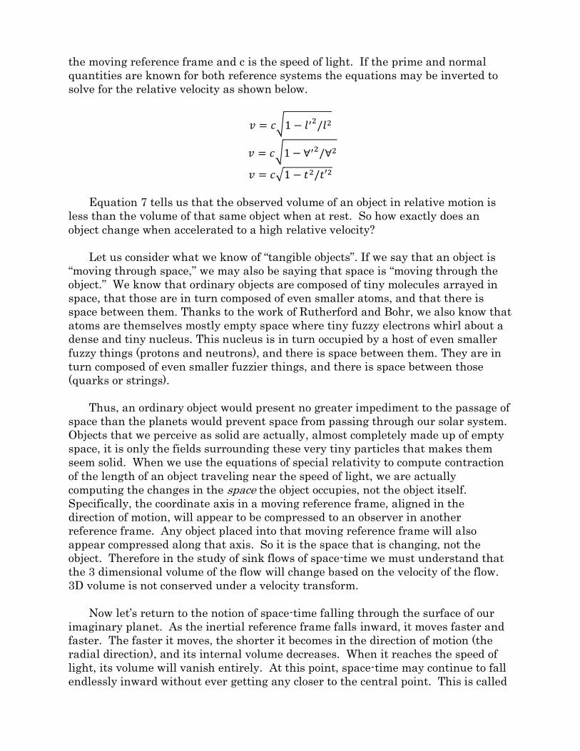
object or a black hole. Figure 6-1 shows how a FST black hole is conceptually
different from a black hole for mainstream physics.
Figure 6-1
Both black holes have a funnel shape and transition from essentially flat space
into a region of highly curved space. Both describe a gravitational field. Both have
an event horizon which divides normal space from complex space (more about that
later). Going beyond the event horizon, the traditional black hole has a region of
superluminal velocity that continues down to a singularity. Beyond the event
horizon of the FST black hole, the velocity may or may not be superluminal and
there is no more tapering down, instead there is a space-time discontinuity of finite
size.
Another profound difference between a FST black hole and the traditional black
hole is that while everything the makes up the traditional black hole is
concentrated far below the event horizon in a singularity, everything that makes up
the FST black hole (energy, matter, momentum, entropy, etc) lies above the event
horizon. Inside the event horizon of the FST black hole lies a domain that is not
part of our universe. Our space-time coordinates don’t go there. It is a bubble of
something else, a discontinuity. If anything lies inside, what it is cannot be known.
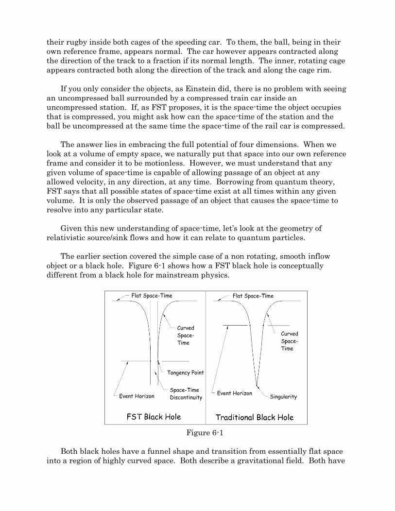
As presently define a FST black hole can be made from any amount of energy
and have a rmin of any size. It is also smooth round and not rotating. If the inflow
of space-time is not smooth, a number of possible vibrations could take place.
Rather than level out at velocity c, irregularities in the flow may cause the core of
the flow stream to become superluminal.
As sown in Figure 3-2, the acceleration curve at rmin (flow velocity =c)
acceleration is zero, meaning that gravity has stopped and there is no more
accelerating force. There is nothing to drive further acceleration above c or cause
any further reduction in the size of the flow stream below rmin. If the curve is
continued beyond rmin, the acceleration becomes negative, which would result in
push back against the flow.
Figure 6-2

In superluminal flow, below rmin, the term under the radical in the velocity
equation becomes negative and the solution becomes a combination of real and
imaginary numbers, a complex number. Following the curve in figure 3-2, when the
velocity becomes superluminal acceleration becomes negative, creating a repulsive
force to drive the velocity back below c. At this point the flow stream may oscillate
between sub and superluminal velocity, or between real and complex space-time.
From the point of view inside the flow field at the event horizon, two spatial
dimensions (up/down and left/right) are restricted to very tiny values. The
inward/outward dimension, however, is infinite. From the point of view outside the
flow field, time at the event horizon has come to a virtual stop. In this way, a four
dimensional flow field transitions into an essentially one dimensional object. This
one dimensional object will be very stiff and could behave like a piano string. See
figure 6-2 for possible vibration modes of a FST object. Thus, at the heart of a fluid
space inflow field, there is found a complex harmonic oscillator. This oscillation
would best be described by a wave function involving complex numbers.
We may now proceed to develop quantum and string theory in harmonious
connection with a gravitational object.

Section 7: Gravity and Electromagnetism.
Another well known parallel between gravity and electromagnetism is
Coulombs law for static charges.
Which has an identical form to Newton’s equation for gravity.
I believe this is no coincidence and potentially enlightening. In Coulomb’s
equation ke plays the role of G and charge plays the role of mass. The SI units for ke
are kilogram meters cubed per second squared Coulombs squared. Whereas G has
units of meters cubed per kilogram second squared. Both constants have a time
change of spatial flux term, m3/s2. This suggests that charge may also be a
manifestation of an energized spatial flow.
If the time change of spatial flux term is removed we are left with kg/C2 from
ke and 1/kg from G. If there were a mass energy equivalent for charge like E=qc2 or
an energy conversion factor between coulombs and kilograms, ke would reduce to
the exact same units as G. Let’s look for that conversion factor. Assume that the
matter energy equivalence may be related to a similar charge energy equivalence
through a conversion factor H.
First we find a set of charges and masses such that:
Dividing out the r’s and substituting H for m1/q1 and m2/q2 we get.
Punching in the numbers yields.
This tells us that it would take 1.16 times 1010 kilograms of matter to create the
same gravitational force as the electric force produced by 1 coulomb of charge. This
can’t be the first time in human history that this number has been calculated. If
the energy equivalence equation holds, then there is far more energy tied up in the

form of charge in the universe than there is in matter. This energy, if present, does
not create gravity nor show itself in terms of mass and momentum in the material
elements it is attached to and only acts on other elements of charge. This all seems
very unlikely. While the value of H is probably valid in the comparison of forces, it
may not be useful in terms of calculating energy content. It is more likely that
electromagnetism has a different space-time flow pattern involving another
dimensional axis, replacing the x, y, z, or tc with a new axis perpendicular to the
one it replaces. The spacetial distortion energy associated with the new axis could
be quite different from that of the tc axis. Since we see charge acting in x, y, and z,
it must be the tc axis that has been replaced. This would also prevent electric
charge from interacting with time and gravity.
It may be helpful to think of a gravitational field as a four dimensional object in
rotation about a plane or pair of planes. Visualization of such an object is difficult,
however a 4D hyper-sphere rotating about the z-y and x-tc planes could appear in
3D space as an inflow/outflow field. Another pairing of planes might account for
electromagnetic fields.
It is important keep in mind that these objects are fluid, not made of elastic
membranes or solids. As fluid forms, they will take the shape necessary to keep all
forces in balance and be flexible and self-correcting when acted upon by an outside
force. This may be viewed similarly to the way charge distribution inside a
conductor flows to always keep the electric potential equal to zero.
Figure 7-1
Figure 7-1 shows a 3Sphere intersecting a plane. If the surface of this sphere is
projected onto the plane and the sphere is rotating at a constant rate about the
vertical axis, a two dimensional being living on the plane will see a circle in which
area magically appears on one side of the circle, travels across the circle and
vanishes on the other side.

Figure 7-2
The left image of Figure 7-2 shows a bounding volume of a 4Sphere around the
time axis. The right image is a close-up of the center, showing that the passage
does not go to zero but has a minimum radius Rmin. The surfaces in these images
represent volumes in which the dimension normal to the surface has been
compressed to zero and the green axis in the figure is the time axis. Imagine that
the torus is rolling along the time axis like a smoke ring. If the surface (volume) of
the torus is projected onto the central plane (volume), a 3D being living in that
volume will see space magically appear at the edge and accelerate toward the center
where it will slow and then vanish at Rmin. This is exactly what we see in the
gravity field of a material object. A FST inflow field can be viewed as an energized
hyper-sphere rolling along the time axis.
Only one bounding volume is shown in Figure 16 but there would be an infinite
number of them ranging in size from Rmin to infinity, all rolling along the time axis,
each representing a radius/velocity profile proportional to the central mass. This
rolling smoke ring form is shared by all material objects and is nested in space-time
with all other objects as in a fractal pattern encompassing the entire universe.
In a doughnut shaped universe (like the one in Figure 7-2 or like the one stolen
from Homer Simpson by Stephen Hawking), The “Big Bang” would not be an event
but a permanent feature of the universe where recycled energy is spewed out
continuously on one side, travels around the torus and is eventually swallowed up
on the other end only to be spewed out once more (no need for inflation).
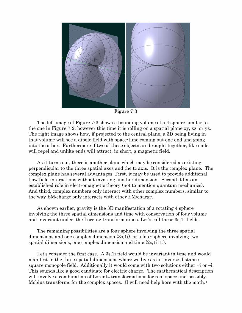
Figure 7-3
The left image of Figure 7-3 shows a bounding volume of a 4 sphere similar to
the one in Figure 7-2, however this time it is rolling on a spatial plane xy, xz, or yz.
The right image shows how, if projected to the central plane, a 3D being living in
that volume will see a dipole field with space-time coming out one end and going
into the other. Furthermore if two of these objects are brought together, like ends
will repel and unlike ends will attract, in short, a magnetic field.
As it turns out, there is another plane which may be considered as existing
perpendicular to the three spatial axes and the tc axis. It is the complex plane. The
complex plane has several advantages. First, it may be used to provide additional
flow field interactions without invoking another dimension. Second it has an
established role in electromagnetic theory (not to mention quantum mechanics).
And third, complex numbers only interact with other complex numbers, similar to
the way EM/charge only interacts with other EM/charge.
As shown earlier, gravity is the 3D manifestation of a rotating 4 sphere
involving the three spatial dimensions and time with conservation of four volume
and invariant under the Lorentz transformations. Let’s call these 3s,1t fields.
The remaining possibilities are a four sphere involving the three spatial
dimensions and one complex dimension (3s,1i), or a four sphere involving two
spatial dimensions, one complex dimension and time (2s,1i,1t).
Let’s consider the first case. A 3s,1i field would be invariant in time and would
manifest in the three spatial dimensions where we live as an inverse distance
square monopole field. Additionally it would come with two solutions either +i or –i.
This sounds like a good candidate for electric charge. The mathematical description
will involve a combination of Lorentz transformations for real space and possibly
Mobius transforms for the complex spaces. (I will need help here with the math.)

The second case (2s,1i,1t) will be a time dependant field which would manifest
in 3D real space as a dipole field with the solutions for +i and –i simply flipping the
polarity. This is a good candidate for magnetism. (once again, I will need help with
the math.)
These fields will be limited in how they can attach, or stem from the 3s,1t
spatial inflow fields described in the earlier sections. These attachments or
stemmings can only happen at the heart of the inflow at the critical energy levels
where the flow field oscillates between real and complex space.
Let’s take a look at 3s,1i space and apply the same reasoning we used for
Minkowski space (3s,1t). While three dimensional volume is not conserved in
spatial flows, four dimensional volume is conserved. Four volume is defined as
follows for 3s,1i space.
Under a Lorentz transformation four volume is unchanged (x1=x1’ and x2=x2’).
The terms under the radical are still expressed in terms of gravitational fields.
Let’s see if they can be expressed in terms of electromagnetism. We will make the
following substitutions.
Thus
And now we have:
We can now retrace all the reasoning applied so far to gravitational flow fields
on these complex flow fields. In this case rather than looking at how the spatial
dimensions change with time, we look at how they change with respect to the
complex dimension X4. We will arrive at a pair of monopole, inverse distance

square fields, with opposite signs. These will manifest in space-time whenever they
become attached to a space-time flow field as described earlier, sharing the spatial
dimensions but invariant or immune to the effects of time. In particle physics,
charge is always found in conjunction with a particle that has the property of mass.
But some particles that have mass do not carry charge. For this reason I present
the following. I postulate that 3s,1i fields can only exist when attached to a 3s,1t
field but a 3s,1t field can exist without a 3s,1i field (or with two opposite
superimposed 3s,1i fields). This is the basis of electric charge and how it is linked
to gravity. All of current EM theory descends directly without change but with a
new basis founded on spatial flow fields.
My primary question at this point is if and how these complex 3s,1i flow fields
may be used to influence 3s,1t flow fields.
This is as far as I have written. I have further speculations but development is
incomplete.
Copyright 2017, John S. Huenefeld. All rights reserved.