Embed Size (px)
Citation preview

Fluids
University of Oxford
Third Year, Part B1
Caroline Terquem
Department of Physics
Hilary Term 2021

2
Contents
1 Kinematics of fluids 5
1.1 What is a fluid? . . . . . . . . . . . . . . . . . . . . . . . . . . . . . . . . . . 5
1.1.1 Mean free path . . . . . . . . . . . . . . . . . . . . . . . . . . . . . . 6
1.1.2 Averaged quantities . . . . . . . . . . . . . . . . . . . . . . . . . . . 6
1.2 Eulerian and Lagrangian descriptions . . . . . . . . . . . . . . . . . . . . . . 7
1.3 Streamlines, trajectories and streamtubes . . . . . . . . . . . . . . . . . . . 8
1.4 Material time derivative . . . . . . . . . . . . . . . . . . . . . . . . . . . . . 8
1.4.1 Acceleration of a fluid element: . . . . . . . . . . . . . . . . . . . . . 10
1.4.2 Steady flow . . . . . . . . . . . . . . . . . . . . . . . . . . . . . . . . 11
1.4.3 Rate of change along a streamline . . . . . . . . . . . . . . . . . . . 11
1.5 Vorticity and strain rate . . . . . . . . . . . . . . . . . . . . . . . . . . . . . 12
1.5.1 Rate of strain tensor . . . . . . . . . . . . . . . . . . . . . . . . . . . 13
1.5.2 Vorticity . . . . . . . . . . . . . . . . . . . . . . . . . . . . . . . . . . 15
1.5.3 Deformation of a fluid element in the general case . . . . . . . . . . 16
1.6 Mass conservation . . . . . . . . . . . . . . . . . . . . . . . . . . . . . . . . 17
1.6.1 Eulerian approach . . . . . . . . . . . . . . . . . . . . . . . . . . . . 17
1.6.2 Lagrangian approach . . . . . . . . . . . . . . . . . . . . . . . . . . . 18
1.7 Incompressibility . . . . . . . . . . . . . . . . . . . . . . . . . . . . . . . . . 18
1.8 Velocity potential, circulation and stream function . . . . . . . . . . . . . . 19
1.8.1 Velocity potential . . . . . . . . . . . . . . . . . . . . . . . . . . . . . 19
1.8.2 Circulation . . . . . . . . . . . . . . . . . . . . . . . . . . . . . . . . 20
1.8.3 Stream function . . . . . . . . . . . . . . . . . . . . . . . . . . . . . 22
2 Dynamics of fluids 23
2.1 Stress tensor . . . . . . . . . . . . . . . . . . . . . . . . . . . . . . . . . . . 23
2.1.1 Pressure and viscous forces in fluids . . . . . . . . . . . . . . . . . . 24
2.1.2 Definition of the stress tensor . . . . . . . . . . . . . . . . . . . . . . 25
2.1.3 Two–dimensional shear flow in a gas . . . . . . . . . . . . . . . . . . 26
2.1.4 Stress tensor and velocity correlations . . . . . . . . . . . . . . . . . 28
2.1.5 Expression of the stress tensor for a Newtonian fluid . . . . . . . . . 29
2.2 Equation of motion for a fluid . . . . . . . . . . . . . . . . . . . . . . . . . . 32
2.2.1 Navier–Stokes equation . . . . . . . . . . . . . . . . . . . . . . . . . 32
2.2.2 Reynolds number . . . . . . . . . . . . . . . . . . . . . . . . . . . . . 35
3

2.2.3 Dimensional analysis and similarity . . . . . . . . . . . . . . . . . . . 36
2.2.4 Incompressibility revisited . . . . . . . . . . . . . . . . . . . . . . . . 38
2.2.5 Euler equation for an inviscid fluid . . . . . . . . . . . . . . . . . . . 39
2.3 Boundary conditions . . . . . . . . . . . . . . . . . . . . . . . . . . . . . . . 39
2.3.1 Rigid boundary . . . . . . . . . . . . . . . . . . . . . . . . . . . . . . 39
2.3.2 Interface between two fluids . . . . . . . . . . . . . . . . . . . . . . . 41
2.3.3 Free surface . . . . . . . . . . . . . . . . . . . . . . . . . . . . . . . . 44
2.4 The vorticity equation and Kelvin’s theorem . . . . . . . . . . . . . . . . . . 44
2.4.1 The vorticity equation for an incompressible viscous fluid . . . . . . 45
2.4.2 Case of an ideal fluid and Kelvin’s theorem . . . . . . . . . . . . . . 46
2.5 Conservation of energy and Bernoulli’s theorem . . . . . . . . . . . . . . . . 48
2.5.1 Conservation of energy in an incompressible Newtonian fluid . . . . 48
2.5.2 Conservation of energy in a steady ideal fluid: Bernoulli’s theorem . 51
2.6 Examples of viscous flows and very viscous flows . . . . . . . . . . . . . . . 52
3 Potential flows 53
3.1 General properties of potential flows . . . . . . . . . . . . . . . . . . . . . . 54
3.2 Simple potential flows . . . . . . . . . . . . . . . . . . . . . . . . . . . . . . 55
3.2.1 Uniform parallel flows . . . . . . . . . . . . . . . . . . . . . . . . . . 55
3.2.2 Line vortex flow . . . . . . . . . . . . . . . . . . . . . . . . . . . . . 56
3.2.3 Sources and sinks . . . . . . . . . . . . . . . . . . . . . . . . . . . . . 57
3.2.4 Dipole flow . . . . . . . . . . . . . . . . . . . . . . . . . . . . . . . . 57
3.2.5 Flow around a circular cylinder . . . . . . . . . . . . . . . . . . . . . 58
3.3 Complex velocity potential . . . . . . . . . . . . . . . . . . . . . . . . . . . 63
3.3.1 Cauchy–Riemann equations . . . . . . . . . . . . . . . . . . . . . . . 63
3.3.2 Complex potential of a flow past a cylinder . . . . . . . . . . . . . . 64
3.3.3 Conformal mapping . . . . . . . . . . . . . . . . . . . . . . . . . . . 64
3.3.4 The Joukowski transformation . . . . . . . . . . . . . . . . . . . . . 67
3.3.5 Potential flow past a finite plate and the Kutta condition . . . . . . 68
3.3.6 The Joukowski aerofoil . . . . . . . . . . . . . . . . . . . . . . . . . . 70
3.3.7 Forces on aerofoils and the Kutta–Joukowski theorem . . . . . . . . 71
3.3.8 The origin of the circulation . . . . . . . . . . . . . . . . . . . . . . . 74
4 Boundary layers 77
4.1 The boundary layer on a flat plate . . . . . . . . . . . . . . . . . . . . . . . 78
4.1.1 Thickness of the boundary layer . . . . . . . . . . . . . . . . . . . . 78
4.1.2 Equation of motion . . . . . . . . . . . . . . . . . . . . . . . . . . . . 79
4.1.3 Velocity profile in the boundary layer . . . . . . . . . . . . . . . . . 80
4.1.4 Frictional force on a flat plate . . . . . . . . . . . . . . . . . . . . . . 82
4.1.5 Vorticity in the boundary layer and wake . . . . . . . . . . . . . . . 83
4.1.6 Transition to turbulence . . . . . . . . . . . . . . . . . . . . . . . . . 83
4.2 Boundary layer separation . . . . . . . . . . . . . . . . . . . . . . . . . . . . 85
4

4.2.1 Condition for separation . . . . . . . . . . . . . . . . . . . . . . . . . 85
4.2.2 Effect of the Reynolds number on the separation . . . . . . . . . . . 87
4.2.3 Enhanced drag . . . . . . . . . . . . . . . . . . . . . . . . . . . . . . 88
5 Waves 91
5.1 Sound waves . . . . . . . . . . . . . . . . . . . . . . . . . . . . . . . . . . . 91
5.1.1 Wave equation in a perfect gas . . . . . . . . . . . . . . . . . . . . . 92
5.1.2 Wave equation in a liquid . . . . . . . . . . . . . . . . . . . . . . . . 93
5.1.3 The speed of sound . . . . . . . . . . . . . . . . . . . . . . . . . . . . 94
5.1.4 Solutions to the wave equation . . . . . . . . . . . . . . . . . . . . . 95
5.1.5 Energy in sound waves . . . . . . . . . . . . . . . . . . . . . . . . . . 95
5.2 Surface waves . . . . . . . . . . . . . . . . . . . . . . . . . . . . . . . . . . . 95
5.2.1 Equilibrium state . . . . . . . . . . . . . . . . . . . . . . . . . . . . . 96
5.2.2 Boundary conditions . . . . . . . . . . . . . . . . . . . . . . . . . . . 96
5.2.3 Equation and boundary conditions for the velocity potential . . . . . 98
5.2.4 Dispersion relation . . . . . . . . . . . . . . . . . . . . . . . . . . . . 99
5.2.5 Dispersion and group velocity . . . . . . . . . . . . . . . . . . . . . . 101
5.2.6 Surface gravity waves on deep water . . . . . . . . . . . . . . . . . . 102
5.2.7 Surface gravity waves on water of finite depth . . . . . . . . . . . . . 104
5.2.8 Gravity–capillary waves . . . . . . . . . . . . . . . . . . . . . . . . . 105
5.3 Internal gravity waves . . . . . . . . . . . . . . . . . . . . . . . . . . . . . . 106
5.3.1 Buoyancy frequency . . . . . . . . . . . . . . . . . . . . . . . . . . . 106
5.3.2 Dispersion relation . . . . . . . . . . . . . . . . . . . . . . . . . . . . 107
5.3.3 Motion of fluid elements . . . . . . . . . . . . . . . . . . . . . . . . . 109
6 Instabilities and turbulence 111
6.1 Kelvin–Helmholtz instability . . . . . . . . . . . . . . . . . . . . . . . . . . 111
6.1.1 Boundary conditions . . . . . . . . . . . . . . . . . . . . . . . . . . . 112
6.1.2 Dispersion relation . . . . . . . . . . . . . . . . . . . . . . . . . . . . 112
6.1.3 Instability condition . . . . . . . . . . . . . . . . . . . . . . . . . . . 114
6.1.4 Physics of the instability . . . . . . . . . . . . . . . . . . . . . . . . . 115
6.2 Rayleigh–Taylor instability . . . . . . . . . . . . . . . . . . . . . . . . . . . 116
6.3 Turbulence . . . . . . . . . . . . . . . . . . . . . . . . . . . . . . . . . . . . 117
6.3.1 The Reynolds stress . . . . . . . . . . . . . . . . . . . . . . . . . . . 117
6.3.2 Mixing length theory . . . . . . . . . . . . . . . . . . . . . . . . . . . 119
6.3.3 Energy conservation . . . . . . . . . . . . . . . . . . . . . . . . . . . 119
6.3.4 Kolmogorov scaling . . . . . . . . . . . . . . . . . . . . . . . . . . . 121
A Complex variables 123
A.1 The Cauchy–Riemann relations . . . . . . . . . . . . . . . . . . . . . . . . . 123
A.2 Cauchy’s theorem . . . . . . . . . . . . . . . . . . . . . . . . . . . . . . . . . 124
A.3 Laurent series . . . . . . . . . . . . . . . . . . . . . . . . . . . . . . . . . . . 124
5

Fluid dynamicists were divided into hydraulic engineers who observe what cannot be ex-
plained and mathematicians who explain things that cannot be observed.
Sir Cyril Hinshelwood (in Lighthill, 1956)
These notes borrow from the following books:
E. Guyon, J.–P. Hulin, L. Petit, C. D. Mitescu, Physical Hydrodynamics, 2nd edition
(Oxford University Press)
D. J. Acheson, Elementary Fluid Dynamics (Oxford University Press)
L. D. Landau, E. M. Lifshitz, Fluid Mechanics, 2nd edition, Volume 6 of Course of
Theoretical Physics (Elsevier)
G. K. Batchelor, An introduction to Fluid Dynamics (Cambridge University Press)
These notes are meant to be a support for the course, but they should not replace text-
books. It is strongly advised that at least one of the books listed above is used regularly,
as they provide much more details about the subject and lots of examples and problems.
6

Chapter 1
Kinematics of fluids
1.1 What is a fluid?
A fluid is a collection of particles that can be treated as a continuum and which flows
(deforms) when acted upon by a stress.
When particles are free to move relative to each other, the description as a continuum
requires their mean free path to be much smaller than the other characteristic lengths of
the problem. This condition is usually met in liquids and may also be satisfied in gases
and plasmas. Solids, in which particles are bound to their neighbours, can be described as
a continuum on scales large compared to inter–atomic distances (e.g., theory of elasticity).
In cases where the continuum approximation does not apply, kinetic theory has to be used.
Hydrodynamics can actually be obtained as the limit of kinetic theory when the mean free
path is much smaller than all the other characteristic lengths.
Liquids, gases and plasmas all deform under stress and therefore may be treated as fluids.
In general, solids are not considered as fluids because they do not deform easily. However,
some solids do flow when subject to stresses larger than their limit of elasticity. Examples
of this are glaciers and the Earth’s crust. Also, some materials behave either like solids or
liquids depending on whether they are subject to a high or low frequency stress, respec-
tively. For instance, we sink deeper into wet sand when standing up than when running.
Also some polymers, which behave like solids when acted upon by a stress that varies on
a short timescale, start to behave like liquids when the stress varies on a timescale long
enough that the polymer can use its internal degrees of freedom to deform like a liquid.
The frontier between solids and liquids can therefore be fuzzy.
7

1.1.1 Mean free path
The mean free path λ is the average distance travelled by a particule before it collides
with another particle. It is given by:
λ ∼ 1
nσ, (1.1)
where n is the number density of particles and σ is the collision cross section. If all the
particles are identical and with diameter d, then σ = πd2.
Let us calculate the mean free path of the molecules in air at atmospheric pressure
and room temperature. Air consists of 21% of O2 and 78% of N2 (and small amounts of
other gases), which have a diameter d ' 0.4 nm. Treating the air as an ideal gas, the
number density is given by n = P/(kT ), where P is the pressure, T is the temperature
and k is the Boltzmann constant. Adopting P = 1 atm = 1.01× 10⁵ Pa and T = 300 K,
we obtain n = 2.4 × 1025 m−3. The collision cross section is σ = πd2 = 5 × 10⁻¹⁹ m2.
Therefore λ ' 8× 10⁻⁸ m, which indicates that the fluid approximation applies unless we
are interested in microscopic processes.
1.1.2 Averaged quantities
If the mean free path λ is very much smaller than the scale of interest L in the system,
we can characterize a volume element with scale l such that λ l L using averaged
quantities. For example, the velocity of a single particle can be written as u = v + w,
where v is the same average velocity for all the particles in the volume (since l L), and
w is a fluctuating part. In a volume element with l λ, particles suffer a large number of
collisions so that w changes sign very rapidly. Therefore, as illustrated in the figure below,
the displacement of the particles in this volume over an interval of time ∆t is given by
v∆t, as w averages to zero, and the volume element is always made of the same particles
as it moves.
For most purposes, we can therefore neglect w and define u = v as being the velocity of
the fluid element. In the same way, the temperature, pressure, etc., can be defined as an
average over the large number of particules in the volume. Thereafter, fluid elements will
be sometimes loosely referred to as particles.
8

1.2 Eulerian and Lagrangian descriptions
A flow can be described in two different ways, depending on how the variations of the
different quantities (velocity, density, temperature, etc.) are considered:
• In the Eulerian description, the variations are described as a function of time at
all fixed points in the flow. The velocity v(r, t) of a fluid element which at time t
coincides with the fixed point located at r is that seen by the fox at rest on the river
bank. In this description, the velocity is a vector field. Such a velocity field would
be measured by fixed probes embedded in the fluid.
• In the Lagrangian description, one follows individual fluid elements moving with
the flow and variations are described as a function of time. The velocity V(t, r0)
of a fluid element which at some time t0 is at position r0 is that of the duck in
the river. (We denote the Lagrangian velocity with a capital letter to distinguish it
from the Eulerian velocity). The parameter r0 simply ’tags’ the path along which
the fluid element is moving. Such a velocity can be measured by tracking (e.g.,
phosphorescent) tracer particles. If at a time t′ the duck is a the position r′, then its
Lagrangian velocity at that time coincides with the Eulerian velocity at that point
and time: V(t′, r0) = v(r′, t′).
9

1.3 Streamlines, trajectories and streamtubes
A streamline is, at any particular time t, a curve whose tangent is everywhere parallel to
the velocity vector. Let us consider a point (x, y, z) on a streamline. A small displacement
(dx,dy,dz) along the streamline is then parallel to v(x, y, z), which implies that:
dx
vx=
dy
vy=
dz
vz. (1.2)
Integrating these two differential equations yields the equation of the streamlines.
Streamlines at a given time do not
intersect, because a particle at a
given point cannot have two different
velocities at the same time.
A trajectory (or pathline) is the path
followed by a particle. Trajectories
can intersect.
Streamlines and trajectories only coincide in a steady flow. This can be seen by noting
that M1 which, at t0, is on the streamline which is represented above, will have advanced
to M2 at a subsequent time t1 only if the velocity does not change between t0 and t1.
A streamtube is a set of streamlines
that are drawn through each point of
a closed curve.
1.4 Material time derivative
We consider a Eulerian quantity Q (e.g., temperature, density, etc.), that is to say a
quantity which is specified at a fixed position at a given time. For a fluid element which
at time t is at a point located at r, the value of this quantity is Q(r, t). If the Eulerian
velocity at this point is v(r, t), then at time t + δt the fluid element is at r + vδt, where
10

the value of Q is Q(r + vδt, t + δt). The time rate of change of Q for this fluid element,
which we denote by DQ/Dt, is therefore:
DQ
Dt= lim
δt→0
Q(r + vδt, t+ δt)−Q(r, t)
δt. (1.3)
Performing a Taylor series expansion to first order in δt:
Q(r + vδt, t+ δt) = Q(r, t) + δt∂Q(r, t)
∂t+ vδt ·∇Q(r, t), (1.4)
equation (1.3) becomes:
DQ
Dt=∂Q
∂t+ v ·∇Q. (1.5)
The time derivative following the motion of a fluid element is then given by the following
operator:
D
Dt=
∂
∂t+ v ·∇ , (1.6)
which is also called material time derivative or Lagrangian rate of change. The way it
has been calculated here, it has meaning only when applied to a Eulerian quantity which
depends on the two independent variables r and t. However, this is not a unique approach1.
From equation (1.6), we see that there are two contributions to DQ/Dt: ∂Q/∂t, which
is the local rate of change due to time variations of Q at a fixed point, and v ·∇Q, which
is due to the fluid element being transported to a different position along the gradient of
Q (see below). The first term is the Eulerian rate of change, whereas the second term is
the convective rate of change.
If Q is a constant for every fluid element, then DQ/Dt = 0. It does not mean though
that it is a constant through the fluid, as it may be a different constant for different fluid
elements. It only means that a fluid element having a given value of Q at some particular
time will retain this value of Q at any subsequent time.
1Mathematically, the operator D/Dt could also be defined as the total time derivative of a function
which depends both on r(t) and on t explicitely. Indeed, the quantity Q could be seen as depending
explicitely on time, and also on the location r, which itself depends on time: Q(r(t), t). The rate of change
of Q is then just its total time derivative:
dQ(r(t), t)
dt=∂Q
∂t+∂Q
∂x
dx
dt+∂Q
∂y
dy
dt+∂Q
∂z
dz
dt.
Using vx = dx/dt, vy = dy/dt and vz = dz/dt, we obtain:
dQ(r(t), t)
dt=∂Q
∂t+ v ·∇Q,
which is the same as DQ/Dt. However, note that Q(r(t), t) is neither the Eulerian representation of Q, as
this is given by Q(r, t) where r is fixed, nor the Lagrangian representation, as this is given by Q(r0, t) and
is independent of r.
11

1.4.1 Acceleration of a fluid element:
Above, we have calculated the material time derivative of a scalar Q, but the operator
D/Dt could also be applied to a vector. For example, to calculate the acceleration of
a fluid element, or Lagrangian acceleration, we have to calculate Dv/Dt. Applying the
operator to each of the cartesian coordinates of the velocity, it is straightforward to see
that:
Dv
Dt=∂v
∂t+ (v ·∇) v , (1.7)
where the operator is applied to the Eulerian velocity v(r, t). Note that ∂v/∂t is not the
acceleration of a fluid element at location r at time t, because the element is there only
instantaneously.
In cartesian coordinates, the components of (v ·∇) v are given by:
vx∂vx∂x
+ vy∂vx∂y
+ vz∂vx∂z
,
vx∂vy∂x
+ vy∂vy∂y
+ vz∂vy∂z
,
vx∂vz∂x
+ vy∂vz∂y
+ vz∂vz∂z
.
To use the above formula in other coordinate systems, we have to take into account the
fact that the unit vectors depend on the space coordinates. For example, in cylindrical
coordinates (r, θ, z):
(v ·∇) v =
(vr∂
∂r+ vθ
∂
r∂θ+ vz
∂
∂z
)(vrr + vθθ + vzz
),
where r, θ and z denote the unit vectors. Remembering that ∂θ/∂θ = −r, we see that,
for example, the radial component of this expression has a term −v2θ/r that comes from
∂(vθθ)/∂θ.
The acceleration of a fluid element could also be calculated directly using the La-
grangian representation of the velocity V(r0, t). In this case, it is just the time derivative
of the velocity along a given path, so that:
Dv
Dt=
(∂V
∂t
)r0
. (1.8)
Note that the velocity of a fluid element can be written as:
v =Dr
Dt. (1.9)
12

This can be seen by writing that the operator applies to the Eulerian quantity r = xx +
yy + zz, where a hat denotes a unit vector, so that there is no time dependence and:
Dr
Dt= (v ·∇) r = vx
dx
dxx + vy
dy
dyy + vz
dz
dzz = v.
1.4.2 Steady flow
It is a flow in which, at any fixed point r, the velocity does not depend on time, that is to
say:
∂v
∂t= 0. (1.10)
We see from equation (1.7) that, in a steady flow, fluid elements may still be accelerated
by being transported to a position where the velocity has a different value.
Consider for example a fluid in uniform rotation with angular velocity Ω, so that
vx = −Ωy, vy = Ωx and vz = 0. Then:
(v ·∇) v =
(−Ωy
∂
∂x+ Ωx
∂
∂y
)(−Ωy,Ωx, 0) = −Ω2(x, y, 0),
which is, as expected, the centripetal acceleration −Ω2r.
1.4.3 Rate of change along a streamline
In a steady flow, the Lagrangian rate of change of a quantity Q is given by v ·∇Q. Let
us denote s the coordinate (distance) along a streamline, and s the unit vector associated
with this coordinate. Then v = |v|s and
v ·∇Q = |v|s ·∇Q = |v|∂Q∂s
. (1.11)
This is the rate of change of Q with distance along the streamline times the flow speed,
which gives the rate of change of Q with time along the streamline.
Therefore, v ·∇Q = 0 means that Q is constant along a streamline, that is to say for
a fluid element moving along that streamline.
13

1.5 Vorticity and strain rate
Here we are interested in the way a small volume of fluid deforms when it moves with the
flow. In the figure below, the velocity is not uniform across the volume, so that it tilts and
stretches as it moves:
At time t, the velocity of a particle at location r is v(r, t) and that of a particle at
location r+ dr is v + dv. To first order in the components dxj (j = 1, 2, 3) of dr, we have:
dvi =∂vi∂xj
dxj . (1.12)
Einstein notation2 has been used in this equation and will be used throughout these notes.
We use either (x1, x2, x3) or (x, y, z) to denote the x–, y– and z–components.
The quantity Dij ≡ ∂vi/∂xj is called the deformation tensor. If we select a corner of
the cube on the figure above as a reference point, then Dij tells us how the points in the
cube move with respect to this reference point. Therefore, it contains information about
how the cube deforms as it moves, but does not describe the overall motion of the cube
with the flow. This tensor can be written as Dij = eij + ωij , where eij is a symmetric
tensor and ωij is an anti-symmetric tensor which are given by:
eij =1
2
(∂vi∂xj
+∂vj∂xi
), rate of strain tensor (1.13)
ωij =1
2
(∂vi∂xj− ∂vj∂xi
), vorticity tensor. (1.14)
The strain is a measure of the local deformation of a fluid element caused by an applied
stress, whereas the vorticity measures the local angular velocity of the fluid element, as
will be made clear below.
2Einstein notation implies that repeated indices within one term are summed over. Therefore,
∂vi∂xj
dxj ≡3∑j=1
∂vi∂xj
dxj .
14

1.5.1 Rate of strain tensor
We are going to show that the diagonal terms of the tensor eij are associated with a change
in volume whereas off-diagonal terms are associated with shear.
Diagonal terms:
We assume here that only the diagonal terms, of the form ∂vi/∂xi, are non–zero.
Let us consider the volume element repre-
sented in the figure at time t. Its volume is
V (t) = ∆x1∆x2∆x3. We are now going to
calculate its volume V (t+ δt) at time t+ δt.
We note v(x1, x2, x3, t) the velocity at point (x1, x2, x3) and at time t. To first order in
δt, point A moves away from O at the relative velocity:
vrel = v(∆x1, 0, 0, t)− v(0, 0, 0, t) = ∆x1∂v1
∂x1x1,
where x1 is the unit vector in the x1–direction and the velocity in the derivative is evaluated
at O and at time t. The distance traveled by point A relative to O between t and t+ δt is
|vrel|δt and the distance OA(t+ δt) between O and A at t+ δt is obtained by adding ∆x1:
OA(t+ δt) = ∆x1 + ∆x1∂v1
∂x1δt.
We have assumed here that the displacement of a point which is initially at ∆x1 is
v(∆x1)δt, that is to say we have not taken into account the variations of v between t
and t + δt. This is only valid to first order in δt when the deformations are very small.
This calculation could have been done for any point belonging to the x = ∆x1 plane, which
means that this face of the cuboid is moving along the x1–axis while staying parallel to
its original direction. Similarly, along the x2– and x3–directions:
OB(t+ δt) = ∆x2 + ∆x2∂v2
∂x2δt,
OC(t+ δt) = ∆x3 + ∆x3∂v3
∂x3δt,
and, again, the faces of the cuboid in the y = ∆x2 and z = ∆x3 planes move while staying
parallel to their original direction.
15

Therefore, there is no tilting but only stretching:
the cuboid only dilates or contracts.
The volume at t+ δt is:
V (t+ δt) = ∆x1∆x2∆x3
(1 +
∂v1
∂x1δt
)(1 +
∂v2
∂x2δt
)(1 +
∂v3
∂x3δt
),
which, to first order in δt, is equal to:
V (t+ δt) = ∆x1∆x2∆x3
[1 + δt
(∂v1
∂x1+∂v2
∂x2+∂v3
∂x3
)].
This can be written as:
V (t+ δt) = V (t) (1 + δt∇ · v) .
If we note δV the change in volume during δt, then the relative change in volume is:
δV
V= δt∇ · v, (1.15)
which expresses the fact that the rate of volume expansion is ∇ · v, which is also equal to
eii, the trace of the tensor eij .
Off–diagonal terms:
We now assume that only the off–diagonal terms, of the form ∂vi/∂xj with j 6= i, are non–
zero. We limit the discussion to the two dimensional case to keep the analysis simpler,
noting that it can easily be extended to three dimensions.
We consider the surface element OADB
represented in the figure at time t. Since v1
depends only on x2, A moves relative to O
in the x2–direction. Similarly, B moves rel-
ative to O in the x1–direction. The dashed
lines represent the surface at time t+δt (here
and thereafter we ignore the translation of
the whole surface).
16

To first order in δt, point A moves relative to O at the velocity:
vrel = v(∆x1, 0, 0, t)− v(0, 0, 0, t) = ∆x1∂v2
∂x1x2,
where x2 is the unit vector in the x2–direction and the velocity in the derivative is eval-
uated at O and at time t. Therefore, after a time δt, OA becomes OA′ with AA′ =
∆x1(∂v2/∂x1)δt. The angle δα through which the line rotates during δt is then given by
δα ' AA′/OA = (∂v2/∂x1)δt (positive angles are defined counterclockwise). Similarly,
OB rotates through δβ ' −(∂v1/∂x2)δt (this angle is negative if, as assumed in the figure,
∂v1/∂x2 > 0.) If δα = δβ, the angle γ between the lines OA and OB remains constant:
there is only rotation. However, when δα 6= δβ, γ changes by δγ = δβ − δα (which on the
figure is negative): there is shearing motion. The angle δγ is called the shear strain of the
fluid element and the rate at which γ changes is called the shear strain rate. This can be
related to the strain tensor through:
δγ
δt=δβ − δαδt
= −(∂v1
∂x2+∂v2
∂x1
)= −2exy. (1.16)
Similarly, exz and eyz are related to the shear strain rates in the xz and yz planes, respec-
tively. It can be shown that the deformation of a fluid element due to the off–diagonal
terms of the strain tensor do not change its volume.
1.5.2 Vorticity
Here again, we consider the two dimensional case for simplicity. We assume that all the
components of the tensor eij are zero, so that v1 depends only on x2, v2 depends only on
x1 and ∂v1/∂x2 = −∂v2/∂x1.
We are therefore in the same situation as
above but with δβ = δα, as illustrated in
the figure. This implies that the surface is
rotating without being deformed with the an-
gular velocity:
δα
δt=δβ
δt=
δα+ δβ
2δt
=1
2
(∂v2
∂x1− ∂v1
∂x2
)= ωyx.
The vorticity tensor is therefore related to the local angular velocity of the fluid element.
If the off-diagonal components of eij are non-zero, which means that δα 6= δβ, then ωyx
represents the average angular velocity of the surface element around the z–axis. Simi-
larly, ωzy and ωxz are the average angular velocities around the x– and y–axes, respectively.
The local angular velocity vector of a fluid element is therefore given by ωzyx+ωxzy+ωyxz.
As will be seen throughout these notes, the quantity that appears most commonly in the
17

description of flows is actually twice this angular velocity vector. It is called the vorticity
vector and is noted ω:
ω =
(∂vz∂y− ∂vy
∂z
)x +
(∂vx∂z− ∂vz∂x
)y +
(∂vy∂x− ∂vx
∂y
)z,
which we recognize as:
ω =∇×v . (1.17)
A flow is called irrotational if ∇×v = 0 and rotational if ∇×v 6= 0. In a rotational
flow, fluids elements rotate as they move, whereas in an irrotational flow they do not
rotate. This is illustrated in the figure below:
1.5.3 Deformation of a fluid element in the general case
The deformation tensor Dij = ∂vi/∂xj can be written in the form:
Dij = tij + dij + ωij , with tij =1
3δijekk and dij = eij −
1
3δijekk. (1.18)
The interpretation of the different contributions for a fluid element is as follows:
• the tensor tij is diagonal and its trace is equal to the rate of volume expansion,
• the tensor dij is symmetric, its trace is zero, and it is related to the deformation of
the fluid element without change of volume,
• the tensor ωij is anti-symmetric and related to the local rigid-body rotation of the
fluid element.
This is illustrated in the figure below:
18

1.6 Mass conservation
In this section, we derive the equation which expresses mass conservation.
1.6.1 Eulerian approach
We consider an arbitrary fixed volume V of the fluid delimited by a closed surface S, which
contains the mass:
m =
˚Vρ dV,
where ρ is the mass density. This mass varies due to particles entering and leaving the
volume.
The particles P which cross a surface element dS
per unit time are contained within the cylinder of
cross–sectional area dS and length v parallel to the
vector velocity v at this location. The volume of this
cylinder is v · dS, where the vector dS is perpendi-
cular to the surface element and directed outwards.
Therefore, the total mass which crosses the surface
element dS per unit time is ρv · dS. Note that this
is positive if particles leave the volume and negative
if they enter it.
The total mass which leaves the volume V per unit time is therefore the integral of ρv ·dS
over the surface and this is equal to −dm/dt, so that we can write:
d
dt
˚Vρ dV = −
"Sρv · dS. (1.19)
As the volume is fixed, we can move the time–derivative inside the integral on the left–
hand side. By using the divergence theorem to transform the right–hand side into an
integral over the volume, we then obtain:
˚V
(∂ρ
∂t+∇ · (ρv)
)dV = 0. (1.20)
Since this is valid for any volume V , we must have:
∂ρ
∂t+∇ · (ρv) = 0. (1.21)
This is the mass conservation equation, also called continuity equation.
Using equation (1.6), mass conservation can also be written as:
Dρ
Dt+ ρ∇ · v = 0. (1.22)
19

1.6.2 Lagrangian approach
Above, we have derived the mass conservation equation by considering a fixed volume in
the fluid. We now show that the same equation can be obtained by writing the conservation
of mass for a fluid element of volume V moving with the flow. The calculation is slightly
more complicated, but it is worth doing as it shows how conservation laws can be obtained
with the two different approaches. The element distorts as it moves, but by definition its
mass m stays constant: no fluid crosses the surface as the surface itself moves with the
fluid. Therefore:Dm
Dt≡ dm
dt= 0 =
d
dt
˚Vρ(t)dx(t)dy(t)dz(t),
where we make it explicit that the coordinates of the volume depend on time, as does the
mass density since the volume changes as the fluid element moves. This yields:
˚V
(dρ
dtdxdydz + ρ
d(dx)
dtdydz + ρ
d(dy)
dtdxdz + ρ
d(dz)
dtdxdy
)= 0. (1.23)
To calculate, e.g., d(dx)/dt, we write dx =(−−→OP 2 −
−−→OP 1
)· x, where O is any fixed point,
x is the unit vector in the x–direction, and the coordinates of P1 and P2 are (x, y, z) and
(x+ dx, y, z), respectively. Therefore:
d(dx)
dt=
(d(−−→OP 2)
dt− d(
−−→OP 1)
dt
)·x = (v(x+ dx, y, z)− v(x, y, z)) ·x =
∂v
∂xdx ·x =
∂vx∂x
dx.
Similarly for d(dy)/dt and d(dz)/dt. Therefore, equation (1.23) becomes:
˚V
(dρ
dt+ ρ∇ · v
)dxdydz = 0. (1.24)
Since this satisfied for any volume V , the integrand is identically zero and we recover
equation (1.22).
1.7 Incompressibility
The compressibility of a fluid is characterized by the coefficient:
β = − 1
V
∂V
∂p=
1
ρ
∂ρ
∂p,
where the derivatives are taken at either constant temperature or entropy, depending
on how compression happens. This coefficient is very small for liquids, and generally
several orders of magnitude larger for gases. Water is approximately incompressible, with
β ∼ 10−9 Pa−1 for a wide range of temperatures and pressures, whereas β ∼ 10−5 Pa−1 for
air, and the compressiblity of air is of course what enables sound to propagate. However,
we need to distinguish between an incompressible fluid and an incompressible flow as, under
some circumstances, air in motion for example can be approximated as incompressible.
A flow is said to be incompressible if the volume of fluid elements stays constant as they
move. In section 1.5, we established that the change δV of the volume V = ∆x1∆x2∆x3
20
as it moved with the flow was given by equation (1.15). Substituting δV = 0 in this
equation then yields the condition for incompressibility:
∇ · v = 0 . (1.25)
As the mass of a fluid element stays constant as it moves, writing that its volume stays
constant is equivalent to writing that its density stays constant. Therefore, incompressi-
bility implies Dρ/Dt = 0 which, from equation (1.22), yields ∇ · v = 0, as above.
In section 2.2.4, we will give a condition for incompressibility that involves the ratio
of the flow velocity to the sound speed.
Note that the density ρ is not necessarily uniform (the same for all fluid elements) in
an incompressible flow. For example, oceans are stratified (higher density at the bottom)
due to gradients of salinity, temperature etc., even though water can be considered as
incompressible because an individual fluid element will retain its density as it moves.
Stratification of an incompressible fluid, in which Dρ/Dt = ∂ρ/∂t + v ·∇ρ = 0, implies
that ρ varies with time at a given location. This leads to internal waves because of
buoyancy being a restoring force, as we will see later in these notes.
1.8 Velocity potential, circulation and stream function
In some cases, it is convenient to express the components of the velocity vector as the
derivatives of a scalar. This can be done when the flow is either irrotational and/or
incompressible.
1.8.1 Velocity potential
If the flow is irrotational, then∇×v = 0, which implies that there exists a scalar φ, called
the velocity potential, such that:
v =∇φ. (1.26)
This is equivalent to the electrostatic potential resulting from ∇× E = 0. This equation
does not uniquely define φ, as any function of time can be added to a solution without
modifying v. Flows in which the velocity can be written as the gradient of a scalar are
also called potential flows. These are a very important class of flows, to which we will
come back in chapter 3. If in addition the fluid is incompressible, then ∇ · v = 0, which
yields:
∇2φ = 0, (1.27)
that is to say φ satisfies Laplace’s equation.
If the domain occupied by the fluid is simply connected (meaning any closed curve can
be reduced to zero by being continuously deformed while staying in the domain, e.g., flow
moving past a sphere), then, given v(r, t), the potential φ(r, t) is a single–valued function
of position. This can be shown by writing:
φ(r, t) =
ˆ r
r0
v(r′, t) · dl′,
21

where r0 is an arbitrary fixed point. This integral is independent of the path from r0 to
r. Indeed, any two paths make up a closed curve. The circulation of v around that curve
is equal to the flux of ∇×v across the surface delimited by the curve (Stoke’s theorem),
and this is zero as the flow is irrotational. Therefore the integral is the same along the
two paths, which implies that φ is single–valued .
The velocity potential can still be defined through equation (1.26) when the domain
of the flow is not simply–connected (e.g., flow moving past an infinite cylinder), but the
integral above may then depend on the path from r0 to r, which means that φ is a multi–
valued function of position. In that case, the circulation of v around a closed curve is not
necessarily zero.
As an exemple, let us consider the so–called line vortex flow which, in cylindrical polar
coordinates (r, θ, z), is given by:
v =k
rθ,
where k is a constant and θ is the unit vector in the azimuthal direction. It is straight-
forward to check that ∇×v = 0 everywhere except at r = 0, where neither the velocity
nor the vorticity are defined. If we define the flow domain to be r ≥ R, where R is an
arbitrary value, then it is not simply connected: any curve centered at the origin cannot
shrunk to a point without leaving the flow domain. Integrating ∇φ = v:
∂φ
∂r= 0,
1
r
∂φ
∂θ=k
r,∂φ
∂z= 0,
we obtain φ = kθ, which is a multi–valued function of position.
1.8.2 Circulation
Circulation is a very important concept in aerodynamics, where it is used to calculate
the lift on an object embedded in a fluid. We consider a closed curve C which delimits a
surface of the fluid.It is a mathematical convention to define the positive
sense along a 2D curve as counterclockwise. There-
fore, an element dl along the curve is orientated as
shown on the figure. In aerodynamics, a circulation is
considered positive when it is clockwise, so in princi-
ple signs should be reversed. However, in these notes,
we will use the mathematical convention.
Therefore, the circulation, which is noted Γ, is defined as:
Γ =
˛C
v · dl. (1.28)
Stokes’s theorem yields:
Γ =
¨S
(∇× v) · dS ≡¨Sω · dS, (1.29)
22

with S being the surface delimited by C. For an irrotational flow, ω = 0 and Γ = 0.
Stokes’s theorem implicitly assumes that ω is defined everywhere over S. When the
domain of the flow is not simply connected, this condition is not satisfied, and Stokes’s
theorem cannot be used. For example, for the line vortex flow introduced in the previous
section, the circulation of the velocity along a circle C of radius r ≥ R centered at the
origin is given by:
Γ =
˛C
v · dl =
˛C
k
rrdθ = 2πk.
This is non–zero because ω is non–zero at the origin.
We now consider the circulation along a contour C which encloses an aerofoil, which
is the cross-sectional shape of a wing, as represented on the figure below:
We are going to establish the following important result:
For an irrotational flow, the circulation is the same round all simple closed contours
enclosing the aerofoil. The circulation can therefore be calculated by choosing for C
a circle with a radius large enough that it encloses the aerofoil.
Let us take another contour C ′ and show that the circulation around C is the same as
that around C ′. This is illustrated in the figure below:
With the orientations shown on the figure, the blue contour is J1 = C1 − L1 + C ′1 − L2
and the red contour is J2 = C2 + L2 + C ′2 + L1. Since they are closed and the flow is
irrotational, we have: ˛J1
v · dl =
˛J2
v · dl = 0.
Therefore the sum of these two integrals is zero, which yields:
ˆC1+C′1+C2+C′2
v · dl = 0.
23

Since C = C1 +C2 and C ′ = C ′1 +C ′2, this means that the circulation along C is the same
as that around C ′ if both contours are oriented in the same direction.
This is actually valid for any integral along a closed contour, not just the integral of v ·dl.
1.8.3 Stream function
In an incompressible fluid, ∇ · v = 0, which implies that there exists a vector A such
that v =∇×A. This is equivalent to the electromagnetic vector potential resulting from
∇ ·B = 0. In cartesian coordinates, this yields:
vx =∂Az∂y− ∂Ay
∂z, vy =
∂Ax∂z− ∂Az
∂x, vz =
∂Ay∂x− ∂Ax
∂y.
These equations do not uniquely define A: any gradient (in addition to any function of
time) can be added to a solution without modifying v.
Let us consider a two dimensional flow in the (x, y)–plane, for which there is no z–
dependence. From the above equations we get:
vx =∂ψ
∂y, and vy = −∂ψ
∂x, (1.30)
where ψ ≡ Az is called the stream function. In this two dimensional case, the velocity
vector can be characterized by this one scalar function ψ only.
The stream function can of course also be defined in polar coordinates (r, θ) through the
relations:
vr =1
r
∂ψ
∂θ, and vθ = −∂ψ
∂r. (1.31)
In two–dimensions, the vorticity is:
ω =
(∂vy∂x− ∂vx
∂y
)z = −
(∂2ψ
∂x2+∂2ψ
∂y2
)z ≡∇2ψ z. (1.32)
Therefore, if the fluid is irrotational, the stream function satisfies Laplace’s equation:
∇2ψ = 0. (1.33)
The rate of change of ψ along a streamline is given by (see section 1.4.3):
v ·∇ψ = vx∂ψ
∂x+ vy
∂ψ
∂y. (1.34)
Using equations (1.30), we see that v ·∇ψ = 0, which implies that ψ is constant along
a streamline. This can be used instead of equations (1.2) to find the equations of the
streamlines.
This also implies a relationship between the velocity potential and stream function
for a two dimensional fluid which is both irrotational and incompressible. Indeed, since
∇φ = v, this vector is everywhere tangent to a streamline. The lines of constant φ, which
are called equipotential lines, are therefore perpendicular to the streamlines (∇φ cannot
have a component along a line of constant φ). In other words, equipotential lines (constant
φ) and streamlines (constant ψ) are perpendicular to each other.
24

Chapter 2
Dynamics of fluids
In this chapter, we focus on the transport of momentum in a moving fluid. Most of the
results presented here apply to incompressible fluids only. In general, when no external
forces are present, momentum can be transported by either advection and/or diffusion.
Advection is a transport by the mean motion of the flow and therefore occurs in the di-
rection of the flow. Diffusion is a transport from regions of higher momentum to regions
of lower momentum and occurs perpendicularly to the direction of the flow. Diffusive
transport of momentum is due to the viscosity of the fluid and results in frictional forces.
As already stated in chapter 1, the fundamental equations of fluids can be derived by
considering them as either a collection of particles (kinetic theory) or as a smooth con-
tinuum. This latter approach is justified when the mean free path of the particles is very
small compared to the macroscopic lengthscale of interest in the fluid. It enables to estab-
lish conservation equations more straightforwardly than kinetic theory. However, this does
not lead to a precise expression for the transport coefficients, in contrast to kinetic theory.
Transport of energy, mass and momentum occurs in a gas which is out of equilibrium
(i.e. in which the distribution function is not a Maxwell–Boltzmann distribution) through
molecular collisions. Most of the time, the departure from equilibrium is tiny, so that the
distribution function is nearly maxwellian. Within the context of kinetic theory, in which
molecular collisions are explicitly calculated, the so–called Chapman–Enskog procedure
gives the transport coefficients by considering small variations of the distribution function
around the Maxwell–Boltzmann distribution. Such a calculation is not possible when flu-
ids are viewed as continua, as in this case molecular collisions are not explicitly calculated.
It is possible however to get a phenomenological expression for the transport coefficients
in this context, as we shall see below.
2.1 Stress tensor
When the fluid is at thermal equilibrium, there is no resultant force on any volume element
within the fluid. However, when a deformation occurs (which can be measured by the rate
of strain tensor eij introduced in section 1.5.1), internal forces are created which tend to
25

resist the deformation and bring the fluid back to equilibrium. Such forces, due to the
deformation of the fluid, are called internal stresses. As we may expect, they are related
to the rate of strain tensor, and also to the viscosity of the fluid. Internal stresses also
include pressure forces, which may exist in a fluid which is at rest.
2.1.1 Pressure and viscous forces in fluids
In a gas, forces between molecules are small and pressure is due to particles colliding with
each other. This can be pictured by imagining that the gas is contained within walls:
molecules have random velocities due to the finite temperature, and when they hit a wall
and rebound they transfer momentum to the wall. The net force communicated by the
molecules is perpendicular to the wall, and its value per unit surface area is defined as the
pressure. If we try to compress a gas by moving a piston, the collisions of the molecules
with the piston create a pressure force that resists the compression. A similar calculation
can be done by replacing the wall by an imaginary surface within the volume of the gas:
the momentum communicated to the molecules on that surface yields a pressure force on
the surface.
In a solid, pressure forces are due to intermolecular forces: if we try to compress a piece
of wood by pushing on its surface, there is a resistance due to the force that the molecules
in the wood exert on each other. The molecules are not able to move with respect to each
other.
In a liquid, compression is also resisted by mainly by intermolecular forces, although
molecules are also able to move with respect to each other: not as much as in a gas, but
more than in a solid. Intermolecular forces are strong enough to keep a given amount of
liquid in a specific volume, but not strong enough to prevent the molecules from moving
past each other, which enables the liquid to flow. In a gas, pressure forces are always
present whenever there is a finite temperature. In a liquid however, there can only be
pressure forces if there is gravity. In the ocean for example, pressure increases with depth:
because of gravity, a layer of water at a given depth exerts a force on the layer below, and
this is resisted by the pressure due to the intermolecular forces at the boundary between
the two layers. Because intermolecular forces are relatively strong, liquids are almost
incompressible.
Pressure forces exist in a fluid whether it moves or not. In a steady fluid, it is called
hydrostatic pressure.
A viscous force, by contrast, is only present in moving fluids. It is the force that
exists between two layers of fluid which move with respect to each other with different
velocities. It is characterized by the viscosity of the fluid, which measures how easy it is
for molecules to glide past each other. In a gas, a viscous force can be calculated in a
way similar to a pressure force: molecules with different mean velocities collide with each
other because of their random thermal velocity, and exchange momentum in such a way
as to reduce the relative velocity between the two layers. This process is called molecular
interchange. When the temperature increases, random velocities increase which leads to
26

a higher viscosity.
In a liquid, it is intermolecular forces that predominantly resist layers moving past each
other, although there is some molecular interchange as well. Intermolecular forces become
weaker at higher temperatures, and therefore the viscosity of liquids decreases when the
temperature is increased.
2.1.2 Definition of the stress tensor
Transport of momentum across the surface of a volume element results in forces being
exerted by the fluid located on one side of the surface onto the fluid located on the
other side. When the transport of momentum is due to molecules crossing the surface
and colliding with each other, these forces have a very short–range and are localized in
very thin layers on both sides of the surface. Therefore, they can be viewed as being
exterted onto the surface itself (like pressure forces), and we can consider the local effect
of these forces by isolating a small plane surface element δS. We denote n the unit vector
perpendicular to this surface element.
The local stress T is defined as the force per unit area exerted by the fluid located
on the side of the surface element towards which n points, on the fluid located on the
other side.
If the range of the forces is very small compared with the linear dimensions of the surface
element, then the forces are proportional to the surface area. For example, if there is no
viscosity, only pressure forces are present and the stress is −pn. In a viscous fluid, there
is an additional contribution from the viscous stress.
We note σij the i–component of the stress
tensor on a surface element which has a
normal pointing in the j–direction.
It follows that, if i 6= j, σij is a tangential, or
shear stress, whereas, if i = j, it is a normal
stress.
In the particular example on the figure, the unit vectors normal to the surfaces are x, y
and z, and the components of the stress on the surface which normal is x, for example,
are Tx = σxx, Ty = σyx and Tz = σzx. More generally, it can be shown (see appendix)
that the components of the stress T acting on a surface which normal is along the unit
27

vector n = nxx + nyy + nzz are given by:
Tx = σxxnx + σxyny + σxznz,
Ty = σyxnx + σyyny + σyznz,
Tz = σzxnx + σzyny + σzznz.
This can also be written in a compact form as:
Ti = σijnj , (2.1)
where Einstein’s notation is used.
Thereafter, we will define σij as having contribution from viscous forces only, that is to
say pressure forces will have to be added to obtain the total stress.
2.1.3 Two–dimensional shear flow in a gas
We start by revisiting a simple case which has been studied in the Statistical Physics
course in second year.
Let us consider a flow with the velocity profile rep-
resented on the figure. Such a flow where adjacent
layers of fluid move parallel to each other at different
speeds is called shear flow. Shear between adjacent
layers of fluids is resisted for by the viscosity of the
fluid, which results in a frictional force between the
layers.
Here we consider a gas, so that we neglect intermolecular forces and the transport of
momentum is only due to particles colliding with each other. The frictional force, which
we are are now going to calculate using kinetic theory, is due to the momentum transported
along the y–direction by the particles in the fluid which have a random (thermal) velocity
u relative to the mean flow.
On average, a molecule has a collision with another molecule after it travels through
a distance λ, which is the mean free path of the particles. We suppose that after the
collision, the momentum of the molecule is the same as that of its new environment.
Let us consider the momentum which is transported during the time δt across a surface
element δS perpendicular to the y–axis and with ordinate y.
28

The particles which cross that surface from above
during δt are those contained in the cylinder of length
uδt and section δS and with a velocity u along −y.
There are nuδtδS/6 of these particles, where n is the
number density of particles and the factor 6 comes
about because there are three possible directions for
the particles, each with two orientations.
Each of these particles travel through λ before it suffers a collision below δS, which results
in its momentum varying by:
m [vx(y)− vx(y + λ)] ' −mλdvxdy
,
to first order in λ/L, where L is the scale of variation of the velocity. In other words, each
particle carries below δS the excess of momentum mλdvx/dy. Here m is the mass of a
particle. On the other hand, each particle traveling upward carries above δS the deficit
of momentum −mλdvx/dy. Therefore, the net x–component of the momentum which is
carried downward during δt by the particles crossing δS is:
δ2px = 2
(1
6nuδtδS
)(mλ
dvxdt
)=
1
3nmuλ
dvxdy
δSδt. (2.2)
This quantity is positive if dvx/dy is positive. In that case, the fluid located above the
surface δS accelerates the fluid located below, which means that it exerts onto this fluid
a force δFx ≡ δ2px/δt directed in the positive x–direction.
Adopting for the unit normal to the surface n = y, the stress on the surface δS is the force
per unit area exerted by the fluid located above the surface on the fluid located below,
that is to say T = (δFx/δS) x ≡ σxyx. Therefore:
σxy = ηdvxdy
, (2.3)
where we have defined the dynamic shear viscosity η as:
η =1
3nmuλ. (2.4)
Instead of η, we often use the kinematic viscosity ν:
ν =η
ρ=
1
3uλ, (2.5)
where ρ = mn is the fluid mass density. Note that σxy is a rate of change of momentum
per unit area, which is a flux of momentum. The above result has been obtained for a gas,
but a similar calculation could be done for a liquid by replacing the mean free path λ by
29

a correlation length, which is on the order of the spatial scale over which intermolecular
forces are important.
We now consider a box with horizontal faces at y and y+ δy and surface area δS. The
exchange of particles across the upper face during the time δt results in the momentum
δ2px(y + δy) being added to the volume, whereas the exchange across the lower surface
results in the momentum δ2px(y) being removed from the volume. Therefore, the time
rate of change of the momentum content of the box is:
1
δt
[δ2px(y + δy)− δ2px(y)
]=
d
dy
(η
dvxdy
)δSδy, (2.6)
to first order in λ/L. This is also fvisc,x δSδy, where fvisc,x is the viscous force per unit
volume. Therefore:
fvisc,x =dσxydy
. (2.7)
It is important to note that viscous forces are surface forces, meaning that they are
applied on a surface and are proportional to the area of the surface, like pressure forces.
They give rise to a net force on a volume and therefore we can define a viscous force per
unit volume, as done above, but when deriving boundary conditions for example they have
to be explicitly written as surface forces.
2.1.4 Stress tensor and velocity correlations
Using again the simple case of the two dimensional shear flow illustrated above, we now
show that the stress tensor is related to the correlation between the components of the
fluctuating velocity. The components of the instantaneous velocity of a particle in the fluid
are (vx+ux, uy), where vx is the mean velocity of the flow and ux and uy are the components
of the random (thermal) velocity relative to the mean flow. We have < ux >=< uy >= 0,
where the brackets denote a time average. The flux of the x–component of the momentum
along the y–direction is:
ρ (vx + ux)uy.
Averaged over a large number of particles, or, equivalently, over time, this gives:
ρ 〈uxuy〉 ,
since < vxuy >= vx < uy >= 0. We consider a small surface element with unit normal in
the positive y–direction. The quantity above, being the upwards flux of the x–component
of momentum, is the opposite of the force per unit area in the x–direction exerted by
the fluid located on the side of the surface element towards which the normal points. By
definition, this is −σxy. Therefore,
σxy = −ρ 〈uxuy〉 . (2.8)
30

This illustrates that the momentum is transported by the fluctuations of the velocity. For a
Maxwell–Boltzmann distribution function (or any xy symmetric function), < uxuy >= 0
and there is no transport. However, in a fluid which is out of equilibrium, this correlation
between the components of the fluctuating velocity may not be zero.
We denote by C the correlation coefficient between the velocities ux and uy:
C ≡ |〈uxuy〉|u2
. (2.9)
We see from (2.8) that C gives a measure of the stress tensor.
In the special case where the random fluctuations are caused by sound waves propa-
gating with speed cs through a gas, u ∼ cs (as will be shown in section 5.1.3). In addition,
using equations (2.3) and (2.8), we obtain:
〈uxuy〉 = −ν dvxdy
.
Therefore, in that case, the correlation coefficient becomes::
C ∼ ν
c2s
∣∣∣∣dvxdy∣∣∣∣ ∼ λ
L
vxcs
=λ
LM, (2.10)
where we have used equation (2.5) and dvx/dy ∼ vx/L, where L is a characteristic length-
scale. Here M ≡ vx/cs is the Mach number. Momentum is therefore transported effi-
ciently when the mean free path in a gas, or correlation length in a liquid, is not too small
compared to L.
2.1.5 Expression of the stress tensor for a Newtonian fluid
We are now going to calculate the stress tensor in a more general case, and the calculation
presented in this section applies to either a gas or a liquid. As seen above, the viscous
(or friction) force in a fluid is due to an irreversible transport of momentum from regions
where the velocity is higher to regions where it is lower.
Friction occurs only when different parts of the fluid have different velocities. Therefore σij
should depend on the velocity gradients. If the velocity varies on a scale large compared
to the mean free path, i.e. to the scale over which molecular transport arises, one can
suppose that σij depends only on the first derivatives of the velocity with respect to the
coordinates. Furthermore, we suppose that the dependence is linear, i.e. we limit ourselves
to Newtonian fluids. The most general form of σij is then:
σij ∝∂vi∂xj
+A∂vj∂xi
,+Bδij∂vk∂xk
, (2.11)
where A and B are constants to be determined, and δij is the Kronecker symbol. The
inclusion of the last term on the right–hand side enables the trace of the tensor σij to
be treated separately. If the flow is uniformly rotating with angular velocity Ω in the
(xy)–plane for instance, we must have σxy = 0. Since vx = −Ωy and vy = Ωx in that case,
that implies A = 1. Therefore the tensor σij is symmetrical. We note that its trace is:
31

Tr [σ] = (2 + 3B)∇ · v,
which shows that Tr [σ] is a measure of the volume change of a fluid element. It is an
experimental fact that the stresses which change the volume of a fluid element give different
viscous forces than the stresses that preserve the volume. Therefore we rewrite σij under
the form1 :
σij ∝(∂vi∂xj
+∂vj∂xi− 2
3δij∇ · v
)+
(B +
2
3
)δij∇ · v,
where the first term in brackets on the right–hand side is trace free, i.e. does not modify
the volume of a fluid element.
The shear and bulk viscosities, that we denote η and ζ respectively, are then experi-
mentally defined as:
σij = η
(∂vi∂xj
+∂vj∂xi− 2
3δij∇ · v
)+ ζδij∇ · v . (2.12)
Since σij has the units of a pressure, the units of η and ζ are Pa s (Pascal second).
This expression for the stress tensor is not exact: it has been derived phenomenologically
assuming that σij depends only on a linear combination of the first derivatives of the
velocity with respect to the coordinates. However, the kinetic theory applied to dilute
gases leads to the same expression for σij , as has been shown above in the simple case of
the two dimensional shear flow. For a dilute gas, η is given by equation (2.4).
By writing that η and ζ are scalar quantities, we implicitly assume that the fluid is
isotropic. When this is not the case, η and ζ are themselves tensors. It can be shown
that, as viscosity leads to dissipation of energy, η is always positive. Similarly, as internal
friction leads to an increase of entropy, ζ is also always positive.
The bulk viscosity is associated with internal degrees of freedom of the molecules in the
fluid. It becomes negligible if the equipartition between these different degrees of freedom
is reached over a timescale shorter than the timescale between two collisions. Furthermore,
for a perfect monoatomic gas it can be shown that ζ = 0.
For an incompressible fluid, we have simply:
σij = η
(∂vi∂xj
+∂vj∂xi
)= 2ηeij . (2.13)
The stress tensor is therefore proportional to the rate of strain tensor, that is to say to the
1I thank Prof. Steven Balbus for providing the elegant discussion presented here and leading to this
expression of the stress tensor.
32

rate of change of the deformation of the fluid element2 (see section 1.5.1).
By generalising the calculation done above (section 2.1.3) for a shear flow, we can show
that the i–component of the viscous force per unit volume is given by:
fvisc,i ≡∂σij∂xj
. (2.14)
The viscous stress tensor we have calculated above, and which results from the defor-
mation of the fluid elements, vanishes when there is no velocity gradient. In that case, the
only stresses are due to pressure. We define the total stress Σij , which has contributions
from both viscosity and pressure, as:
Σij = σij − pδij , (2.15)
where p is the pressure. The minus sign comes from the fact that a fluid element which is
at rest is under compression, and the Kronecker symbol is required because the pressure
force acts perpendicularly to the surface. Pressure, therefore, only enters the component
of the stress which is along the direction j in which the normal points. This expression
for the total stress appears naturally in the equation of motion (see eq.[2.19] below).
Many fluids are not Newtonian, meaning there is no direct proportionality between
stresses and rates of strain. This can be due to the presence in the fluid of objects which
are large compared to the atomic scale, although small compared to the characteristic
lengthscales of the flow. This is the case for suspensions, which are heterogeneous mixtures
containing solid particles (e.g., muddy water, dust in air, etc.), biological fluids (e.g., blood)
or molten polymeres containing macro–molecules. The study of the relation between a
stress applied on a material and the resulting strains (deformation) and strain rates is
called rheology.
2It is interesting to contrast expressions (2.12) and (2.13) of the viscous stress tensor with that of the
stress tensor obtained for solid bodies, regarded as continuous media. Within the linear theory of elasticity,
that is to say in the context of small deformations, the stress tensor for isotropic bodies is given by Hooke’s
law:
σij = 2µ
(εij −
1
3δijεkk
)+Kεkkδij ,
where µ and K are the shear and bulk moduli, respectively (also called moduli of rigidity and compression).
Here, εij is the strain tensor which, for small deformations, is given by:
εij =1
2
(∂εi∂xj
+∂εj∂xi
),
where εi is the i component of the displacement vector due to the deformation. The quantity εij gives
the change in an element of length when the body is deformed. Therefore, in an elastic solid, the stress
tensor is proportional to the strain tensor, whereas in a liquid it is proportional to the rate of strain tensor.
In a solid body, internal stresses are due to forces of interaction between molecules which are displaced
when the body is deformed. Within the theory of elasticity, the body recovers its original shape when the
external applied force is removed. There is no dissipation of energy: mechanical energy is stored in the
deformation and regained after the external force is removed.
33

There are broadly three reasons why a fluid may be non–Newtonian:
• the relation between the shear rate eij and the stress σij is non–linear; for example,
the effective viscosity ηeff , defined as the ratio of stress to shear rate, decreases when
the shear rate increases (shampoo, wall paint, ketchup, etc.),
• the relation between the shear rate and the stress depends on time; for example, ηeff
decreases with time, under constant stress (ketchup, cytoplasm, semen, etc.),
• the behavior is a mixture of viscous and elastic responses; the silicone silly putty
ball is an example of such a material, as it spreads out like a liquid when left on a
table under constant stress, whereas it bounces elastically off the ground (i.e. when
subject to a high stress).
Although these fluids are extremely important in a vast number of areas, we will only
concentrate on Newtonian fluids thereafter.
2.2 Equation of motion for a fluid
We now write Newton’s second law of motion for a fluid. This leads to the so–called
Navier–Stokes or Euler equations depending on whether the fluid is viscous or not, respec-
tively.
2.2.1 Navier–Stokes equation
We consider an arbitrary fixed volume V of the fluid delimited by a closed surface S, which
momentum in the i–direction is: ˚Vρvi dV.
This momentum varies due to particles entering and leaving the volume (in other words,
there is a flux of momentum advected by the fluid across the surface), and also because
of forces exerted on the surface and on the volume itself. In the same way that the total
mass leaving the volume V per unit time is the integral of ρv · dS over the surface (see
eq. [1.19]), the i–component of the momentum advected by the fluid across the surface
per unit time is the integral of ρviv · dS over the surface. Therefore, Newton’s second law
gives:
d
dt
˚Vρvi dV = −
"Sρviv · dS +
"Sfsurf,i dS +
˚Vfvol,i dV, (2.16)
where fsurf,i is the i–component of the force exerted on the surface per unit area and fvol,i
is the i–component of the force exerted on the volume per unit volume. Viscous forces
can be dealt with either by integrating the shear stress given by equation (2.1) over the
surface, or by integrating fvisc given by equation (2.14) directly over the volume. Both
34

integrals are identical, as can be shown by using the divergence theorem3. Here we use
the force per unit volume, so that the contribution from the viscous force is:
˚V
∂σij∂xj
dV.
Therefore the only force contributing to the surface integral is the pressure force, and we
have fsurf,i dS = −p dS · xi, where p is the pressure, −p dS is the pressure force acting on
the surface dS, and xi is the unit vector along the i–axis.
As the volume is fixed, we can move the time–derivative inside the integral on the left–
hand side of equation (2.16). By using the divergence theorem to transform the surface
integrals on the right–hand side into volume integrals, we then obtain:
˚V
∂
∂t(ρvi) dV =
−˚
V∇ · (ρviv) dV −
˚V∇ · (pxi) dV +
˚V
∂σij∂xj
dV −˚
VρgidV, (2.17)
where we have included the gravitational force acting on the volume in the last integral
on the right–hand side, with gi being the i–component of the acceleration due to gravity.
The minus sign is due to the fact that we choose gi to be positive. Other forces could be
added as well. As this relation is satisfied for any volume V , we have:
∂
∂t(ρvi) +∇ · (ρviv) = − ∂p
∂xi+∂σij∂xj
− ρgi, (2.18)
where we have used ∇ · (pxi) = ∂p/∂xi.
We remark that this equation can also be written as:
∂
∂t(ρvi) +
∂
∂xj(ρvivj + pδij − σij) = −ρgi, (2.19)
which makes it clear that the flux of the i component of the momentum in the j direction,
ρvivj + pδij − σij , has contributions from both advection (transport by the flow, ρvivj
term) and molecular transport (pressure and viscous forces, pδij − σij term).
The left–hand side of equation (2.18) can be written as:
vi
(∂ρ
∂t+∇ · (ρv)
)+ ρ
∂vi∂t
+ ρ (v ·∇) vi,
where the term in brackets is zero because of mass conservation (eq. [1.21]).
3For the tensor σij , the divergence theorem can be written as:
˚V
∂σij∂xj
dV =
"S
σijnjdS,
where nj is the j–component of the unit vector normal to the surface. This surface integral is equal to!STidS (see eq. [2.1]), where Ti is the i–component of the viscous force exterted by the fluid outside the
volume element onto the surface.
35

Equation (2.18) then becomes:
∂vi∂t
+ (v ·∇) vi = −1
ρ
∂p
∂xi+
1
ρ
∂σij∂xj
− gi. (2.20)
We now consider the case when compressibility effects are negligible, so that σij is given
by equation (2.13). Making the sum over repeated indices explicit, we then obtain for the
viscous force:
∂σij∂xj
= η3∑j=1
[∂2vi∂x2
j
+∂
∂xi
(∂vj∂xj
)]= η∇2vi + η
∂
∂xi(∇ · v) = η∇2vi,
where we have assumed that η does not depend on the space coordinates, which is valid
in a homogeneous fluid.
Equation (2.20) can then be written in vectorial form as4:
∂v
∂t+ (v ·∇) v = −1
ρ∇p+ ν∇2v + g. (2.21)
where we have used ν = η/ρ and g = −gixi. This is the so–called Navier–Stokes equation,
valid for an incompressible Newtonian fluid. It is a inhomogeneous non–linear partial
differential equation which is first or second order depending on whether ν is zero or not,
respectively.
Using equation (1.6), Navier–Stokes equation can also be written as:
Dv
Dt= −1
ρ∇p+ ν∇2v + g. (2.22)
This means that the Lagrangian acceleration is equal to the sum of the forces per unit
mass. This equation could also have been obtained using a Lagrangian approach, that is
to say by writing that the change of momentum of a fluid element moving with the fluid
was equal to the sum of the forces exerted on that fluid element, as done in section 1.6.2
for mass conservation.
The mass conservation equation (1.21) and Navier–Stokes equation above provide four
scalar equations for five unknowns, which are the three components of the velocity, pressure
and density. If the flow is incompressible, we also have equation (1.25), so that the
system of equations is close. However, when the flow is not incompressible, we have
to add an energy equation, or an equation of state relating p and ρ. In most of the
situations studied in these notes, the density ρ will be taken as a constant, so that the
4In cartesian coordinates, the components of the vector ∇2v are ∇2vx, ∇2vy and ∇2vz. That is to
say, the definition of ∇2v makes explicit reference to cartesian coordinates. It follows that, in cylindrical
coordinates for example, as the unit vectors depend on the coordinates, the components of ∇2v are not
∇2vr,θ,z.
36

mass conservation equation will automatically be satisfied. The incompressibility and
Navier–Stokes equations are then sufficient for determining the properties of the flow,
assuming boundary conditions (see below).
In general, the non–linear term (v ·∇) v makes it impossible to derive an exact solution
to the Navier-–Stokes equation, and one has to rely on solving it numerically. Only when
the non–linear term is negligible, which happens for very low speed and/or very viscous
flows (see below), can an exact solution be found.
2.2.2 Reynolds number
As mentioned above, the flux of momentum is due to both advection and molecular trans-
port, the latter manifesting itself through pressure and viscous forces. Here, we compare
the advection, also called inertial, and viscous terms. Using equation (2.21), we see that:
inertial term
viscous term=|(v ·∇) v||ν∇2v|
.
If U is a typical velocity of the flow and L is a characteristic lengthscale, then a spatial
derivative of a component of v is on the order of U/L. We then obtain the approximate
relation:inertial term
viscous term∼ U2/L
νU/L2. (2.23)
This ratio is called the Reynolds number Re and we therefore have:
Re =UL
ν. (2.24)
Note that Re can also be interpreted as the ratio of timescales. If advection is the only
source of momentum transport, then ∂v/∂t = (v ·∇) v, so that the timescale for advection
over a lengthscale L is τadv ∼ L/U . In the opposite case, when viscosity is the only source
of transport, we have the diffusion equation ∂v/∂t = ν∇2v, and the timescale for diffusion
over a lengthscale L is τdif ∼ L2/ν. Therefore, Re ∼ τdif/τadv.
Large Reynolds numbers correspond to flows where the advection term is dominant over
the viscous term, or equivalently where the advection time is much smaller than the viscous
time. Viscous effects in that case are usually negligible. However, when velocity gradients
are very large, as in a boundary layer, the estimates above are not valid anymore and
viscosity still plays a role.
It is interesting to relate the Reynolds number to the correlation coefficient between
the components of the fluctuating velocity in the flow. Using equations (2.5) and (2.24),
with U ∼ vx, we can write Re = ML/λ, and therefore C = M2/Re, where C is given
by equation (2.10). So large Reynolds numbers correspond to a small correlation between
the components of the fluctuating velocity. This is a consequence of the small value of the
ratio of the mean free path to the scale of the mean flow and it means the state of the
flow is not affected by the molecular transport of angular momentum. In other words, the
flow and the molecular transport are completely decoupled.
37

2.2.3 Dimensional analysis and similarity
(Model flight in windtunnel, NASA)
Before computers were routinely used to assist de-
sign and manufacture of aircrafts, wind tunnels
were a common tool to test an object in flight. In-
stead of the object actually flying through stand-
ing air, the air is made to move past the object
which stays at rest. Although some wind tunnels
were large enough to test full–size aircrafts, scale
models were commonly used for tests to be carried
out in smaller tunnels.
The important question is then: how to make sure that the scale model is similar to (i.e.,
has the same properties as) the prototype to be tested? First, the scale model has to be
geometrically similar to the prototype, that is to say they can be transformed into one
another by changing all linear dimensions in the same ratio.
We are now going to obtain the other conditions by first rewriting Navier–Stokes
equation (2.21) under the form:
∂v
∂t+ (v ·∇) v = −1
ρ∇p+ ν∇2v − gz. (2.25)
where z is the unit vector in the vertical direction. Through the boundary conditions, the
flow depends on the shape and velocity of a body moving through the fluid. The above
equation is valid for an incompressible fluid, and we further assume that ρ is uniform.
We introduce the typical velocity U of the flow, its characteristic lengthscale L (which is
that of the embedded body when there is one present), a characteristic timescale T and
a characteristic scale of pressure variation ∆P (the variation being measured from the
hydrostatic pressure). The inertial force5 (v ·∇) v, pressure force ∇p/ρ and viscous force
ν∇2v per unit mass are on the order of U2/L, ∆P/(ρL) and νU/L2, respectively. We also
define the following dimensionless variables:
r =r
L, v =
v
U, t =
t
T, p =
p
∆P. (2.26)
Substituting these variables into equation (2.25) then yields:
L
UT
∂v
∂t+(v · ∇
)v = −∆P
ρU2∇p+
ν
UL∇2v − gL
U2z, (2.27)
5The term ρ (v ·∇)v is not a physical force, but it has the dimensions of a force per unit volume. In
steady state, it is the force that has to be exerted on a unit volume of the fluid to bring it into motion at
the velocity v, counteracting its inertia, or, equivalently, to bring it to rest if it has this velocity.
38

where ∇ = L∇. Since L and T are the characteristic scales, the dimensionless time and
space derivatives are of order unity. This equation reveals the following dimensionless
numbers:
• Reynolds number Re = UL/ν: ratio of the inertial force U2/L to the viscous force
νU/L2 (already introduced above),
• Froude number (squared) Fr2 = U2/(gL): ratio of the inertial force U2/L to the
gravitational force g,
• Euler number, or pressure coefficient, Eu = ∆P/(ρU2): ratio of the pressure force
∆P/(ρL) to the inertial force U2/L,
• Strouhal number St = L/(UT ): ratio of the local acceleration U/T to the inertial
force U2/L.
Equation (2.27) can be written in terms of these dimensionless numbers:
St∂v
∂t+(v · ∇
)v = −Eu∇p+
1
Re∇2v − 1
Fr2z. (2.28)
This equation shows that, in two different flows with different viscosities moving past
objects with different dimensions, the dimensionless velocities v = v/U are the same
functions of r = r/L and t = t/T as long as the numbers Re, Fr, Eu and St are the same.
Two such flows are called similar, as they can be transformed into one another by scaling
the lengthscale, velocity, time and pressure.
This scaling ensures kinematic similarity, as illustrated on the figure below in the case of
a model for waves:
39

Keeping the ratio of the forces constant ensures dynamic similarity, as shown on the figure
below for a sluice gate flow in which the prototype and the model have identical Reynolds
and Froude numbers:
2.2.4 Incompressibility revisited
Here we consider a steady flow (very small St) with high Reynolds number Re. Ignoring
gravity and using the fact that∣∣∣(v · ∇
)v∣∣∣ is on the order of unity, equation (2.28) indicates
that Eu ∼ 1, that is to say ρU2 ∼ ∆P (this is because acceleration in such a fluid is driven
by pressure gradients). The pressure variation ∆P within a fluid element induces a density
variation ∆ρ of this fluid element, and these are associated with sound waves propagating
through the fluid with the velocity cs such that c2s ∼ ∆P/∆ρ, as will be shown in a later
chapter. Therefore ρU2 ∼ ∆P implies ρU2 ∼ c2s∆ρ or, equivalently:
∆ρ
ρ∼M2, (2.29)
where M≡ U/cs is the Mach number.
A fluid is incompressible if the density of an element within it does not change when
subject to pressure gradients. Therefore, compressibility can be neglected if ∆ρ/ρ 1,
that is to say if M 1. In other words, flows with velocities low compared to the sound
speed in the fluid behave as if the fluid were incompressible. This is because any surdensity
created by compression of a fluid element is transported away by sound waves much more
rapidly than the time it takes the fluid element to move. To a good approximation, the
fluid element therefore retains a constant density as it moves6.
6If a fluid element does not exchange heat with its surrounding, that is to say if the flow is isentropic,
which is the case when viscosity can be ignored, then a pressure variation ∆p results in a density variation
∆ρ such that ∆p/p = γ∆ρ/ρ, with γ being the adiabatic index, or ratio of heat capacity at constant
pressure to heat capacity at constant volume. Therefore, an incompressible flow corresponds to γ →∞.
40

Typically, air is approximated to be incompressible for Mach numbers below 0.3, for
which the relative change in density is smaller than about 10%.
2.2.5 Euler equation for an inviscid fluid
Navier–Stokes equation is the equation of motion for an incompressible Newtonian (vis-
cous) fluid. If the viscosity is zero, it reduces to Euler equation:
ρ∂v
∂t+ ρ (v ·∇) v = −∇p+ ρg, (2.30)
which is valid even if the fluid is compressible. A fluid with no viscosity is called inviscid.
A fluid which is both inviscid and incompressible is called ideal, or perfect. It is usually
an approximation, as the only ideal fluid is superfluid liquid helium: at a temperature
of 2.172 K, the viscosity of He4 vanishes (He3 also becomes a superfluid but at a much
smaller temperature).
2.3 Boundary conditions
To calculate the velocity field v(r, t) of a fluid in motion, Navier–Stokes (or Euler) equation
has to be solved, and this requires to specify both the initial conditions and boundary
conditions.
2.3.1 Rigid boundary
Here we focus on a fluid which is in contact with a solid surface.
No–penetration condition:
A fluid which moves past a solid object cannot penetrate the object, and therefore the
component of the relative velocity perpendicular to the surface of the object is zero. In
other words, the normal component vn,fluid of the fluid velocity at the boundary has to be
equal to the normal component of the velocity of the boundary itself:
vn,fluid = vn,boundary. (2.31)
If the boundary is at rest, then vn,fluid = 0 there.
The above condition implies that streamlines lie on the surface of rigid boundaries and,
more precisely, in two dimensions, rigid boundaries are streamlines.
Note that the no–penetration condition only applies if the boundary is impermeable.
If it is porous, fluid can be injected into or sucked from the volume at the boundary.
41

No–slip condition for a viscous fluid:
If the fluid is inviscid, it generally slips parallel to the boundary and there is no constraint
on the tangential component of the fluid velocity.
In a viscous fluid however, it is an observational fact that, in normal conditions, the
relative velocity parallel to the surface of the object is zero. That is to say, the tangential
component vt,fluid of the fluid velocity at the boundary is equal to the tangential component
of the velocity of the boundary itself:
vt,fluid = vt,boundary. (2.32)
This implies vfluid = vboundary for a viscous fluid. This is called the no–slip condition,
and it holds however small the viscosity may be. It can be understood by noting that any
discontinuity of the velocity at the boundary would lead to a very large stress (as the stress
depends on the gradient of the velocity) which would act to eliminate the discontinuity. In
other words, molecular transport at the surface prevents any slipping of the fluid parallel
to the boundary.
This condition was debated starting in the 19th century, as it was realized that molec-
ular interactions at the boundary may not lead to a stress similar to that in the interior
of the fluid. Although the no–slip condition is supported by observations at macroscopic
scales for simple fluids, slip over a rigid surface does occur in some cases. For exam-
ple, complex fluids like polymer melts slip over solid boundaries, in a complicated process
driven by the entanglement of the molecules. Boundary slip may also occur at microscopic
scales (smaller than a micron), and is therefore important in microfluidics, which deals
with flow of liquids through micrometer-sized channels.
In the rest of these notes, we will only deal with simple fluids at macroscopic scales
and will therefore assume that the no–slip condition holds for a viscous fluid.
This no–slip condition has important consequences for fluids with very small viscosity
(like the air) moving past an aerofoil (for example, cross-sectional shape of a wing). If the
viscosity of the fluid is neglected, then the flow is found to slip over the surface. However,
if the no–slip condition is enforced, the velocity varies very rapidly near the surface of
the aerofoil to adjust to the boundary condition. This creates a large stress according to
equation (2.13), even if the viscosity is very small, and results in a boundary layer in which
the structure of the flow is completely different than in the inviscid case. Therefore, even
though the viscosity can be neglected in the interior of the fluid, it cannot be ignored near
the boundary. Boundary layers will be discussed later in these notes.
42

2.3.2 Interface between two fluids
We now examine the boundary conditions when the fluid is in contact with another fluid,
rather than a solid surface.
Continuity of the velocity:
When there is no mass transfer between the two fluids, conservation of mass implies
that the normal component of the velocity is continuous across the interface. (Mass trans-
fer may occur, e.g., at a liquid-gas interface when the liquid evaporates.)
This can be seen by writing the mass con-
servation equation (1.22) for the small
volume V represented on the figure and
spanning the interface, where both the
volume and the interface are moving with
the flow :˚
V
Dρ
DtdV +
˚Vρ∇ · v dV = 0.
We take the limit ε→ 0. Then the first term on the left–hand–side vanishes. The second
term can be transformed into a surface integral using the divergence theorem, so that the
equation becomes: "Sρv · dS = 0,
where S is the surface that delimits the volume V . In the limit ε → 0, the lateral
surface does not contribute to the integral and we obtain the so–called kinematic boundary
condition:
v2 · n− v1 · n = 0, (2.33)
where n is the unit vector normal to the interface and the minus sign is due to the fact
that dS in the integral has to be oriented outwards.
As in the case of a rigid boundary, the above condition implies that, in two dimensions,
the interface between two fluids is a streamline.
If the equation of the interface is given by z = f(x, y, t), then the kinematic boundary
condition can be formulated in the following way:
vi,z =dz
dt=∂f
∂t+ vi,x
∂f
∂x+ vi,y
∂f
∂y, (2.34)
where vi,x, vi,y and vi,z are the components of the velocity in fluid i, for i = 1, 2. To
show that this is equivalent to the boundary condition written above, we assume that
the interface depends only on one coordinate, x for example. Then n = (−df/dx, 1) is a
vector normal to the interface at x. Therefore, vi · n = −vi,x (df/dx) + vi,z, and this is
43

equal to ∂f/∂t, so that v1 ·n = v2 ·n, which is equivalent to the boundary condition (2.33).
The no–slip condition described in the previous subsection in the case of an interface
between a viscous fluid and a solid applies as well when the interface is between two viscous
fluids. This implies that the tangential component of the velocity is also continuous across
the interface. Therefore, for viscous fluids, the velocity is continuous across the interface,
and equal to the velocity of the interface itself:
vfluid 1 = vfluid 2 = vinterface. (2.35)
Surface tension:
Before discussing the other boundary conditions at the interface between two fluids, we
introduce the concept of surface tension, which is an important parameter for describing
the surface of a fluid or the interface between two fluids.
Within the volume of a fluid, a molecule is subject to attractive forces (e.g., hydrogen,
ionic or metallic bonds, van der Waals forces) from neighboring molecules in all directions,
so that the total force is zero. At the surface though, forces from molecules in the fluid
are not balanced and there is a net force pointing towards the interior of the fluid, as
illustrated on the figure below:
(Credit: www.sita–process.com)
This force opposes any increase of the surface area. The surface tension, noted γ, is defined
as the work per unit area that has to be done to increase the surface. For example, if
the surface is a rectangle with length L, the energy that has to be supplied to stretch its
width by dl is dW = γdS, with dS = Ldl. This can also be written as dW = Fdl, where
F is the force that has to be exerted to stretch the surface (and which is the opposite of
the force exerted by the surface). Therefore, F = γL, so that γ can also be defined as the
force per unit length exerted by the surface. The units of the surface tension are N/m.
The surface tension refers to a fluid which surface is in contact with vacuum. If the
surface is in contact with another fluid, the force exerted by this other fluid onto the
44

surface modifies the surface tension and we talk about interfacial tension7. In the case
represented above where the interface is between a liquid and air, γ is positive. However,
γ may become negative when the interface is between two fluids or between a fluid and a
solid.
The effect of surface tension is to minimize the area of the interface, given of course
all the constraints that the interface is subject to. This is why soap bubbles or raindrops,
for which gravity is small, have a spherical shape: for a given volume, a sphere minimizes
the surface.
Continuity of the stress:
We now write Navier–Stokes equation (2.22) in an integral form for the small volume
element V represented on the figure used above for deriving the continuity of the velocity:
˚Vρ
Dv
DtdV =
"S
fsurf dS +
˚V
fvol dV,
where fsurf and fvol are the surface force per unit area and body force per unit volume
(e.g., gravity) exerted on the fluid element, respectively. As pointed out in section 2.1.3,
surface forces like viscous forces result in a net force on the volume of a fluid element,
and can therefore be written as volume forces as was done when deriving Navier–Stokes
equation. However, when the volume considered tends to zero, as here, viscous forces,
like pressure forces, have to be treated as surface forces. Therefore, fsurf has contribution
from viscous and pressure forces. When ε → 0, the left–hand–side of the equation above
vanishes. The first term on the right–hand–side gives fsurf,1 dS + fsurf,2 dS, where fsurf,1
(fsurf,2) is the force exerted by fluid 1 (fluid 2) on the area dS of the interface. Finally, the
second term on the right–hand–side reduces to ftens dS, where ftens is the surface tension
force at the interface. Therefore, we obtain at the interface:
fsurf,1 + fsurf,2 + ftens = 0. (2.36)
If the surface tension is negligible, this condition implies that the total stress (including
pressure) is continuous across the interface. Projected onto the i–axis, this gives:(σ
(2)ij − p
(2)δij
)nj −
(σ
(1)ij − p
(1)δij
)nj = 0, (2.37)
where σ(1)ij and p(1) are the stress tensor and pressure at the interface in fluid 1, and
σ(2)ij and p(2) are the same quantities at the interface in fluid 2. Here we have used the
7Interfacial tension also occurs when the fluid is in contact with a solid. This leads to capillarity, which
is the process by which a liquid in contact with a solid can rise or fall along the solid. Whether the liquid
rises or falls depends on the balance between the forces of adhesion (interaction between the molecules in
the liquid and that in the solid), cohesion (interaction between the molecules within the liquid) and any
other force present (e.g., gravity). The same competition between adhesion and cohesion explains why in
some circumstances (e.g., hydrophobic surface) the no–slip boundary condition does not apply.
45

expression (2.1) of the stress, and the minus sign in front of the second brackets comes
about because the normal n is oriented from fluid 1 to fluid 2.
The above condition implies that the tangential viscous stress is continuous across the
interface, as pressure acts only perpendicularly to the interface.
If both fluids 1 and 2 are inviscid, and surface tension is negligible, there is no tangential
stress and equation (2.37) implies that pressure is continuous across the interface.
2.3.3 Free surface
When the interface is between a liquid and a gas, it is referred to as a free surface. We
treat it separately because it is an important particular case.
Kinematic boundary condition:
The kinematic condition (2.33) is still valid but, here again, it can be formulated in a
more useful way by using the equation of the surface. For example, if this is given by
z = f(x, y, t), then we have at the surface:
vz =dz
dt=∂f
∂t+ vx
∂f
∂x+ vy
∂f
∂y, (2.38)
and this is the kinematic boundary condition. If the free surface is stationary and depends
only on one coordinate, x for example, then vz/vx = df/dx, which means that the slope
of the streamline at the point z = f(x) is equal to the slope of the free surface, which is
expected as the free surface is a streamline. This is equivalent to the statement that the
component of the velocity normal to the boundary is zero.
Continuity of the stress:
If surface tension is negligible, the continuity of the stress at the interface, expressed by
equation (2.37), is also still valid, and this implies in particular that the tangential viscous
stress is continuous. Therefore, given that the viscosity of gases is usually very small, the
tangential viscous stress is zero at a free surface with no surface tension.
In addition, if the fluid is inviscid, continuity of the perpendicular component of the
stress implies that, at the free surface, the pressure force is equal and opposite to the surface
tension force.
2.4 The vorticity equation and Kelvin’s theorem
The vorticity equation expresses the conservation of angular momentum in a fluid. In this
section, we write the gravitational acceleration as the gradient of a potential, g = −∇χ.
The results presented here are valid when other external forces are present, as long as they
are conservative, that is to say derivable from a potential. We also assume that the fluid
is incompressible and that the density ρ is constant through the fluid, although the results
would also be valid if ρ were not constant but a function of pressure only.
46

2.4.1 The vorticity equation for an incompressible viscous fluid
With the assumptions listed above, Navier–Stokes equation (2.21) becomes:
∂v
∂t+ (v ·∇) v = −∇
(p
ρ+ χ
)+ ν∇2v. (2.39)
We now use the vector identity:
(v ·∇) v = (∇×v)×v +∇(
1
2v2
),
to transform the equation above into:
∂v
∂t+ ω×v = −∇
(1
2v2 +
p
ρ+ χ
)+ ν∇2v, (2.40)
where ω =∇×v is the vorticity. Taking the curl of this equation then yields:
∂ω
∂t+∇× (ω×v) =∇×
(ν∇2v
), (2.41)
as the curl of a gradient is zero. We now use the vector identity:
∇× (ω×v) = (v ·∇)ω − (ω ·∇) v + ω (∇ · v)− v (∇ · ω) ,
togeter with ∇ · ω = 0 (the div of a curl is zero) and ∇ · v = 0 (incompressibility), and
also8 ∇×(∇2v
)=∇2ω, to rewrite equation (2.41) as:
∂ω
∂t+ (v ·∇)ω = (ω ·∇) v + ν∇2ω, (2.42)
which is equivalent to the so–called vorticity equation:
Dω
Dt= (ω ·∇) v + ν∇2ω . (2.43)
This is an equation which involves v and ω only, which are themselves related. It can be
used instead of the Navier–Stokes equation to calculate the flow velocity, the advantage
being that it does not depend on the pressure.
This equation describes the transport of vorticity in an incompressible fluid in which
the external force is derivable from a potential. The term on the left–hand–side is the rate
of change of vorticity in a unit volume element moving with the flow. Contributions come
from ν∇2ω, which represents the rate of change due to molecular diffusion of vorticity (in
the same way that ν∇2v represents the rate of change of momentum due to the diffusion
of momentum), and from (ω ·∇) v, which produces vortex stretching and twisting. The
process of twisting generates vorticity in a direction from a vorticity which is originally
8By definition of ∇2, we have the identity ∇× (∇×v) =∇ (∇ · v)−∇2v. In an incompressible fluid,
∇ ·v = 0, so that ∇2v = −∇×ω. Therefore, ∇×(∇2v
)= −∇× (∇×ω) = −∇ (∇ · ω) +∇2ω. The div
of a curl is zero, so that ∇ · ω = 0, which yields ∇×(∇2v
)= ∇2ω.
47

in another direction. The process of stretching increases the magnitude of the vorticity if
the fluid element gets elongated in the direction of its vorticity.
As can be seen from the calculation above, non–conservative forces, if present, are a
source of vorticity. This is the case in particular of the Coriolis force, which appears
when we write Navier–Stokes equation in a rotating frame, and which is very important
in atmospheric physics. The Coriolis force, which manifests itself only over large scales
(hundred or thousands of kilometers), generates hurricanes but does not affect tornadoes.
2.4.2 Case of an ideal fluid and Kelvin’s theorem
When the fluid is inviscid (ν = 0), the vorticity equation becomes:
Dω
Dt= (ω ·∇) v. (2.44)
This shows that, if the vorticity is zero initially, then it remains zero at all times.
This result can also be obtained by considering the circulation of the flow velocity
along a contour C:
Γ =
˛C
v · dl. (2.45)
The rate of change of the circulation as the contour is moving with the flow is given by:
DΓ
Dt=
˛C
Dv
Dt· dl +
˛C
v · D (dl)
Dt. (2.46)
The first integral on the right–hand–side can be calculated using equation (2.39) with
ν = 0, which yields: ˛C
Dv
Dt· dl = −
˛C∇(p
ρ+ χ
)· dl = 0.
The second integral on the right–hand–side can be written as9:
˛C
v · D (dl)
Dt=
˛C∇(
1
2v2
)· dl = 0.
9We note dl(t) =−→AB where, at time t, the points A and B are at locations r and r + dl, respectively.
At time t+ dt, A has moved to A′ such that−−→AA′ = v(r)dt and B has moved to B′ such that
−−→BB′ = v(r + dl)dt = v(r)dt+
∂v
∂xj(r)dljdt.
We have −−−→A′B′ = dl(t+ dt) = dl(t) +
d(dl)
dt(t)dt,
with d(dl)/dt ≡ D(dl)/Dt. Using−−−→A′B′ =
−−→A′A+
−→AB+
−−→BB′, we then get D(dl)/Dt = (∂v/∂xj) dlj , so that
v · D(dl)
Dt= v · ∂v
∂xjdlj =∇
(1
2v2)· dl.
48
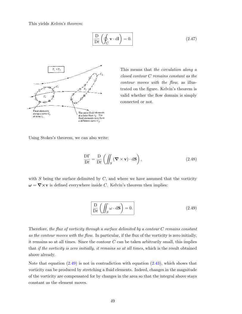
This yields Kelvin’s theorem:
D
Dt
(˛C
v · dl
)= 0. (2.47)
This means that the circulation along a
closed contour C remains constant as the
contour moves with the flow, as illus-
trated on the figure. Kelvin’s theorem is
valid whether the flow domain is simply
connected or not.
Using Stokes’s theorem, we can also write:
DΓ
Dt=
D
Dt
(¨S
(∇× v) · dS
), (2.48)
with S being the surface delimited by C, and where we have assumed that the vorticity
ω =∇×v is defined everywhere inside C. Kelvin’s theorem then implies:
D
Dt
(¨Sω · dS
)= 0. (2.49)
Therefore, the flux of vorticity through a surface delimited by a contour C remains constant
as the contour moves with the flow. In particular, if the flux of the vorticity is zero initially,
it remains so at all times. Since the contour C can be taken arbitrarily small, this implies
that if the vorticity is zero initially, it remains so at all times, which is the result obtained
above already.
Note that equation (2.49) is not in contradiction with equation (2.43), which shows that
vorticity can be produced by stretching a fluid elements. Indeed, changes in the magnitude
of the vorticity are compensated for by changes in the area so that the integral above stays
constant as the element moves.
49

The figure illustrates Kelvin’s theorem. A
vortex line associated with a fluid element
is a line that points in the direction of
ω = ∇×v, and it is therefore perpendic-
ular to the streamline associated with that
fluid element. A vortex tube is a bundle
of vortex lines. A consequence of Kelvin’s
theorem is that the vortex lines/tubes move
with the fluid.
A vortex line attached to some fluid element remains attached to that fluid element
as it moves with the flow. We say that the vorticity moves with the fluid. This is
Helmholtz’s theorem.
A consequence of equation (2.49) is that a vortex line cannot end in the fluid: it either
terminates at the boundaries or forms a closed curve. (If it ended in the fluid, there would
be no flux of vorticity through the surface delimited by a closed contour, so the flux of
vorticity would not be constant.)
We now examine the particular case of a two–dimensional flow in which v = vxx+vyy,
with x and y being the unit vectors in the x and y directions, respectively, and where vx
and vy do not depend on z. Then ω is in the z–direction and (ω ·∇) v = ω (∂v/∂z) = 0.
ThereforeDω
Dt= 0 for a 2D ideal flow , (2.50)
assuming that it is subject to a conservative body force and it has a density ρ which is
constant throughout. This means that the vorticity of a fluid element is conserved as the
element moves with the flow. If the flow is steady, then the vorticity equation becomes
(v ·∇)ω = 0, which means that the vorticity is conserved along streamlines.
2.5 Conservation of energy and Bernoulli’s theorem
In the same way that the equation of motion in Mechanics leads to an equation expressing
conservation of energy, the Navier–Stokes equation can be re–written to express conserva-
tion of energy in a moving fluid. In an ideal fluid, this leads to the so–called Bernoulli’s
theorem.
2.5.1 Conservation of energy in an incompressible Newtonian fluid
The kinetic energy per unit volume is ρv2/2 ≡ ρv ·v/2, and its Eulerian rate of change is:
∂
∂t
(ρv2
2
)= ρv · ∂v
∂t+v2
2
∂ρ
∂t≡ ρvi
∂vi∂t
+v2
2
∂ρ
∂t.
Substituting ρ∂vi/∂t using equation (2.20), we obtain:
50
∂
∂t
(ρv2
2
)= −1
2ρvj
∂v2
∂xj− vi
∂p
∂xi+ vi
∂σij∂xj
− ρvigi +v2
2
∂ρ
∂t. (2.51)
Using the fact that the fluid is incompressible, so that ∂vi/∂xi = 0, and the mass conser-
vation equation ∂ρ/∂t = −vi∂ρ/∂xi, the equation above can be written as:
∂
∂t
(ρv2
2
)= − ∂
∂xj
(1
2ρv2vj
)− ∂
∂xi(vip) +
∂
∂xj(viσij)− σij
∂vi∂xj− ρvigi. (2.52)
Each of the first three terms on the right–hand–side is a divergence. We now integrate
this equation over a fixed volume V and use the divergence theorem to transform these
three terms into a surface integral:
d
dt
˚V
ρv2
2dV = −
"S
1
2ρv2v · dS−
"Spv · dS +
"SviσijnjdS
+
˚V
fvol · v dV −˚
Vσij
∂vi∂xj
dV, (2.53)
where fvol ≡ ρg is the gravitational force (to which we may add any other body force acting
on the fluid) and nj is the j–component of the unit vector n normal to the surface. Since
the volume is fixed, we have moved the time derivative outside the integral on the left–
hand–side. This equation means that the rate of change of kinetic energy in the volume
V (term on the left–hand–side) is equal to the sum of the terms on the right–hand–side
which are, in the order they are written:
• flux of kinetic energy advected by the fluid across the surface,
• work done per unit time by the pressure force −pdS exerted on the surface,
• work done per unit time by the viscous force exerted on the surface (the i–component
of the viscous force per unit surface area is σijnj , as given by eq. [2.1]),
• work done per unit time by the gravitational force (or any other body force) exerted
on the volume,
• irreversible energy dissipation rate due to viscosity10; we denote this term D.
The work done by the pressure and gravitational forces leads to a rate of change of kinetic
energy which is stored as potential energy and returned without loss to the system when
the forces are removed. By contrast, the work done by viscous forces is only partially
10The fact that this term leads to energy dissipation can be shown by writing the equation of conservation
of entropy, which takes the form:
ρTDs
Dt= σij
∂vi∂xj
,
where s is the entropy and T is the temperature (e.g., Landau & Lifshitz, Chapter V, §49).
51

returned when the forces are removed: an amount D of energy per unit time is irreversibly
transformed into thermal energy (i.e. energy of ordered motion transferred into disordered
motion).
As the stress tensor is symmetrical, and making the sum over repeated indices explicit,
we can write:
σij∂vi∂xj
=
3∑i=1
3∑j=1
1
2(σij + σji)
∂vi∂xj
=
3∑i=1
3∑j=1
1
2σij
∂vi∂xj
+
3∑j=1
3∑i=1
1
2σij
∂vj∂xi
,
where we have interchanged the indices in the second double sum. For a Newtonian
incompressible fluid, σij is given by equation (2.13), and therefore the rate of energy
dissipation can be written as:
D =
˚Vσij
∂vi∂xj
dV = 2η
˚Ve2ij dV , (2.54)
where summation over i and j means that e2ij = e2
11 +e222 +e2
33 +2e212 +2e2
13 +2e223, since eij
is symmetrical. As D expresses an irreversible dissipation of energy, it has to be positive,
which implies η > 0. Not surprisingly, D is related to the rate of change of the deformation
eij of fluid elements. In a solid, the energy D may be stored as potential energy of elastic
deformation and returned to the system when the deformation is removed. However, in a
fluid, this corresponds to an irreversible loss of kinetic energy.
It is interesting to compare the work Wsurf done by the viscous forces which are exerted
on the surface of a volume V with the work Wvol done by the resultant viscous force per
unit volume given by equation (2.14). They can be written as:
Wsurf =
"SviTidS =
"SviσijnjdS =
˚V
∂
∂xj(viσij) dV,
and:
Wvol =
˚Vvi∂σij∂xj
dV = Wsurf −D.
Navier–Stokes equation (2.20) multiplied by vi and integrated over a volume V yields:
˚Vvi
DviDt
dV = Wp +Wvol +Wg,
where Wp and Wg are the work done by pressure and gravitational forces, respectively
(note that here the work done by surface pressure forces is equal to the work done by
the resultant pressure force per unit volume, as the fluid is incompressible). Therefore,
the rate of change of kinetic energy is related to Wvol. However, this quantity does not
represent the work done by viscous forces when the velocities vary across the volume,
because in that case the surface forces are exerted at points which move with different
velocities. If the velocity were uniform throughout the volume, Wvol would be equal to
Wsurf and there would be no dissipation. In that case, the work done by viscous forces
results only in a change of the bulk velocity of the volume. However, when the velocity is
52

non uniform, Wsurf = Wvol +D, where Wvol is the part of the work that changes the bulk
velocity of the fluid and D is the part that deforms the volume without changing its bulk
velocity.
2.5.2 Conservation of energy in a steady ideal fluid: Bernoulli’s theorem
We now focus on the particular case of an ideal fluid, which is both incompressible and
inviscid (ν = 0). Although we could just use the equations above with σij = 0, we
obtain more general results by re–deriving the conservation energy equation from Euler’s
equation (2.30). Writing the gravitational acceleration as the gradient of a potential,
g = −∇χ, and assuming ρ to be constant throughout the fluid, this equation becomes:
ρ∂v
∂t+ ρ (∇×v)×v = −∇
(1
2ρv2 + p+ ρχ
). (2.55)
(eq. [2.40]) with ν = 0 and in which we have replaced ω by ∇×v).
Bernoulli streamline theorem:
We now consider a steady flow and take the dot product of equation (2.55) with v. As the
vector (∇×v)×v is perpendicular to v, this yields:
(v ·∇)
(1
2ρv2 + p+ ρχ
)= 0, (2.56)
which means that the quantity
H =1
2ρv2 + p+ ρχ is constant along streamlines. (2.57)
This is called Bernoulli’s theorem, and is valid for a steady, inviscid and incompressible fluid
in which ρ is constant throughout the fluid. It implies that, if the gravitational potential
is constant along a streamline, the flow accelerates when the pressure decreases11.
The quantity ρv2/2, which is the kinetic energy per unit volume, has the dimensions
of a pressure and is called the dynamic pressure, and p+ ρv2/2 is the total pressure. The
fact that H is constant along streamlines can be understood by noting that, when the
pressure p is increasing in the direction of the flow, fluid elements have to do work against
11Bernoulli’s theorem is responsible for the cavitation phenomenon, which is the formation of vapor
bubbles in a fluid when the velocity increases sufficiently that the pressure drops down to the saturation
vapor limit. This happens for example behind the blade of a rapidly rotating ship propeller. Due to the
higher pressure of the surrounding medium, the bubbles subsequently collapse, emitting large amplitude
shock waves which release energy locally and damage the blades of the propeller. This emission of shock
waves enables to detect military submarines. Cavitation bubbles are also used in a range of medical
procedures to deposit energy non–intrusively, for example to target cancer cells or break kidney stones.
Cavitation bubbles are also an efficient tool for Mantis shrimps to catch their preys: the rapid motion of
the claws generates bubbles which, when they subsequently collapse, produce a measurable force on the
prey that can be enough to kill it.
53

the pressure gradient and therefore loose kinetic energy. In the opposite case, when the
pressure p is decreasing, fluids elements gain kinetic energy. The quantity H is often
referred to as the total enthalpy per unit volume.
Bernoulli’s theorem for irrotational flow:
In an irrotational flow, ∇×v = 0, and v can be written as the gradient of a velocity
potential φ: v =∇φ (see section 1.8.1). Therefore, equation (2.55) implies:
ρ∂φ
∂t+
1
2ρv2 + p+ ρχ = C(t), (2.58)
where C is a function of time only. The quantity on the left–hand side is therefore constant
throughout the whole fluid at any given time. Since any function of time can be added to
φ without changing the velocity, the function C(t) can be subsumed into ∂φ/∂t by adding
(1/ρ)´ tt0C(t′)dt′ to φ, where t0 is an arbitrary constant. Therefore, Bernoulli’s theorem
becomes:
ρ∂φ
∂t+
1
2ρv2 + p+ ρχ = 0. (2.59)
If the flow is steady, then
H =1
2ρv2 + p+ ρχ is constant throughout the whole fluid, (2.60)
but here the constant is not necessarily zero. This is an extension of Bernoulli’s theorem
which is valid for a steady, inviscid, incompressible and irrotational fluid in which ρ is
constant throughout.
2.6 Examples of viscous flows and very viscous flows
Couette, Poiseuille and Stokes flows are studied in Problem Set 2.
54

Chapter 3
Potential flows
A potential flow is a flow which is both inviscid and irrotational. The name comes from the
fact that, in an irrotational flow, the velocity can be written as the gradient of a velocity
potential.
In the previous chapter, we have established Kelvin’s theorem, which states that if
an inviscid flow has no vorticity initially, it has no vorticity at all subsequent times and
therefore remains a potential flow (provided the external force is derivable from a potential
and the mass density is constant throughout the fluid). In particular, a flow which is at
rest initially is a potential flow.
There is a difficulty near a solid boundary though, as may occur if an object is immersed
in the flow. As we have already pointed out in section 2.3.1, viscosity cannot be ignored
near a rigid boundary, even if it can be neglected in the interior of the fluid. The large stress
that results from the flow velocity adjusting to the boundary condition creates a boundary
layer in which viscous effects are important. Potential flow theory does not apply in such
boundary layers, which will be studied in the next chapter. However, the flow moving
past a solid object may still be calculated using the potential flow approximation in the
outer regions if the Reynolds number is large there (larger than about 25), and matched
to boundary layer approximations near the object.
In this chapter, we will be concerned with irrotational high Reynolds number flows,
approximated as inviscid. We will also limit our study to incompressible fluids.
Important applications of potential flow theory include water waves and outer flows
(away from the boundary layers) around aerofoils, which are the cross–sectional shape of
an object designed to generate lift when moving through a fluid, like a wing, blade or sail.
The study of the motion of air past an aerofoil is called aerodynamics. As pointed out
in section 2.2.4, air is approximated to be incompressible for Mach numbers below 0.3.
Therefore, although incompressible potential flow theory would not apply to commercial
aircrafts, which cruise at speeds of Mach larger than 0.8, it is important for low–speed
aerodynamics. The Reynolds number Re = UL/ν depends on the characteristic velocity
U of the flow and on the characteristic lengthscale L over which parameters vary. In the
case of aerodynamics, L is the size of the aerofoil. Therefore, high Reynolds numbers
are achieved for high–speed flows around larger objects. In the case of waves, L is the
55

wavelength, so potential theory applies to large scale disturbances.
3.1 General properties of potential flows
In this chapter, we make the following assumptions:
• the flow is inviscid (ν = 0),
• the flow is irrotational (∇×v = 0),
• the flow is incompressible (∇ · v = 0),
• ρ is uniform throughout the fluid,
• the external force is gravity with the gravitational acceleration given by g = −∇χ.
The condition ∇×v = 0 implies that the velocity can be written as the gradient of
a velocity potential φ: v = ∇φ. As pointed out in section 1.8.1, φ is a single–valued
function of position only if the flow domain is simply connected. Also, φ is not uniquely
defined by the equation above: any function of time can be added to a solution without
modifying v.
Incompressibility yields:
∇ · v = ∇2φ = 0 , (3.1)
which means that φ satisfies Laplace’s equation. The boundary conditions for φ follow
from the boundary conditions for v. If the boundary is rigid, equation (2.31) implies that
the normal derivative of φ on the surface (that is to say, the derivative in the direction
of the normal to the boundary) is equal to the normal component of the velocity of the
boundary itself:∂φ
∂n
)surface
= vn,boundary. (3.2)
If the boundary is an interface between two fluids, then equation (2.33) implies:
∂φ
∂n
)fluid 1, surface
=∂φ
∂n
)fluid 2, surface
. (3.3)
The no–slip condition does not apply here as the fluid is inviscid.
It can be shown that, within a simply connected flow domain, Laplace’s equation has
a unique solution in the two following cases: (i) the flow domain is bounded and the
boundary condition (3.2) is satisfied at each point of the boundary, (ii) the flow domain
is not bounded but the boundary condition (3.2) is satisfied at any rigid surface and the
velocity matches that of the fluid at infinity (e.g., flow moving past a sphere).
If the flow domain is not simply connected, other conditions have to be added for the
potential to be determined uniquely.
Calculating φ from Laplace’s equation and then v from ∇φ is much easier than cal-
culating v directly from Euler’s equation, because Laplace’s equation is linear whereas
56

Euler’s equation contains the non–linear term (v ·∇) v. Once the velocity has been ob-
tained, the pressure can be calculated from Euler’s equation (2.30), which we recall here:
ρ∂v
∂t+ ρ (v ·∇) v = −∇p+ ρg. (3.4)
We also recall Bernoulli’s theorem (2.59), as satisfied by incompressible potential flows:
ρ∂φ
∂t+
1
2ρv2 + p+ ρχ is constant throughout the whole fluid. (3.5)
Finally, as we have seen in section 1.8.3, if the flow is two dimensional, as it is also
incompressible, we can define a stream function ψ such that:
vx =∂ψ
∂y, and vy = −∂ψ
∂x, (3.6)
in cartesian coordinates (x, y) or:
vr =1
r
∂ψ
∂θ, and vθ = −∂ψ
∂r. (3.7)
in polar coordinates (r, θ). The lines ψ = constant are streamlines.
Like φ, ψ is not uniquely defined by the equations above: any gradient (in addition to any
function of time) can be added to a solution without modifying v.
Since the flow is irrotational, and noting z the unit vector in the z–direction:
∇×v = −∇2ψ z = 0 , (3.8)
which means that ψ satisfies Laplace’s equation in a two dimensional potential flow.
3.2 Simple potential flows
Because Laplace’s equation is linear, different solutions for φ (and ψ in two dimensions) can
be superposed to yield new and more complex solutions. This is why it is worth studying
very simple potential flows which may not be very realistic, but can be superposed to
construct more interesting flows.
3.2.1 Uniform parallel flows
This is a flow such that v = U x where U is a constant and x is the unit vector along the
x–axis. The vorticity is clearly zero for this flow. The condition v =∇φ then implies:
φ = Ux. (3.9)
If the flow is two dimensional, then equations (3.6) yield:
ψ = Uy. (3.10)
It is easy to verify in this simple example that ψ = constant, that is to say y = constant,
is the equation of the streamlines and that the streamlines and equipotential lines (given
by φ = constant) are perpendicular to each other.
57

3.2.2 Line vortex flow
This a two dimensional flow such that, in polar coordinates:
v =Γ
2πrθ, (3.11)
where Γ is a constant, called the strength of the vortex, and θ is the unit vector in the
azimuthal direction. The vorticity is:
ω =∇×v =1
r
∂ (rvθ)
∂rz = 0.
As already calculated in section 1.8.1, the velocity
potential is given by:
φ =Γθ
2π, (3.12)
which is a multi–valued function of position.
We obtain ψ by integrating equations (3.7):
ψ = − Γ
2πln
r
r0, (3.13)
where we have added a constant to make the argument of the ln dimensionless (as ψ is
defined within an arbitrary constant).
As seen in section 1.8.2, the circulation is defined as:
Γ =
˛C
v · dl,
and, for an irrotational flow, it is the same round all simple contours enclosing the origin.
It was noted in section 1.8.2 that, for a line vortex flow, the circulation of the velocity
around a contour centered at the origin is non zero, even though the vorticity is zero. This
is because the flow domain is not simply connected, due to the singularity at r = 0. In
other words, since the vorticity is not defined at r = 0, Stokes’s theorem does not apply.
One way around this difficulty is to define ω as a Dirac delta function at the origin:
ω(r, θ) = Γδ(0)z, (3.14)
so that: ˆ +∞
r=0
ˆ 2π
θ=0ωrdrdθ = Γ,
and Stokes’s theorem applies. This is really what is meant by line vortex: the vorticity is
non zero only along a line.
58
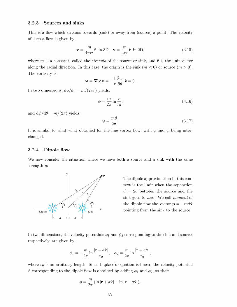
3.2.3 Sources and sinks
This is a flow which streams towards (sink) or away from (source) a point. The velocity
of such a flow is given by:
v =m
4πr2r in 3D, v =
m
2πrr in 2D, (3.15)
where m is a constant, called the strength of the source or sink, and r is the unit vector
along the radial direction. In this case, the origin is the sink (m < 0) or source (m > 0).
The vorticity is:
ω =∇×v = −1
r
∂vr∂θ
z = 0.
In two dimensions, dφ/dr = m/(2πr) yields:
φ =m
2πln
r
r0, (3.16)
and dψ/dθ = m/(2π) yields:
ψ =mθ
2π. (3.17)
It is similar to what what obtained for the line vortex flow, with φ and ψ being inter-
changed.
3.2.4 Dipole flow
We now consider the situation where we have both a source and a sink with the same
strength m.
The dipole approximation in this con-
text is the limit when the separation
d = 2a between the source and the
sink goes to zero. We call moment of
the dipole flow the vector p = −mdxpointing from the sink to the source.
In two dimensions, the velocity potentials φ1 and φ2 corresponding to the sink and source,
respectively, are given by:
φ1 = −m2π
ln|r− ax|r0
, φ2 =m
2πln|r + ax|r0
,
where r0 is an arbitrary length. Since Laplace’s equation is linear, the velocity potential
φ corresponding to the dipole flow is obtained by adding φ1 and φ2, so that:
φ =m
2π(ln |r + ax| − ln |r− ax|) .
59

Using a/r 1, to first order in a/r we obtain:
φ =m
2π
2a cos θ
r=p cos θ
2πr= −p · r
2πr, (3.18)
where r is the unit vector in the radial direction. The velocity is then calculated from the
gradient of φ:
vr =∂φ
∂r= −p cos θ
2πr2, vθ =
1
r
∂φ
∂θ= −p sin θ
2πr2. (3.19)
The figure shows the streamlines in blue and
the equipotential (lines of constant φ) in
red. This is similar to the calculation of
the electrostatic potential due to an electric
dipole, as expected since in both cases the
potential satisfies Laplace’s equation.
3.2.5 Flow around a circular cylinder
We consider a flow moving past an infinite cylinder perpendicularly to its axis.
Far away from the cylinder, the flow velocity is
v = U x. Since there is no dependence on the
coordinate along the axis of the cylinder, this is
a two dimensional problem in the (x, y), or (r, θ),
plane. We note R the radius of the cylinder cross–
section.
Because of the presence of the cylinder, the flow domain is not simply connected (a contour
encircling the cylinder cannot be shrunk to zero continuously while staying in the domain).
However, it could be shown that the solution to Laplace’s equation satisfying the boundary
condition (3.2) at the surface of the cylinder and matching the velocity at infinity is unique
if we specify the circulation around the cylinder. Below, we therefore examine two different
cases corresponding to two different circulations.
Like in electrostatics, the velocity potential can be written as a multipole expansion.
The general solution of Laplace’s equation in two dimensions, using polar coordinates, is:
φ(r, θ) = (a0 + b0 ln r) (A0 +B0θ) +
∞∑n=1
[An cos (nθ) +Bn sin (nθ)](anr
n + bnr−n) .
(3.20)
60

We recognise the following terms: A0b0 ln r corresponds to a sink or a source, a0B0θ corre-
sponds to a line vortex, A1a1r cos θ corresponds to a uniform flow, A1b1 cos θ/r corresponds
to a dipole flow.
Cylinder with no circulation:
If there is no circulation around the cylinder, then the term corresponding to the line
vortex in the above expansion of φ is zero. Since there is also no sink nor source in the
fluid, the first non zero term in the expansion is the n = 1 dipole term. Since the flow
velocity at infinity is proportional to cos θ, we set B1 = 0 and look for solutions under the
form:
φ =
(ar +
b
r
)cos θ.
If we can find a solution under this form which satisfies the boundary conditions, then
this is the solution as we have also specified the circulation and therefore the solution is
unique. At infinity, we have a uniform flow for which φ = Ux = Ur cos θ as shown in
section 3.2.1. Therefore a = U . At r = R, vr = ∂φ/∂r has to be zero to satisfy the
boundary condition (3.2). Therefore U − b/R2 = 0, which yields b = UR2. The solution
is then:
φ = U
(1 +
R2
r2
)r cos θ, (3.21)
which is the sum of a uniform parallel flow and a dipole flow. The gradient of φ then gives
the velocity:
vr = U
(1− R2
r2
)cos θ, vθ = −U
(1 +
R2
r2
)sin θ. (3.22)
There are two stagnation points, where the velocity vanishes: (R, 0) and (R, π).
To obtain the equations of the streamlines (shown
on the figure), we can also calculate the stream
function ψ by integrating equations (3.7), which
yields:
ψ = U
(1− R2
r2
)r sin θ. (3.23)
The streamline ψ = 0 is made of the two
semi–infinite lines along the x–axis plus the cir-
cumference of the cylinder. As we have discussed
in section 2.3, in a two dimensional flow, a rigid
boundary is always a streamline as the velocity
has no normal component at the boundary.
(Credit: https://www.ecourses.ou.edu)
61

The pressure is obtained from Bernoulli’s theorem (3.5) applied to a steady flow, which
states that ρv2/2 + p is constant throughout the whole fluid, as χ is uniform. If we note
p0 the pressure at infinity, then the pressure at the surface of the cylinder is given by:
p(R, θ) = p0 +1
2ρU2 − 1
2ρv2(R, θ) = p0 +
1
2ρU2
(1− 4 sin2 θ
). (3.24)
In this figure, the streamlines correspond to
the black curves, the equipotential lines to
the white curves, and pressure is indicated
by the colors (red and blue are high and
low pressure, respectively).
(Credit: Wikipedia)
Because of the symmetry of the pressure, there is no net force acting on the cylinder.
This conclusion can be shown to hold for any object, not just a cylinder. This is known
as the d’Alembert paradox, as obviously common experience is that any object moving
relative to a fluid is subject to a significant resistance, or drag1. A solution to this paradox
will be presented in the next chapter.
Cylinder with circulation:
If the cylinder rotates around its axis, the relative motion of the fluid at the surface
results in a finite circulation around the cylinder. Note that, as shown in section 1.8.2, for
an irrotational flow, the circulation is the same round all simple contours enclosing the
1D’Alembert did this calculation in 1752 as a prize problem for the Berlin Academy of Science. The
motion of a body relative to an inviscid and incompressible flow was important to understand the design
of boats. The result however, indicating that there would be no drag, discredited completely mathematical
fluid mechanics, and d’Alembert did not get the prize. This episode prompted the words of Sir Hinshelwood
taken as an epigraph for these notes. Prandtl proposed a resolution of the paradox in 1904, when he found
that even a very small viscosity would result in the creation of a boundary layer at the surface of the
object in which viscous forces produce a drag. This is largely accepted as the right way of accounting
for the drag force, as it is completely supported by experimental observations and mathematical analysis.
However, there is no rigorous mathematical proof of this process and another solution to the paradox has
been proposed recently, in which the drag is produced by the turbulence which results from the inviscid
potential flow being unstable. No viscosity is required in that case.
62
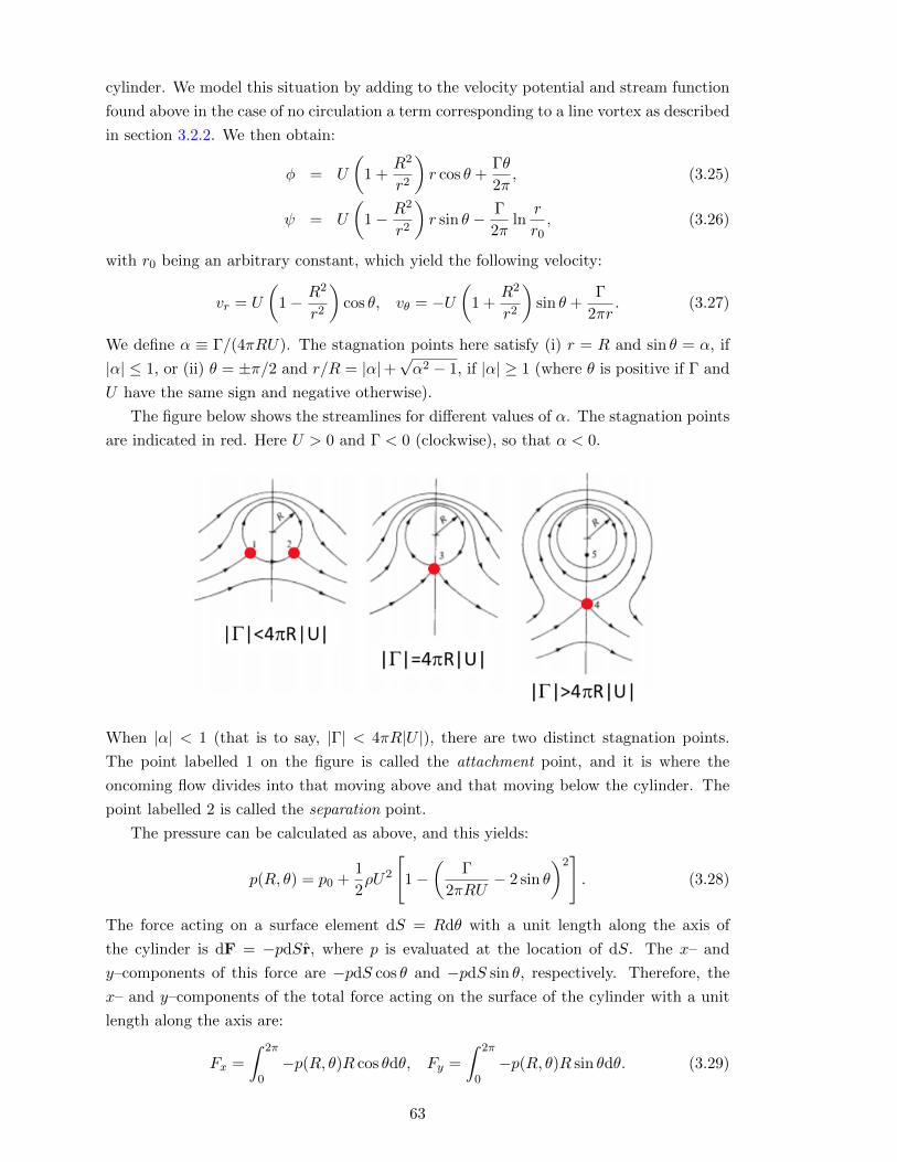
cylinder. We model this situation by adding to the velocity potential and stream function
found above in the case of no circulation a term corresponding to a line vortex as described
in section 3.2.2. We then obtain:
φ = U
(1 +
R2
r2
)r cos θ +
Γθ
2π, (3.25)
ψ = U
(1− R2
r2
)r sin θ − Γ
2πln
r
r0, (3.26)
with r0 being an arbitrary constant, which yield the following velocity:
vr = U
(1− R2
r2
)cos θ, vθ = −U
(1 +
R2
r2
)sin θ +
Γ
2πr. (3.27)
We define α ≡ Γ/(4πRU). The stagnation points here satisfy (i) r = R and sin θ = α, if
|α| ≤ 1, or (ii) θ = ±π/2 and r/R = |α|+√α2 − 1, if |α| ≥ 1 (where θ is positive if Γ and
U have the same sign and negative otherwise).
The figure below shows the streamlines for different values of α. The stagnation points
are indicated in red. Here U > 0 and Γ < 0 (clockwise), so that α < 0.
When |α| < 1 (that is to say, |Γ| < 4πR|U |), there are two distinct stagnation points.
The point labelled 1 on the figure is called the attachment point, and it is where the
oncoming flow divides into that moving above and that moving below the cylinder. The
point labelled 2 is called the separation point.
The pressure can be calculated as above, and this yields:
p(R, θ) = p0 +1
2ρU2
[1−
(Γ
2πRU− 2 sin θ
)2]. (3.28)
The force acting on a surface element dS = Rdθ with a unit length along the axis of
the cylinder is dF = −pdSr, where p is evaluated at the location of dS. The x– and
y–components of this force are −pdS cos θ and −pdS sin θ, respectively. Therefore, the
x– and y–components of the total force acting on the surface of the cylinder with a unit
length along the axis are:
Fx =
ˆ 2π
0−p(R, θ)R cos θdθ, Fy =
ˆ 2π
0−p(R, θ)R sin θdθ. (3.29)
63

The force in the x–direction, which is called the drag, is zero, like in the case of no
circulation.
However, there is a non zero force in the y-direction, which is called the lift. It is due to
the sin θ term in the expression for p:
Fy =
ˆ 2π
0−ρUΓ
πsin2 θdθ = −ρUΓ. (3.30)
In the context of a rotating object immersed in a fluid, the lift is also called the Magnus
force. It is a well–known effect in tennis or football, as it leads to the swerving of balls
which are hit with spin. On the figure above, where U > 0 and Γ < 0 (clockwise), Fy > 0
so that the cylinder is pushed upwards.
The direction of the lift can be understood in the following way:
Because the velocity of the parallel
flow is in the same direction as that
of the line vortex above the cylinder,
and in the opposite direction below
the cylinder, the flow velocity is
larger above than below the cylinder.
(This results in the streamlines being closer to each other above than below the cylinder,
as seen in Problem Set 1). Bernoulli’s theorem then implies that the pressure is larger
below than above the cylinder, which results in an upwards force on the cylinder.
It is important to note that the vertical
pressure gradient is due to the fact that
the streamlines are curved, as illustrated
on the figure.
The change of direction of the velocity v yields a centripetal acceleration v2/r per unit
mass, where r is the local radius of curvature, which can only be generated by the pres-
sure force ∂p/∂n, where n is the coordinate in the direction normal to the streamline.
Therefore pressure decreases towards the centre of curvature. (This effect is the reason
why the pressure at the core of a tornado is very low, and objects get ’sucked’ into the
sky.) In the case of the cylinder with circulation, the streamlines are curved in such a
way that pressure decreases when we approach the cylinder moving vertically either from
the top or from the bottom. However, because both the curvature radius is smaller and
the velocity is larger above the cylinder, the drop in pressure is more significant above
than below the cylinder. The lift is therefore due to an asymmetry in the curvature of the
streamlines. Such a situation, which here is the result of the rotation of the cylinder, may
64

also be produced by a stationary cylinder with a sharp–edged flap at the separation point
or by a wing2.
This figure illustrates how the Mag-
nus effect can be used on a ship to
reduce fuel comsuption.
Although it is straightforward to calculate the lift in the simple case of a flow past
a cylinder by directly solving for the velocity and pressure, it is much more difficult to
do so for a more complicated aerofoil. However, in two dimensions, techniques based on
complex variables can be used to map the flow past a cylinder into the same flow past a
different object. This is the object of the next section.
3.3 Complex velocity potential
In this section, we consider an incompressible and irrotational two dimensional flow.
3.3.1 Cauchy–Riemann equations
The velocity may be written as a function of either the potential velocity or the stream
function:
vx =∂φ
∂x=∂ψ
∂y, and vy =
∂φ
∂y= −∂ψ
∂x. (3.31)
The functions φ(x, y) and ψ(x, y) then satisfy the Cauchy–Riemann equations, so that the
complex potential, defined as:
w(z) = φ(x, y) + iψ(x, y), (3.32)
with z = x + iy, is differentiable (see appendix A). The derivative of w can then be
calculated by keeping y constant:
dw
dz=∂φ
∂x+ i
∂ψ
∂x= vx − ivy. (3.33)
2A very good description of the lift on aerofoils is given in How do wings work?, H. Babinsky, 2003,
Physics Education, 38, 497. In this article, the author shows that the ’popular’ explanation for the lift that
fluid particles flowing across the top and the bottom surfaces must reach the trailing edge of the aerofoil
at the same time, which results in higher speed and therefore lower pressure at the top, is wrong.
65

These results also apply in polar coordinates, using z = reiθ. Both φ and ψ, and therefore
w, may be multi–valued functions. However, by specifying the values the function can take
(which is known as specifying a branch of the function), we can make it single–valued. Since
it is also differentiable, it then becomes an analytic function.
Cauchy–Riemann equations also imply that both φ and ψ satisfy Laplace’s equation, as
already pointed out in section 3.1.
3.3.2 Complex potential of a flow past a cylinder
In the absence of circulation, we have found above that the potential and stream function
of a flow past a cylinder are: φ = U(r +R2/r
)cos θ and ψ = U
(r −R2/r
)sin θ (eq. [3.21]
and [3.23]). Using z = reiθ, we obtain:
w(z) = U
(ze−iθ +
R2
zeiθ
)cos θ + iU
(ze−iθ − R2
zeiθ
)sin θ = U
(z +
R2
z
). (3.34)
For a line vortex, the potential is φ = Γθ/(2π) and ψ = −(Γ/(2π)) ln (r) (eq. [3.12] and
[3.13] where we have taken r0 = 1), so that:
w(z) =Γ
2π(−i ln r + θ) = − iΓ
2π(ln r + iθ) ≡ − iΓ
2πln z, (3.35)
defined up to an additive constant3.
Therefore the complex potential for a flow past a cylinder with circulation Γ is:
w(z) = U
(z +
R2
z
)− iΓ
2πln z. (3.36)
3.3.3 Conformal mapping
This is a technique in which a flow problem (or more generally a Laplace equation problem)
in simple geometries is transformed into more complicated geometries by using an analytic
mapping function that preserves the angles.
We consider a pair of complex variables z = x + iy and Z = X + iY , each defined in
their own complex plane, such that:
Z = f(z) (3.37)
is an analytic function of z. This is a transformation that maps a point (x, y) in the
z–plane into a point (X,Y ) in the Z–plane. The inverse z = F (Z) is also an analytic
function of Z if f ′(z) 6= 0, as F ′(Z) ≡(f−1
)′(Z) = 1/f ′
(f−1(Z)
)≡ 1/f ′ (z) .
3The logarithm of a complex number z = reiθ is defined as follows:
ln(z) = ln r + i (θ + 2πk) ,
where k is an integer. Although this is a multi–valued function, we can specify the branch as −π ≤Im [ln(z)] ≤ π so that the function (called principal value) becomes single–valued.
66
It can be shown that:
At the points in the z–plane where the first derivative of f is non–zero, the transfor-
mation preserves the angles and is called conformal mapping.
This means that two short segments which are perpendicular in the z–plane are mapped
into two short segments which are also perpendicular in the Z–plane. More generally, if
the first non–zero derivative of f at a point z is the nth derivative, then a local angle at z
is multiplied by n when mapped into the Z–plane. (See, e.g., section 4.6 in Acheson for a
proof).
If w(z) = φ(x, y)+iψ(x, y) is the complex potential of a two dimensional incompressible
potential flow in the z–plane, and Z = f(z) is a conformal transformation, then:
W (Z) = w (F (Z)) = Φ(X,Y ) + iΨ(X,Y )
is an analytic function of Z. It follows that Φ and Ψ satisfy the Cauchy–Riemann relations,
which implies that they satisfy Laplace’s equation4, and that VX(X,Y ) = ∂Φ/∂X =
∂Ψ/∂Y and VY (X,Y ) = ∂Φ/∂Y = −∂Ψ/∂X represent the velocity components of an
incompressible potential flow in the Z–plane, with again dW/dZ = VX− iVY . In addition,
since W (Z) = w (F (Z)), the value of φ at (x, y) is the same at that of Φ at (X,Y ) when
those two points are related by z = F (Z), with similar result for ψ and Ψ. This implies that
streamlines in the (x, y)–plane are mapped into streamlines in the (X,Y )–plane through
this transformation. Furthermore, as rigid boundaries are themselves streamlines, they
too map into rigid boundaries in the (X,Y )–plane.
In other words, if we know the streamlines and equipotentials of a flow in a given
geometry, we can obtain the streamlines and equipotentials corresponding to any
conformal mapping of this geometry.
Note that, since W (Z) = w (F (Z)), the streamline ψ(x, y) = C1, for example, trans-
forms into the streamline Ψ(X,Y ) = C1. We would still obtain a flow in the Z–plane
with W (Z) = 2w (F (Z)), for example, but that would lead to the velocity satisfying
different boundary conditions. The complex potential in the Z–plane is defined to be
W (Z) = w (F (Z)) because, in the case of the flow past an aerofoil, as studied below, the
velocity satisfies the same boundary condition at infinity in both the z and Z–planes.
4The transformation needs to be conformal for Laplace’s equation in the z–plane to be transformed
into Laplace’s equation in the Z–plane because, e.g.,
∇2Φ =1
|f ′(z)|2∇2φ,
which requires f ′(z) 6= 0.
67

We now illustrate conformal mapping with the simple case of a uniform parallel flow.
We consider the transformation Z = f(z) =√z, with the inverse being z = F (Z) = Z2.
Writing z = |z|eiθ, with −π ≤ θ ≤ π, f(z) has two branch functions, f+(z) =√|z|eiθ/2
and f−(z) = −√|z|eiθ/2. Each of these functions is single–valued. However, they are not
continuous at points along the axis θ = ±π (x ≤ 0 axis), which is called the branch cut.
The end–point of the branch cut, which is z = 0 and where f+ and f− are both 0, is
called a branch point and is a singularity. If we exclude the branch cut, then each of these
functions is analytic. In what follows we consider f+, which is called the principal value.
Then the z–plane is mapped into the the right half of the Z–plane, in the way illustrated
in the figure below, where the thick dashed black line indicates the branch cut :
For a uniform parallel flow, the potential and stream function are given by φ(x, y) = Ux
and ψ(x, y) = Uy (see eq.[3.9] and [3.10]). Therefore, the complex potential is w(z) =
U (x+ iy) = Uz. For simplicity we take U = 1. Using the transformation f+(z), the
complex potential in the Z–plane can be written as:
W (Z) = w(Z2)
= Z2 = (X + iY )2 = X2 − Y 2 + 2iXY.
Therefore Φ(X,Y ) = X2 − Y 2 and Ψ(X,Y ) = 2XY . In the z-plane, the streamlines
ψ = y = constant are horizontal lines, and the equipotentials φ = x = constant are vertical
lines. In the Z-plane, the streamlines become Ψ = 2XY = constant, which are hyperbo-
las with the coordinate axes as asymptotes, and the equipotentials are Φ = X2 − Y 2 =
constant, which are hyperbolas with either the X– or Y –axis as axis of symmetry. The
figure below shows the streamlines in red and the equipotentials in blue for this flow in
the z– and Z–planes. The colored dots illustrate how different points are mapped. We
can think of the thick black line just above the x–axis in the z–plane as a rigid boundary,
which maps into the thick black rigid boundary shown in the Z–plane. Therefore, this
mapping has transformed a uniform parallel flow into a flow in a right–angle corner, as
could be confirmed by calculating directly the potential and stream function in this latter
case.
68

We notice on the figure above that the streamlines and equipotentials, which are per-
pendicular in the z–plane, as still perpendicular in the Z–plane, as they should from the
discussion in section 1.8. The transformation is indeed conformal as f ′ does not vanish,
and conformal mapping always preserves the angles.
We now discuss a transformation which is very important in the context of aerody-
namics.
3.3.4 The Joukowski transformation
The Joukowski transformation enables a two dimensional flow around a cylinder to be
mapped onto a two dimensional flow around the wing of an airplane. It is given by:
Z = f(z) = z +c2
z, (3.38)
where c is a real number. The inverse is then:
z = F (Z) =1
2
(Z +
√Z2 − 4c2
), (3.39)
where we have not inserted ± in front of the square root as it is understood to have two
branch functions. To make this function continuous we exclude the branch cut which
is the segment along the X–axis between −2c and 2c. We also make it single–valued
by selecting the principal value of the square root. Therefore z ∼ Z when |Z| is large.
Excluding Z = ±2c is equivalent to excluding z = ±c, which are the only points where
f ′(z) = 0. Therefore, the transformation is conformal in the domain which excludes the
branch cut.
Using z = reiθ, the transformation can be written as:
Z = reiθ +c2
re−iθ =
(r +
c2
r
)cos θ + i
(r − c2
r
)sin θ. (3.40)
The real and imaginary parts are equal to X and Y , respectively. Writing cos2 θ+sin2 θ =
1, we then obtain:X2
(r + c2/r)2 +Y 2
(r − c2/r)2 = 1.
If r is a constant, that is to say z moves along a circle of radius r centered at the origin
in the z–plane, then this equation is that of an ellipse. If r = c, Z = 2c cos θ, which is a
69

segment along the X–axis, as illustrated on the figure below:
Here again, we can think of the circle of radius c in the z–plane as a rigid boundary
which maps into a plate segment which is also a rigid boundary in the Z–plane. Let us
consider a uniform parallel flow past this plate. The complex potential for this flow, as
seen above (section 3.3.3), is W (Z) = UZ, with U being the velocity. We can map this
flow back into the flow around the circle in the z–plane:
w(z) = W (f(z)) = U
(z +
c2
z
). (3.41)
This is an elegant way to recover the result we have already obtained above (eq. [3.34]).
3.3.5 Potential flow past a finite plate and the Kutta condition
The complex potential corresponding to a flow past a circle of radius R when there is
a finite circulation is given by equation (3.36). This corresponds to the case when the
oncoming uniform flow is parallel to the x–axis.
If, instead, this flow was coming from below the x–
axis at an angle of attack α, the complex potential
would be obtained from equation (3.36) by changing
θ to θ − α or, equivalently, by changing z = reiθ to
ze−iα. This yields:
w(z) = U
(ze−iα +
R2
zeiα
)− iΓ
2πln z, (3.42)
where we have ignored e−iα in the ln as it amounts to just adding a constant to the
potential. If we now map this flow into the Z–plane using Joukowski transformation (3.38)
with c = R, we get the complex potential W (Z) of a flow incident at an angle α onto a plate
segment, since the angles are preserved. The expression for W (Z) is rather complicated,
so instead of calculating it we derive the velocity components VX and VY in the Z–plane
70

using VX − iVY = dW/dZ. Since W (Z) = w (F (Z)), with z = F (Z), we obtain:
VX − iVY =dw
dz
dz
dZ=
dw
dz
(dZ
dz
)−1
. (3.43)
Using equations (3.38) with c = R and (3.42), this yields:
VX − iVY =
(Ue−iα − UeiαR
2
z2− iΓ
2πz
)z2
z2 −R2. (3.44)
These velocities represent the flow in the Z–plane and therefore need to be expressed as
a function of Z. However, keeping in mind the relation (3.38) between z and Z, we can
get useful information from the expression above.
We see that, if the term inside the brackets in the above equation is non zero, the flow
speed is infinite when z = ±R, which corresponds to Z = ±2R, that is to say the ends of
the plate. We call trailing edge the downstream edge of the plate, located at X = 2R, and
leading edge the upstream edge, located at X = −2R. The velocity at the trailing edge
can be made finite if the term in brackets vanishes for z = R, which implies:
Ue−iα − Ueiα − iΓ
2πR= 0, (3.45)
that is to say:
Γ = −4πRU sinα. (3.46)
This is called the Kutta condition, and its meaning will be discussed in the next section
in the context of more realistic aerofoils. Writing z = R+ ε, with ε R, equation (3.44)
then yields VX → U cosα and VY → 0 when ε → 0. The fluid is therefore parallel to
the plate at the trailing edge. The figure below shows the streamlines around the circle
in the z–plane and around the finite plate in the Z–plane for both the case where there
is no circulation and the case where there is circulation and the condition above it satisfied:
The Kutta condition implies |Γ| < 4πR|U |, so that in the z–plane there are two distinct
stagnation points s and s′ on the surface of the circle (see section 3.2.5), and since dw/dz =
0 when z = R (eq. [3.45]), s′ is on the x–axis when the Kutta condition is met.
71

3.3.6 The Joukowski aerofoil
In the case of the plate considered above, the velocity at the trailing edge is finite when
the Kutta condition is met, but the velocity at the leading edge is still infinite. This is
why flat plates with sharp edges are not used to make aerofoils.
Instead, aerofoils have a rounded leading edge and
a sharp trailing edge, which yields a finite velocity
everywhere, as we are now going to show.
We can generate such an aerofoil by applying
Joukowski mapping on a circle in the z–plane which
center is not at the origin, as illustrated on the figure.
Since z = −a+(R+a)eiϕ along the circle, Joukowski
transformation (3.38) with c = R yields the shape of
the co–called Joukowski aerofoil in the Z–plane as:
Z = −a+ (R+ a)eiϕ +R2
−a+ (R+ a)eiϕ, (3.47)
which is represented on the figure.
The complex potential in the z–plane for an angle of attack α is the same as that given
by equation (3.42) but with z shifted to z+ a and the radius of the circle changed from R
to R+ a:
w(z) = U
[(z + a)e−iα +
(R+ a)2
z + aeiα
]− iΓ
2πln (z + a) . (3.48)
We then redo the same calculation as above to obtain the velocities:
VX − iVY =dw
dz
(dZ
dz
)−1
, (3.49)
where w(z) is now given by equation (3.48) and Z is still given by equation (3.38) with
c = R. This yields:
VX − iVY =
(Ue−iα − Ueiα (R+ a)2
(z + a)2 −iΓ
2π (z + a)
)z2
z2 −R2. (3.50)
The denominator still vanishes at z = ±R, which still corresponds to Z = ±2R. From
equations (3.38) and (3.39), we see that points on the x–axis in the z–plane map into
points on the X–axis in the Z–plane. Therefore, the aerofoil intersect the X–axis at
points given by equation (3.47) with eiϕ = ±1, that is to say at Z = 2R and Z =
−2R(1 + 2a2/(2aR+R2)
). This means that the point Z = −2R is inside the aerofoil,
72

and there is only one point in the flow where the denominator of equation (3.50) vanishes,
which is the trailing edge of the aerofoil. As in the case of the plate, this singularity
is removed if the term in brackets in equation (3.50) vanishes as well for z = R, which
requires:
Γ = −4π(R+ a)U sinα. (3.51)
This is the Kutta condition for the Joukowski aerofoil. As above, writing z = R+ ε, with
ε R, equation (3.50) then yields VX → U cosα/(1 + a/R) and VY → 0 when ε → 0.
The fluid is therefore parallel to the plate at the trailing edge. When the Kutta condition
is met, there are no singularities and the flow is smooth everywhere.
The figure shows the streamlines relative to a Joukowski
aerofoil which is inclined with respect to the oncoming
flow. (Credit: Wikimedia)
We can now rephrase the Kutta condition by saying that, for an aerofoil moving
through a fluid with an angle of attack α, the circulation will adjust itself so that the
flow leaving the trailing edge of the aerofoil is smooth.
In other words, there are, mathematically, a number of solutions which are attainable
for the velocity of the flow around the aerofoil, but those giving an infinite velocity are
unphysical. Nature picks up the only physical solution by adjusting the circulation around
the aerofoil. We will describe below how this is achieved.
We have found above that VX is non zero at the trailing edge of the plate. However, this
is due to the particular symmetrical geometry of the aerofoil. For more realistic aerofoils,
the velocity does vanish at the trailing edge, which therefore coincides with a stagnation
point.
3.3.7 Forces on aerofoils and the Kutta–Joukowski theorem
A symmetrical aerofoil like that described above would not be the most efficient way of
getting a lift. As pointed out in section 3.2.5, the lift is due to the curvature of the stream-
lines, with pressure decreasing towards the centre of curvature. If the symmetrical aerofoil
is not inclined with respect to the incoming flow, the strealimes are identical above and
below the aerofoil and there is no lift. When the aerofoil is inclined however, a lift is pro-
duced because the curvature is larger above than below the aerofoil, as seen on the figure
above. But a larger lift would be obtained if the curvature below the aerofoil were giving a
pressure that increases as we approach the aerofoil. This is why cambered aerofoils are used.
73

Cambered aerofoils can be generated using
Joukowski transformation by moving the center
of the circle not just along the x–axis, as done above,
but also along the y-axis. In this figure the center
has been moved in the upper left quadrant.
As illustrated on the figure, this aerofoil gives a much
larger lift than a symmetrical aerofoil. The lift is also
larger if the aerofoil is thinner, which is why birds
have thin wings. Airplanes however tend to have
thicker wings because there are other considerations
coming into play, such as design and fuel storage.
We are now going to calculate the force exerted by the flow on an aerofoil with any
shape. Here we assume that the Kutta condition is met, so that there are no singularities
in the flow. Although this condition has been derived above for a symmetrical aerofoil, it
is valid for any kind of aerofoil as could be shown by making a Joukowski transformation
of a circle with a centre not on the x–axis.
We take the x–axis to be along the direction of the
flow velocity at infinity and note C the (closed) con-
tour of the object. We consider a small element
δs along the boundary, as represented on the figure
(Credit: Acheson), where the dashed line is tangent
to the curve.
The components δFx and δFy of the force exerted on δs by the flow are given by (δFx, δFy) =
(−p sin θ, p cos θ)δs, so that: δFx − iδFy = −p (sin θ + i cos θ) δs = −pie−iθδs. Since C is a
rigid boundary, the flow velocity at δs is tangent to the curve, which implies vx = v cos θ
and vy = v sin θ. This yields vx − ivy = ve−iθ, and since vx − ivy = dw/dz, we obtain:
v2 =
(dw
dz
)2
e2iθ,
along C. Assuming the flow to be steady, Bernoulli’s theorem (3.5) implies that ρv2/2 + p
74

is constant throughout the fluid, as the gravitational potential is uniform throughout the
domain of the flow. We note k the constant, so that the expression above for δFx − iδFy
becomes:
δFx − iδFy =
(1
2ρv2 − k
)ie−iθδs =
i
2ρ
(dw
dz
)2
eiθδs− ike−iθδs.
By integrating over the closed contour C, we then obtain:
Fx − iFy =i
2ρ
˛C
(dw
dz
)2
eiθδs− ik
˛C
e−iθδs,
where Fx and Fy are the components of the total force exerted by the flow on the object
(the force here is implicitly meant to be per unit length in the direction perpendicular to
the plane of the flow). We have ie−iθδs = iδs cos θ+ δs sin θ = iδx+ δy, so that the second
integral on the right–hand side of the above expression is zero. We can re–write the first
integral by noting that eiθδs = δs cos θ + iδs sin θ = δx+ iδy ≡ δz, which yields:
Fx − iFy =i
2ρ
˛C
(dw
dz
)2
δz. (3.52)
This is known as Blasius’s theorem. As the function dw/dz is analytic everywhere in the
domain of the flow, Cauchy’s theorem and a deformation of contours (see appendix A)
imply that the value of the integral in equation (3.52) is actually the same if we replace
C by any closed contour surrounding the aerofoil.
We now choose the origin O of our coordinate system inside the aerofoil and define η as
the radius of the smallest circle centered on O which encloses the aerofoil. Because dw/dz
is analytic in the flow domain, it can be expressed as a Laurent series which converges on
the domain |z| > η:
dw
dz=
+∞∑n=1
anzn
+
+∞∑n=0
bnzn,
where an and bn are constant complex numbers (see appendix A). Since dw/dz = vx− ivy
and the velocity stays finite in the flow domain, bn = 0 for all n ≥ 1. At infinity, vx = U
and vy = 0, so that b0 = U . The 1/z term corresponds to the vortex flow, so a1 = −iΓ/(2π)
(see eq. [3.35]). Therefore the series becomes:
dw
dz= U − iΓ
2πz+a2
z2+ . . .
which is the superposition of a uniform flow, vortex flow, dipole flow, etc. Blasius’s
theorem (3.52) with the contour C changed to a contour C ′ that encloses the circle of
radius η can then be written as:
Fx − iFy =i
2ρ
˛C′
(U − iΓ
2πz+a2
z2+ . . .
)2
δz.
According to the residue theorem (see appendix A), only the 1/z term contributes to the
integral, which is equal to 2πi times the coefficient of this term. Therefore:
Fx − iFy =i
2ρ× 2πi×
(−iUΓ
π
)= iρUΓ,
75

which implies the so–called Kutta–Joukowski lift theorem:
Fx = 0, Fy = −ρUΓ. (3.53)
This theorem generalizes the result which was obtained for the particular case of a flow
past a cylinder (eq. [3.30]). Note that the lift is the component of the force perpendicular
to the direction of the flow at infinity (which is inclined with respect to the aerofoil for non–
zero angles of attack), whereas the drag is the component of the force in that direction.
Here again, the absence of a drag is due to the fact that viscosity has been neglected.
Since Γ satisfies the Kutta condition (3.51), the lift can also be written as:
Fy = 4πρ(R+ a)U2 sinα. (3.54)
We define the dimensionless lift coefficient as:
CL =Fy
12ρU
2d, (3.55)
where d is the dimension of the aerofoil (in three dimensions, we would replace d by the
surface of the aerofoil, so we can think of CL above as being a lift coefficient per unit
length in the direction perpendicular to the flow). Using the above expression for Fy, we
obtain:
CL = 8πR+ a
dsinα. (3.56)
This coefficient is used to compare the performance of different aerofoils with different
dimensions and flying at different speeds. It can be obtained from measurements done in
wind tunnels.The figure shows CL versus α. The dashed line is the
theoretical curve and the other curves correspond to
measurements. It can be seen that CL decreases for
values of α larger than about 12: the plane stalls!
This cannot be captured by the theory developed
here because we have neglected viscosity. Viscous
forces result in a boundary layer which detaches from
the wing for larger angles. This will be studied in sec-
tion 4.2.3 in the following chapter. (Credit: Daniel
Heathcote, PhD thesis, 2017.)
3.3.8 The origin of the circulation
As we have mentioned above, the flow adjusts itself and create a circulation so that the
velocity at the trailing edge of the aerofoil stays finite. We now describe how this happens.
When an aerofoil, e.g. the wing of an airplane, is accelerated from rest in a fluid, the
pressure becomes higher at the bottom of the wing than at the top, so that the air moves
from below the wing up around the trailing edge to the top in such a way that a so–called
76

starting vortex is created. As the wing accelerates, this vortex is left behind and, due to
Kelvin’s theorem, the flow produces a circulation in opposite direction around the aerofoil.
This can be seen as a fictitious vortex and is bound to the wing.
These two vortices are shown in the figure.
Here the aerofoil was moved from right to
left.
From Van Dyke, Album of Fluid
Motion. The figure shows a
starting vortex produced when
a viscous fluid is moved impul-
sively past a wedge.
The air also moves from below the wing up around the tips to the top, and this creates
trailing, or tip vortices that extend for miles behind the wings. The trailing vortices on
both sides rotate in opposite directions due to Kelvin’s theorem. As illustrated on the
figure below, these vortices are such that the resultant vortex line is closed, as expected
from Helmholtz’s theorem.
It is the bound vortex that creates the circulation around the wing required to produce a
finite velocity at the trailing edge and which results in a lift. Note that although a vortex
77

is the cause of the circulation, it is localized at the surface of the wing and therefore the
flow is still irrotational away from this boundary layer, which justifies the approximation
of potential and steady flow used in this chapter.
78

Chapter 4
Boundary layers
As pointed out in section 2.3.1 of chapter 2, the no–slip boundary condition at a rigid
boundary holds however small the viscosity may be: molecular transport at the surface
prevents any slipping of the fluid parallel to the boundary.
This has important consequences for fluids with very small viscosity (like the air) mov-
ing past an aerofoil, as the velocity varies very rapidly near the surface of the aerofoil to
adjust to the boundary condition. This creates a significant stress according to equa-
tion (2.13), even if the viscosity is very small, and results in a so–called boundary layer
in which viscous forces cannot be neglected. As boundary layers are thin and localized
near rigid boundaries, a high Reynolds number flow can be approximated as ideal away
from the boundary, where techniques applicable to potential flows can be used if the flow is
irrotational. The solutions obtained for the ideal fluid can then be matched to those in the
boundary layers. Boundary layers were first studied experimentally and mathematically
by Prandtl (1905).
A boundary layer will develop whenever there is a boundary at which the flow has
to adjust to a condition which is different than what an inviscid solution would give.
Although in this chapter we will focus on flows near a rigid boundary, boundary layers
may then also occur, e.g., at a free surface, where the tangential stress is zero (as shown
in section 2.3.3).
The next section describes the boundary layer that develops in a uniform flow passing
past a thin plate. Although this is an idealization, it is a good approximation to the case
of a flow past an aerofoil.
79

4.1 The boundary layer on a flat plate
We consider a steady two–dimensional incompressible flow with high Reynolds number in
the (x, y)–plane past a thin plate located at y = 0:
As the flow passes the leading edge of the plate (located at x = 0), it slows down. The flow
closest to the plate slows down first, and in turn slows down the flow higher up, so that a
layer with a velocity gradient is formed. If U(x) does not increase significantly with x, the
thickness of the boundary layer increases with distance from the leading edge because of
the cumulative effect of the frictional force from the plate: the momentum lost by the flow
increases with x. However, if U increases enough with x, the acceleration of the flow in the
boundary layer by the outer flow also increases with x and the boundary layer becomes
thinner. Another way to describe the boundary layer is through the vorticity of the flow.
The vorticity is non–zero in the boundary layer because of the shear: the rigid bound-
ary acts as a source of vorticity which spreads out vertically by viscous diffusion while
being advected horizontally with the flow.
Outside the boundary layer, the flow is potential (viscosity being negligible) with a velo-
city U(x) along the x–axis. Across the boundary layer, the velocity varies from 0 at the
surface of the plate to U(x).
4.1.1 Thickness of the boundary layer
The vorticity generated by the rigid boundary between 0 and x moves downstream of x in
a time t ∼ x/U(x), as advection along the x direction in the boundary layer occurs at a
velocity which is of order of magnitude U(x). During this time t when it is between 0 and
x, the vorticity diffuses viscously over a vertical distance1 δ ∼√νt. By definition, this is
the thickness of the boundary layer, and it can be written as:
1In the vertical direction, momentum is transported by viscosity only (as the average flow is going in
the horizontal direction). We neglect pressure to obtain an order of magnitude estimate of the diffusion
lengthscale. Navier–Stokes equation then gives gives ∂vy/∂t = ν∇2vy, from which it can be seen that
diffusion over a scale δ takes the time t ∼ δ2/ν.
80

δ(x) ∼√
νx
U(x). (4.1)
We note L the scale over which the velocity along x changes significantly (that would
typically be the length of the plate if it had a finite size). The Reynolds number for the
flow is defined as Re = UL/ν (see eq. [2.24]), and the expression above can be written
under the form:
δ(x)
x∼√L
x
1√Re 1, (4.2)
since L and x are typically of the same order of magnitude. This is the core of the bound-
ary layer approximation: its scale is much smaller than the horizontal scale.
The estimate above is only valid if the boundary layer is laminar, that it to say there
is no turbulence. When the flow is turbulent, there is convective in addition to molecular
transport of vorticity in the vertical direction, and the thickness of the boundary layer
becomes much larger. This will be discussed further below.
4.1.2 Equation of motion
Ignoring gravity, Navier–Stokes equation (2.21) in the x– and y–directions in the boundary
layer gives:
vx∂vx∂x
+ vy∂vx∂y
= −1
ρ
∂p
∂x+ ν
(∂2vx∂x2
+∂2vx∂y2
), (4.3)
vx∂vy∂x
+ vy∂vy∂y
= −1
ρ
∂p
∂y+ ν
(∂2vy∂x2
+∂2vy∂y2
). (4.4)
The incompressibility condition also has to be satisfied:
∂vx∂x
+∂vy∂y
= 0. (4.5)
Since L and δ (where the x–dependence is implied) are the characteristic scales over which
the velocity changes in the x and y–directions, respectively, we have |∂vx/∂x| ∼ vx/L and
|∂vy/∂y| ∼ vy/δ. Therefore, equation (4.5) yields:
vy ∼δ
Lvx vx . (4.6)
Also, ∣∣∣∣∂2vx∂x2
∣∣∣∣ ∼ vxL2 vx
δ2∼∣∣∣∣∂2vx∂y2
∣∣∣∣ ,
with similar result for vy. This yields:
∇2vx '∂2vx∂y2
, and ∇2vy '∂2vy∂y2
. (4.7)
81

In equation (4.3), all the terms involving the velocity are on the order of v2x/L (since
ν ∼ Uδ2/L from eq. [4.1], and vx ∼ U); therefore, ∂p/∂x = O(ρv2x/L
). Similarly, in
equation (4.4), all the terms involving the velocity are on the order of v2xδ/L
2; therefore,
∂p/∂y = O(ρv2xδ/L
2). It follows that |∂p/∂y| |∂p/∂x|, so that
p can be regarded as a function of x only, which means that the pressure is approxi-
mately uniform across the boundary layer.
The pressure can therefore be calculated from the velocity outside the boundary layer,
where ν = 0 and Navier–Stokes (or Euler) equation yields:
U(x)dU
dx= −1
ρ
dp
dx. (4.8)
Using the approximation (4.7), Navier–Stokes equation (4.3) can be written under the
form:
vx∂vx∂x
+ vy∂vx∂y
= −1
ρ
dp
dx+ ν
∂2vx∂y2
. (4.9)
This is the boundary layer equation, also called Prandtl’s equation. It has to be solved
with the following boundary conditions:
vx = vy = 0 at y = 0, and vx(x, y) = U(x) for y/δ → +∞. (4.10)
The tangential shear stress in the boundary layer is:
σxy = ρν
(∂vx∂y
+∂vy∂x
).
Since |∂vx/∂y| ∼ vx/δ and |∂vy/∂x| ∼ vxδ/L2 = (vx/δ)(δ2/L2) vx/δ, we obtain:
σxy ' ρν∂vx∂y
. (4.11)
Although the above results have been derived for a flow past a flat plate, they still
apply if the boundary is curved. The coordinates x and y then represent the coordinates
along and perpendicular to the boundary, respectively. In that case, there is a pressure
gradient ∂p/∂y comparable to ∂p/∂x, to balance the centripetal acceleration induced by
the curvature of the boundary. However, changes of p along y in the boundary layer are
still δ/L smaller than changes of p along x, so that p can be regarded as uniform across
the (very thin) boundary layer.
4.1.3 Velocity profile in the boundary layer
Because the flow outside of the boundary layer is approximated as being inviscid, it is
unaffected by the presence of the plate. Therefore, if the velocity upstream of the plate is
uniform, it stays uniform everywhere outside of the boundary layer, which means U(x) =
82

U0, where U0 is a constant. In that case, equation (4.8) yields dp/dx = 0, so that Prandtl’s
equation (4.9) becomes:
vx∂vx∂x
+ vy∂vx∂y
= ν∂2vx∂y2
. (4.12)
We take an arbitrary length scale x0 in the horizontal direction, associated with the vertical
length scale δ(x0) =√νx0/U0, and define the dimensionless variables:
x′ =x
x0, y′ =
y
δ(x0)v′x =
vxU0, and v′y =
vyU0
x0
δ(x0). (4.13)
The scaling is chosen so that x′ and y′ on the one hand, and v′x and v′y on the other hand,
are of the same order of magnitude (for v′y and v′x, this follows from eq. [4.6] which shows
that vy ∼ vx(δ/L)). The equation above then becomes:
v′x∂v′x∂x′
+ v′y∂v′x∂y′
=∂2v′x∂y′2
. (4.14)
This has to be solved together with the mass conservation equation (4.5) which, in dimen-
sionless form, is:∂v′x∂x′
+∂v′y∂y′
= 0. (4.15)
Using the dimensionless variables, the boundary conditions (4.10) can be expressed as:
v′x = v′y = 0 at y′ = 0, and v′x(x′, y′) = 1 for y′ → +∞. (4.16)
As Re does not enter the equations nor the boundary conditions, the solutions do not
depend on Re. The Reynolds number affects only the thickness of the boundary layer, not
the velocity profile.
The velocity cannot depend on the length scale x0 either, as it is arbitrary. Therefore,
since vx(x, y) = U0v′x(x′, y′), v′x cannot depend on x′ and y′ independently, but has to
depend on a combination of these two variables which cancels out x0. As x′ ∝ 1/x0 and
y′ ∝ 1/δ(x0) ∝ 1/√x0, the simplest combination that does not depend on x0 is:
η =y′√x′
=
√U0
νxy, (4.17)
which can also be written as η = y/δ(x). We therefore look for solutions of the form
v′x = g(η), which is equivalent to:
vx = U0 g (η) = U0 g
(√U0
νxy
). (4.18)
Similarly, vy(x, y) = U0(δ(x0)/x0) v′y(x′, y′) =
√U0ν/x0 v
′y(x′, y′) is independent of x0 if
v′y ∝√x0, which is achieved by taking v′y(x
′, y′) = h(η)/√x′. This then corresponds to:
vy =
√U0ν
xh(η) =
√U0ν
xh
(√U0
νxy
). (4.19)
83

Such solutions, which have the same y–dependence, and therefore the same shape, at all
values of x except for a different scale factor√U0/(νx) = 1/δ(x), are called self–similar.
Since the flow is incompressible, we can introduce a stream function ψ such that
vx = ∂ψ/∂y and vy = −∂ψ/∂x. With the above expressions (4.18) and (4.19) for vx and
vy, ψ has to be of the form:
ψ =√U0νx f(η).
We then have:
vx =∂ψ
∂y=√U0νx f
′(η)∂η
∂y= U0 f
′(η),
vy = −∂ψ∂x
= −1
2
√U0ν
xf(η)−
√U0νx f
′(η)∂η
∂x=
1
2
√U0ν
x
(−f(η) + η f ′(η)
),
where f ′(η) ≡ df/dη. Substituting these expressions in Prandtl’s equation (4.12) then
yields the so–called Blasius’s equation:
f ′′′+1
2ff ′′ = 0, (4.20)
while the boundary conditions (4.10) become:
f = f ′ = 0 at η = 0, and f ′ = 1 for η → +∞. (4.21)
This boundary value problem has to be solved nu-
merically. The figure shows the solution obtained
for vx/U0 as a function of η = y/δ(x). The fact
that vx/U0 = 0.99 at η = 4.9 confirms quantita-
tively that δ(x) gives a measure of the thickness
of the boundary layer (this had been obtained by
a qualitative argument only in section 4.1.1).
4.1.4 Frictional force on a flat plate
We orientate the normal to the plate n = y in the positive y–direction, to be consistent
with the analysis above. Therefore, the viscous stress on the plate is given by equation (2.1)
as T = σxyx + σyyy + σzyz, where the components of the stress tensor are evaluated at
y = 0. As vz = 0 and vy does not depend on z, equation (2.13) shows that σzy = 0, so
that the tangential stress is σxyx with:
σxy = ρν
(∂vx∂y
+∂vy∂x
)y=0
= ρU0
√U0ν
xf ′′(0), (4.22)
where f ′′(0) = 0.33.
If the plate is immersed in the flow, there is a boundary layer on each side, so that the
total frictional force F = Fxx on a plate of length L per unit length in the z–direction is
84

twice the force exerted on one side:
Fx = 2
ˆ L
0Txdx = 1.33ρU0
√U0νL = 1.33
ρU20L√Re
, (4.23)
where we have used the fact that the scale over which vx varies is on the order of the
length of the plate, so that Re = U0L/ν. This force varies as√L rather than L because
the stress tensor decreases with x, due to the thickening of the boundary layer wich reduces
the velocity gradient. Here the plate is at rest and the fluid is moving. If instead the fluid
were initially at rest and the plate moving towards the left, the situation would be the
same and the force would oppose the motion of the plate: it is therefore a drag.
The presence of a boundary layer therefore accounts for the existence of a drag on
an object moving relative to a fluid, and solves the d’Alembert paradox presented in
section 3.2.5.
4.1.5 Vorticity in the boundary layer and wake
The vorticity is given by:
ω =
(∂vx∂y− ∂vy∂x
)z. (4.24)
We have shown when deriving equation (4.11) that the first term on the right side of the
equation above dominates over the second term, which yields:
ω ' ∂vx∂y
= U0
√U0
νxf ′′(η). (4.25)
This vorticity, which is generated where the fluid is in contact with the rigid boundary, is
both diffused vertically by viscosity and advected downstream by the flow.
Therefore, the flow behind the plate also has vorticity.
It is called the wake. It can be seen together with the
boundary layer on the figure which shows streamlines
around an aerofoil immersed in a fluid.
4.1.6 Transition to turbulence
The velocity profile and drag obtained above are in excellent agreement with experiments
as long as the flow is laminar. However, it is an experimental fact that the flow becomes
turbulent when the Reynolds number exceeds a critical value. This can be understood
by noting that, for lower Reynolds numbers, viscosity is efficient enough that any small
disturbances present in the fluid are damped out. At higher Reynolds numbers how-
ever, viscosity becomes more ineffective and small perturbations can grow. The flow then
becomes unstable and there is a transition to turbulence.
85

The flow becomes unstable when the local Reynolds number, defined asRex = Uδ(x)/ν,
becomes larger than about 600. This typically corresponds to the global Reynolds number
Re = UL/ν being larger than a few 105. Because Rex ∝ δ(x) ∝√x, the transition occurs
at some distance from the leading edge of the plate.
As already pointed out above, when the flow becomes turbulent, the boundary layer
is much thicker, because vertical transport of vorticity by turbulent motion is much more
effective than molecular diffusion. This can be understood in the following way. We have
seen that the transport of momentum perpendicularly to the direction of the main flow is
due to the correlation between the fluctuations of the velocity in the fluid (see eq. [2.8]).
In the case of molecular transport, which yields the viscous stress, these fluctuations are
caused by the kinetic energy of the molecules associated with the finite temperature.
When the flow is turbulent though, these fluctuations and their correlation are usually
much larger. The associated stress, which is called the Reynolds stress, is then usually
orders of magnitude larger than the viscous stress.
Therefore, vertical mixing is much more efficient
in the turbulent case, and the flow is accelerated
much more efficiently through the boundary layer, as
shown by the velocity profile on the figure. (Credit:
https://aerospaceengineeringblog.com/boundary-
layers/)
The figure below gives a schematic view of the boundary layer when the flow becomes
turbulent:
When the flow is turbulent, there is still a laminar sub–layer near the plate. This is
because the flow is stationary at the boundary so that turbulent eddies cannot exist very
close to it. Therefore, the tangential stress on the plate is still the viscous stress σxyx,
with σxy = ρν(∂vx/∂y) evaluated at y = 0 (eq. [4.11]). Since vertical mixing is much more
efficient in a turbulent boundary layer, the increase of velocity near the boundary is much
sharper in the turbulent than in the laminar case. Therefore, the drag is much larger in
the turbulent case, and it decreases less sharply when the Reynolds number increases.
86

The figure shows the drag FD
normalized to ρU2L/2 as a
function of the Reynolds num-
ber in a turbulent boundary
layer.
As the lift increases with the velocity (see eq. [3.54]), commercial aircrafts fly at high
velocities to produce a lift sufficient to balance their weight. That leads to high Reynolds
numbers at which the boundary layers over the wings are turbulent, which yields an
enhanced drag. Keeping a boundary layer laminar though is a very complicated problem,
because all laminar boundary layers can be made to ’trip’ (that it to say, to transition)
to turbulence by any inhomogeneities (like insects) on the wing. Tests in wind tunnels
are therefore not very helpful as they tend to be too idealised. One way of preventing the
boundary layer from becoming turbulent is to remove a small amount of air by suction
through porous materials, multiple narrow surface slots or small perforations. That way,
the thickness of the boundary layer, and hence the Reynolds number, does not increase
along the wing, and the flow stays laminar. This has been used for some supersonic cruise
aircrafts (see Problem Set 4).
4.2 Boundary layer separation
In the analysis above, we have assumed that the flow velocity was uniform outside of the
boundary layer, so that the pressure gradient ∂p/∂x was zero. Let us now assume that
there is a finite pressure gradient.
4.2.1 Condition for separation
As shown in section 4.1.2, p only depends on x, so that the pressure gradient inside the
boundary layer is the same as that in the outer flow.
Because vx = vy = 0 at y = 0, Prandtl’s equation (4.9) near the rigid boundary gives:
dp
dx= ρν
∂2vx∂y2
. (4.26)
At the surface y = δ of the boundary layer, vx matches
the velocity U(x) of the outer flow. For the stress to
be continuous at y = δ (and therefore volume forces to
stay finite), vx has to approach U(x) following the blue
curve and not the red curve.
87

This implies that ∂2vx/∂y2 < 0 at the surface of the boundary layer. Therefore, depending
on whether dp/dx is positive or negative, we can have either of the two cases represented
on the figure below (where α = ∂vx/∂y at y = 0):
The fluid near the rigid boundary is subject to the following forces: (i) it is decelerated by
the frictional force from the boundary, (ii) it is accelerated by the viscous stress from the
upper layers, that is to say by the transfer of momentum from the outer flow which moves
at velocity U(x), (iii) it is accelerated or decelerated by the pressure gradient, depending
on whether it is negative or positive.
When dp/dx < 0, U(x) increases with x, and the transfer of momentum from the
upper layers down to the flow in the boundary layer increases as the flow moves along the
boundary. In addition, in that case, the pressure gradient also accelerates the flow directly
in the boundary layer. Therefore, the boundary layer becomes thinner as the flow moves
along x.
By contrast, when dp/dx > 0, U(x) decreases with x. The transfer of momentum
from the upper layers then decreases with x, and the flow in the boundary layer is also
directly decelerated by the pressure gradient. Therefore, at some point along x, the pos-
itive acceleration from the outer layer is cancelled out by the adverse pressure gradient
and viscous force from the boundary. The acceleration then becomes negative, so that
the flow velocity near the boundary decreases. At some point xs (stagnation point), the
velocity becomes zero and the flow stalls. Further downstream, the velocity is negative so
that the flow reverses direction. At xs, the angle α on the right–hand side panel of the
figure above is zero. The fact that vx changes sign for x > xs is due to the fact that the
inflexion point which has to be present on the graph above for dp/dx > 0 can only exist
if vx becomes negative near the boundary.
When dp/dx > 0, separation of the boundary layer from the rigid boundary at some
distance xs from the leading edge of the plate is therefore unavoidable.
This is illustrated on the figure below, which shows both the evolution of the velocity
profile in the boundary layer along the rigid boundary for dp/dx > 0, and the streamlines
around an aerofoil from which the boundary layer has separated. As indicated on the
figure, the combination of flows in two directions induces a wake of turbulent vortices.
88

When separation occurs, Prandtl’s equation (4.9) does not apply anymore, as vx is no
longer very large compared to vy. In fact, separation occurs at the point where this
equation becomes singular (see Landau & Lifshitz, Chapter IV, §40, for more details).
As we have seen in the previous chapter, an object immersed in a flow does induce a
pressure gradient in the flow, so that the conditions for boundary layer separation may be
created by the object itself. For example, as shown in section 3.2.5, the pressure around
a cylinder immersed in a flow first decreases along the rigid boundary as the flow ’climbs’
from the leading stagnation point up to the top of the cylinder, and then increases as the
flow goes from the top down to the trailing stagnation point. Similar pressure gradients are
created on the upper surface of an aerofoil, as can be seen from the numerical simulations
displayed below, and which show the pressure contours for an angle for attak of 5 on the
left panel and 15 on the right panel (Credit: Kandil & Elnady, Int. J. Aerospace Sci.,
2017, 5, 1):
The pressure is maximum at the edges, where there are stagnation points, and has a
minimum on the upper side. Therefore, we expect the boundary layer to separate at some
point along the upper surface of the aerofoil, and separation occurs closer to the leading
edge for higher angles of attack.
4.2.2 Effect of the Reynolds number on the separation
When the Reynolds number is low, molecular transport of momentum from the outer
layers down into the boundary layer is more efficient. Therefore, separation occurs further
downstream or can be prevented altogether when the Reynolds number is small enough.
Similarly, in a turbulent flow, as pointed out above, the flow near the rigid boundary is
accelerated by transport of momentum from the outer layers more efficiently than in a
laminar boundary layer. Therefore, turbulence also results in separation occurring further
downstream. Separation is said to be delayed. This yields to a narrower wake behind the
object.
The different situations which arise depending on the Reynolds number are indicated
on the figure below, which also shows the flow around a cylinder for Reynolds numbers of
89

0.2, 26 and 105 (from An Album of Fluid Motion, M. Van Dyke):
What is seen at Re = 105 is called a von Karman vortex street. It appears when vortices
are emitted alternatively by the flow on top and on the bottom of the object. The emission
is periodic. This leads to a lift on the cylinder which oscillates with time. In a realistic set
up, when the frequency of the oscillation matches some natural frequency of the object,
structural damage to the object may occur2.
4.2.3 Enhanced drag
As pointed out above, separation of the boundary layer results in the creation of a turbu-
lent wake on the downstream side of the object. Because of turbulent mixing, the pressure
in this wake is uniform and equal to that at the point where separation occurs. Therefore,
pressure in the flow downstream is lower than when there is no separation. This results
in a larger pressure drag on the object. This comes in addition to the viscous drag calcu-
lated above and due to the laminar sublayer at the surface of the plate which is always
present because of the no–slip condition. As seen on one of the figures in section 4.2.1,
the pressure distribution around aerofoils is such that boundary layer separation happens
closer to the leading edge at higher angles of attack, which causes airplanes to stall (see
2This led to the collapse of the Tacoma Narrows span Bridge in the USA in 1940, four months after
it had been opened. In that case, vortices were shed by the cylindrical cables in a periodic manner when
strong cross–wind were present. The ensuing resonance vibrations in the bridge resulted in its collapse.
It is this event that led von Karman to discover this periodic shedding of vortices. One of the insurance
policies could not be collected by the state of Washington, where the bridge was, because the insurance
agent had pocketed the premium believing that the bridge would never collapse...
90

the discussion in section 3.3.7). This is illustrated on the figure below, which shows the
streamlines around an aerofoil for two different angles of attack:
Delaying boundary layer separation is therefore a major goal in the design of airplanes
or fast vehicles. This can be done by streamlining the aerofoil (or any fast vehicles), that
is to say by aligning its back surface with the unperturbed streamlines of the outer flow.
That is why many sea mammals or fishes have tapered caudal fin shaped like a crescent
moon.
However, even if boundary layer separation over a wing can be prevented at small
angles of attack α, it does eventually occur when this angle gets larger than some critical
value αc, as suggested by the figure above. When an aircraft cruises, it usually keeps a low
angle of attack. For take off or landing though, equation (3.54) indicates that α has to be
increased for a lift to be produced at low velocity, which is required to keep the lenghts
of runaways reasonably short. In order to get a lift as large as possible, wing flaps and
slats are used. These are small curved aerofoils that are fitted near either the leading or
trailing edge of the wing. When the flap with slat is at the leading edge, the flow coming
from below the wing and which passes through the gap between the flap and the wing
replenishes the boundary layer with high speed fluid, which opposes the adverse pressure
gradient and delays the separation of the boundary layer, increasing αc. When the flap is
near the trailing edge, the air passing through the gap adds momentum to the flow which
circulates around the wing and which is slowed down by the adverse pressure gradient.
This does not change αc significantly, but it increases the circulation and therefore the
lift, so that higher altitudes can be reached before the plane stalls.
Another strategy is to delay boundary separation by making the flow turbulent. We
have seen that drag from a non–separated boundary layer is smaller when it is laminar.
However, the total drag produced by a laminar boundary layer which ends up separating is
91

usually larger than the total drag produced by a turbulent boundary layer which separates
later. Therefore, devices tripping the boundary layer to turbulence can be installed near
the leading edge of the wings, so that separation is delayed and the drag can be controlled.
It is also to generate a turbulent boundary layer and reduce the pressure drag that
dimples are added on golf balls, for example. As can be seen on the figure below, which
shows the result of a numerical simulation, the separation occurs earlier and the wake is
larger when the ball is smooth (Credit: https://www.cradle-cfd.com/media/column/a170):
Adding dimples reduce the drag by a factor of about two.
92

Chapter 5
Waves
A wave is produced when a system at equilibrium is perturbed and subsequently oscillates
around its equilibrium state, as a result of a balance between the inertial force, which is
ρDv/Dt for a unit volume of a fluid, and a restoring force. In this chapter, we will consider
sound waves, gravity waves, and gravity–capillary waves, for which the restoring force is
the compressibility of the fluid, gravity, and a combination of surface tension and gravity,
respectively. We will restrict ourselves to the linear theory of waves, which is valid for
small amplitude disturbances.
Gravity waves occur when a fluid at equilibrium is displaced vertically and subsequently
oscillates under the action of its intertial force and the external gravitational force. These
waves only exist if the fluid is stratified, that is to say if the density varies vertically.
When the variation is continuous, with the density decreasing with increasing altitude,
as in the atmosphere or in the oceans because of the gradients of temperature and/or
salinity, internal gravity waves are produced.
When the variation is discontinuous and confined to a surface, as at the interface
between the ocean and the atmosphere, surface gravity waves are produced. For these
waves, gravity is the only restoring force. However, if the wavelength of the disturbance is
short, surface tension becomes important and acts as an additional restoring force. The
waves are then called gravity–capillary waves. Both gravity and gravity–capillary waves are
produced by wind on the surface of oceans. In the opposite regime of a long wavelength
disturbance, as caused by the gravitational attraction of the Moon on the oceans, the
Coriolis force acts as an additional restoring force and we have tidal waves.
5.1 Sound waves
As the restoring force for sound waves is the compressibility of the fluid itself, we consider
the simplest case of an inviscid fluid with no external force. It is described by Euler
equation (2.30) where only the pressure force is present:
ρ
(∂v
∂t+ (v ·∇) v
)= −∇p, (5.1)
93

and the mass conservation equation (1.21):
∂ρ
∂t+∇ · (ρv) = 0. (5.2)
We consider an equilibrium state in which the pressure and density are constant
throughout the fluid: v = 0, p = p0 and ρ = ρ0. This equilibrium is then perturbed,
meaning that the fluid is displaced and some fluid elements are compressed while others
are expanded. As we have four scalar equations for five variables, which are the three
components of the velocity, pressure and density, an energy equation is needed to close
the system of equations. We now consider in turn the case of a perfect gas like the air and
the case of a liquid like water.
5.1.1 Wave equation in a perfect gas
It was originally proposed by Newton that heat would flow very rapidly from the com-
pressed to the rarefied regions so that the temperature would stay essentially constant and
the perturbation would be isothermal. However, as argued later by Laplace, the opposite
actually occurs: as long as the scale over which the fluid is perturbed (that is to say, the
wavelength of the perturbation) is large compared to the mean free path of the molecules
in the fluid, heat flows from compressed to rarefied regions on a timescale long compared
to the period of the oscillations, so that the perturbation is essentially adiabatic (there
is negligible exchange of energy). Fluid elements therefore retain their entropy as they
move, which means that pρ−γ stays constant for each fluid element, where γ is the ratio
of the specific heat at constant pressure to the specific heat at constant volume. (In the
case where the wavelength is smaller than the mean free path, viscous forces cannot be
neglected and disturbances are damped).
If the perturbation is small, we can write v = v1, p = p0 + p1 and ρ = ρ0 + ρ1, with
p1 p0 and ρ1 ρ0, and where the perturbed quantities depend on location r and time
t. Inserting into equation (5.1) yields:
(ρ0 + ρ1)
(∂v1
∂t+ (v1 ·∇) v1
)= −∇ (p0 + p1) .
For small perturbations, we linearize the equation1 by retaining only the terms which are
first order in the perturbed quantities v1, p1 and ρ1. Therefore, we neglect ρ1 (∂v1/∂t)
and (v1 ·∇) v1, which are both quadratic in the perturbation. Since in addition p0 is
uniform, the equation above gives:
ρ0∂v1
∂t= −∇p1. (5.3)
1In principle, we should write the equation in a dimensionless form and do an expansion using a small
parameter. However, the result would be the same as that obtained by the linearization process presented
here.
94

Similarly, linearization of the mass conservation equation (5.2) yields:
∂ρ1
∂t+ ρ0∇ · v1 = 0. (5.4)
Each fluid element retains its value of pρ−γ as it moves with the flow. Since this is equal to
p0ρ−γ0 initially, before the fluid is perturbed, it means that pρ−γ stays constant throughout
the fluid and equal to p0ρ−γ0 , yielding:
(p0 + p1) (ρ0 + ρ1)−γ = p0ρ−γ0 .
This can also be written as: (1 +
p1
p0
)(1 +
ρ1
ρ0
)−γ= 1,
or, to first order in the perturbed quantities:
p1
p0− γ ρ1
ρ0= 0. (5.5)
We now take the divergence of equation (5.3) and substitute ∇ · v1 using equation (5.4),
to obtain:∂2ρ1
∂t2= ∇2p1.
Replacing ρ1 by its expression as a function of p1 as given by equation (5.5) then yields
the wave equation:
∂2p1
∂t2− γp0
ρ0∇2p1 = 0. (5.6)
5.1.2 Wave equation in a liquid
Variations in pressure and variations in density are related to each other through the bulk
modulus, which measures the liquid’s resistance to compression and is defined as:
K = ρdp
dρ. (5.7)
K has the dimension of a pressure. Integrating this equation between a time when the
system is at equilibrium, with p = p0 and ρ = ρ0, and a subsequent time, when p = p0 +p1
and ρ = ρ0 + ρ1, gives:
p1 = Kρ1
ρ0, (5.8)
where we have used ρ1/ρ0 1. We can therefore carry out the same calculation as for the
perfect gas, but replacing equation (5.5) by equation (5.8). This yields the wave equation:
∂2p1
∂t2− K
ρ0∇2p1 = 0. (5.9)
95

5.1.3 The speed of sound
Equations (5.6) and (5.9) show that the perturbed pressure p1 propagates as a wave with
the phase velocity:
cs =
√K ′
ρ0, (5.10)
which is the speed of sound in the fluid. Here K ′ is the bulk modulus K if the fluid is a
liquid, and K ′ = γp0 if the fluid is a gas (this is also called the bulk modulus for a gas).
The speed of sound is a constant, that is to say it does not depend on the perturbation
itself, so that sound waves are non–dispersive (they keep their shape as they propagate).
In a perfect gas:
Air at sea level has a pressure P0 = 1 atm ' 105 Pa and a density ρ0 = 1.2 kg m−3.
Using γ = 7/5 (diatomic gas) then yields cs = 342 m s−1, in excellent agreement with
experimental values.
For a perfect gas, P0 = NkBT/V , where V is the volume occupied by the gas, N is
the number of molecules in this volume, T is the temperature and kB is the Boltzmann
constant. Since ρ0V is equal to the mass Nm of gas in the volume, with m being the mass
of a molecule, equation (5.10) becomes:
cs =
√γkBT
m.
Therefore, the sound speed in a perfect gas only depends on temperature. Due to the finite
temperature, the molecules have a random velocity with a mean square value⟨u2⟩
given
by:
kBT =1
3m⟨u2⟩,
so that we obtain:
cs =
√γ
3
√〈u2〉. (5.11)
For γ = 5/3 (monoatomic gas) or γ = 7/5 (diatomic gas), this gives cs ' 0.7√〈u2〉.
This result is not surprising since it is the motion of the molecules itself which propagates
disturbances involving compression of fluid elements.
This also justifies a posteriori that we have identified the fluctuating velocity of the
molecules in a gas with the sound speed in section 2.1.4.
In water:
The bulk modulus of water is K = 2.2 × 10⁹ Pa at a temperature of 20 C. The high
value of K is a consequence of the near incompressibility of water. It is nearly constant
for temperatures up to about 300 K and decreases at higher temperatures. Since for water
ρ0 = 103 kg m−3, we obtain cs = 1483 m s−1, which again is in excellent agreement with
experimental values.
96
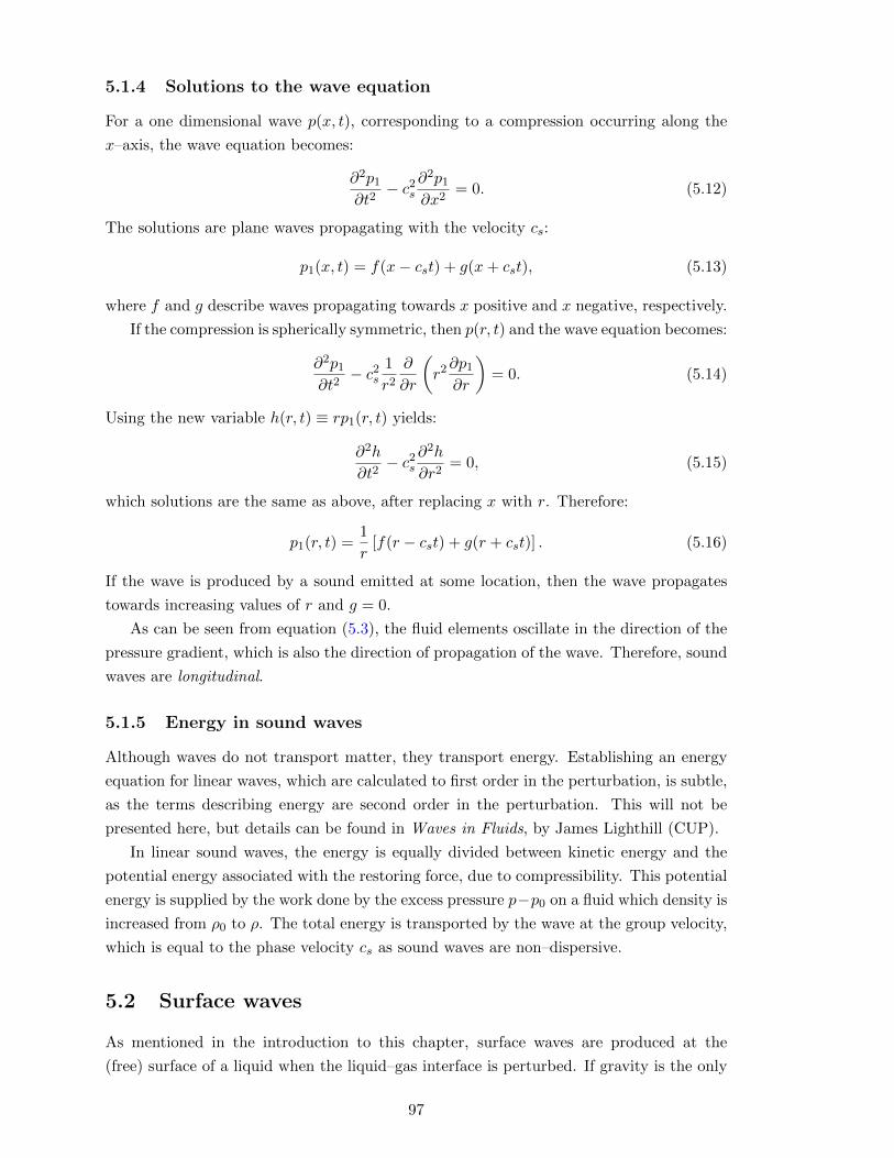
5.1.4 Solutions to the wave equation
For a one dimensional wave p(x, t), corresponding to a compression occurring along the
x–axis, the wave equation becomes:
∂2p1
∂t2− c2
s
∂2p1
∂x2= 0. (5.12)
The solutions are plane waves propagating with the velocity cs:
p1(x, t) = f(x− cst) + g(x+ cst), (5.13)
where f and g describe waves propagating towards x positive and x negative, respectively.
If the compression is spherically symmetric, then p(r, t) and the wave equation becomes:
∂2p1
∂t2− c2
s
1
r2
∂
∂r
(r2∂p1
∂r
)= 0. (5.14)
Using the new variable h(r, t) ≡ rp1(r, t) yields:
∂2h
∂t2− c2
s
∂2h
∂r2= 0, (5.15)
which solutions are the same as above, after replacing x with r. Therefore:
p1(r, t) =1
r[f(r − cst) + g(r + cst)] . (5.16)
If the wave is produced by a sound emitted at some location, then the wave propagates
towards increasing values of r and g = 0.
As can be seen from equation (5.3), the fluid elements oscillate in the direction of the
pressure gradient, which is also the direction of propagation of the wave. Therefore, sound
waves are longitudinal.
5.1.5 Energy in sound waves
Although waves do not transport matter, they transport energy. Establishing an energy
equation for linear waves, which are calculated to first order in the perturbation, is subtle,
as the terms describing energy are second order in the perturbation. This will not be
presented here, but details can be found in Waves in Fluids, by James Lighthill (CUP).
In linear sound waves, the energy is equally divided between kinetic energy and the
potential energy associated with the restoring force, due to compressibility. This potential
energy is supplied by the work done by the excess pressure p−p0 on a fluid which density is
increased from ρ0 to ρ. The total energy is transported by the wave at the group velocity,
which is equal to the phase velocity cs as sound waves are non–dispersive.
5.2 Surface waves
As mentioned in the introduction to this chapter, surface waves are produced at the
(free) surface of a liquid when the liquid–gas interface is perturbed. If gravity is the only
97

restoring force, we obtain gravity waves. At short wavelengths however, the surface tension
is important and the waves become gravity–capillary waves. We start this section by a
general analysis of surface waves, and then consider in turn these different types of waves.
The velocity and pressure satisfy Euler equation (2.30) with both pressure and gravi-
tational forces included:
ρ
(∂v
∂t+ (v ·∇) v
)= −∇p− ρgz, (5.17)
where g > 0. Surface tension forces only act at the free surface, and therefore only enter
the boundary conditions.
5.2.1 Equilibrium state
We consider an interface between water and air which is flat when at equilibrium. Water
can be approximated to be incompressible, and here we take its density ρ = ρ0 to be
constant. Viscosity is also negligible, and we assume that the flow is irrotational. This
is the case, for example, if the fluid is at rest initially (at equilibrium) as, according to
Kelvin’s theorem, a flow with constant density and subject to conservative forces retains
its vorticity at all times.
In the equilibrium state, v0 = 0, so that Euler equation (5.17) in the z–direction gives
∂p0/∂z = −ρ0g, where p0 is the pressure at equilibrium. Since the surface is flat, there
are no surface tension forces acting along its normal. Therefore, continuity of the stress
at the surface (see section 2.3.3) implies p0(z = 0) = patm, where patm is the gas pressure
at the interface. The solution of Euler equation is then:
p0(z) = −ρ0gz + patm. (5.18)
5.2.2 Boundary conditions
We consider two dimensional waves. The axis
z = 0 corresponds to the flat surface at equi-
librium and the equation of the perturbed free
surface is z = η(x, t). The depth of water is h.
The boundary conditions are as follows:
• the velocity at z = −h satisfies the no–penetration condition vz = 0,
• the velocity at the surface satisfies the kinematic boundary condition (2.38):
vz (x, η, t) =dz
dt=∂η
∂t+ vx
∂η
∂x, (5.19)
98

• as seen in section 2.3.3, when both the fluid and the gas are inviscid, continuity of
the stress implies that, at the free surface, the net pressure force is equal and opposite
to the component of the surface tension force normal to the surface.
We now calculate explicitly this latter boundary condition.
We consider a line of length L at the surface
of the water. The molecules on one side of
this line exert a pulling force (tension) on the
molecules on the other side.
This force F is tangent to the surface and perpendicular to the line. Its value per unit
length is the surface tension γ.
We now consider the forces exerted on the
dashed surface element which is between x and
x+ dx and for which the length L is along the
y–axis.
Tension forces give a resultant force dF =
F(x+ dx)−F(x) which component normal to
the surface element has to be balanced by pres-
sure forces, as seen in section 2.3.3.
In the figure above, the amplitude of the wave has been exaggerated for clarity but, in the
linear regime, this amplitude is small, so that the normal n to the surface element is equal
to z to first order. Therefore, the component of the tension force normal to the surface
element can be approximated by dFz = F(x+ dx) · z− F(x) · z. Since F(x) is tangent to
the curve η(x), the angle between F(x) and the x–axis is θ such that tan θ = ∂η/∂x. This
angle is small, so that tan θ ' sin θ ' θ, and F(x) · z = F (x) (∂η/∂x). Doing a similar
calculation for the force at x+ dx, and using F (x) = F (x+ dx) = γL, we obtain:
dFz = γL
[∂η
∂x
)x+dx
− ∂η
∂x
)x
]= γLdx
∂2η
∂x2. (5.20)
The pressure force acting on the surface element is (p(x, η, t)− patm)Ldxz. Since the
sum of the forces in the vertical direction is zero (see eq. [2.36]), we obtain the following
boundary condition:
p(x, η, t)− patm = −γ ∂2η
∂x2. (5.21)
If surface tension is negligible, that is to say γ = 0, the equation above indicates that the
pressure in the fluid is equal to the pressure in the air at the free surface.
99

5.2.3 Equation and boundary conditions for the velocity potential
Since the flow is both irrotational and incompressible, we can define a velocity potential
φ which satisfies Laplace’s equation:
∇2φ = 0. (5.22)
Instead of solving Euler and the incompressibility equations for v and p, we can solve
Laplace’s equation for φ. However, this requires to derive boundary conditions for φ from
the boundary conditions written above for v and p. This is the object of this section.
As for sound waves, we assume that the velocity and pressure in the perturbed state
can be written as v = v0 + v1(x, z, t) = v1(x, z, t) and p = p0(z) + p1(x, z, t). Then, Euler
equation (5.17) yields:
ρ0∂v1
∂t= −∇ (p0 + p1)− ρ0gz, (5.23)
where we have neglected the quadratic terms in the perturbation on the left–hand side.
Since the pressure at equilibrium satisfies −∇p0−ρ0gz = 0, the zeroth order terms cancel
out and the equation above becomes:
ρ0∂v1
∂t= −∇p1. (5.24)
Using v1 =∇φ, this equation can be written as:
∇(ρ0∂φ
∂t+ p1
)= 0, (5.25)
which gives:
p1(x, z, t) = −ρ0∂φ
∂t(x, z, t). (5.26)
Any function of time could be added to p1, but it does not need to be written explicitly as
any function of time could be added to φ anyway without changing the velocity. At the
surface z = η(x, t), the pressure p(x, η, t) ≡ p0(η) + p1(x, η, t) is given by the boundary
condition (5.21). As p0(η) is given by equation (5.18) with z = η, this yields:
p1(x, η, t) = ρ0gη(x, t)− γ ∂2η
∂x2, (5.27)
so that equation (5.26) at z = η can be written as:
∂φ
∂t(x, η, t) = −gη(x, t) +
γ
ρ0
∂2η
∂x2. (5.28)
Expanding the left–hand side in Taylor series gives:
∂φ
∂t(x, η, t) =
∂φ
∂t(x, 0, t) + η
∂2φ
∂z∂t(x, 0, t) + · · · (5.29)
Since ∇φ = v1, φ is first order in the perturbation, and the second term on the right
hand–side of the equation above is quadratic in the perturbation. To first order, we then
neglect it and substitute into equation (5.28) to obtain:
∂φ
∂t(x, 0, t) = −gη(x, t) +
γ
ρ0
∂2η
∂x2. (5.30)
100

We now use the boundary condition (5.19) which, to first order in the perturbation,
becomes:
v1,z (x, η, t) =∂η
∂t. (5.31)
(Both the displacement η and the velocity v1,x are small quantities, so v1,x(∂η/∂x) is
quadratic in the perturbation). Expanding the left–hand side in Taylor series gives:
v1,z (x, η, t) = v1,z (x, 0, t) + η∂v1,z
∂z(x, 0, t) + · · · (5.32)
Identifying with equation (5.31) and keeping only first order terms in the perturbation
then yields:
v1,z (x, 0, t) =∂η
∂t. (5.33)
Using v1,z = ∂φ/∂z, this equation can be written as:
∂φ
∂z(x, 0, t) =
∂η
∂t. (5.34)
Finally, the no–penetration condition at the bottom of the water becomes:
∂φ
∂z(x,−h, t) = 0 . (5.35)
Surface gravity waves are the solutions of Laplace’s equation (5.22) for −h ≤ z ≤ 0
subject to the boundary conditions (5.30) and (5.34) at z = 0 and (5.35) at z = −h.
5.2.4 Dispersion relation
We look for a surface displacement under the form of a sinusoidal wave travelling in the
positive x–direction, that it to say:
η(x, t) = A cos (kx− ωt) , (5.36)
where A is the amplitude of the displacement, k > 0 is the wavenumber and ω is the
frequency. Note that here we cannot think of the equilibrium state being perturbed at
some time t = 0 for example, as η cannot be zero at all values of x at a given time. The
form of η above tells us about the perturbation after it has been set up, but not about
how it was set up.
With η of the form above, equation (5.30) becomes:
∂φ
∂t(x, 0, t) = −
(g +
γk2
ρ0
)A cos (kx− ωt) , (5.37)
and equation (5.34) becomes:
∂φ
∂z(x, 0, t) = Aω sin (kx− ωt) . (5.38)
This indicates that φ is of the form:
φ(x, z, t) = f(z) sin (kx− ωt) . (5.39)
101

Substituting into Laplace’s equation (5.22), we obtain:
f ′′(z)− k2f(z) = 0.
The solutions are f(z) = C1ekz + C2e−kz, where C1 and C2 are two constants. The no–
penetration boundary condition (5.35) then yields: C1e−kh − C2ekh = 0, so that f(z) =
C cosh [k(z + h)], where C is a constant. This gives:
φ(x, z, t) = C cosh [k(z + h)] sin (kx− ωt) . (5.40)
Equation (5.37) then yields:
C =A
ω cosh(kh)
(g +
γk2
ρ0
). (5.41)
Substituting this expression for φ into equation (5.38) then gives the dispersion relation:
ω2 = gk(1 + λ2
ck2)
tanh(kh), (5.42)
where we have introduced the capillary length:
λc =
√γ
gρ0. (5.43)
It is the length below which surface tension forces dominate over gravity2. For water,
λc ' 3× 10⁻³ m at T ' 20C, and it varies only weakly with temperature.
At some time t and some position x along the x–axis, the phase of the wave is kx−ωt.At a time t+dt, this phase has advanced to x+dx such that k(x+dx)−ω(t+dt) = kx−ωt.Therefore, kdx = ωdt, and the phase velocity (speed at which the phase of the wave travels)
is given by vϕ = dx/dt = ω/k. Using the dispersion relation above, this gives:
vϕ =
√g
k(1 + λ2
ck2) tanh(kh). (5.44)
The waves are dispersive: waves with different wavenumbers travel at different speeds.
Let us assume that λc h, which is reasonable since for water λc is a few mm. We then
have the following different regimes:
• capillary waves: λ λc h,
• gravity–capillary waves on deep water: λ ' λc h,
• gravity waves on deep water: λc λ h,
• gravity waves on shallow water: λc h λ.
Since v1 = ∇φ and φ given by equation (5.40) depends both on x and z, fluid elements
oscillate in both the x and z directions so that surface waves are neither longitudinal nor
transverse.
2For example, water droplets with a radius smaller than the capillary length have a shape determined
solely by surface tension effects, and are therefore spherical.
102

5.2.5 Dispersion and group velocity
To understand the effect of dispersion, we now consider a disturbance which is the super-
position of sinusoidal waves travelling in the positive x–direction3:
η(x, t) =
ˆ +∞
0|a(k)| cos (kx− ωt) dk. (5.45)
This is the real part of:
η(x, t) =
ˆ +∞
0a(k)ei(kx−ωt)dk. (5.46)
Since ω(k), each Fourier component travels with a different speed velocity.
We assume that the coefficients a(k) are
non zero only in a narrow interval of
wavenumbers centered on k0. Such a dis-
turbance is called a wave packet and is
represented on the figure.
Performing a Taylor expansion of ω in the vicinity of k0 to first order yields:
ω(k) = ω0 + (k − k0)vg(k0), (5.47)
where we have defined:
vg =dω
dk. (5.48)
Therefore, equation (5.46) becomes:
η(x, t) = A(x, t)ei(k0x−ω(k0)t), (5.49)
with:
A(x, t) =
ˆ +∞
0a(k)ei(k−k0)(x−vg(k0)t)dk, (5.50)
where we have kept the integral from 0 to +∞, even though the Taylor expansion above is
valid only in the vicinity of k0, because the values of k outside of a narrow band centered
on k0 correspond to negligible a(k) and therefore do not contribute to the integral. This
expression shows that η can be approximated by a sinusoidal wave with wavenumber
k0 and frequency ω(k0), travelling at the speed vϕ = ω(k0)/k0, which amplitude A is a
function of x and t through the combination x− vg(k0)t.
3According to the Fourier integral theorem, any function f(x) which is absolutely integrable can be
written as:
f(x) =1√2π
ˆ +∞
−∞f(k)eikxdk,
with
f(k) =1√2π
ˆ +∞
−∞f(x)e−ikxdx.
The function f is the Fourier transform of f , and f is the inverse Fourier transform to f .
103
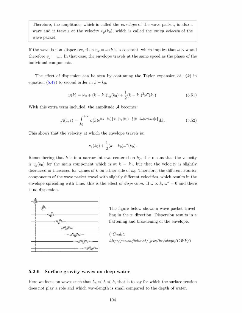
Therefore, the amplitude, which is called the envelope of the wave packet, is also a
wave and it travels at the velocity vg(k0), which is called the group velocity of the
wave packet.
If the wave is non–dispersive, then vϕ = ω/k is a constant, which implies that ω ∝ k and
therefore vg = vϕ. In that case, the envelope travels at the same speed as the phase of the
individual components.
The effect of dispersion can be seen by continuing the Taylor expansion of ω(k) in
equation (5.47) to second order in k − k0:
ω(k) = ω0 + (k − k0)vg(k0) +1
2(k − k0)2ω′′(k0). (5.51)
With this extra term included, the amplitude A becomes:
A(x, t) =
ˆ +∞
0a(k)ei(k−k0)x−[vg(k0)+ 1
2(k−k0)ω′′(k0)]tdk. (5.52)
This shows that the velocity at which the envelope travels is:
vg(k0) +1
2(k − k0)ω′′(k0).
Remembering that k is in a narrow interval centered on k0, this means that the velocity
is vg(k0) for the main component which is at k = k0, but that the velocity is slightly
decreased or increased for values of k on either side of k0. Therefore, the different Fourier
components of the wave packet travel with slightly different velocities, which results in the
envelope spreading with time: this is the effect of dispersion. If ω ∝ k, ω′′ = 0 and there
is no dispersion.
The figure below shows a wave packet travel-
ling in the x–direction. Dispersion results in a
flattening and broadening of the envelope.
( Credit:
http://www.jick.net/ jess/hr/skept/GWP/)
5.2.6 Surface gravity waves on deep water
Here we focus on waves such that λc λ h, that is to say for which the surface tension
does not play a role and which wavelength is small compared to the depth of water.
104

Phase and group velocities:
When kh 1, tanh(kh) ' 1. Therefore, the dispersion relation (5.42) can be approxi-
mated by:
ω2 = gk. (5.53)
This yields the phase velocity:
vϕ =
√g
k=
√gλ
2π. (5.54)
This shows that longer wavelengths travel faster than shorter wavelengths. The difference
between the speeds of different wavelengths is significant, as√g/(2π) = 1.25 m1/2 s−1.
Surface gravity waves in the oceans have wavelength typically in the range 1–100 m, for
which the phase velocity varies from 1.25 to 12.5 m s−1. The corresponding periods are
T = λ/vϕ in the range 0.8 to 8 s.
Differentiating the dispersion relation above yields 2ωdω = gdk, and therefore the
group velocity (5.48) is vg = dω/dk = g/(2ω), which can also be written as:
vg =1
2
√g
k=vϕ2. (5.55)
As with sound waves, the energy in linear gravity waves is equally divided between
kinetic energy and the potential energy associated with the restoring force, which here is
the gravitational potential energy, and is transported at the group velocity.
Motion of fluid elements:
The velocity potential φ is given by equations (5.40), in which C is given by equa-
tion (5.41) with the surface tension term being negligible. Since kh 1, we have
cosh(kh) ' sinh(kh) ' ekh/2, so that:
cosh [k(z + h)]
cosh(kh)=
cosh(kz) cosh(kh) + sinh(kz) sinh(kh)
cosh(kh)' ekz.
Therefore:
φ(x, z, t) =Ag
ωekz sin (kx− ωt) . (5.56)
The components of the velocity v1 =∇φ are then given by:
v1,x(x, z, t) = Aωekz cos (kx− ωt) , v1,z(x, z, t) = Aωekz sin (kx− ωt) , (5.57)
where we have used gk = ω2. We consider a fluid element which at equilibrium is at
(x0, z0). It is displaced by the perturbation so that its location becomes (x = x0 + x1, z =
z0 + z1), where |x1| and |z1| are small. We perform a Taylor expansion for v1,x:
v1,x(x, z, t) = v1,x(x0, z0, t) + x1∂v1,x
∂x(x0, z0, t) + z1
∂v1,x
∂z(x0, z0, t) + · · ·
105

Therefore, to first order in the perturbation, v1,x(x, z, t) = v1,x(x0, z0, t), and similarly for
v1,z. The velocities then only depend on time, and we can replace x by x0 and z by z0 in
equations (5.57) to obtain:
v1,x(t) = Aωekz0 cos (kx0 − ωt) , v1,z(t) = Aωekz0 sin (kx0 − ωt) . (5.58)
As v1,x = dx1/dt and v1,z = dz1/dt, we then obtain:
x1(t) = −Aekz0 sin (kx0 − ωt) +D1, z1(t) = Aekz0 cos (kx0 − ωt) +D2, (5.59)
where D1 and D2 are two constants. As mentioned above, given the form of η we have
assumed, the system is not at equilibrium at t = 0, and therefore we cannot use this
condition to calculate D1 and D2. However, the equations above yield:
(x1(t)−D1)2 + (z1(t)−D2)2 = A2e2kz0 , (5.60)
which indicates that the perturbed fluid elements move along a circle centered on (D1, D2).
Physically, this center has to be the equilibrium position of the fluid element, since x1 and
z1 are departure from equilibrium. Therefore, D1 = x0 and D2 = z0, and a fluid element
which is displaced from its equilibrium position (x0, z0) subsequently moves along a circle
centered on this point and with radius Aekz0.
The figure illustrates the path
of fluid elements displaced from
their equilibrium position. The
radius of the circles decreases
exponentially with depth.
(Credit:
https://www.nortekgroup.com/)
5.2.7 Surface gravity waves on water of finite depth
We now consider the case where we still have λc λ, that is to say surface tension does
not play a role, but when the wavelength is not small compared to the depth of water.
The dispersion relation (5.42) then becomes:
ω2 = gk tanh(kh), (5.61)
and the phase velocity is:
vϕ =
√g
ktanh(kh), (5.62)
so that here again the waves are dispersive.
106

The case corresponding to h λ, that is to say kh 1, is called the shallow water
regime. Using tanh(kh) ' kh then yields:
vϕ =√gh, (5.63)
which indicates that surface gravity waves on shallow water are non–dispersive. The
fact that vϕ decreases when the depth of water decreases explains the breaking of waves
on a steep beach. This happens because, as the wave approaches the beach, its velocity
decreases, and therefore so does its wavelength. The wave is then ‘squeezed’ into a nar-
rower volume, and its amplitude has to increase for mass to be conserved (this can also
be understood from the point of view of energy conservation, as potential energy has to
increase to compensate for the decrease in kinetic energy). This process is called shoaling.
When the amplitude of the wave is large enough, a crest overtakes the trough which is
directly in front of it and goes slower (as it reaches shallower depths first), which results
in the wave spilling or plunging forward: the wave breaks.
In the same way that we have shown that fluid elements displaced from their equilib-
rium position move along a circle in the case of deep–water, it could be shown that the
fluid elements move along ellipses in the case of finite depth. This is illustrated on the
figure below (from Ahmed et al., JMST, 2010, 24, 943), which shows that the ellipses
become more flattened as the depth of water decreases.
5.2.8 Gravity–capillary waves
Surface tension becomes important when λ is on the order of or smaller than the capillary
length λc. Such waves are called ripples. As λc is a few mm in water, the deep water
approximation is usually relevant, so that kh 1. Therefore, the dispersion relation (5.42)
becomes:
ω2 = gk(1 + λ2
ck2). (5.64)
When λck 1, gravity is negligible and we have capillary waves, for which the disper-
sion relation is ω2 = gλ2ck
3 = γk3/ρ0, where we have used equation (5.43) for λc. Their
phase and group velocities are vϕ =√γk/ρ and vg = 3vϕ/2, respectively, so that the en-
velope of wave packets travel faster than the phase of the individual Fourier components.
107

This figure shows the phase velo-
city vϕ as a function of wavelength
λ for the different type of surface
waves mentioned above. The phase
velocity has a minimum for λ ∼ λc.
5.3 Internal gravity waves
We now consider the waves for which the restoring force is gravity acting in a fluid in
which the density varies continuously with height. In general, the density decreases with
height, and this is what we assume here.
The flow satisfies Euler equation with both pressure and gravity included:
ρ
(∂v
∂t+ (v ·∇) v
)= −∇p− ρgz. (5.65)
We assume that the fluid is incompressible, so that we have:
∇ · v = 0. (5.66)
Using this condition, the mass conservation equation (1.22) yields:
Dρ
Dt=∂ρ
∂t+ (v ·∇) ρ = 0. (5.67)
It expresses the fact that, in an incompressible flow, fluid elements retain their density
as they move. This is a good approximation for describing internal gravity waves in the
oceans, but not in the atmosphere where, instead of retaining their mass density, fluid
elements retain their entropy as they move, as in the case of sound waves (section 5.1.1).
5.3.1 Buoyancy frequency
We consider a fluid element located at z and which moves upwards to z + δz while con-
serving its density ρ0(z), where ρ0 is the density at equilibrium. The density of the fluid
surrounding it at z + δz is smaller, being ρ0(z) + (dρ0/dz)δz. The fluid element, there-
fore, has an excess density over that of the surrounding fluid which is −(dρ0/dz)δz. This
results in an excess weight g(dρ0/dz)δz (directed downwards) per unit volume of fluid for
the element, so that the equation of motion for the fluid element can be written as:
ρ0d2(δz)
dt2= g
dρ0
dzδz. (5.68)
108

Therefore, the fluid element oscillates with the buoyancy frequency N defined as:
N2 = − g
ρ0
dρ0
dz. (5.69)
Here we have assumed that the displacement of the fluid element was purely vertical. As
we will see below, any additional horizontal component would reduce the frequency of
the oscillations, so that N is the maximum frequency for oscillations under gravity. The
analysis above is still valid if dρ0/dz > 0, but in that case N2 < 0 and, as will be discussed
in chapter 6, the displacement is then unstable: the fluid element keeps moving upwards
after it is displaced4.
5.3.2 Dispersion relation
We now solve the full equations above satisfied by the flow for a general linear perturbation.
We consider an equilibrium in which the velocity is zero. The density ρ0 and pressure p0
vary only with z, so that Euler equation gives:
dp0
dz+ ρ0(z)g = 0. (5.70)
As for surface waves, we consider two dimensional small perturbations in the (x, z) plane so
that v(x, z, t) = v1(x, z, t), p(x, z, t) = p0(z) +p1(x, z, t) and ρ(x, z, t) = ρ0(z) +ρ1(x, z, t),
with p1 p0 and ρ1 ρ0. Substituting in equations (5.65), (5.66) and (5.67) and keeping
only terms of first order in the perturbed quantities yield:
ρ0∂v1,x
∂t= −∂p1
∂x, ρ0
∂v1,z
∂t= −∂p1
∂z− ρ1g,
(5.71)
∂v1,x
∂x+∂v1,z
∂z= 0 ,
∂ρ1
∂t+ v1,z
dρ0
dz= 0.
Note that the zeroth order terms in equation (5.65) drop as they themselves satisfy Euler
equation.
4Here we have considered an incompressible fluid in which fluid elements retain their mass density as
they move. As mentioned already, this is a good approximation in the oceans, but not in the atmosphere
or in a star, where the fluid is a gas. A similar analysis can still be done by considering that fluid elements
retain their entropy as they move, for the same reason that we have assumed adiabatic perturbations in
the case of sound waves in section 5.1.1. On the other hand, pressure balance between the fluid element
and its new surrounding as it is displaced is achieved on a timescale shorter than the timescale on which
the displacement occurs (as it is given by the sound crossing time through the fluid element). Writing the
condition for stability in that context leads a similar result as that described in this section, but with the
buoyancy frequency (5.69) replaced by the so–called Brunt–Vaisala frequency N and defined as:
N2 = g
(1
γ
d ln p0dr
− d ln ρ0dr
),
where r is the local radius and g the local gravitational acceleration. When N2 < 0, the equilibrium is
unstable and convective motions persist. The Sun, for example, has a large convective envelope in its outer
parts in which the flow rises from below as described here.
109

We look for plane wave solutions of the form:
v1,x(x, z, t) = Vx ei(kxx+kzz−ωt), (5.72)
v1,z(x, z, t) = Vz ei(kxx+kzz−ωt), (5.73)
p1(x, z, t) = P ei(kxx+kzz−ωt), (5.74)
ρ1(x, z, t) = R ei(kxx+kzz−ωt), (5.75)
where a tilde indicates a complex quantity. The real parts have to be taken to obtain the
physical quantities. Substituting into the linearized equations (5.71) yields:
ωρoVx − kxP = 0, (5.76)
iωρ0Vz − ikzP − gR = 0, (5.77)
kxVx + kzVz = 0, (5.78)
dρ0
dzVz − iωR = 0. (5.79)
This system has a non–trivial solution only if the determinant of the coefficient matrix is
zero, which yields the dispersion relation:
ω =Nkxk
= N sin θ, (5.80)
where k =√k2x + k2
z and θ is the angle between the wavenumber k = kxx + kzz and
the z–axis. If there is no stratification, N = 0 and ω = 0, which makes it clear that
the restoring force is due to stratification. If kz = 0, ω = N , as expected since in that
case equation (5.78) implies that vx = 0 and the fluid elements oscillate as described in
section 5.3.1. If kx = 0, ω = 0, again as expected since in that case equation (5.78)
implies that vz = 0, which means that the motion is in the x–direction in which there
is no restoring force. For that reason as well, the frequency of the oscillations is smaller
when the motion is not purely vertical, so that ω ≤ N .
Here we have considered a free oscillation, that is to say an oscillation that results from
some initial disturbance and occurs with the system own natural frequency. If instead the
oscillation were forced, then both k and ω would be given by the forcing process. For
example, when the waves are produced by water flowing over a ridge in the ocean or air
moving over hills in the atmosphere, k is given by the geometry of the ridge/hills and ω
by the speed of the flow. The result above then shows that only waves with frequencies
smaller than N can propagate.
The phase velocity is vϕ = ω/k and is in the direction of k, so that we can write:
vϕ =Nkxk2
k
k. (5.81)
In the same way that we have shown that the group velocity for a one dimensional wave
is vg = dω/dk (section 5.2.5), we could show that, in two dimensions:
vg =∂ω
∂kxx +
∂ω
∂kzz. (5.82)
110

Therefore, here, we obtain:
vg =Nkzk3
(kzx− kxz) . (5.83)
This shows that the group velocity is perpendicular to the direction in which the wave
propagates!
In other words, the envelope of wave packets and the
energy propagate in a direction which is perpendicu-
lar to the direction of propagation of the crests and
troughs, as illustrated on the figure.
(Credit: http://www.po.gso.uri.edu )
5.3.3 Motion of fluid elements
Equation (5.78) can also be written as k · v1 = 0, which means that the waves are trans-
verse: fluid elements oscillate along lines perpendicular to the direction of propagation k,
that is to say along lines of constant phase.
The figure illustrates the motion of a fluid ele-
ment (represented by the blue dot). The pres-
sure force Fp = −∇p = −kp is perpendicular
to the lines of constant phase and directed up-
wards (since pressure decreases upwards). The
weight W is downwards, and the resultant net
force is along the line of constant phase, as this
is the line along which the fluid element moves.
We can recover the frequency of the oscillations by doing the same analysis as in sec-
tion 5.3.1. A displacement δl along a line of constant phase corresponds to a vertical
displacement δz = δl sin θ. Therefore, the weight W acting on the excess mass that
the fluid element has relative to its surrounding is W = −N2δz = −N2δl sin θ per unit
mass of the fluid element. The component of the weight perpendicular to the line of
constant phase balances the pressure force, so the net force acting on the fluid element
is W sin θ = −N2δl sin2 θ. Therefore, writing an equation of motion similar to equa-
tion (5.68) (replacing δz by δl), we obtain that the frequency of the oscillations is N sin θ,
in agreement with equation (5.80).
111

The figure illustrates the motion of fluid
elements and propagating internal grav-
ity waves.
(Credit: http://www-eaps.mit.edu )
112

Chapter 6
Instabilities and turbulence
In chapter 5, we have discussed the propagation of small perturbations in a fluid. As
already mentioned, using the Fourier integral theorem, it is always possible to write a
perturbation as a linear combination of Fourier components ei(kx−ωt), the physical quantity
being the real part of this complex function. We obtain a relation between ω and k
(dispersion relation) by writing that the perturbed quantities satisfy Euler’s equation,
the incompressibility condition and the boundary conditions. For surface waves, we have
found that ω was always real, which means that the perturbation is a wave propagating
in the positive x direction. However, in the case of internal gravity waves, when N2 given
by equation (5.69) is negative, which is the case when the mass density increases with
height, the dispersion relation (5.80) yields the imaginary frequency ω = ±i√−N2kx/k.
The term e|ω|t is then present in the expression of the perturbation, which means that
the perturbation grows with time: it is unstable. This is not surprising as a heavy fluid
element displaced downwards, where the fluid is lighter, will continue to sink instead of
oscillating around its equilibrium position.
Linear stability theory deals with the growth of very small perturbations which can be
treated in the same way as we have treated waves in the previous chapter, by keeping only
first order terms in the perturbation in the equations. Of course, after the perturbations
grow beyond some amplitude, linear theory is not valid anymore. Therefore, this theory
only allows to study the onset of instabilities, and cannot be used to describe the develop-
ment of the instability when non–linear terms become important. As we are going to see
in this chapter, there are a number of instabilities which develop starting with very small
perturbations. However, in some cases, instabilities arise only when perturbations reach
a certain amplitude. These are called finite amplitude instabilities and will not be studied
here.
6.1 Kelvin–Helmholtz instability
We consider a fluid of density ρ2 which is above another fluid or density ρ1 > ρ2. Both
fluids are inviscid and incompressible, and we take their densities to be constant. When the
interface between them is perturbed, we obtain stable surface gravity waves, as studied
113

in chapter 5. However, the perturbation may become unstable if the two fluids move
with respect to each other. In other words, a gravitationally stable stratification may be
destabilized by shear. This is called a Kelvin–Helmholtz instability and is the focus of this
section.
We assume that the fluid on top moves with velocity U x, where U is a constant,
whereas the fluid at the bottom is at rest. At equilibrium, the interface between the two
fluids is flat and in the z = 0 plane.
The interface between the two fluids is
perturbed such that its equation becomes
z = η(x, t), with η being the real part of:
η(x, t) = Aei(kx−ωt). (6.1)
6.1.1 Boundary conditions
The analysis presented here follows closely that done for surface waves in section 5.2. We
take into account gravitational, pressure and surface tension forces. Both fluids satisfy
Euler equation (2.30):
ρ
(∂v
∂t+ (v ·∇) v
)= −∇p− ρgz, (6.2)
where g > 0.
The boundary conditions at the interface are as follows:
• the kinematic condition (2.34) yields:
vi,z =dz
dt=∂η
∂t+ vi,x
∂η
∂x, (6.3)
where vi,x and vi,z are the components of the velocity in fluid i, for i = 1, 2;
• pressure forces are equal and opposite to surface tension forces (see section 2.3.3).
As shown in chapter 5, this yields (see eq. [5.21]):
p1(x, η, t)− p2(x, η, t) = −γ ∂2η
∂x2, (6.4)
where p1 and p2 are the pressures in fluids 1 and 2, respectively, and γ is the surface
tension.
6.1.2 Dispersion relation
We note vi = vi,0 + v′i the velocity in fluid i, where vi,0 is the velocity at equilibrium
and v′i is the perturbed velocity. We have v2,0 = U x and v1,0 = 0. Since the fluids are
114

incompressible, we can then define the velocity potential φi such that vi = ∇φi. Given
that the fluids at equilibrium are also incompressible, we can write φi = φi,0 + φ′i, with
vi,0 =∇φi,0 and v′i =∇φ′i. Similarly, we have pi = pi,0 + p′i, where pi,0 is the pressure at
equilibrium and p′i is the perturbed pressure in fluid i.
In equation (6.3), vi,z is the perturbed velocity since the equilibrium velocity has no
vertical component. Therefore, this equation gives:
∂φ′1∂z
(x, η, t) =∂η
∂t, (6.5)
∂φ′2∂z
(x, η, t) =∂η
∂t+ U
∂η
∂x, (6.6)
to first order in the perturbation. To this order, we also have that ∂φ′i/∂z at (x, η, t) is
equal to its value at (x, 0, t) (see section 5.2.3). Therefore, we obtain:
∂φ′1∂z
(x, 0, t) =∂η
∂t,
∂φ′2∂z
(x, 0, t) =∂η
∂t+ U
∂η
∂x.
(6.7)
(6.8)
Since the flows are irrotational and with constant densities, Bernoulli’s theorem can
be expressed as (eq. [2.59]):
ρi∂φi∂t
+1
2ρiv
2i + pi + ρigz = 0, (6.9)
which can be written as:
ρi∂
∂t
(φi,0 + φ′i
)+
1
2ρi
[(vi,0 + v′i,x
)2+ v′2i,z
]+ pi + ρigz = 0. (6.10)
For fluid 1, this gives at z = η:
ρ1∂φ′1∂t
(x, η, t) + p1 (x, η, t) + ρ1gη (x, t) = 0, (6.11)
where we have neglected v′21,z and v′21,x, as they are second order in the perturbation. To
first order, ∂φ′1/∂t at (x, η, t) is equal to its value at (x, 0, t) (see section 5.2.3). Therefore,
equation (6.11) yields:
p1(x, η, t) = −ρ1
(∂φ′1∂t
(x, 0, t) + gη (x, t)
). (6.12)
For fluid 2, equation (6.10) at z = η becomes:
ρ2∂φ′2∂t
(x, η, t) +1
2ρ2U
2 + ρ2U∂φ′2∂x
(x, η, t) + p2 (x, η, t) + ρ2gη (x, t) = 0, (6.13)
where we have used v′2,x = ∂φ′2/∂x and neglected second order terms. Since any function
of time can be added to φ′2 without changing the velocities, the term ρ2U2/2 can be
subsumed into ∂φ′2/∂t by adding U2t/2 to φ′2. Replacing ∂φ′2/∂t and ∂φ′2/∂x at (x, η, t)by
their values at (x, 0, t) then yields:
p2(x, η, t) = −ρ2
(∂φ′2∂t
(x, 0, t) + U∂φ′2∂x
(x, 0, t) + gη (x, t)
). (6.14)
115

Substituting equations (6.12) and (6.14) into the boundary condition (6.4) then gives:
ρ1
(∂φ′1∂t
(x, 0, t) + gη
)− ρ2
(∂φ′2∂t
(x, 0, t) + U∂φ′2∂x
(x, 0, t) + gη
)= γ
∂2η
∂x2. (6.15)
As in the case of surface waves (section 5.2.4), we look for complex solutions under the
form:
φ′1 = f1(z)ei(kx−ωt), φ′2 = f2(z)ei(kx−ωt). (6.16)
Since both φ′1 and φ′2 satisfy Laplace’s equation, we have:
f ′′i(z)− k2fi(z) = 0.
The solutions are a linear combination of ekz and e−kz. We assume that the height of fluid
on both sides of the interface is large compared to the wavelength of the perturbation, so
that φ′1 and φ′2 go to zero when z go to −∞ and +∞, respectively. This implies f1 = K1ekz
and f2 = K2e−kz, where K1 and K2 are two constants.
Inserting in equations (6.7), (6.8) and (6.15) then yields:
K1k = −iωA,
−K2k = iωA(−ω + Uk),
ρ1 (−iωK1 + gA)− ρ2 (−iωK2 + iUK2k + gA) = −γk2A.
This system has a non–trivial solution for K1, K2 and A only if the following dispersion
relation is satisfied:
(ρ1 + ρ2)ω = ρ2Uk ±
(ρ1 + ρ2)[γk3 + (ρ1 − ρ2) gk
]− ρ1ρ2U
2k21/2
. (6.17)
6.1.3 Instability condition
If the term in the square root in equation (6.17) is negative, then ω is complex and can
be written as ω = ωR± iωI . In that case, the term e|ωI |t is present in the expression of φ′1
and φ′2 given by equation (6.16): the perturbation grows exponentially with time, which
means it is unstable1.
Therefore, the instability condition is:
(ρ1 + ρ2)[γk3 + (ρ1 − ρ2) gk
]− ρ1ρ2U
2k2 < 0, (6.18)
1Any general disturbance can be written as:
ˆ +∞
−∞a(k)ei(kx−ω(k)t)dk.
Therefore, if there exists a value of k for which ω(k) is complex, the perturbation will grow exponentially
with time. Instability can only be avoided if a(k) = 0 for the unstable wavenumbers, which requires the
perturbation to select particular values of k.
116

which can also be written as:
ρ1ρ2U2
(ρ1 + ρ2)2 > c20, (6.19)
where we have defined:
c20 =
ρ1 − ρ2
ρ1 + ρ2
g
k
(1 +
γk2
g (ρ1 − ρ2)
). (6.20)
c0 is the phase velocity of the surface wave which propagates as a result of the perturbation
when U = 0 (when ρ2 ρ1, we recover ω/k with ω given by eq. [5.64]).
The figure shows the region of instability
in the (k, U) plane.
The minimum velocity c0,min is given by:
c0,min =2
ρ1 + ρ2
√γg (ρ1 − ρ2), (6.21)
and it corresponds to the wavenumber kc = 1/λc, where λc is the capillary length:
λc =
√γ
g (ρ1 − ρ2). (6.22)
This is equivalent to equation (5.43) when ρ2 ρ1.
6.1.4 Physics of the instability
When the interface is perturbed, the
streamlines are brought closer to each
other above the crests and below the
troughs, so that the flow velocity in-
creases there (due to mass conservation),
which implies that the pressure decreases
(due to Bernoulli’s theorem).
117

Similarly, the velocity decreases and the pressure increases under the crests and above the
troughs. Therefore, pressure forces amplify the perturbation, which is the basis of the
instability. Gravitational forces tend to stabilize the flow, as they oppose the upwards
motion of the heavier fluid which is at the bottom. Similarly, surface tension stabilizes
the flow by opposing the deformation of the interface. Gravitation and capillarity are
more effective at large and small wavelengths, respectively, with comparable contribution
at λ ∼ λc.
When the perturbation starts growing, the upper part of the interface moves with the
velocity of the fluid at the top whereas the lower part moves with the velocity of the fluid
at the bottom, which results in the deformation of the fronts and produces a rolling up of
the interface, as indicated on the figure below:
The evolution of the flow can also be understood in terms of the vorticity. At equilibrium,
the circulation´C v ·dl around a rectangular contour C across the interface with two sides
parallel to the interface is equal to ±UL, where L is the length of the sides along the
x–axis. Using Stokes theorem, this is equal to the flux of vorticity through the surface
delimited by the contour. Since the flows on both sides are irrotational at equilibrium, the
vorticity is localized on the interface, where the shear is present (as U varies discontinu-
ously at the interface). When the interface is perturbed, this vorticity sheet is deformed,
and the subsequent evolution is constrained by Kelvin’s theorem.
This instability may also occur when
there is a continuous gradient of density
and velocity, instead of a sudden jump at
an interface, as in layers of clouds.
6.2 Rayleigh–Taylor instability
See Problem Set 5.
118

6.3 Turbulence
In some cases, the growth of perturbations due to instabilities in the non–linear regime
leads to a transition to turbulence. The instabilities described in the above sections are
due to a particular gradient of density or velocity. However, it is an experimental fact
that every shear flow becomes turbulent when its Reynolds number exceeds a critical
value Rec ∼ 103. The structure of a turbulent flow is very complex and non predictable.
However, statistical methods can be used to derive some properties of turbulence. In this
section, we assume that the density ρ is constant (in space and time), which implies that
the fluid is incompressible.
6.3.1 The Reynolds stress
In a turbulent flow, velocities have random fluctuations around a mean value. This is
expressed by the co–called Reynolds decomposition:
v = V + v′, (6.23)
where V = 〈v〉 and 〈v′〉 = 0, with the brackets denoting an average. The different
quantities depend both on location r and on time t. In general, if the flow is time–
dependent, 〈v〉 corresponds to the average of the velocity over a large ensemble of flows
with the same properties. However, if the flow varies on a timescale T long compared
to the characteristic timescale τ of the fluctuations, or if the flow is time–independent
(infinite T ), the average may be calculated over a time large compared to τ and small
compared to T . A similar decomposition can be made for the pressure and the viscous
stress tensor (2.13):
p = P + p′, σij = Sij + σ′ij , (6.24)
where P = 〈p〉, Sij = 〈σij〉 and 〈p′〉 =⟨σ′ij
⟩= 0. Given the way average quantities are
calculated, it is straightforward to show that the spatial derivative of an average quantity
is equal to the average of the spatial derivative of that quantity:
∂ 〈〉∂xi
=
⟨∂
∂xi
⟩.
This is also valid for the time–derivative:
∂ 〈〉∂t
=
⟨∂
∂t
⟩,
but, when the flow is time–dependent, this requires τ T .
Interchanging the average and space derivatives, we can write the average of the viscous
stress as:
Sij = ρν
(∂Vi∂xj
+∂Vj∂xi
). (6.25)
The flow satisfies Navier–Stokes equation (2.20):
ρ∂vi∂t
+ ρ (v ·∇) vi = − ∂p
∂xi+∂σij∂xj
+ fi, (6.26)
119

where f includes all the forces per unit volume which act on the fluid. Using the Reynolds
decomposition above, this equation can be re–written as:
ρ∂
∂t
(Vi + v′i
)+ ρ
[(V + v′
)·∇] (Vi + v′i
)= − ∂
∂xi
(P + p′
)+
∂
∂xj
(Sij + σ′ij
)+ fi. (6.27)
We now average this equation over a time long compared to τ but small compared to T .
Using the fact that the time and space derivatives can be interchanged with the averages,
and that the average of the fluctuations is zero, this yields:
ρ∂Vi∂t
+ ρ (V ·∇)Vi + ρ⟨(
v′ ·∇)v′i⟩
= − ∂P∂xi
+∂Sij∂xj
+ fi. (6.28)
We have assumed that the flow is incompressible, that is to say:
∇ ·(V + v′
)= 0. (6.29)
Taking a time–average of this equation yields:
∇ ·V = 0, (6.30)
which means that the average flow is incompressible. Subtracting from equation (6.29)
then gives:
∇ · v′ = 0, (6.31)
which means that the fluctuations are also incompressible. Therefore, the term ρ (V ·∇)Vi
in equation (6.28) can be written as:
ρVj∂Vi∂xj
=∂
∂xj(ρVjVi) ,
where we have used the incompressibility of the average velocity. Similarly, the term
ρ 〈(v′ ·∇) v′i〉 in equation (6.28) can be written as:
ρ
⟨v′j∂v′i∂xj
⟩=
⟨∂
∂xj
(ρv′jv
′i
)⟩=
∂
∂xj
⟨ρv′jv
′i
⟩,
where we have used the incompressibility of the fluctuations and interchanged the space
derivatives and average. Therefore, equation (6.28) becomes:
ρ∂Vi∂t
+∂
∂xj
(ρVjVi + ρ
⟨v′jv′i
⟩)= − ∂P
∂xi+∂Sij∂xj
+ fi, (6.32)
which can also be written in the form:
ρ∂Vi∂t
+∂
∂xj
(ρVjVi + ρ
⟨v′jv′i
⟩+ Pδij − Sij
)= fi. (6.33)
This equation expresses the fact that the rate of change of momentum in a fixed volume
(∂/∂t term) is due to the divergence of the momentum flux (∂/∂xj term) and to the forces
acting on the volume. This is similar to equation (2.19), but with the addition of the
Reynolds stress, also called turbulent stress:
τij = −ρ⟨v′jv′i
⟩. (6.34)
Therefore, in a turbulent flow, momentum is transported by the mean velocities, by viscos-
ity and pressure, as in a laminar flow, but also by the correlations between the components
of the fluctuations.
120

6.3.2 Mixing length theory
As we have no expression for the components of τij (six of which are independent, as the
tensor is symmetrical), the problem has more unknowns than equations. This is the well–
known closure problem of turbulence. Since τij appears in the same way as Sij = 〈σij〉in equation (6.33), it is tempting to express τij by analogy with 〈σij〉, which is given by
equation (6.25). This is the basis for the mixing length theory, in which τij is written as:
τij = ρνt
(∂Vi∂xj
+∂Vj∂xi
). (6.35)
where νT is the so–called turbulent, or eddy viscosity. By analogy with expression (2.5)
for the molecular viscosity, it is supposed that:
νT ∼ vTΛ, (6.36)
where vt is a characteristic velocity of the turbulent eddies and Λ is the so–called mixing
length, which is the “mean free path” of the eddies, i.e. the distance they travel through
before they mix with their environment. Both vt and Λ depend on the flow under consid-
eration. Mixing length theory is widely used, for example to model the convective zone
of stars. However, although in this context it describes well the transport of energy by
the turbulent flow, it fails to give an accurate description of the transport of momentum.
This is a problem when modelling the interaction between the convective flow and tidal
oscillations excited by a stellar companion in binary systems, for example. One of the
limitation of the model is that the scale of the largest turbulent eddies is comparable to
the scale on which the average quantities vary. This is in constrast to kinetic theory, where
the calculation of the viscosity relies on the separation between the scale on which random
motions occur and the scale over which quantities are averaged.
6.3.3 Energy conservation
The kinetic energy per unit mass is:
1
2v2i =
1
2
(Vi + v′i
)2=
1
2
(V 2i + v′2i + 2Viv
′i
).
Therefore, the average kinetic energy per unit mass is:
1
2
(V 2i +
⟨v′2i⟩),
which is the sum of the kinetic energy of the mean flow and that of the fluctuations.
We obtain an energy conservation equation for the mean flow by multiplying equa-
tion (6.28) by Vi:
∂
∂t
(1
2V 2i
)+ ViVj
∂Vi∂xj
+ Vi
⟨v′j∂v′i∂xj
⟩= −Vi
ρ
∂P
∂xi+ νVi
∂
∂xj
(∂Vi∂xj
+∂Vj∂xi
), (6.37)
121

where we have neglected gravity, and where summation over i and j is implicit. Using the
incompressibility of the average velocity (eq. [6.30]), we have:
Viρ
∂P
∂xi=
∂
∂xi
(ViP
ρ
),
and:
Vi∂
∂xj
(∂Vi∂xj
+∂Vj∂xi
)= Vi
∂2Vi∂x2
j
=∂
∂xj
(Vi∂Vi∂xj
)−(∂Vi∂xj
)2
.
Using the incompressibility of the fluctuations (eq. [6.31]) yields:
Vi
⟨v′j∂v′i∂xj
⟩= Vi
⟨∂
∂xj
(v′jv′i
)⟩.
Interchanging the average and space derivatives, this can be written as:
Vi∂
∂xj
⟨v′jv′i
⟩=
∂
∂xj
(Vi⟨v′jv′i
⟩)−⟨v′jv′i
⟩ ∂Vi∂xj
.
Therefore, equation (6.37) becomes:
∂
∂t
(V 2i
2
)+Vj
∂
∂xj
(V 2i
2
)=
∂
∂xj
(−VjP
ρ+ νVi
∂Vi∂xj− Vi
⟨v′jv′i
⟩)− ν
(∂Vi∂xj
)2
+⟨v′jv′i
⟩ ∂Vi∂xj
. (6.38)
This equation expresses the conservation of kinetic energy for the mean flow. It indicates
that the Lagrangian derivative of V 2i /2 (left hand–side) is equal to the divergence of a
flux, which represents the work done by pressure forces, viscous and Reynolds stresses,
plus a term expressing dissipation of energy in the mean flow due to viscosity, which
is ν (∂Vi/∂xj)2, plus a term which represents the transport of mean momentum by the
Reynolds stress, which is⟨v′jv′i
⟩(∂Vi/∂xj).
A similar conservation equation for the fluctuations can be obtained by multiplying
equation (6.26) by v′i:
v′i∂vi∂t
+ v′ivj∂vi∂xj
= −v′i
ρ
∂p
∂xi+ νv′i
∂
∂xj
(∂vi∂xj
+∂vj∂xi
). (6.39)
Using the Reynolds decomposition and averaging over time yields:
∂
∂t
(v′2i2
)+
⟨v′iVj
∂v′i∂xj
⟩+
⟨v′iv′j
∂v′i∂xj
⟩+
⟨v′iv′j
∂Vi∂xj
⟩=
−⟨v′iρ
∂p′
∂xi
⟩+ ν
⟨v′i
∂
∂xj
(∂v′i∂xj
+∂v′j∂xi
)⟩. (6.40)
As above, we use the incompressibility of the average and fluctuating velocities to re–write
this equation as:
∂
∂t
(⟨v′2i⟩
2
)+ Vj
∂
∂xj
(⟨v′2i⟩
2
)=
∂
∂xj
−⟨v′jp′⟩
ρ+ ν
⟨v′i∂v′i∂xj
⟩−
⟨v′jv′2i
⟩2
− ν⟨( ∂v′i∂xj
)2⟩−⟨v′jv′i
⟩ ∂Vi∂xj
. (6.41)
122

Here again, this equation expresses the conservation of kinetic energy for the fluctua-
tions. It indicates that the Lagrangian derivative of⟨v′2i⟩/2 (left hand–side) is equal to
the divergence of a flux, which represents the average of the work done by the fluctuat-
ing pressure forces, viscous and Reynolds stresses, plus a term expressing dissipation of
energy in the fluctuations due to viscosity, which is ν⟨
(∂v′i/∂xj)2⟩
, plus the same term
as in equation (6.38) which represents the transport of mean momentum by the Reynolds
stress, which is −⟨v′jv′i
⟩(∂Vi/∂xj). This term has a positive sign in equation (6.38),
and a negative sign here. It means that energy is transferred from the mean flow to the
fluctuations.
6.3.4 Kolmogorov scaling
When the fluctuations are stationary and vary slowly in space, equation (6.41) gives:
⟨v′jv′i
⟩ ∂Vi∂xj
= −ν
⟨(∂v′i∂xj
)2⟩, (6.42)
which shows that the energy received by the fluctuations from the mean flow (left hand
side) is dissipated by viscosity (right hand side).
We now present the Kolmogorov model, which describes how the energy which is
fed into the fluctuations from the mean flow is ultimately dissipated by viscosity. The
turbulence can be modelled as a superposition of vortices, also called turbulent eddies,
of different sizes. The Kolmogorov model, which applies to homogeneous and isotropic
turbulence, assumes that the energy from the mean flow is fed into the largest eddies,
and that it subsequently cascades down to the smallest eddies where it is dissipated by
viscosity.
The largest eddies have a characteristic size and velocity that we note l and vl, re-
spectively. Let ε be the energy per unit mass which is transferred by the mean flow to
the largest eddies per unit time. The units of ε are J kg−1 s−1, which is equal to m2 s−3.
Dimensional analysis then yields:
ε ∼ v3l /l. (6.43)
This energy is then passed on continuously to smaller eddies. Therefore, the same argu-
ment applies to an eddy of size λ and velocity vλ receiving the energy ε per unit mass and
per unit time, so that:
ε ∼ v3λ/λ. (6.44)
When the energy reaches the smalles eddies, which have a size l0 and a velocity v0, it
is dissipated by viscosity, Therefore, ε is equal to the term on the right hand side of
equation (6.42) evaluated for the smallest eddies, which gives:
ε ∼ νv20/l
20. (6.45)
Writing equation (6.44) for vλ = v0 and λ = l0 and comparing with equation (6.45) then
yields the Komolgorov length and velocity::
l0 ∼ ν3/4ε−1/4, v0 ∼ (νε)1/4. (6.46)
123

The kinetic energy per unit mass of an eddy of size λ and velocity vλ is v2λ/2, which
according to equation (6.44) is proportional to (ελ)2/3. Therefore, larger eddies have more
energy.
The range of scales λ ∼ l is called the energy range, as this is where most of the energy
is. The scales λ ∼ l0 are called dissipation range, and the intermediate scales l0 λ l
are called the inertial range.
A very important law in the theory of turbulence is the so–called Kolmogorov’s sim-
ilarity law, which is obtained by introducing the wavenumber k such that λ ∼ 1/k. We
then note E(k)dk the kinetic energy per unit mass in the eddies with wavenumber between
k and k + dk. The quantity E(k) is the spectral energy density and is associated with
the Fourier decomposition of the turbulent velocities. In the inertial range, this energy
cannot depend on l, l0 or ν. Therefore, it can only depend on ε and on k. Since it has the
dimensions m3 s−2, dimensional analysis yields:
E(k) ∼ ε2/3k−5/3. (6.47)
Note that, for k = 1/λ:
ˆ +∞
kE(k′)dk′ ∝ ε2/3k−2/3 ∼ (ελ)2/3 ∼ v2
λ.
This means that the total energy in all the eddies with sizes smaller than λ is roughly
equal to the energy of the eddies with size λ, which is consistent with the result that the
energy is in the largest eddies.
124

Appendix A
Complex variables
A.1 The Cauchy–Riemann relations
A function is analytic in a domain if it is single–valued and differentiable at all points in
this domain. For the function w(z) to be differentiable, the limit:
L = lim∆z→0
w(z + ∆z)− w(z)
∆z,
must exist and be unique. With z = x + iy and w(z) = φ(x, y) + iψ(x, y), this limit can
also be written as:
L = lim∆x,∆y→0
φ(x+ ∆x, y + ∆y) + iψ(x+ ∆x, y + ∆y)− φ(x, y)− iψ(x, y)
∆x+ i∆y,.
This limit should not depend on the direction along which we approach the point (x, y).
Therefore, the result corresponding to ∆z being purely real (∆y = 0), which is:
L = lim∆x→0
φ(x+ ∆x, y) + iψ(x+ ∆x, y)− φ(x, y)− iψ(x, y)
∆x=∂φ
∂x+ i
∂ψ
∂x,
should be identical to the result corresponding to ∆z being purely imaginary (∆x = 0),
which is:
L = lim∆y→0
φ(x, y + ∆y) + iψ(x, y + ∆y)− φ(x, y)− iψ(x, y)
i∆y= −i
∂φ
∂y+∂ψ
∂y.
By equating the real and imaginary parts of these two expressions, we see that φ and ψ
have to satisfy the Cauchy–Riemann relations:
∂φ
∂x=∂ψ
∂y, and
∂ψ
∂x= −∂φ
∂y. (A.1)
It is straightfoward to see that these relations imply ∂2φ/∂x2 +∂2φ/∂y2 = 0, and similarly
for ψ, so that both the real and imaginary parts of an analytic function satisfy Laplace’s
equation. A function that satisfies Laplace’s equation is called a harmonic function.
The derivative of w can then be calculated by keeping y constant:
dw
dz=∂φ
∂x+ i
∂ψ
∂x. (A.2)
125

A.2 Cauchy’s theorem
A.3 Laurent series
126

![FLUIDS and ELECTROLYTES BODY FLUIDS Functions of Fluids Body fluids: Facilitate in the transport [nutrients, hormones, proteins, & others…] Aid in removal](https://img.pdfslide.net/doc/110x75/56649f225503460f94c3a044/fluids-and-electrolytes-body-fluids-functions-of-fluids-body-fluids-facilitate.jpg)