UNIVERSITY OF SIEGEN

MASTER PRAKTIKUM

Fluorescence Correlation Spectroscopy

Authors:Nemanja Markesevic, AssegidFlatae, Florian Sledz, AmrFarrag and Mario Agio

Laboratory of Nano-opticsDepartment of Physics

November 9, 2019

ii

————————————————————————————-

iii

UNIVERSITY OF SIEGEN

Faculty of Physics

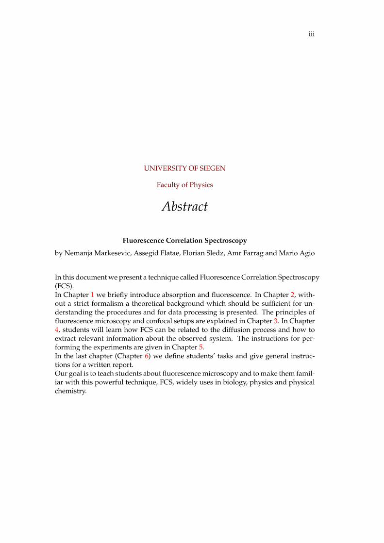
Abstract

Fluorescence Correlation Spectroscopy

by Nemanja Markesevic, Assegid Flatae, Florian Sledz, Amr Farrag and Mario Agio

In this document we present a technique called Fluorescence Correlation Spectroscopy(FCS).In Chapter 1 we briefly introduce absorption and fluorescence. In Chapter 2, with-out a strict formalism a theoretical background which should be sufficient for un-derstanding the procedures and for data processing is presented. The principles offluorescence microscopy and confocal setups are explained in Chapter 3. In Chapter4, students will learn how FCS can be related to the diffusion process and how toextract relevant information about the observed system. The instructions for per-forming the experiments are given in Chapter 5.In the last chapter (Chapter 6) we define students’ tasks and give general instruc-tions for a written report.Our goal is to teach students about fluorescence microscopy and to make them famil-iar with this powerful technique, FCS, widely uses in biology, physics and physicalchemistry.

v

Contents

Abstract iii

1 Fluorescence 11.1 Optical transitions in molecules . . . . . . . . . . . . . . . . . . . . . . . 1

1.1.1 Jablonski diagram . . . . . . . . . . . . . . . . . . . . . . . . . . 11.1.2 Fluorescence quantum yield . . . . . . . . . . . . . . . . . . . . . 21.1.3 Saturation intensity . . . . . . . . . . . . . . . . . . . . . . . . . . 21.1.4 Examples of fluorescent molecules . . . . . . . . . . . . . . . . . 3

1.2 Rhodamine 6G . . . . . . . . . . . . . . . . . . . . . . . . . . . . . . . . . 4

2 Introduction to Fluorescence Correlation Spectroscopy 72.1 Auto-correlation and Cross-correlation . . . . . . . . . . . . . . . . . . . 7

2.1.1 Auto- and Cross-correlation in Fluorescence (Cross-) correla-tion spectroscopy . . . . . . . . . . . . . . . . . . . . . . . . . . . 7

3 Experimental approach to FCS 93.1 Optical setup . . . . . . . . . . . . . . . . . . . . . . . . . . . . . . . . . . 9

3.1.1 Detectors . . . . . . . . . . . . . . . . . . . . . . . . . . . . . . . . 93.1.2 Dark counts and afterpulsing . . . . . . . . . . . . . . . . . . . . 103.1.3 Time Tagged Time-Resolved (TTTR) data collection . . . . . . . 103.1.4 Confocal setup . . . . . . . . . . . . . . . . . . . . . . . . . . . . 103.1.5 Confocal volume - geometrical interpretation . . . . . . . . . . . 12

4 FCCS and Diffusion 134.1 Diffusion . . . . . . . . . . . . . . . . . . . . . . . . . . . . . . . . . . . . 13

4.1.1 Interpretation of the equations . . . . . . . . . . . . . . . . . . . 14

5 Instructions for measurements 155.1 Measurements . . . . . . . . . . . . . . . . . . . . . . . . . . . . . . . . 15

5.1.1 Samples . . . . . . . . . . . . . . . . . . . . . . . . . . . . . . . . 155.1.2 Measurements of fluorescence spectra . . . . . . . . . . . . . . . 155.1.3 Correlation curves . . . . . . . . . . . . . . . . . . . . . . . . . . 165.1.4 Saturation curve . . . . . . . . . . . . . . . . . . . . . . . . . . . 17

6 Students’ tasks 196.1 Tasks . . . . . . . . . . . . . . . . . . . . . . . . . . . . . . . . . . . . . . 196.2 Output . . . . . . . . . . . . . . . . . . . . . . . . . . . . . . . . . . . . . 19

Bibliography 21

1

Chapter 1

Fluorescence

1.1 Optical transitions in molecules

Spectroscopy probes the properties of matter using the interaction between electro-magnetic waves and matter. This includes molecules, which are quantum mechani-cal systems with discrete energy levels (vibrational, rotational and electronic).Molecules can, for example, absorb ultraviolet or visible light undergoing a transi-tion to a higher electronic energy level. Likewise, the absorbed energy can be lostthrough the emission of a photon. This process can be fast (of the order of 1 ns),when the transition does not involve a change in the electronic spin, and it is calledfluorescence. On the other hand, phosphorescence can be a very slow process (up toseconds), because the associated transition requires a change in the electronic spin,which is in principle forbidden.

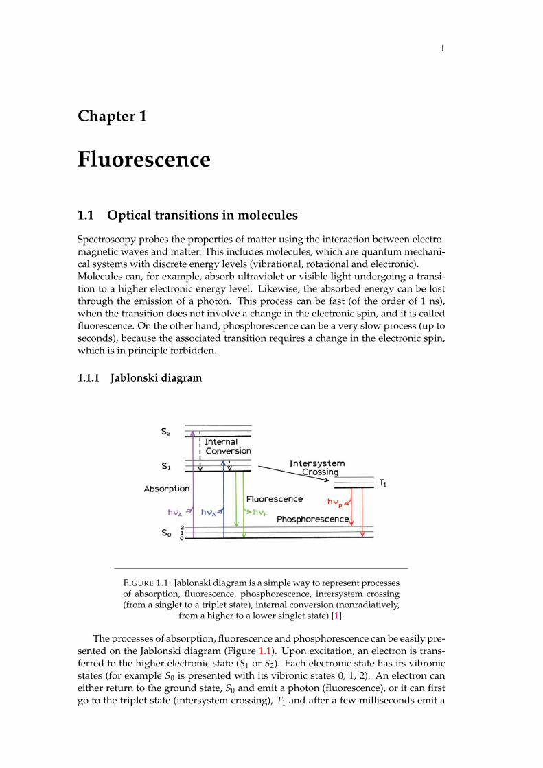
1.1.1 Jablonski diagram

FIGURE 1.1: Jablonski diagram is a simple way to represent processesof absorption, fluorescence, phosphorescence, intersystem crossing(from a singlet to a triplet state), internal conversion (nonradiatively,

from a higher to a lower singlet state) [1].

The processes of absorption, fluorescence and phosphorescence can be easily pre-sented on the Jablonski diagram (Figure 1.1). Upon excitation, an electron is trans-ferred to the higher electronic state (S1 or S2). Each electronic state has its vibronicstates (for example S0 is presented with its vibronic states 0, 1, 2). An electron caneither return to the ground state, S0 and emit a photon (fluorescence), or it can firstgo to the triplet state (intersystem crossing), T1 and after a few milliseconds emit a

2 Chapter 1. Fluorescence

photon (phosphorescence). There is also a possibility that the electron goes back tothe ground state non-radiatively [1].

1.1.2 Fluorescence quantum yield

When a fluorescent molecule absorbs a photon, it can either go back to its groundstate radiatevely or it can loose its energy in the non-radiative process. Fluorescencequantum yield of a molecule represents the ratio of number of emitted and absorbedphotons. This value, depending on the type of molecule can be lower than 1 % orcan be close to 100 %.Another way to define quantum yield is by using the radiative and non-radiativedecay rates, γr and γnr, respectively [2]:

Q =γr

γr + γnr(1.1)

Working with molecules with a high quantum yield has a lot of advantages,mostly due to the fact that the larger number of emitted photons enables easier de-tection.

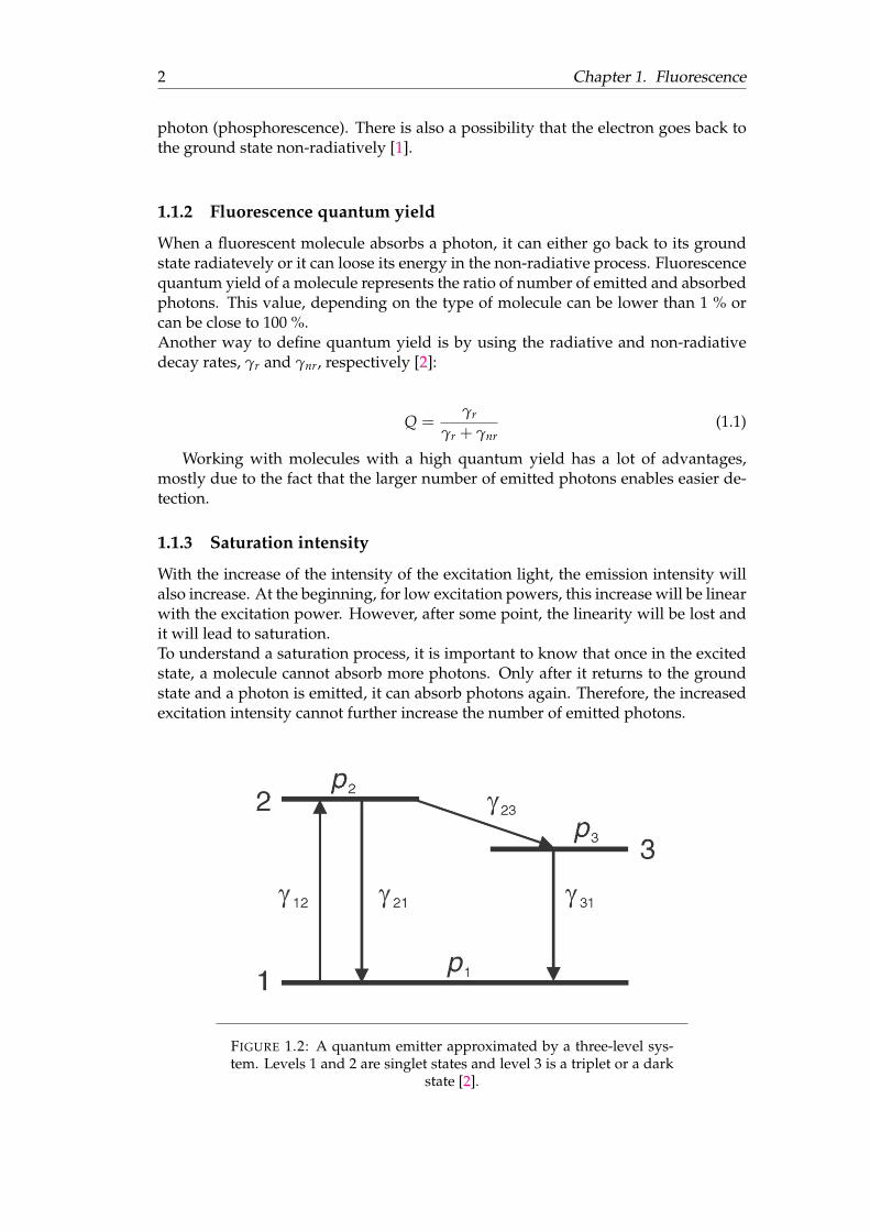
1.1.3 Saturation intensity

With the increase of the intensity of the excitation light, the emission intensity willalso increase. At the beginning, for low excitation powers, this increase will be linearwith the excitation power. However, after some point, the linearity will be lost andit will lead to saturation.To understand a saturation process, it is important to know that once in the excitedstate, a molecule cannot absorb more photons. Only after it returns to the groundstate and a photon is emitted, it can absorb photons again. Therefore, the increasedexcitation intensity cannot further increase the number of emitted photons.

FIGURE 1.2: A quantum emitter approximated by a three-level sys-tem. Levels 1 and 2 are singlet states and level 3 is a triplet or a dark

state [2].

1.1. Optical transitions in molecules 3

A simplified version of the Jablonski diagram is presented in Figure 1.2. Thesinglet ground and the singlet excited states are denoted by numbers 1 and 2, re-spectively. The triplet state is indicated by number 3. These levels are connected bythe excitation and decay rates and one can formulate a system of differential equa-tions (1.2, 1.3, 1.4, 1.5) for the change of the populations p1, p2 and p3. The Equation1.5 states that the emitter has to be in one of the three states at any moment.The absorption process is described by the rate γ12 and the decay from the state 2to the state 1 is described by γ21 = γr + γnr. Likewise, the rates γ23 and γ31 de-scribe transitions from the level 2 to the level 3 and from the level 3 to the level 1,respectively [2].

p1 = −γ12 p1 + (γr + γnr)p2 + γ31 p3 (1.2)

p2 = γ12 p1 − (γr + γnr + γ23)p2 (1.3)

p3 = γ23 p2 − γ31 p3 (1.4)

1 = p1 + p2 + p3 (1.5)

For the steady state, the populations are constant in time and thus their timederivatives are equal to zero (p1, p2, p3 = 0).

The rate at which the system emits photons is given by:

R = p2γr (1.6)

Further calculations brings us to the following relation [2]:

R = R∞

IIs

1 + IIs

(1.7)

The constants R∞ and Is are defined as:

R∞ = γr(1 +γ23

γ31)−1 (1.8)

IS =γr + γnr + γ23

σ(1 + γ23γ31

)hω (1.9)

In Equation 1.9, σ represents the absorption cross-section of a molecule, h is thereduced Planck’s constant (h = 1.05457× 10−34 Js) and ω is the angular frequency ofthe excitation light.

A simple interpretation would be that R∞ represents an emission intensity forthe case in which the excitation intensity is infinite. The excitation intensity at whichthe emission intensity is 50 % of R∞ is the saturation intensity, Is. Measurementsshould be performed under the Is value [2].

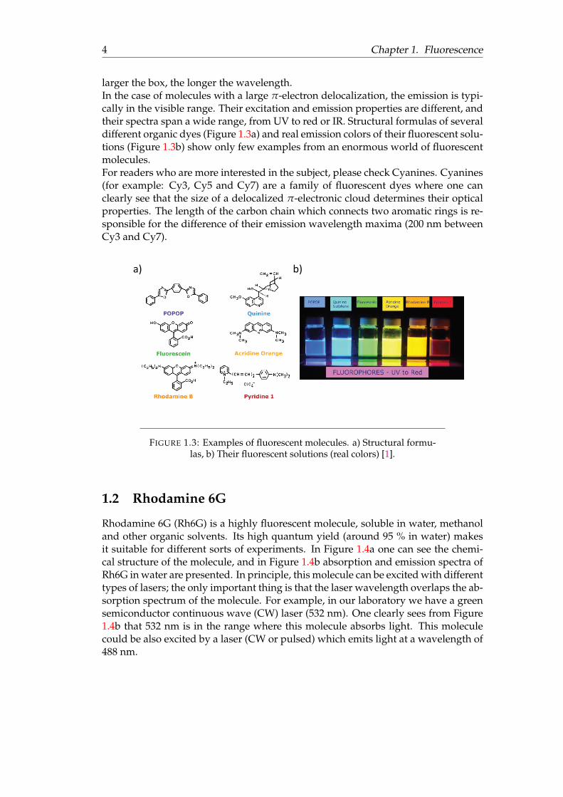
1.1.4 Examples of fluorescent molecules

Fluorescent molecules typically contain aromatic rings with delocalized π-electronsand some examples are shown in the Figure 1.3a. From a quantum mechanical pointof view, a fluorescent molecule can be described as a particle-in-the-box system: the

4 Chapter 1. Fluorescence

larger the box, the longer the wavelength.In the case of molecules with a large π-electron delocalization, the emission is typi-cally in the visible range. Their excitation and emission properties are different, andtheir spectra span a wide range, from UV to red or IR. Structural formulas of severaldifferent organic dyes (Figure 1.3a) and real emission colors of their fluorescent solu-tions (Figure 1.3b) show only few examples from an enormous world of fluorescentmolecules.For readers who are more interested in the subject, please check Cyanines. Cyanines(for example: Cy3, Cy5 and Cy7) are a family of fluorescent dyes where one canclearly see that the size of a delocalized π-electronic cloud determines their opticalproperties. The length of the carbon chain which connects two aromatic rings is re-sponsible for the difference of their emission wavelength maxima (200 nm betweenCy3 and Cy7).

a) b)

FIGURE 1.3: Examples of fluorescent molecules. a) Structural formu-las, b) Their fluorescent solutions (real colors) [1].

1.2 Rhodamine 6G

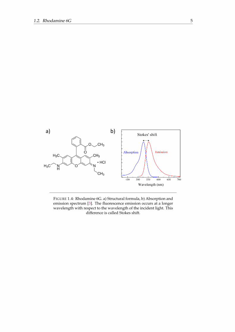
Rhodamine 6G (Rh6G) is a highly fluorescent molecule, soluble in water, methanoland other organic solvents. Its high quantum yield (around 95 % in water) makesit suitable for different sorts of experiments. In Figure 1.4a one can see the chemi-cal structure of the molecule, and in Figure 1.4b absorption and emission spectra ofRh6G in water are presented. In principle, this molecule can be excited with differenttypes of lasers; the only important thing is that the laser wavelength overlaps the ab-sorption spectrum of the molecule. For example, in our laboratory we have a greensemiconductor continuous wave (CW) laser (532 nm). One clearly sees from Figure1.4b that 532 nm is in the range where this molecule absorbs light. This moleculecould be also excited by a laser (CW or pulsed) which emits light at a wavelength of488 nm.

1.2. Rhodamine 6G 5

a) b)

FIGURE 1.4: Rhodamine 6G. a) Structural formula, b) Absorption andemission spectrum [3]. The fluorescence emission occurs at a longerwavelength with respect to the wavelength of the incident light. This

difference is called Stokes shift.

7

Chapter 2

Introduction to FluorescenceCorrelation Spectroscopy

2.1 Auto-correlation and Cross-correlation

Before we explain the principles of FCS, it is important to discuss briefly the mathe-matical apparatus necessary for the interpretation of the data. The auto-correlationof the funcion F is defined as the averaged product of the function value at time t,F(t), with its value after a delay time τ, F(t + τ) [1]:

R(τ) = 〈F(t)F(t + τ)〉 = 1T

∫ T

0F(t)F(t + τ)dt (2.1)

One of the interpretations can be that the auto-correlation function discovers therepetitive pattern in the signal. For example, if we look at a sine or a cosine functions,we can immediately notice some regularities (such as periodicity of the functions).For more complex patterns one must use mathematical tools as mentioned above.

Similarly, a cross-correlation of two different functions, F and P, is defined as :

S(τ) = 〈F(t)P(t + τ)〉 = 1T

∫ T

0F(t)P(t + τ)dt (2.2)

2.1.1 Auto- and Cross-correlation in Fluorescence (Cross-) correlation spec-troscopy

Fluorescence Correlation Spectroscopy (FCS) or Fluorescence Cross-Correlation Spec-troscopy (FCCS) is a technique that is widely used in different fields in order tomonitor processes ranging from simple diffusion in solution to the chemical reac-tions, diffusion of molecules on the membranes and others [1].If you understood the concept of auto- and cross-correlation, it will not be a problemto understand the basics of FC(C)S. More details about the experimental setup willfollow in Chapter 3. For now, it is important to know that the fluorescence is de-tected by photon counters. The number of photons received per second is defined asintensity (F). For convenience, the fluorescence signal can also be split with a 50/50beam splitter and detected by two equal detectors. This is a way to avoid some arti-facts, and will also be discussed later (see afterpulsing in Chapter 3).

The intensity fluctuation, δF around its mean value, 〈F〉, is defined as:

δF = 〈F〉 − F(t) (2.3)

8 Chapter 2. Introduction to Fluorescence Correlation Spectroscopy

The important part is that the intensities detected by the two detectors are recordedon the computer. The auto-correlation of the fluorescence intensity, normalized bythe average intensity squared, is given by [1]:

G′(τ) =〈F(t)F(t + τ)〉〈F〉〈F〉 = 1 +

〈δF(0)δF(τ)〉〈F〉2 (2.4)

In this expression, t is replaced with 0. Some authors consider that working withthe auto-correlation of fluorescence fluctuations is more convenient [1]:

G(τ) =〈δF(0)δF(τ)〉〈F〉2 (2.5)

Similarly a cross-correlation of the intensities and fluorescence fluctuations canbe defined.

9

Chapter 3

Experimental approach to FCS

3.1 Optical setup

In order to examine the fluorescent properties of molecules, there are several maincomponents that are needed. A light source excites emitters and detectors detectfluorescence. There are many types of light sources, such as different lamps, diodesand lasers. In our experiments we will use a semiconductor CW laser and the wave-length of its laser light is 532 nm.The set of mirrors to guide the laser light towards the sample or fluorescent lighttowards detectors, interference filters to reject unwanted scattered or reflected light,objectives to focus light tightly on the sample are only a few among many other op-tical elements present in the optical setup.

3.1.1 Detectors

a) b)

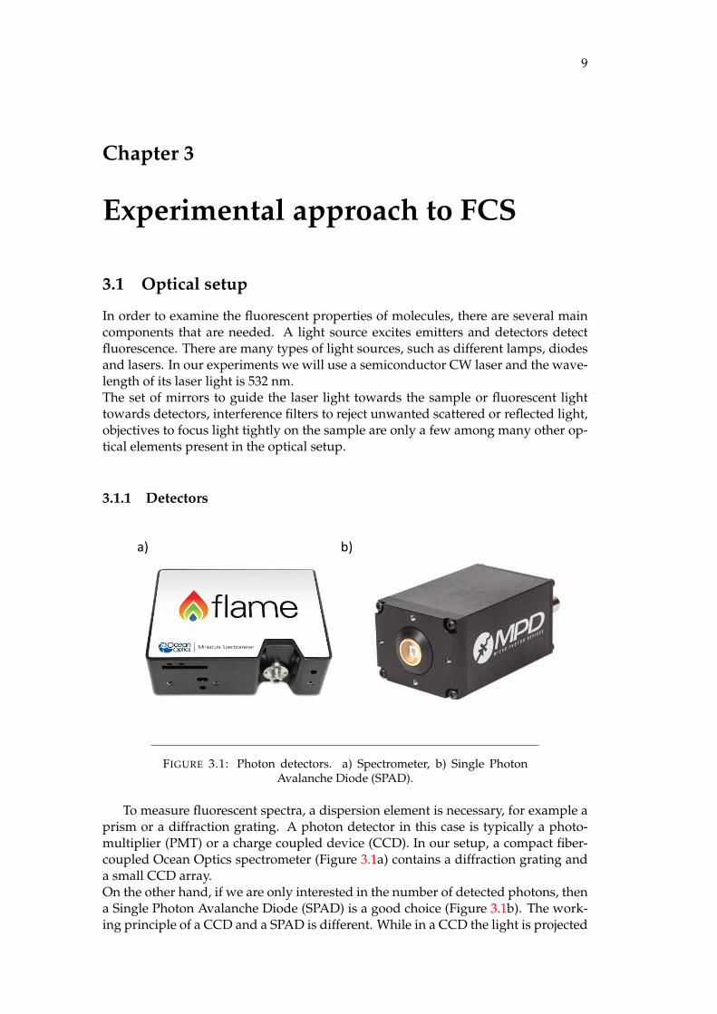
FIGURE 3.1: Photon detectors. a) Spectrometer, b) Single PhotonAvalanche Diode (SPAD).

To measure fluorescent spectra, a dispersion element is necessary, for example aprism or a diffraction grating. A photon detector in this case is typically a photo-multiplier (PMT) or a charge coupled device (CCD). In our setup, a compact fiber-coupled Ocean Optics spectrometer (Figure 3.1a) contains a diffraction grating anda small CCD array.On the other hand, if we are only interested in the number of detected photons, thena Single Photon Avalanche Diode (SPAD) is a good choice (Figure 3.1b). The work-ing principle of a CCD and a SPAD is different. While in a CCD the light is projected

10 Chapter 3. Experimental approach to FCS

on a capacitor array, causing each capacitor to accumulate an electric charge propor-tional to the light intensity at that location, in the SPADs the absorption of a singlephoton is sufficient to generate one electron-hole pair and trigger an avalanche mul-tiplication process [4].

3.1.2 Dark counts and afterpulsing

All detectors have their own internal noise, dark counts, mostly caused by thermaleffects, which produce pulses even in the absence of illumination. The other bigproblem is afterpulsing.It is important to know that these are artifacts and their appearance has nothing todo with the optical properties of the examined emitters.During the avalanche formation, some trapped carriers can get accelerated by theintense electric field across the p-n junction. They further start another avalancheand these new afterpulses are correlated with a previous avalanche pulse [4]. Thisis indeed a huge problem in FCS, since only one detector is used. On the otherhand, this is exactly why it is more convenient to split the fluorescent signal ontwo detectors and perform FCCS. In the cross-correlation, these artifacts will notbe present, since there is no correlation between afterpulsing of the two differentdetectors.

3.1.3 Time Tagged Time-Resolved (TTTR) data collection

The principles of TTTR data collection are explained in detail elsewhere [5]. In orderto examine fluorescence dynamics, it is important to record the arrival times of allphotons with respect to the beginning of the experiment (time tag), and additionallyto record their arrival with respect to the excitation pulse (this holds for a pulsedexcitation).

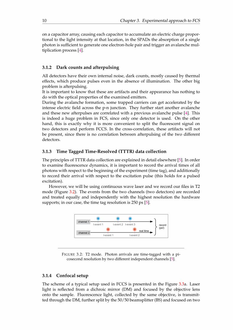
However, we will be using continuous wave laser and we record our files in T2mode (Figure 3.2). The events from the two channels (two detectors) are recordedand treated equally and independently with the highest resolution the hardwaresupports; in our case, the time tag resolution is 250 ps [5].

FIGURE 3.2: T2 mode. Photon arrivals are time-tagged with a pi-cosecond resolution by two different independent channels [5].

3.1.4 Confocal setup

The scheme of a typical setup used in FCCS is presented in the Figure 3.3a. Laserlight is reflected from a dichroic mirror (DM) and focused by the objective lensonto the sample. Fluorescence light, collected by the same objective, is transmit-ted through the DM, further split by the 50/50 beamsplitter (BS) and focused on two

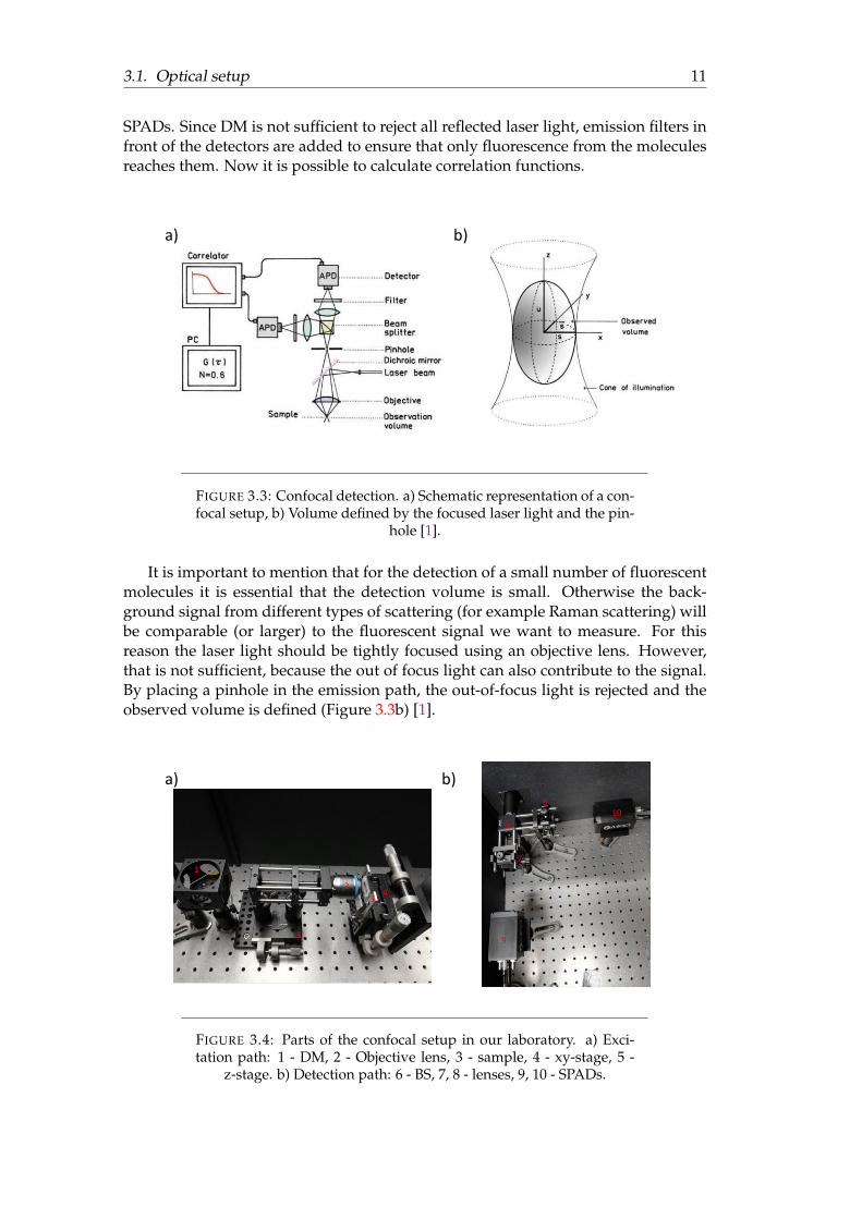
3.1. Optical setup 11

SPADs. Since DM is not sufficient to reject all reflected laser light, emission filters infront of the detectors are added to ensure that only fluorescence from the moleculesreaches them. Now it is possible to calculate correlation functions.

a) b)

FIGURE 3.3: Confocal detection. a) Schematic representation of a con-focal setup, b) Volume defined by the focused laser light and the pin-

hole [1].

It is important to mention that for the detection of a small number of fluorescentmolecules it is essential that the detection volume is small. Otherwise the back-ground signal from different types of scattering (for example Raman scattering) willbe comparable (or larger) to the fluorescent signal we want to measure. For thisreason the laser light should be tightly focused using an objective lens. However,that is not sufficient, because the out of focus light can also contribute to the signal.By placing a pinhole in the emission path, the out-of-focus light is rejected and theobserved volume is defined (Figure 3.3b) [1].

a) b)

1

2

34

5

6

7

8

9

10

FIGURE 3.4: Parts of the confocal setup in our laboratory. a) Exci-tation path: 1 - DM, 2 - Objective lens, 3 - sample, 4 - xy-stage, 5 -

z-stage. b) Detection path: 6 - BS, 7, 8 - lenses, 9, 10 - SPADs.

12 Chapter 3. Experimental approach to FCS

The parts of the experimental setup from our lab are presented in Figure 3.4.One part of the excitation path is presented in Figure 3.4a: light reflected by theDM is directed through the objective lens onto the sample. The sample stage can becontrolled in the x and y directions. The z-stage is used to focus light transmittedthrough the objective lens.

A photo of the detection path with SPADs is shown in Figure 3.4b. Light reflectedfrom the BS is further focused by the lenses on two SPADs.

3.1.5 Confocal volume - geometrical interpretation

Confocal volume is defined by the properties of the setup, mainly by the wavelengthof the laser and the properties of the objective lens. There is a limit up to which onecan focus a Gaussian beam. According to scalar diffraction theory, the resolution inthe xy-plane is:

rxy =0.61λ

NA(3.1)

The resolution in the z-direction is given by:

rz =2nλ

NA2 (3.2)

In these equations, λ represents the laser wavelength, NA is a numerical aper-ture of the objective lens, and n is the index of refraction of the medium in which theemitters are dissolved. The numerical aperture is one of the most important char-acteristics of a microscope objective and it is given by a dimensionless number thatcharacterizes the range of angles over which the objective lens can accept or emitlight.

The pinhole is small enough to reject out-of-focus light, but large enough to passthe light from the illumination spot. A three-dimensional Gaussian can approximatethe profile associated with the confocal volume presented in Figure 3.3b [1]:

p(r) = I0e−2 x2+y2

s2 e−2 z2

u2 (3.3)

In this case, the radius s and half-length u define distances at which the intensitydecreases to e−2 of its maximal value.In practice, there are several ways to determine the size and the shape of the confocalvolume. One of the best known and widely used is to perform a 3D scan of a singlefluorescent bead whose size is much smaller than the diffraction limit [6].

13

Chapter 4

FCCS and Diffusion

4.1 Diffusion

Molecules and other particles move randomly in solutions. This kind of process iswell known as Brownian motion. The diffusion of molecules represents their ther-mal motion and depends on the molecule size and its interaction with the environ-ment.To calculate an auto-correlation function for isotropic, three dimensional diffusion,we should start from the basic laws of diffusion. First, we should define the con-centration as the number of molecules divided by the product of the observationvolume and the Avogrado’s number, NA (NA = 6.022 141 29× 1023 mol−1).The local concentration, C(~r, t) can be expressed as a sum of the average concentra-tion, 〈C〉 and the diffusion-driven stochastic fluctuation of the concentration, δC(~r, t):

C(~r, t) = 〈C〉+ δC(~r, t) (4.1)

Further, the fluctuations change according to Fick’s law [7]:

∂δC(~r, t)∂t

= D∇2δC(~r, t) (4.2)

The detailed solving of all differential equations is beyond our scope. At thispoint we will focus on their solutions. For further reading, please refer to Refer-ence [8].

The correlation function for the diffusion in three dimensions has this form [1]:

G(τ) = G(0)(1 +τ

τD)−1(1 + (

su)2 τ

τD)−

12 (4.3)

The diffusion time, τD is dependent on the size of the detection volume and thediffusion coefficient D [1]:

τD =s2

4D(4.4)

The diffusion coefficient, on the other hand, depends on the temperature T, theviscosity of the medium in which molecules move η, and their hydrodynamic ra-dius, r:

D =kT

6πηr(4.5)

where k represents the Boltzmann’s constant (k = 1.381× 10−23 J K−1).

14 Chapter 4. FCCS and Diffusion

If we fit the correlation function given by Equation 4.3, one parameter that weobtain is the diffusion time, τD. The other parameter is G(0), and it is inversely-proportional to the average number of molecules in the detection volume [1]:

G(0) =1N

(4.6)

For known sample concentration, one can easily determine the effective volume,Ve f f :

Ve f f =N

NA〈C〉(4.7)

Here NA represents the Avogadro’s number.

4.1.1 Interpretation of the equations

It is not easy to understand immediately how to interpret the quantities obtainedfrom the correlation curve. Given the fact that the theory of FCS is based on the Pois-son statistics, the number of fluorescent molecules in the volume can be describedby the Poisson distribution [1]:

P(n, N) =Nn

n!e−N (4.8)

P(n, N) represents the probability that n molecules are present in the volume,when the average number in the volume is N. For example, if N = 0.6, that meansthat the probability that there are no molecules in the volume is 55%. To have onlyone molecule present, the probability is 33%. And for two molecules present at thesame time in the volume, the probability drops to only 10% [1].

The diffusion time is a quantity that depends on the geometry of the volume, asgiven in Equation 4.4; the larger the radius, the larger the diffusion time. That simplymeans that τD is not a good quantity to be taken as a reference, since every setupwill have a slightly different shape of the detection volume. However, the diffusioncoefficient should be constant if the samples are kept under the same experimentalconditions (temperature, viscosity).

15

Chapter 5

Instructions for measurements

5.1 Measurements

In this Chapter we will present many technical details. Namely, the main ideas havealready been presented. However, every optical setup is slightly different and alsothe Software used for the data collection and processing can vary significantly. ThisChapter is more like a cookbook; it is here to guide you through the experiments. Byfollowing the instructions you can perform measurements, save and process data.

5.1.1 Samples

We will examine Rhodamine 6G molecules in water and water/glycerol mixtures.The movement of molecules depends strongly on the viscosity of the medium. Thehigher the percentage of glycerol, the more viscous the environment would be andthus the slower the movement. These solutions will be sealed in the home madeflow chambers to prevent an evaporation and leakage of the sample. Teaching assis-tants will take care of the sample preparation before the experiment takes place.For all measurements, the first step would be clamping the sample to the samplestage. The sample stage can be moved in the x-y plane using micrometer screws.However, in order to focus light, one should move the objective which is on a sepa-rate micrometer stage and can translate along the z-axis (Figure 3.4).

5.1.2 Measurements of fluorescence spectra

In the optical setup the fiber-coupled spectrometer is not in the main optical path.There is a flip-mirror which will steer the emitted light in the direction of the opticalfiber. Maybe small adjustments of the mirror are needed to improve the couplingwith the optical fiber.

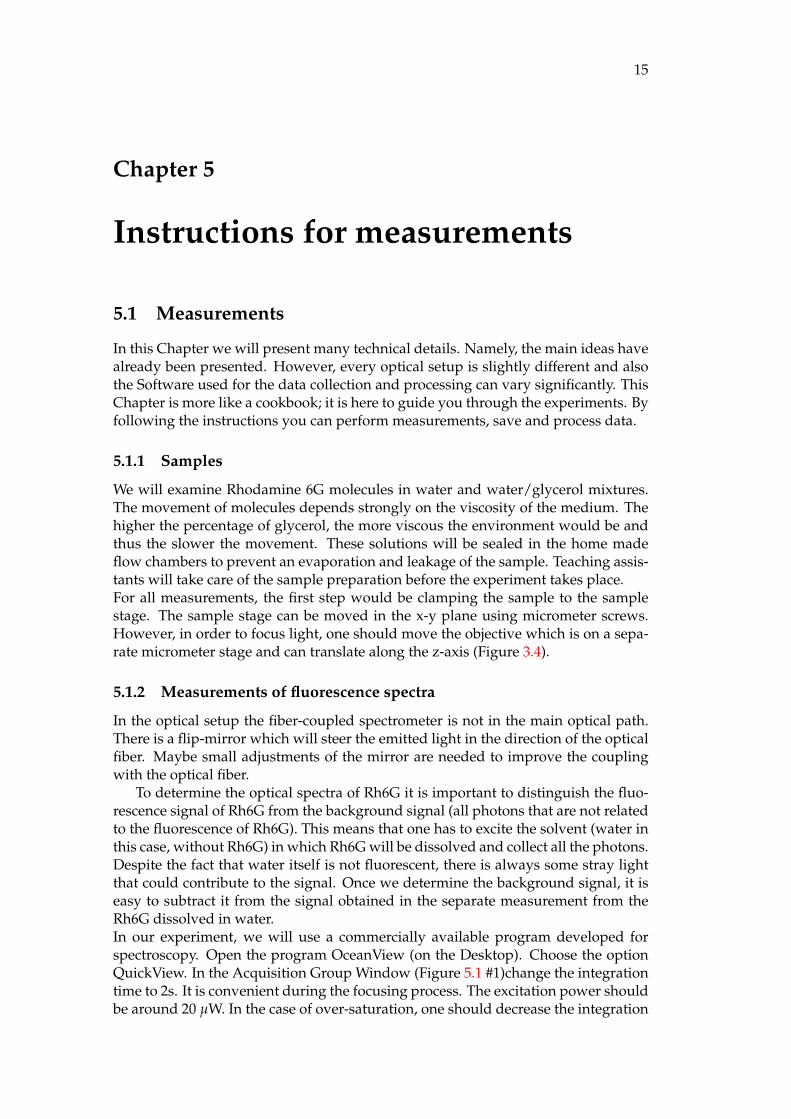
To determine the optical spectra of Rh6G it is important to distinguish the fluo-rescence signal of Rh6G from the background signal (all photons that are not relatedto the fluorescence of Rh6G). This means that one has to excite the solvent (water inthis case, without Rh6G) in which Rh6G will be dissolved and collect all the photons.Despite the fact that water itself is not fluorescent, there is always some stray lightthat could contribute to the signal. Once we determine the background signal, it iseasy to subtract it from the signal obtained in the separate measurement from theRh6G dissolved in water.In our experiment, we will use a commercially available program developed forspectroscopy. Open the program OceanView (on the Desktop). Choose the optionQuickView. In the Acquisition Group Window (Figure 5.1 #1)change the integrationtime to 2s. It is convenient during the focusing process. The excitation power shouldbe around 20 µW. In the case of over-saturation, one should decrease the integration

16 Chapter 5. Instructions for measurements

1 23

FIGURE 5.1: OceanView software. By clicking on the AcquisitionGroup Window #1, one can choose the desired integration time. Graybulb #2, is for a background subtraction. To copy the data on the clip-

board, one should click on the icon designated by #3.

time to 0.5 s. In order to perform a measurement, once everything is aligned, thelaser should be blocked and the gray light bulb should be pressed (Figure 5.1 #2).After the laser light is unblocked and the sample is illuminated, one obtains a flu-orescent signal. Choose the icon to copy the data on the clipboard (Figure 5.1 #3).Open the Notepad and paste the data (CTRL+V). It is important to remove the firstline of letters not to cause some issues while loading the file in Python for example.Save the data!

5.1.3 Correlation curves

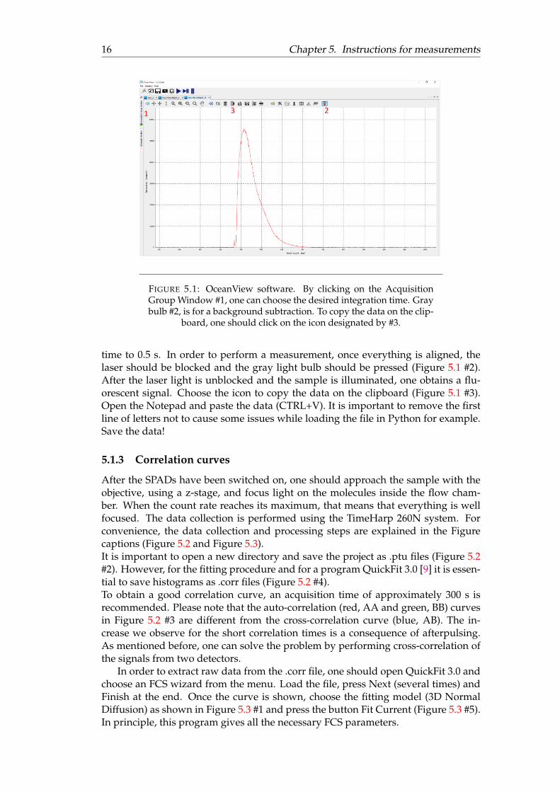
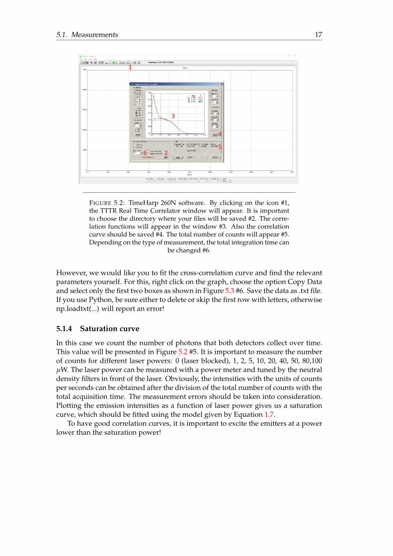
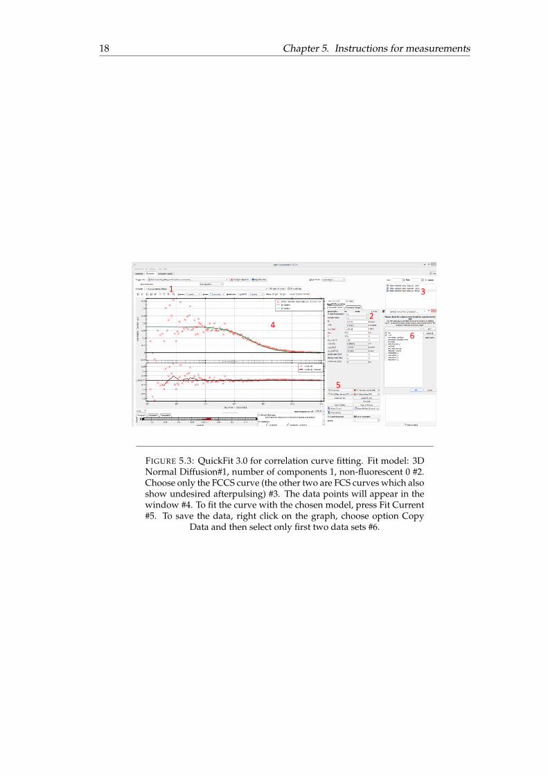
After the SPADs have been switched on, one should approach the sample with theobjective, using a z-stage, and focus light on the molecules inside the flow cham-ber. When the count rate reaches its maximum, that means that everything is wellfocused. The data collection is performed using the TimeHarp 260N system. Forconvenience, the data collection and processing steps are explained in the Figurecaptions (Figure 5.2 and Figure 5.3).It is important to open a new directory and save the project as .ptu files (Figure 5.2#2). However, for the fitting procedure and for a program QuickFit 3.0 [9] it is essen-tial to save histograms as .corr files (Figure 5.2 #4).To obtain a good correlation curve, an acquisition time of approximately 300 s isrecommended. Please note that the auto-correlation (red, AA and green, BB) curvesin Figure 5.2 #3 are different from the cross-correlation curve (blue, AB). The in-crease we observe for the short correlation times is a consequence of afterpulsing.As mentioned before, one can solve the problem by performing cross-correlation ofthe signals from two detectors.

In order to extract raw data from the .corr file, one should open QuickFit 3.0 andchoose an FCS wizard from the menu. Load the file, press Next (several times) andFinish at the end. Once the curve is shown, choose the fitting model (3D NormalDiffusion) as shown in Figure 5.3 #1 and press the button Fit Current (Figure 5.3 #5).In principle, this program gives all the necessary FCS parameters.

5.1. Measurements 17

1

2

3

4

56

FIGURE 5.2: TimeHarp 260N software. By clicking on the icon #1,the TTTR Real Time Correlator window will appear. It is importantto choose the directory where your files will be saved #2. The corre-lation functions will appear in the window #3. Also the correlationcurve should be saved #4. The total number of counts will appear #5.Depending on the type of measurement, the total integration time can

be changed #6.

However, we would like you to fit the cross-correlation curve and find the relevantparameters yourself. For this, right click on the graph, choose the option Copy Dataand select only the first two boxes as shown in Figure 5.3 #6. Save the data as .txt file.If you use Python, be sure either to delete or skip the first row with letters, otherwisenp.loadtxt(...) will report an error!

5.1.4 Saturation curve

In this case we count the number of photons that both detectors collect over time.This value will be presented in Figure 5.2 #5. It is important to measure the numberof counts for different laser powers: 0 (laser blocked), 1, 2, 5, 10, 20, 40, 50, 80,100µW. The laser power can be measured with a power meter and tuned by the neutraldensity filters in front of the laser. Obviously, the intensities with the units of countsper seconds can be obtained after the division of the total number of counts with thetotal acquisition time. The measurement errors should be taken into consideration.Plotting the emission intensities as a function of laser power gives us a saturationcurve, which should be fitted using the model given by Equation 1.7.

To have good correlation curves, it is important to excite the emitters at a powerlower than the saturation power!

18 Chapter 5. Instructions for measurements

1

2

3

4

5

6

FIGURE 5.3: QuickFit 3.0 for correlation curve fitting. Fit model: 3DNormal Diffusion#1, number of components 1, non-fluorescent 0 #2.Choose only the FCCS curve (the other two are FCS curves which alsoshow undesired afterpulsing) #3. The data points will appear in thewindow #4. To fit the curve with the chosen model, press Fit Current#5. To save the data, right click on the graph, choose option Copy

Data and then select only first two data sets #6.

19

Chapter 6

Students’ tasks

6.1 Tasks

1. Calculation of the confocal volume based on Equations 3.1 and 3.2 for the op-tical system in the laboratory (the numerical aperture of the objective lens isNA = 0.6 and λ = 532nm).

2. Measurements of the emission spectrum for a high concentration of Rh6Gmolecules. Plot the emission spectra and make a comment on the curve shape.How is it related to the shape presented in Figure 1.4?

3. Measurement of the saturation curve for a known concentration of Rh6G inwater, fitting the data using the model given by Equation1.7 and obtainingR∞ and Is from the fit. For the saturation curve fitting, 10 data points wouldbe sufficient, as suggested in Chapter 5. To estimate the average values andmeasurement errors, it is recommended to collect photons for 30 s and to repeatthe same measurement five times. This is a good approach to get an averagevalue with the corresponding error.

4. Estimation of the effective volume based on the results obtained from the FCCScurves for a sample of known concentration. Please compare this value withthe calculated value. To calculate the effective volume, you can use Equation4.7.

5. FCCS measurements of Rh6G dissolved in a mixture of water and glycerol.The goal is to compare the diffusion times and show that they increase withthe increase of a glycerol content in the mixture. Five samples will be pre-pared with different ratios of water and glycerol: 100 % H2O; 75 % H2O, 25 %glycerol; 50 % H2O, 50 % glycerol; 25 % H2O, 75 % glycerol; 10 % H2O, 90 %glycerol.

6.2 Output

1. A good report should be clearly structured. Split it into several parts: Ab-stract, Introduction, Theory, Experimental Section, Data analysis, Discussionand Conclusions.

2. Figures should have figure captions with explanations. All graphs should havelabeled axes and visible data points and curves. Curve fits and fitted parame-ters should be included.

3. All quantities should be followed by the calculated error.

20 Chapter 6. Students’ tasks

4. It is important to use your own words to explain what you observe in theexperiment and to interpret the data. Graphs and numbers without interpre-tation are not sufficient.

If at any point during your data processing or report writing you have anydoubts, you are encouraged to contact your teaching assistants. We are more thanhappy to help you finish your task and learn as much as possible.

We wish you good luck with experiments!

21

Bibliography

[1] J. R. Lakowicz, “Principles of fluorescence spectroscopy, 3rd edition”, Springer-Verlag US 2006, 2006. [Online]. Available: http://link.aip.org/link/?RSI/62/1/1.

[2] L. Novotny and B. Hecht, “Principles of nano-optics”, Cambridge UniversityPress, 2006. [Online]. Available: https://doi.org/10.1017/CBO9780511813535.

[3] M. Duteil, “Collective behaviour - from cells to humans”, PhD thesis, 2019. [On-line]. Available: 10.23889/Suthesis.50750.

[4] “Micro photon devices”, [Online]. Available: http : / / www . micro - photon -devices.com/Products.

[5] M. Wahl and S. Orthaus-Müller, “Time tagged time-resolved fluorescence datacollection in life sciences”, PicoQuant GmbH, 2015. [Online]. Available: https://www.picoquant.com/images/uploads/page/files/14528/technote_tttr.

pdf.

[6] V. B. et al., “Quantitative fcs: Determination of the confocal volume by fcs andbead scanning with the microtime200”, PicoQuant GmbH, 2009. [Online]. Avail-able: https://www.picoquant.com/images/uploads/page/files/7351/appnote_quantfcs.pdf.

[7] “Fcs classroom”, [Online]. Available: http://www.fcsxpert.com/classroom/.

[8] E. L. Elson and D. Magde, “Fluorescence correlation spectroscopy. i. conceptualbasis and theory”, Biopolymers, vol. 13, 1974. [Online]. Available: https://doi.org/10.1002/bip.1974.360130102.

[9] “Quickfit 3.0”, [Online]. Available: https://www.dkfz.de/Macromol/quickfit/.