Fluorescence lifetime imaging for the two-photon ... · Fluorescence lifetime imaging for the two-photon microscope: time-domain and frequency-domain methods ... Journal of Biomedical

Fluorescence lifetime imaging for the two-photonmicroscope: time-domain and frequency-domainmethods

Enrico GrattonSophie BreusegemJason SutinQiaoqiao RuanNicholas BarryUniversity of Illinois at Urbana-ChampaignLaboratory for Fluorescence Dynamics1110 West Green StreetUrbana, Illinois 61801E-mail: [email protected]

Abstract. Fluorescence lifetime images are obtained with the laserscanning microscope using two methods: the time-correlated single-photon counting method and the frequency-domain method. In thesame microscope system, we implement both methods. We perform acomparison of the performance of the two approaches in terms ofsignal-to-noise ratio (SNR) and the speed of data acquisition. While inour practical implementation the time-correlated single-photon count-ing technique provides a better SNR for low-intensity images, thefrequency-domain method is faster and provides less distortion forbright samples. © 2003 Society of Photo-Optical Instrumentation Engineers.[DOI: 10.1117/1.1586704]

Keywords: fluorescence lifetime imaging; frequency domain; time domain; two-photon microscopy.

Paper MM-15 received Apr. 8, 2003; revised manuscript received Apr. 10, 2003;accepted for publication Apr. 10, 2003.

1 IntroductionIn complement with the emission spectrum, the determinationof the lifetime of the excited state is a commonly used tech-nique to characterize the emitting molecular species. In thecontext of fluorescence microscopy, fluorescence lifetime im-aging �FLI� can provide a new contrast mechanism to helpidentify the local environment of the fluorophore. In addition,FLI can enable the quantitation of the relative concentrationof a number of species that are colocalized. FLI has beendeveloped in several laboratories.1–24 Among the most com-mon applications is the determination of ion or other smallligand concentration using lifetime-sensitive dyes, the deter-mination of oxygen concentration in cells and the quantitationof Forster resonance energy transfer �FRET� for distance mea-surements in the nanometer range.

Two alternative methods are primarily used for the mea-surement of the fluorescence lifetime. One method is referredto as the time-domain method and it is based on constructingthe histogram of photon delays using the time-correlatedsingle-photon counting �TCSPC� method. The other method isgenerally referred to as the frequency-domain method and itconsists of measuring the harmonic response of a fluorescentsystem using either sinusoidally modulated excitation light ora fast repetition pulse train laser. The TCSPC method is in-trinsically a digital method wherein the detector measures onephoton at the time. However, the time delay is measured usingan analog detection method �time to amplitude converter� fol-lowed by fast conversion to a digital form. The frequency-domain method is intrinsically an analog method �althoughthe waveform is digitally recorded� and the detector delivers acurrent proportional to the light intensity. These two differentmethods have been extensively described in the literature inconnection to measurements of fluorescence lifetime in a cu-vette and we will not review the principles in this paper. Forthe interested reader, we suggest a number of review articlesor books included in the references �see for example the series

of Topics in Fluorescence Spectroscopy25–27�. More recently,both methods have also been used for the determination offluorescence lifetime in the microscope environment.28–32 Inthis paper, we discuss our implementation of lifetime mea-surements in the laser-scanning microscope using bothfrequency- and time-domain methods and the comparison be-tween them. Lifetime measurements in the microscope usingtime-resolved cameras have also been previously discussed�see, for example, Refs. 12 and 14�. Since the camera per secannot provide the time resolution required for fluorescencelifetime measurements, these devices are generally used inconjunction with an image intensifier that acts as a fast shut-ter. This shutter can be thought of as a modulation of the gainof the detection system and in our classification falls under thegeneral category of the analog detection mode. The sameprinciple, namely, the modulation of the gain of the detector,can be used in a single-channel detector. Note here that thekind of gain modulation that is applied to the detector doesnot change the analog nature of the detection system. There-fore, rather arbitrarily, we will also include in the category offrequency-domain detection these methods that employ a nar-row opening of the detector gain to sample the decay curvesome time after the excitation. In practice, this scheme ofmodulation increases the harmonic content of the detectedsignal at the expense of the duty cycle. The advantages of thisapproach were previously described, for both cuvette experi-ments and the microscopy environment.19,33 In this paper, wediscuss only sinusoidal modulation of the detector gain, al-though the use of other functions could offer significant ad-vantages when the sample contains multiple species with dif-ferent lifetimes.

The lifetime approach in imaging is generally differentfrom that in the cuvette. In a cuvette measurement, we areinterested in the accurate measurement of the fluorescence

1083-3668/2003/$15.00 © 2003 SPIE

Journal of Biomedical Optics 8(3), 381–390 (July 2003)

Journal of Biomedical Optics � July 2003 � Vol. 8 No. 3 381

decay with the purpose of determining the number of differentcomponent species contributing to the decay or specificmechanisms involved in the deactivation of the excited state.In imaging, we are interested in resolving one or two compo-nents and in using the lifetime parameters as a means to con-trast the image or to determine the locations in the image inwhich a specific excited state reaction occurs. Therefore, theinstrumentation for lifetime measurements in a cuvette differssomewhat from that used for imaging.

The problem of determining the fluorescence lifetime dur-ing the small time the laser scans a pixel in the image issimilar to the problem of determining the lifetime during astopped-flow measurement or in the flow-cytometerenvironment.24 However, in both the stopped-flow and theflow cytometer, a relatively large fluorescence signal is mea-sured. For example, in the flow cytometer, the fluorescence iscollected from an entire cell, while in FLI the fluorescence iscollected from each pixel of the image. A pixel is generallymuch smaller than a cell and, more importantly, containsfewer fluorophores. Another area of recent development isrelated to the measurement of the fluorescence lifetime ofsingle molecules, either immobilized or freely diffusing insolution. The challenge of the lifetime determination duringvery short acquisition times can be expressed in terms of thetotal intensity collected during a small amount of time. Thepurpose of this study is to determine the various regimes ofoperation and to perform experimental observations to deter-mine how the best SNR can be obtained for the two differentlifetime approaches �digital versus analog�.

For this purpose we assembled a laser-scanning micro-scope system34,35 based on two-photon excitation36–39 inwhich we can make lifetime measurements using both tech-niques with acquisition times as short as 50 �s. We describe anew analysis of the frequency- and time-domain methods inthe same microscope so that a meaningful comparison be-tween the two methods could be achieved. We first presentsimulation experiments to demonstrate the analysis techniqueand to illustrate the effect of photon-counting statistics on theprecision of lifetime measurement. We then compare the twoapproaches, using cuvette-type experiments with a homoge-neous solution sample and stationary excitation beam. Finally,lifetime images are presented.

Although the light source, sample, and microscope are thesame in our system, the detectors used for the time domainand the frequency domain are different. In the frequency do-main, we used the Hamamatsu R928 photomultiplier with rfmodulation at the second dynode, while in the time-domainexperiments we used the Hamamatsu R7400, wired forphoton-counting operation.

To perform a comparison between the two methods for thecuvette experiments, we transformed the time-domain decayto the frequency domain by calculating the fast Fourier trans-form �FFT� of the time decay data so that the measurementscould be directly compared in terms of phase and modulationaccuracy. However, data analysis to recover the decay param-eters for the time-domain data was also performed directly inthe time domain to preserve the proper information about thedata statistics.

For the imaging experiments, again we transformed thetime-domain decay to the frequency domain for each pixel.This operation enables the use of analytical expressions for

the lifetime of a multicomponent system. This is an importantdifference in our implementation, since the literature for thetime-domain approach in FLI describes the use of look-uptables and other semiempirical techniques to recover the life-time of multiple components.8

A conclusion of our study is the rather obvious observationthat the quality of the recovered data depends only on theSNR, which is essentially determined by the number of pho-tons collected in both the time and the frequency domains.When the light intensity is relatively large, over106 photons/s, the digital method of data acquisition intrinsi-cally limits the rate of photon acquisition in the time domain.Since in the frequency domain, the detection system operatesin the analog mode, this limitation does not occur. This is animportant consideration for FLI, as explained later in this pa-per. For very low signal intensity, the discrimination capabil-ity of the single-photon-counting method provides a betterSNR. However, other factors play an important role in im-proving the SNR at low-light-intensity levels in the frequencydomain.

2 Experimental Setup2.1 Cuvette SetupAll experiments were performed using a two-photon excita-tion microscope with a 1.3 numerical aperture �NA� oil objec-tive. For the cuvette experiments, we used an eight-well slideholder with two wells filled with the sample and the referencesolution, respectively. In the sample well, we made a dilutionstudy of fluorescein in PBS buffer at pH 8 over the range from1 nM to 100 �M. A fixed excitation power was used such thata large range of emission intensities were measured. In thereference well, we used solution of dimethyl-POPOP �lifetime1.45 ns�. The excitation source was a Tsunami mode-lockedtitanium:sapphire laser �Spectra Physics, Sunnyvale, Califor-nia� with a repetition frequency of 80 MHz and a pulse widthof about 100 fs. The optical path for the two-photon systemhas a dichroic mirror to separate the excitation light �generallyin the 800-nm region� from the emission �in the interval 450to 700 nm�. In front of the detector, we used a filter �BG39,Schott glass� to block the scattered light �and/or second-harmonic generation �SHG�� at the near-IR excitation wave-length. For the cuvette experiments, the beam was held sta-tionary at the center of the cuvette.

2.2 Microscope SetupThe experimental setup is essentially the same used for thecuvette experiment, but the sample consists of a cell that ex-presses the enhanced green fluorescent protein �EGFP�. In thiscase, the laser beam was raster-scanned across the sample toobtain an image 256�256-pixels wide with a residence timeof about 200 �s/pixel. In some cases, several images wereaveraged to obtain an effective larger count per pixel.

3 Simulation ExperimentsThe purpose of this section is to determine how the total num-ber of counts affects the recovered lifetime in the regime ofrelatively few counts in the decay curve and to test the meth-ods of recovering the lifetime value under this condition usingthe FFT of the time-domain data. All simulations were per-

Gratton et al.

382 Journal of Biomedical Optics � July 2003 � Vol. 8 No. 3

formed in the time domain, but the data were processed andbinned as if they were acquired in a frequency-domain instru-ment. The FFT method has been extensively used in the de-convolution of the lamp response for time-domain analysis.40

It is no longer used due to the speed of computation of mod-ern computers and because, for the FFT operation, it is diffi-cult to correctly propagate the statistics. In the FLI context,we propose this approach because it is fast and provides arelatively simple way to recover pixel lifetime values up totwo to three components.41,42

Simulations were performed to mimic the emission of asolution 10 nM of fluorescein, which under normal circum-stances in our instrument, shows a single exponential decay ofabout 4 ns. The count rate for this sample �which ultimatelywill depend on the laser power and the collection optics� wassimulated to be about 4 kHz, which is adequate for obtaininggood statistics in both frequency- and time-domain techniquesin cuvette-type experiments.

First, we show the principle of the method in a single-channel simulated experiment. A typical simulated decay offluorescein �4 ns, blue dots� and for the decay of a theoreticalstandard compound �1.0 ns, green dot� is shown in Fig. 1. A fitobtained using standard time-domain analysis8 is shown inFig. 1 �solid lines�. For this simulation, the sample curve con-tains about 4000 counts and the reference curve has about2000 counts.

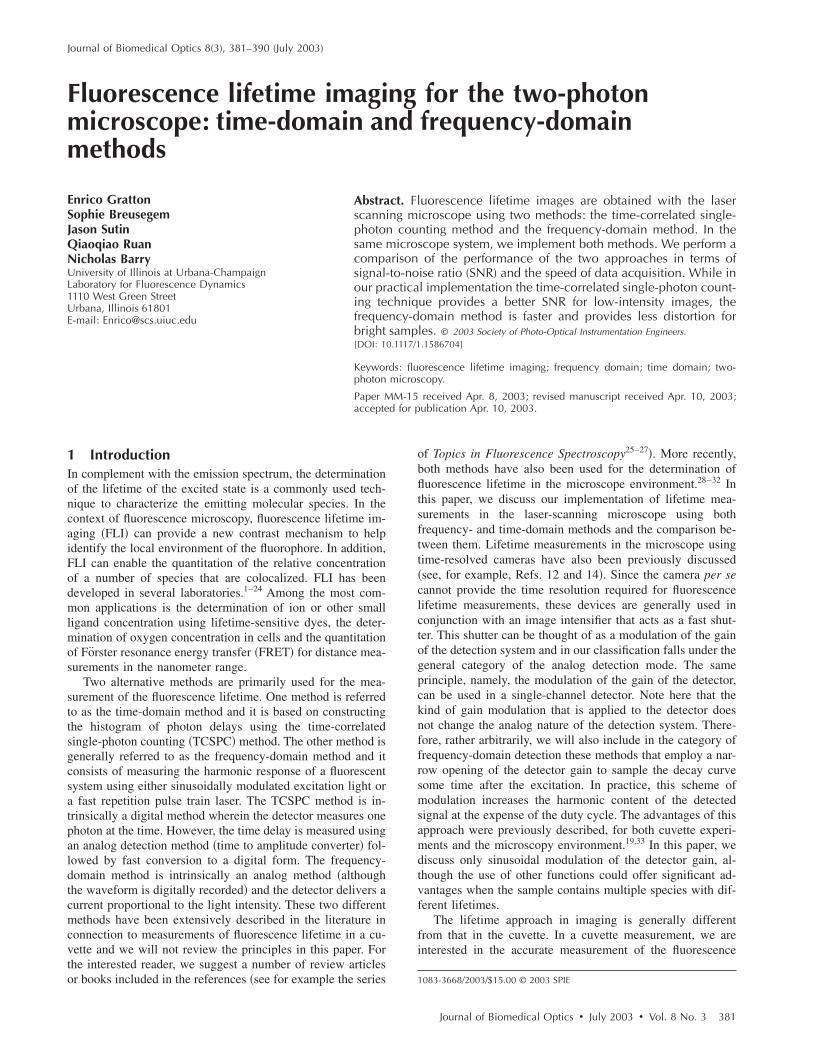
The recovered result is 4.2�0.1 and 0.94�0.05 ns for asingle exponential component resolution of the decay. Thesimulated raw data set was fast Fourier transformed and it ispresented in a typical frequency-domain format in Fig. 2. TheFT �real and imaginary parts converted to phase and modula-tion values� of the sample and reference decays are shown inFig. 2 in a log frequency axis for the 4-ns �red symbols� andthe 1-ns �blue symbols� decays, respectively.

The modulation curve for both decays is relatively smoothand close to the expected value �solid lines� up to about 1000MHz. Instead, the phase curve shows large deviations fromthe expected monotonically increasing curve starting at about80 MHZ. However, if we calculate the relative phase betweenthe two signals corrected for the finite lifetime of the refer-

ence and the modulation ratio �corrected also for the lifetimeof the reference� we obtain the points �green points� of Fig. 2.The relative phase and the modulation ratio follow the ex-pected trend up to about 1000 MHz. This simulation showsthat the deconvolution of the lamp response �approximately300 ps for the Hamamatsu R7400 detector used in this study�is necessary to correctly recover the decay even for the rela-tively narrow lamp pulse used for this simulation.

Using the Globals WE software program �Laboratory forFluorescence Dynamics, University of Illinois�, we analyzedthe phase and modulation curves obtained from the time-domain data after referencing and we obtained the fit shownin Fig. 2.

The recovered lifetime is 4.3�0.1 ns, in good agreementwith the time-domain analysis of the same original data set.However, the residues are larger than 2 to 3 deg on the low-frequency part of the curve and they increase in the high-frequency part. It is clear that the residues are quite large forstandard frequency-domain data and that the overall fit isgood only up about 100 MHz. This simulation shows thateven for a decay curve containing on the order of 4000counts, the frequency range available is limited to about 100MHz. In summary, this analysis method shows the usefulbandwidth of a time-domain measurement given a particularnumber of photons collected.

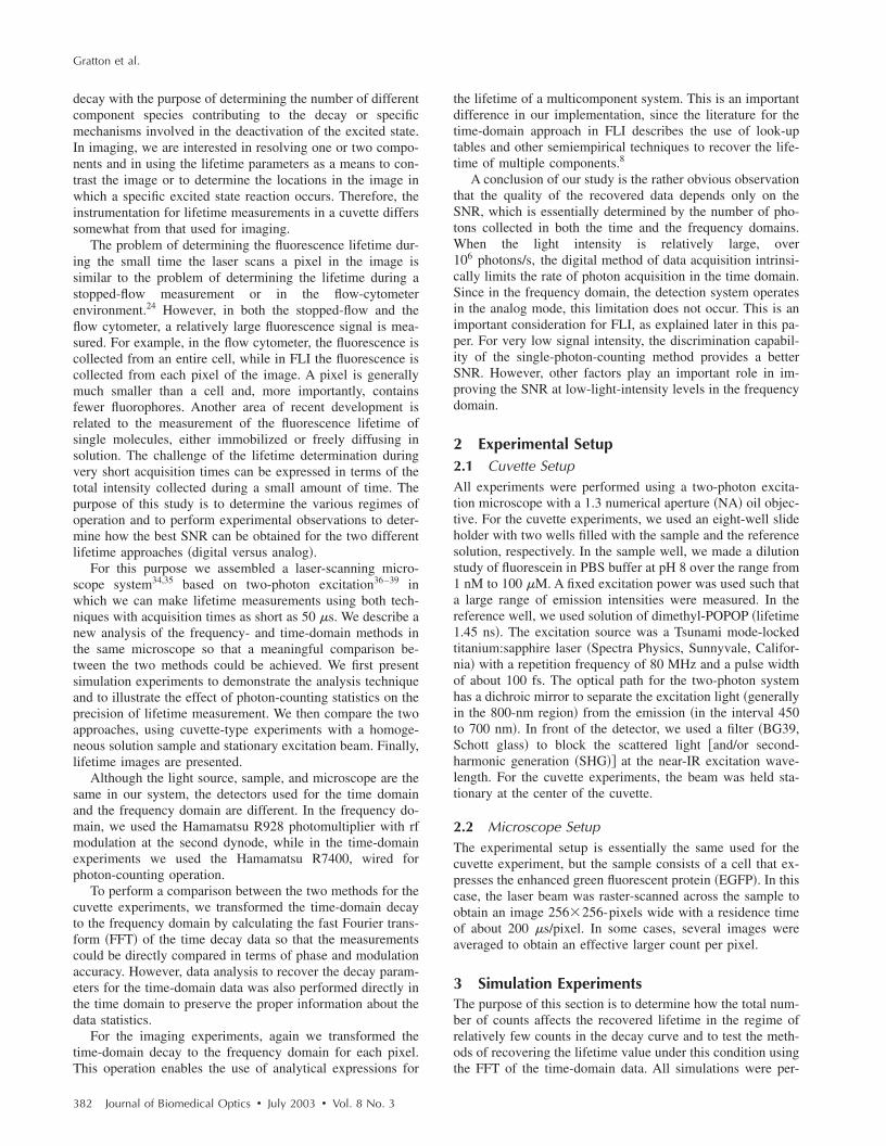
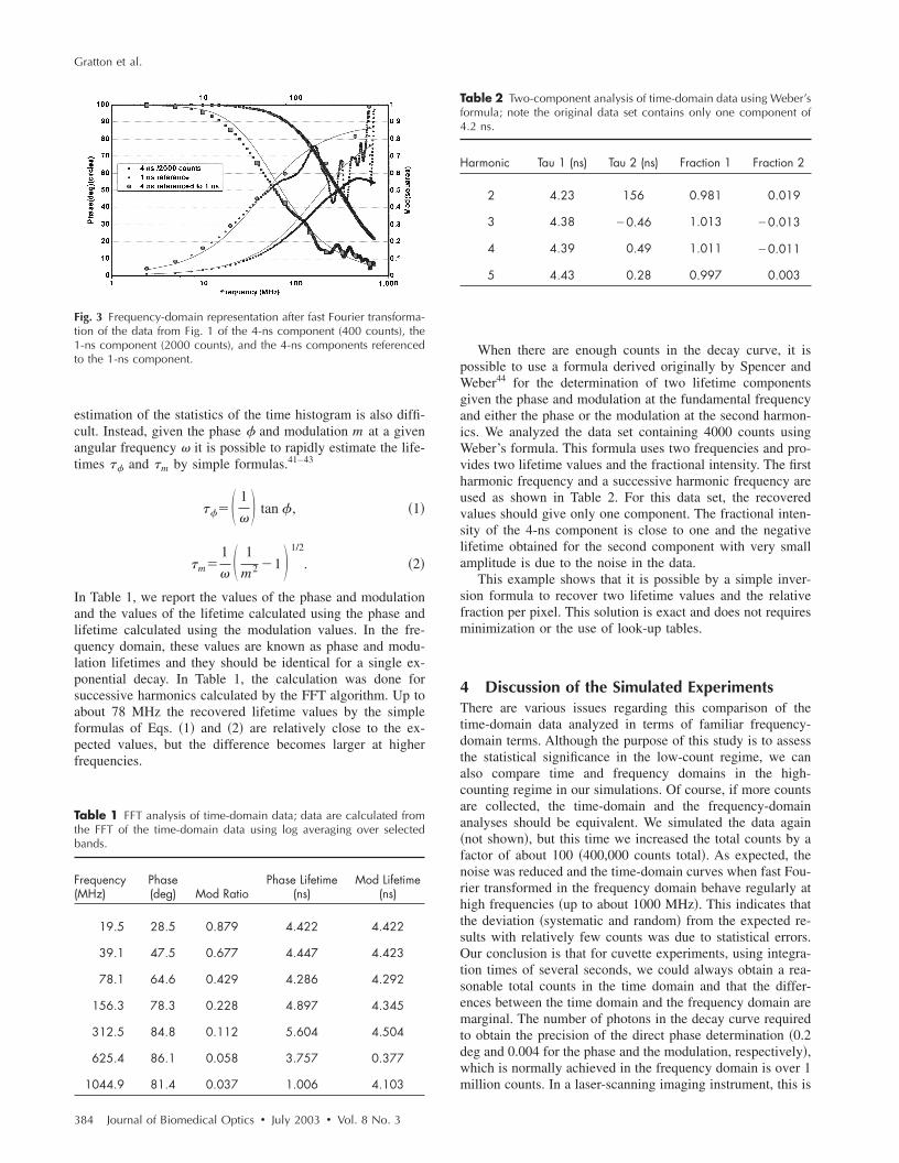
We repeated the simulation for a factor of 10 less countsfor the 4-ns sample �400 counts total�. The time-domain dataare shown in Fig. 1 and the time-domain data set after the FFTis shown in Fig. 3. For this count rate, the deviation from theexpected result �solid curve� is severe everywhere and par-ticularly over 100 MHz. This result is in agreement with ourestimation that no more that one or two harmonic frequenciescan be used for the determination of the lifetime in a pixel.

Next, we show that it is possible to calculate the lifetimevalue from the time-domain data using a very rapid procedurebased on exact frequency-domain formulas.

Although the fit of the decay in the time- and thefrequency-domains correctly recovers the lifetime values, theleast-squares procedure with lamp deconvolution used to re-cover the lifetime value is prohibitive in terms of computertime for the analysis of an image that contains of the order of105 pixels. Furthermore, when the counts are very low, the

Fig. 1 Simulated time-domain decay for 4-ns component (4000counts), 4-ns component (400 counts), and a reference compound of1 ns (2000 counts). The solid lines correspond to a fit using GlobalsWE software. The recovered lifetimes are reported in the text. Thelamp curve (not shown) has a width of 300 ps.

Fig. 2 Frequency-domain representation after fast Fourier transforma-tion of the data from Fig. 1 of the 4-ns component (4000 counts), the1-ns component (2000 counts), and the 4-ns components referencedto the 1-ns component.

Fluorescence lifetime imaging for the two-photon microscope . . .


estimation of the statistics of the time histogram is also diffi-cult. Instead, given the phase � and modulation m at a givenangular frequency � it is possible to rapidly estimate the life-times �� and �m by simple formulas.41–43

�� 1

� � tan � , �1�

�m�1

� � 1

m2 �1 � 1/2

. �2�

In Table 1, we report the values of the phase and modulationand the values of the lifetime calculated using the phase andlifetime calculated using the modulation values. In the fre-quency domain, these values are known as phase and modu-lation lifetimes and they should be identical for a single ex-ponential decay. In Table 1, the calculation was done forsuccessive harmonics calculated by the FFT algorithm. Up toabout 78 MHz the recovered lifetime values by the simpleformulas of Eqs. �1� and �2� are relatively close to the ex-pected values, but the difference becomes larger at higherfrequencies.

When there are enough counts in the decay curve, it ispossible to use a formula derived originally by Spencer andWeber44 for the determination of two lifetime componentsgiven the phase and modulation at the fundamental frequencyand either the phase or the modulation at the second harmon-ics. We analyzed the data set containing 4000 counts usingWeber’s formula. This formula uses two frequencies and pro-vides two lifetime values and the fractional intensity. The firstharmonic frequency and a successive harmonic frequency areused as shown in Table 2. For this data set, the recoveredvalues should give only one component. The fractional inten-sity of the 4-ns component is close to one and the negativelifetime obtained for the second component with very smallamplitude is due to the noise in the data.

This example shows that it is possible by a simple inver-sion formula to recover two lifetime values and the relativefraction per pixel. This solution is exact and does not requiresminimization or the use of look-up tables.

4 Discussion of the Simulated ExperimentsThere are various issues regarding this comparison of thetime-domain data analyzed in terms of familiar frequency-domain terms. Although the purpose of this study is to assessthe statistical significance in the low-count regime, we canalso compare time and frequency domains in the high-counting regime in our simulations. Of course, if more countsare collected, the time-domain and the frequency-domainanalyses should be equivalent. We simulated the data again�not shown�, but this time we increased the total counts by afactor of about 100 �400,000 counts total�. As expected, thenoise was reduced and the time-domain curves when fast Fou-rier transformed in the frequency domain behave regularly athigh frequencies �up to about 1000 MHz�. This indicates thatthe deviation �systematic and random� from the expected re-sults with relatively few counts was due to statistical errors.Our conclusion is that for cuvette experiments, using integra-tion times of several seconds, we could always obtain a rea-sonable total counts in the time domain and that the differ-ences between the time domain and the frequency domain aremarginal. The number of photons in the decay curve requiredto obtain the precision of the direct phase determination �0.2deg and 0.004 for the phase and the modulation, respectively�,which is normally achieved in the frequency domain is over 1million counts. In a laser-scanning imaging instrument, this is

Fig. 3 Frequency-domain representation after fast Fourier transforma-tion of the data from Fig. 1 of the 4-ns component (400 counts), the1-ns component (2000 counts), and the 4-ns components referencedto the 1-ns component.

Table 1 FFT analysis of time-domain data; data are calculated fromthe FFT of the time-domain data using log averaging over selectedbands.

Frequency(MHz)

Phase(deg) Mod Ratio

Phase Lifetime(ns)

Mod Lifetime(ns)

19.5 28.5 0.879 4.422 4.422

39.1 47.5 0.677 4.447 4.423

78.1 64.6 0.429 4.286 4.292

156.3 78.3 0.228 4.897 4.345

312.5 84.8 0.112 5.604 4.504

625.4 86.1 0.058 3.757 0.377

1044.9 81.4 0.037 1.006 4.103

Table 2 Two-component analysis of time-domain data using Weber’sformula; note the original data set contains only one component of4.2 ns.

Harmonic Tau 1 (ns) Tau 2 (ns) Fraction 1 Fraction 2

2 4.23 156 0.981 0.019

3 4.38 �0.46 1.013 �0.013

4 4.39 0.49 1.011 �0.011

5 4.43 0.28 0.997 0.003

Gratton et al.


unlikely to be achieved due to the limit of pixel dwell timeand the speed of data acquisition of the photon-counting de-tector.

Instead, in the low count regime, the total number ofcounts collected determines the frequency range that can beusefully employed. In practice, only a very restricted fre-quency range can be employed and for most applications inFLI, one or two frequencies �the fundamental laser repetitionfrequency and the second harmonic� are sufficient. The higherharmonics have a very large error.

5 Fluorescence Lifetime Imaging in theLaser-Scanning SystemAs we stated, for FLI the most important consideration is thenumber of counts that we can reasonably expect in 1 pixel. Anupper limit for integration in a pixel is determined by the timerequired to collect a frame. It is reasonable to integrate over apixel for about 100 to 200 �s, which corresponds to a framerate of about 6.5 to 13 s for a 256�256 image. In severalexperiments done with our acquisition card �model B&H630�, we were limited to sustained data acquisition rates ofabout 2 MHZ. Note that this average rate is also close to themaximum instantaneous rate. This is due to the dead time ofthe card, which is estimated to be about 150 ns and to otherlimiting factors due to data transfer.

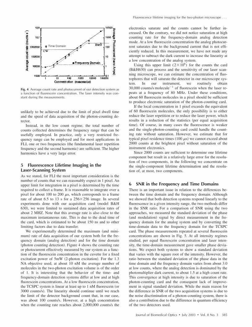
We experimentally determined the maximum �and mini-mum� rate of data acquisition of our system both for the fre-quency domain �analog detection� and for the time domain�photon counting detection�. Figure 4 shows the counting rateor photocurrent effectively measured by our system as a func-tion of the fluorescein concentration in the cuvette for a fixedexcitation power of 5mW �2-photon excitation�. For the 1.3NA objective used, at about 10 nM the average number ofmolecules in the two-photon excitation volume is of the orderof 1. It is interesting that the behavior of the time- andfrequency-domain detection systems differ at low and at highfluorescein concentrations. At a low fluorescein concentration,the TCSPC system is linear at least up to 1 nM fluorescein �or3000 counts/s�. The linearity should continue until we reachthe limit of the detector background count that, in our case,was about 100 counts/s. However, at a high concentrationwhen the counting rate reaches about 2,000,000 counts/s the

electronics saturate and the counts cannot be further in-creased. On the contrary, we did not notice saturation at highcounting rate for the frequency-domain analog detectionmode. At a low fluorescein concentration the analog photocur-rent saturates due to the background current that is not effi-ciently reduced. In this measurement, we have not made anyattempt to subtract the dark current to increase the linearity ata low concentration of the analog system.

Using this upper limit (2�106) for the counts the card�B&H630� can process and the sensitivity of our laser scan-ning microscope, we can estimate the concentration of fluo-rophores that will saturate the detector in our microscope sys-tem. In our instrument, we routinely obtain30,000 counts/s molecule�1 of fluorescein when the laser re-peats at a frequency of 80 MHz. Under these conditions,about 60 fluorescein molecules in a pixel should be sufficientto produce electronic saturation of the photon-counting card.

If the local concentration in 1 pixel exceeds the equivalentof 60 fluorescein molecules, the only possibility is to eitherreduce the laser repetition or to reduce the laser power, whichresults in a reduction of the statistics �per equal acquisitiontime�. Of course, in many cases the fluorescence is weakerand the single-photon-counting card could handle the count-ing rate without saturation. However, we estimate that fortypical pixel residence times �100 �s� we cannot exceed about2000 counts at the brightest pixel without saturation of theinstrument electronics.

Since 2000 counts are sufficient to determine one lifetimecomponent but result in a relatively large error for the resolu-tion of two components, in the following we concentrate onthe single-component lifetime determination and the resolu-tion of, at most, two components.

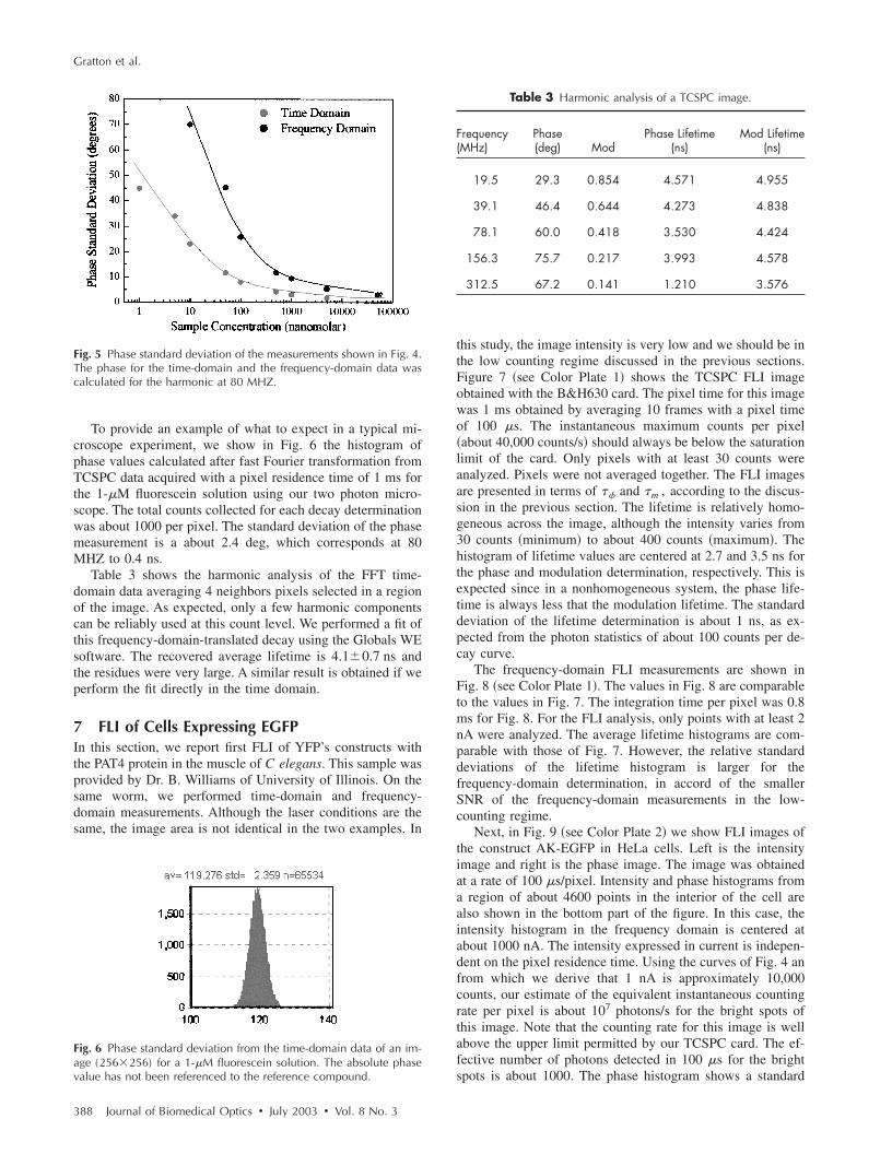
6 SNR in the Frequency and Time DomainsThere is an important issue in relation to the differences be-tween the time domain and the frequency domain. Althoughwe showed that both detection systems respond linearly to thefluorescence in a given intensity range, the two methods differin the SNR ratio. For a comparison of SNR using the twoapproaches, we measured the standard deviation of the phase�and modulation� signal by direct measurement in the fre-quency domain for the analog system and by converting thetime-domain data to the frequency domain for the TCSPCcard. The phase measurements repeated at several fluoresceinconcentrations are shown in Fig. 5. At all intensity regimesstudied, per equal fluorescein concentration and laser inten-sity, the time-domain measurement gave smaller phase devia-tions. We expect both systems to show a standard deviationthat varies with the square root of the intensity. However, theratio between the standard deviation of the phase data in thetime domain and the frequency domain varies from about 3.0at low counts, where the analog detection is dominated by thephotomultiplier dark current, to about 1.5 at a high count rate.This convergence at high intensity is due to saturation of thephoton-counting card and the consequent lack of improve-ment in signal standard deviation. While the main reason forthe difference in SNR of the two acquisition systems is due tothe noise discrimination of a photon-counting system, there isalso a contribution due to the difference in quantum efficiencyof the two detectors used.

Fig. 4 Average count rate and photocurrent of our detection system asa function of fluorescein concentration. The laser intensity was con-stant during the measurements.



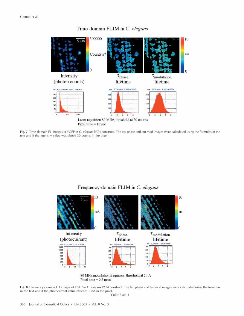
Fig. 7 Time-domain FLI images of YGFP in C. elegans PAT4 construct. The tau phase and tau mod images were calculated using the formulas in thetext and if the intensity value was above 30 counts in the pixel.

Fig. 8 Frequency-domain FLI images of YGFP in C. elegans PAT4 construct. The tau phase and tau mod images were calculated using the formulasin the text and if the photocurrent value exceeds 2 nA in the pixel.

Color Plate 1

Gratton et al.


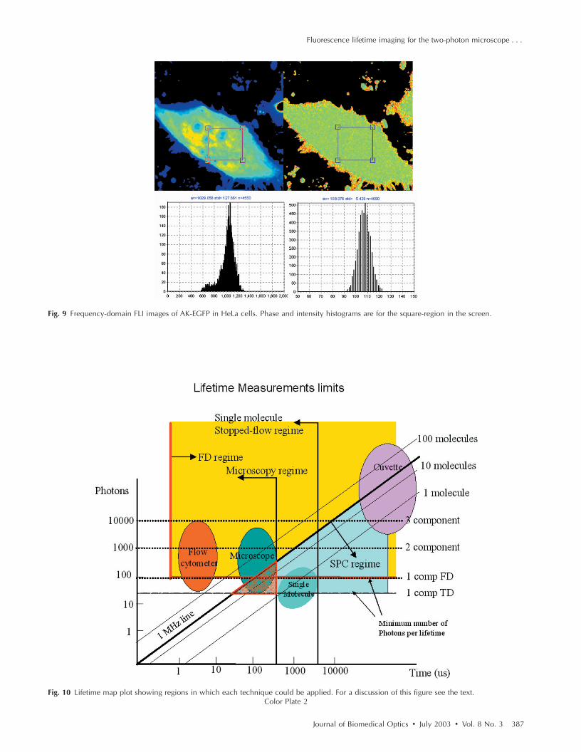
Fig. 9 Frequency-domain FLI images of AK-EGFP in HeLa cells. Phase and intensity histograms are for the square-region in the screen.

Fig. 10 Lifetime map plot showing regions in which each technique could be applied. For a discussion of this figure see the text.Color Plate 2



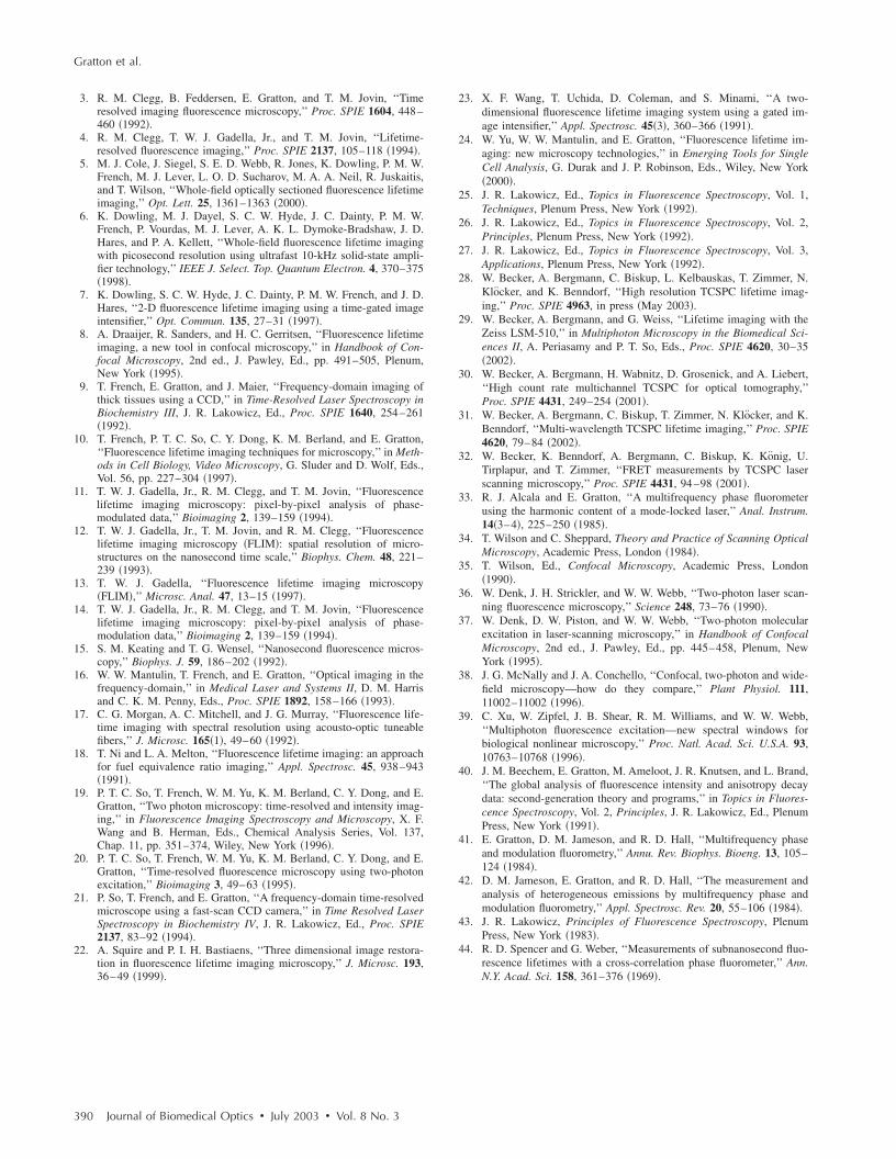
To provide an example of what to expect in a typical mi-croscope experiment, we show in Fig. 6 the histogram ofphase values calculated after fast Fourier transformation fromTCSPC data acquired with a pixel residence time of 1 ms forthe 1-�M fluorescein solution using our two photon micro-scope. The total counts collected for each decay determinationwas about 1000 per pixel. The standard deviation of the phasemeasurement is a about 2.4 deg, which corresponds at 80MHZ to 0.4 ns.

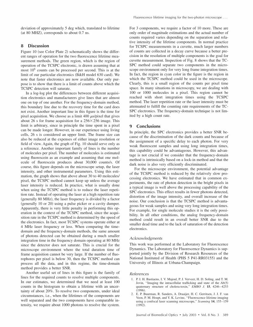
Table 3 shows the harmonic analysis of the FFT time-domain data averaging 4 neighbors pixels selected in a regionof the image. As expected, only a few harmonic componentscan be reliably used at this count level. We performed a fit ofthis frequency-domain-translated decay using the Globals WEsoftware. The recovered average lifetime is 4.1�0.7 ns andthe residues were very large. A similar result is obtained if weperform the fit directly in the time domain.

7 FLI of Cells Expressing EGFPIn this section, we report first FLI of YFP’s constructs withthe PAT4 protein in the muscle of C elegans. This sample wasprovided by Dr. B. Williams of University of Illinois. On thesame worm, we performed time-domain and frequency-domain measurements. Although the laser conditions are thesame, the image area is not identical in the two examples. In

this study, the image intensity is very low and we should be inthe low counting regime discussed in the previous sections.Figure 7 �see Color Plate 1� shows the TCSPC FLI imageobtained with the B&H630 card. The pixel time for this imagewas 1 ms obtained by averaging 10 frames with a pixel timeof 100 �s. The instantaneous maximum counts per pixel�about 40,000 counts/s� should always be below the saturationlimit of the card. Only pixels with at least 30 counts wereanalyzed. Pixels were not averaged together. The FLI imagesare presented in terms of �� and �m , according to the discus-sion in the previous section. The lifetime is relatively homo-geneous across the image, although the intensity varies from30 counts �minimum� to about 400 counts �maximum�. Thehistogram of lifetime values are centered at 2.7 and 3.5 ns forthe phase and modulation determination, respectively. This isexpected since in a nonhomogeneous system, the phase life-time is always less that the modulation lifetime. The standarddeviation of the lifetime determination is about 1 ns, as ex-pected from the photon statistics of about 100 counts per de-cay curve.

The frequency-domain FLI measurements are shown inFig. 8 �see Color Plate 1�. The values in Fig. 8 are comparableto the values in Fig. 7. The integration time per pixel was 0.8ms for Fig. 8. For the FLI analysis, only points with at least 2nA were analyzed. The average lifetime histograms are com-parable with those of Fig. 7. However, the relative standarddeviations of the lifetime histogram is larger for thefrequency-domain determination, in accord of the smallerSNR of the frequency-domain measurements in the low-counting regime.

Next, in Fig. 9 �see Color Plate 2� we show FLI images ofthe construct AK-EGFP in HeLa cells. Left is the intensityimage and right is the phase image. The image was obtainedat a rate of 100 �s/pixel. Intensity and phase histograms froma region of about 4600 points in the interior of the cell arealso shown in the bottom part of the figure. In this case, theintensity histogram in the frequency domain is centered atabout 1000 nA. The intensity expressed in current is indepen-dent on the pixel residence time. Using the curves of Fig. 4 anfrom which we derive that 1 nA is approximately 10,000counts, our estimate of the equivalent instantaneous countingrate per pixel is about 107 photons/s for the bright spots ofthis image. Note that the counting rate for this image is wellabove the upper limit permitted by our TCSPC card. The ef-fective number of photons detected in 100 �s for the brightspots is about 1000. The phase histogram shows a standard

Fig. 5 Phase standard deviation of the measurements shown in Fig. 4.The phase for the time-domain and the frequency-domain data wascalculated for the harmonic at 80 MHZ.

Fig. 6 Phase standard deviation from the time-domain data of an im-age (256�256) for a 1-�M fluorescein solution. The absolute phasevalue has not been referenced to the reference compound.

Table 3 Harmonic analysis of a TCSPC image.

Frequency(MHz)

Phase(deg) Mod

Phase Lifetime(ns)

Mod Lifetime(ns)

19.5 29.3 0.854 4.571 4.955

39.1 46.4 0.644 4.273 4.838

78.1 60.0 0.418 3.530 4.424

156.3 75.7 0.217 3.993 4.578

312.5 67.2 0.141 1.210 3.576

Gratton et al.


deviation of approximately 5 deg which, translated to lifetime�at 80 MHZ�, corresponds to about 0.7 ns.

8 DiscussionFigure 10 �see Color Plate 2� schematically shows the differ-ent ranges of operation for the two fluorescence lifetime mea-surement methods. The green region, which is the region ofoperation of the TCSPC electronic, is drawn assuming that atmost 106 counts can be processed per second. This is at thelimit of our particular electronics �B&H model 630 card�. Wenote that faster electronics are now available. Our only pur-pose is to show that there is a limit of counts above which theTCSPC detection will saturate.

In a log-log plot the differences between different acquisi-tion electronics and manufacturers give lines that are almostone on top of one another. For the frequency-domain method,this boundary line due to the recovery time for the card doesnot exist. Another important line in this figure is the time forpixel acquisition. We choose as a limit 400 �s/pixel that givesabout 26 s for frame acquisition for a 256�256 image. Thislimit is arbitrary, since in principle the time spent in a pixelcan be made longer. However, in our experience using livingcells, 26 s is considered an upper limit. The frame size canalso be reduced at the expenses of either image resolution orfield of view. Again, the graph of Fig. 10 should serve only asa reference. Another important family of lines is the numberof molecules per pixel. The number of molecules is estimatedusing fluorescein as an example and assuming that one mol-ecule of fluorescein produces about 30,000 counts/s. Ofcourse, this figure depends on the microscope setup, the laserintensity, and other instrumental parameters. Using this esti-mation, the graph shows that above about 30 to 40 molecules/pixel, the TCSPC method cannot keep up unless the averagelaser intensity is reduced. In practice, what is usually donewhen using the TCSPC method is to reduce the laser repeti-tion rate. Instead of operating the laser at a high repetition rate�generally 80 MHz�, the laser frequency is divided by a factor�generally 10 or 20� using a pulse picker or a cavity dumper.Apparently, there is very little penalty in performing this op-eration in the context of the TCSPC method, since the acqui-sition rate in the TCSPC method is determined by the speed ofthe electronics. In fact, most TCSPC systems operate either at4 MHz laser frequency or less. When comparing the time-domain and the frequency-domain methods, the same amountof photons detected can be obtained during a much smallerintegration time in the frequency domain operating at 80 MHzsince the detector does not saturate. This is crucial for themicroscope environment where the total duration time offrame acquisition cannot be very large. If the number of fluo-rophores per pixel is below 30, then the TCSPC method canprocess all the data, and in this regime, the time-domainmethod provides a better SNR.

Another useful set of lines in this figure is the family oflines for the required counts to resolve multiple components.In our estimates, we determined that we need at least 100counts in the histogram to obtain a lifetime with an uncer-tainty of about 20%. To resolve two components, under idealcircumstances, i.e., when the lifetimes of the components arewell separated and the two components have comparable in-tensity, we require about 1000 photons to resolve the system.

For 3 components, we require a factor of 10 more. These areonly order of magnitude estimations and the actual number ofcounts required varies depending on the separation and rela-tive intensity of the lifetime components. In normal practicefor TCSPC measurements in a cuvette, much larger numbersof counts are collected in a decay curve because a better pre-cision in the resolution of multiple components is the goal forcuvette measurement. Inspection of Fig. 8 shows that the TC-SPC method could separate two components in the micro-scope environment only for very long frame integration times.In fact, the region in cyan color in the figure is the region inwhich the TCSPC method could be used in the microscope.Clearly, this is a small region of the counts per pixel timespace. In many situations in microscopy, we are dealing with100 or 1000 molecules in a pixel. This region cannot bereached with short integration times using the TCSPCmethod. The laser repetition rate or the laser intensity must beattenuated to fulfill the counting rate requirements of the TC-SPC electronics. The frequency-domain technique is not lim-ited by a high count rate.

9 ConclusionsIn principle, the SPC electronics provides a better SNR be-cause of the discrimination of the dark counts and because ofthe assignment of a specific delay to each photon. For veryweak fluorescent samples and using long integration times,this capability could be advantageous. However, this advan-tage is not crucial if we consider that the frequency-domainmethod is intrinsically based on a lock-in method and that thedark noise is also very efficiently discriminated.

For the microscope environment, the potential advantageof the TCSPC method is reduced by the relatively slow pro-cessing electronics. We have estimated that in common ex-periments, the rate of photon detection in the bright pixels ina typical image is well above the processing capability of theSPC electronics. This effect results in fewer photons detected,distortion of the image intensity, and overall increase of thenoise. Our conclusion is that the TCSPC method is advanta-geous for weak samples and using very long integration times.For example, for single molecule studies it is the only possi-bility. In all other conditions, the analog frequency-domainmethod could result in an overall better SNR due to thesmaller dead time and to the lack of saturation of the detectionelectronics.

AcknowledgmentsThis work was performed at the Laboratory for FluorescenceDynamics. The Laboratory for Fluorescence Dynamics is sup-ported jointly by the Division of Research Resources of theNational Instituted of Health �PHS 5 P41-RR03155� and theUniversity of Illinois at Urbana-Champaign.

References1. P. I. H. Bastiaens, I. V. Majoul, P. J. Verveer, H. D. Soling, and T. M.

Jovin, ‘‘Imaging the intracellular trafficking and state of the Ab�5�quaternary structure of cholera-toxin,’’ EMBO J. 15, 4246–4253�1996�.

2. E. P. Buurman, R. Sanders, A. Draaijer, H. C. Gerritsen, J. J. F. vanVeen, P. M. Houpt, and Y. K. Levine, ‘‘Fluorescence lifetime imagingusing a confocal laser scanning microscope,’’ Scanning 14, 155–159�1992�.



3. R. M. Clegg, B. Feddersen, E. Gratton, and T. M. Jovin, ‘‘Timeresolved imaging fluorescence microscopy,’’ Proc. SPIE 1604, 448–460 �1992�.

4. R. M. Clegg, T. W. J. Gadella, Jr., and T. M. Jovin, ‘‘Lifetime-resolved fluorescence imaging,’’ Proc. SPIE 2137, 105–118 �1994�.

5. M. J. Cole, J. Siegel, S. E. D. Webb, R. Jones, K. Dowling, P. M. W.French, M. J. Lever, L. O. D. Sucharov, M. A. A. Neil, R. Juskaitis,and T. Wilson, ‘‘Whole-field optically sectioned fluorescence lifetimeimaging,’’ Opt. Lett. 25, 1361–1363 �2000�.

6. K. Dowling, M. J. Dayel, S. C. W. Hyde, J. C. Dainty, P. M. W.French, P. Vourdas, M. J. Lever, A. K. L. Dymoke-Bradshaw, J. D.Hares, and P. A. Kellett, ‘‘Whole-field fluorescence lifetime imagingwith picosecond resolution using ultrafast 10-kHz solid-state ampli-fier technology,’’ IEEE J. Select. Top. Quantum Electron. 4, 370–375�1998�.

7. K. Dowling, S. C. W. Hyde, J. C. Dainty, P. M. W. French, and J. D.Hares, ‘‘2-D fluorescence lifetime imaging using a time-gated imageintensifier,’’ Opt. Commun. 135, 27–31 �1997�.

8. A. Draaijer, R. Sanders, and H. C. Gerritsen, ‘‘Fluorescence lifetimeimaging, a new tool in confocal microscopy,’’ in Handbook of Con-focal Microscopy, 2nd ed., J. Pawley, Ed., pp. 491–505, Plenum,New York �1995�.

9. T. French, E. Gratton, and J. Maier, ‘‘Frequency-domain imaging ofthick tissues using a CCD,’’ in Time-Resolved Laser Spectroscopy inBiochemistry III, J. R. Lakowicz, Ed., Proc. SPIE 1640, 254–261�1992�.

10. T. French, P. T. C. So, C. Y. Dong, K. M. Berland, and E. Gratton,‘‘Fluorescence lifetime imaging techniques for microscopy,’’ in Meth-ods in Cell Biology, Video Microscopy, G. Sluder and D. Wolf, Eds.,Vol. 56, pp. 227–304 �1997�.

11. T. W. J. Gadella, Jr., R. M. Clegg, and T. M. Jovin, ‘‘Fluorescencelifetime imaging microscopy: pixel-by-pixel analysis of phase-modulated data,’’ Bioimaging 2, 139–159 �1994�.

12. T. W. J. Gadella, Jr., T. M. Jovin, and R. M. Clegg, ‘‘Fluorescencelifetime imaging microscopy �FLIM�: spatial resolution of micro-structures on the nanosecond time scale,’’ Biophys. Chem. 48, 221–239 �1993�.

13. T. W. J. Gadella, ‘‘Fluorescence lifetime imaging microscopy�FLIM�,’’ Microsc. Anal. 47, 13–15 �1997�.

14. T. W. J. Gadella, Jr., R. M. Clegg, and T. M. Jovin, ‘‘Fluorescencelifetime imaging microscopy: pixel-by-pixel analysis of phase-modulation data,’’ Bioimaging 2, 139–159 �1994�.

15. S. M. Keating and T. G. Wensel, ‘‘Nanosecond fluorescence micros-copy,’’ Biophys. J. 59, 186–202 �1992�.

16. W. W. Mantulin, T. French, and E. Gratton, ‘‘Optical imaging in thefrequency-domain,’’ in Medical Laser and Systems II, D. M. Harrisand C. K. M. Penny, Eds., Proc. SPIE 1892, 158–166 �1993�.

17. C. G. Morgan, A. C. Mitchell, and J. G. Murray, ‘‘Fluorescence life-time imaging with spectral resolution using acousto-optic tuneablefibers,’’ J. Microsc. 165�1�, 49–60 �1992�.

18. T. Ni and L. A. Melton, ‘‘Fluorescence lifetime imaging: an approachfor fuel equivalence ratio imaging,’’ Appl. Spectrosc. 45, 938–943�1991�.

19. P. T. C. So, T. French, W. M. Yu, K. M. Berland, C. Y. Dong, and E.Gratton, ‘‘Two photon microscopy: time-resolved and intensity imag-ing,’’ in Fluorescence Imaging Spectroscopy and Microscopy, X. F.Wang and B. Herman, Eds., Chemical Analysis Series, Vol. 137,Chap. 11, pp. 351–374, Wiley, New York �1996�.

20. P. T. C. So, T. French, W. M. Yu, K. M. Berland, C. Y. Dong, and E.Gratton, ‘‘Time-resolved fluorescence microscopy using two-photonexcitation,’’ Bioimaging 3, 49–63 �1995�.

21. P. So, T. French, and E. Gratton, ‘‘A frequency-domain time-resolvedmicroscope using a fast-scan CCD camera,’’ in Time Resolved LaserSpectroscopy in Biochemistry IV, J. R. Lakowicz, Ed., Proc. SPIE2137, 83–92 �1994�.

22. A. Squire and P. I. H. Bastiaens, ‘‘Three dimensional image restora-tion in fluorescence lifetime imaging microscopy,’’ J. Microsc. 193,36–49 �1999�.

23. X. F. Wang, T. Uchida, D. Coleman, and S. Minami, ‘‘A two-dimensional fluorescence lifetime imaging system using a gated im-age intensifier,’’ Appl. Spectrosc. 45�3�, 360–366 �1991�.

24. W. Yu, W. W. Mantulin, and E. Gratton, ‘‘Fluorescence lifetime im-aging: new microscopy technologies,’’ in Emerging Tools for SingleCell Analysis, G. Durak and J. P. Robinson, Eds., Wiley, New York�2000�.

25. J. R. Lakowicz, Ed., Topics in Fluorescence Spectroscopy, Vol. 1,Techniques, Plenum Press, New York �1992�.

26. J. R. Lakowicz, Ed., Topics in Fluorescence Spectroscopy, Vol. 2,Principles, Plenum Press, New York �1992�.

27. J. R. Lakowicz, Ed., Topics in Fluorescence Spectroscopy, Vol. 3,Applications, Plenum Press, New York �1992�.

28. W. Becker, A. Bergmann, C. Biskup, L. Kelbauskas, T. Zimmer, N.Klocker, and K. Benndorf, ‘‘High resolution TCSPC lifetime imag-ing,’’ Proc. SPIE 4963, in press �May 2003�.

29. W. Becker, A. Bergmann, and G. Weiss, ‘‘Lifetime imaging with theZeiss LSM-510,’’ in Multiphoton Microscopy in the Biomedical Sci-ences II, A. Periasamy and P. T. So, Eds., Proc. SPIE 4620, 30–35�2002�.

30. W. Becker, A. Bergmann, H. Wabnitz, D. Grosenick, and A. Liebert,‘‘High count rate multichannel TCSPC for optical tomography,’’Proc. SPIE 4431, 249–254 �2001�.

31. W. Becker, A. Bergmann, C. Biskup, T. Zimmer, N. Klocker, and K.Benndorf, ‘‘Multi-wavelength TCSPC lifetime imaging,’’ Proc. SPIE4620, 79–84 �2002�.

32. W. Becker, K. Benndorf, A. Bergmann, C. Biskup, K. Konig, U.Tirplapur, and T. Zimmer, ‘‘FRET measurements by TCSPC laserscanning microscopy,’’ Proc. SPIE 4431, 94–98 �2001�.

33. R. J. Alcala and E. Gratton, ‘‘A multifrequency phase fluorometerusing the harmonic content of a mode-locked laser,’’ Anal. Instrum.14�3–4�, 225–250 �1985�.

34. T. Wilson and C. Sheppard, Theory and Practice of Scanning OpticalMicroscopy, Academic Press, London �1984�.

35. T. Wilson, Ed., Confocal Microscopy, Academic Press, London�1990�.

36. W. Denk, J. H. Strickler, and W. W. Webb, ‘‘Two-photon laser scan-ning fluorescence microscopy,’’ Science 248, 73–76 �1990�.

37. W. Denk, D. W. Piston, and W. W. Webb, ‘‘Two-photon molecularexcitation in laser-scanning microscopy,’’ in Handbook of ConfocalMicroscopy, 2nd ed., J. Pawley, Ed., pp. 445–458, Plenum, NewYork �1995�.

38. J. G. McNally and J. A. Conchello, ‘‘Confocal, two-photon and wide-field microscopy—how do they compare,’’ Plant Physiol. 111,11002–11002 �1996�.

39. C. Xu, W. Zipfel, J. B. Shear, R. M. Williams, and W. W. Webb,‘‘Multiphoton fluorescence excitation—new spectral windows forbiological nonlinear microscopy,’’ Proc. Natl. Acad. Sci. U.S.A. 93,10763–10768 �1996�.

40. J. M. Beechem, E. Gratton, M. Ameloot, J. R. Knutsen, and L. Brand,‘‘The global analysis of fluorescence intensity and anisotropy decaydata: second-generation theory and programs,’’ in Topics in Fluores-cence Spectroscopy, Vol. 2, Principles, J. R. Lakowicz, Ed., PlenumPress, New York �1991�.

41. E. Gratton, D. M. Jameson, and R. D. Hall, ‘‘Multifrequency phaseand modulation fluorometry,’’ Annu. Rev. Biophys. Bioeng. 13, 105–124 �1984�.

42. D. M. Jameson, E. Gratton, and R. D. Hall, ‘‘The measurement andanalysis of heterogeneous emissions by multifrequency phase andmodulation fluorometry,’’ Appl. Spectrosc. Rev. 20, 55–106 �1984�.

43. J. R. Lakowicz, Principles of Fluorescence Spectroscopy, PlenumPress, New York �1983�.

44. R. D. Spencer and G. Weber, ‘‘Measurements of subnanosecond fluo-rescence lifetimes with a cross-correlation phase fluorometer,’’ Ann.N.Y. Acad. Sci. 158, 361–376 �1969�.

Gratton et al.


Documents

Fluorescence lifetime imaging for the two-photon ... · Fluorescence lifetime imaging for the two-photon microscope: time-domain and frequency-domain methods ... Journal of Biomedical