FluxSimulator: An R Package to Simulate Isotopomer

JSS Journal of Statistical SoftwareJanuary 2007, Volume 18, Issue 7. http://www.jstatsoft.org/

FluxSimulator: An R Package to Simulate

Isotopomer Distributions in Metabolic Networks

Thomas W. BinslVrije Universiteit Amsterdam

Katharine M. MullenVrije Universiteit Amsterdam

Ivo H. M. van StokkumVrije Universiteit Amsterdam

Jaap HeringaVrije Universiteit Amsterdam

Johannes H. G. M. van BeekVrije Universiteit Medical Centre Amsterdam

Abstract

The representation of biochemical knowledge in terms of fluxes (transformation rates)in a metabolic network is often a crucial step in the development of new drugs and effi-cient bioreactors. Mass spectroscopy (MS) and nuclear magnetic resonance spectroscopy(NMRS) in combination with 13C labeled substrates are experimental techniques resultingin data that may be used to quantify fluxes in the metabolic network underlying a process.The massive amount of data generated by spectroscopic experiments increasingly requiressoftware which models the dynamics of the underlying biological system.

In this work we present an approach to handle isotopomer distributions in metabolicnetworks using an object-oriented programming approach, implemented using S4 classesin R. The developed package is called FluxSimulator and provides a user friendly inter-face to specify the topological information of the metabolic network as well as carbonatom transitions in plain text files. The package automatically derives the mathemati-cal representation of the formulated network, and assembles a set of ordinary differentialequations (ODEs) describing the change of each isotopomer pool over time. These ODEsare subsequently solved numerically.

In a case study FluxSimulator was applied to an example network. Our results indicatethat the package is able to reproduce exact changes in isotopomer compositions of themetabolite pools over time at given flux rates.

Keywords: metabolism, flux, isotopomer labeling, ODE, R, MS, NMRS, systems biology.

http://www.jstatsoft.org/

2 FluxSimulator: Simulation of Isotopomer Distributions in Metabolic Networks in R

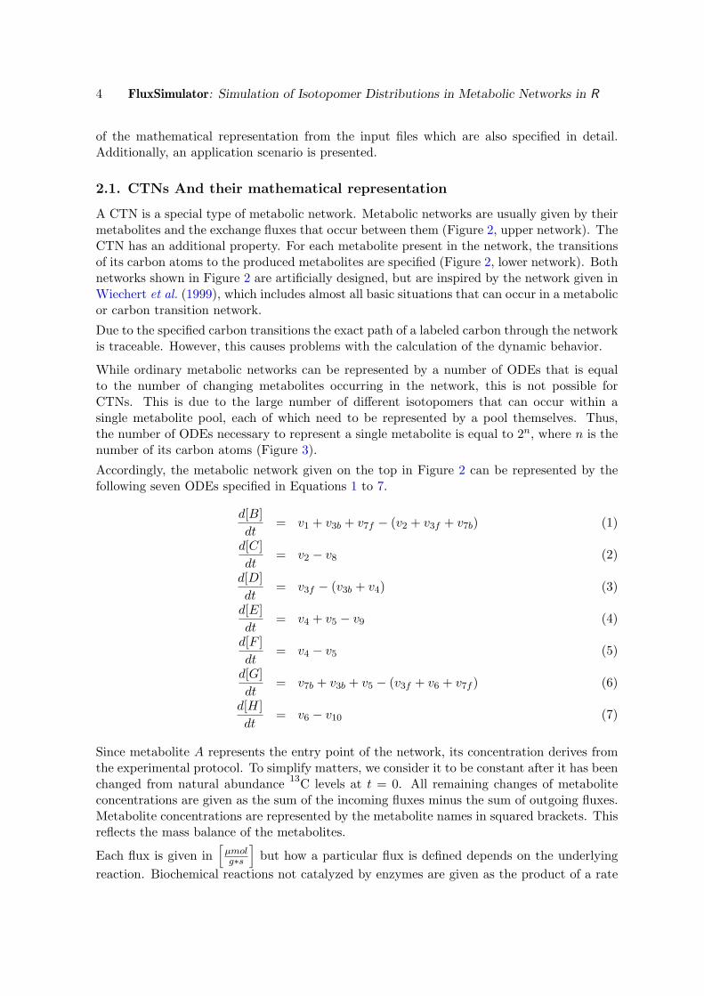
1. Introduction

Dedicated drug development (Bohm et al. 2002; Leach and Gillet 2003) and the design ofnew efficient bioreactors (Dunn et al. 2003) is a great challenge for the pharmaceutical andbiotechnological industries. Progress often depends on the exact knowledge of biochemicalreactions between chemical compounds. As these reactions occur in the metabolism of patientsor microorganisms the reactions are termed metabolic reactions and the chemical compoundsmetabolites. Both can be represented via so called metabolic network models which allow fortheir quantitative investigation. We will provide two case scenarios to highlight this, basedon the small sample network given in Figure 1.

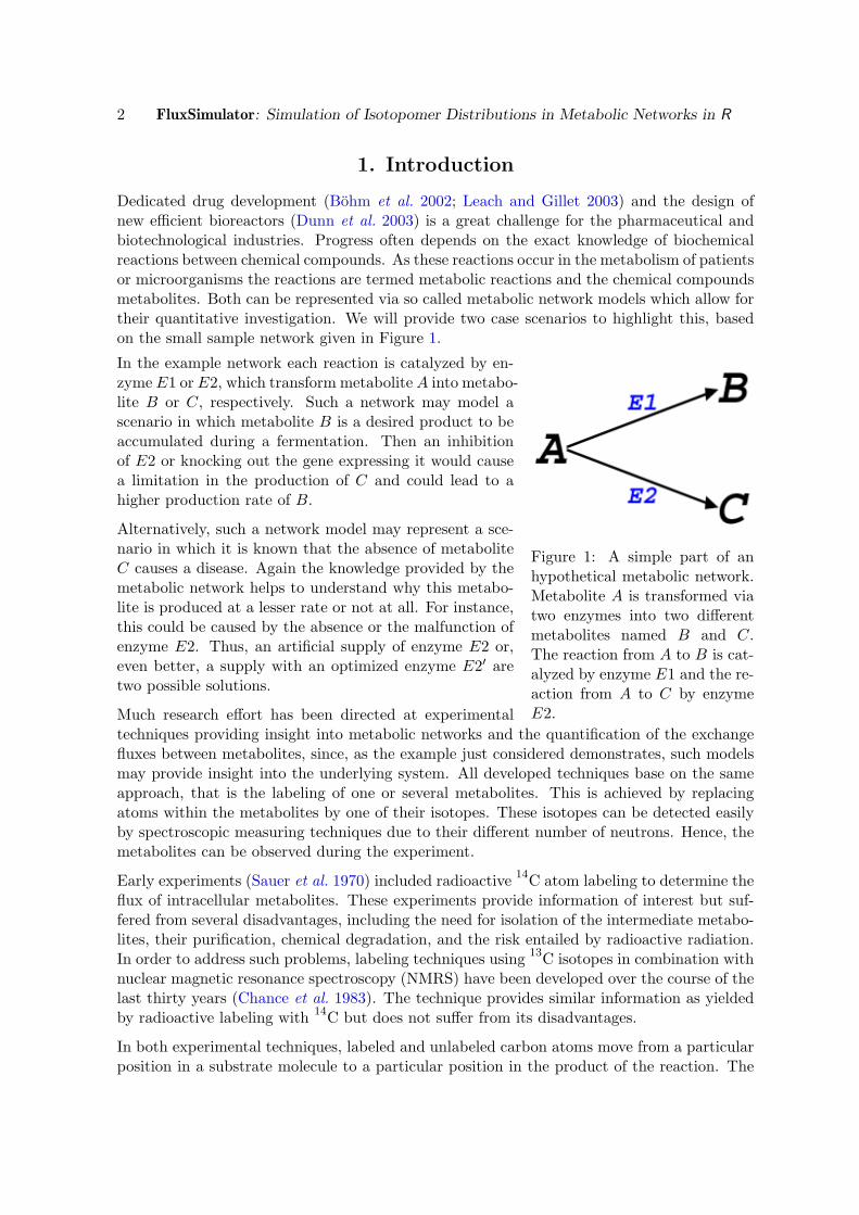
In the example network each reaction is catalyzed by en-

Figure 1: A simple part of anhypothetical metabolic network.Metabolite A is transformed viatwo enzymes into two differentmetabolites named B and C.The reaction from A to B is cat-alyzed by enzyme E1 and the re-action from A to C by enzymeE2.

zyme E1 or E2, which transform metabolite A into metabo-lite B or C, respectively. Such a network may model ascenario in which metabolite B is a desired product to beaccumulated during a fermentation. Then an inhibitionof E2 or knocking out the gene expressing it would causea limitation in the production of C and could lead to ahigher production rate of B.

Alternatively, such a network model may represent a sce-nario in which it is known that the absence of metaboliteC causes a disease. Again the knowledge provided by themetabolic network helps to understand why this metabo-lite is produced at a lesser rate or not at all. For instance,this could be caused by the absence or the malfunction ofenzyme E2. Thus, an artificial supply of enzyme E2 or,even better, a supply with an optimized enzyme E2′ aretwo possible solutions.

Much research effort has been directed at experimentaltechniques providing insight into metabolic networks and the quantification of the exchangefluxes between metabolites, since, as the example just considered demonstrates, such modelsmay provide insight into the underlying system. All developed techniques base on the sameapproach, that is the labeling of one or several metabolites. This is achieved by replacingatoms within the metabolites by one of their isotopes. These isotopes can be detected easilyby spectroscopic measuring techniques due to their different number of neutrons. Hence, themetabolites can be observed during the experiment.

Early experiments (Sauer et al. 1970) included radioactive 14C atom labeling to determine theflux of intracellular metabolites. These experiments provide information of interest but suf-fered from several disadvantages, including the need for isolation of the intermediate metabo-lites, their purification, chemical degradation, and the risk entailed by radioactive radiation.In order to address such problems, labeling techniques using 13C isotopes in combination withnuclear magnetic resonance spectroscopy (NMRS) have been developed over the course of thelast thirty years (Chance et al. 1983). The technique provides similar information as yieldedby radioactive labeling with 14C but does not suffer from its disadvantages.

In both experimental techniques, labeled and unlabeled carbon atoms move from a particularposition in a substrate molecule to a particular position in the product of the reaction. The

Journal of Statistical Software 3

set of all transitions between carbon atoms in substrates and products is termed the carbontransition network (CTN). Metabolic networks consists of several metabolite pools, where eachparticular pool is the sum of all metabolites belonging to the same chemical species. Withina carbon transition network these pools are additionally subdivided into particular fractions.This is due to the 2n different labeling states that can occur in a metabolite consisting of ncarbons. Each of these labeling states is termed an isotopomer and forms a subpool withinits particular metabolite pool.

Hence, to analyze 13C NMRS experiments, software to simulate and interpret these carbontransition networks is necessary. Several approaches have been implemented previously. Forinstance, van Beek et al. (1998) and van Beek et al. (1999), developed and implementedcomputer programs in FORTRAN to simulate the dynamics of various metabolic networkmodels. Such FORTRAN programs achieve accurate simulation results but suffer from limitedflexibility and are error-prone during the manual implementation of the ODEs. This is due tothe fact that each model has to be hard coded in a subroutine, which is linked to a simulationcomputer program.

Another approach is using existing software packages like Berkeley Madonna (Macey et al.2000) or JSIM (Raymond et al. 2003) to simulate dynamic systems. Here again, the programsrequire hard-coding of the model in a specially defined mathematical language.

Yet another approach by Wiechert et al. (1995); Wiechert and de Graaf (1997); Wiechertet al. (1997, 1999); Wiechert (2001) consists of the algorithms to analyze and simulate 13Clabeling experiments. Wiechert et al. (2001) incorporated these developments into a softwarepackage (Wiechert et al. 2001).

This package considers the underlying network to be in metabolic and isotopomeric steadystate, i.e., it assumes that the concentrations of the particular metabolites and their iso-topomers do not change over time. As new experimental approaches go beyond these as-sumptions, programs must be developed to handle non-steady state systems. Furthermore,the package is written in C++ and must be used on a Linux platform.

To address the above limitations we have developed a package in the high level languageR (R Development Core Team 2006). The package is designed to simulate the carbon atomtransitions occurring in a metabolic network (Carbon Transition Network, CTN) over time. Inaddition to algorithms solving ODEs efficiently, R provides features for parameter estimationand statistics that will facilitate the extension of the package in the future. Furthermore, Ris cross-platform and can be run on all major operating systems like Linux, Windows andMacOS. The developed R package is called FluxSimulator and can be used without any skillsin programming or handling ordinary differential equations (ODEs).

An example of a CTN, its mathematical representation, the derivation from the input filesas well as an exact specification of the input files is given in the Section 2. Additionally, weperformed an example simulation and compared the results to a simulation done with BerkeleyMadonna. This comparison is analyzed and discussed in Section 3. Final conclusions and anoutlook to future work are given in Section 4.

2. Methods

This section introduces an example CTN. It is used to explain the automatic derivation


of the mathematical representation from the input files which are also specified in detail.Additionally, an application scenario is presented.

2.1. CTNs And their mathematical representation

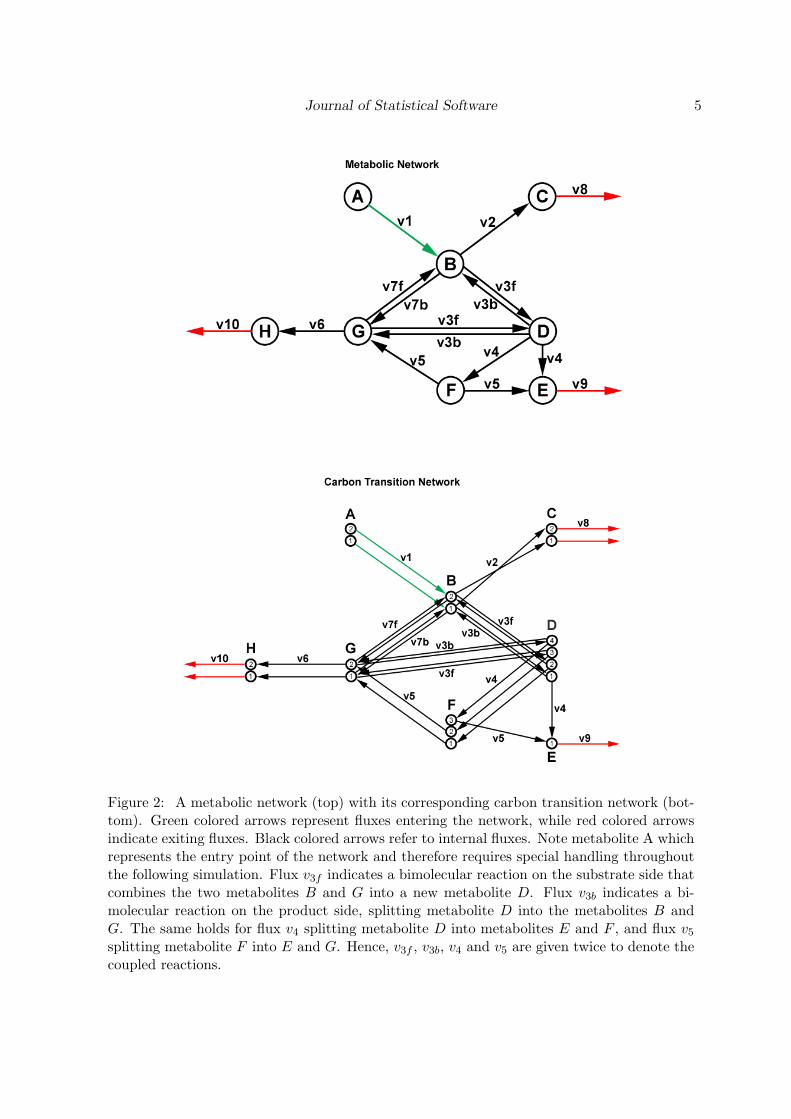
A CTN is a special type of metabolic network. Metabolic networks are usually given by theirmetabolites and the exchange fluxes that occur between them (Figure 2, upper network). TheCTN has an additional property. For each metabolite present in the network, the transitionsof its carbon atoms to the produced metabolites are specified (Figure 2, lower network). Bothnetworks shown in Figure 2 are artificially designed, but are inspired by the network given inWiechert et al. (1999), which includes almost all basic situations that can occur in a metabolicor carbon transition network.

Due to the specified carbon transitions the exact path of a labeled carbon through the networkis traceable. However, this causes problems with the calculation of the dynamic behavior.

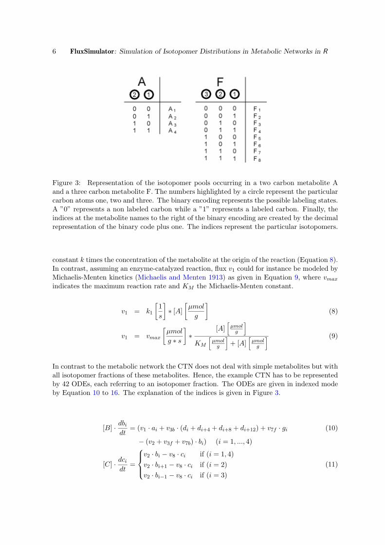
While ordinary metabolic networks can be represented by a number of ODEs that is equalto the number of changing metabolites occurring in the network, this is not possible forCTNs. This is due to the large number of different isotopomers that can occur within asingle metabolite pool, each of which need to be represented by a pool themselves. Thus,the number of ODEs necessary to represent a single metabolite is equal to 2n, where n is thenumber of its carbon atoms (Figure 3).

Accordingly, the metabolic network given on the top in Figure 2 can be represented by thefollowing seven ODEs specified in Equations 1 to 7.

d[B]dt

= v1 + v3b + v7f − (v2 + v3f + v7b) (1)

d[C]dt

= v2 − v8 (2)

d[D]dt

= v3f − (v3b + v4) (3)

d[E]dt

= v4 + v5 − v9 (4)

d[F ]dt

= v4 − v5 (5)

d[G]dt

= v7b + v3b + v5 − (v3f + v6 + v7f ) (6)

d[H]dt

= v6 − v10 (7)

Since metabolite A represents the entry point of the network, its concentration derives fromthe experimental protocol. To simplify matters, we consider it to be constant after it has beenchanged from natural abundance 13C levels at t = 0. All remaining changes of metaboliteconcentrations are given as the sum of the incoming fluxes minus the sum of outgoing fluxes.Metabolite concentrations are represented by the metabolite names in squared brackets. Thisreflects the mass balance of the metabolites.

Each flux is given in[

µmolg∗s

]but how a particular flux is defined depends on the underlying

reaction. Biochemical reactions not catalyzed by enzymes are given as the product of a rate


Figure 2: A metabolic network (top) with its corresponding carbon transition network (bot-tom). Green colored arrows represent fluxes entering the network, while red colored arrowsindicate exiting fluxes. Black colored arrows refer to internal fluxes. Note metabolite A whichrepresents the entry point of the network and therefore requires special handling throughoutthe following simulation. Flux v3f indicates a bimolecular reaction on the substrate side thatcombines the two metabolites B and G into a new metabolite D. Flux v3b indicates a bi-molecular reaction on the product side, splitting metabolite D into the metabolites B andG. The same holds for flux v4 splitting metabolite D into metabolites E and F , and flux v5

splitting metabolite F into E and G. Hence, v3f , v3b, v4 and v5 are given twice to denote thecoupled reactions.


Figure 3: Representation of the isotopomer pools occurring in a two carbon metabolite Aand a three carbon metabolite F. The numbers highlighted by a circle represent the particularcarbon atoms one, two and three. The binary encoding represents the possible labeling states.A ”0” represents a non labeled carbon while a ”1” represents a labeled carbon. Finally, theindices at the metabolite names to the right of the binary encoding are created by the decimalrepresentation of the binary code plus one. The indices represent the particular isotopomers.

constant k times the concentration of the metabolite at the origin of the reaction (Equation 8).In contrast, assuming an enzyme-catalyzed reaction, flux v1 could for instance be modeled byMichaelis-Menten kinetics (Michaelis and Menten 1913) as given in Equation 9, where vmax

indicates the maximum reaction rate and KM the Michaelis-Menten constant.

v1 = k1

[1s

]∗ [A]

[µmol

g

](8)

v1 = vmax

[µmol

g ∗ s

]∗

[A][

µmolg

]KM

[µmol

g

]+ [A]

[µmol

g

] (9)

In contrast to the metabolic network the CTN does not deal with simple metabolites but withall isotopomer fractions of these metabolites. Hence, the example CTN has to be representedby 42 ODEs, each referring to an isotopomer fraction. The ODEs are given in indexed modeby Equation 10 to 16. The explanation of the indices is given in Figure 3.

[B] · dbi

dt= (v1 · ai + v3b · (di + di+4 + di+8 + di+12) + v7f · gi (10)

− (v2 + v3f + v7b) · bi) (i = 1, ..., 4)

[C] · dci

dt=

v2 · bi − v8 · ci if (i = 1, 4)v2 · bi+1 − v8 · ci if (i = 2)v2 · bi−1 − v8 · ci if (i = 3)

(11)


[D] · ddi

dt=

(v3f · bi · g1 − (v3b + v4) · di) if (i = 1, ..., 4)(v3f · bi−4 · g2 − (v3b + v4) · di) if (i = 5, ..., 8)(v3f · bi−8 · g3 − (v3b + v4) · di) if (i = 9, ..., 12)(v3f · bi−12 · g4 − (v3b + v4) · di) if (i = 13, ..., 16)

(12)

[E] · dei

dt=

(v4 ·

8∑j=1

d2j−1 + v5 ·4∑

j=1fj − v9 · ei) if (i = 1)

(v4 ·8∑

j=1d2j + v5 ·

8∑j=4

fj − v9 · ei) if (i = 2)(13)

[F ] · dfi

dt= (v4 ·

2i∑j=2i−1

dj − v5 · fi) (i = 1, ..., 8) (14)

[G] · dgi

dt=

(v7b · bi +4∑

j=1v3b · dj + v5 · (fi + fi+4)

−(v3f + v6 + v7f ) · gi) if (i = 1)

(v7b · bi +8∑

j=5v3b · dj + v5 · (fi + fi+4)

−(v3f + v6 + v7f ) · gi) if (i = 2)

(v7b · bi +12∑

j=9v3b · dj + v5 · (fi + fi+4)

−(v3f + v6 + v7f ) · gi) if (i = 3)

(v7b · bi +16∑

j=13v3b · dj + v5 · (fi + fi+4)

−(v3f + v6 + v7f ) · gi) if (i = 4)

(15)

[H] · dhi

dt= (v6 · gi − v10 · hi) (i = 1, ..., 4) (16)

Each isotopomer fraction is represented by the metabolite name in lower case letter combinedwith an index, e.g. di or dei. This index corresponds to the carbon atoms labeled in theparticular isotopomer fraction (see explanation in Figure 3). The fluxes are equal to thoseused in the previous Equations 1 to 7. From Equations 10 to 16 one can see that the timescale of change of the isotopomer fractions can be derived by dividing the incoming fluxes andoutgoing fluxes (right side of the equations) by the concentration of the receiving metabolitepool (concentration on the left side of the equations). As metabolite A is the entry of thenetwork its isotopomers are prescribed and are again not considered in the equations above.

With large numbers of ODEs two problems occur. The first problem is the increased chanceof possible mistakes in the ODEs if they have to be hard coded in the computer program.This is clearly illustrated by the complexity of the previous equations. An example for suchan encoding is given in the by the input file used for Berkeley Madonna which is availabletogether with the paper. The second problem is the increasing computational power necessaryto solve the ODEs numerically. To address the first problem, FluxSimulator is designed toderive the ODEs automatically from three simple text files described in Section 2.3.


2.2. Core algorithm

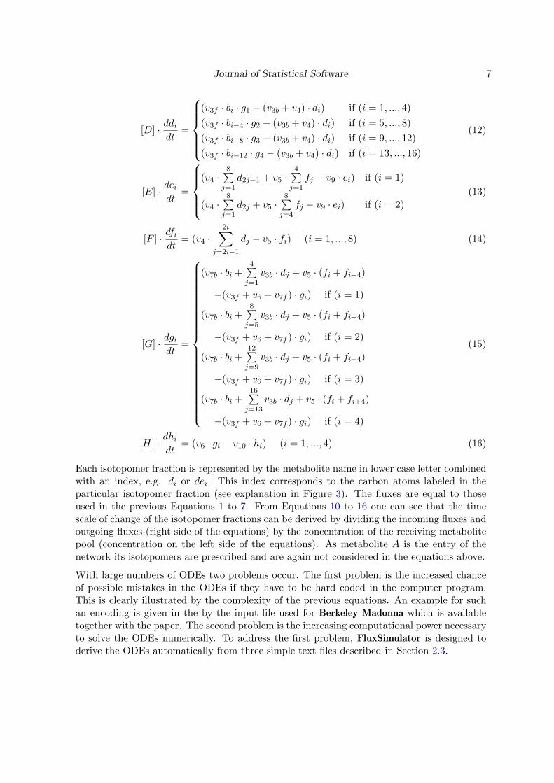
Initially, all input files are parsed and the data structures necessary to represent the CTNare constructed within the R environment. Afterwards, all ODEs representing the dynamicbehavior of the CTN are automatically derived, as illustrated in the subsequent flowchart inNassi-Shneiderman style (Nassi and Shneiderman 1973).

Core Algorithm — Deriving ODEs From Input Data

NOT ALL METABOLIC POOLS CONSIDERED

GET NEXT METABOLIC POOL

NOT ALL ISOTOPOMERS CONSIDERED

GET NEXT ISOTOPOMER

NOT ALL INFLUXES CONSIDERED

GET NEXT INFLUX

ZZ

ZY MULTIMOLECULAR REACTION�

��N

COMPUTE MULTIMOLECULAR INFLUXCONTRIBUTION

COMPUTE SIMPLE INFLUX CONTRIBUTION

NOT ALL OUTFLUXES CONSIDERED

GET NEXT OUTFLUX

COMPUTE OUTFLUX CONTRIBUTION

SUM UP INFLUX CONTRIBUTIONS

SUM UP OUTFLUX CONTRIBUTIONS

SUBTRACT OUTFLUX FROM INFLUX CONTRIBUTIONS

SET ODE OF ISOTOPOMER

During the derivation of the ODEs all isotopomers of all different metabolites have to beconsidered. In the first step all incoming fluxes of a particular isotopomer are checked fortaking part in a multimolecular reaction on the substrate side, i.e. whether the reactionbetween two or more metabolites causes the production of the considered metabolite or not.

The contribution caused by an ordinary unimolecular influx to a particular isotopomer fractionis the product of the flux size times the sum of all fractions of isotopomers, within the feedingmetabolite pool, feeding the receiving isotopomer fraction. However, the multimolecularcontribution differs from that. Because the formation depends on the reaction of at least twodifferent metabolites, the multimolecular contribution is the product of the flux size timesthe sum of the products of all isotopomer fractions that are able to produce the isotopomerunder consideration. Examples for an equation representing a bimolecular reaction are givenin Equation 12. All remaining equations include only unimolecular incoming and outgoingfluxes.


The second step of the algorithm considers all exiting fluxes whose particular contributionsto the change of the isotopomer pool under consideration are given by the product of the fluxsize times the fraction of the receiving isotopomer.

For all inflowing and outflowing fluxes all distinct contributions to the change of the currentlyregarded isotopomer are calculated. All contributions caused by inflowing fluxes are summedand all contributions of outflowing fluxes are subtracted. The resulting value is divided bythe size of the metabolic pool the isotopomer belongs to. This is due to the fact that theODEs (Equations 10 to 16) describe the time derivative of the isotopomer fractions and donot describe the derivative of the absolute amounts of isotopomers.

After having calculated the ODEs for all isotopomer fractions of all metabolites the ODEs arepassed to the lsoda() function of R. This function solves the ODEs numerically over a givensequence in time. It starts with a set of initial values that were also given in the input files.The lsoda algorithm was designed by Petzold (1983); Hindmarsh (1983). It is able to switchbetween algorithms for stiff and non-stiff systems of first order ODEs for optimal numericalintegration.

2.3. Input files

The information necessary to encode a CTN for FluxSimulator is distributed over three dif-ferent input files. This is done for reasons of simplicity and clarity since each file includesanother type of information about the network.

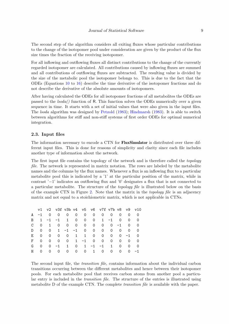
The first input file contains the topology of the network and is therefore called the topologyfile. The network is represented in matrix notation. The rows are labeled by the metabolitenames and the columns by the flux names. Whenever a flux is an inflowing flux to a particularmetabolite pool this is indicated by a ’1’ at the particular position of the matrix, while incontrast ’−1’ indicates an outflowing flux and ’0’ designates a flux that is not connected toa particular metabolite. The structure of the topology file is illustrated below on the basisof the example CTN in Figure 2. Note that the matrix in the topology file is an adjacencymatrix and not equal to a stoichiometric matrix, which is not applicable in CTNs.

v1 v2 v3f v3b v4 v5 v6 v7f v7b v8 v9 v10A -1 0 0 0 0 0 0 0 0 0 0 0B 1 -1 -1 1 0 0 0 1 -1 0 0 0C 0 1 0 0 0 0 0 0 0 -1 0 0D 0 0 1 -1 -1 0 0 0 0 0 0 0E 0 0 0 0 1 1 0 0 0 0 -1 0F 0 0 0 0 1 -1 0 0 0 0 0 0G 0 0 -1 1 0 1 -1 -1 1 0 0 0H 0 0 0 0 0 0 1 0 0 0 0 -1

The second input file, the transition file, contains information about the individual carbontransitions occurring between the different metabolites and hence between their isotopomerpools. For each metabolite pool that receives carbon atoms from another pool a particu-lar entry is included in the transition file. The structure of the entries is illustrated usingmetabolite D of the example CTN. The complete transition file is available with the paper.


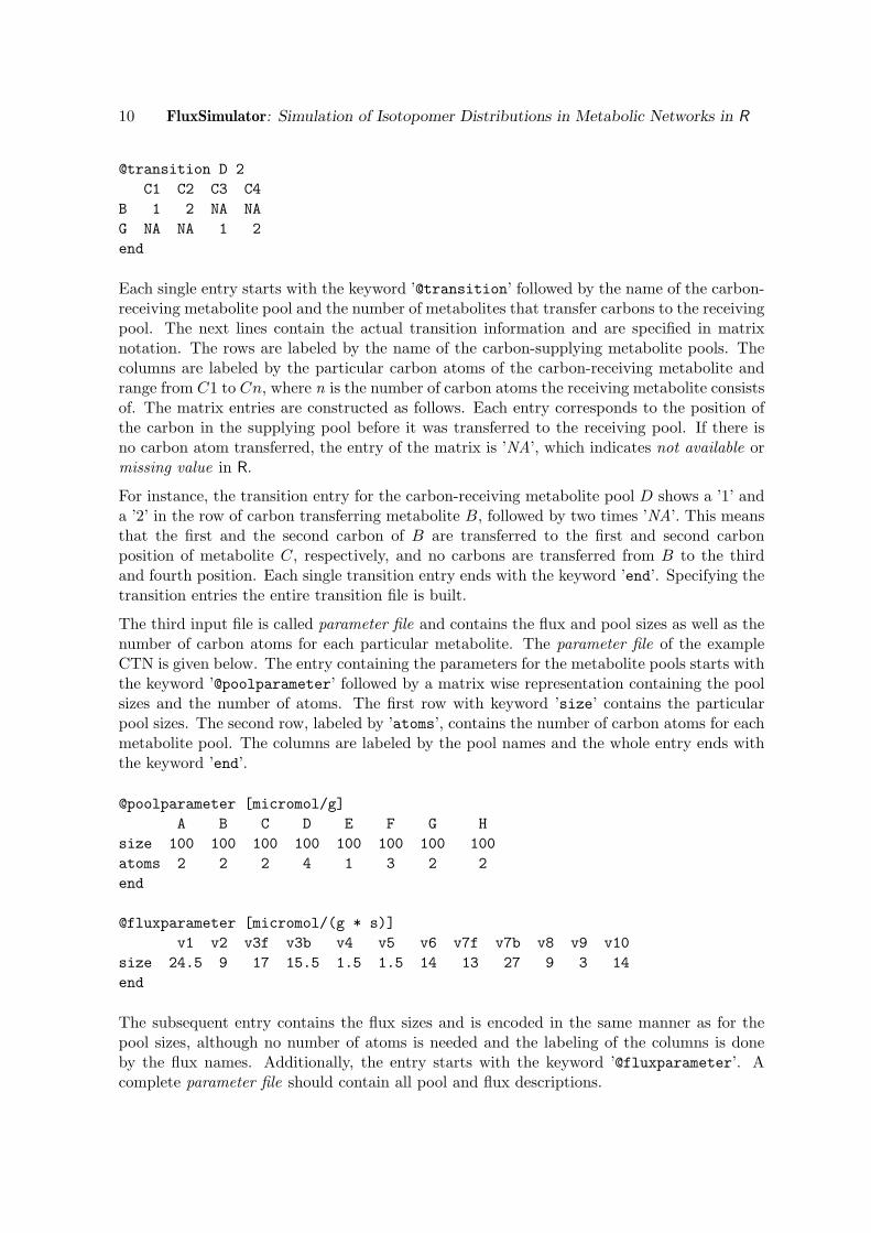
@transition D 2C1 C2 C3 C4

B 1 2 NA NAG NA NA 1 2end

Each single entry starts with the keyword ’@transition’ followed by the name of the carbon-receiving metabolite pool and the number of metabolites that transfer carbons to the receivingpool. The next lines contain the actual transition information and are specified in matrixnotation. The rows are labeled by the name of the carbon-supplying metabolite pools. Thecolumns are labeled by the particular carbon atoms of the carbon-receiving metabolite andrange from C1 to Cn, where n is the number of carbon atoms the receiving metabolite consistsof. The matrix entries are constructed as follows. Each entry corresponds to the position ofthe carbon in the supplying pool before it was transferred to the receiving pool. If there isno carbon atom transferred, the entry of the matrix is ’NA’, which indicates not available ormissing value in R.

For instance, the transition entry for the carbon-receiving metabolite pool D shows a ’1’ anda ’2’ in the row of carbon transferring metabolite B, followed by two times ’NA’. This meansthat the first and the second carbon of B are transferred to the first and second carbonposition of metabolite C, respectively, and no carbons are transferred from B to the thirdand fourth position. Each single transition entry ends with the keyword ’end’. Specifying thetransition entries the entire transition file is built.

The third input file is called parameter file and contains the flux and pool sizes as well as thenumber of carbon atoms for each particular metabolite. The parameter file of the exampleCTN is given below. The entry containing the parameters for the metabolite pools starts withthe keyword ’@poolparameter’ followed by a matrix wise representation containing the poolsizes and the number of atoms. The first row with keyword ’size’ contains the particularpool sizes. The second row, labeled by ’atoms’, contains the number of carbon atoms for eachmetabolite pool. The columns are labeled by the pool names and the whole entry ends withthe keyword ’end’.

@poolparameter [micromol/g]A B C D E F G H

size 100 100 100 100 100 100 100 100atoms 2 2 2 4 1 3 2 2end

@fluxparameter [micromol/(g * s)]v1 v2 v3f v3b v4 v5 v6 v7f v7b v8 v9 v10

size 24.5 9 17 15.5 1.5 1.5 14 13 27 9 3 14end

The subsequent entry contains the flux sizes and is encoded in the same manner as for thepool sizes, although no number of atoms is needed and the labeling of the columns is doneby the flux names. Additionally, the entry starts with the keyword ’@fluxparameter’. Acomplete parameter file should contain all pool and flux descriptions.


2.4. Implementation and application

According to the object-oriented programming style the entire package was designed basedon S4 classes, which are the backbone of object-oriented programming in R (Chambers 2003).They provide all usual object-oriented features such as instantiation, polymorphism and inher-itance. Object oriented programming is very intuitive and structured. Additionally, it offersadvantages when dealing with biological systems, whose modular, hierarchical structure isoften naturally representable in terms of objects.

The FluxSimulator implementation was validated using the CTN given in Figure 2. ThisCTN was specified in the three previously described input files. For comparison the ODErepresentation was also encoded in a file applicable in Berkeley Madonna 8.3.8. It mainlyconsists of the 42 ODEs represented by Equations 10 to 16.

In order to specify the input files correctly, one additional constraint has to be considered.The CTN is assumed to be in metabolic steady state, which means that the pool size ofeach metabolite is not allowed to change over time, although the fractions of its isotopomersare changing. Hence, the flux sizes have to be solutions of the linear equation system inEquation 17 to 23, which results from Equations 1 to 7 with the time derivative set to zero:

v1 + v3b + v7f = v2 + v3f + v7b (17)v2 = v8 (18)

v3f = v4 + v3b (19)v4 + v5 = v9 (20)

v4 = v5 (21)v5 + v3b + v7b = v3f + v6 + v7f (22)

v6 = v10 (23)

This under-determined system of equations guarantees the metabolic steady state. Theamount of all inflowing metabolites is equal to the amount of outflowing metabolites foreach particular metabolite pool. The system consists of seven equations and twelve unknownparameters, the flux sizes. Thus, five flux sizes may be chosen freely and are arbitrarily setto v1 = 24.5

[µmolg·s

], v3f = 17

[µmolg·s

], v7f = 13

[µmolg·s

], v8 = 9

[µmolg·s

]and v9 = 3

[µmolg·s

]in

the example. The remaining seven flux sizes were then computed by solving the system ofequations and resulted in v2 = 9

[µmolg·s

], v3b = 15.5

[µmolg·s

], v4 = 1.5

[µmolg·s

], v5 = 1.5

[µmolg·s

],

v6 = 14[

µmolg·s

], v7b = 27

[µmolg·s

]and v10 = 14

[µmolg·s

].

After the specification of the input files the dynamic behavior of the CTN was simulated inboth packages for a time period of 1000 seconds. The usage of FluxSimulator is describedbelow while the usage of Berkeley Madonna can be found elsewhere (Macey et al. 2000).

The initial step getting started with FluxSimulator is to install and load the FluxSimulatorpackage. Additional packages necessary to install are wle, circular, boot and odesolve which arefreely available on the Comprehensive R Archive Network (CRAN). Once the FluxSimulatorpackage is loaded the function call fluxsim() starts an interactive dialog that guides the userthrough all necessary specifications. This dialog is subsequently explained on the base of theinput necessary to perform the simulation of the example CTN.


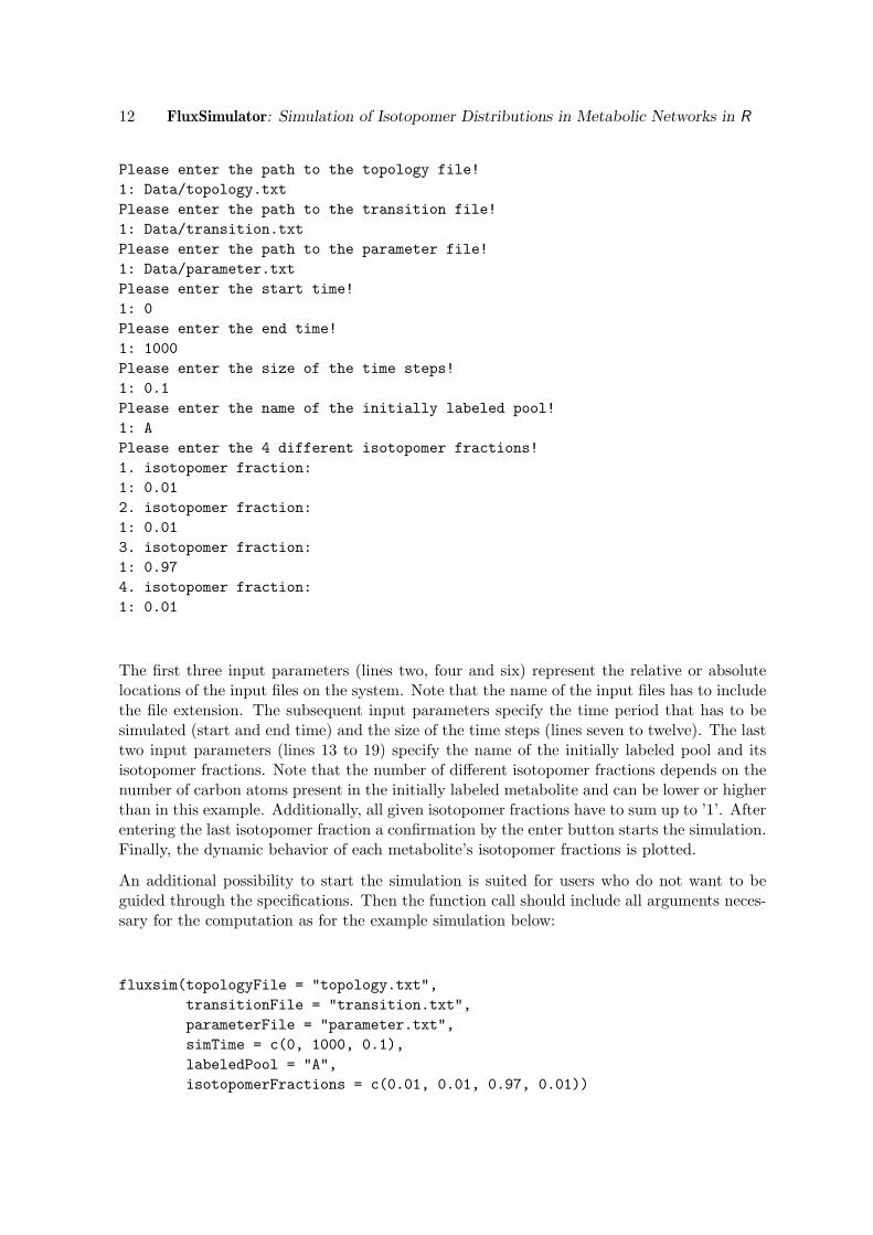
Please enter the path to the topology file!1: Data/topology.txtPlease enter the path to the transition file!1: Data/transition.txtPlease enter the path to the parameter file!1: Data/parameter.txtPlease enter the start time!1: 0Please enter the end time!1: 1000Please enter the size of the time steps!1: 0.1Please enter the name of the initially labeled pool!1: APlease enter the 4 different isotopomer fractions!1. isotopomer fraction:1: 0.012. isotopomer fraction:1: 0.013. isotopomer fraction:1: 0.974. isotopomer fraction:1: 0.01

The first three input parameters (lines two, four and six) represent the relative or absolutelocations of the input files on the system. Note that the name of the input files has to includethe file extension. The subsequent input parameters specify the time period that has to besimulated (start and end time) and the size of the time steps (lines seven to twelve). The lasttwo input parameters (lines 13 to 19) specify the name of the initially labeled pool and itsisotopomer fractions. Note that the number of different isotopomer fractions depends on thenumber of carbon atoms present in the initially labeled metabolite and can be lower or higherthan in this example. Additionally, all given isotopomer fractions have to sum up to ’1’. Afterentering the last isotopomer fraction a confirmation by the enter button starts the simulation.Finally, the dynamic behavior of each metabolite’s isotopomer fractions is plotted.

An additional possibility to start the simulation is suited for users who do not want to beguided through the specifications. Then the function call should include all arguments neces-sary for the computation as for the example simulation below:

fluxsim(topologyFile = "topology.txt",transitionFile = "transition.txt",parameterFile = "parameter.txt",simTime = c(0, 1000, 0.1),labeledPool = "A",isotopomerFractions = c(0.01, 0.01, 0.97, 0.01))


3. Results and discussion

In the following the simulation results of FluxSimulator and Berkeley Madonna achievedduring the simulation of the dynamics of the CTN are compared. Additionally, the handlingand performance of the packages is discussed.

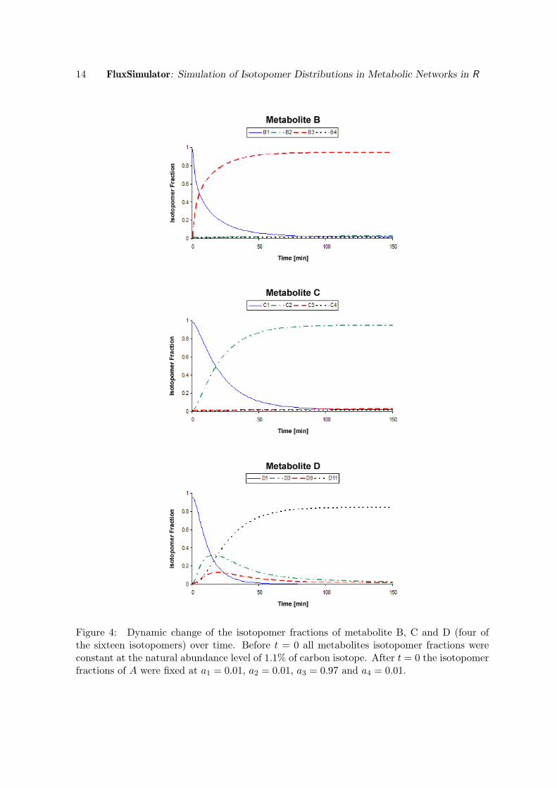
As mentioned previously the numerical integration method chosen for FluxSimulator is thelsoda algorithm of Petzold et al. (Petzold 1983). The algorithm chosen in Berkeley Madonnawas developed by Runge and Kutta (Albrecht 1977). All results achieved during the numer-ical integration with Berkeley Madonna were given to the seventh decimal place behind thedecimal point. Those of FluxSimulator up to the tenth decimal place. It turned out thatboth simulations computed exactly the same results in each iteration step when the valuesof FluxSimulator were rounded to the seventh decimal position. Hence, both simulationscomputed equal dynamic behavior for all isotopomer fractions. This confirmed the adequateperformance of FluxSimulator, for which three example plots are given in Figure 4.

Berkeley Madonna receives one input file in plain text format. Within this input file eachODE describing the behavior of a single isotopomer has to be encoded by hand, leading to atotal of 42 ODEs for the current example. This leads to the following issues:

1. All network properties have to be considered manually, e.g. multimolecular reactionsor the fact that one isotopomer could be fed by more than one isotopomer of anothermetabolite.

2. Small changes in the network can cause various changes in several ODEs that have tobe recoded carefully by hand.

3. Unexperienced users prefer the specification of a more intuitive network representation,above hard-coded equations.

It is clear that manual specification of the ODEs is a potential source of error and leads tolimited flexibility and low biologist-friendliness. This is addressed by FluxSimulator and itsautomatic derivation of the ODEs from the three intuitive input files. These files can beedited easily. Hence, changes in the network can be made very fast and consistently, leadingto a high flexibility of the package. Moreover, the generation of the input files is feasible fora biologist without mathematical and computer science training.

4. Conclusions and outlook

In this work we presented a new R package called FluxSimulator to simulate isotopomer dis-tributions in metabolic networks over time. The package was developed using object-orientedS4 classes. It was specifically designed to derive the mathematical representation underlyingthe dynamics of the network automatically using intuitive input files. FluxSimulator andBerkeley Madonna computed an identical behavior for the example CTN. However, in con-trast to Berkeley Madonna or other available simulation programs, FluxSimulator is suitablefor users with a weak mathematical background. This is due to the fact that the enormouspotential for errors during direct encoding of all ODEs representing a CTN is circumvented.Additionally, the user can more easily and consistently experiment with the model system,


Figure 4: Dynamic change of the isotopomer fractions of metabolite B, C and D (four ofthe sixteen isotopomers) over time. Before t = 0 all metabolites isotopomer fractions wereconstant at the natural abundance level of 1.1% of carbon isotope. After t = 0 the isotopomerfractions of A were fixed at a1 = 0.01, a2 = 0.01, a3 = 0.97 and a4 = 0.01.


e. g. changing the network topology. A web interface for users that want to simulate theirCTNs without installing R is planned and will enhance the user-friendliness.

Hence, FluxSimulator is an appropriate alternative to simulate isotopomer distributions overtime in metabolic networks. Future work will improve and extend FluxSimulator further withspecial focus on the following properties:

1. Incorporation of algorithms to eliminate ODEs not necessary for the computation ofthe desired simulation, hence increasing computational speed.

2. Analysis of experimental NMRS data to estimate the fluxes.

3. Application of the statistical facilities of R to simulate hypothetical NMRS data, e.g.by adding measurement noise.

4. Application of the optimization routines of R to estimate unknown flux parameters fromthe experimental NMRS data.

5. Incorporation of algorithms to improve the speed of solving the ODEs.

6. Increase of flexibility with respect to the input of labeled isotopomers, e.g. usage ofseveral metabolite pools as entry point for labeled substrate, or flexible functions oftime.

7. Extension to other isotopes like 2H, 15N, 17O, 18O and 33S, or a combination of them.

8. Development of a concise and easy to handle graphical user interface to enhance theflexibility and the comfort.

9. Analysis of MS data in combination with NMRS data to estimate the flux parameters.

All these improvements can make FluxSimulator a powerful, flexible and easy to handle toolto analyze and simulate isotope labeling NMRS and MS experiments.

Acknowledgments

This work is part of the BioRange program (project number SP 2.2.1) of the NetherlandsBioinformatics Centre (NBIC), which is supported by a BSIK grant through the NetherlandsGenomics Initiative (NGI). The work is also part of the Center for Medical Systems Biologywhich is a Genomics Center of Excellence funded by the Dutch Government via the NGI.K.M. was supported by Computational Science grant #635.000.014 from the NetherlandsOrganization for Scientific Research (NWO).

References

Albrecht P (1977). “The Runge-Kutta Theory in a Nutshell.” SIAM Journal on NumericalAnalysis, 14, 1006–1021.


Bohm H, Klebe G, Kubinyi H (2002). Wirkstoffdesign - Der Weg zum Arzneimittel. SpektrumAkademischer Verlag, Heidelberg.

Chambers J (2003). Programming with Data: A Guide to the S Language. Springer, Berlin.

Chance E, Seeholzer S, Kobayashi K, Williamson J (1983). “Mathematical Analysis of IsotopeLabeling in the Citric Acid Cycle with Applications to 13C NMR Studies in Perfused RatHearts.” Journal of Biological Chemistry, 258, 13785–13794.

Dunn I, Heinzle E, Ingham J, Jiri E (2003). Biological Reaction Engineering. Dynamic Mod-elling Fundamentals with Simulation Examples. Wiley-VCH Verlag GmbH & Co. KGaA,Weinheim.

Hindmarsh A (1983). “ODEPACK, A Systematized Collection of ODE Solvers.” ScientificComputing, pp. 55–64.

Leach A, Gillet V (2003). An Introduction to Chemoinformatics. Springer, Berlin.

Macey R, Oster G, Zahnley T (2000). Berkeley Madonna User’s Guide. University of Cali-fornia.

Michaelis L, Menten ML (1913). “Die Kinetik der Invertinwirkung.” Biochemische Zeitschrift,49, 333–369.

Nassi I, Shneiderman B (1973). “Flowchart Techniques for Structured Programming.” SIG-PLAN Notices, 8, 12–26.

Petzold L (1983). “Automatic Selection of Methods for Solving Stiff and Nonstiff Systems ofOrdinary Differential Equations.” SIAM Journal on Scientific Computing, 4, 136–148.

Raymond G, Butterworth E, Bassingthwaighte J (2003). “JSIM: Free Software Package forTeaching Phyiological Modeling and Research.” Experimental Biology, 280.5, 102.

R Development Core Team (2006). R: A Language and Environment for Statistical Computing.R Foundation for Statistical Computing, Vienna, Austria. ISBN 3-900051-07-0, URL http://www.R-project.org/.

Sauer F, Erfle J, Binns M (1970). “Turnover Rates and Intracellular Pool Size Distribution ofCitrate Cycle Intermediates in Normal, Diabetic and Fat-Fet Rats Estimated by ComputerAnalysis from Specific Activity Decay Data of 14C-Labeled Citrate Cycle Acids.” EuropeanJournal of Biochemistry, 17, 350–363.

van Beek JM, Csont T, de Kanter F, Bussemaker J (1998). “Simple Model Analysis of 13CNMR Spectra to Measure Oxygen Consumption Using Frozen Tissue Samples.” Advancesin Experimental Medicine and Biology, 454, 475–485.

van Beek JM, van Mil H, King R, de Kanter F, Alders D, Bussemaker J (1999). “A 13C NMRDouble-Labeling Method to Quantitate Local Myocardial O2 Consumption Using FrozenTissue Samples.” American Journal of Physiology, 277, H1630–H1640.

Wiechert W (2001). “13C Metabolic Flux Analysis.” Metabolic Engineering, 3, 195–206.

http://www.R-project.org/

http://www.R-project.org/


Wiechert W, de Graaf A (1997). “Bidirectional Reaction Steps in Metabolic Networks: I.Modeling and Simulation of Carbon Isotope Labeling Experiments.” Biotechnology andBioengineering, 55, 101–117.

Wiechert W, de Graaf A, Marx A (1995). “In Vivo Stationary Flux Determination Using 13CNMR Isotope Labelling Experiments.” Advances in Biochemical Engineering/Biotechnol-ogy, 54, 109–154.

Wiechert W, Mollney M, Isermann N, Wurzel M, de Graaf A (1999). “Bidirectional ReactionSteps in Metabolic Networks: III. Explicit Solution and Analysis of Isotopomer LabelingSystems.” Biotechnology and Bioengineering, 66, 71–85.

Wiechert W, Mollney M, Petersen S, de Graaf A (2001). “A Universal Framework for 13CMetabolic Flux Analysis.” Metabolic Engineering, 3, 265–283.

Wiechert W, Siefke C, de Graaf A, Marx A (1997). “Bidirectional Reaction Steps in MetabolicNetworks: II. Flux Estimation and Statistical Analysis.” Biotechnology and Bioengineering,55, 118–135.

Affiliation:

Thomas W. BinslFaculteit der Exacte WetenschappenVrije Universiteit AmsterdamDe Boelelaan 1083a1081HV Amsterdam, The NetherlandsTelephone: +31/02/5987734 E-mail: [email protected]: http://www.few.vu.nl/~tbinsl/

Journal of Statistical Software http://www.jstatsoft.org/published by the American Statistical Association http://www.amstat.org/

Volume 18, Issue 7 Submitted: 2006-09-28January 2007 Accepted: 2007-01-10

mailto:[email protected]

http://www.few.vu.nl/~tbinsl/

http://www.jstatsoft.org/

http://www.amstat.org/

Documents

FluxSimulator: An R Package to Simulate Isotopomer