Embed Size (px)
Citation preview
Colliders : pp – LEP – pp FNSN 2 - Chapter 8
Paolo Bagnaia
last mod. 6-May-17
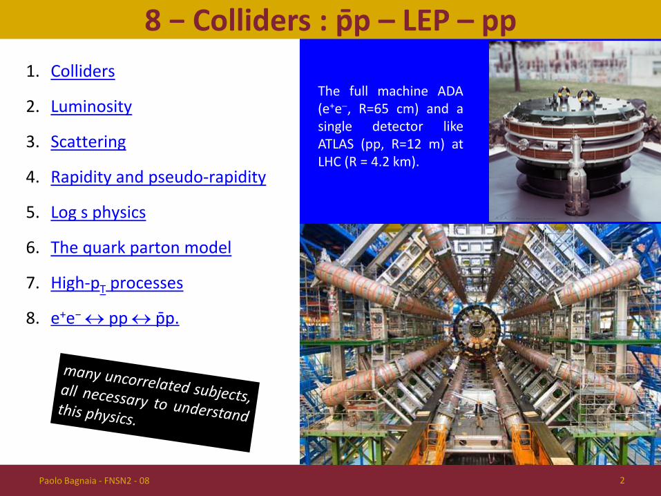
The full machine ADA (e+e−, R=65 cm) and a single detector like ATLAS (pp, R=12 m) at LHC (R = 4.2 km).
8 − Colliders : pp – LEP – pp 1. Colliders
2. Luminosity
3. Scattering
4. Rapidity and pseudo-rapidity
5. Log s physics
6. The quark parton model
7. High-pT processes
8. e+e− ↔ pp ↔ pp.
Paolo Bagnaia - FNSN2 - 08 2
Colliders : introduction • Hadronic collisions (Spp S + LHC at
CERN, TeVatron at Fermilab) share common dynamical and kinematical features, different from e+e− (Spear, LEP, …).
• Hadrons are composite, as explained by the QCD-quark-parton model : coherent pp (p p) scattering at low pT; qq/qq /qg/q g/gg scattering at high pT,
dominated by t-channel gg.
• Instead in e+e− Colliders only point-like interactions, dominated by s-channel.
• The historical order Spp S – LEP – LHC is unnatural (hadrons, leptons, hadrons), but we will follow it, at the price of some repetitions and logical leaps.
• In the Spp S and LHC chapters, the order will be the traditional one, increasing pT and decreasing cross-section :
1. [total cross-section], 2. low-pT interactions, 3. high-pT hadronic processes, 4. high-pT electro-weak; 5. [searches for new physics, if any].
• For LEP, the order will be the history, i.e. the increasing beam energy : 1. Z-pole electroweak physics, 2. W+W− pair creation, 3. [a digression on the method of
searches and the analysis of negative results, the "limits"],
4. Higgs searches; 5. [searches for new physics, if any].
• In this first chapter, there are some definitions and discussions, useful for all the following parts, especially for hadron colliders.
1/7
Paolo Bagnaia - FNSN2 - 08 3
Colliders : vs fixed target
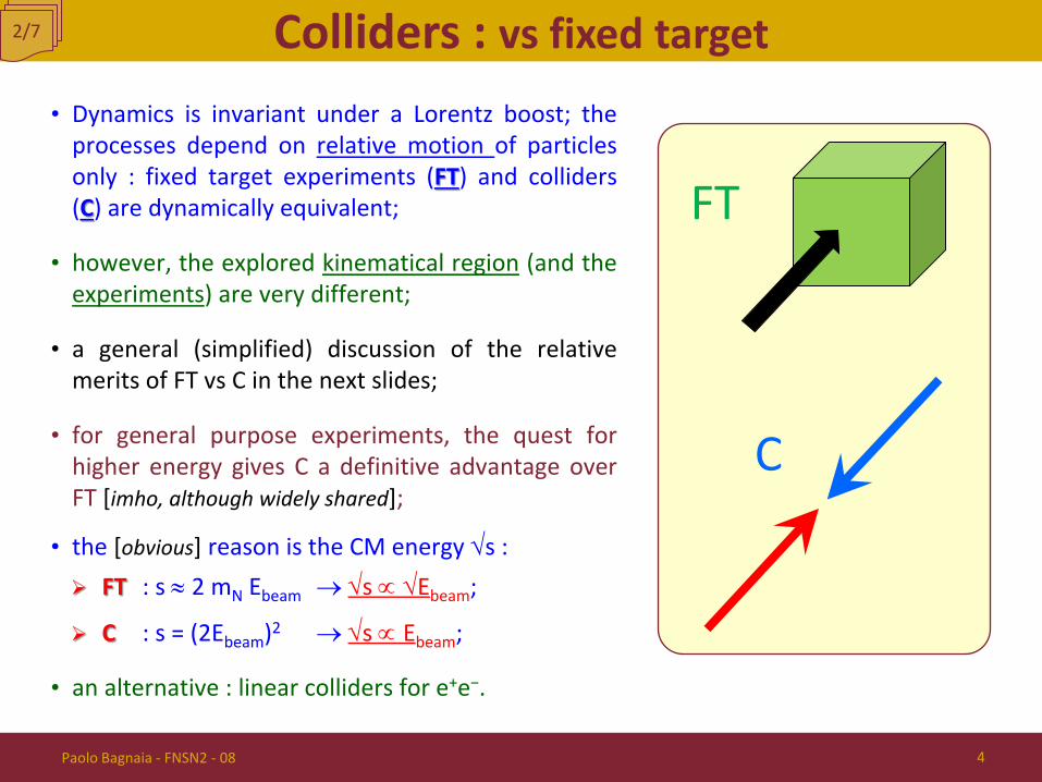
• Dynamics is invariant under a Lorentz boost; the processes depend on relative motion of particles only : fixed target experiments (FT) and colliders (C) are dynamically equivalent;
• however, the explored kinematical region (and the experiments) are very different;
• a general (simplified) discussion of the relative merits of FT vs C in the next slides;
• for general purpose experiments, the quest for higher energy gives C a definitive advantage over FT [imho, although widely shared];
• the [obvious] reason is the CM energy √s : FT : s ≈ 2 mN Ebeam → √s ∝ √Ebeam;
C : s = (2Ebeam)2 → √s ∝ Ebeam;
• an alternative : linear colliders for e+e−.
2/7
FT
C
Paolo Bagnaia - FNSN2 - 08 4
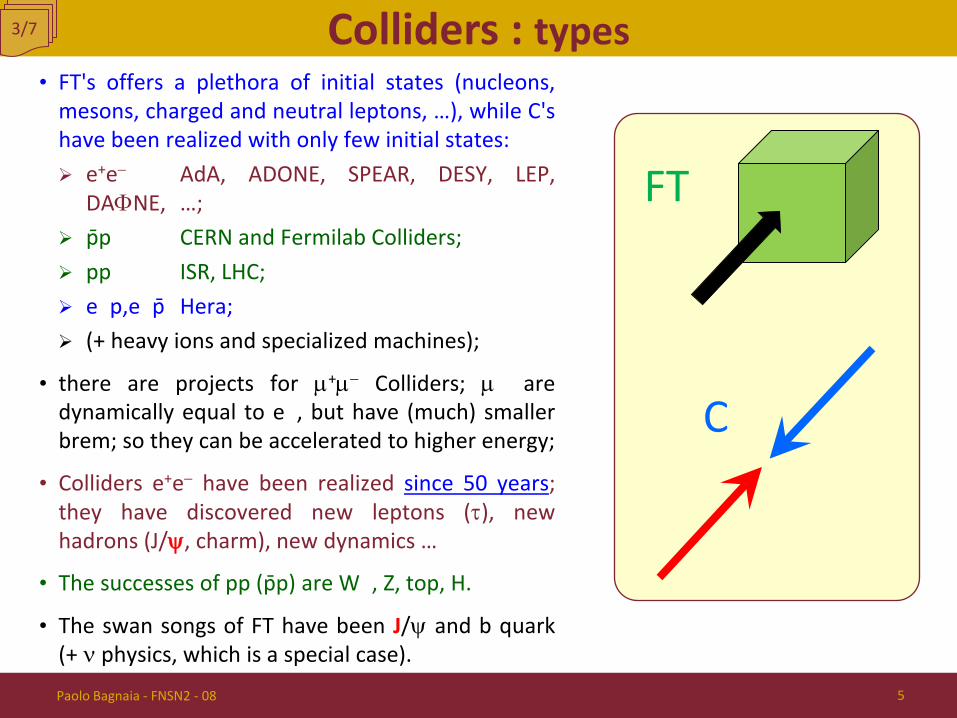
Colliders : types • FT's offers a plethora of initial states (nucleons,
mesons, charged and neutral leptons, …), while C's have been realized with only few initial states: e+e− AdA, ADONE, SPEAR, DESY, LEP,
DAΦNE, …; p p CERN and Fermilab Colliders; pp ISR, LHC; e±p,e±p Hera; (+ heavy ions and specialized machines);
• there are projects for µ+µ− Colliders; µ± are dynamically equal to e±, but have (much) smaller brem; so they can be accelerated to higher energy;
• Colliders e+e− have been realized since 50 years; they have discovered new leptons (τ), new hadrons (J/ψ, charm), new dynamics …
• The successes of pp (p p) are W±, Z, top, H.
• The swan songs of FT have been J/ψ and b quark (+ ν physics, which is a special case).
3/7
FT
C
Paolo Bagnaia - FNSN2 - 08 5
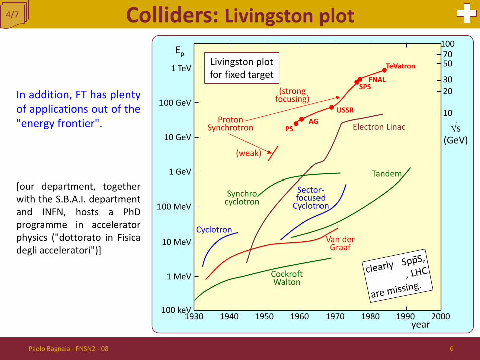
Colliders: Livingston plot
In addition, FT has plenty of applications out of the "energy frontier".
[our department, together with the S.B.A.I. department and INFN, hosts a PhD programme in accelerator physics ("dottorato in Fisica degli acceleratori")]
4/7
1930 1940 1950 1960 1970 1980 1990 2000
100 GeV
1 TeV
10 GeV
1 GeV
100 MeV
10 MeV
1 MeV
100 keV
10
20 30
50 70
100
√s (GeV)
Ep
Cockroft Walton
Van der Graaf
Tandem
Sector- focused
Cyclotron
(strong focusing)
Synchro cyclotron
Cyclotron
Electron Linac
(weak)
Proton Synchrotron PS
AG USSR
SPS FNAL
TeVatron
year
Livingston plot for fixed target
Paolo Bagnaia - FNSN2 - 08 6
Colliders: synchrotron
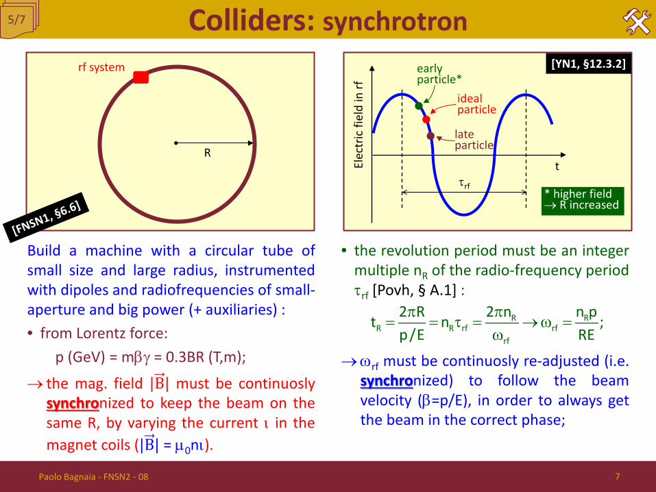
Paolo Bagnaia - FNSN2 - 08 7
Build a machine with a circular tube of small size and large radius, instrumented with dipoles and radiofrequencies of small-aperture and big power (+ auxiliaries) : • from Lorentz force: p (GeV) = mβγ = 0.3BR (T,m);
→ the mag. field |B| must be continuosly synchronized to keep the beam on the same R, by varying the current ι in the magnet coils (|B| = µ0nι).
• the revolution period must be an integer multiple nR of the radio-frequency period τrf [Povh, § A.1] :
→ ωrf must be continuosly re-adjusted (i.e. synchronized) to follow the beam velocity (β=p/E), in order to always get the beam in the correct phase;
π π= = τ = → ω =
ωR R
R R rf rfrf
2 R 2 n n pt n ;p/E RE
R
rf system
t Elec
tric
fiel
d in
rf
τrf
ideal particle
early particle*
late particle
* higher field → R increased
[YN1, §12.3.2]
5/7
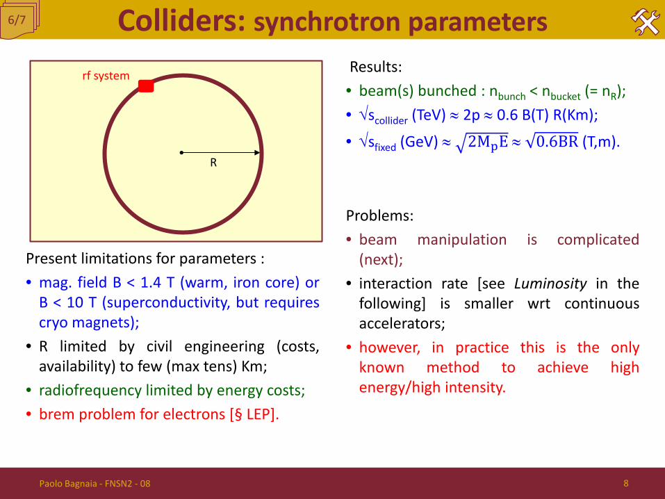
Colliders: synchrotron parameters
Paolo Bagnaia - FNSN2 - 08 8
Present limitations for parameters : • mag. field B < 1.4 T (warm, iron core) or
B < 10 T (superconductivity, but requires cryo magnets);
• R limited by civil engineering (costs, availability) to few (max tens) Km;
• radiofrequency limited by energy costs; • brem problem for electrons [§ LEP].
Results: • beam(s) bunched : nbunch < nbucket (= nR); • √scollider (TeV) ≈ 2p ≈ 0.6 B(T) R(Km);
• √sfixed (GeV) ≈ 2MpE ≈ 0.6BR (T,m).
Problems: • beam manipulation is complicated
(next); • interaction rate [see Luminosity in the
following] is smaller wrt continuous accelerators;
• however, in practice this is the only known method to achieve high energy/high intensity.
R
rf system
6/7
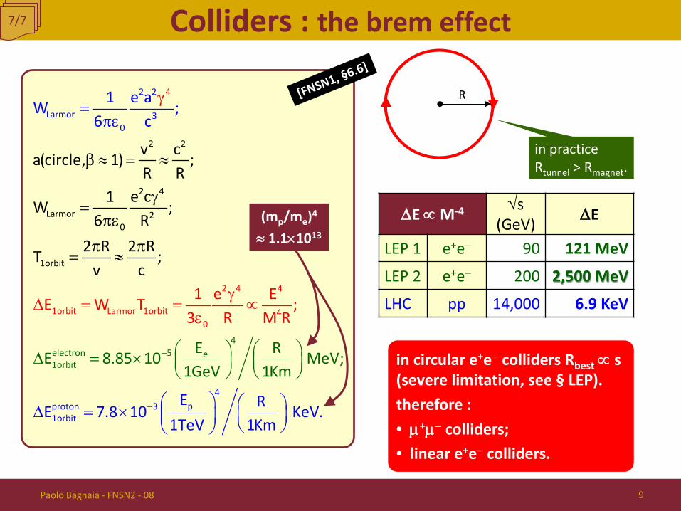
Colliders : the brem effect 7/7
R
Paolo Bagnaia - FNSN2 - 08 9
∆E ∝ M-4 √s (GeV) ∆E
LEP 1 e+e− 90 121 MeV
LEP 2 e+e− 200 2,500 MeV
LHC pp 14,000 6.9 KeV
in circular e+e− colliders Rbest ∝ s (severe limitation, see § LEP). therefore : • µ+µ− colliders; • linear e+e− colliders.
−
−
γ
γ
β
=πε
∆
∆ = = ∝ε
≈ =
∆ = ×
≈
γ=
πεπ π
= ≈
= ×
4
2 4 4
1orbit Larmor 1
4electron 5 e1orbi
orbit
2 2
Larmor 30
proton 31orbit
2 2
2 4
Lar
t
mor
4
20
1orbi
0
t
v ca(circle, 1) ;R R
1 e cW ;
E RE 8.85 10
1 e EE W T ;3 R M R
6 R2 R
1 e aW ;6 c
MeV;1GeV
E 7.8
1K
2
m
R ;c
10
Tv
4pE R KeV.
1TeV 1Km
(mp/me)4 ≈ 1.1×10¹³
in practice Rtunnel > Rmagnet.

The fundamental figure to quantify collider performances of a collider is the Luminosity. Define it with a toy model:
•N1 particles/bunch turning "clockwise"; •N2 … "anti-clockwise";
• cylindrical bunches S×ℓ, ρ = const. [this is the toy assumption];
• for each of N1, while traveling inside the cylinder N2 for a small step x, the probability of interaction is:
℘1(x) = 1 - e-ρσTx ≅ ρ σT x = N2σTx/(S ℓ);
• the average number of interactions / crossing is :
<nI> = N1 ℘1(ℓ) = N1 N2 σT / S; [<nI> independent from ℓ] • the crossings rate is nc = k × ƒ [k = bunch number, ƒ = revolution frequency] therefore, the interaction rate is : R ≡ L σT = <nI> × nc = N1 N2 k ƒ σT / S, where L, called the "luminosity",
contains the parameters of the machine, while σT reflects the particle dynamics:
Luminosity: toy model 1/11
= 1 toy 2NS
N kƒ . L
Paolo Bagnaia - FNSN2 - 08 10
1 2 3
A B C
ℓ
← N2 S N1 • →

Luminosity: comments 2/11
=πσ σ1
x
2
y
kƒ .4
NNL
Paolo Bagnaia - FNSN2 - 08 11
The toy model is too naïve, however some of the conclusions are correct. The luminosity, defined as L ≡ R/σT, the ratio between the interaction rate and the total cross section(*), is : • NOT dependent (for head-on collisions) on the bunch length ℓ;
• proportional to the inverse of the bunch section (use an effective bunch section S = 4πσxσy);
• proportional to the number of particles / bunch of both beams (N1N2);
• proportional to the number of bunch crossings / second (kƒ);
• [not in formula] dependent on centroids displacement and beam lifetime.
___________________________ (*) for a process x : Rx/RT = σx/σT → Rx=L σx.
NB the total number of interactions seems to grow ∝ k2; however, in a given interaction point, it grows ∝ k. Is it clear ? from this consideration, many clever machine developments, e.g. the pretzel scheme.
1 2 3
A B C
ℓ
N1 • → S
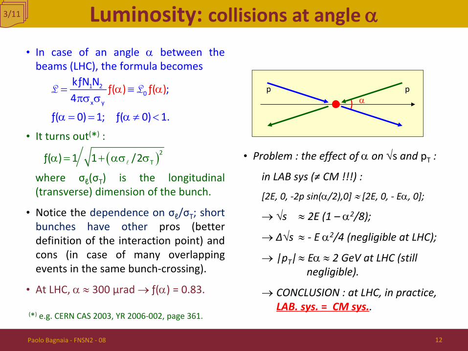
Luminosity: collisions at angle α
• In case of an angle α between the beams (LHC), the formula becomes
• It turns out(*) :
where σℓ(σT) is the longitudinal (transverse) dimension of the bunch.
• Notice the dependence on σℓ/σT; short bunches have other pros (better definition of the interaction point) and cons (in case of many overlapping events in the same bunch-crossing).
• At LHC, α ≈ 300 μrad → ƒ(α) = 0.83.
(*) e.g. CERN CAS 2003, YR 2006-002, page 361.
• Problem : the effect of α on √s and pT :
in LAB sys (≠ CM !!!) :
[2E, 0, -2p sin(α/2),0] ≈ [2E, 0, - Eα, 0];
→ √s ≈ 2E (1 – α2/8);
→ ∆√s ≈ - E α2/4 (negligible at LHC);
→ |pT| ≈ Eα ≈ 2 GeV at LHC (still negligible).
→ CONCLUSION : at LHC, in practice, LAB. sys. = CM sys..
α p p
3/11
= ≡πσ σ
α =
α α
= α ≠ <
1 20
x y
ƒ( ) ƒ( )kƒN N ;4
ƒ( 0) 1; ƒ( 0) 1.
L L
( )α = + ασ σ
2Tƒ( ) 1 1 /2
Paolo Bagnaia - FNSN2 - 08 12
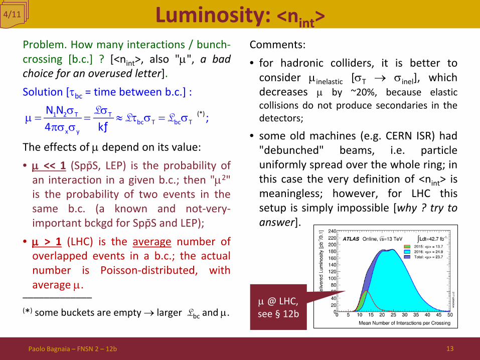
Luminosity: <nint> Problem. How many interactions / bunch-crossing [b.c.] ? [<nint>, also "µ", a bad choice for an overused letter]. Solution [τbc = time between b.c.] : The effects of µ depend on its value: • µ << 1 (SppS, LEP) is the probability of
an interaction in a given b.c.; then "µ2" is the probability of two events in the same b.c. (a known and not-very-important bckgd for SppS and LEP);
• µ > 1 (LHC) is the average number of overlapped events in a b.c.; the actual number is Poisson-distributed, with average µ.
_____________ (*) some buckets are empty → larger Lbc and µ.
Comments: • for hadronic colliders, it is better to
consider µinelastic [σT → σinel], which decreases µ by ~20%, because elastic collisions do not produce secondaries in the detectors;
• some old machines (e.g. CERN ISR) had "debunched" beams, i.e. particle uniformly spread over the whole ring; in this case the very definition of <nint> is meaningless; however, for LHC this setup is simply impossible [why ? try to answer].
4/11
Paolo Bagnaia – FNSN 2 – 12b 13
σ σµ = = ≈ τ σ = σ
πσ σ1 2 T T
bc T bc Tx
(
y
*)N N ;4 k
LL L
ƒ
µ @ LHC, see § 12b

Luminosity : ε, β, β* The dynamics of a real beam : • real particles oscillate around the ideal
trajectory (betatron oscillations);
• Reference system and definitions : z : line of flight of the ideal particle; x,y : deflections from ideal orbit; x' ≡ px / pz; y' ≡ py / pz; σx ≡ rms beam size in x (also σy, σx', σy'); εx = π · σx · σx’ = "transverse emittance"; βx = σx / σx’ = "amplitude function"; εy = π · σy · σy’ ; βy = σy / σy’ .
• Therefore (for the *, see on this page):
• From Liouville's theorem : V(6-dim) = σx· σy· σz· σpx· σpy· σpz =
= constant; εx,y = const. (modulo stochastic effects,
which increase it with time); βx,y can be modified by accelerator
devices (e.g. quadrupoles) : it MUST be SMALL in the interaction regions ("low-beta", β*), and large far from them ("high-beta", β) [next slide].
z
x,y
5/11
= α = απσ σ ε β ε β
1 2 1 2* *
x y x x y y
kƒN N k N Nƒ( ) ƒ( );4 4
Lƒ
Paolo Bagnaia - FNSN2 - 08 14
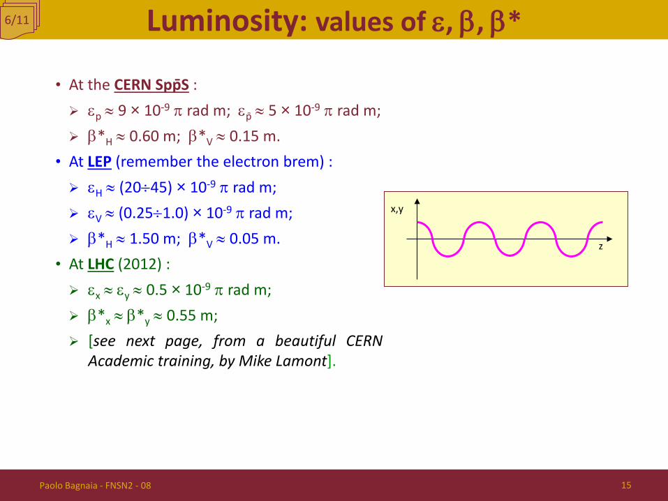
Luminosity: values of ε, β, β*
• At the CERN SppS : εp ≈ 9 × 10⁻⁹ π rad m; εp ≈ 5 × 10⁻⁹ π rad m; β*H ≈ 0.60 m; β*V ≈ 0.15 m.
• At LEP (remember the electron brem) : εH ≈ (20÷45) × 10-9 π rad m; εV ≈ (0.25÷1.0) × 10-9 π rad m; β*H ≈ 1.50 m; β*V ≈ 0.05 m.
• At LHC (2012) : εx ≈ εy ≈ 0.5 × 10⁻⁹ π rad m; β*x ≈ β*y ≈ 0.55 m; [see next page, from a beautiful CERN
Academic training, by Mike Lamont].
z
x,y
6/11
Paolo Bagnaia - FNSN2 - 08 15

Luminosity : β squeeze
Image courtesy John Jowett
β* = 60 cm NB: round beams at IP
βmax ~4.5 km ATLAS @ LHC
7/11
Paolo Bagnaia - FNSN2 - 08 16

Luminosity: better toy model A mechanical analogy [Ed Wilson, 28] : • assume a little ball on a falling guide; • there are two forces :
1. gravity toward z (= "acceleration"); 2. a force orthogonal to z, which depends
on the local shape of the guide (could be elastic, i.e. ∝ |x|);
• Therefore, with parameters ε, β to describe the motion :
• It turns out :
• the area of the ellipses is πε; • β is the ratio between the semi-axes (x/x’).
8/11
= εβ β + φ
≡ ∂ ∂ = ε β β + φ
x sin(z/ );
x' x / z / cos(z/ );
2 2x / x'/ / 1. εβ + ε β =
Paolo Bagnaia - FNSN2 - 08 17
x
x’
z
x 2πβ
ε β/
εβ
εβ
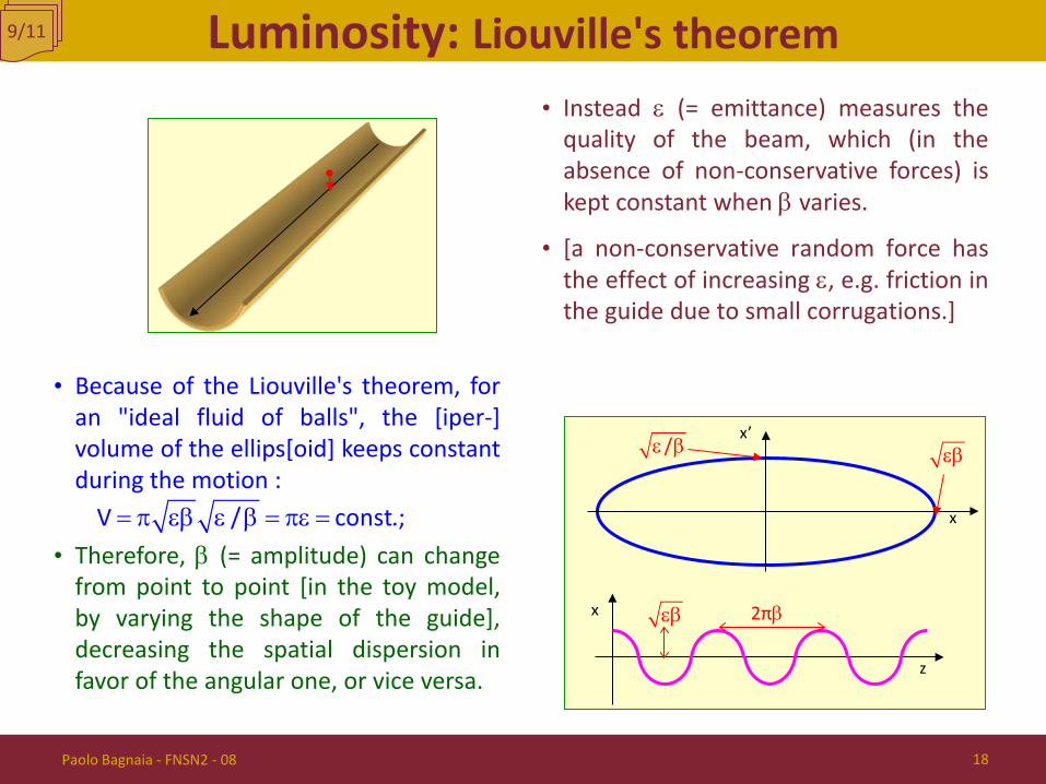
Luminosity: Liouville's theorem
• Because of the Liouville's theorem, for an "ideal fluid of balls", the [iper-] volume of the ellips[oid] keeps constant during the motion :
• Therefore, β (= amplitude) can change from point to point [in the toy model, by varying the shape of the guide], decreasing the spatial dispersion in favor of the angular one, or vice versa.
• Instead ε (= emittance) measures the quality of the beam, which (in the absence of non-conservative forces) is kept constant when β varies.
• [a non-conservative random force has the effect of increasing ε, e.g. friction in the guide due to small corrugations.]
9/11
V / const.;= π εβ ε β = πε =
Paolo Bagnaia - FNSN2 - 08 18
x
x’
z
x 2πβ
ε β/
εβ
εβ

Luminosity: evolution with time
• Many effects deteriorate the luminosity during a long data-taking. [following figures from LHC, but the effects are similar for all colliders].
• Parameterize as dL = -L dt/τi; at LHC : collisions τcoll ≅ 29 h; increase of emittance τIBS ≅ 80 h; residual gas τgas ≅ 100 h; (many other minor effects ...)
• Global effect on luminosity :
L(t)=Lmaxe(-t/τ) ;
1τ = ∑ 1
τj ≈ 1 / (15 h).
• Integrated luminosity after a time T :
• After few hours, new injection and acceleration [see § LHC].
• I.e. effective luminosity ≈ max × 0.5.
• The "decision" to dump the beam and restart the cycle (inject − accelerate − squeeze − data-taking) is crucial : At the Spp S was dramatic (high level
officials), due the scarcity of p . Even at LHC (plenty of protons
everywhere) is a major concern.
1.00
20 10 5 0 15 .00
.50
.75
.25
L(t) / L0
t (h)
10/11
− τ = ≈ τ −
= ⋅σ = ⋅σ
∫∫
T (T / )INT MAX0
T
TOT INT TOT0
(T) (t)dt 1 e ;
N(T) (t) dt (T) .
L L L
L L
Paolo Bagnaia - FNSN2 - 08 19
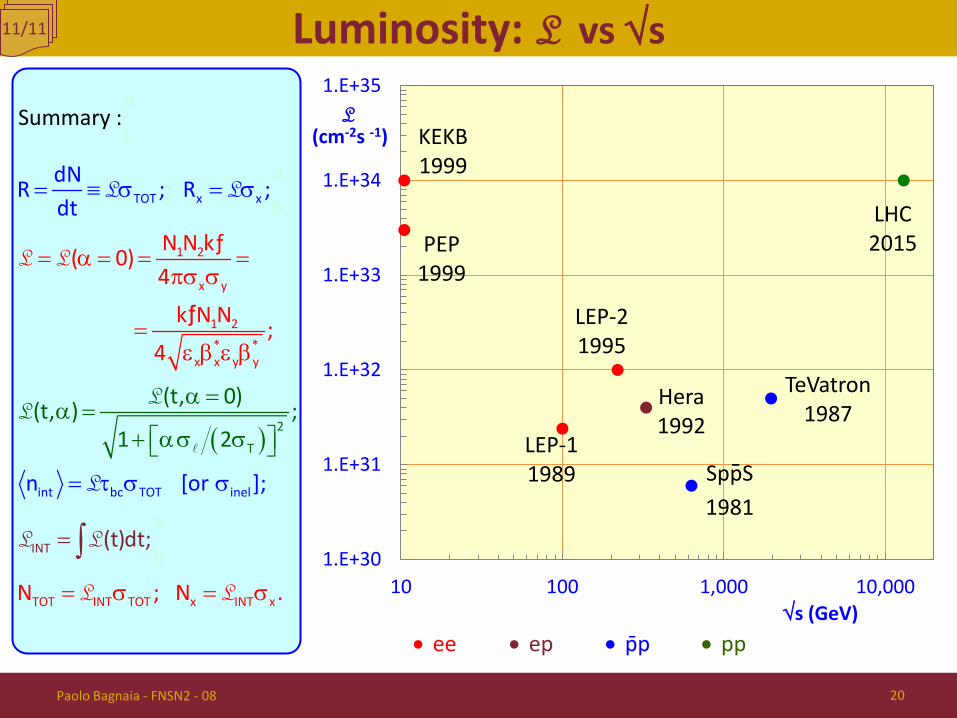
Luminosity: L vs √s 11/11
Paolo Bagnaia - FNSN2 - 08 20
Spp S 1981
TeVatron 1987
Hera 1992
LHC 2015
LEP-2 1995
PEP 1999
KEKB 1999
LEP-1 1989
1.E+30
1.E+31
1.E+32
1.E+33
1.E+34
1.E+35
10 100 1,000 10,000
L (cm-2s -1)
√s (GeV) • ee • ep • p p • pp
( )
= α = =
α =α =
+ ασ σ
=
=
≡ σ =
=πσ σ
=ε β ε β
= σ =
σ
=
σ
τ σ σ
∫
1
TO
2
T
T x x
int bc TO
2
x y
1 2* *
x x y y
TOT INT TOT x INT
T inel
IN
x
T
(t, 0)(t
Summaab
adNR ; R ;dt
n [or ]
(t)dt
N N kƒ( 0)4
k N N ;4
N ; N .
a
;
b
ab
, ) ;
;
1
y
b
:
2
r
L
L L
L L
L L
L
L
LL
ƒ
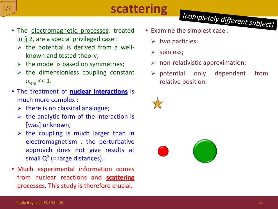
scattering • The electromagnetic processes, treated
in § 2, are a special privileged case : the potential is derived from a well-
known and tested theory; the model is based on symmetries; the dimensionless coupling constant
αem << 1. • The treatment of nuclear interactions is
much more complex : there is no classical analogue; the analytic form of the interaction is
[was] unknown; the coupling is much larger than in
electromagnetism : the perturbative approach does not give results at small Q2 (= large distances).
• Much experimental information comes from nuclear reactions and scattering processes. This study is therefore crucial.
• Examine the simplest case : two particles; spinless; non-relativistic approximation; potential only dependent from
relative position.
Paolo Bagnaia - FNSN2 - 08 21
1/7
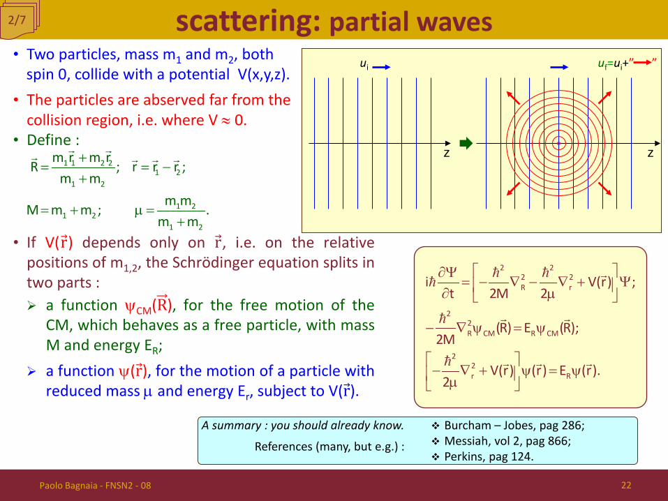
scattering: partial waves • Two particles, mass m1 and m2, both
spin 0, collide with a potential V(x,y,z). • The particles are abserved far from the
collision region, i.e. where V ≈ 0. • Define :
• If V(r) depends only on r, i.e. on the relative positions of m1,2, the Schrödinger equation splits in two parts : a function ψCM(R), for the free motion of the
CM, which behaves as a free particle, with mass M and energy ER;
a function ψ(r), for the motion of a particle with reduced mass µ and energy Er, subject to V(r).
A summary : you should already know.
References (many, but e.g.) :
Burcham – Jobes, pag 286; Messiah, vol 2, pag 866; Perkins, pag 124.
z z
ui uf=ui+” ”
2/7
+= = −
+
= + µ =+
1 1 2 21 2
1 2
1 21 2
1 2
m r m rR ; r r r ;
m mm m
M m m ; .m m
∂Ψ= − ∇ − ∇ + Ψ ∂ µ
− ∇ ψ = ψ
− ∇ + ψ = ψ µ
2 22 2R r
22R CM R CM
22r R
i V(r) ;t 2M 2
(R) E (R);2M
V(r) (r) E (r).2
Paolo Bagnaia - FNSN2 - 08 22
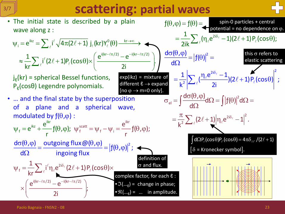
scattering: partial waves • The initial state is described by a plain
wave along z :
jℓ(kr) = spherical Bessel functions, Pℓ(cosθ) Legendre polynomials.
• … and the final state by the superposition of a plane and a spherical wave, modulated by ƒ(θ,ϕ) :
3/7
→∞
− π − − π
ψ = = π + θ →
−≈ + θ ×
∑
∑
krikz 0i
i(kr /2) i(kr /2)
e i 4 (2 1) j (kr)Y ( )
1 e e i (2 1)P (cos ) .kr 2i
δ
− π − − π
ψ = ψ − ψ = θ ϕ
ψ = η + θ ×
−
σ θ ϕ θ ϕ=
ψ = + θ
=
ϕ
×
θ ϕΩ
∑
ikrscattf f i
2if
i(kr /2) i(kr /2)
2
ikrikz
f
d ( , ) outgoing flux@( , ) ƒ( , ) ;d ingoing fl
e ƒ( , );r
1 i e (2 1)P (cos )kr
e e
ee ƒ( ,
;2i
u
; )r
x
Paolo Bagnaia - FNSN2 - 08 23
δ
δ
δ
θ ϕ = θ =
= η −
σ θ ϕσ =
σ θ ϕ= θ =
Ω
η
Ω = θ Ω =Ω
π= + η
−= +
+
−
θ
θ
∫ ∫
∑
∑
∑
2
22
2el
22i2
2
2i
i
ƒ( , ) ƒ( )1 ( e 1)(
d ( , )d ƒ(
2 1)P (cos );2
) dd
d ( , ) ƒ( )d
1 e 1 ( )
(2 1)
(2 1
ik
e
)P (cos ) ;
k
k 2i
1 .
[ ]Ω θ θ = πδ +
δ∫
' 'd P (cos )P (cos ) 4 /(2 1)
= Kronecker symbol .
complex factor, for each ℓ : • ℑ(…ℓ) = change in phase; • ℜ(…ℓ) = … in amplitude.
spin-0 particles + central potential = no dependence on ϕ.
exp(ikz) = mixture of different ℓ → expand [no ϕ → m=0 only].
definition of σ and flux.
this σ refers to elastic scattering
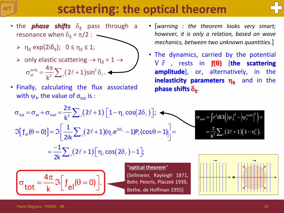
• the phase shifts δℓ pass through a resonance when δℓ = π/2 :
ηℓ exp(2iδℓ); 0 ≤ ηℓ ≤ 1;
only elastic scattering → ηℓ = 1 →
• Finally, calculating the flux associated with ψf, the value of σtot is :
• [warning : the theorem looks very smart; however, it is only a relation, based on wave mechanics, between two unknown quantities.]
• The dynamics, carried by the potential V(r) , rests in ƒ(θ) [the scattering amplitude], or, alternatively, in the inelasticity parameters ηℓ and in the phase shifts δℓ.
scattering: the optical theorem
"optical theorem" [Sellmeier, Rayleigh 1871, Bohr, Peierls, Placzek 1939, Bethe, de Hoffman 1955]
4/7
( ) ( )
[ ] ( )
( ) ( )
δ
πσ = σ + σ = + − η δ
ℑ θ = = ℑ + η − θ = = −
= + η δ −
∑
∑
∑
tot el inel 2
2iel
2 2 1 1 cos 2 ;k1ƒ ( 0) 2 1 ( e 1)P (cos 1)
2ik1 2 1 cos 2 1 ;
2k
π σ = ℑ θ = 4 ƒ ( 0) .tot elk
Paolo Bagnaia - FNSN2 - 08 24
( )πσ = + δ∑
only 2el 2
4 2 1 sin .k
( )( )( )
σ = Ω ψ − ψ =
π= + − η
∫
∑
222 scattinel i f
22
r d
2 1 1 .k
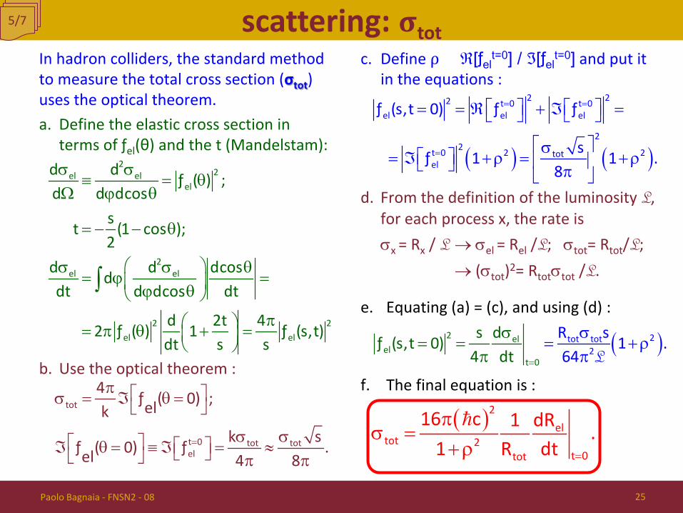
scattering: 𝛔tot In hadron colliders, the standard method to measure the total cross section (σtot) uses the optical theorem. a. Define the elastic cross section in
terms of ƒel(θ) and the t (Mandelstam):
b. Use the optical theorem :
c. Define ρ = ℜ[ƒelt=0] / ℑ[ƒel
t=0] and put it in the equations :
d. From the definition of the luminosity L, for each process x, the rate is
σx = Rx / L → σel = Rel /L; σtot= Rtot/L;
→ (σtot)2= Rtotσtot /L.
e. Equating (a) = (c), and using (d) :
f. The final equation is :
5/7
σ σ≡ = θ
Ω ϕ θ
= − − θ
σ σ θ= ϕ = ϕ θ
π = π θ + =
∫
22el el
el
2el el
2 2el el
d d ƒ ( ) ;d d dcos
st (1 cos );2
d d dcosddt d dcos dt
d 2t 42 ƒ ( ) 1 ƒ (s,t)dt s s
=
π σ = ℑ θ =
σ σ ℑ θ = ≡ ℑ = ≈ π π
tot
t 0 tot totel
4 ƒ ( 0) ;elkk sƒ ( 0) ƒ .el 4 8
( ) ( )
= =
=
= = ℜ + ℑ =
σ = ℑ + ρ = + ρ π
2 22 t 0 t 0el el el
22t 0 2 2tot
el
ƒ (s,t 0) ƒ ƒ
s ƒ 1 1 .8
( )=
σ= =
πσ
= + ρπ
2 elel
t
2tot tot
02
s dƒ (s,t 0 R s64
) 1 .4 dt L
( )=
πσ =
+ ρ
2el
tot 2t 0tot
16 c 1 dR .1 R dt
Paolo Bagnaia - FNSN2 - 08 25
scattering: measure 𝛔tot
Measure σtot, because everything (but ρ) is directly measurable:
• Rel and Rtot : absolute rates in arbitrary units (only
the ratio counts, i.e. may use Nel and Ntot, integrated over the same time interval → small stat. errors);
systematics due to dead time, faults in data-taking, … cancels in the ratio;
• the term "dRel/dt |t=0" : produce a plot Rel (or Nel) vs t; N(t=0) is non-measurable → go as low
as possible in t and extrapolate → t=0; units do NOT count, but extrapolation
errors do;
the histogram requires t → know initial state p → high-β is preferable, even if L (and N) are small;
• the ratio ρ [a personal pessimistic view] : can be computed [maybe "guessed"]
from first principles; it turns out small (≈ 0.14 @ LHC) → ∆σ/σ ≈ 2ρ∆ρ ≤ 1%; so ρ [is not well-understood, but it] does
not harm the result.
6/7
Paolo Bagnaia - FNSN2 - 08 26
t (GeV2)
dNel/dt (log.scale, arb. units)
measure
extrapolate
use [ ] ( )=
σπ
+= θ
πρ
ℑ ==
2el
2elt 0tot
tot
16 c 1 dR1 R dt
4 ƒ ( 0)k
.

scattering: 𝕊 matrix The 𝕊 matrix (𝕊 for "scattering") was introduced indipendently by J.Wheeler in 1937 and W.Heisenberg in 1940. The following definitions and properties are discussed in [MQR § 11] in the Interaction Picture (IP, |⟩I) : • lim ℍI(t) = 0; t→±∞
• lim |ψ(t)⟩I ≡ |ψ(t=±∞)⟩I = const.; t→±∞
• |ψ(t)⟩I = 𝕌I(t,t0)|ψ(t0)⟩I; • | i ⟩ ≡ |ψ(t=−∞)⟩I; • | f ⟩ ≡ |ψ(t=+∞) ⟩I ≡ 𝕊| i ⟩; • 𝕊 ≡ lim 𝕌I(t2,t1); t2→+∞,t1=−∞
• 𝕊 𝕊† = 𝕊† 𝕊 = 𝕀.
The following properties follow : • 𝒮fi ≡ ⟨ f | 𝕊 | i ⟩; • Σf|𝒮fi|2 = 1 [conservation of
probability]; • 𝕊 ≡ 𝕀 + 2i𝕋; • 𝕋 = (𝕊 − 𝕀) / (2i); • ⟨f|𝕊|i⟩ = δfi + i(2π)4δ4(pf-pi)⟨f|𝕋|i⟩;
• dσ =
It is interesting to note that, starting from there, the optical theorem follows (almost) immediately : • σT = −2 ℜ[Mii] / vi = 4π ℑ[ƒ(0,ϕ)] / pI. _________________________ The analytical properties of the 𝕊 matrix have been extensively studied in the '50s and '60s. After that, the success of the field theory and the SM have terminated the approach, even if some addicts are still around.
7/7
Paolo Bagnaia - FNSN2 - 08 27
πδ −π
2ffi f i3
1 dp | | 2 (E E ).v (2 )
M
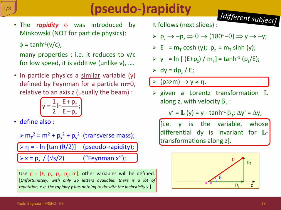
• The rapidity φ was introduced by Minkowski (NOT for particle physics):
φ = tanh-1(v/c), many properties : i.e. it reduces to v/c for low speed, it is additive (unlike v), ….
• In particle physics a similar variable (y) defined by Feynman for a particle m≠0, relative to an axis z (usually the beam) :
• define also :
mT2 = m2 + px
2 + py2 (transverse mass);
η = - ln [tan (θ/2)] (pseudo-rapidity);
x = pz / (√s/2) (“Feynman x”);
It follows (next slides) :
pz → −pz ⇒ θ → (180°−θ) ⇒ y → −y;
E = mT cosh (y); pz = mT sinh (y);
y = ln [ (E+pz) / mT] = tanh-1 (pz/E);
dy = dpz / E;
(p≫m) → y ≈ η.
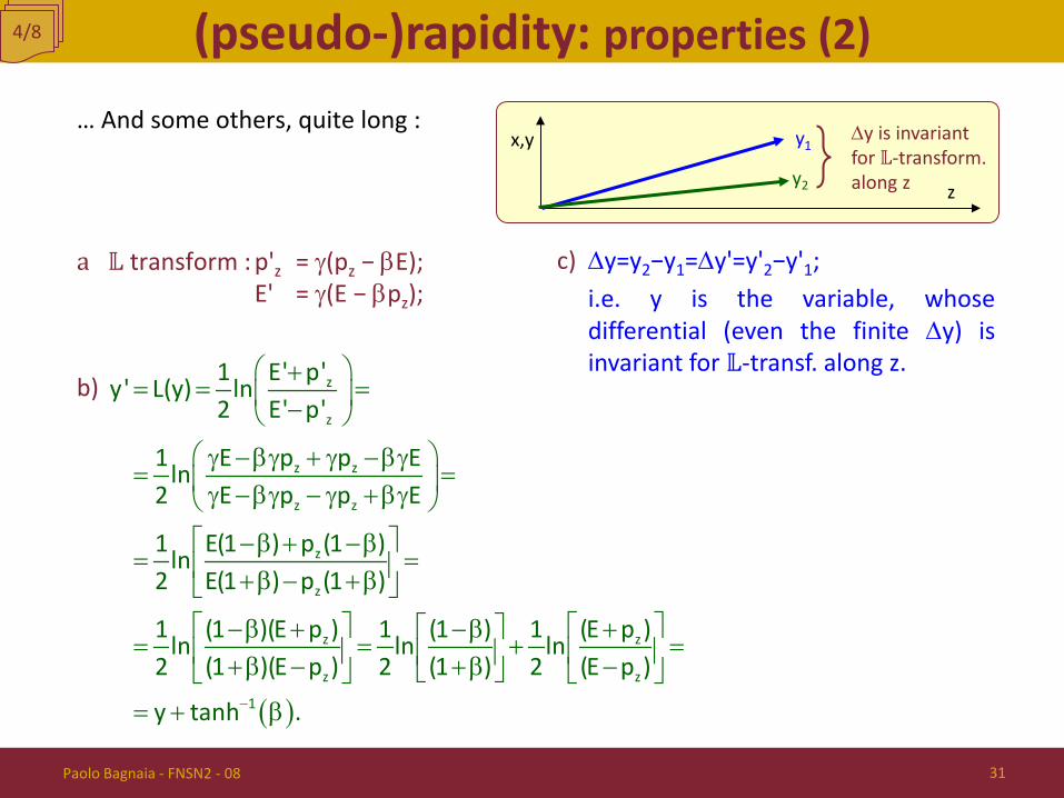
given a Lorentz transformation 𝕃 along z, with velocity βz :
y’ = 𝕃 (y) = y - tanh-1 βz; ∆y' = ∆y;
[i.e. y is the variable, whose differential dy is invariant for 𝕃-transformations along z].
(pseudo-)rapidity
Use p = [E, px, py, pz; m]; other variables will be defined. [Unfortunately, with only 26 letters available, there is a lot of repetition, e.g. the rapidity y has nothing to do with the inelasticity y.] z
pT p
θ pz
1/8
+=
−z
z
1 E py ln ;2 E p
Paolo Bagnaia - FNSN2 - 08 28
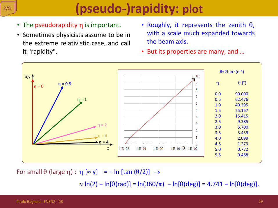
(pseudo-)rapidity: plot • The pseudorapidity η is important. • Sometimes physicists assume to be in
the extreme relativistic case, and call it "rapidity".
• Roughly, it represents the zenith θ, with a scale much expanded towards the beam axis.
• But its properties are many, and …
2/8
θ=2tan-1(e−η) η θ (°) 0.0 90.000 0.5 62.476 1.0 40.395 1.5 25.157 2.0 15.415 2.5 9.385 3.0 5.700 3.5 3.459 4.0 2.099 4.5 1.273 5.0 0.772 5.5 0.468
z
x,y
η = 0
η = 1
η = 4 η = 3
η = 0.5
For small θ (large η) : η [≈ y] = − ln [tan (θ/2)] →
≈ ln(2) − ln[θ(rad)] = ln(360/π) − ln[θ(deg)] = 4.741 − ln[θ(deg)].
Paolo Bagnaia - FNSN2 - 08 29
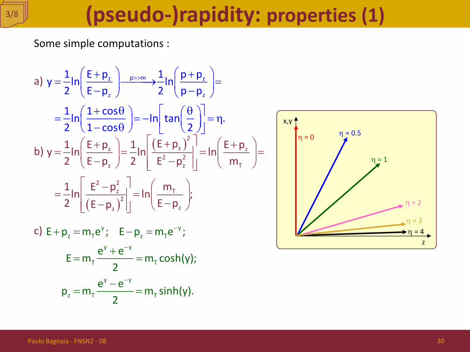
(pseudo-)rapidity: properties (1) Some simple computations :
a)
b)
c)
3/8
>> + += → = − −
+ θ θ = = − = η − θ
p mz z
z z
1 E p 1 p py ln ln2 E p 2 p p
1 1 cosln ln tan .2 1 cos 2
( )
( )
+ + += = = = − −
−= = −−
2zz z
2 2z z T
2 2z T
2zz
E p1 E p 1 E py ln ln ln2 E p 2 E p m
1 E p mln ln ;2 E pE p
z
x,y
η = 0
η = 1
η = 4 η = 3
η = 0.5
−
−
−
+ = − =
+= =
−= =
y yz T z T
y y
T T
y y
z T T
E p m e ; E p m e ;
e eE m m cosh(y);2
e ep m m sinh(y).2
Paolo Bagnaia - FNSN2 - 08 30
(pseudo-)rapidity: properties (2)
… And some others, quite long :
a) 𝕃 transform : p'z = γ(pz − βE); E' = γ(E − βpz);
b)
c) ∆y=y2−y1=∆y'=y'2−y'1; i.e. y is the variable, whose
differential (even the finite ∆y) is invariant for 𝕃-transf. along z.
z
x,y
y2
∆y is invariant for 𝕃-transform. along z
4/8
−
+= = = −
γ −βγ + γ −βγ= = γ −βγ − γ + βγ
−β + −β= = + β − + β
−β + −β += = + = + β − + β − = +
z
z
z z
z z
z
z
z z
z z
1
1 E' p'y' L(y) ln2 E' p'
1 E p p Eln2 E p p E
1 E(1 ) p (1 )ln2 E(1 ) p (1 )
1 (1 )(E p ) 1 (1 ) 1 (E p )ln ln ln2 (1 )(E p ) 2 (1 ) 2 (E p )
y tanh ( )β .
Paolo Bagnaia - FNSN2 - 08 31
(pseudo-)rapidity: properties (3) • Start from well-known math :
• Then :
• i.e. the differential dy = dpz / E = dE / pz at constant pT.
• Definition of the invariant cross section ["invariant" under 𝕃-transform. along z] :
5/8
= + +
= → =
2 2 2z T
z z z
z
E p p m ;p dp dp dEdE .
E E p
( ) ( )
( ) ( )
z z zz z2 2
z z z zz z
z z z z z z zz2 2
z z z
z z2 2
z
y y 1 E p 1 E p 1 E pdy dp dE dp dEp E 2 E p E p E pE p E p
1 E p E p E p E p E p p dpdp2 E p EE p E p
1 dp 2p2E2 E p
∂ ∂ − + += + = + + − = ∂ ∂ + − −− −
− − + + − − −= + = + − −
= − −
2 2z z z
z 2 2z z
1 dp E p dp dEp 2 .E 2 E p E E p
− = = = −
σ σ σ σ= = = ϕ π
3 3 2 3
2x y z T T T x y z
Ed d 1 d E'd .dp dp dp p dp d dy dp dy dp' dp' dp'
Paolo Bagnaia - FNSN2 - 08 32
+= −
z
z
1 E py ln2 E p

(pseudo-)rapidity: properties (4)
• [curiosity : an alternative way to show that y is invariant for 𝕃-transf. along z :
6/8
( )
z z
z
z z z zz z z z
z
z zz z
z z
p' (p E);E' (E p );
p' p' p dpdp' dp dE dp dE dpp E E
p dpdp 1 E p ;E E
dp' dpi.e. dy' dy].E' E
= γ −β = γ −β
∂ ∂= + = γ −βγ = γ −βγ =
∂ ∂
β γ = γ − = −β
= = =
Paolo Bagnaia - FNSN2 - 08 33
z
x,y
η = 0
η = 1
η = 4 η = 3
η = 0.5
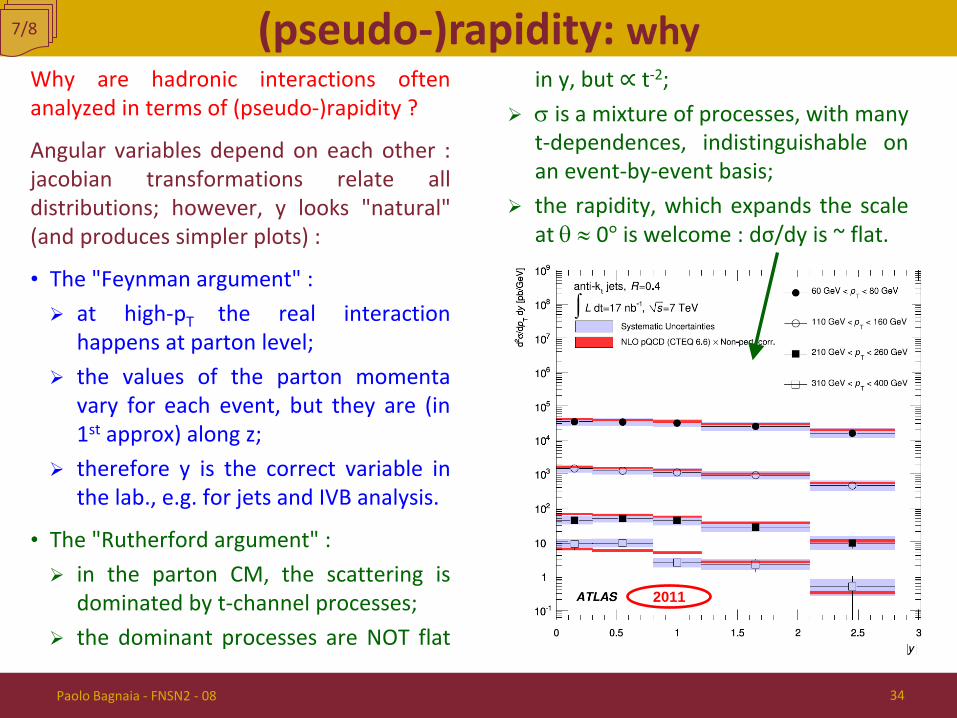
Why are hadronic interactions often analyzed in terms of (pseudo-)rapidity ?
Angular variables depend on each other : jacobian transformations relate all distributions; however, y looks "natural" (and produces simpler plots) :
• The "Feynman argument" : at high-pT the real interaction
happens at parton level; the values of the parton momenta
vary for each event, but they are (in 1st approx) along z;
therefore y is the correct variable in the lab., e.g. for jets and IVB analysis.
• The "Rutherford argument" : in the parton CM, the scattering is
dominated by t-channel processes; the dominant processes are NOT flat
in y, but ∝ t-2; σ is a mixture of processes, with many
t-dependences, indistinguishable on an event-by-event basis;
the rapidity, which expands the scale at θ ≈ 0° is welcome : dσ/dy is ~ flat.
(pseudo-)rapidity: why 7/8
2011
Paolo Bagnaia - FNSN2 - 08 34
(pseudo-)rapidity: how Why are soft hadronic interactions often analyzed in terms of (pseudo-)rapidity ? The phenomenology of low-pT : • [maybe reasons based on low-pT physics,
related to the invariant cross-section]; • the inclusive y distributions are ~ flat; • so, y is very handy for fast background
computations. Why is η used (almost) always, instead of y ? • y has important physical properties; • y is difficult to measure, since is a small
difference of two large quantities (E, pz); • η is an angle, experimentalist friendly; • worst : in the literature sometimes η is
given the properties of y [but it is ALMOST correct].
Instead, e+e− interactions, where partons (=e±) interact in the LAB at x=1, are usually analyzed in terms of cos θ.
8/8
Paolo Bagnaia - FNSN2 - 08 35
it means : jets are integrated between ±η; the resultant number is divided by 2η; we used η = 1, if I remember correctly.
How to do it ? "typical example" : a hard interaction studied in terms of d2σ/dpTdη|η=0.
Log s physics 1/8
• An intuitive toy-model, with surprisingly good results :
σtot(pp or p p) ≈ πR2 ≈ π (ℏc/mπ)2 = = π(197 MeV·fm / 140 MeV)2 = 62 mb.
• A limit ("Froissart bound") on the increase of cross-section for any pairs of particles, when √s increases : for any two particles (ab) [e.g. pp, pp] :
"at sufficiently high energies, the total cross-section for scattering on a given target [e.g . σ(pp) or σ(pp) cannot grow faster than ln2 s]".
• A theorem, based on quantum field theory (NOT on dynamical assumptions, i.e. valid for any type of interaction), knows as the "Pomeranchuk theorem" :
"at sufficiently high energies, the cross-section for scattering on a given target is the same for a particle and its antiparticle" [e.g. σ(p p) ≈ σ(pp)].
• The (unexpected) experimental behavior that indeed hadron cross-sections grow with √s, [∝ ln(s) or maybe ∝ ln2(s)], and that the “Pomeranchuk regime” is reached at accelerator energies.
↓
p (−) p
→∞
σ= σ
ab
sab
lim 1, for any two particles (a,b).
( )→∞
σ ≤ × 2abs
lim const ln s ,
Paolo Bagnaia - FNSN2 - 08 36
↓ • … gave rise (50 years ago) to much
excitement and phenomenological models of low pT hadronic interactions ("Regge poles", "Pomeron", "cylindrical phase space", ...).
• Then, no real breakthrough for many years …
Comments (very personal) : physics born many years ago ('50s +
CERN ISR), before the advent of QCD; poor conceptual foundations, but many
phenomenological successes; many mysteries remain (perhaps no
mystery, only complex many-body interactions, e.g. chemistry);
today the main motivation of the study is to predict, parameterize and filter the background. In the following, we will assume this
attitude.
The funny name "Log s physics" comes from the fact that, in low-pT processes, the evolution with s of many quantities is logarithmic; the reasons are not really understood (Froissart ?).
Log s physics: comments 2/8
Paolo Bagnaia - FNSN2 - 08 37
there are books with an extensive treatment of the subject; instead we summarize everything here.
p (−) p
Log s physics: pp 3/8
The data of pp are dashed, to show the similarity of the cross sections.
Paolo Bagnaia - FNSN2 - 08 38
1 b = 10-28 m2 = 10-24 cm2
1 mb = 10-31 m2 = 10-27 cm2
LHC
pp [Tevatron]
[SppS]
@1034
cm-2s -1 109
108
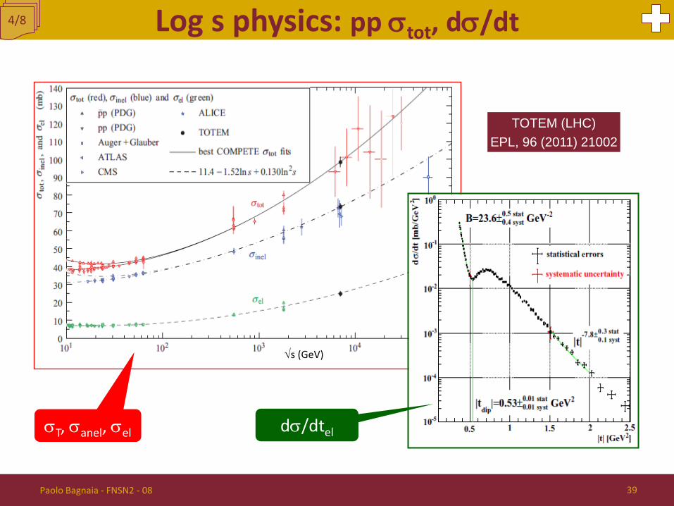
Log s physics: pp σtot, dσ/dt 4/8
σT, σanel, σel
TOTEM (LHC) EPL, 96 (2011) 21002
dσ/dtel
Paolo Bagnaia - FNSN2 - 08 39
√s (GeV)
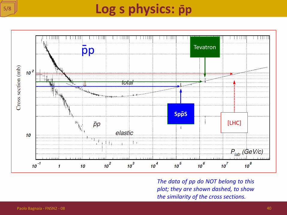
Log s physics: pp 5/8
pp
[LHC]
Tevatron
SppS
The data of pp do NOT belong to this plot; they are shown dashed, to show the similarity of the cross sections.
Paolo Bagnaia - FNSN2 - 08 40
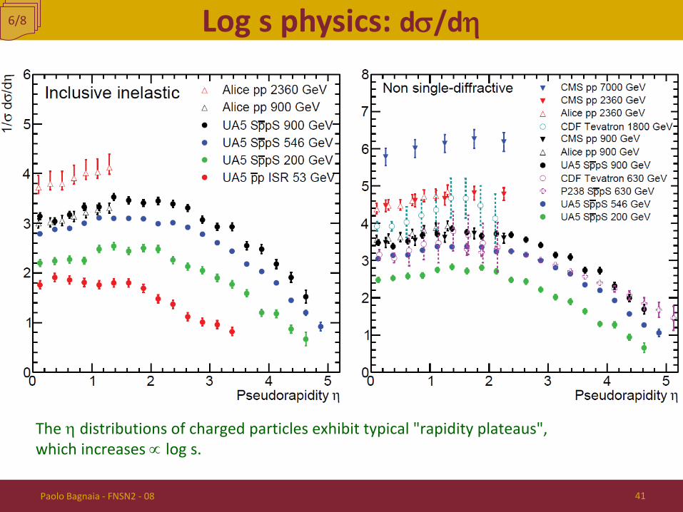
Log s physics: dσ/dη 6/8
The η distributions of charged particles exhibit typical "rapidity plateaus", which increases ∝ log s.
Paolo Bagnaia - FNSN2 - 08 41
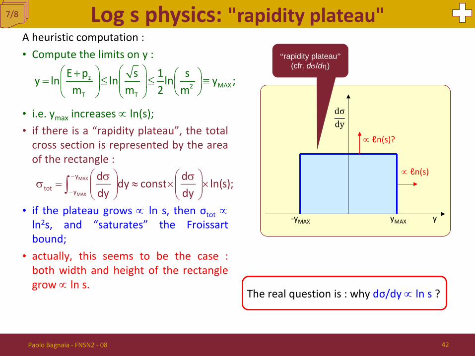
A heuristic computation : • Compute the limits on y :
• i.e. ymax increases ∝ ln(s); • if there is a “rapidity plateau”, the total
cross section is represented by the area of the rectangle :
• if the plateau grows ∝ ln s, then σtot ∝
ln2s, and “saturates” the Froissart bound;
• actually, this seems to be the case : both width and height of the rectangle grow ∝ ln s.
The real question is : why dσ/dy ∝ ln s ?
Log s physics: "rapidity plateau" 7/8
y -yMAX yMAX
∝ ℓn(s)?
∝ ℓn(s)
dσdy
“rapidity plateau” (cfr. dσ/dη) + = ≤ ≤ ≡
zMAX2
T T
E p s 1 sy ln ln ln y ;m m 2 m
MAX
MAX
y
tot y
d ddy const ln(s);dy dy
−
−
σ σ σ = ≈ × ×
∫
Paolo Bagnaia - FNSN2 - 08 42
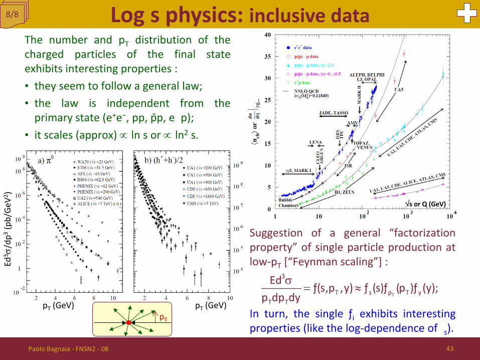
Log s physics: inclusive data 8/8
σ= ≈
T
3
T s p T yT T
Ed ƒ(s,p ,y) ƒ (s)ƒ (p )ƒ (y);p dp dy
Paolo Bagnaia - FNSN2 - 08 43
The number and pT distribution of the charged particles of the final state exhibits interesting properties : • they seem to follow a general law; • the law is independent from the
primary state (e+e−, pp, p p, e±p); • it scales (approx) ∝ ln s or ∝ ln2 s.
Suggestion of a general “factorization property” of single particle production at low-pT [“Feynman scaling”] :
In turn, the single ƒi exhibits interesting properties (like the log-dependence of ƒs).
√s or Q (GeV)
pT (GeV)
Ed3 σ
/dp3 (
pb/G
eV2 )
pT (GeV) pT
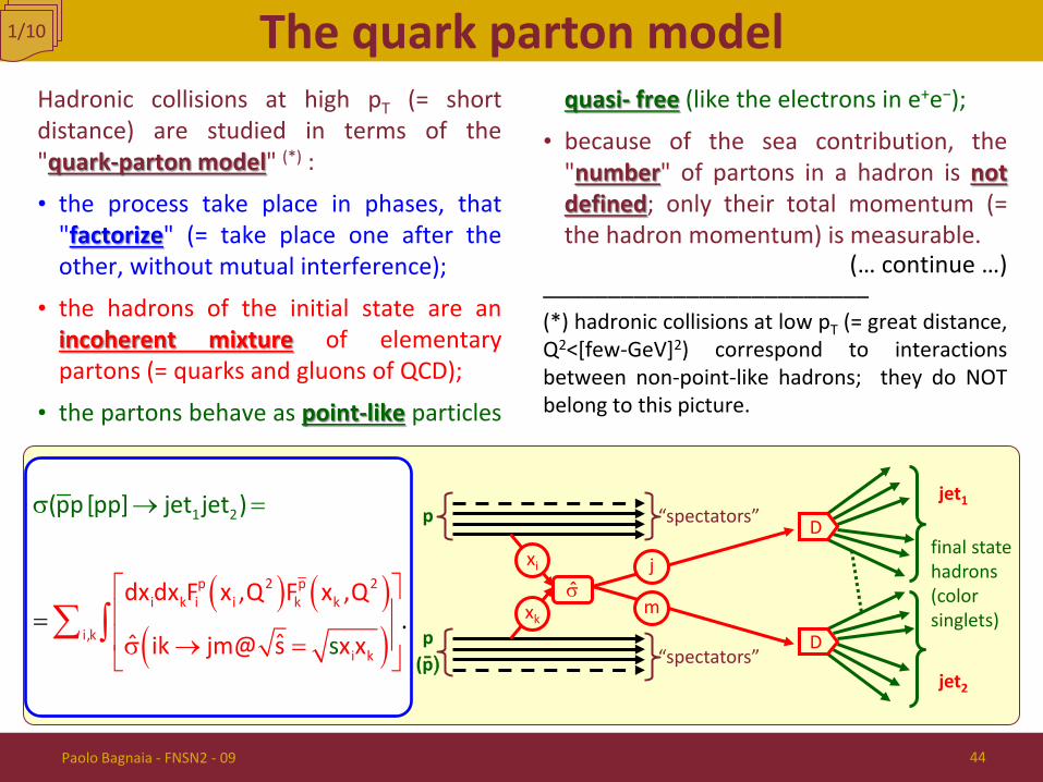
Hadronic collisions at high pT (= short distance) are studied in terms of the "quark-parton model" (*) :
• the process take place in phases, that "factorize" (= take place one after the other, without mutual interference);
• the hadrons of the initial state are an incoherent mixture of elementary partons (= quarks and gluons of QCD);
• the partons behave as point-like particles
quasi- free (like the electrons in e+e−);
• because of the sea contribution, the "number" of partons in a hadron is not defined; only their total momentum (= the hadron momentum) is measurable.
(… continue …) _________________________ (*) hadronic collisions at low pT (= great distance, Q2<[few-GeV]2) correspond to interactions between non-point-like hadrons; they do NOT belong to this picture.
The quark parton model 1/10
p
p (p)
“spectators”
“spectators”
xi
xk σ
final state hadrons (color singlets)
jet1
jet2
j
m
D
D
( ) ( )( )
σ → =
→
=
=
σ
∑ ∫p 2 p 2
i k i i k k
i,k
1 2
i k
dx dx F x ,Q F x ,Q
ˆˆ ik jm@
(pp [pp
s x x
] jet jet )
s.
Paolo Bagnaia - FNSN2 - 09 44
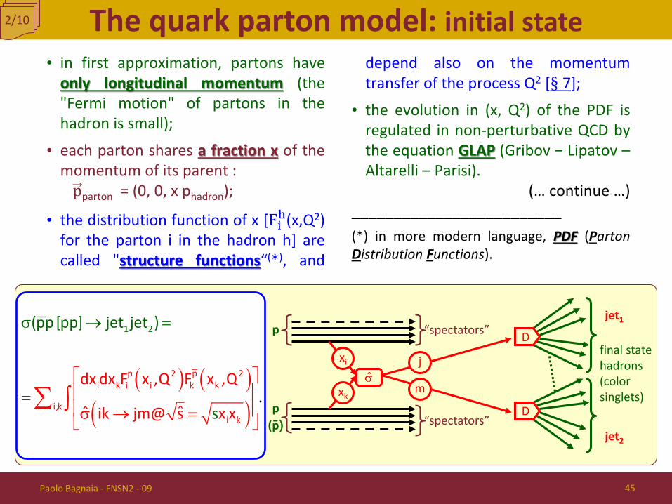
The quark parton model: initial state 2/10
• in first approximation, partons have only longitudinal momentum (the "Fermi motion" of partons in the hadron is small);
• each parton shares a fraction x of the momentum of its parent :
pparton = (0, 0, x phadron);
• the distribution function of x [Fih(x,Q2) for the parton i in the hadron h] are called "structure functions“(*), and
depend also on the momentum transfer of the process Q2 [§ 7];
• the evolution in (x, Q2) of the PDF is regulated in non-perturbative QCD by the equation GLAP (Gribov − Lipatov – Altarelli – Parisi).
(… continue …) _________________________ (*) in more modern language, PDF (Parton Distribution Functions).
Paolo Bagnaia - FNSN2 - 09 45
p
p (p)
“spectators”
“spectators”
xi
xk σ
final state hadrons (color singlets)
jet1
jet2
j
m
D
D
( ) ( )( )
σ → =
→
=
=
σ
∑ ∫p 2 p 2
i k i i k k
i,k
1 2
i k
dx dx F x ,Q F x ,Q
ˆˆ ik jm@
(pp [pp
s x x
] jet jet )
s.
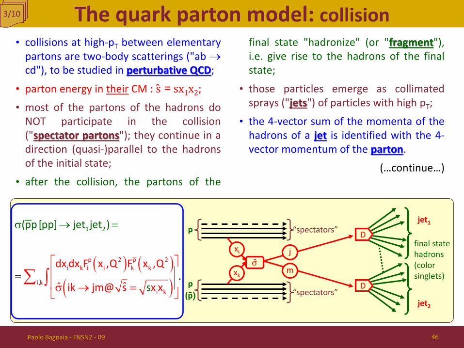
The quark parton model: collision 3/10
• collisions at high-pT between elementary partons are two-body scatterings ("ab → cd"), to be studied in perturbative QCD;
• parton energy in their CM : s = sx1x2;
• most of the partons of the hadrons do NOT participate in the collision ("spectator partons"); they continue in a direction (quasi-)parallel to the hadrons of the initial state;
• after the collision, the partons of the
final state "hadronize" (or "fragment"), i.e. give rise to the hadrons of the final state;
• those particles emerge as collimated sprays ("jets") of particles with high pT;
• the 4-vector sum of the momenta of the hadrons of a jet is identified with the 4-vector momentum of the parton.
(…continue…)
Paolo Bagnaia - FNSN2 - 09 46
p
p (p)
“spectators”
“spectators”
xi
xk σ
final state hadrons (color singlets)
jet1
jet2
j
m
D
D
( ) ( )( )
σ → =
→
=
=
σ
∑ ∫p 2 p 2
i k i i k k
i,k
1 2
i k
dx dx F x ,Q F x ,Q
ˆˆ ik jm@
(pp [pp
s x x
] jet jet )
s.

The quark parton model: fragmentation 4/10
• The distributions of the final state hadrons are called "fragmentation functions";
• they are functions [Dph(z,Q2)] of the
variable z = phadron / pparton, which defines the distribution of hadron "h" in a jet from parton "p";
• they do NOT depend, to a good approximation, neither on the initial
state, nor on the elementary collision, but only on the final state parton and the value of Q2;
• however, unlike the partons of the elementary collision, the hadrons are color singlets; therefore in the process of fragmentation particles of different jets must interact.
Paolo Bagnaia - FNSN2 - 09 47
p
p (p)
“spectators”
“spectators”
xi
xk σ
final state hadrons (color singlets)
jet1
jet2
j
m
D
D
( ) ( )( )
σ → =
→
=
=
σ
∑ ∫p 2 p 2
i k i i k k
i,k
1 2
i k
dx dx F x ,Q F x ,Q
ˆˆ ik jm@
(pp [pp
s x x
] jet jet )
s.
The quark parton model: electroweak 5/10
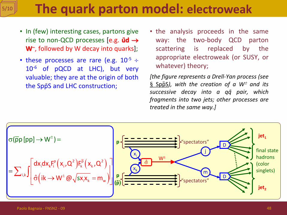
• In (few) interesting cases, partons give rise to non-QCD processes [e.g. ud → W−, followed by W decay into quarks];
• these processes are rare (e.g. 10-5 ÷ 10-6 of pQCD at LHC), but very valuable; they are at the origin of both the Spp S and LHC construction;
• the analysis proceeds in the same way: the two-body QCD parton scattering is replaced by the appropriate electroweak (or SUSY, or whatever) theory;
[the figure represents a Drell-Yan process (see § SppS), with the creation of a W± and its successive decay into a qq pair, which fragments into two jets; other processes are treated in the same way.]
Paolo Bagnaia - FNSN2 - 09 48
p
p (p)
“spectators”
“spectators”
xi
xk
final state hadrons (color singlets)
jet1
jet2
j D
D
( ) ( )( )
±
±=
σ → =
σ =
→
∑ ∫
p 2 p 2i k i i k k
i,ki k w
dx dx F x ,Q F x ,Q
ˆ ik W @ x x
(pp [pp W )
m
]
sm
σ W±
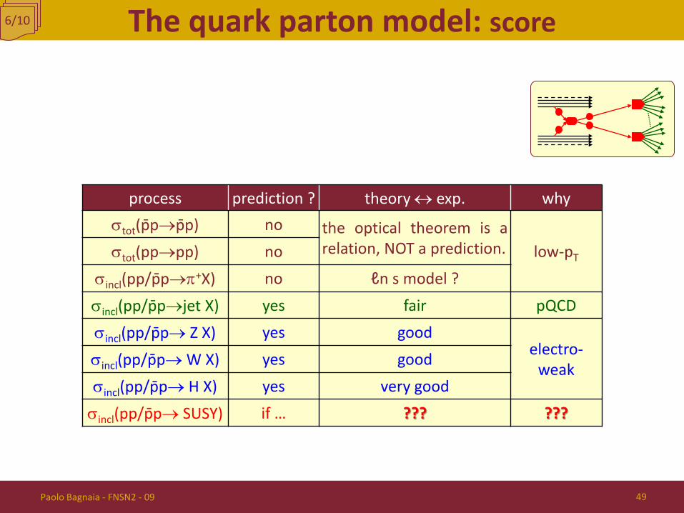
The quark parton model: score 6/10
process prediction ? theory ↔ exp. why σtot(p p→p p) no the optical theorem is a
relation, NOT a prediction. low-pT σtot(pp→pp) no
σincl(pp/p p→π+X) no ℓn s model ?
σincl(pp/p p→jet X) yes fair pQCD
σincl(pp/p p→ Z X) yes good electro-
weak σincl(pp/p p→ W X) yes good
σincl(pp/p p→ H X) yes very good
σincl(pp/p p→ SUSY) if … ??? ???
Paolo Bagnaia - FNSN2 - 09 49
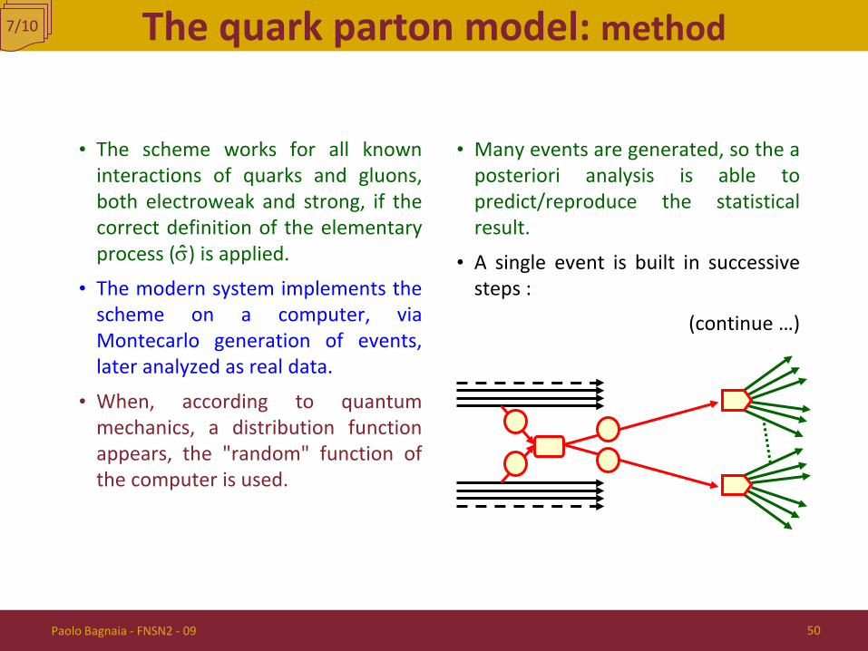
The quark parton model: method 7/10
• The scheme works for all known interactions of quarks and gluons, both electroweak and strong, if the correct definition of the elementary process (σ) is applied.
• The modern system implements the scheme on a computer, via Montecarlo generation of events, later analyzed as real data.
• When, according to quantum mechanics, a distribution function appears, the "random" function of the computer is used.
• Many events are generated, so the a posteriori analysis is able to predict/reproduce the statistical result.
• A single event is built in successive steps :
(continue …)
Paolo Bagnaia - FNSN2 - 09 50
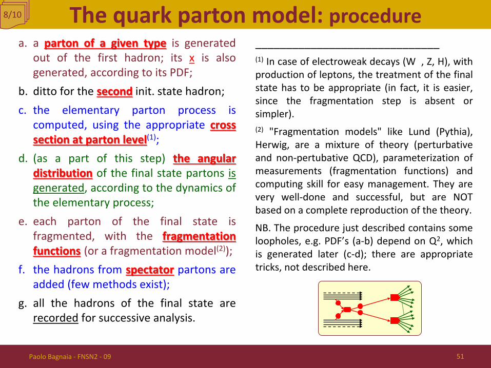
a. a parton of a given type is generated out of the first hadron; its x is also generated, according to its PDF;
b. ditto for the second init. state hadron; c. the elementary parton process is
computed, using the appropriate cross section at parton level(1);
d. (as a part of this step) the angular distribution of the final state partons is generated, according to the dynamics of the elementary process;
e. each parton of the final state is fragmented, with the fragmentation functions (or a fragmentation model(2));
f. the hadrons from spectator partons are added (few methods exist);
g. all the hadrons of the final state are recorded for successive analysis.
______________________________ (1) In case of electroweak decays (W±, Z, H), with production of leptons, the treatment of the final state has to be appropriate (in fact, it is easier, since the fragmentation step is absent or simpler). (2) "Fragmentation models" like Lund (Pythia), Herwig, are a mixture of theory (perturbative and non-pertubative QCD), parameterization of measurements (fragmentation functions) and computing skill for easy management. They are very well-done and successful, but are NOT based on a complete reproduction of the theory.
NB. The procedure just described contains some loopholes, e.g. PDF’s (a-b) depend on Q2, which is generated later (c-d); there are appropriate tricks, not described here.
The quark parton model: procedure 8/10
Paolo Bagnaia - FNSN2 - 09 51
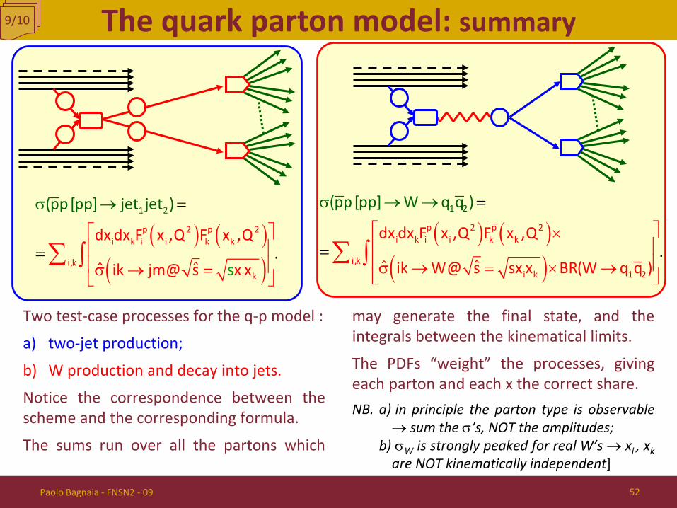
Two test-case processes for the q-p model :
a) two-jet production;
b) W production and decay into jets.
Notice the correspondence between the scheme and the corresponding formula.
The sums run over all the partons which
may generate the final state, and the integrals between the kinematical limits.
The PDFs “weight” the processes, giving each parton and each x the correct share. NB. a) in principle the parton type is observable
→ sum the σ’s, NOT the amplitudes; b) σW is strongly peaked for real W’s → xi , xk
are NOT kinematically independent]
The quark parton model: summary 9/10
( ) ( )( )
σ → =
→
=
=
σ
∑ ∫p 2 p 2
i k i i k k
i,k
1 2
i k
dx dx F x ,Q F x ,Q
ˆˆ ik jm@
(pp [pp
s x x
] jet jet )
s.
( ) ( )( )
×
σ
σ → =
→
→
→
=
=×
∑ ∫p 2 p 2
i k i i k k
i,ki k 1 2
1 2
dx dx F x ,Q F x ,Q
ˆˆ
(p
ik W@ s sx x B
p [pp] W q q
q
)
R(W q ).
Paolo Bagnaia - FNSN2 - 09 52
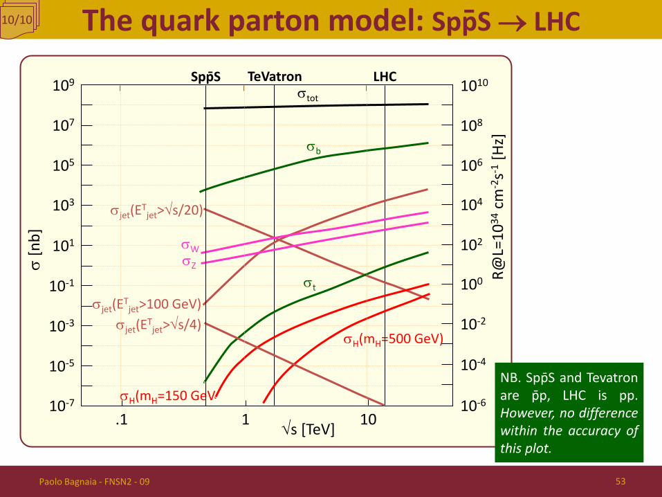
The quark parton model: SppS → LHC 10/10
Paolo Bagnaia - FNSN2 - 09 53
√s [TeV]
σH(mH=500 GeV)
10-7
10-5
10-3
10-1
101
103
105
107
109
10-6
10-4
10-2
100
102
104
106
108
1010 σtot
σb
σjet(ETjet>√s/20)
σW σZ
σjet(ETjet>100 GeV)
σt
σjet(ETjet>√s/4)
σH(mH=150 GeV
TeVatron LHC
σ [n
b]
R@L=
1034
cm
-2s-1
[Hz]
.1 1 10
SppS
NB. SppS and Tevatron are pp, LHC is pp. However, no difference within the accuracy of this plot.
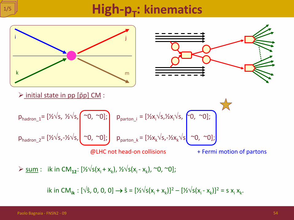
High-pT: kinematics 1/5
initial state in pp [pp] CM : phadron_1= [½√s, ½√s, ~0, ~0]; pparton_i = [½xi√s,½xi√s, ~0, ~0]; phadron_2= [½√s, -½√s, ~0, ~0]; pparton_k = [½xk√s,-½xk√s, ~0, ~0]; sum : ik in CM12 : [½√s(xi + xk), ½√s(xi - xk), ~0, ~0]; ik in CMik : [√s, 0, 0, 0] → s = [½√s(xi + xk)]2 – [½√s(xi - xk)]2 = s xi xk.
i
m
j
k
+ Fermi motion of partons @LHC not head-on collisions
Paolo Bagnaia - FNSN2 - 09 54
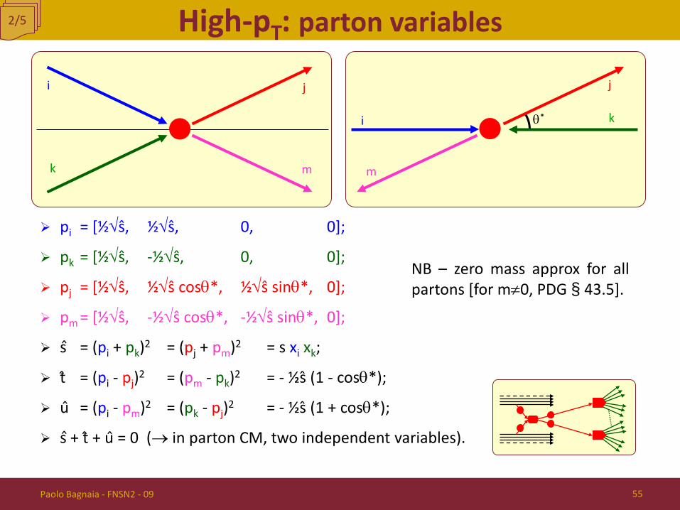
High-pT: parton variables 2/5
pi = [½√ŝ, ½√ŝ, 0, 0];
pk = [½√ŝ, -½√ŝ, 0, 0];
pj = [½√ŝ, ½√ŝ cosθ*, ½√ŝ sinθ*, 0];
pm = [½√ŝ, -½√ŝ cosθ*, -½√ŝ sinθ*, 0];
s = (pi + pk)2 = (pj + pm)2 = s xi xk;
t = (pi - pj)2 = (pm - pk)2 = - ½s (1 - cosθ*);
u = (pi - pm)2 = (pk - pj)2 = - ½s (1 + cosθ*);
s + t + u = 0 (→ in parton CM, two independent variables).
i
m
j
k
i
m
j
k θ*
NB – zero mass approx for all partons [for m≠0, PDG § 43.5].
Paolo Bagnaia - FNSN2 - 09 55
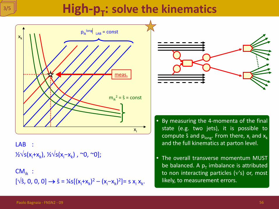
High-pT: solve the kinematics 3/5
xi
xk pik
longLAB = const
mik2 = s = const
meas.
• By measuring the 4-momenta of the final state (e.g. two jets), it is possible to compute s and plong. From there, xi and xk and the full kinematics at parton level.
• The overall transverse momentum MUST be balanced. A pT imbalance is attributed to non interacting particles (ν's) or, most likely, to measurement errors.
Paolo Bagnaia - FNSN2 - 09 56
CMik : [√s, 0, 0, 0] → ŝ = ¼s[(xi+xk)2 – (xi−xk)2]= s xi xk.
LAB : ½√s(xi+xk), ½√s(xi−xk) , ~0, ~0];
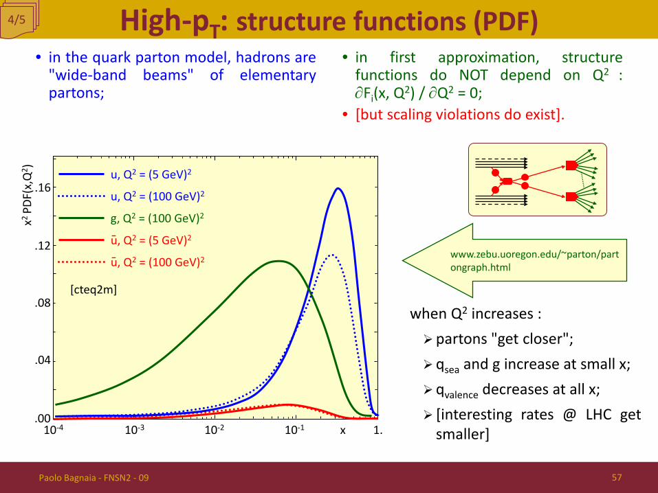
High-pT: structure functions (PDF) • in the quark parton model, hadrons are
"wide-band beams" of elementary partons;
• in first approximation, structure functions do NOT depend on Q2 : ∂Fi(x, Q2) / ∂Q2 = 0;
• [but scaling violations do exist].
4/5
u, Q2 = (5 GeV)2
.00
.08
10-4 10-3 10-2 10-1 1.
.04
.12
.16
[cteq2m]
u, Q2 = (100 GeV)2
g, Q2 = (100 GeV)2
u, Q2 = (5 GeV)2
u, Q2 = (100 GeV)2
x
x2 PD
F(x,
Q2 )
when Q2 increases : partons "get closer"; qsea and g increase at small x; qvalence decreases at all x; [interesting rates @ LHC get
smaller]
www.zebu.uoregon.edu/~parton/partongraph.html
Paolo Bagnaia - FNSN2 - 09 57

Jet reconstruction algorithm (one of many many many …)
hadrons
High-pT: partons → jets • reconstruct the jets via an algorithm : simple clustering of nearby calo cells; cone algo. (see fig) with fixed ∆R
(very popular ∆R2 = ∆φ2 + ∆η2 = 1); "Durham" anti-Kt …
• more refined cooking (split, sum, …) • reconstruct 4-momentum : pjet=Σphadrons; Ejet=ΣEhadrons; • [notice that the above definition gives jets a
mass ≠ 0, generally much larger than the tiny parton mass → more cooking …]
• identify jet → parton and play with its 4-momentum;
• check the manipulations with known cases (W±, Z → jets) and montecarlo.
5/5
calo cells
Paolo Bagnaia - FNSN2 - 09 58
CDF – Z→ e+e− + jets
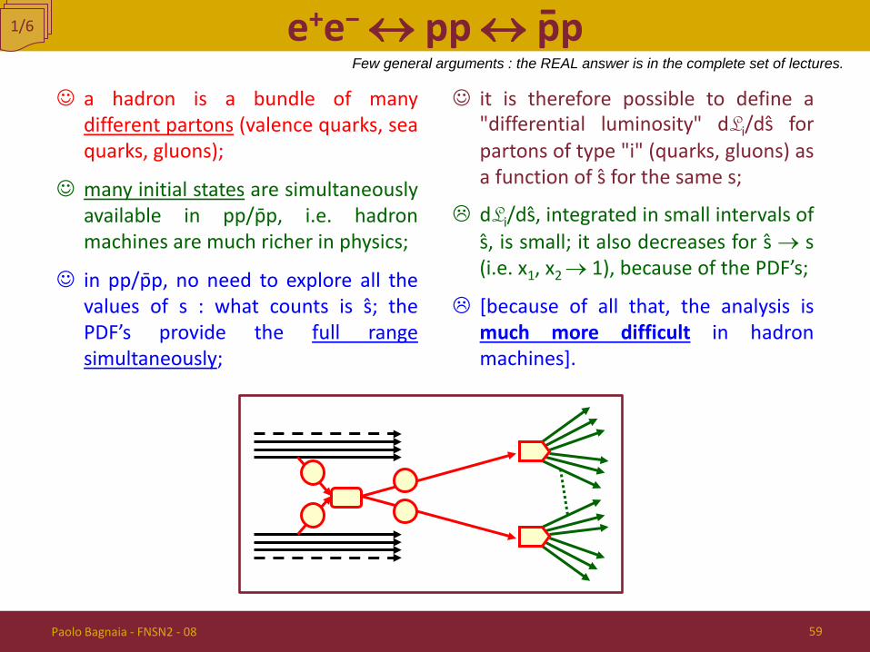
e+e− ↔ pp ↔ pp a hadron is a bundle of many
different partons (valence quarks, sea quarks, gluons);
many initial states are simultaneously available in pp/pp, i.e. hadron machines are much richer in physics;
in pp/pp, no need to explore all the values of s : what counts is s; the PDF’s provide the full range simultaneously;
it is therefore possible to define a "differential luminosity" dLi/ds for partons of type "i" (quarks, gluons) as a function of s for the same s;
dLi/ds, integrated in small intervals of s, is small; it also decreases for s → s (i.e. x1, x2 → 1), because of the PDF’s;
[because of all that, the analysis is much more difficult in hadron machines].
1/6
Paolo Bagnaia - FNSN2 - 08 59
Few general arguments : the REAL answer is in the complete set of lectures.

e+e− ↔ pp ↔ pp : soft vs hard collisions • ex. : σ(LEP II, e+e−→ hadr., √s = 200 GeV) ≈ 100 pb;
σ(LHC, pp → total, √s = 14 TeV) ≈ 100 mb;
σ(LHC, pp → jet X, ETjet > 250 GeV) ≈ 100 nb.
2/6
~ 1 ÷ 109 ÷ 103
!!!
• nucleons, when coherent, are "one billion times" larger than electrons;
• however, when individual partons have to play, they are only "1,000 times" (the actual number depends on Q2) larger;
• the factor 1,000 is mainly due to the strength of the coupling (αs ↔ αem).
Paolo Bagnaia - FNSN2 - 08 60
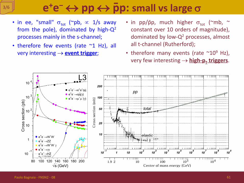
e+e− ↔ pp ↔ pp: small vs large σ 3/6
• in ee, "small" σtot (~pb, ∝ 1/s away from the pole), dominated by high-Q2 processes mainly in the s-channel;
• therefore few events (rate ~1 Hz), all very interesting → event trigger;
• in pp/pp, much higher σtot (~mb, ~ constant over 10 orders of magnitude), dominated by low-Q2 processes, almost all t-channel (Rutherford);
• therefore many events (rate ~109 Hz), very few interesting → high-pT triggers.
Paolo Bagnaia - FNSN2 - 08 61
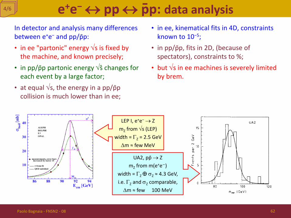
e+e− ↔ pp ↔ pp: data analysis In detector and analysis many differences between e+e− and pp/pp: • in ee "partonic" energy √s is fixed by
the machine, and known precisely; • in pp/pp partonic energy √s changes for
each event by a large factor; • at equal √s, the energy in a pp/pp
collision is much lower than in ee;
• in ee, kinematical fits in 4D, constraints known to 10−5;
• in pp/pp, fits in 2D, (because of spectators), constraints to %;
• but √s in ee machines is severely limited by brem.
4/6
LEP I, e+e− → Z mZ from √s (LEP)
width = ΓZ = 2.5 GeV ∆m ≈ few MeV
UA2, pp → Z mZ from m(e+e−)
width = ΓZ ⊕ σZ ≈ 4.3 GeV, i.e. ΓZ and σZ comparable,
∆m ≈ few × 100 MeV
Paolo Bagnaia - FNSN2 - 08 62
e+e− ↔ pp ↔ pp: a personal conclusion In a given moment, with similar technology (and resources, don't forget) : A pp/p p machine : • needs a smaller ring (because of brem); • more difficult to build (both the
magnets and the detectors); • (much) higher √s and (fairly) higher √s; • more analysis, but higher systematics; • larger variety of both initial and final
states (not only vacuum q.n.); Therefore [imho, but largely shared]: (ee) and (pp/pp) complementary, NOT
competitive; (pp/pp) an exploratory machine, for
first generation experiments; (ee) a "second generation" machine,
for systematics and consolidation (and possible surprises in the details);
This has been the CERN strategy in the last half a century : 1. (pp/p p) (re-using an old machine); 2. civil engineering for a new ring (the
long and expensive step); 3. (ee) in the new ring; 4. [back to step (1), restart the cycle]. It happens that, e.g., the value of √s in step (3) is similar to seff in step (4/1) [e.g. both the Spp S and LEP had W± and Z as the main purpose. The "luminosity frontier" (Babar, Daφne, …) is a different approach : a dedicated machine for few (even only one) purposes, especially optimized wrt intensity and systematics, for (a) very important (single) measurement(s).
Q. Does the Higgs search fit with the scheme?
5/6
Paolo Bagnaia - FNSN2 - 08 63

e+e− ↔ pp ↔ pp: matter vs antimatter Last question : pp ↔ p p ?
• pp has major problems : it needs two independent magnet
rings; at the same √s, the effective √s is
smaller for qq channels (valence-sea instead of valence-valence);
• however, there is a larger problem : antiprotons do NOT exist in
nature (at least in our proximity); therefore they have to be "built".
starting from pp collisions; they are scarce, and have an
incredible "price" (in the Spp S, one good p / 3×10⁵ pp collisions);
they have to be cooled and stored (AA, stochastic cooling, van der Meer);
the resultant luminosity is small (in 1983, the golden year, L(SppS) < 1030 cm-2s-1);
• Therefore, in spite of all the successes of the p p machines, both at CERN and Fermilab, the quest for higher energies and (consequently) higher luminosities makes the pp option really superior for present and future colliders.
• The pp option will probably be reserved for dedicated single-task machines at sub-TeV energy.
6/6
Paolo Bagnaia - FNSN2 - 08 64

References
1. e.g. [BJ, 14];
2. for the results, see next 3 chapters;
3. accelerator physics : [BJ, 2], [Povh, appendix];
4. better accelerator physics : Ed. Wilson, An introduction to particle accelerators.
Paolo Bagnaia - FNSN2 - 08 65
God the Geometer, Frontispiece of Bible Moralisee Codex Vindobonensis 2554 (French, ca. 1250) [Österreichische Nationalbibliothek]

End of chapter 8
End
Paolo Bagnaia - FNSN2 - 08 66