Embed Size (px)
Citation preview
Gil-Jin Jang @ KNU
영상인식을위한 TensorFlow 공개도구사용법및의료영상에의응용
한국광학회튜토리얼
2019년 2월 22일
장길진 Gil-Jin Jang
경북대학교전자공학부
2/22/2019TensorFlow 공개도구사용법및의료영상응용 1
Gil-Jin Jang @ KNU
용어 정의
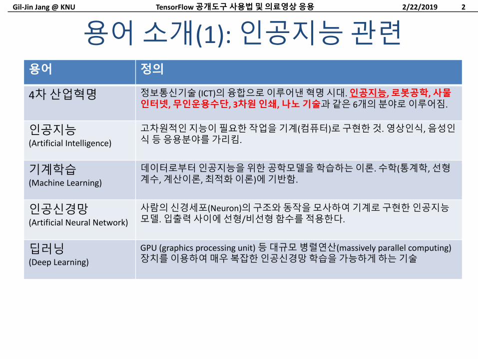
4차산업혁명 정보통신기술 (ICT)의융합으로이루어낸혁명시대. 인공지능, 로봇공학, 사물인터넷, 무인운용수단, 3차원인쇄, 나노기술과같은 6개의분야로이루어짐.
인공지능(Artificial Intelligence)
고차원적인지능이필요한작업을기계(컴퓨터)로구현한것. 영상인식, 음성인식등응용분야를가리킴.
기계학습(Machine Learning)
데이터로부터인공지능을위한공학모델을학습하는이론.수학(통계학, 선형계수, 계산이론, 최적화이론)에기반함.
인공신경망(Artificial Neural Network)
사람의신경세포(Neuron)의구조와동작을모사하여기계로구현한인공지능모델. 입출력사이에선형/비선형함수를적용한다.
딥러닝(Deep Learning)
GPU (graphics processing unit) 등대규모병렬연산(massively parallel computing)장치를이용하여매우복잡한인공신경망학습을가능하게하는기술
용어소개(1): 인공지능관련
2/22/2019TensorFlow 공개도구사용법및의료영상응용 2
Gil-Jin Jang @ KNU
용어 정의
왓슨온콜로지(Watson for Oncology)
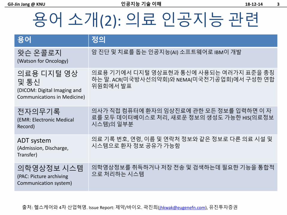
암진단및치료를돕는인공지능(AI) 소프트웨어로 IBM이개발
의료용디지털영상및통신(DICOM: Digital Imaging and Communications in Medicine)
의료용기기에서디지털영상표현과통신에사용되는여러가지표준을총칭하는말. ACR(미국방사선의약회)와 NEMA(미국전기공업회)에서구성한연합위원회에서발표
전자의무기록(EMR: Electronic Medical Record)
의사가직접컴퓨터에환자의임상진료에관한모든정보를입력하면이자료를모두데이터베이스로처리, 새로운정보의생성도가능한 HIS(의료정보시스템)의일부분
ADT system(Admission, Discharge, Transfer)
의료기록번호, 연령, 이름및연락처정보와같은정보로다른의료시설및시스템으로환자정보공유가가능함
의학영상정보시스템(PAC: Picture archiving Communication system)
의학영상정보를취득하거나저장전송및검색하는데필요한기능을통합적으로처리하는시스템
용어소개(2): 의료인공지능관련
18-12-14인공지능기술이해 3
출처: 헬스케어와 4차산업혁명. Issue Report: 제약/바이오. 곽진희([email protected]), 유진투자증권
Gil-Jin Jang @ KNU
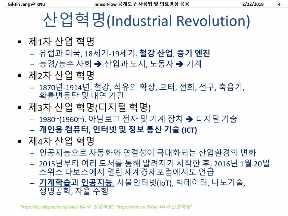
제1차산업혁명– 유럽과미국, 18세기-19세기. 철강산업, 증기엔진
– 농경/농촌사회산업과도시, 노동자기계
제2차산업혁명– 1870년-1914년. 철강, 석유의확장, 모터, 전화, 전구, 축음기, 확률변동탄및내연기관
제3차산업혁명(디지털혁명)– 1980~(1960~). 아날로그전자및기계장치디지털기술
– 개인용컴퓨터, 인터넷및정보통신기술 (ICT)
제4차산업혁명– 인공지능으로자동화와연결성이극대화되는산업환경의변화
– 2015년부터여러도서를통해알려지기시작한후, 2016년 1월 20일스위스다보스에서열린세계경제포럼에서도언급
– 기계학습과인공지능, 사물인터넷(IoT), 빅데이터, 나노기술, 생명공학, 자율주행
산업혁명(Industrial Revolution)
2/22/2019TensorFlow 공개도구사용법및의료영상응용 4
“http://ko.wikipedia.org/wiki/제4차_산업혁명”, “http://namu.wiki/w/제4차산업혁명”
Gil-Jin Jang @ KNU
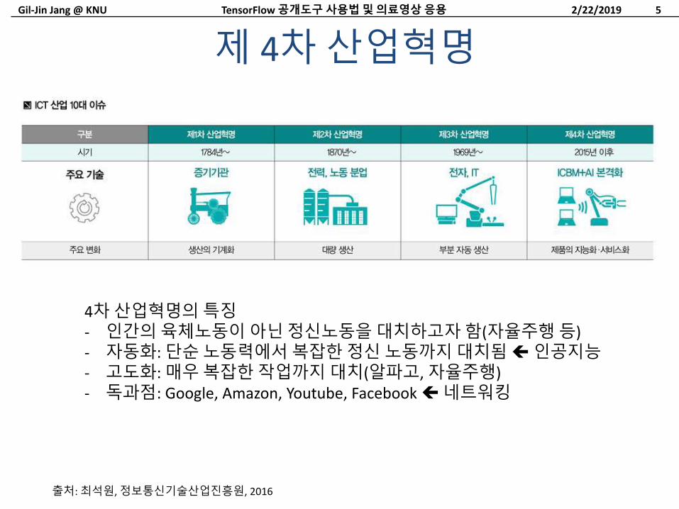
제 4차산업혁명
2/22/2019TensorFlow 공개도구사용법및의료영상응용 5
출처: 최석원, 정보통신기술산업진흥원, 2016
4차산업혁명의특징- 인간의육체노동이아닌정신노동을대치하고자함(자율주행등)- 자동화: 단순노동력에서복잡한정신노동까지대치됨인공지능- 고도화: 매우복잡한작업까지대치(알파고, 자율주행)- 독과점: Google, Amazon, Youtube, Facebook 네트워킹
Gil-Jin Jang @ KNU
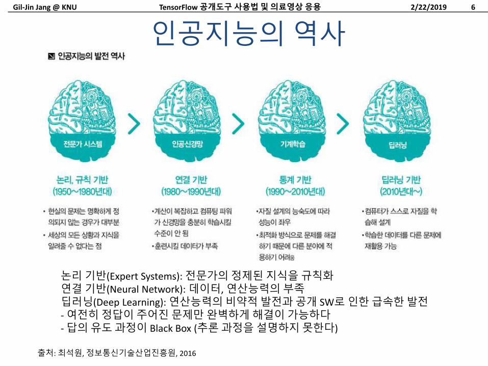
인공지능의역사
2/22/2019TensorFlow 공개도구사용법및의료영상응용 6
출처: 최석원, 정보통신기술산업진흥원, 2016
논리기반(Expert Systems): 전문가의정제된지식을규칙화연결기반(Neural Network): 데이터, 연산능력의부족딥러닝(Deep Learning): 연산능력의비약적발전과공개 SW로인한급속한발전- 여전히정답이주어진문제만완벽하게해결이가능하다- 답의유도과정이 Black Box (추론과정을설명하지못한다)
Gil-Jin Jang @ KNU
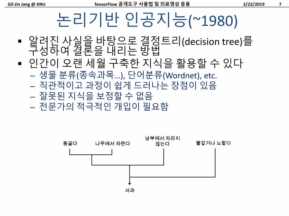
알려진사실을바탕으로결정트리(decision tree)를구성하여결론을내리는방법
인간이오랜세월구축한지식을활용할수있다– 생물분류(종속과목…), 단어분류(Wordnet), etc.– 직관적이고과정이쉽게드러나는장점이있음– 잘못된지식을보정할수없음– 전문가의적극적인개입이필요함
논리기반인공지능(~1980)
2/22/2019TensorFlow 공개도구사용법및의료영상응용 7
Gil-Jin Jang @ KNU
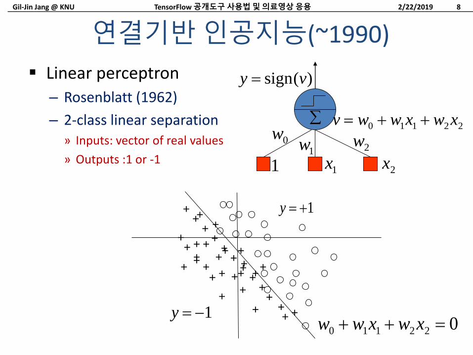
연결기반인공지능(~1990)
Linear perceptron
– Rosenblatt (1962)
– 2-class linear separation» Inputs: vector of real values
» Outputs :1 or -1
2/22/2019TensorFlow 공개도구사용법및의료영상응용 8
022110 xwxww
++++
++
++
++ + +
++ +
+
+++
++
+
++
++
+ ++
++
+
+
+
+
+
1y
1y
1x 2x1
0w1w 2w
22110 xwxwwv
)(sign vy
Gil-Jin Jang @ KNU
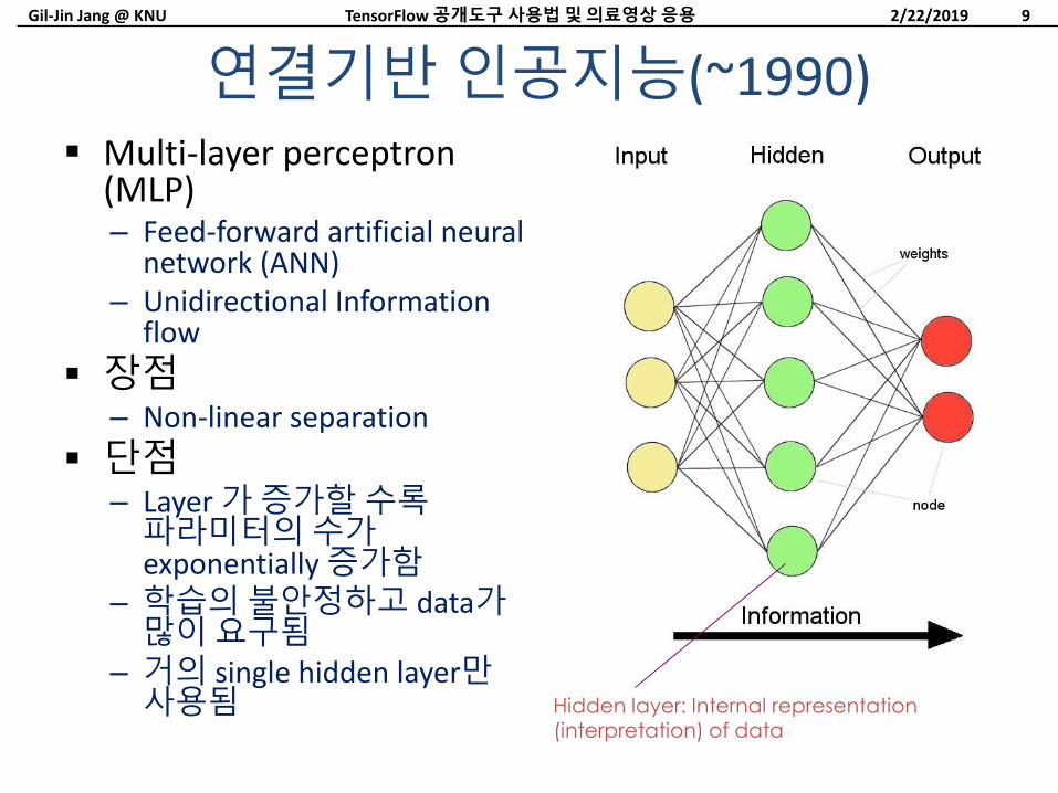
연결기반인공지능(~1990) Multi-layer perceptron
(MLP)– Feed-forward artificial neural
network (ANN)– Unidirectional Information
flow
장점– Non-linear separation
단점– Layer 가증가할수록파라미터의수가exponentially 증가함
– 학습의불안정하고 data가많이요구됨
– 거의 single hidden layer만사용됨
2/22/2019TensorFlow 공개도구사용법및의료영상응용 9
Hidden layer: Internal representation (interpretation) of data
Gil-Jin Jang @ KNU
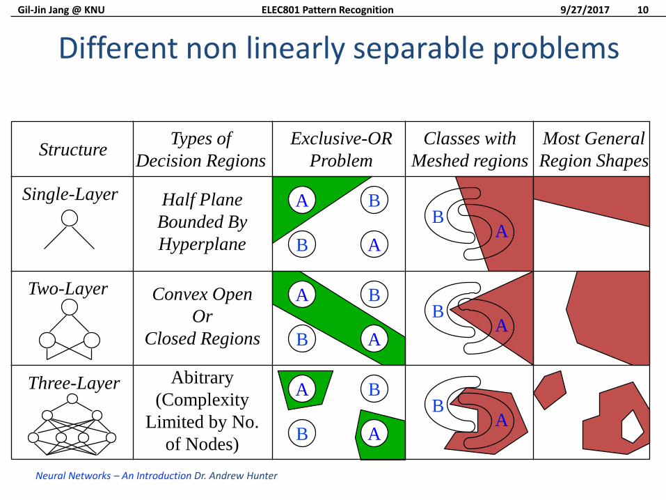
StructureTypes of
Decision Regions
Exclusive-OR
Problem
Classes with
Meshed regions
Most General
Region Shapes
Single-Layer
Two-Layer
Three-Layer
Half Plane
Bounded By
Hyperplane
Convex Open
Or
Closed Regions
Abitrary
(Complexity
Limited by No.
of Nodes)
A
AB
B
A
AB
B
A
AB
B
BA
BA
BA
Different non linearly separable problems
9/27/2017ELEC801 Pattern Recognition 10
Neural Networks – An Introduction Dr. Andrew Hunter
Gil-Jin Jang @ KNU
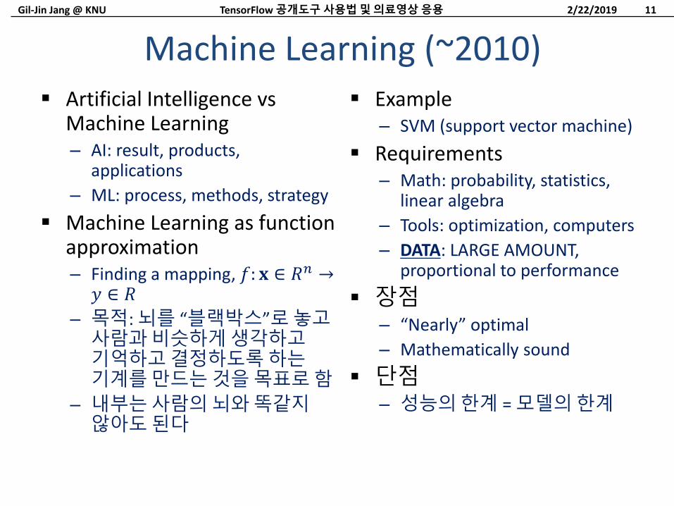
Machine Learning (~2010) Artificial Intelligence vs
Machine Learning– AI: result, products,
applications
– ML: process, methods, strategy
Machine Learning as function approximation– Finding a mapping, 𝑓: 𝐱 ∈ 𝑅𝑛 →𝑦 ∈ 𝑅
– 목적: 뇌를 “블랙박스”로놓고사람과비슷하게생각하고기억하고결정하도록하는기계를만드는것을목표로함
– 내부는사람의뇌와똑같지않아도된다
Example– SVM (support vector machine)
Requirements– Math: probability, statistics,
linear algebra
– Tools: optimization, computers
– DATA: LARGE AMOUNT, proportional to performance
장점– “Nearly” optimal
– Mathematically sound
단점– 성능의한계 = 모델의한계
2/22/2019TensorFlow 공개도구사용법및의료영상응용 11
Gil-Jin Jang @ KNU
기존의 MLP의학습을획기적으로개선하여 hidden layer의수와구조를복잡하게하는것을가능하게함
– Computation: GPU – 단순한병렬연산을효율적으로
– Stability: ReLU activation – vanishing gradient 문제를해결하여학습의안정성을높임
– Open source: 코드를공개하여다양한개발자들의자연스럽게협력하여자연스럽게발전시키는생태계를만듦(Hinton, Bengio, etc.)
Success stories
– 다양한응용분야에서극적으로성공적인(dramatically successful) 결과를보임: ImageNet, AlphaGo, etc.
심화학습: Deep Learning (2010~)
2/22/2019TensorFlow 공개도구사용법및의료영상응용 13
Gil-Jin Jang @ KNU
DEEP LEARNING TASK:VISUAL OBJECT RECOGNITIONCNN Success Story in ILSVRC-2012 and Onward
2/22/2019TensorFlow 공개도구사용법및의료영상응용 14
Gil-Jin Jang @ KNU
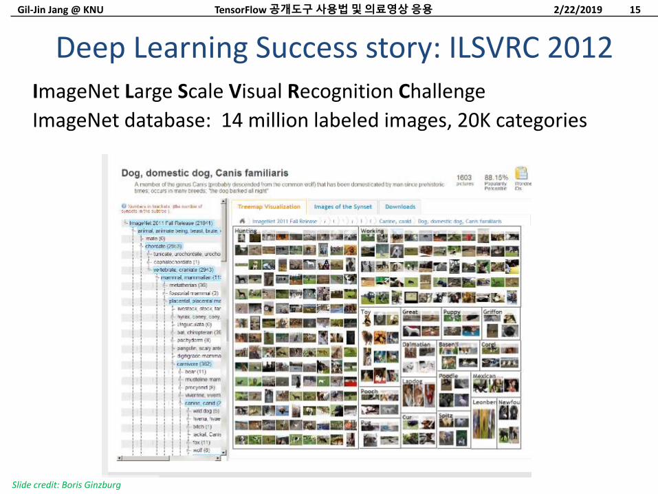
Deep Learning Success story: ILSVRC 2012ImageNet Large Scale Visual Recognition Challenge
ImageNet database: 14 million labeled images, 20K categories
2/22/2019TensorFlow 공개도구사용법및의료영상응용 15
Slide credit: Boris Ginzburg
Gil-Jin Jang @ KNU
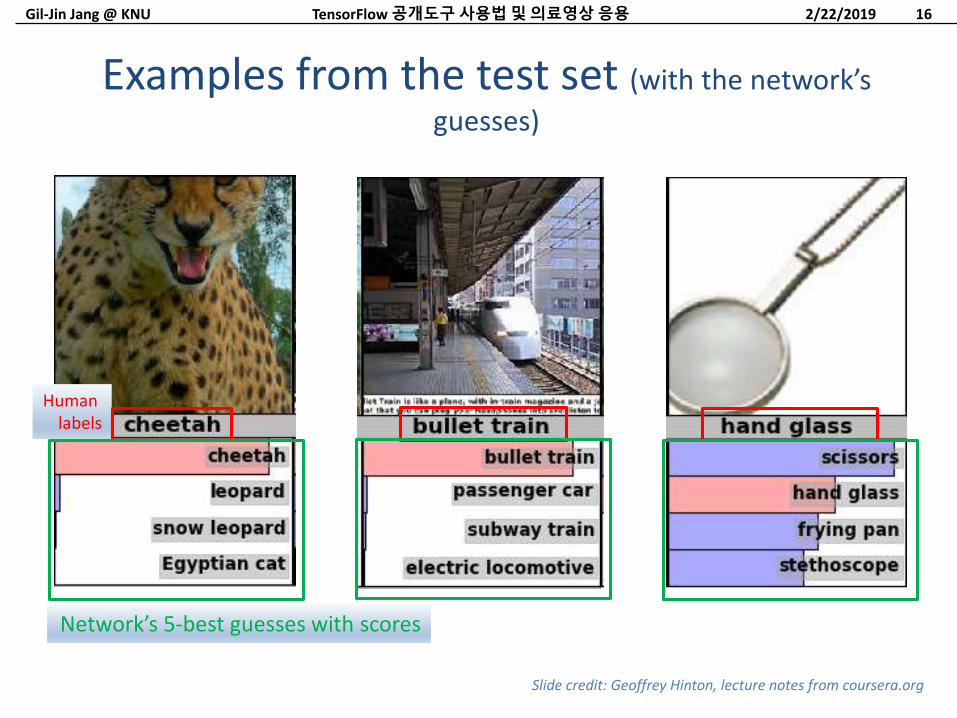
Examples from the test set (with the network’s
guesses)
2/22/2019TensorFlow 공개도구사용법및의료영상응용 16
Slide credit: Geoffrey Hinton, lecture notes from coursera.org
Human labels
Network’s 5-best guesses with scores
Gil-Jin Jang @ KNU
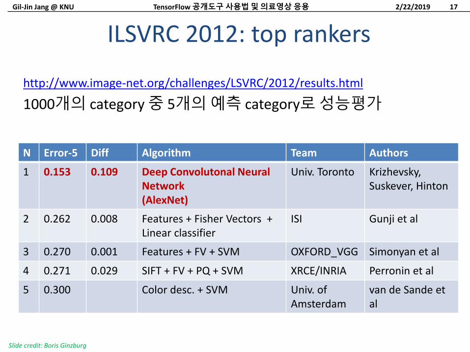
ILSVRC 2012: top rankers
http://www.image-net.org/challenges/LSVRC/2012/results.html
1000개의 category 중 5개의예측 category로성능평가
N Error-5 Diff Algorithm Team Authors
1 0.153 0.109 Deep Convolutonal Neural Network (AlexNet)
Univ. Toronto Krizhevsky, Suskever, Hinton
2 0.262 0.008 Features + Fisher Vectors + Linear classifier
ISI Gunji et al
3 0.270 0.001 Features + FV + SVM OXFORD_VGG Simonyan et al
4 0.271 0.029 SIFT + FV + PQ + SVM XRCE/INRIA Perronin et al
5 0.300 Color desc. + SVM Univ. of Amsterdam
van de Sande et al
2/22/2019TensorFlow 공개도구사용법및의료영상응용 17
Slide credit: Boris Ginzburg
Gil-Jin Jang @ KNU
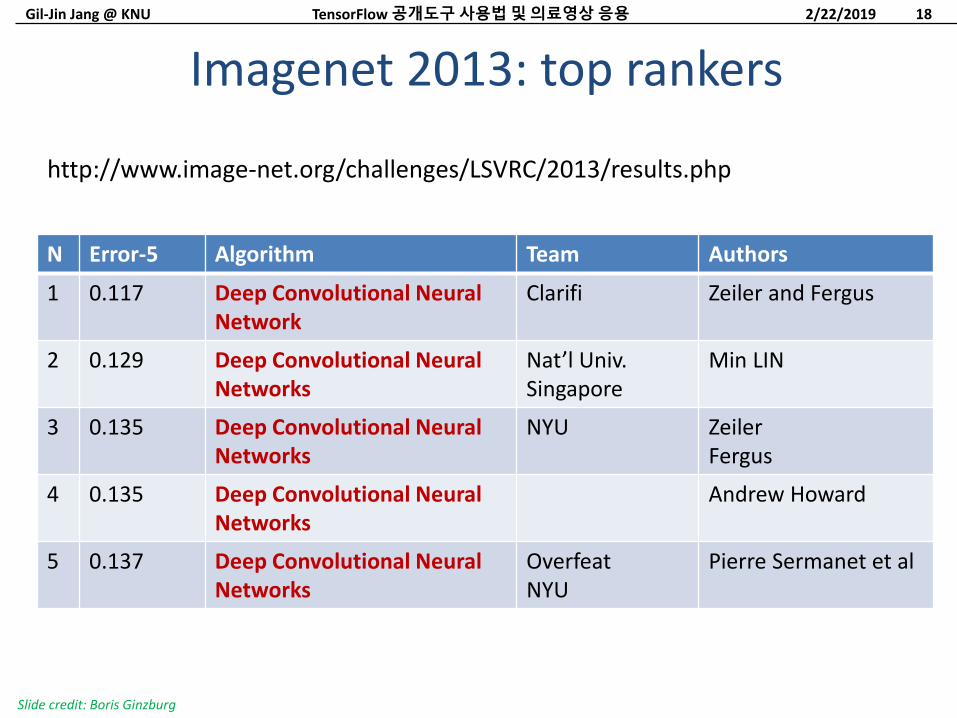
Imagenet 2013: top rankers
http://www.image-net.org/challenges/LSVRC/2013/results.php
N Error-5 Algorithm Team Authors
1 0.117 Deep Convolutional Neural Network
Clarifi Zeiler and Fergus
2 0.129 Deep Convolutional Neural Networks
Nat’l Univ.Singapore
Min LIN
3 0.135 Deep Convolutional Neural Networks
NYU ZeilerFergus
4 0.135 Deep Convolutional Neural Networks
Andrew Howard
5 0.137 Deep Convolutional Neural Networks
OverfeatNYU
Pierre Sermanet et al
2/22/2019TensorFlow 공개도구사용법및의료영상응용 18
Slide credit: Boris Ginzburg
Gil-Jin Jang @ KNU
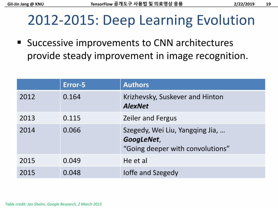
Successive improvements to CNN architectures provide steady improvement in image recognition.
2012-2015: Deep Learning Evolution
2/22/2019TensorFlow 공개도구사용법및의료영상응용 19
Error-5 Authors
2012 0.164 Krizhevsky, Suskever and HintonAlexNet
2013 0.115 Zeiler and Fergus
2014 0.066 Szegedy, Wei Liu, Yangqing Jia, …GoogLeNet,“Going deeper with convolutions”
2015 0.049 He et al
2015 0.048 Ioffe and Szegedy
Table credit: Jon Shelns, Google Research, 2 March 2015
Gil-Jin Jang @ KNU
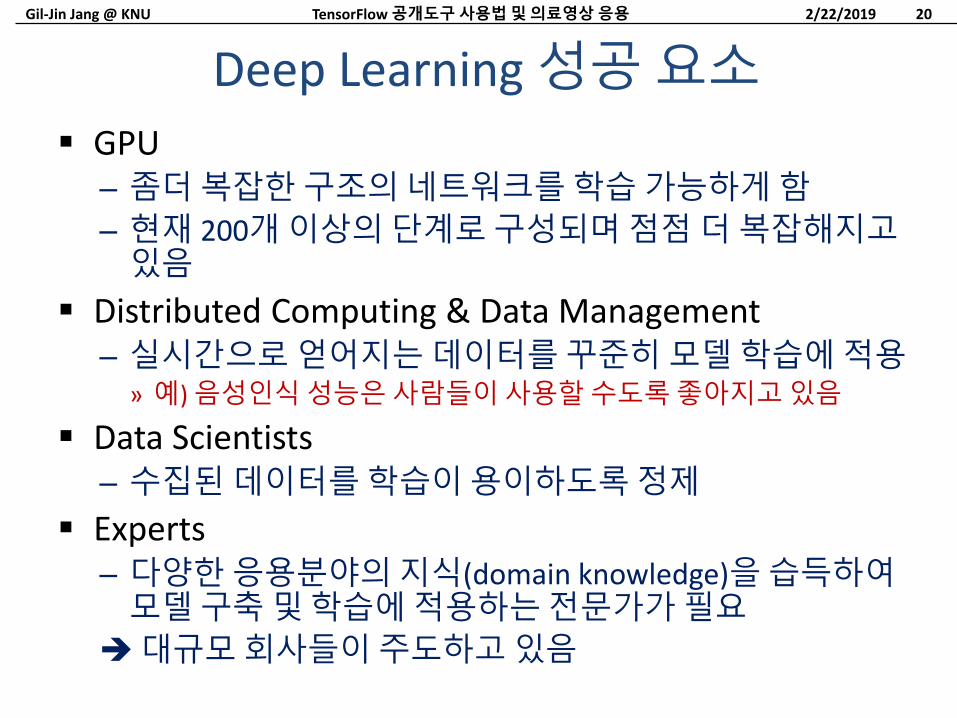
GPU– 좀더복잡한구조의네트워크를학습가능하게함
– 현재 200개이상의단계로구성되며점점더복잡해지고있음
Distributed Computing & Data Management– 실시간으로얻어지는데이터를꾸준히모델학습에적용
» 예) 음성인식성능은사람들이사용할수도록좋아지고있음
Data Scientists– 수집된데이터를학습이용이하도록정제
Experts– 다양한응용분야의지식(domain knowledge)을습득하여모델구축및학습에적용하는전문가가필요
대규모회사들이주도하고있음
Deep Learning 성공요소
2/22/2019TensorFlow 공개도구사용법및의료영상응용 20
Gil-Jin Jang @ KNU
CONVOLUTIONAL NEURAL NETWORKSOverview of the basic architecture
MNIST / CIFAR10 examples
Acknowledgments: Yann LeCun, Antonio Torralba, Boris Ginzburg
2/22/2019TensorFlow 공개도구사용법및의료영상응용 21
Gil-Jin Jang @ KNU
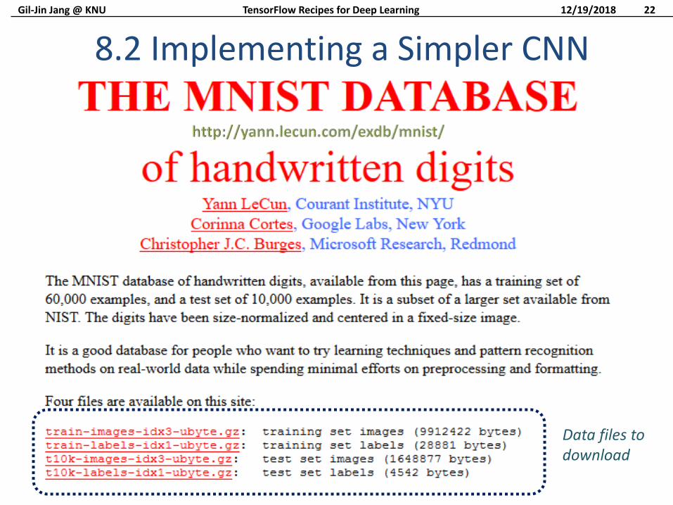
8.2 Implementing a Simpler CNN
12/19/2018TensorFlow Recipes for Deep Learning 22
Data files to download
Gil-Jin Jang @ KNU
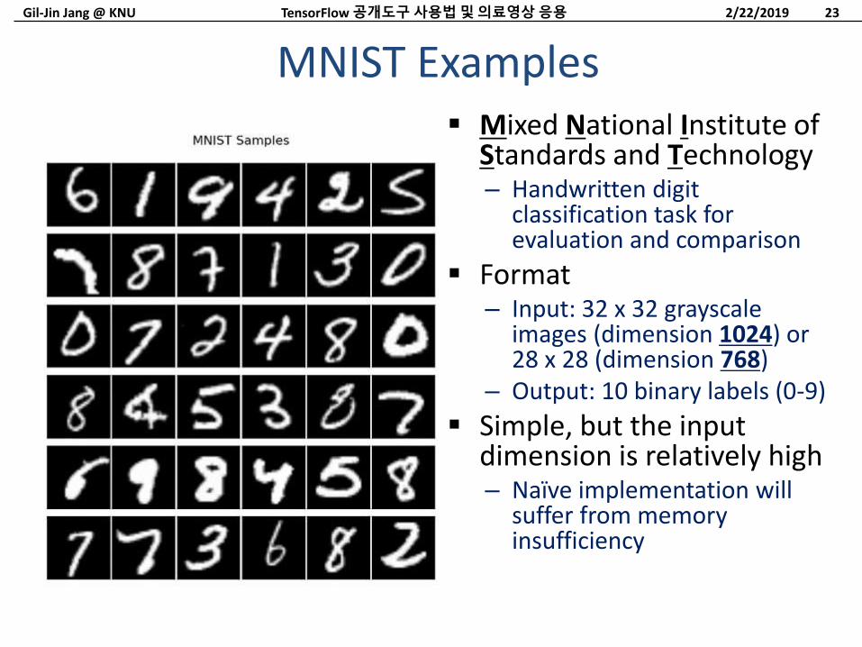
MNIST Examples Mixed National Institute of
Standards and Technology– Handwritten digit
classification task for evaluation and comparison
Format– Input: 32 x 32 grayscale
images (dimension 1024) or 28 x 28 (dimension 768)
– Output: 10 binary labels (0-9)
Simple, but the input dimension is relatively high– Naïve implementation will
suffer from memory insufficiency
2/22/2019TensorFlow 공개도구사용법및의료영상응용 23
Gil-Jin Jang @ KNU
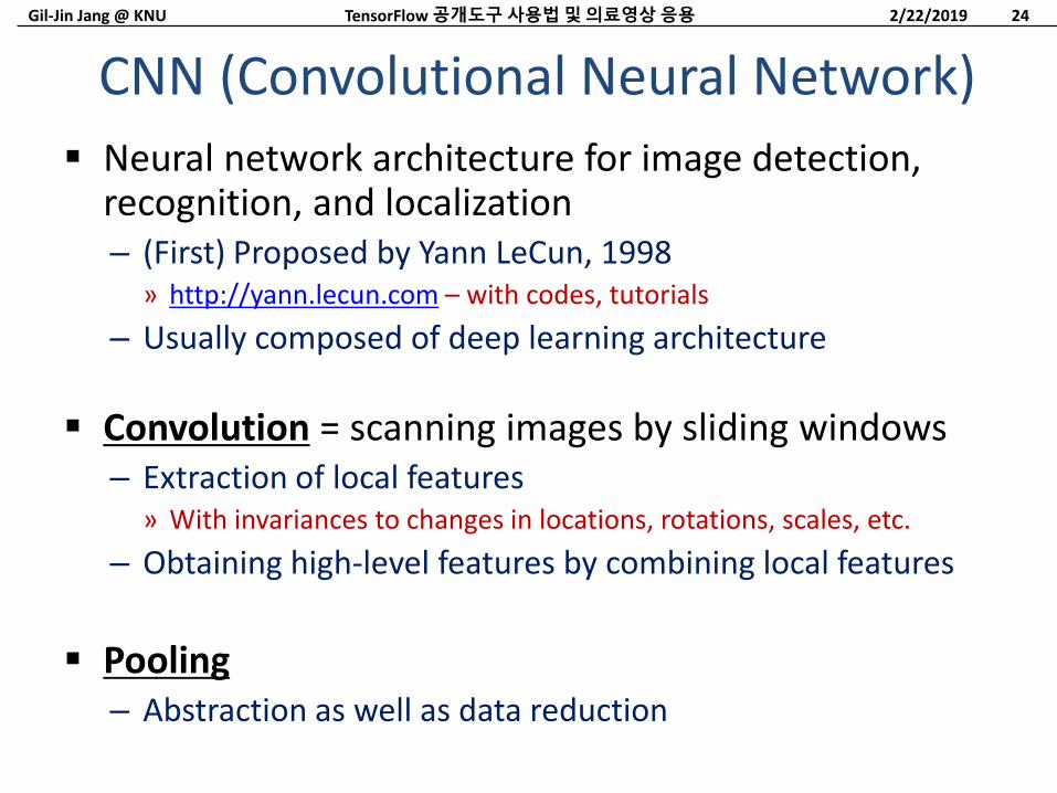
Neural network architecture for image detection, recognition, and localization– (First) Proposed by Yann LeCun, 1998
» http://yann.lecun.com – with codes, tutorials
– Usually composed of deep learning architecture
Convolution = scanning images by sliding windows– Extraction of local features
» With invariances to changes in locations, rotations, scales, etc.
– Obtaining high-level features by combining local features
Pooling– Abstraction as well as data reduction
CNN (Convolutional Neural Network)
2/22/2019TensorFlow 공개도구사용법및의료영상응용 24
Gil-Jin Jang @ KNU
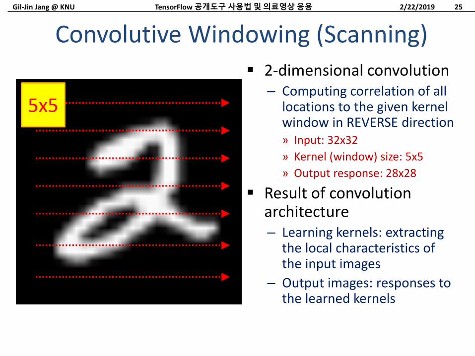
Convolutive Windowing (Scanning)
2-dimensional convolution– Computing correlation of all
locations to the given kernel window in REVERSE direction» Input: 32x32
» Kernel (window) size: 5x5
» Output response: 28x28
Result of convolution architecture– Learning kernels: extracting
the local characteristics of the input images
– Output images: responses to the learned kernels
2/22/2019TensorFlow 공개도구사용법및의료영상응용 25
5x5
Gil-Jin Jang @ KNU
Pooling (subsampling)
2/22/2019TensorFlow 공개도구사용법및의료영상응용 26
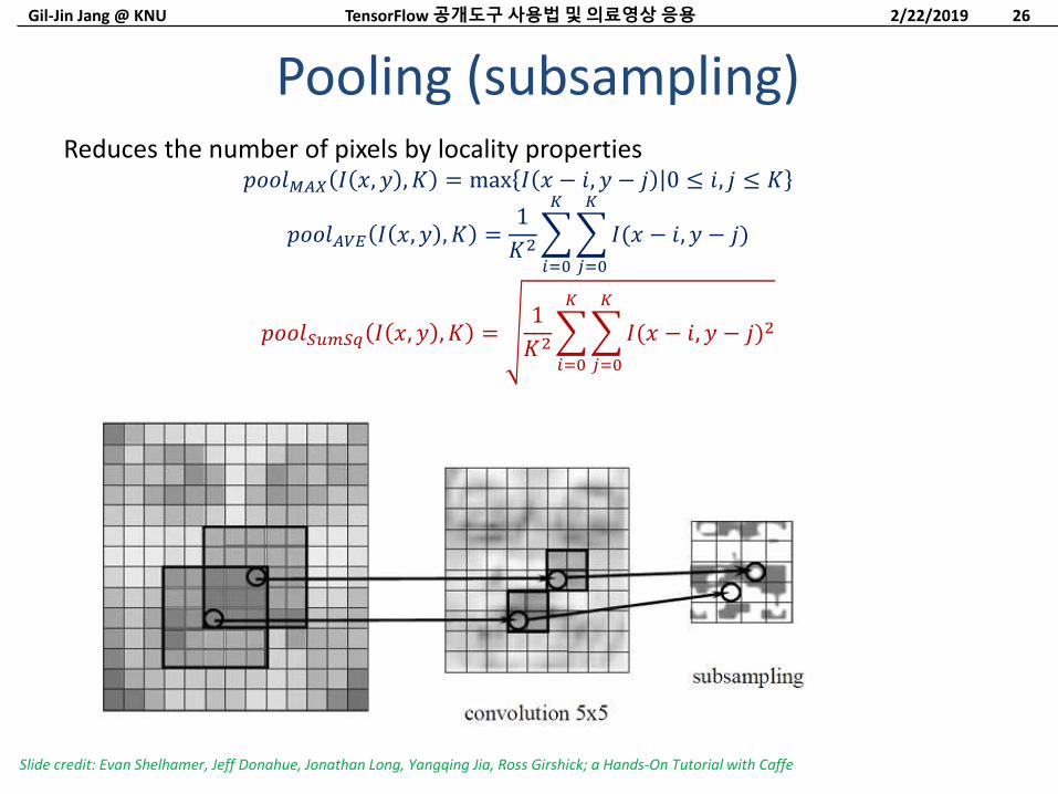
Reduces the number of pixels by locality properties𝑝𝑜𝑜𝑙𝑀𝐴𝑋 𝐼 𝑥, 𝑦 , 𝐾 = max 𝐼 𝑥 − 𝑖, 𝑦 − 𝑗 0 ≤ 𝑖, 𝑗 ≤ 𝐾
𝑝𝑜𝑜𝑙𝐴𝑉𝐸 𝐼 𝑥, 𝑦 , 𝐾 =1
𝐾2
𝑖=0
𝐾
𝑗=0
𝐾
𝐼(𝑥 − 𝑖, 𝑦 − 𝑗)
𝑝𝑜𝑜𝑙𝑆𝑢𝑚𝑆𝑞 𝐼 𝑥, 𝑦 , 𝐾 =1
𝐾2
𝑖=0
𝐾
𝑗=0
𝐾
𝐼(𝑥 − 𝑖, 𝑦 − 𝑗)2
Slide credit: Evan Shelhamer, Jeff Donahue, Jonathan Long, Yangqing Jia, Ross Girshick; a Hands-On Tutorial with Caffe
Gil-Jin Jang @ KNU
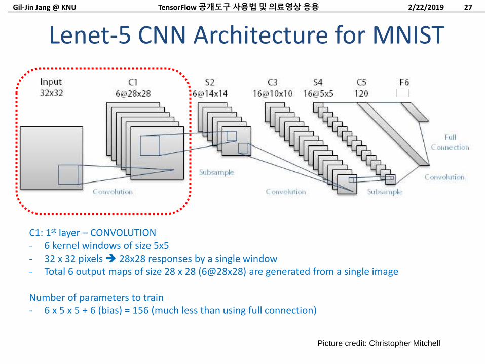
Lenet-5 CNN Architecture for MNIST
2/22/2019TensorFlow 공개도구사용법및의료영상응용 27
Picture credit: Christopher Mitchell
C1: 1st layer – CONVOLUTION- 6 kernel windows of size 5x5- 32 x 32 pixels 28x28 responses by a single window- Total 6 output maps of size 28 x 28 (6@28x28) are generated from a single image
Number of parameters to train- 6 x 5 x 5 + 6 (bias) = 156 (much less than using full connection)
Gil-Jin Jang @ KNU
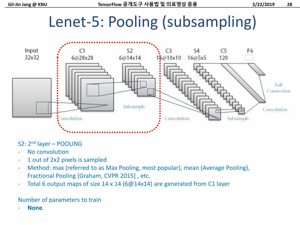
Lenet-5: Pooling (subsampling)
2/22/2019TensorFlow 공개도구사용법및의료영상응용 28
S2: 2nd layer – POOLING- No convolution- 1 out of 2x2 pixels is sampled- Method: max (referred to as Max Pooling, most popular), mean (Average Pooling),
Fractional Pooling [Graham, CVPR 2015] , etc.- Total 6 output maps of size 14 x 14 (6@14x14) are generated from C1 layer
Number of parameters to train- None.
Gil-Jin Jang @ KNU
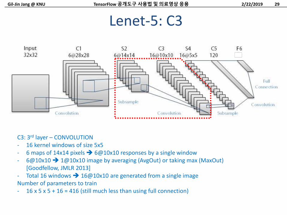
Lenet-5: C3
2/22/2019TensorFlow 공개도구사용법및의료영상응용 29
C3: 3rd layer – CONVOLUTION- 16 kernel windows of size 5x5- 6 maps of 14x14 pixels 6@10x10 responses by a single window- 6@10x10 1@10x10 image by averaging (AvgOut) or taking max (MaxOut)
[Goodfellow, JMLR 2013]- Total 16 windows 16@10x10 are generated from a single imageNumber of parameters to train- 16 x 5 x 5 + 16 = 416 (still much less than using full connection)
Gil-Jin Jang @ KNU
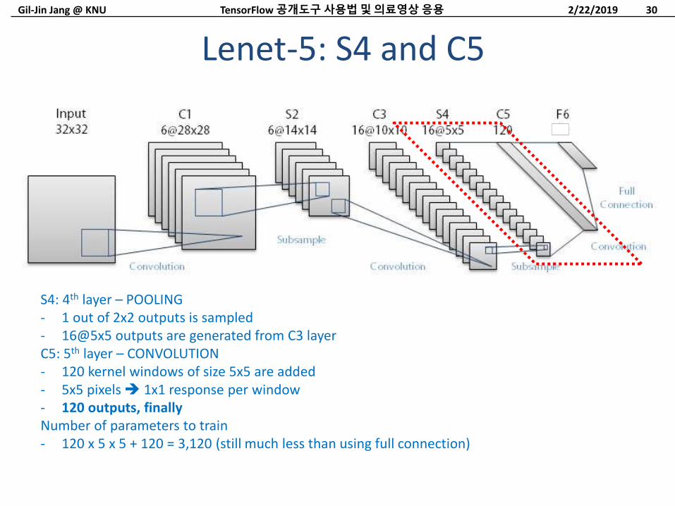
Lenet-5: S4 and C5
2/22/2019TensorFlow 공개도구사용법및의료영상응용 30
S4: 4th layer – POOLING- 1 out of 2x2 outputs is sampled- 16@5x5 outputs are generated from C3 layerC5: 5th layer – CONVOLUTION- 120 kernel windows of size 5x5 are added- 5x5 pixels 1x1 response per window- 120 outputs, finallyNumber of parameters to train- 120 x 5 x 5 + 120 = 3,120 (still much less than using full connection)
Gil-Jin Jang @ KNU
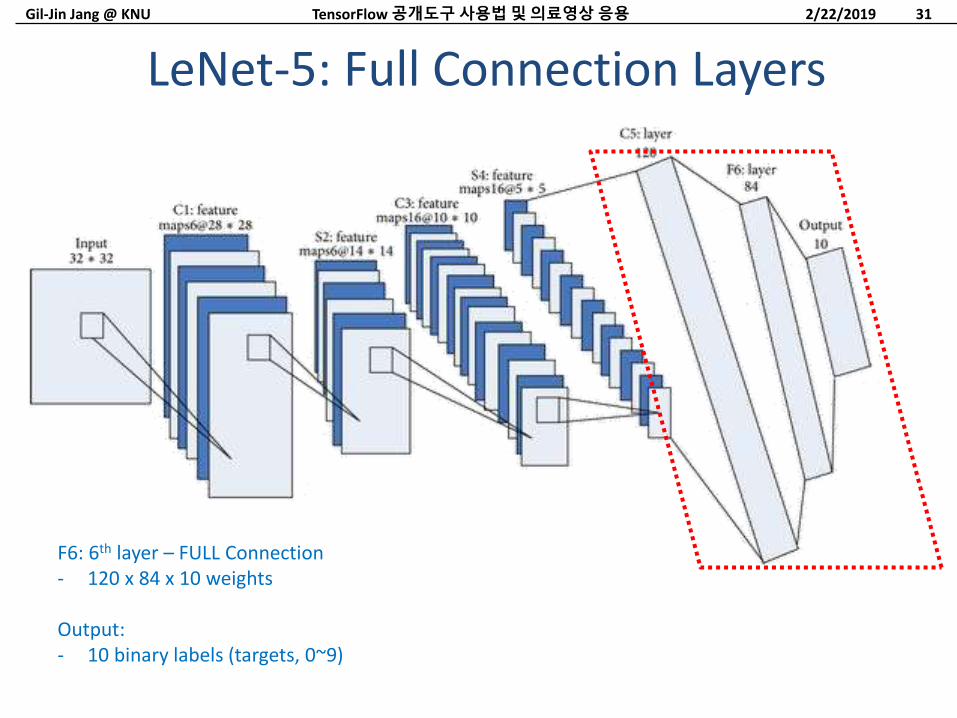
LeNet-5: Full Connection Layers
F6: 6th layer – FULL Connection- 120 x 84 x 10 weights
Output:- 10 binary labels (targets, 0~9)
2/22/2019TensorFlow 공개도구사용법및의료영상응용 31
Gil-Jin Jang @ KNU
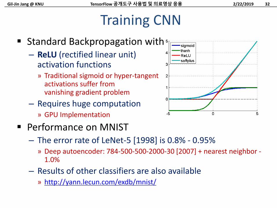
Standard Backpropagation with– ReLU (rectified linear unit)
activation functions» Traditional sigmoid or hyper-tangent
activations suffer fromvanishing gradient problem
– Requires huge computation» GPU Implementation
Performance on MNIST– The error rate of LeNet-5 [1998] is 0.8% - 0.95%
» Deep autoencoder: 784-500-500-2000-30 [2007] + nearest neighbor -1.0%
– Results of other classifiers are also available» http://yann.lecun.com/exdb/mnist/
Training CNN
2/22/2019TensorFlow 공개도구사용법및의료영상응용 32
Gil-Jin Jang @ KNU
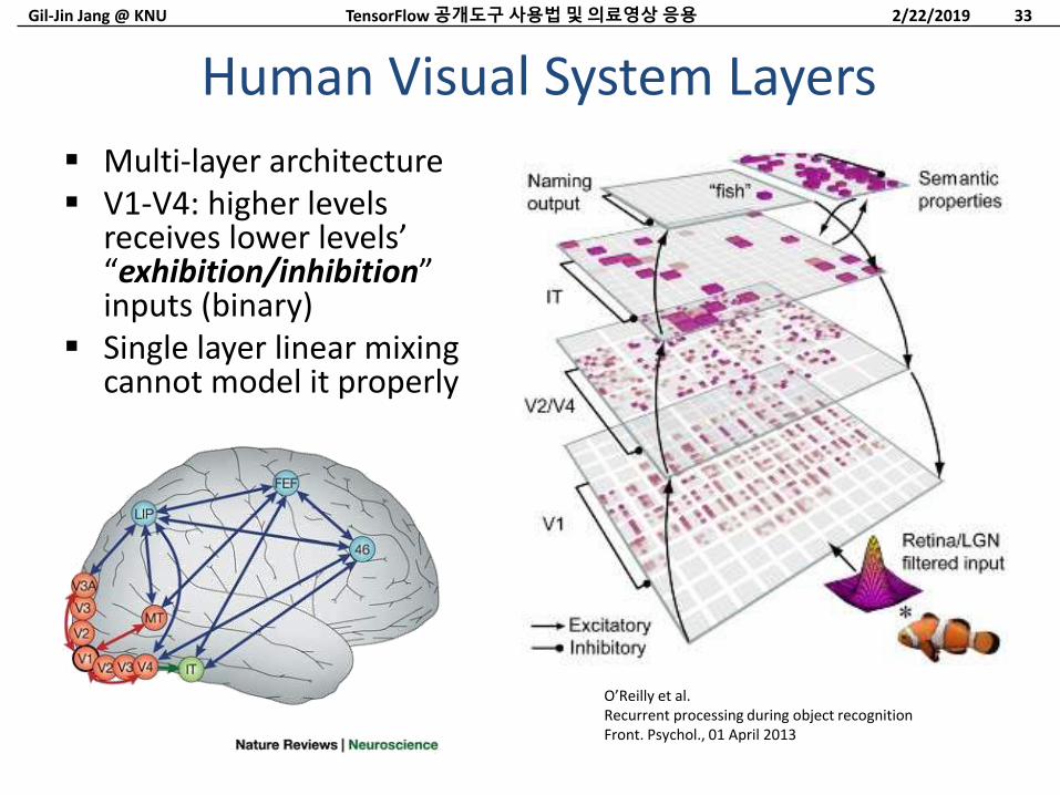
Multi-layer architecture V1-V4: higher levels
receives lower levels’ “exhibition/inhibition” inputs (binary)
Single layer linear mixing cannot model it properly
Human Visual System Layers
2/22/2019TensorFlow 공개도구사용법및의료영상응용 33
O’Reilly et al.Recurrent processing during object recognitionFront. Psychol., 01 April 2013
Gil-Jin Jang @ KNU
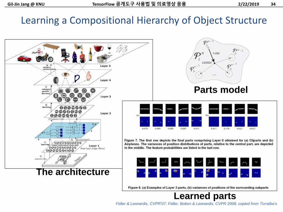
Learning a Compositional Hierarchy of Object Structure
The architecture
Parts model
Learned parts
2/22/2019TensorFlow 공개도구사용법및의료영상응용 34
Fidler & Leonardis, CVPR’07; Fidler, Boben & Leonardis, CVPR 2008, copied from Torralba’s
Gil-Jin Jang @ KNU
TENSORFLOW FOR DEEP LEARNING
2/22/2019TensorFlow 공개도구사용법및의료영상응용 35
Gil-Jin Jang @ KNU
TensorFlow Machine Learning Cookbook. Nick McClure. Packt Publishing. ISBN 978-1-78646-216-9.
Reason for the textbook choice
– Detailed explanation from the primitive features to the advanced problem solving
– TensorFlow is evolving so fast (like Android)» TensorFlow keeps being upgraded (r1.12 stable, as of December 12,
2018), but there exist huge number of older version codes (r0.x.x)
» Textbook is online, so the updates are being caught up
“Code is slowly becoming TensorFlow-v1.0.1 compliant.”
– Online recipes are available at:» http://www.packtpub.com/
» https://github.com/nfmcclure/tensorflow_cookbook
TextbookTensorFlow 공개도구사용법및의료영상응용 362/22/2019
Gil-Jin Jang @ KNU
Ch 1: Getting Started with TensorFlow
Ch 2: The TensorFlow Way
Ch 3: Linear Regression
Ch 4: Support Vector Machines
Ch 5: Nearest Neighbor Methods
Ch 6: Neural Networks
Ch 7: Natural Language Processing
Ch 8: Convolutional Neural Networks
Ch 9: Recurrent Neural Networks
Ch 10: Taking TensorFlow to Production
Ch 11: More with TensorFlow
Table of Contents
2/22/2019TensorFlow 공개도구사용법및의료영상응용 37
Gil-Jin Jang @ KNU
TensorFlow Installation
– See tensorflow.org
Python programming
– Including numpy
Deep learning theory
– DNN, CNN, RNN, SGD, etc.
Prerequisites
2/22/2019TensorFlow 공개도구사용법및의료영상응용 38
Gil-Jin Jang @ KNU
CHAPTER 1. GETTING STARTED WITHTENSORFLOW
2/22/2019TensorFlow 공개도구사용법및의료영상응용 39
Gil-Jin Jang @ KNU
1.1 How TensorFlow Works
1.2 Declaring Variables and Tensors
1.3 Using Placeholders and Variables
*1.4 Working with Matrices
1.5 Declaring Operations
1.6 Implementing Activation Functions – Chapter 2
*1.7 Working with Data Sources
Chapter 1 Contents
2/22/2019TensorFlow 공개도구사용법및의료영상응용 40
Gil-Jin Jang @ KNU
1.1 How TensorFlow Works
2/22/2019TensorFlow 공개도구사용법및의료영상응용 41
Gil-Jin Jang @ KNU
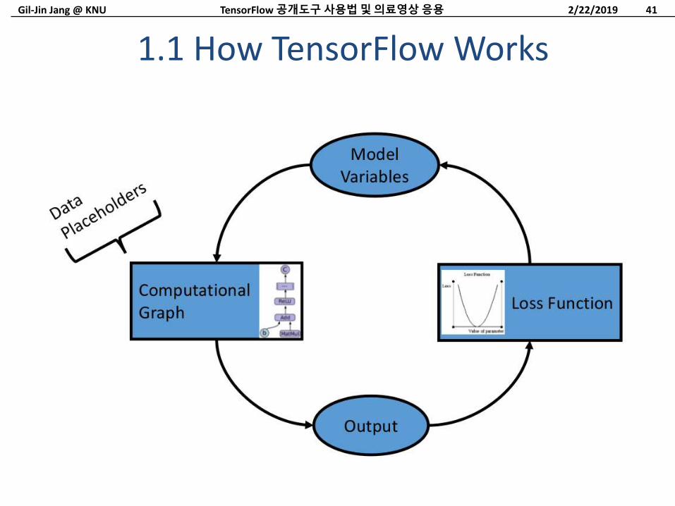
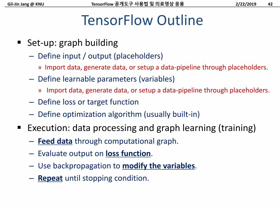
Set-up: graph building
– Define input / output (placeholders)
» Import data, generate data, or setup a data-pipeline through placeholders.
– Define learnable parameters (variables)
» Import data, generate data, or setup a data-pipeline through placeholders.
– Define loss or target function
– Define optimization algorithm (usually built-in)
Execution: data processing and graph learning (training)
– Feed data through computational graph.
– Evaluate output on loss function.
– Use backpropagation to modify the variables.
– Repeat until stopping condition.
TensorFlow Outline
2/22/2019TensorFlow 공개도구사용법및의료영상응용 42
Gil-Jin Jang @ KNU
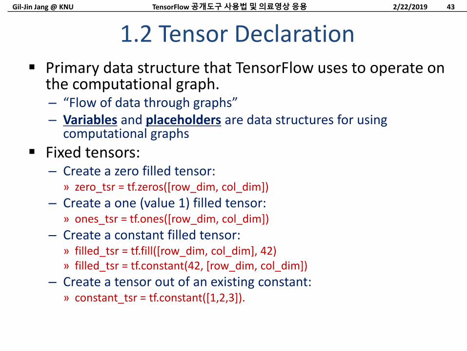
Primary data structure that TensorFlow uses to operate on the computational graph.– “Flow of data through graphs”– Variables and placeholders are data structures for using
computational graphs
Fixed tensors:– Create a zero filled tensor:
» zero_tsr = tf.zeros([row_dim, col_dim])
– Create a one (value 1) filled tensor:» ones_tsr = tf.ones([row_dim, col_dim])
– Create a constant filled tensor:» filled_tsr = tf.fill([row_dim, col_dim], 42)» filled_tsr = tf.constant(42, [row_dim, col_dim])
– Create a tensor out of an existing constant:» constant_tsr = tf.constant([1,2,3]).
1.2 Tensor Declaration
2/22/2019TensorFlow 공개도구사용법및의료영상응용 43
Gil-Jin Jang @ KNU
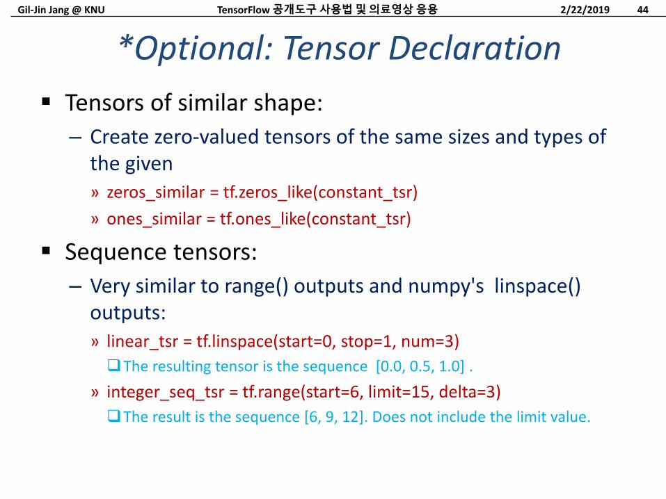
Tensors of similar shape:
– Create zero-valued tensors of the same sizes and types of the given» zeros_similar = tf.zeros_like(constant_tsr)
» ones_similar = tf.ones_like(constant_tsr)
Sequence tensors:
– Very similar to range() outputs and numpy's linspace() outputs:» linear_tsr = tf.linspace(start=0, stop=1, num=3)
The resulting tensor is the sequence [0.0, 0.5, 1.0] .
» integer_seq_tsr = tf.range(start=6, limit=15, delta=3)
The result is the sequence [6, 9, 12]. Does not include the limit value.
*Optional: Tensor Declaration
2/22/2019TensorFlow 공개도구사용법및의료영상응용 44
Gil-Jin Jang @ KNU
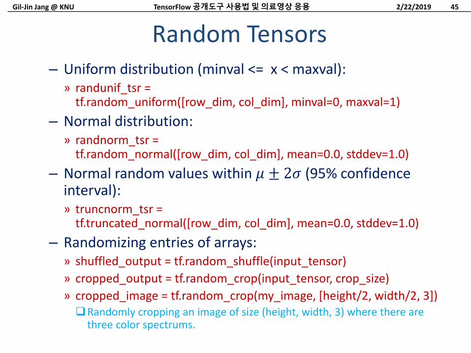
– Uniform distribution (minval <= x < maxval):» randunif_tsr =
tf.random_uniform([row_dim, col_dim], minval=0, maxval=1)
– Normal distribution:» randnorm_tsr =
tf.random_normal([row_dim, col_dim], mean=0.0, stddev=1.0)
– Normal random values within 𝜇 ± 2𝜎 (95% confidence interval):» truncnorm_tsr =
tf.truncated_normal([row_dim, col_dim], mean=0.0, stddev=1.0)
– Randomizing entries of arrays:» shuffled_output = tf.random_shuffle(input_tensor)
» cropped_output = tf.random_crop(input_tensor, crop_size)
» cropped_image = tf.random_crop(my_image, [height/2, width/2, 3])Randomly cropping an image of size (height, width, 3) where there are
three color spectrums.
Random Tensors
2/22/2019TensorFlow 공개도구사용법및의료영상응용 45
Gil-Jin Jang @ KNU
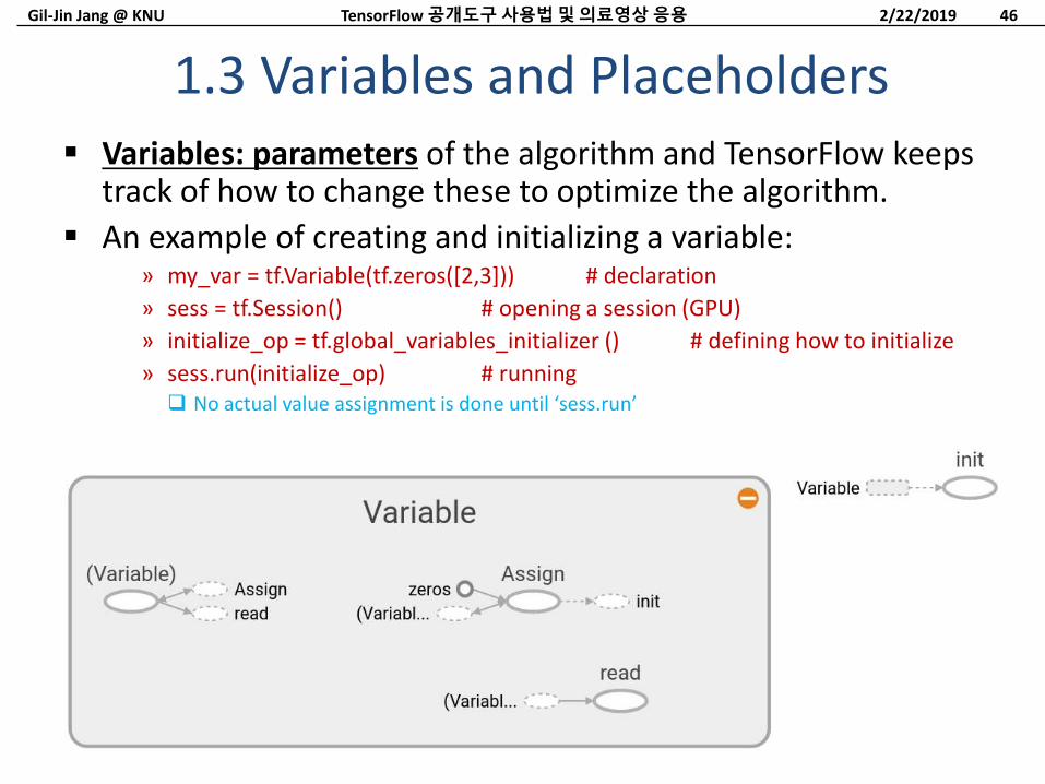
Variables: parameters of the algorithm and TensorFlow keeps track of how to change these to optimize the algorithm.
An example of creating and initializing a variable:» my_var = tf.Variable(tf.zeros([2,3])) # declaration
» sess = tf.Session() # opening a session (GPU)
» initialize_op = tf.global_variables_initializer () # defining how to initialize
» sess.run(initialize_op) # running No actual value assignment is done until ‘sess.run’
1.3 Variables and Placeholders
2/22/2019TensorFlow 공개도구사용법및의료영상응용 46
Gil-Jin Jang @ KNU
Variables from tensors:
– Usually learnable parameters, such as Neural Network weights.
– Create the corresponding variables by wrapping the tensor:» my_var = tf.Variable(tf.zeros([row_dim, col_dim]))
Variables from numpy arrays, or constant:
– convert_to_tensor(value, dtype=None, name=None, preferred_dtype=None)» convert_to_tensor (tf.constant([[1.0, 2.0], [3.0, 4.0]]))
» convert_to_tensor ([[1.0, 2.0], [3.0, 4.0]])
» convert_to_tensor(np.array([[1.0, 2.0], [3.0, 4.0]], dtype=np.float32))
*Optional: Conversion to Variables
2/22/2019TensorFlow 공개도구사용법및의료영상응용 47
Gil-Jin Jang @ KNU
Most common way is global_variables_initializer(), creating an operation in the graph that initializes all the variables we have created:
» initializer_op = tf.global_variables_initializer ()
But if we want to initialize a variable based on the results of initializing another variable:
» sess = tf.Session()
» first_var = tf.Variable(tf.zeros([2,3]))
» sess.run(first_var.initializer)
» second_var = tf.Variable(tf.zeros_like(first_var))
Depends on first_var
» sess.run(second_var.initializer)
Various Initialization Methods
2/22/2019TensorFlow 공개도구사용법및의료영상응용 48
Gil-Jin Jang @ KNU
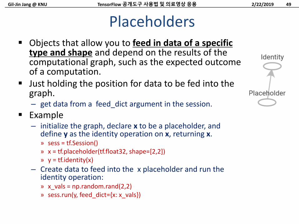
Objects that allow you to feed in data of a specific type and shape and depend on the results of the computational graph, such as the expected outcome of a computation.
Just holding the position for data to be fed into the graph.– get data from a feed_dict argument in the session.
Example– initialize the graph, declare x to be a placeholder, and
define y as the identity operation on x, returning x.» sess = tf.Session()» x = tf.placeholder(tf.float32, shape=[2,2])» y = tf.identity(x)
– Create data to feed into the x placeholder and run the identity operation:» x_vals = np.random.rand(2,2)» sess.run(y, feed_dict={x: x_vals})
Placeholders
2/22/2019TensorFlow 공개도구사용법및의료영상응용 49
Gil-Jin Jang @ KNU
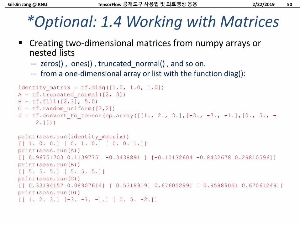
Creating two-dimensional matrices from numpy arrays or nested lists– zeros() , ones() , truncated_normal() , and so on. – from a one-dimensional array or list with the function diag():
*Optional: 1.4 Working with Matrices
2/22/2019TensorFlow 공개도구사용법및의료영상응용 50
identity_matrix = tf.diag([1.0, 1.0, 1.0])
A = tf.truncated_normal([2, 3])
B = tf.fill([2,3], 5.0)
C = tf.random_uniform([3,2])
D = tf.convert_to_tensor(np.array([[1., 2., 3.],[-3., -7., -1.],[0., 5., -
2.]]))
print(sess.run(identity_matrix))
[[ 1. 0. 0.] [ 0. 1. 0.] [ 0. 0. 1.]]
print(sess.run(A))
[[ 0.96751703 0.11397751 -0.3438891 ] [-0.10132604 -0.8432678 0.29810596]]
print(sess.run(B))
[[ 5. 5. 5.] [ 5. 5. 5.]]
print(sess.run(C))
[[ 0.33184157 0.08907614] [ 0.53189191 0.67605299] [ 0.95889051 0.67061249]]
print(sess.run(D))
[[ 1. 2. 3.] [-3. -7. -1.] [ 0. 5. -2.]]
Gil-Jin Jang @ KNU
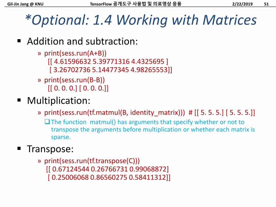
Addition and subtraction:» print(sess.run(A+B))
[[ 4.61596632 5.39771316 4.4325695 ][ 3.26702736 5.14477345 4.98265553]]
» print(sess.run(B-B))[[ 0. 0. 0.] [ 0. 0. 0.]]
Multiplication:» print(sess.run(tf.matmul(B, identity_matrix))) # [[ 5. 5. 5.] [ 5. 5. 5.]]The function matmul() has arguments that specify whether or not to
transpose the arguments before multiplication or whether each matrix is sparse.
Transpose:» print(sess.run(tf.transpose(C)))
[[ 0.67124544 0.26766731 0.99068872][ 0.25006068 0.86560275 0.58411312]]
*Optional: 1.4 Working with Matrices
2/22/2019TensorFlow 공개도구사용법및의료영상응용 51
Gil-Jin Jang @ KNU
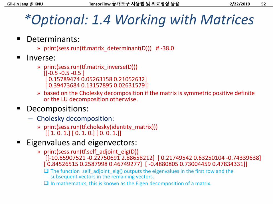
Determinants:» print(sess.run(tf.matrix_determinant(D))) # -38.0
Inverse:» print(sess.run(tf.matrix_inverse(D)))
[[-0.5 -0.5 -0.5 ][ 0.15789474 0.05263158 0.21052632][ 0.39473684 0.13157895 0.02631579]]
» based on the Cholesky decomposition if the matrix is symmetric positive definite or the LU decomposition otherwise.
Decompositions:– Cholesky decomposition:
» print(sess.run(tf.cholesky(identity_matrix)))[[ 1. 0. 1.] [ 0. 1. 0.] [ 0. 0. 1.]]
Eigenvalues and eigenvectors:» print(sess.run(tf.self_adjoint_eig(D))
[[-10.65907521 -0.22750691 2.88658212] [ 0.21749542 0.63250104 -0.74339638] [ 0.84526515 0.2587998 0.46749277] [ -0.4880805 0.73004459 0.47834331]] The function self_adjoint_eig() outputs the eigenvalues in the first row and the
subsequent vectors in the remaining vectors. In mathematics, this is known as the Eigen decomposition of a matrix.
*Optional: 1.4 Working with Matrices
2/22/2019TensorFlow 공개도구사용법및의료영상응용 52
Gil-Jin Jang @ KNU
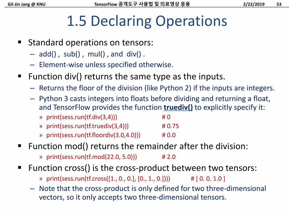
Standard operations on tensors:– add() , sub() , mul() , and div() .
– Element-wise unless specified otherwise.
Function div() returns the same type as the inputs.– Returns the floor of the division (like Python 2) if the inputs are integers.
– Python 3 casts integers into floats before dividing and returning a float, and TensorFlow provides the function truediv() to explicitly specify it:» print(sess.run(tf.div(3,4))) # 0
» print(sess.run(tf.truediv(3,4))) # 0.75
» print(sess.run(tf.floordiv(3.0,4.0))) # 0.0
Function mod() returns the remainder after the division:» print(sess.run(tf.mod(22.0, 5.0))) # 2.0
Function cross() is the cross-product between two tensors:» print(sess.run(tf.cross([1., 0., 0.], [0., 1., 0.]))) # [ 0. 0. 1.0 ]
– Note that the cross-product is only defined for two three-dimensional vectors, so it only accepts two three-dimensional tensors.
1.5 Declaring Operations
2/22/2019TensorFlow 공개도구사용법및의료영상응용 53
Gil-Jin Jang @ KNU
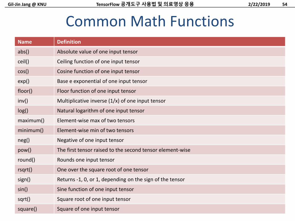
Name Definition
abs() Absolute value of one input tensor
ceil() Ceiling function of one input tensor
cos() Cosine function of one input tensor
exp() Base e exponential of one input tensor
floor() Floor function of one input tensor
inv() Multiplicative inverse (1/x) of one input tensor
log() Natural logarithm of one input tensor
maximum() Element-wise max of two tensors
minimum() Element-wise min of two tensors
neg() Negative of one input tensor
pow() The first tensor raised to the second tensor element-wise
round() Rounds one input tensor
rsqrt() One over the square root of one tensor
sign() Returns -1, 0, or 1, depending on the sign of the tensor
sin() Sine function of one input tensor
sqrt() Square root of one input tensor
square() Square of one input tensor
Common Math Functions
2/22/2019TensorFlow 공개도구사용법및의료영상응용 54
Gil-Jin Jang @ KNU
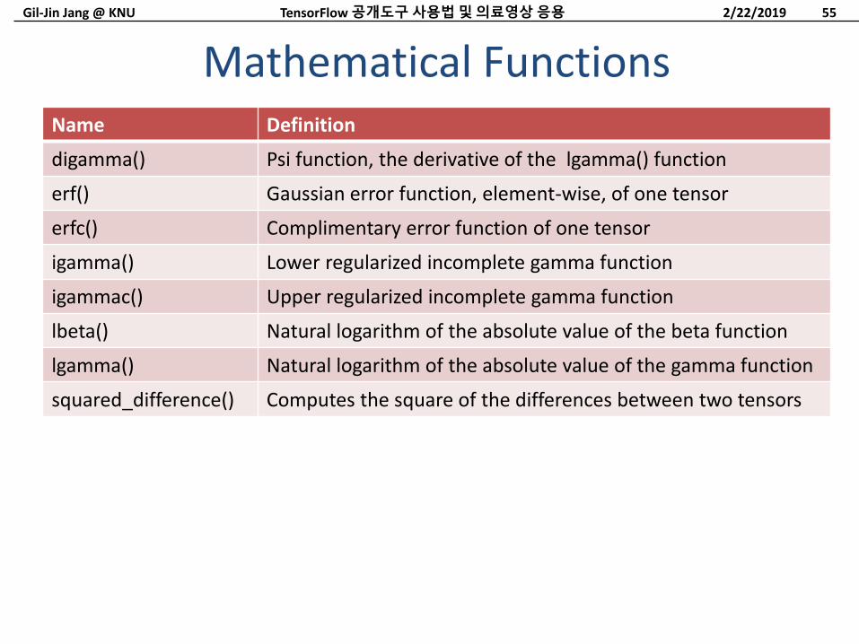
Name Definition
digamma() Psi function, the derivative of the lgamma() function
erf() Gaussian error function, element-wise, of one tensor
erfc() Complimentary error function of one tensor
igamma() Lower regularized incomplete gamma function
igammac() Upper regularized incomplete gamma function
lbeta() Natural logarithm of the absolute value of the beta function
lgamma() Natural logarithm of the absolute value of the gamma function
squared_difference() Computes the square of the differences between two tensors
Mathematical Functions
2/22/2019TensorFlow 공개도구사용법및의료영상응용 55
Gil-Jin Jang @ KNU
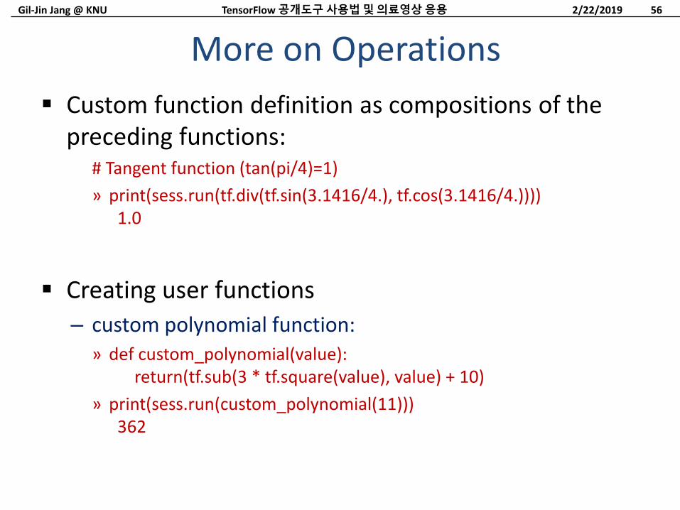
Custom function definition as compositions of the preceding functions:
# Tangent function (tan(pi/4)=1)
» print(sess.run(tf.div(tf.sin(3.1416/4.), tf.cos(3.1416/4.))))1.0
Creating user functions
– custom polynomial function:» def custom_polynomial(value):
return(tf.sub(3 * tf.square(value), value) + 10)
» print(sess.run(custom_polynomial(11)))362
More on Operations
2/22/2019TensorFlow 공개도구사용법및의료영상응용 56
Gil-Jin Jang @ KNU
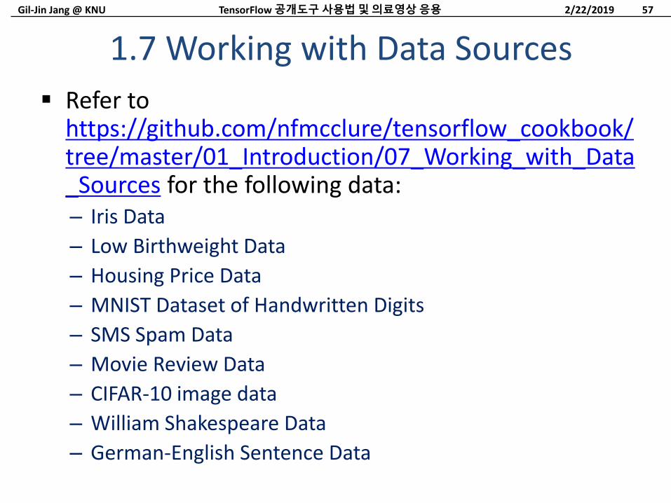
Refer to https://github.com/nfmcclure/tensorflow_cookbook/tree/master/01_Introduction/07_Working_with_Data_Sources for the following data:– Iris Data
– Low Birthweight Data
– Housing Price Data
– MNIST Dataset of Handwritten Digits
– SMS Spam Data
– Movie Review Data
– CIFAR-10 image data
– William Shakespeare Data
– German-English Sentence Data
1.7 Working with Data Sources
2/22/2019TensorFlow 공개도구사용법및의료영상응용 57
Gil-Jin Jang @ KNU
CHAPTER 2.THE TENSORFLOW WAY
2/22/2019TensorFlow 공개도구사용법및의료영상응용 58
Gil-Jin Jang @ KNU
2.1 Operations in a Computational Graph
2.2 Layering Nested Operations
2.3 Working with Multiple Layers
*1.6 Implementing Activation Functions
2.4 Implementing Loss Functions
2.5 Implementing Back Propagation
2.6 Working with Batch and Stochastic Training
2.7 Combining Everything Together
2.8 Evaluating Models
2. The TensorFlow Way
2/22/2019TensorFlow 공개도구사용법및의료영상응용 59
Gil-Jin Jang @ KNU
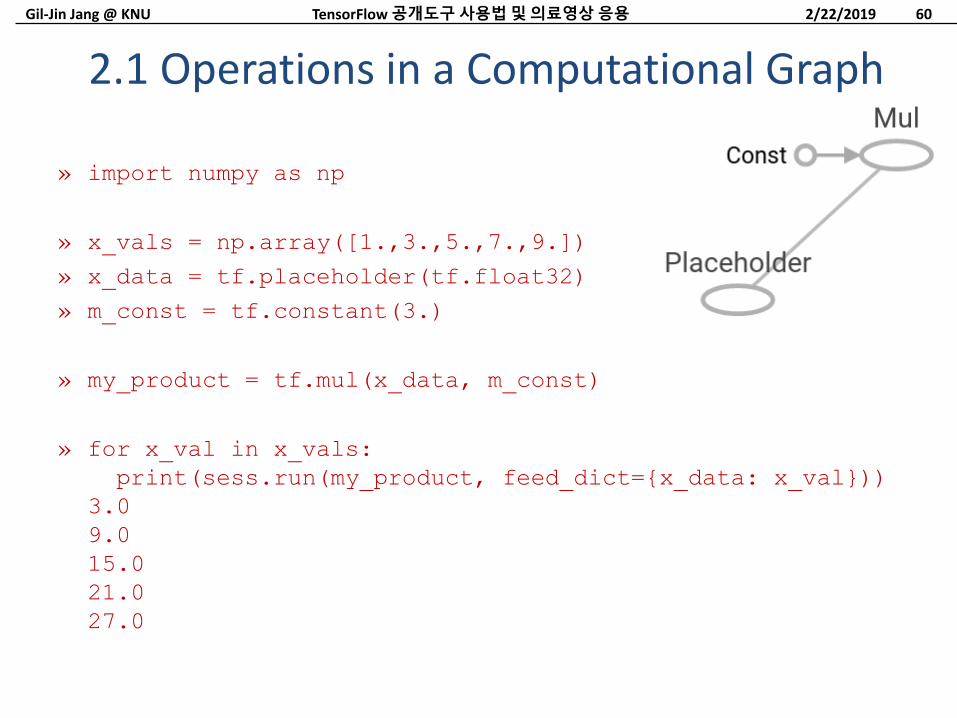
2.1 Operations in a Computational Graph
» import numpy as np
» x_vals = np.array([1.,3.,5.,7.,9.])
» x_data = tf.placeholder(tf.float32)
» m_const = tf.constant(3.)
» my_product = tf.mul(x_data, m_const)
» for x_val in x_vals:
print(sess.run(my_product, feed_dict={x_data: x_val}))
3.0
9.0
15.0
21.0
27.0
2/22/2019TensorFlow 공개도구사용법및의료영상응용 60
Gil-Jin Jang @ KNU
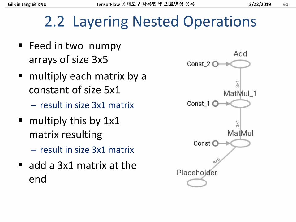
2.2 Layering Nested Operations
Feed in two numpyarrays of size 3x5
multiply each matrix by a constant of size 5x1
– result in size 3x1 matrix
multiply this by 1x1 matrix resulting
– result in size 3x1 matrix
add a 3x1 matrix at the end
2/22/2019TensorFlow 공개도구사용법및의료영상응용 61
Gil-Jin Jang @ KNU
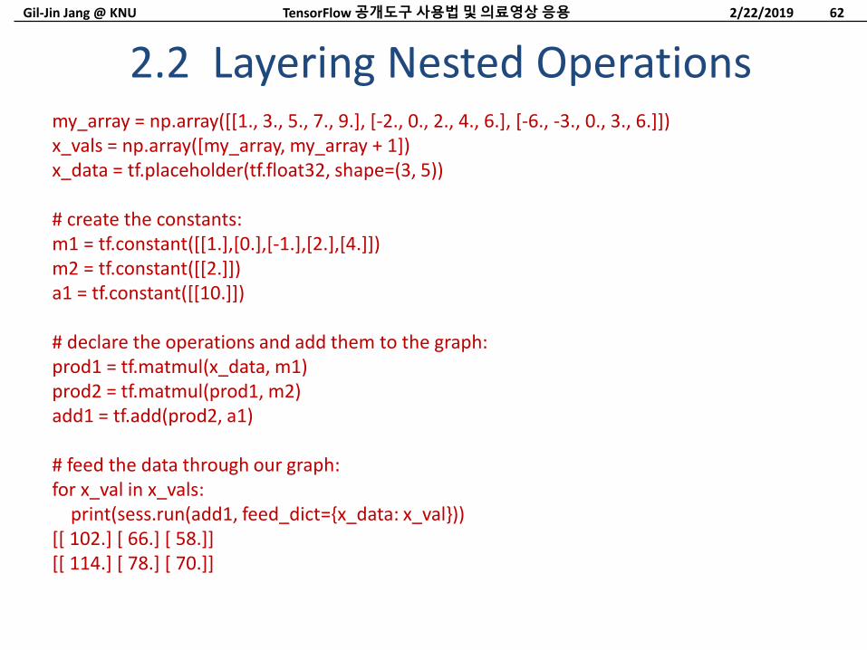
my_array = np.array([[1., 3., 5., 7., 9.], [-2., 0., 2., 4., 6.], [-6., -3., 0., 3., 6.]])x_vals = np.array([my_array, my_array + 1])x_data = tf.placeholder(tf.float32, shape=(3, 5))
# create the constants:m1 = tf.constant([[1.],[0.],[-1.],[2.],[4.]])m2 = tf.constant([[2.]])a1 = tf.constant([[10.]])
# declare the operations and add them to the graph:prod1 = tf.matmul(x_data, m1)prod2 = tf.matmul(prod1, m2)add1 = tf.add(prod2, a1)
# feed the data through our graph:for x_val in x_vals:
print(sess.run(add1, feed_dict={x_data: x_val}))[[ 102.] [ 66.] [ 58.]][[ 114.] [ 78.] [ 70.]]
2.2 Layering Nested Operations
2/22/2019TensorFlow 공개도구사용법및의료영상응용 62
Gil-Jin Jang @ KNU
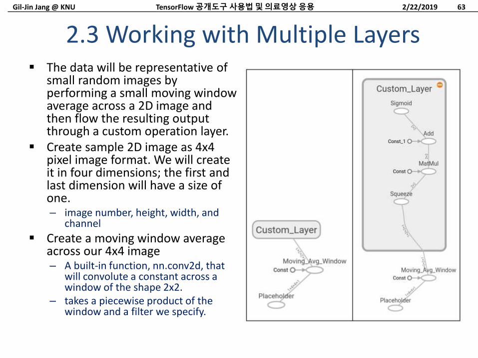
2.3 Working with Multiple Layers The data will be representative of
small random images by performing a small moving window average across a 2D image and then flow the resulting output through a custom operation layer.
Create sample 2D image as 4x4 pixel image format. We will create it in four dimensions; the first and last dimension will have a size of one.– image number, height, width, and
channel
Create a moving window average across our 4x4 image– A built-in function, nn.conv2d, that
will convolute a constant across a window of the shape 2x2.
– takes a piecewise product of the window and a filter we specify.
2/22/2019TensorFlow 공개도구사용법및의료영상응용 63
Gil-Jin Jang @ KNU
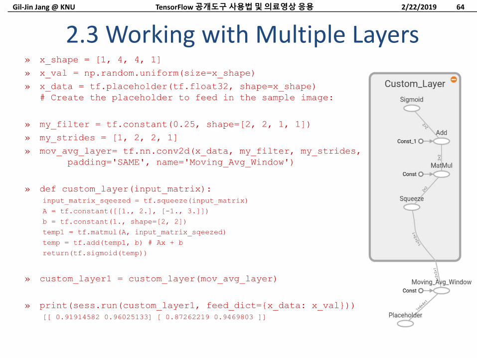
» x_shape = [1, 4, 4, 1]
» x_val = np.random.uniform(size=x_shape)
» x_data = tf.placeholder(tf.float32, shape=x_shape)
# Create the placeholder to feed in the sample image:
» my_filter = tf.constant(0.25, shape=[2, 2, 1, 1])
» my_strides = [1, 2, 2, 1]
» mov_avg_layer= tf.nn.conv2d(x_data, my_filter, my_strides,
padding='SAME', name='Moving_Avg_Window')
» def custom_layer(input_matrix):
input_matrix_sqeezed = tf.squeeze(input_matrix)
A = tf.constant([[1., 2.], [-1., 3.]])
b = tf.constant(1., shape=[2, 2])
temp1 = tf.matmul(A, input_matrix_sqeezed)
temp = tf.add(temp1, b) # Ax + b
return(tf.sigmoid(temp))
» custom_layer1 = custom_layer(mov_avg_layer)
» print(sess.run(custom_layer1, feed_dict={x_data: x_val}))
[[ 0.91914582 0.96025133] [ 0.87262219 0.9469803 ]]
2.3 Working with Multiple Layers
2/22/2019TensorFlow 공개도구사용법및의료영상응용 64
Gil-Jin Jang @ KNU
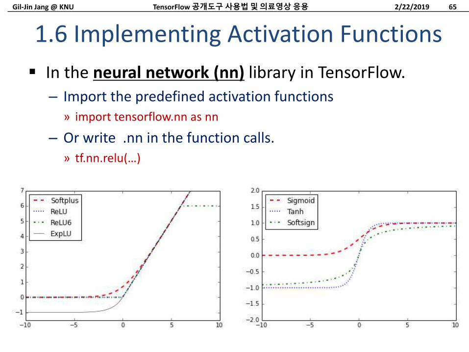
In the neural network (nn) library in TensorFlow.
– Import the predefined activation functions» import tensorflow.nn as nn
– Or write .nn in the function calls.» tf.nn.relu(…)
1.6 Implementing Activation Functions
2/22/2019TensorFlow 공개도구사용법및의료영상응용 65
Gil-Jin Jang @ KNU
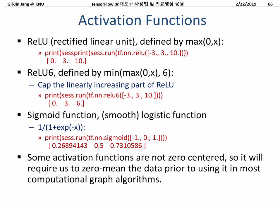
ReLU (rectified linear unit), defined by max(0,x):» print(sessprint(sess.run(tf.nn.relu([-3., 3., 10.])))
[ 0. 3. 10.]
ReLU6, defined by min(max(0,x), 6):– Cap the linearly increasing part of ReLU
» print(sess.run(tf.nn.relu6([-3., 3., 10.])))[ 0. 3. 6.]
Sigmoid function, (smooth) logistic function– 1/(1+exp(-x)):
» print(sess.run(tf.nn.sigmoid([-1., 0., 1.])))[ 0.26894143 0.5 0.7310586 ]
Some activation functions are not zero centered, so it will require us to zero-mean the data prior to using it in most computational graph algorithms.
Activation Functions
2/22/2019TensorFlow 공개도구사용법및의료영상응용 66
Gil-Jin Jang @ KNU
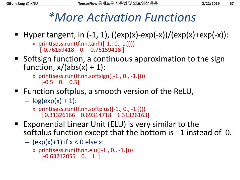
Hyper tangent, in (-1, 1), ((exp(x)-exp(-x))/(exp(x)+exp(-x)):» print(sess.run(tf.nn.tanh([-1., 0., 1.])))
[-0.76159418 0. 0.76159418 ]
Softsign function, a continuous approximation to the sign function, x/(abs(x) + 1):
» print(sess.run(tf.nn.softsign([-1., 0., -1.])))[-0.5 0. 0.5]
Function softplus, a smooth version of the ReLU, – log(exp(x) + 1):
» print(sess.run(tf.nn.softplus([-1., 0., -1.])))[ 0.31326166 0.69314718 1.31326163]
Exponential Linear Unit (ELU) is very similar to the softplus function except that the bottom is -1 instead of 0.– (exp(x)+1) if x < 0 else x:
» print(sess.run(tf.nn.elu([-1., 0., -1.])))[-0.63212055 0. 1. ]
*More Activation Functions
2/22/2019TensorFlow 공개도구사용법및의료영상응용 67
Gil-Jin Jang @ KNU
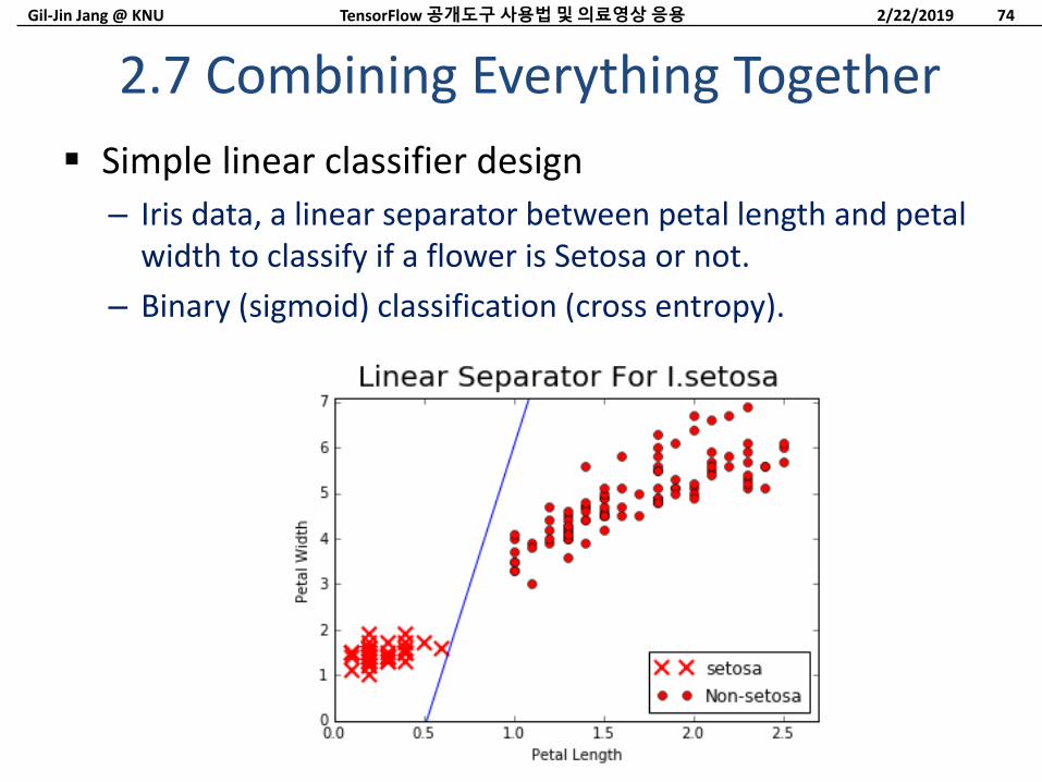
Simple linear classifier design
– Iris data, a linear separator between petal length and petal width to classify if a flower is Setosa or not.
– Binary (sigmoid) classification (cross entropy).
2.7 Combining Everything Together
2/22/2019TensorFlow 공개도구사용법및의료영상응용 74
Gil-Jin Jang @ KNU
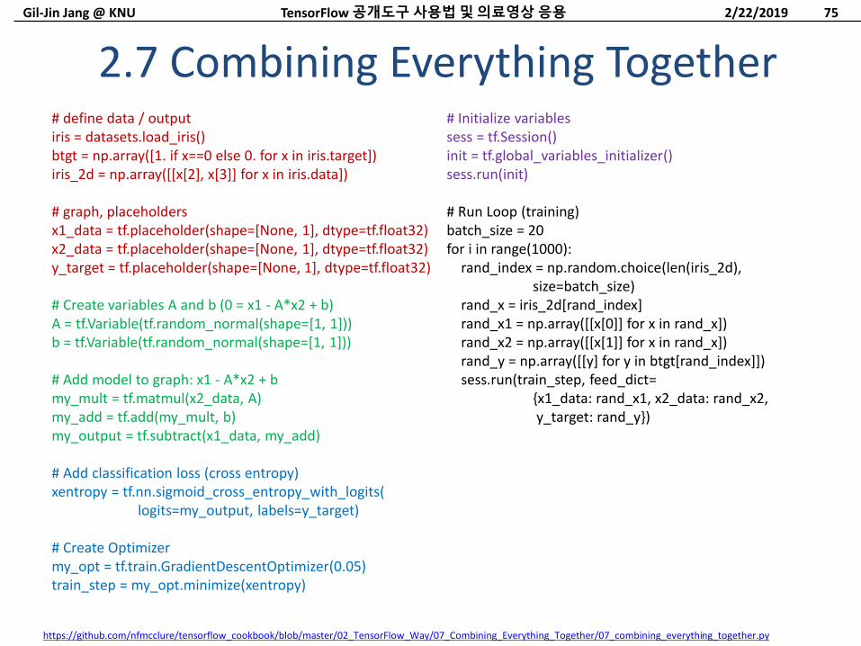
2.7 Combining Everything Together# define data / outputiris = datasets.load_iris()btgt = np.array([1. if x==0 else 0. for x in iris.target])iris_2d = np.array([[x[2], x[3]] for x in iris.data])
# graph, placeholdersx1_data = tf.placeholder(shape=[None, 1], dtype=tf.float32)x2_data = tf.placeholder(shape=[None, 1], dtype=tf.float32)y_target = tf.placeholder(shape=[None, 1], dtype=tf.float32)
# Create variables A and b (0 = x1 - A*x2 + b)A = tf.Variable(tf.random_normal(shape=[1, 1]))b = tf.Variable(tf.random_normal(shape=[1, 1]))
# Add model to graph: x1 - A*x2 + bmy_mult = tf.matmul(x2_data, A)my_add = tf.add(my_mult, b)my_output = tf.subtract(x1_data, my_add)
# Add classification loss (cross entropy)xentropy = tf.nn.sigmoid_cross_entropy_with_logits(
logits=my_output, labels=y_target)
# Create Optimizermy_opt = tf.train.GradientDescentOptimizer(0.05)train_step = my_opt.minimize(xentropy)
# Initialize variablessess = tf.Session()init = tf.global_variables_initializer()sess.run(init)
# Run Loop (training)batch_size = 20for i in range(1000):
rand_index = np.random.choice(len(iris_2d),size=batch_size)
rand_x = iris_2d[rand_index]rand_x1 = np.array([[x[0]] for x in rand_x])rand_x2 = np.array([[x[1]] for x in rand_x])rand_y = np.array([[y] for y in btgt[rand_index]])sess.run(train_step, feed_dict=
{x1_data: rand_x1, x2_data: rand_x2,y_target: rand_y})
2/22/2019TensorFlow 공개도구사용법및의료영상응용 75
https://github.com/nfmcclure/tensorflow_cookbook/blob/master/02_TensorFlow_Way/07_Combining_Everything_Together/07_combining_everything_together.py
Gil-Jin Jang @ KNU
CHAPTER 6.NEURAL NETWORKS
2/22/2019TensorFlow 공개도구사용법및의료영상응용 76
Gil-Jin Jang @ KNU
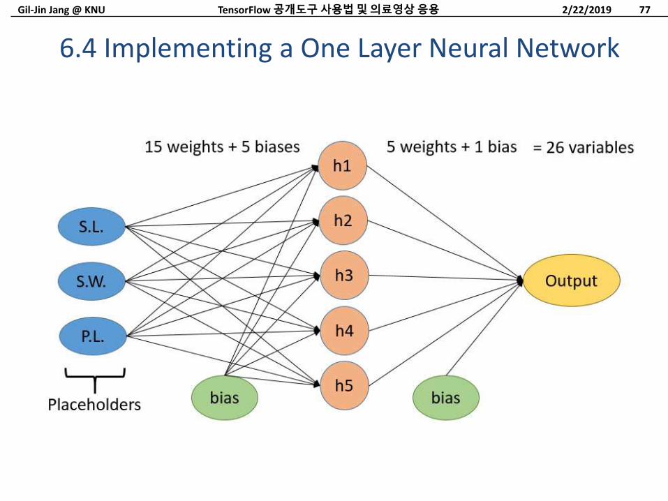
6.4 Implementing a One Layer Neural Network
2/22/2019TensorFlow 공개도구사용법및의료영상응용 77
Gil-Jin Jang @ KNU
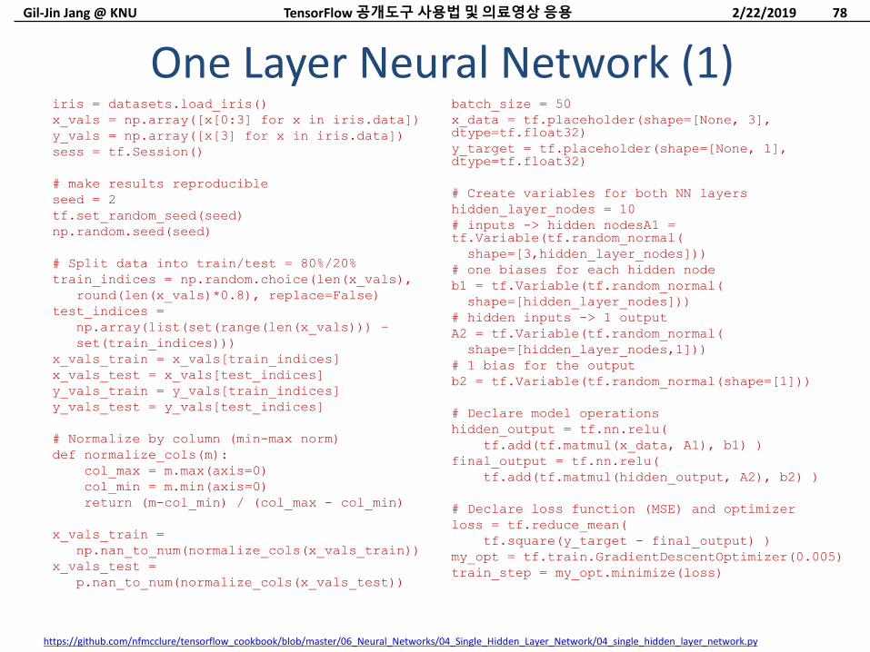
One Layer Neural Network (1)iris = datasets.load_iris()
x_vals = np.array([x[0:3] for x in iris.data])
y_vals = np.array([x[3] for x in iris.data])
sess = tf.Session()
# make results reproducible
seed = 2
tf.set_random_seed(seed)
np.random.seed(seed)
# Split data into train/test = 80%/20%
train_indices = np.random.choice(len(x_vals),
round(len(x_vals)*0.8), replace=False)
test_indices =
np.array(list(set(range(len(x_vals))) –
set(train_indices)))
x_vals_train = x_vals[train_indices]
x_vals_test = x_vals[test_indices]
y_vals_train = y_vals[train_indices]
y_vals_test = y_vals[test_indices]
# Normalize by column (min-max norm)
def normalize_cols(m):
col_max = m.max(axis=0)
col_min = m.min(axis=0)
return (m-col_min) / (col_max - col_min)
x_vals_train =
np.nan_to_num(normalize_cols(x_vals_train))
x_vals_test =
p.nan_to_num(normalize_cols(x_vals_test))
batch_size = 50
x_data = tf.placeholder(shape=[None, 3], dtype=tf.float32)
y_target = tf.placeholder(shape=[None, 1], dtype=tf.float32)
# Create variables for both NN layers
hidden_layer_nodes = 10
# inputs -> hidden nodesA1 = tf.Variable(tf.random_normal(
shape=[3,hidden_layer_nodes]))
# one biases for each hidden node
b1 = tf.Variable(tf.random_normal(
shape=[hidden_layer_nodes]))
# hidden inputs -> 1 output
A2 = tf.Variable(tf.random_normal(
shape=[hidden_layer_nodes,1]))
# 1 bias for the output
b2 = tf.Variable(tf.random_normal(shape=[1]))
# Declare model operations
hidden_output = tf.nn.relu(
tf.add(tf.matmul(x_data, A1), b1) )
final_output = tf.nn.relu(
tf.add(tf.matmul(hidden_output, A2), b2) )
# Declare loss function (MSE) and optimizer
loss = tf.reduce_mean(
tf.square(y_target - final_output) )
my_opt = tf.train.GradientDescentOptimizer(0.005)
train_step = my_opt.minimize(loss)
2/22/2019TensorFlow 공개도구사용법및의료영상응용 78
https://github.com/nfmcclure/tensorflow_cookbook/blob/master/06_Neural_Networks/04_Single_Hidden_Layer_Network/04_single_hidden_layer_network.py
Gil-Jin Jang @ KNU
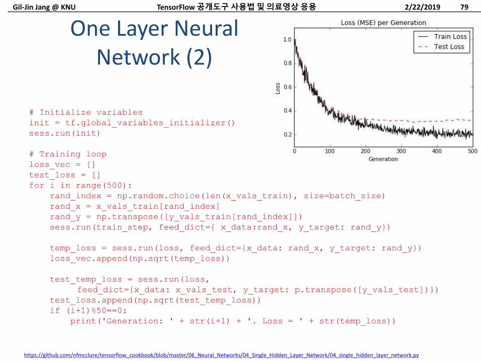
One Layer Neural Network (2)
# Initialize variables
init = tf.global_variables_initializer()
sess.run(init)
# Training loop
loss_vec = []
test_loss = []
for i in range(500):
rand_index = np.random.choice(len(x_vals_train), size=batch_size)
rand_x = x_vals_train[rand_index]
rand_y = np.transpose([y_vals_train[rand_index]])
sess.run(train_step, feed_dict={ x_data:rand_x, y_target: rand_y})
temp_loss = sess.run(loss, feed_dict={x_data: rand_x, y_target: rand_y})
loss_vec.append(np.sqrt(temp_loss))
test_temp_loss = sess.run(loss,
feed_dict={x_data: x_vals_test, y_target: p.transpose([y_vals_test])})
test_loss.append(np.sqrt(test_temp_loss))
if (i+1)%50==0:
print('Generation: ' + str(i+1) + '. Loss = ' + str(temp_loss))
2/22/2019TensorFlow 공개도구사용법및의료영상응용 79
https://github.com/nfmcclure/tensorflow_cookbook/blob/master/06_Neural_Networks/04_Single_Hidden_Layer_Network/04_single_hidden_layer_network.py
Gil-Jin Jang @ KNU
Create neural networks with three hidden layers.
Regression task:
– Predicting the birthweight in the low birthweight dataset.
– The low-birthweight dataset includes the actual birthweight and an indicator variable if the birthweight is above or below 2,500 grams.
– Target: actual birthweight (regression) and indicator variable (classification)
6.6 Using Multi-layer Neural Networks
2/22/2019TensorFlow 공개도구사용법및의료영상응용 80
Gil-Jin Jang @ KNU
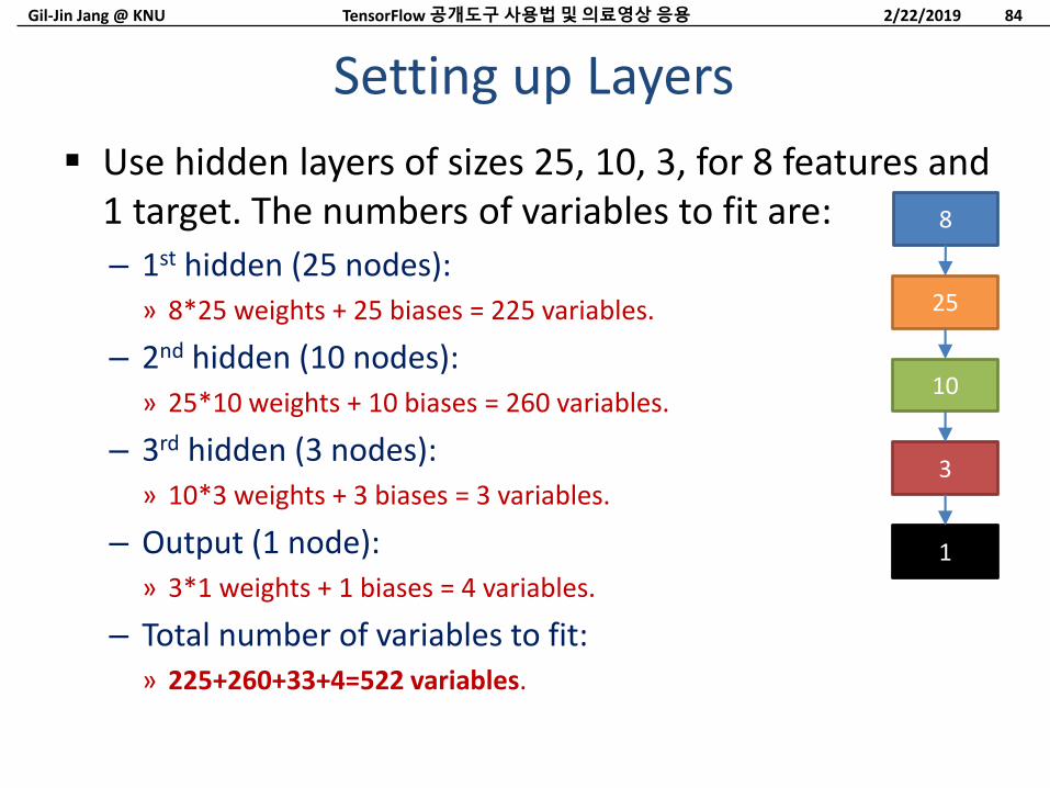
Use hidden layers of sizes 25, 10, 3, for 8 features and 1 target. The numbers of variables to fit are:
– 1st hidden (25 nodes):» 8*25 weights + 25 biases = 225 variables.
– 2nd hidden (10 nodes):» 25*10 weights + 10 biases = 260 variables.
– 3rd hidden (3 nodes):» 10*3 weights + 3 biases = 3 variables.
– Output (1 node):» 3*1 weights + 1 biases = 4 variables.
– Total number of variables to fit:» 225+260+33+4=522 variables.
Setting up Layers
2/22/2019TensorFlow 공개도구사용법및의료영상응용 84
8
25
10
3
1
Gil-Jin Jang @ KNU
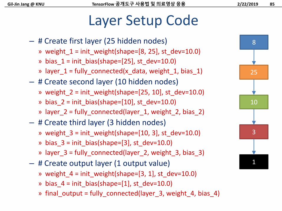
– # Create first layer (25 hidden nodes)» weight_1 = init_weight(shape=[8, 25], st_dev=10.0)
» bias_1 = init_bias(shape=[25], st_dev=10.0)
» layer_1 = fully_connected(x_data, weight_1, bias_1)
– # Create second layer (10 hidden nodes)» weight_2 = init_weight(shape=[25, 10], st_dev=10.0)
» bias_2 = init_bias(shape=[10], st_dev=10.0)
» layer_2 = fully_connected(layer_1, weight_2, bias_2)
– # Create third layer (3 hidden nodes)» weight_3 = init_weight(shape=[10, 3], st_dev=10.0)
» bias_3 = init_bias(shape=[3], st_dev=10.0)
» layer_3 = fully_connected(layer_2, weight_3, bias_3)
– # Create output layer (1 output value)» weight_4 = init_weight(shape=[3, 1], st_dev=10.0)
» bias_4 = init_bias(shape=[1], st_dev=10.0)
» final_output = fully_connected(layer_3, weight_4, bias_4)
Layer Setup Code
2/22/2019TensorFlow 공개도구사용법및의료영상응용 85
8
25
10
3
1
Gil-Jin Jang @ KNU
Running the Session and Results
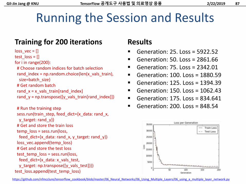
Training for 200 iterationsloss_vec = []test_loss = []for i in range(200):# Choose random indices for batch selectionrand_index = np.random.choice(len(x_vals_train),size=batch_size)
# Get random batchrand_x = x_vals_train[rand_index]rand_y = np.transpose([y_vals_train[rand_index]])
# Run the training stepsess.run(train_step, feed_dict={x_data: rand_x,y_target: rand_y})
# Get and store the train losstemp_loss = sess.run(loss,feed_dict={x_data: rand_x, y_target: rand_y})
loss_vec.append(temp_loss)# Get and store the test losstest_temp_loss = sess.run(loss,feed_dict={x_data: x_vals_test,y_target: np.transpose([y_vals_test])})
test_loss.append(test_temp_loss)
Results Generation: 25. Loss = 5922.52 Generation: 50. Loss = 2861.66 Generation: 75. Loss = 2342.01 Generation: 100. Loss = 1880.59 Generation: 125. Loss = 1394.39 Generation: 150. Loss = 1062.43 Generation: 175. Loss = 834.641 Generation: 200. Loss = 848.54
2/22/2019TensorFlow 공개도구사용법및의료영상응용 87
https://github.com/nfmcclure/tensorflow_cookbook/blob/master/06_Neural_Networks/06_Using_Multiple_Layers/06_using_a_multiple_layer_network.py
Gil-Jin Jang @ KNU
CHAPTER 8.CONVOLUTIONAL NEURAL NETWORKSOverview of the basic architecture
MNIST / CIFAR10 examples
Additional acknowledgments: Yann LeCun, Antonio Torralba, Boris Ginzburg
2/22/2019TensorFlow 공개도구사용법및의료영상응용 89
Gil-Jin Jang @ KNU
8.1 Introduction
8.2 Implementing a Simpler CNN (MNIST)
8.3 Implementing an Advanced CNN (CIFAR10)
8.4 Retraining an Existing Architecture.
8.5 Using Stylenet/NeuralStyle.
8.6 Implementing Deep Dream.
8. Convolutional Neural Networks
2/22/2019TensorFlow 공개도구사용법및의료영상응용 90
Gil-Jin Jang @ KNU
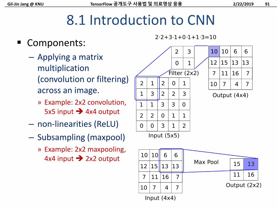
Components:
– Applying a matrix multiplication (convolution or filtering) across an image.» Example: 2x2 convolution,
5x5 input 4x4 output
– non-linearities (ReLU)
– Subsampling (maxpool)» Example: 2x2 maxpooling,
4x4 input 2x2 output
8.1 Introduction to CNN
2/22/2019TensorFlow 공개도구사용법및의료영상응용 91
Gil-Jin Jang @ KNU
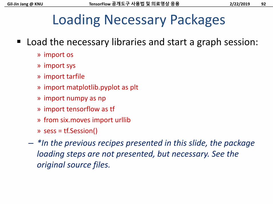
Load the necessary libraries and start a graph session:» import os
» import sys
» import tarfile
» import matplotlib.pyplot as plt
» import numpy as np
» import tensorflow as tf
» from six.moves import urllib
» sess = tf.Session()
– *In the previous recipes presented in this slide, the package loading steps are not presented, but necessary. See the original source files.
Loading Necessary Packages
2/22/2019TensorFlow 공개도구사용법및의료영상응용 92
Gil-Jin Jang @ KNU
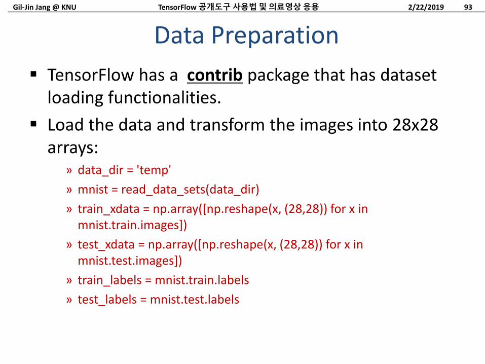
TensorFlow has a contrib package that has dataset loading functionalities.
Load the data and transform the images into 28x28 arrays:
» data_dir = 'temp'
» mnist = read_data_sets(data_dir)
» train_xdata = np.array([np.reshape(x, (28,28)) for x in mnist.train.images])
» test_xdata = np.array([np.reshape(x, (28,28)) for x in mnist.test.images])
» train_labels = mnist.train.labels
» test_labels = mnist.test.labels
Data Preparation
2/22/2019TensorFlow 공개도구사용법및의료영상응용 93
Gil-Jin Jang @ KNU
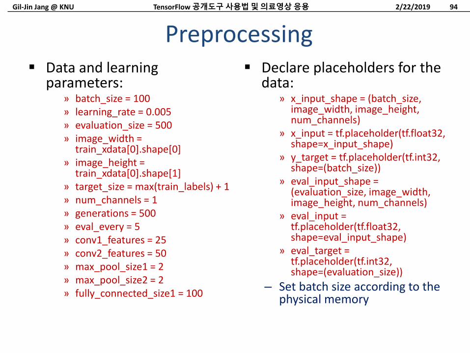
Preprocessing Data and learning
parameters:» batch_size = 100» learning_rate = 0.005» evaluation_size = 500» image_width =
train_xdata[0].shape[0]» image_height =
train_xdata[0].shape[1]» target_size = max(train_labels) + 1» num_channels = 1» generations = 500» eval_every = 5» conv1_features = 25» conv2_features = 50» max_pool_size1 = 2» max_pool_size2 = 2» fully_connected_size1 = 100
Declare placeholders for the data:
» x_input_shape = (batch_size, image_width, image_height, num_channels)
» x_input = tf.placeholder(tf.float32, shape=x_input_shape)
» y_target = tf.placeholder(tf.int32, shape=(batch_size))
» eval_input_shape = (evaluation_size, image_width, image_height, num_channels)
» eval_input = tf.placeholder(tf.float32, shape=eval_input_shape)
» eval_target = tf.placeholder(tf.int32, shape=(evaluation_size))
– Set batch size according to the physical memory
2/22/2019TensorFlow 공개도구사용법및의료영상응용 94
Gil-Jin Jang @ KNU
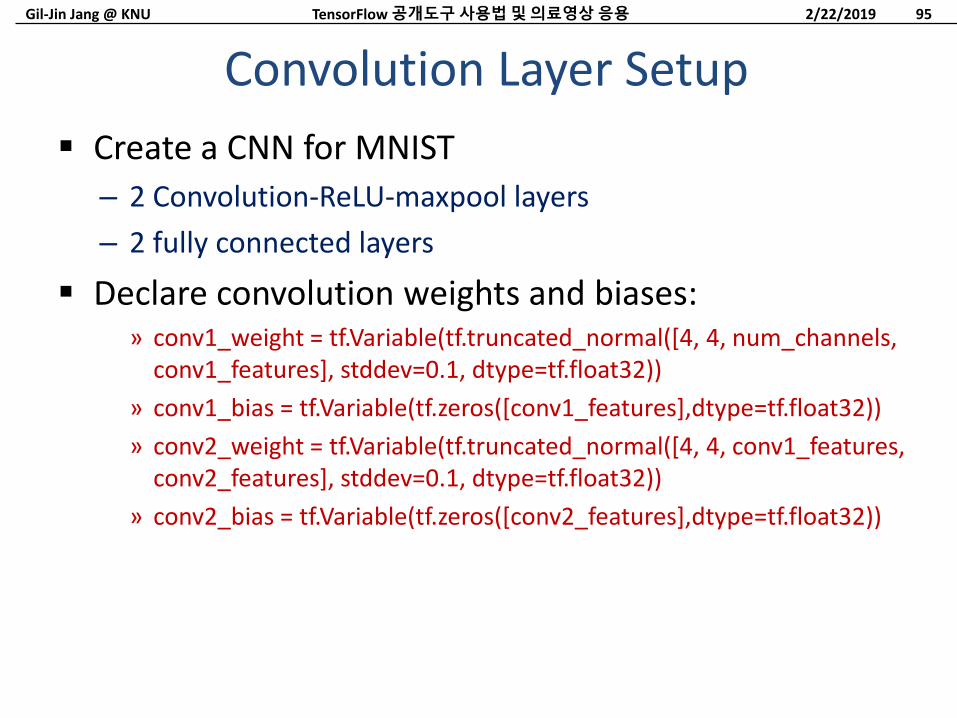
Create a CNN for MNIST
– 2 Convolution-ReLU-maxpool layers
– 2 fully connected layers
Declare convolution weights and biases:» conv1_weight = tf.Variable(tf.truncated_normal([4, 4, num_channels,
conv1_features], stddev=0.1, dtype=tf.float32))
» conv1_bias = tf.Variable(tf.zeros([conv1_features],dtype=tf.float32))
» conv2_weight = tf.Variable(tf.truncated_normal([4, 4, conv1_features, conv2_features], stddev=0.1, dtype=tf.float32))
» conv2_bias = tf.Variable(tf.zeros([conv2_features],dtype=tf.float32))
Convolution Layer Setup
2/22/2019TensorFlow 공개도구사용법및의료영상응용 95
Gil-Jin Jang @ KNU
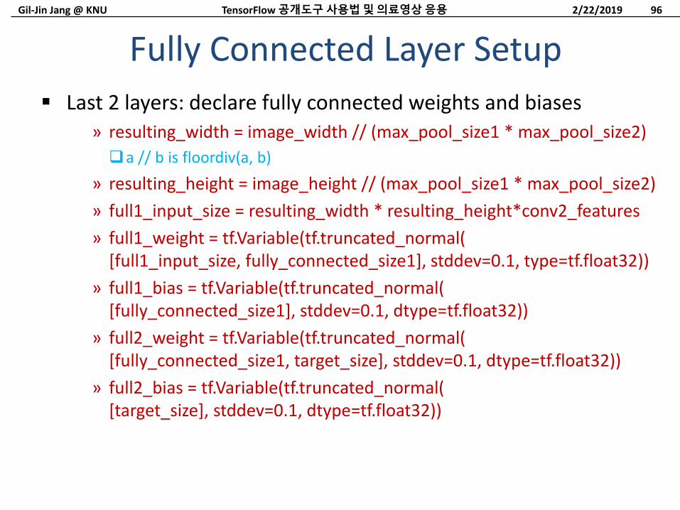
Last 2 layers: declare fully connected weights and biases» resulting_width = image_width // (max_pool_size1 * max_pool_size2)
a // b is floordiv(a, b)
» resulting_height = image_height // (max_pool_size1 * max_pool_size2)
» full1_input_size = resulting_width * resulting_height*conv2_features
» full1_weight = tf.Variable(tf.truncated_normal([full1_input_size, fully_connected_size1], stddev=0.1, type=tf.float32))
» full1_bias = tf.Variable(tf.truncated_normal([fully_connected_size1], stddev=0.1, dtype=tf.float32))
» full2_weight = tf.Variable(tf.truncated_normal([fully_connected_size1, target_size], stddev=0.1, dtype=tf.float32))
» full2_bias = tf.Variable(tf.truncated_normal([target_size], stddev=0.1, dtype=tf.float32))
Fully Connected Layer Setup
2/22/2019TensorFlow 공개도구사용법및의료영상응용 96
Gil-Jin Jang @ KNU
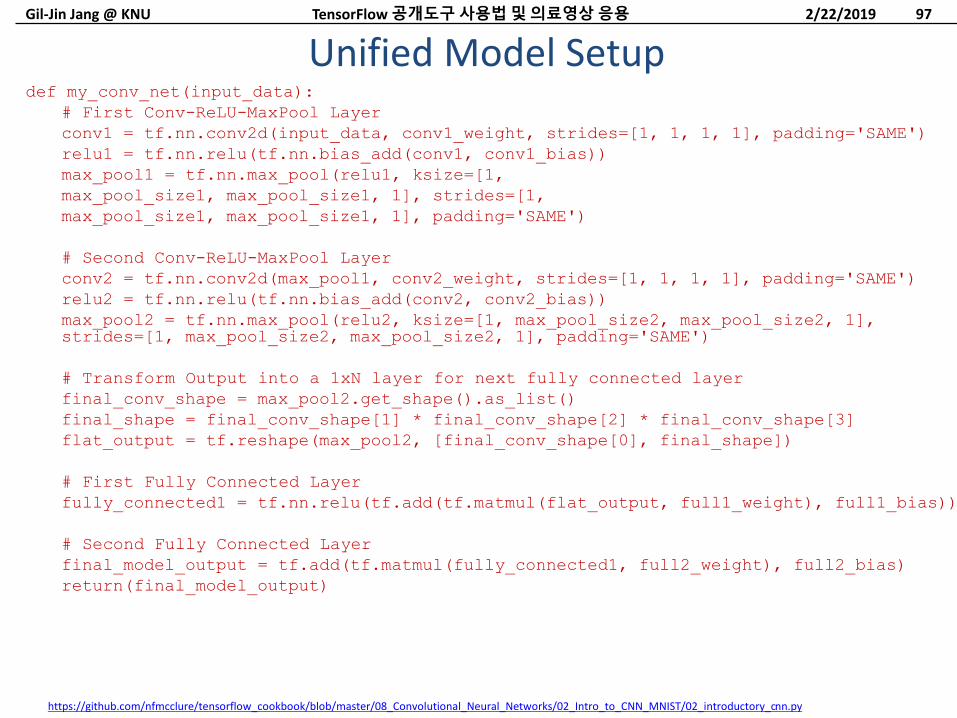
def my_conv_net(input_data):
# First Conv-ReLU-MaxPool Layer
conv1 = tf.nn.conv2d(input_data, conv1_weight, strides=[1, 1, 1, 1], padding='SAME')
relu1 = tf.nn.relu(tf.nn.bias_add(conv1, conv1_bias))
max_pool1 = tf.nn.max_pool(relu1, ksize=[1,
max_pool_size1, max_pool_size1, 1], strides=[1,
max_pool_size1, max_pool_size1, 1], padding='SAME')
# Second Conv-ReLU-MaxPool Layer
conv2 = tf.nn.conv2d(max_pool1, conv2_weight, strides=[1, 1, 1, 1], padding='SAME')
relu2 = tf.nn.relu(tf.nn.bias_add(conv2, conv2_bias))
max_pool2 = tf.nn.max_pool(relu2, ksize=[1, max_pool_size2, max_pool_size2, 1], strides=[1, max_pool_size2, max_pool_size2, 1], padding='SAME')
# Transform Output into a 1xN layer for next fully connected layer
final_conv_shape = max_pool2.get_shape().as_list()
final_shape = final_conv_shape[1] * final_conv_shape[2] * final_conv_shape[3]
flat_output = tf.reshape(max_pool2, [final_conv_shape[0], final_shape])
# First Fully Connected Layer
fully_connected1 = tf.nn.relu(tf.add(tf.matmul(flat_output, full1_weight), full1_bias))
# Second Fully Connected Layer
final_model_output = tf.add(tf.matmul(fully_connected1, full2_weight), full2_bias)
return(final_model_output)
Unified Model Setup2/22/2019TensorFlow 공개도구사용법및의료영상응용 97
https://github.com/nfmcclure/tensorflow_cookbook/blob/master/08_Convolutional_Neural_Networks/02_Intro_to_CNN_MNIST/02_introductory_cnn.py
Gil-Jin Jang @ KNU
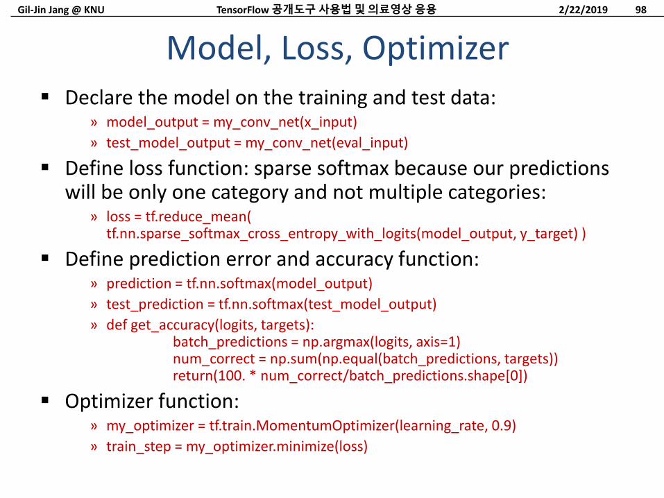
Declare the model on the training and test data:» model_output = my_conv_net(x_input)
» test_model_output = my_conv_net(eval_input)
Define loss function: sparse softmax because our predictions will be only one category and not multiple categories:
» loss = tf.reduce_mean(tf.nn.sparse_softmax_cross_entropy_with_logits(model_output, y_target) )
Define prediction error and accuracy function:» prediction = tf.nn.softmax(model_output)
» test_prediction = tf.nn.softmax(test_model_output)
» def get_accuracy(logits, targets):batch_predictions = np.argmax(logits, axis=1)num_correct = np.sum(np.equal(batch_predictions, targets))return(100. * num_correct/batch_predictions.shape[0])
Optimizer function:» my_optimizer = tf.train.MomentumOptimizer(learning_rate, 0.9)
» train_step = my_optimizer.minimize(loss)
Model, Loss, Optimizer
2/22/2019TensorFlow 공개도구사용법및의료영상응용 98
Gil-Jin Jang @ KNU
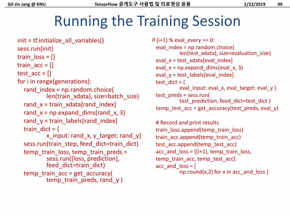
Running the Training Sessioninit = tf.initialize_all_variables()sess.run(init)train_loss = []train_acc = []test_acc = []for i in range(generations):
rand_index = np.random.choice(len(train_xdata), size=batch_size)
rand_x = train_xdata[rand_index]rand_x = np.expand_dims(rand_x, 3)rand_y = train_labels[rand_index]train_dict = {
x_input: rand_x, y_target: rand_y}sess.run(train_step, feed_dict=train_dict)temp_train_loss, temp_train_preds =
sess.run([loss, prediction],feed_dict=train_dict)
temp_train_acc = get_accuracy(temp_train_preds, rand_y )
if (i+1) % eval_every == 0:eval_index = np.random.choice(
len(test_xdata), size=evaluation_size)eval_x = test_xdata[eval_index]eval_x = np.expand_dims(eval_x, 3)eval_y = test_labels[eval_index]test_dict = {
eval_input: eval_x, eval_target: eval_y }test_preds = sess.run(
test_prediction, feed_dict=test_dict )temp_test_acc = get_accuracy(test_preds, eval_y)
# Record and print resultstrain_loss.append(temp_train_loss)train_acc.append(temp_train_acc)test_acc.append(temp_test_acc)acc_and_loss = [(i+1), temp_train_loss,temp_train_acc, temp_test_acc]acc_and_loss = [
np.round(x,2) for x in acc_and_loss ]
2/22/2019TensorFlow 공개도구사용법및의료영상응용 99
Gil-Jin Jang @ KNU
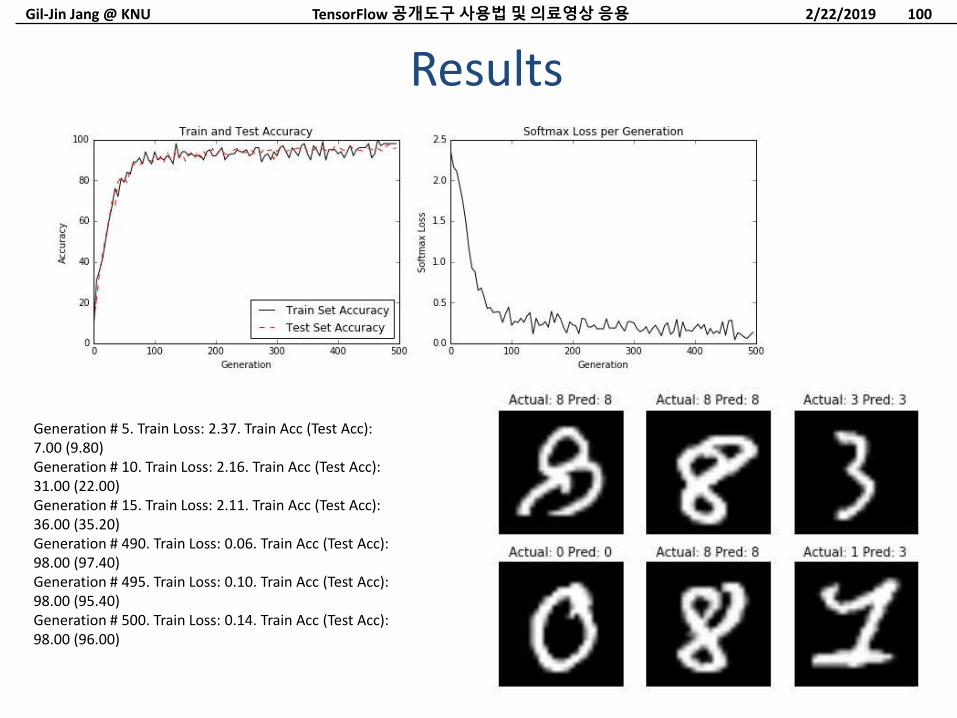
Results
2/22/2019TensorFlow 공개도구사용법및의료영상응용 100
Generation # 5. Train Loss: 2.37. Train Acc (Test Acc):7.00 (9.80)Generation # 10. Train Loss: 2.16. Train Acc (Test Acc):31.00 (22.00)Generation # 15. Train Loss: 2.11. Train Acc (Test Acc):36.00 (35.20)Generation # 490. Train Loss: 0.06. Train Acc (Test Acc):98.00 (97.40)Generation # 495. Train Loss: 0.10. Train Acc (Test Acc):98.00 (95.40)Generation # 500. Train Loss: 0.14. Train Acc (Test Acc):98.00 (96.00)
Gil-Jin Jang @ KNU
Full code is available at:– https://github.com/nfmcclure/tensorflow_cookbook/blob/master
/08_Convolutional_Neural_Networks/02_Intro_to_CNN_MNIST/02_introductory_cnn.py
The accuracy of the prediction may increase as the depth of the network gets deeper– Repeat the convolution, maxpool, ReLU series until the
satisfactory performance is obtained» Note: the order of maxpool and ReLU is not important, because ReLU is a
monotonically increasing function
– Enough data to reliably train the model parameters» Determining the proper number of training samples is a hard question: do
it in a trial-and-error fashion
» Try with lower learning rate and obtain the BEST depth, and gradually increase the learning rate
More Resources
2/22/2019TensorFlow 공개도구사용법및의료영상응용 101
Gil-Jin Jang @ KNU
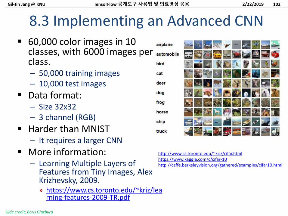
60,000 color images in 10 classes, with 6000 images per class.– 50,000 training images– 10,000 test images
Data format:– Size 32x32– 3 channel (RGB)
Harder than MNIST– It requires a larger CNN
More information:– Learning Multiple Layers of
Features from Tiny Images, Alex Krizhevsky, 2009.» https://www.cs.toronto.edu/~kriz/lea
rning-features-2009-TR.pdf
8.3 Implementing an Advanced CNN
2/22/2019TensorFlow 공개도구사용법및의료영상응용 102
Slide credit: Boris Ginzburg
http://www.cs.toronto.edu/~kriz/cifar.htmlhttps://www.kaggle.com/c/cifar-10http://caffe.berkeleyvision.org/gathered/examples/cifar10.html
Gil-Jin Jang @ KNU
– Set up the data directory and the URL to download the CIFAR-10 images:» data_dir = 'temp'
» if not os.path.exists(data_dir): os.makedirs(data_dir)
» cifar10_url = 'http://www.cs.toronto.edu/~kriz/cifar-10-binary.tar.gz'
» data_file = os.path.join(data_dir, 'cifar-10-binary.tar.gz')
– Load file» if not os.path.isfile(data_file):
» filepath, _ = urllib.request.urlretrieve(cifar10_url,data_file, progress)
– Extract file» tarfile.open(filepath, 'r:gz').extractall(data_dir)
Loading Data
2/22/2019TensorFlow 공개도구사용법및의료영상응용 103
Gil-Jin Jang @ KNU
Set up parameters to read in the binary CIFAR-10 images:
» image_vec_length = image_height * image_width * num_channels
» record_length = 1 + image_vec_length
Function read_cifar_files():
– Sets up record reader and returns a randomly distorted image» Declare a record reader object that will read in a fixed length of bytes.
» Split apart the image and label.
» Randomly distort the image with TensorFlow's built in image modification functions:
Data Preparation
2/22/2019TensorFlow 공개도구사용법및의료영상응용 104
Gil-Jin Jang @ KNU
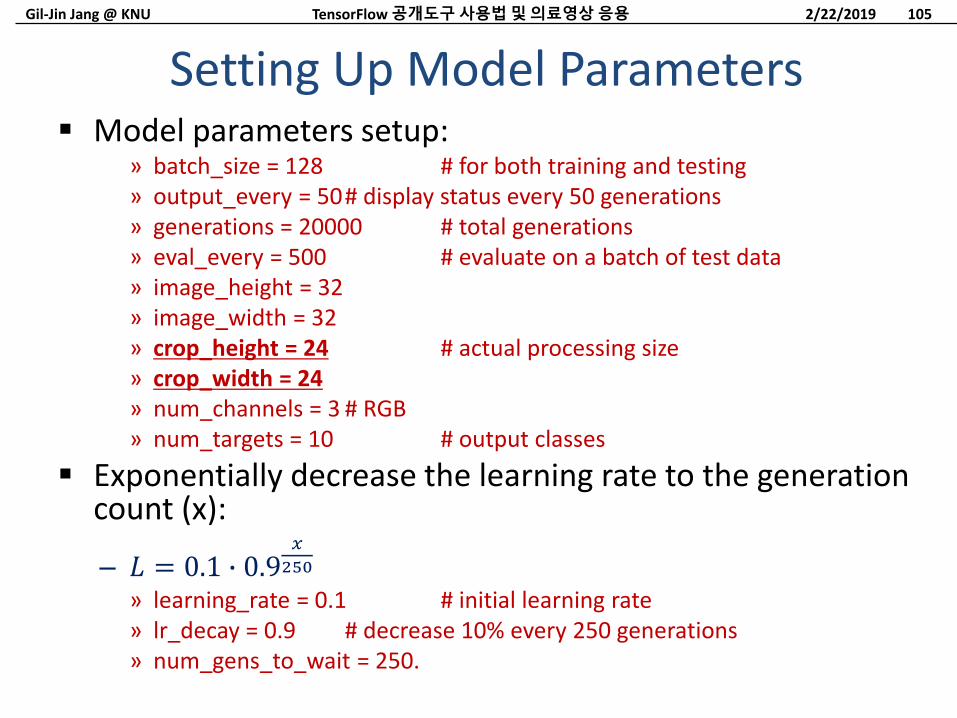
Model parameters setup:» batch_size = 128 # for both training and testing» output_every = 50# display status every 50 generations» generations = 20000 # total generations» eval_every = 500 # evaluate on a batch of test data» image_height = 32» image_width = 32» crop_height = 24 # actual processing size» crop_width = 24» num_channels = 3 # RGB» num_targets = 10 # output classes
Exponentially decrease the learning rate to the generation count (x):
– 𝐿 = 0.1 ∙ 0.9𝑥
250
» learning_rate = 0.1 # initial learning rate» lr_decay = 0.9 # decrease 10% every 250 generations» num_gens_to_wait = 250.
Setting Up Model Parameters
2/22/2019TensorFlow 공개도구사용법및의료영상응용 105
Gil-Jin Jang @ KNU
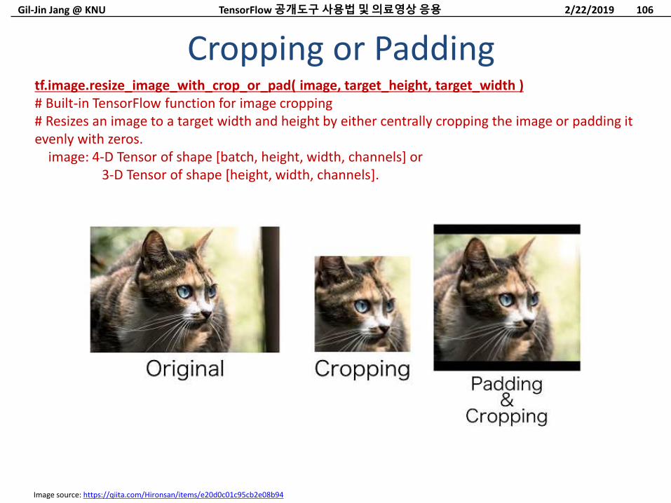
Cropping or Padding
2/22/2019TensorFlow 공개도구사용법및의료영상응용 106
tf.image.resize_image_with_crop_or_pad( image, target_height, target_width )# Built-in TensorFlow function for image cropping# Resizes an image to a target width and height by either centrally cropping the image or padding it evenly with zeros.
image: 4-D Tensor of shape [batch, height, width, channels] or 3-D Tensor of shape [height, width, channels].
Image source: https://qiita.com/Hironsan/items/e20d0c01c95cb2e08b94
Gil-Jin Jang @ KNU
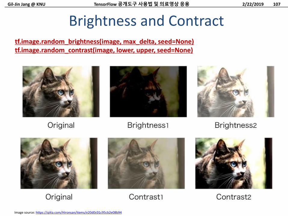
Brightness and Contract
2/22/2019TensorFlow 공개도구사용법및의료영상응용 107
tf.image.random_brightness(image, max_delta, seed=None)tf.image.random_contrast(image, lower, upper, seed=None)
Image source: https://qiita.com/Hironsan/items/e20d0c01c95cb2e08b94
Gil-Jin Jang @ KNU
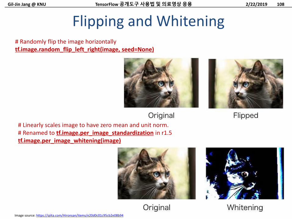
Flipping and Whitening
2/22/2019TensorFlow 공개도구사용법및의료영상응용 108
# Randomly flip the image horizontallytf.image.random_flip_left_right(image, seed=None)
Image source: https://qiita.com/Hironsan/items/e20d0c01c95cb2e08b94
# Linearly scales image to have zero mean and unit norm.# Renamed to tf.image.per_image_standardization in r1.5tf.image.per_image_whitening(image)
Gil-Jin Jang @ KNU
Random Cropping
2/22/2019TensorFlow 공개도구사용법및의료영상응용 109
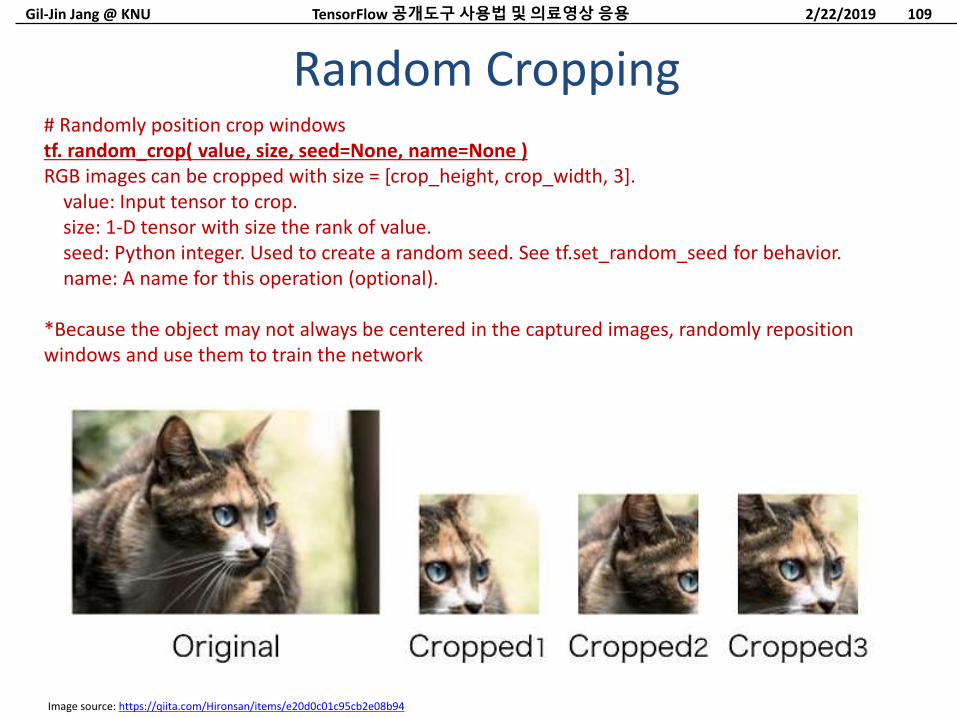
# Randomly position crop windowstf. random_crop( value, size, seed=None, name=None )RGB images can be cropped with size = [crop_height, crop_width, 3].
value: Input tensor to crop.size: 1-D tensor with size the rank of value.seed: Python integer. Used to create a random seed. See tf.set_random_seed for behavior.name: A name for this operation (optional).
*Because the object may not always be centered in the captured images, randomly reposition windows and use them to train the network
Image source: https://qiita.com/Hironsan/items/e20d0c01c95cb2e08b94
Gil-Jin Jang @ KNU 2/22/2019TensorFlow 공개도구사용법및의료영상응용 110
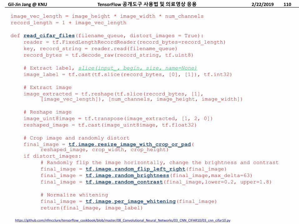
image_vec_length = image_height * image_width * num_channels
record_length = 1 + image_vec_length
def read_cifar_files(filename_queue, distort_images = True):
reader = tf.FixedLengthRecordReader(record_bytes=record_length)
key, record_string = reader.read(filename_queue)
record_bytes = tf.decode_raw(record_string, tf.uint8)
# Extract label, slice(input_, begin, size, name=None)
image_label = tf.cast(tf.slice(record_bytes, [0], [1]), tf.int32)
# Extract image
image_extracted = tf.reshape(tf.slice(record_bytes, [1],[image_vec_length]), [num_channels, image_height, image_width])
# Reshape image
image_uint8image = tf.transpose(image_extracted, [1, 2, 0])
reshaped_image = tf.cast(image_uint8image, tf.float32)
# Crop image and randomly distort
final_image = tf.image.resize_image_with_crop_or_pad(reshaped_image, crop_width, crop_height)
if distort_images:
# Randomly flip the image horizontally, change the brightness and contrast
final_image = tf.image.random_flip_left_right(final_image)
final_image = tf.image.random_brightness(final_image,max_delta=63)
final_image = tf.image.random_contrast(final_image,lower=0.2, upper=1.8)
# Normalize whitening
final_image = tf.image.per_image_whitening(final_image)
return(final_image, image_label)
https://github.com/nfmcclure/tensorflow_cookbook/blob/master/08_Convolutional_Neural_Networks/03_CNN_CIFAR10/03_cnn_cifar10.py
Gil-Jin Jang @ KNU
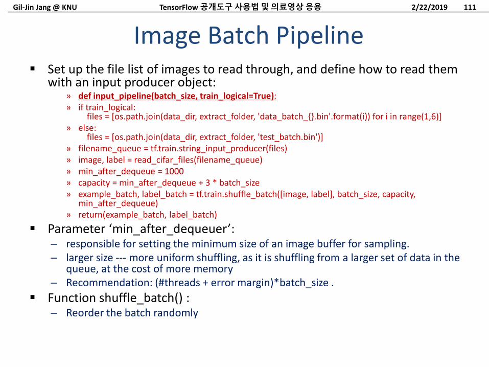
Set up the file list of images to read through, and define how to read them with an input producer object:
» def input_pipeline(batch_size, train_logical=True):» if train_logical:
files = [os.path.join(data_dir, extract_folder, 'data_batch_{}.bin'.format(i)) for i in range(1,6)]» else:
files = [os.path.join(data_dir, extract_folder, 'test_batch.bin')]» filename_queue = tf.train.string_input_producer(files)» image, label = read_cifar_files(filename_queue)» min_after_dequeue = 1000» capacity = min_after_dequeue + 3 * batch_size» example_batch, label_batch = tf.train.shuffle_batch([image, label], batch_size, capacity,
min_after_dequeue)» return(example_batch, label_batch)
Parameter ‘min_after_dequeuer’:– responsible for setting the minimum size of an image buffer for sampling.– larger size --- more uniform shuffling, as it is shuffling from a larger set of data in the
queue, at the cost of more memory– Recommendation: (#threads + error margin)*batch_size .
Function shuffle_batch() :– Reorder the batch randomly
Image Batch Pipeline
2/22/2019TensorFlow 공개도구사용법및의료영상응용 111
Gil-Jin Jang @ KNU
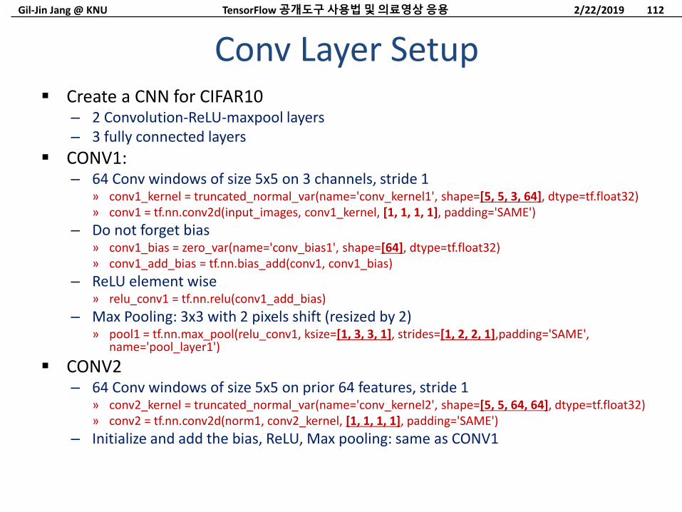
Create a CNN for CIFAR10– 2 Convolution-ReLU-maxpool layers– 3 fully connected layers
CONV1:– 64 Conv windows of size 5x5 on 3 channels, stride 1
» conv1_kernel = truncated_normal_var(name='conv_kernel1', shape=[5, 5, 3, 64], dtype=tf.float32)» conv1 = tf.nn.conv2d(input_images, conv1_kernel, [1, 1, 1, 1], padding='SAME')
– Do not forget bias» conv1_bias = zero_var(name='conv_bias1', shape=[64], dtype=tf.float32)» conv1_add_bias = tf.nn.bias_add(conv1, conv1_bias)
– ReLU element wise» relu_conv1 = tf.nn.relu(conv1_add_bias)
– Max Pooling: 3x3 with 2 pixels shift (resized by 2)» pool1 = tf.nn.max_pool(relu_conv1, ksize=[1, 3, 3, 1], strides=[1, 2, 2, 1],padding='SAME',
name='pool_layer1')
CONV2– 64 Conv windows of size 5x5 on prior 64 features, stride 1
» conv2_kernel = truncated_normal_var(name='conv_kernel2', shape=[5, 5, 64, 64], dtype=tf.float32)» conv2 = tf.nn.conv2d(norm1, conv2_kernel, [1, 1, 1, 1], padding='SAME')
– Initialize and add the bias, ReLU, Max pooling: same as CONV1
Conv Layer Setup
2/22/2019TensorFlow 공개도구사용법및의료영상응용 112
Gil-Jin Jang @ KNU
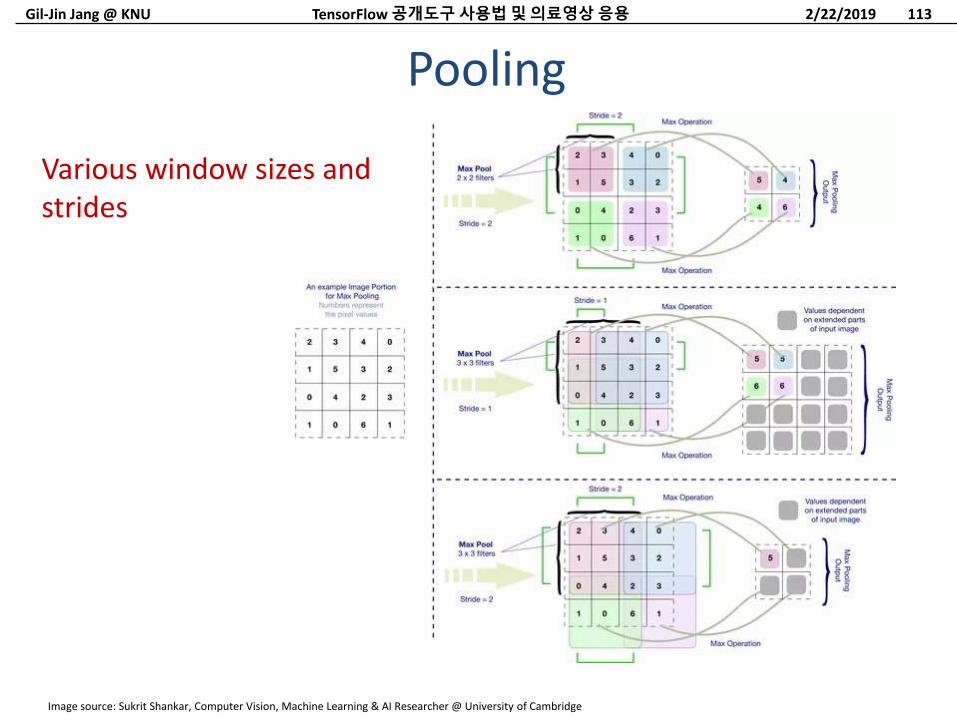
Pooling
2/22/2019TensorFlow 공개도구사용법및의료영상응용 113
Various window sizes and strides
Image source: Sukrit Shankar, Computer Vision, Machine Learning & AI Researcher @ University of Cambridge
Gil-Jin Jang @ KNU
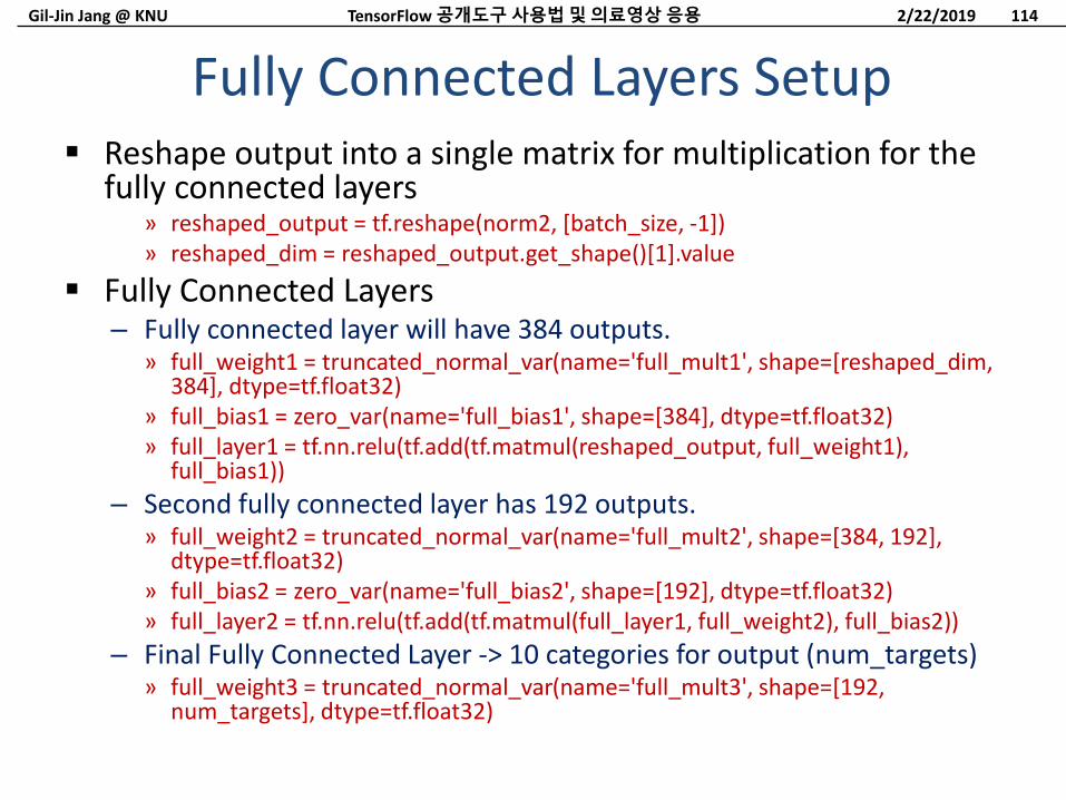
Reshape output into a single matrix for multiplication for the fully connected layers
» reshaped_output = tf.reshape(norm2, [batch_size, -1])» reshaped_dim = reshaped_output.get_shape()[1].value
Fully Connected Layers– Fully connected layer will have 384 outputs.
» full_weight1 = truncated_normal_var(name='full_mult1', shape=[reshaped_dim, 384], dtype=tf.float32)
» full_bias1 = zero_var(name='full_bias1', shape=[384], dtype=tf.float32)» full_layer1 = tf.nn.relu(tf.add(tf.matmul(reshaped_output, full_weight1),
full_bias1))
– Second fully connected layer has 192 outputs.» full_weight2 = truncated_normal_var(name='full_mult2', shape=[384, 192],
dtype=tf.float32)» full_bias2 = zero_var(name='full_bias2', shape=[192], dtype=tf.float32)» full_layer2 = tf.nn.relu(tf.add(tf.matmul(full_layer1, full_weight2), full_bias2))
– Final Fully Connected Layer -> 10 categories for output (num_targets)» full_weight3 = truncated_normal_var(name='full_mult3', shape=[192,
num_targets], dtype=tf.float32)
Fully Connected Layers Setup
2/22/2019TensorFlow 공개도구사용법및의료영상응용 114
Gil-Jin Jang @ KNU
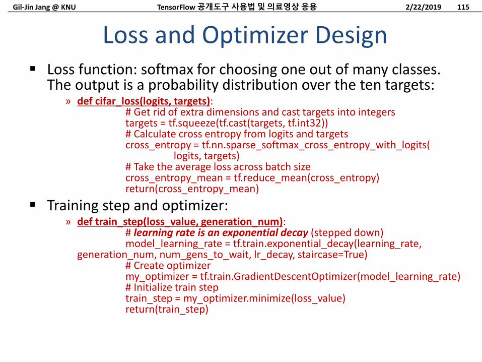
Loss function: softmax for choosing one out of many classes. The output is a probability distribution over the ten targets:
» def cifar_loss(logits, targets):# Get rid of extra dimensions and cast targets into integerstargets = tf.squeeze(tf.cast(targets, tf.int32))# Calculate cross entropy from logits and targetscross_entropy = tf.nn.sparse_softmax_cross_entropy_with_logits(
logits, targets)# Take the average loss across batch sizecross_entropy_mean = tf.reduce_mean(cross_entropy)return(cross_entropy_mean)
Training step and optimizer:» def train_step(loss_value, generation_num):
# learning rate is an exponential decay (stepped down)model_learning_rate = tf.train.exponential_decay(learning_rate,
generation_num, num_gens_to_wait, lr_decay, staircase=True)# Create optimizermy_optimizer = tf.train.GradientDescentOptimizer(model_learning_rate)# Initialize train steptrain_step = my_optimizer.minimize(loss_value)return(train_step)
Loss and Optimizer Design
2/22/2019TensorFlow 공개도구사용법및의료영상응용 115
Gil-Jin Jang @ KNU
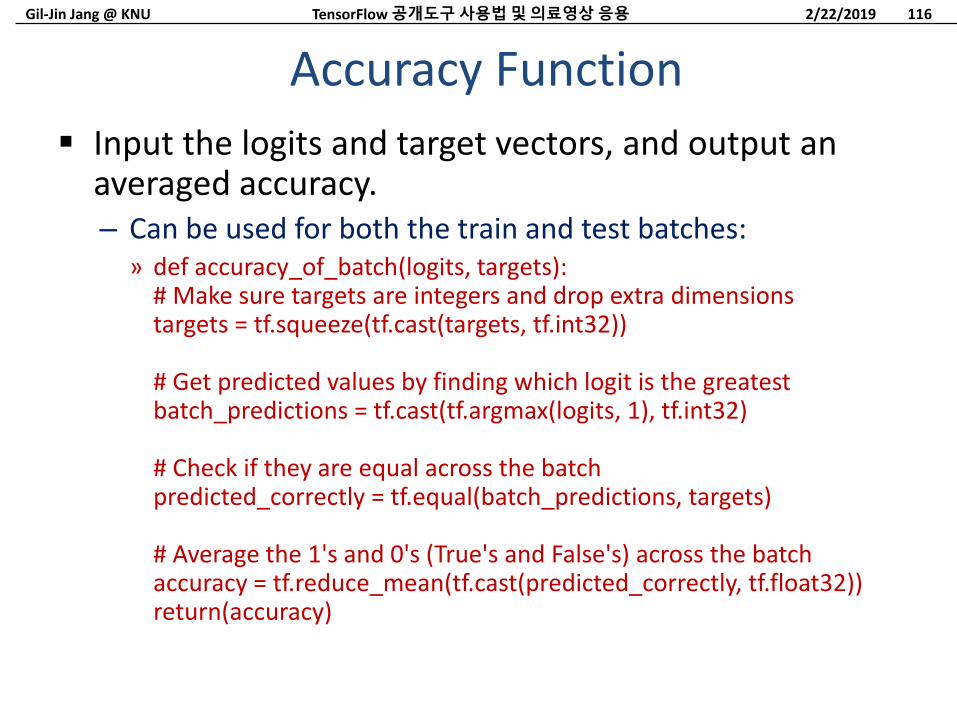
Input the logits and target vectors, and output an averaged accuracy.– Can be used for both the train and test batches:
» def accuracy_of_batch(logits, targets):# Make sure targets are integers and drop extra dimensionstargets = tf.squeeze(tf.cast(targets, tf.int32))
# Get predicted values by finding which logit is the greatestbatch_predictions = tf.cast(tf.argmax(logits, 1), tf.int32)
# Check if they are equal across the batchpredicted_correctly = tf.equal(batch_predictions, targets)
# Average the 1's and 0's (True's and False's) across the batchaccuracy = tf.reduce_mean(tf.cast(predicted_correctly, tf.float32))return(accuracy)
Accuracy Function
2/22/2019TensorFlow 공개도구사용법및의료영상응용 116
Gil-Jin Jang @ KNU
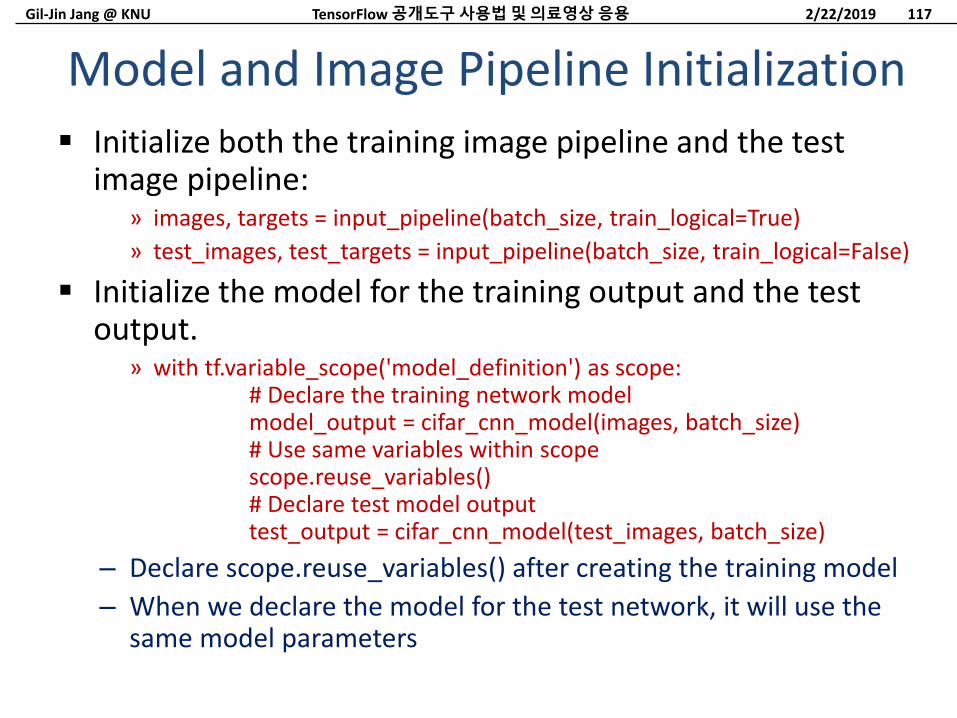
Initialize both the training image pipeline and the test image pipeline:
» images, targets = input_pipeline(batch_size, train_logical=True)
» test_images, test_targets = input_pipeline(batch_size, train_logical=False)
Initialize the model for the training output and the test output.
» with tf.variable_scope('model_definition') as scope:# Declare the training network modelmodel_output = cifar_cnn_model(images, batch_size)# Use same variables within scopescope.reuse_variables()# Declare test model outputtest_output = cifar_cnn_model(test_images, batch_size)
– Declare scope.reuse_variables() after creating the training model
– When we declare the model for the test network, it will use the same model parameters
Model and Image Pipeline Initialization
2/22/2019TensorFlow 공개도구사용법및의료영상응용 117
Gil-Jin Jang @ KNU
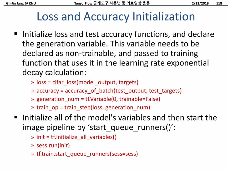
Initialize loss and test accuracy functions, and declare the generation variable. This variable needs to be declared as non-trainable, and passed to training function that uses it in the learning rate exponential decay calculation:
» loss = cifar_loss(model_output, targets)
» accuracy = accuracy_of_batch(test_output, test_targets)
» generation_num = tf.Variable(0, trainable=False)
» train_op = train_step(loss, generation_num)
Initialize all of the model's variables and then start the image pipeline by ‘start_queue_runners()’:
» init = tf.initialize_all_variables()
» sess.run(init)
» tf.train.start_queue_runners(sess=sess)
Loss and Accuracy Initialization
2/22/2019TensorFlow 공개도구사용법및의료영상응용 118
Gil-Jin Jang @ KNU
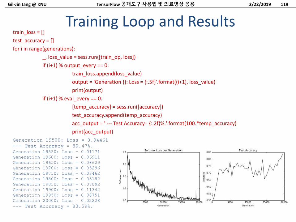
train_loss = []
test_accuracy = []
for i in range(generations):
_, loss_value = sess.run([train_op, loss])
if (i+1) % output_every == 0:
train_loss.append(loss_value)
output = 'Generation {}: Loss = {:.5f}'.format((i+1), loss_value)
print(output)
if (i+1) % eval_every == 0:
[temp_accuracy] = sess.run([accuracy])
test_accuracy.append(temp_accuracy)
acc_output = ' --- Test Accuracy= {:.2f}%.'.format(100.*temp_accuracy)
print(acc_output)
Training Loop and Results
2/22/2019TensorFlow 공개도구사용법및의료영상응용 119
Generation 19500: Loss = 0.04461
--- Test Accuracy = 80.47%.
Generation 19550: Loss = 0.01171
Generation 19600: Loss = 0.06911
Generation 19650: Loss = 0.08629
Generation 19700: Loss = 0.05296
Generation 19750: Loss = 0.03462
Generation 19800: Loss = 0.03182
Generation 19850: Loss = 0.07092
Generation 19900: Loss = 0.11342
Generation 19950: Loss = 0.08751
Generation 20000: Loss = 0.02228
--- Test Accuracy = 83.59%.
Gil-Jin Jang @ KNU
Numerous recipes from
– TensorFlow Machine Learning Cookbook. Nick McClure. Packt Publishing. ISBN 978-1-78646-216-9.
– Recipes available online» http://www.packtpub.com/
» https://github.com/nfmcclure/tensorflow_cookbook
ConclusionTensorFlow 공개도구사용법및의료영상응용 1202/22/2019
Gil-Jin Jang @ KNU
DEEP LEARNING ON MEDICAL IMAGE UNDERSTANDING
2/22/2019TensorFlow 공개도구사용법및의료영상응용 121
Gil-Jin Jang @ KNU
References– An Introduction to Biomedical Image Analysis with
TensorFlow and DLTK. Martin Rajchl. https://medium.com/tensorflow/an-introduction-to-biomedical-image-analysis-with-tensorflow-and-dltk-2c25304e7c13
– DLTK: State of the Art Reference Implementations for Deep Learning on Medical Images. Nick Pawlowski, Sofia Ira Ktena, Matthew C.H. Lee, Bernhard Kainz, Daniel Rueckert, Ben Glocker, Martin Rajchl. https://arxiv.org/abs/1711.06853Follow
DLTK: Deep Learning on Medical Imaging
2/22/2019TensorFlow 공개도구사용법및의료영상응용 122
Gil-Jin Jang @ KNU
Biomedical images are measurements of the human body
– Scales: microscopic, macroscopic, etc.
– Modalities: CT, PET, fMRI, ultrasound, etc.
Usually interpreted by domain experts (radiologist) for clinical tasks such as disease diagnosis
Biomedical Image Analysis
2/22/2019TensorFlow 공개도구사용법및의료영상응용 123
Gil-Jin Jang @ KNU
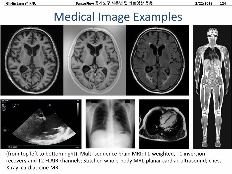
Medical Image Examples
2/22/2019TensorFlow 공개도구사용법및의료영상응용 124
(from top left to bottom right): Multi-sequence brain MRI: T1-weighted, T1 inversion recovery and T2 FLAIR channels; Stitched whole-body MRI; planar cardiac ultrasound; chest X-ray; cardiac cine MRI.
Gil-Jin Jang @ KNU
DLTK extends TensorFlow to enable deep learning on biomedical images
Provides specialty operations and functions, implementations of models, tutorials and code examples for typical applications.– https://github.com/DLTK/DLTK/tree/master/examples/tutori
als
– https://github.com/DLTK/DLTK/tree/master/examples/applications
Due to the different nature of acquisition, some images require special pre-processing– intensity normalization, bias-field correction, de-noising,
spatial normalization/registration, etc.
DLTK Basics
2/22/2019TensorFlow 공개도구사용법및의료영상응용 125
Gil-Jin Jang @ KNU
NifTI (.nii format)– Originally developed for brain imaging, but widely used for most other
volume images
NifTI header– Dimensions and size (store information about how to reconstruct the
image)
– Data type
– Voxel spacing (also the physical dimensions of voxels, typically in mm)
– Physical coordinate system origin
– Direction
Tensorflow trains the network in the space of voxels– Creates tensors of shape and dimensions [batch_size, dx, dy, dz, channels/features]
– Feature extractors (convolutional layers) assumes that voxel dimensions are isotropic (same in each dimension) and all images are oriented the same way
DLTK File Formats
2/22/2019TensorFlow 공개도구사용법및의료영상응용 126
Gil-Jin Jang @ KNU
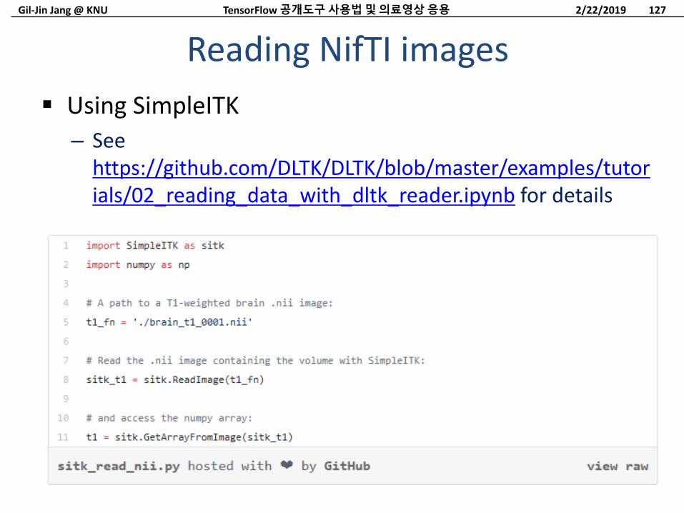
Using SimpleITK
– See https://github.com/DLTK/DLTK/blob/master/examples/tutorials/02_reading_data_with_dltk_reader.ipynb for details
Reading NifTI images
2/22/2019TensorFlow 공개도구사용법및의료영상응용 127
Gil-Jin Jang @ KNU
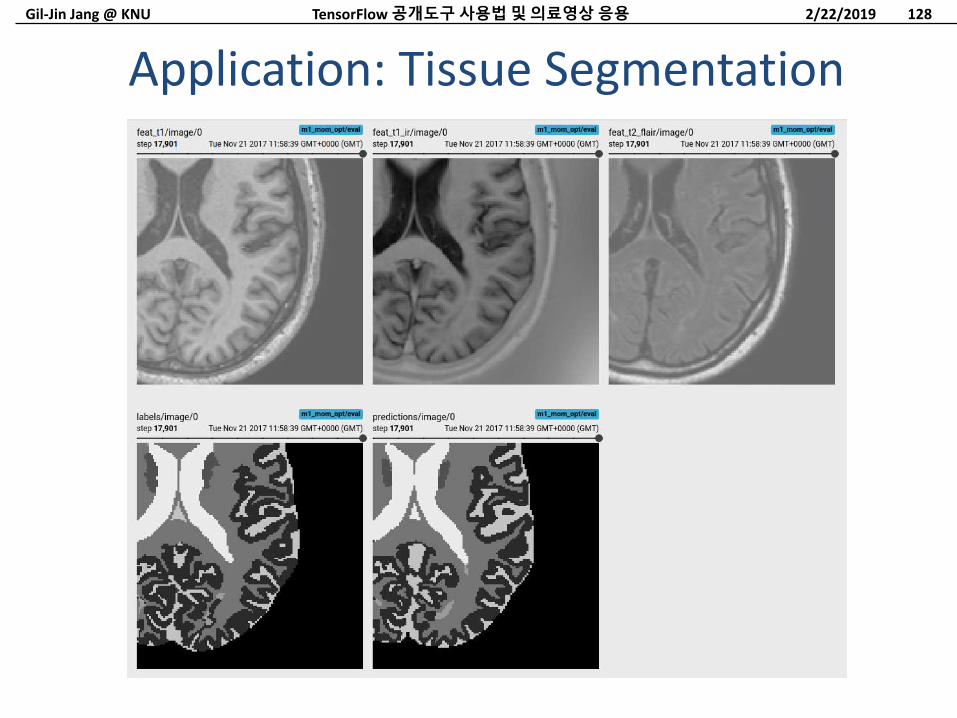
Application: Tissue Segmentation
2/22/2019TensorFlow 공개도구사용법및의료영상응용 128
Gil-Jin Jang @ KNU
Application: Tissue Segmentation
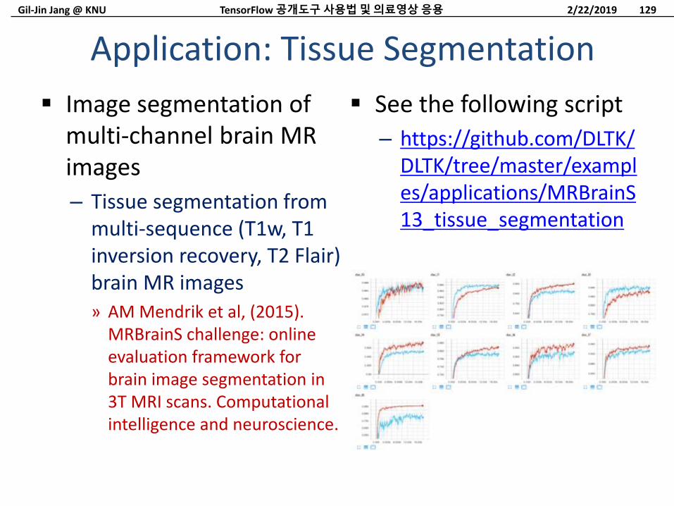
Image segmentation of multi-channel brain MR images
– Tissue segmentation from multi-sequence (T1w, T1 inversion recovery, T2 Flair) brain MR images» AM Mendrik et al, (2015).
MRBrainS challenge: online evaluation framework for brain image segmentation in 3T MRI scans. Computational intelligence and neuroscience.
2/22/2019TensorFlow 공개도구사용법및의료영상응용 129
See the following script
– https://github.com/DLTK/DLTK/tree/master/examples/applications/MRBrainS13_tissue_segmentation
Gil-Jin Jang @ KNU
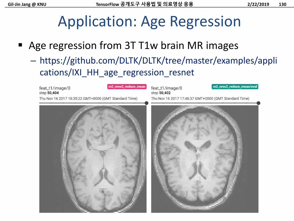
Age regression from 3T T1w brain MR images
– https://github.com/DLTK/DLTK/tree/master/examples/applications/IXI_HH_age_regression_resnet
Application: Age Regression
2/22/2019TensorFlow 공개도구사용법및의료영상응용 130
Gil-Jin Jang @ KNU
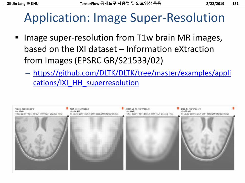
Image super-resolution from T1w brain MR images, based on the IXI dataset – Information eXtractionfrom Images (EPSRC GR/S21533/02)
– https://github.com/DLTK/DLTK/tree/master/examples/applications/IXI_HH_superresolution
Application: Image Super-Resolution
2/22/2019TensorFlow 공개도구사용법및의료영상응용 131
Gil-Jin Jang @ KNU
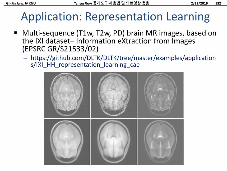
Multi-sequence (T1w, T2w, PD) brain MR images, based on the IXI dataset– Information eXtraction from Images (EPSRC GR/S21533/02)– https://github.com/DLTK/DLTK/tree/master/examples/application
s/IXI_HH_representation_learning_cae
Application: Representation Learning
2/22/2019TensorFlow 공개도구사용법및의료영상응용 132
Gil-Jin Jang @ KNU
U-NETEfficient Image Segmentation
2/22/2019TensorFlow 공개도구사용법및의료영상응용 133
Gil-Jin Jang @ KNU
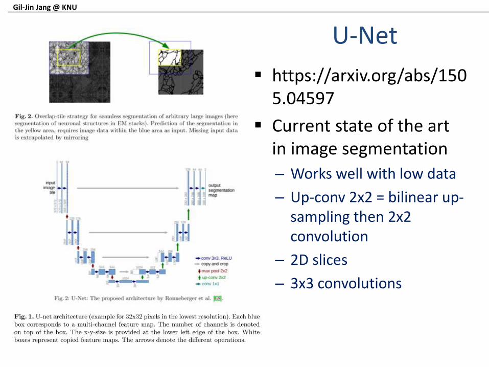
U-Net
https://arxiv.org/abs/1505.04597
Current state of the art in image segmentation
– Works well with low data
– Up-conv 2x2 = bilinear up-sampling then 2x2 convolution
– 2D slices
– 3x3 convolutions
Gil-Jin Jang @ KNU
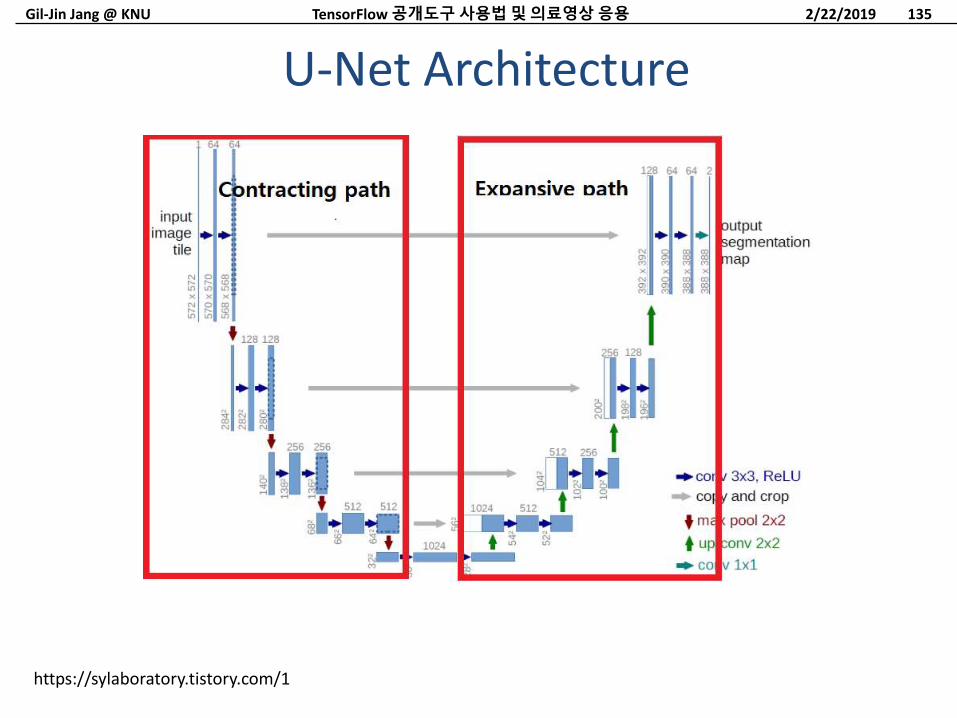
U-Net Architecture
2/22/2019TensorFlow 공개도구사용법및의료영상응용 135
https://sylaboratory.tistory.com/1
Gil-Jin Jang @ KNU
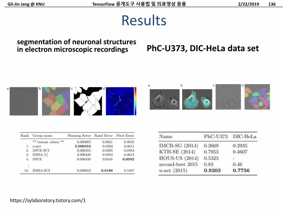
Resultssegmentation of neuronal structures in electron microscopic recordings PhC-U373, DIC-HeLa data set
2/22/2019TensorFlow 공개도구사용법및의료영상응용 136
https://sylaboratory.tistory.com/1
Gil-Jin Jang @ KNU
TensorFlow
– 다양한 open source recipe들이제공됨
Medical image analysis
– Successful results with tensorflow
ConclusionTensorFlow 공개도구사용법및의료영상응용 1372/22/2019