Embed Size (px)
Citation preview

Food Consumption Patterns, Seasonality, & Market Access in
Mozambique*
Sudhanshu Handa* Department of Public Policy University of North Carolina CB #3435 Chapel Hill, NC 27599-3435 [email protected]
Gilead Mlay Faculty of Agronomy Eduardo Mondlane University C.P. 257, Maputo Mozambique [email protected]
Abstract Seasonal fluctuations in food consumption is a serious problem in rural Mozambique where community isolation is high, and market integration, use of improved inputs, and access to off-farm income, is low. This paper uses household survey data to trace out the existence of seasonal fluctuations in food consumption patterns, and to analyze possible coping strategies employed by households to maintain access to calories. Significant substitution is observed between maize and cassava, and beans and green vegetables, over the production cycle. An analysis of the total expenditure elasticity of food groups reveals the precarious food security situation of rural households in the poorest quintile. These households show near unitary expenditure elasticity for even the most basic staples of cassava and maize. The potential role of public policy in diminishing seasonal fluctuation in food consumption is explored using distance to road as an indicator of market access. The results show that households within 4-5 kilometers of a road have significantly lower pro-cyclical fluctuation in food consumption patterns. * Corresponding author. Thanks to Emilio Tostao, Farizana Omar, Virgolinho Nhate, and Anibal Nhampossa, for excellent research assistance, and to David Tschirley for useful comments.

1
1. Introduction An important challenge in the quest for food security among poor agricultural
households is sustaining food consumption during the lean season. This is especially true
for farm households that rely on rain fed agriculture, and who have poor post-season
storage capacity, or limited market opportunities to monetize post harvest surpluses. A
number of studies have documented the extent of consumption seasonality in developing
countries, as well as the behavioral responses that agricultural households display in the
face of extreme fluctuations in income due to the agricultural cycle.1
This paper explores some of these issues using the first national household survey
of Mozambique, one of the poorest countries in the world, and where food security is a
primary concern. Over 80 percent of Mozambique’s 16 million people live in rural areas
and depend on agriculture for their survival, yet only 3 percent use improved agricultural
inputs, and a similar percentage use non-rain fed sources of irrigation. Given these
conditions, and the geographic isolation of rural communities, income seasonality and its
implications are important policy issues in the country.
Our analysis on this subject is divided into two parts. In the first part, we illustrate
the seasonal variability in food consumption patterns of households, relating these to the
agricultural production cycle as well as the typical diet in the country. Given this diet, we
show how households substitute among food groups in order to maintain a balanced diet,
and the key role that cassava plays in providing calories to households during the lean
season. We also provide estimates of income elasticities for staple and non-staple foods,
which demonstrate the precarious food security position of rural households, especially
those in the poorest quintile.
In the second part of the paper, we evaluate the extent to which market access affects
food consumption patterns as well as the variability of food consumption among rural
households over the agricultural cycle. We find distinct differences in the food
1 The collection of articles in Sahn (1989) provide an introduction and overview of the issue of seasonality and its consequences among agricultural households in developing countries. Other studies that evaluate the extent and consequences of seasonality can be found in Paxson (1992, 1993) and Alderman (1996).

2
consumption patterns of households that we classify as having more market access, and in
particular, find that these households display less fluctuation in the consumption of staple
foods. These results have important implications for public policies in the rural areas
whose objectives are to smooth consumption over the production cycle in order to reduce
the risk of food insecurity during the lean season in rural Mozambique.
2. The Setting
Since 1993, the economy of Mozambique has enjoyed high growth rates reflected by
average annual GDP growth of 7.9 % between 1993 and 1997. This turn around in economic
performance is attributed to the return of social and political stability following the
cessation of hostilities between RENAMO and the government in 1992 and subsequent
democratic multiparty elections in 1994, the on-going institutional and economic reforms
initiated in 1987 and favorable weather conditions leading to a significant increase in
agricultural production.
The return of stability has led to the resettlement of the majority of people displaced
by war and the re-initiation of normal agricultural activities. The quick agricultural
recovery is witnessed by the decline of maize imports in the form of food aid from 563000
metric tons in 1992 to 14000 metric tons in 1996, and the reduction of the number of people
depending on food aid, which declined from 3.8 million to 154000 in the same period
(MAP, 1997)
Although there are significant visible signs of economic recovery, it is not clear to
what extent this has translated into the improvement of the well being of disadvantaged
groups in the society. Mozambique’s GDP per capita is still one of the lowest in the
world, and it is estimated that more than 60% of the urban population and 70% of the rural
population live in absolute poverty. It is also estimated that 43% of preschool children
suffer from long term malnutrition (height for age z-score less than or equal to –2) and
22% suffer from acute malnutrition (height for age z-score less than or equal to –3) (MPF,
1998).
The government of Mozambique is taking short and long term measures geared

3
towards reducing poverty and food insecurity. A national agrarian policy and strategy for
implementation was approved in 1995. The document charts out the agrarian development
objectives and defines the strategies to attain them in the medium and long term. On the
basis of the national agrarian policy, a national program for agrarian development
(PROAGRI) was prepared and was approved in 1998 (MAP, 1998) while a national strategy
for food security and nutrition has also been approved by the Council of Ministers. This
latter strategy aims at achieving food security mainly through market mechanism in which
the government plays a facilitating role. The document recognizes the need to continue
with targeted programs for the disadvantaged groups in the society.
3. The Data and Descriptive Statistics
For purposes of planning and monitoring policy impact on household food security
and nutrition, an understanding of household food consumption patterns and forces
causing changes in these patterns is a necessity. Given data limitations imposed by
Mozambique’s violent history, there have only been a few previous studies that looks at
food consumption patterns and behavior in Mozambique and these focus on specific
geographical areas, usually specific provinces in the rural north or Maputo city [Dengo
(1992); Rose et.al (1998); Sahn & Desai (1995); Tschirley & Santos (1994)].
In 1996/97 a national household survey of Mozambique was conducted by the
National Statistical Institute. This survey, called the Inquerito Nacional Aos Agregados
Familiares (IAF) is nationally representative, and was carried out over a 14 month period
beginning in February 1996. The survey design was a 3-stage stratified random sample,
with rural-urban designating the strata, and the administrative unit known as the locality
defining the primary sampling unit.2 We exploit the fact that the IAF was carried out
over an entire year to identify seasonality effects in consumption. Table A1 in the
appendix shows the number of households in each region that were interviewed in each
2 Our estimates of standard errors take into account correlations due to sampling design, and summary
descriptive statistics are population weighted in order to be representative of the country.

4
month of the year (total sample size is 8250 households). In the rural region the
distribution of households over the 12 months is quite good, which helps us in identifying
seasonal affects over this cross-section. In urban areas however, most households were
interviewed at the beginning of the year, so that the representation of households is small
between August and November. This means that our estimates of seasonality will be
poorly measured for these months, which should be kept in mind in the proceeding
analysis. Because of this potential weakness of the data, we concentrate most of our
discussion around rural households, and also group households into 3 time periods in
order to have enough observations within each period with which to make meaningful
inferences.
In terms of information, the IAF is a standard multi-purpose household survey, with
an extensive consumption expenditure module, as well as modules on health, education,
agricultural production, and migration. Total household welfare is measured by total
household expenditure on consumption per capita, and this is normalized by a regional
and seasonal price index in order to be comparable across households from different
regions and interview months.3 Our analysis of consumption patterns is based on budget
shares so that we avoid the problem of regional cost of living differences.
In Tables 1 and 2 we provide some descriptive information on the degree and type
of consumption seasonality found in Mozambique. In Table 1 we present the results of
simple OLS regressions that relate total consumption, total food consumption, and the
food share, to a set of monthly and provincial dummy variables. Wald tests for the joint
significance of the monthly dummy variables, shown at the bottom of the table, give us an
idea of the importance of consumption fluctuations over the year among these households.
In only one case are these monthly dummies not significant as a whole, and that is for total
consumption in rural areas. This is probably because overall mean consumption is so low
3 Technical details of the construction of the consumption aggregates and price indexes can be found in MPF, 1998.

5
in rural Mozambique to begin with.4
Table 2 presents mean shares out of total food consumption for the two basic staples
of cereals and roots and tubers, as well as the most important sub-group within these two
(maize and cassava). In Mozambique, as in most of southern Africa, the basic staple is
maize, and the harvest season for maize begins in March and can go up to May depending
on how far north one is. Similarly, the sowing period begins in September and can last
until November in some parts of the country. Hence the last trimester of the year
(September through December) is the lean season, when stocks from the previous harvest
begin to run low, and the end of the first trimester (January through April) and the second
trimester are ‘peak’ seasons, when stocks of maize are high and food insecurity low. 5 The
behavior of the maize share follows this cycle very closely. In rural areas, the share of
maize is lowest during the lean season (0.198 in September – December), and increases
steadily in trimester 1 and 2. The behavior of the cassava share is exactly opposite to this,
as cassava is the ‘food security’ crop in this region of Africa, and is consumed in the lean
season as a substitute for maize. The share of cassava in the food budget is highest in the
lean season (trimester 3), and then declines steadily until it reaches a low of 0.114 in the
second semester, when the maize share is highest.
In urban areas the pattern is slightly different due to the importance of bread and
wheat based products in the diet. For example, while the share of maize is lowest in the
lean season, the total cereal share actually rises to 0.400 in trimester 3, primarily due to the
importance of imported wheat and wheat based products in the diet. The overall food
share actually fluctuates very little over these three trimesters in urban areas, while in rural
areas there is a significant jump in the food share in the hungry season, from 0.679 in
trimester 2 to 0.702 in trimester 3.
4 Mean per capita daily consumption is 50 U.S. cents per day in rural areas. 5 This is a general characterization that we make for analytical convenience and is meant to represent the
average trend in the country; in specific areas, January and even some of February can be the tail end of the lean
season.

6
We complete our descriptive analysis by presenting estimates of total expenditure
elasticities for food over the year. These are estimated by regressing log total expenditure
on the log of total food expenditure, with seasonal differences calculated by allowing for
dummy interactions between each of the 11 monthly dummies and the log total
expenditure variable. These interaction terms are jointly significant, and the calculated
elasticities are shown in the appendix Table A2. The elasticity pattern is shown in Figure 1
for urban and rural regions separately. Urban areas are richer than rural ones in
Mozambique, and the estimated food elasticities are accordingly lower in urban relative to
rural areas. However, these elasticities come together at the height of the lean season
(December and January). The rural food elasticities are very high, reaching 1 in March,
indicating that virtually all additional income during this period is devoted to food
purchases.
3. Methodology
Our principal analytical tool is the Engel curve, which relates budget shares
devoted to various food groups, to total household expenditures and other household
characteristics such as demographic composition. The exact specification we use is what is
now commonly known as the Working-Leser functional form, for which applications can
be found in Deaton & Muellbauer (1980) and Handa (1996), among others. This
specification looks like the following:
(1) ( ) ( ) i5432
21 log log εβββββαω +∗+∗+∗+∗+∗+= SeasonDemoXconconi
where wi is the budget share for commodity i, con is household total per capita
consumption expenditures, X is a vector of household characteristics, Demo are a set of
demographic variables measuring the number of people in 6 age groups, Season are a set of
dummy variables indicating the time period in which the household was interviewed,
alpha and the betas are parameters to be estimated, and ε i is a random error term. The

7
control variables included in the X vector include the following: total land holding,
whether the household uses any modern agricultural inputs (irrigation, fertilizer, or
equipment), age, sex, and education of the household head, and the year of the interview
(1996 or 1997). Seasonality is captured by month of interview, and is sometimes
aggregated to trimesters (i.e. 4 month periods) and sometimes monthly.
Using equation (1), the marginal effect on the budget share of a change in total
household expenditure is given by (2), while the total expenditure elasticities can be
derived using the formula in (3) (Deaton et.al. 1989):
(2) Mw i/M(log(con))= β1+2*β2* log(con)
(3) ( )[ ] ( )[ ] iii conconE ωββωω /log2 1 /log/ 1 21i ∗++=∂∂+=
Most of the analysis on seasonality is carried out using budget shares out of total food
expenditures on the left hand side of equation (1). However the elasticity calculation set
out in equation (3) is based on the budget share out of total expenditure, and so for our
estimates of elasticities we use this as our dependent variable. As mentioned earlier, all
standard errors are corrected for the sample design effects of the IAF.
4. Results on Seasonality, Consumption Switching, and Elasticities
a) Seasonality effects and consumption switching
Vegetables, beans, meats and fish are normally eaten together with a cereal (maize,
rice and wheat derived products) or starchy (cassava, sweet potatoes, Irish potatoes) main
dish. It is therefore reasonable to assume that vegetables, beans, meats and fish are
substitute products, and likewise cereals are substitutes for starchy foods and vice versa.
The fact that production is seasonal, availability (supply) along the year will also influence
consumption pattern over a year. This will be more pronounced in the presence of market
failure. Perishable seasonal products like vegetables are expected to show higher seasonal
fluctuations than cereals. Noting that rural household expenditure on food is largely based

8
on subsistence production, local climatic conditions which influence production
possibility over a year will have a great bearing on the nature of seasonal effects on food
consumption patterns. In addition, the cash income of such households is also seasonal
since it is mainly derived from sales of surplus production.
We estimate equation (1) by region on 8 broad food groups: cereals, roots and
tubers, meats, seafood, legumes, fruits, green vegetables, and other foods. We capture
seasonality using monthly dummy variables (December is the excluded category), and
results for these seasonality effects for cereals and roots and tubers are presented in Table
3. The Wald test for joint significance of the seasonal variables is significant in all cases
except for cereals in rural areas. Figures 2 and 3 graph the predicted budget shares based
on the regression coefficients for rural and urban areas respectively. In Figure 2 (rural), the
cereal food share is highest in the first 2 trimesters and lowest in the last trimester (with the
exception of January), while for roots and tubers the seasonality effect is exactly the
opposite, as we would effect, with the share highest during the lean months in the last
trimester of the year, and lowest in the other periods. Note that the curves almost always
move in opposite directions, the budget share for tubers declining when that for cereals
increases, and vice versa. This behavior clearly indicates the substitution that takes place
between these two food groups among Mozambican households.
Among urban households (Figure 3), the overall share of cereals is much higher,
and that of tubers lower, than in rural areas, but the same general picture of substitution
between these two groups is revealed. The estimated share of cereal is highest in trimester
3, exactly when the estimated share of roots and tubers is lowest. Furthermore, the same
‘mirror’ image exists in the pattern of expenditures among urban households—the share of
roots and tubers in the budget almost always moving in the opposite direction as the share
of cereal.
In Tables 4 and 5 we present the seasonality effects for the 6 other food groups that
we consider. In rural areas, 5 of the 6 food groups display significant seasonality over the
year (see joint test of significance at the bottom of Table 4), with seafood being the only

9
exception. In urban areas (Table 5), 4 of the 6 food groups display significant fluctuations
over the year, the exceptions here being green vegetables and other foods.6 The degree of
seasonal fluctuation among urban areas is surprising given that incomes tend to be more
stable and imported foods are available in the large urban centers in the south of the
country (Maputo City, Matola, and Xai-Xai).
In light of our description of the typical Mozambican diet, we expect vegetables and
beans to be substitutes in their role as accompaniments to maize (xima) or cassava, and so
we evaluate this hypothesis in Figures 4 and 5, which graph the month coefficients
presented in Tables 4 and 5. For rural areas (Figure 4), the substitution between these two
groups is quite evident, with the green vegetable share highest at the beginning of the year
and lowest at the end of the year, and vice versa for legumes. In urban areas (Figure 5) the
annual fluctuation is relatively smaller (recall that for vegetables the joint effects are not
significant), but the basic pattern seems to be the same, with the legume share lowest at the
beginning of the year and rising at the end of the year.
b) Total expenditure elasticities
We calculate and present total expenditure elasticities by food group in Table 6, for
rural and urban areas, and separately by consumption quintile. Elasticities above 1 are
usually considered luxuries, and those below 1 necessities. Using the magnitude of the
elasticities as a measure of the degree of necessity, the degree of necessity for all rural
households increases in the following order: maize (0.994), roots and tubers (0.833), green
vegetables (0.827), cassava (0.817), and beans (0.656). Meats, other foods, and seafood are
estimated to be luxuries. Elasticities tend to be higher for households in the bottom
quintile, although beans (legumes) is an exception, probably because these are more likely
to be consumed out of home production for poor households. The striking thing is that for
poor rural households, cereals and maize have elasticities well over 1, indicating that these
staples are still luxuries for the very poorest in rural areas. Even roots and tubers and
cassava, which tend to be stored in the ground and used as crop insurance, have
6 Full results from the Engel curve regression estimates are presented in the appendix.

10
elasticities close to 1. Taken together these results demonstrate the extremely precarious
food security situation faced by poor rural households in Mozambique.
Urban expenditure elasticities tend to be lower than rural ones, and for the sample
as a whole, only two commodity groups are estimated to be luxuries (meats and other
foods). The elasticities for staple foods such as cereals and roots and tubers are well below
1, and are even lower among the richest quintile. Among the poorest urban quintile, meats
and other foods are also clear luxuries, while roots and tubers and seafood have unitary
elasticities.
Given that household food expenditure is largely based on subsistence production
in rural areas, and that rural households are in general poorer than urban households,
large differences are expected between urban and rural households in the degree of
responsiveness of food consumption patterns to total expenditure. And while rural
elasticities do tend to be higher than urban ones, one important exception is meats, where
urban elasticities are higher than rural ones for all quintiles shown. This is due to the fact
that rural meat consumption is essentially based on home production (including hunting),
while urban households depend on market purchases for their meat.
In Mozambique, market access and integration and well-being tends to increase
from North to South7, so in Table 7 we present total expenditure elasticities by region to
see if these regional characteristics result in different responses to changes in total
expenditure or income. Given these characteristics, we would expect elasticities to be
higher in the north relative to the south, although the degree of variation across zones
might be smaller in rural relative to urban areas. In fact the elasticity estimates presented
in Table 7 display this pattern with surprising consistency although a few exceptions exist.
In the rural region, there is very little variation in estimated elasticities as we move from
north to south, and in some cases (total food, cereals, meats, and vegetables) the estimated
7 As with the description of the harvest and lean seasons, the characterization of market access and integration as decreasing from south to north is simplistic. The border areas in the rural north engage in trade with Malawi and Nampula is densely populated with a major international port. On the other hand parts of western Gaza in the south can be quite isolated.

11
elasticities are actually slightly higher in the south, again due to the fact that households in
the north are more likely to consume these products out of home production.
In the urban areas on the other hand, elasticities tend to decline as we move from
north to south, especially for the basic staples like maize and cassava. Overall food
elasticities (the first line in Table 7) also decline significantly as we move from northern to
southern Mozambique. Hence, it appears that market integration both in terms of access to
imported foods as well as access to more stable sources of income, can have an important
affect on food consumption patterns, and ultimately on food security, in Mozambique. We
now provide a more detailed analysis of this hypothesis in the next section.
5. Market Access and Consumption Seasonality
a) Regional differences in seasonality among rural households
The analysis above reveals that rural households face larger fluctuations in food
consumption, and there is significant variation in household response to income changes
as we move from the more isolated north to the more integrated south of Mozambique.
We quantify this variation more rigorously by focussing on rural households only, and
estimating separate Engel curves for the north, center, and south of the country. Due to
sample size issues, we cannot include the full 11 monthly dummy variables, but rather
capture seasonality by grouping interview date into three groups: trimester 1 (January –
April), trimester 2 (May – August), and trimester 3 (September – December). We use
trimester 1 as the excluded category, and expect that seasonality in food budget shares will
be strongest in the north, which is most isolated, and diminish as we move towards the
more integrated southern part of the country.
Table 8 reports p-values for the joint test of significance of the two seasonal dummy
variables for each Engel curve regession, by region. Seasonality is very significant in the
north, where 9 of the 10 food groups display significant fluctuations over the three
trimesters. Moreover, these seasonal fluctuations are less evident in the central and
southern rural regions, although in each of these two cases, 4 of the 10 commodity groups
display significant seasonal variation at the 10 percent level.

12
To assess the pattern and degree of consumption switching, we present the actual
coefficient estimates (and t-statistics) for the two seasonal dummy variables for the staple
foods of maize and cassava (Table 9), and for the broad groups of cereal and roots and
tubers (Table 10). Recall that the beginning of the harvest season is the excluded group,
when maize consumption is high, so we expect the coefficients for maize (and cereal) to be
negative, and the coefficients for cassava (and roots and tubers) to be positive.
The results of the joint test for seasonality in Table 10 indicate that seasonality
declines as we move from north to south. The coefficients on the trimester dummy
variables are largest and statistically significant in the north , and decline in (absolute)
value and in significance as we go south. When we analyze the specific commodities of
maize and cassava in Table 9, we also find that seasonality effects are strongest in the
northern part of the country. The other interesting thing to note is the almost perfect
substitution between cereals and tubers (or maize and cassava) during trimester 3 (the lean
season). For example, the point estimates in Table 10 indicate that in trimester 3 in the
north, the cereal food share declines by .10 percentage points while that of tubers increases
by .14 percentage points. In the central region the substitution is perfect: a .06 percentage
point decline in cereals in trimester 3 is exactly offset by a .06 percentage point increase in
tubers in the same period. This strong substitution is clearly an important mechanism
employed by households to reduce the risk of food insecurity over the production cycle in
rural Mozambique.
b) Market access and seasonality in Northern Mozambique
In this section we investigate the role that market access can play in seasonality in
food consumption, and by doing so, seek to highlight the potential role for public policy in
reducing food insecurity in the country.
We have available to us the distance to the nearest road for each village in the IAF
sample. This information was calculated by Geographical Informations Systems based on
geographical information provided by the Mozambican Directorate of Geography and
Cadasters (DINAGECA), and details of these calculations are provided in Nhate (1999).

13
We use distance to nearest road as a rough indicator of access to markets and alternative
sources of income, and hypothesize that increased market access may allow households to
smooth consumption over the agricultural production cycle. We experimented with
several different approaches to measure the effect of distance to road on food consumption
patterns, including separate sample estimates and interaction terms. While interactions
(between distance and the trimester dummies) allow for formal hypothesis tests, we end
up with an enormous quantity of regression coefficients that are cumbersome to interpret.
We therefore take a simpler approach and estimate a series of Engel curves on households
located at different distances from a road. We estimate these regressions on 6 budget
shares (maize, cassava, cereals, tubers, legumes, and vegetables) for all rural households,
for 10 different distances, and focus on the difference in the budget share between trimester
1 (the excluded group) and trimester 3 (the lean season).
We also have direct evidence of alternative sources of income through the IAF
employment module. Using that information we construct a dummy variable indicating
whether the household has any off-farm sources of income. However unlike distance to
road, this information on income source is endogenous to household decisions on food
consumption, a problem that would normally require instrumental variables to correct.
Nevertheless, we provide some provisional estimates of the association between the
presence of an off-farm income source and fluctuations in food consumption patterns,
hypothesizing that these sources of income will serve to dampen the seasonal fluctuation
in food consumption, although the precise cause and effect mechanism still remains to be
clarified.
Distance to road: Table A5 in the appendix summarizes the coefficient estimates for the
dummy variable indicating trimester 3, for 10 different sub-groups of households, for the 6
commodities mentioned above. The distances we consider are: 0-2 kilometers from a road,
and then greater than 2, 3, 5, 6, 8, 12, 16, 20, and 24 kilometers from the nearest road.
Sample sizes for each of these sub-groups are also presented in Table A5.
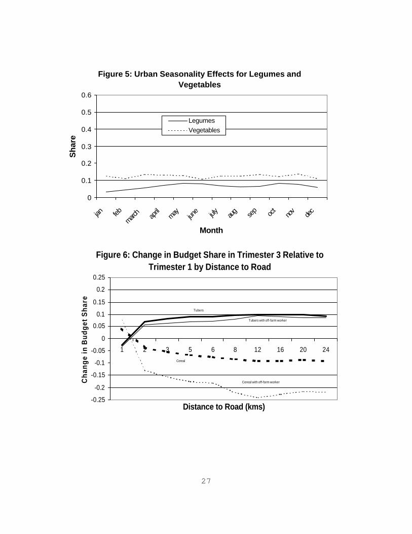
The easiest way to assess the relationship between market access and seasonality is

14
graphically, so we graph the point estimates for trimester three for each distance in Figures
6, 7, and 8. Figure 6 presents this relationship for the broad groups of cereals and tubers,
and the results are startling. Both commodities display counter-cyclical patterns for
households that live within 2 kilometers of a road—the trimester 3 coefficient is positive
for cereal and negative for tubers. However, for households living over 2 kilometers from
a road, there seems to be a strong positive relationship between fluctuation in the trimester
3 budget share and distance to a road. In the case of cereals, this relationship becomes flat
after approximately 10 kilometers, while for tubers the relationship flattens out sooner—at
approximately 6 kilometers.
Figure 7 displays this relationship for maize and cassava budget shares, and the
same general patterns emerges. Households within 2 kilometers of a road display
counter-cyclical consumption of these commodities, while households over 2 kilometers
from a road display the usual pattern of reduced maize offset by increased cassava during
the lean season. Note that the curves flatten out sooner than in Figure 6--at around 5-6
kilometers in both cases.
Figure 8 graphs the coefficients for legumes and vegetables, and here we see a
weaker relationship between market access and fluctuations in trimester 3 budget shares
relative to trimester 1. In both cases, there is a small initial jump between 0-2 kilometers
and greater than 2 kilometers, but then the curves essentially flatten out, indicating that
there is no further ‘penalty’ in terms of fluctuations in the budget share after 2 kilometers.
Off-farm sources of income: We repeated the regressions described above on the sub-
sample of households who indicated they had an off-farm source of income, to see whether
this select group of households displays less seasonal fluctuation in consumption over the
year. In a similar manner as before, we graph the trimester 3 dummy variable for different
groups of households based on their distance to a road, and expect to see a weaker
relationship between distance and this coefficient than we observed over the full sample.
For ease of comparison, these coefficients are also graphed in Figures 6-8.
The results for tubers (Figure 6) and cassava (Figure 7) are as we expected. The sub-

15
sample of households with an off-farm worker display less fluctuation in their trimester 3
consumption of these two commodities relative to the full sample (the lines for this group
are closer to the x-axis relative to the line representing the full sample). However the
opposite is found for the cereal and maize consumption. In this latter case, the sub-sample
of households with an off-farm worker actually display more fluctuation in trimester 3
relative to the sample as a whole (the line representing off-farm households lies outside
the line representing the full sample for these two commodities). Indeed the differences in
the trimester 3 coefficients are quite large. In the case of maize, for households 8 or more
kilometers from a road, the difference in the food budget shares is 0.10 percentage points!
We see from Figure 8 that this difference in cereal (and maize) consumption is
entirely explained by different behavior towards the consumption of green vegetables in
trimester 3 by households with an off-farm worker. For these households, the budget share
for green vegetables is nearly .10 percentage points greater than the full sample, for
households living over 8 kilometers from a road. These results probably reflect the fact
that off-farm employment and food consumption patterns are simultaneously determined.
For example, rural households may be sacrificing own farm maize production in exchange
for off-farm sources of cash income, and using this income to compensate for maize
shortages in the lean season through purchases of green vegetables (which are available at
that time). Note however, that households with off-farm income have less trimester 3
fluctuations in the budget share of legumes. A complete analysis of the full set of Engel
curves for these households also indicates slightly higher consumption of meat during the
lean season, relative to the full-sample, which offsets the lower consumption of beans
observed in Figure 8 (results available upon request).
6. Conclusions and Policy Implications
Our analysis of the food consumption behavior of Mozambican households reveals
some important patterns which can inform the country’s food security strategy. Perhaps
the most important initial observation is the high (nearly unitary) income elasticity for
basic staple foods among poor (bottom quintile) rural households. For these households,

16
even the most basic products such as cassava have unitary income elasticity, verifying
what development agencies and government officials have also recognized, which is that
the food security situation of this group is precarious.
Consistent with the low use of agricultural technology and market access, seasonal
fluctuations in consumption are important, and closely follow the agricultural production
cycle. Our analysis shows clear compensatory behavior by households in an effort to
equalize the consumption of calories over the production cycle, through increased
consumption of cassava and other roots and tubers during the lean season when maize
stocks are low. Significant substitution along the production cycle is also observed
between legumes and vegetables, both important components in the typical diet,
especially in the rural regions.
The Government of Mozambique has committed itself to a market based
development strategy, and the results in this paper show that increased market integration
can lead to benefits in terms of reduced fluctuations in consumption over the agricultural
season. First, seasonal fluctuation in the consumption of different food groups is
significantly higher in the more isolated northern region than in the more integrated center
or south. Second, among rural households, access to markets, measured by distance to the
nearest road, is strongly associated with reductions in pro-cyclical fluctuations in food
consumption. For example, in the case of maize, households that live over 8 kilometers
from a road suffer a reduction in maize share in the lean season of almost 10 percentage
points, compared to 5 percentage points for households that live 2 kilometers from a road.
And households that live less than 2 kilometers from a road actually display counter-
cyclical fluctuation in maize share. Similarly, households at 10 or more kilometers from a
road display pro-cyclical fluctuations in their cassava food share of 7 percentage points,
while those living within 2 kilometers of a road display counter-cyclical fluctuations in
their cassava food share. These results indicate that infrastructure development projects
aimed at increasing market access and integration for isolated rural households can have
an important impact in reducing seasonal fluctuation in food consumption patterns in

17
these areas.
Finally, we provide some tentative results on the association between the existence
of off-farm sources of income for the household, and seasonal fluctuation in food
consumption patterns. We find that seasonal fluctuation in consumption behavior is
conditioned by the presence of an off-farm source of income in the household. In the case
of basic foods such as cassava, vegetables, and beans, households with off-farm
employment display less seasonal variation in consumption over the year, compared to
those without an off-farm income source. In the case of maize, however, this group of
households actually displays greater pro-cyclical consumption variation, which is
supported by greater consumption of vegetables and meats during the lean season. This
suggests that the overall diet of those households with an off-farm source of employment
may be more balanced, but the cause and effect relationship between these two variables
still requires further analysis.
References Alderman, Harold, 1996, “Saving and Economic Shocks,” Journal of Development Economics, 51(2), 343-365. Dengo, M.N.C. (1992), Household Expenditure Behavior and Consumption Growth Linkages in Rural Nampula Province, Unpublished M.Sc. Thesis, Michigan State University. Deaton, A., Case, A. (1993), Analysis of Household Expenditure, LSMS Working Paper No. 28, The World Bank, Washington, DC. Deaton, Angus, and John Muellbauer, 1980, Economics and Consumer Behavior, New York, Cambridge University Press. Deaton A., Ruiz J.C, Thomas, D (1989), “The Influence of Household Composition on Household Expenditure Patterns: Theory and Spanish Evidence,” Journal of Political Economy, 97, 179-120

18
Handa, S. (1996), “Expenditure Behavior and Children's Welfare: An Analysis of Female Headed Households in Jamaica,” Journal of Development Economics; 50, 165-187. Ministerio de Agricultura e Pescas, (1998), Programa Nacional de Desenvolvimento Agrario (PROAGRI): 1998- 2003, Maputo, Mozambique. Ministerio de Agricultura e Pescas, (1995), Politica Agraria e Estrategias de Implementacao, Direccao de Agricultura, Maputo, Mozambique. Nhate, V. (1999), Infraestructura, Bem-Estar Familiar e Pobreza em la Zona Rural em Moçambique, Trabalho de Diploma, Faculty of Agriculture and Forestry Engineering, Eduardo Mondlane University, Maputo, Mozambique. C. Paxson, 1992, “Using weather variability to estimate the response of savings to transitory income in Thailand,” American Economic Review, 82, 15-33. C. Paxson, 1993, “Consumption and Income Seasonality in Thailand,” Journal of Political Economy, 101, 39-72. Rose, David, P. Strasberg, J. Jeje & D. Tschirley, 1998, “Household Food Consumption in Mozambique: A Acse Study in Three Northern Districts,” Research Report 33, Ministry of Agriculture, Government of Mozambique. Sahn, David (ed), 1989, Seasonal Variation in Third World Agriculture: The Consequences for Food Security, Baltimore, Md., Johns Hopkins University Press for the International Food Policy Research Institute. Sahn D. & J. Desai, 1995, “The Emergence of Parallel Markets in a Transition Economy: The Case of Mozambique,” Food Policy 20(2): 83-98. Tschirley, D. & A.P. Santos, 1994, “Who Eats Yellow Maize: Results of a Survey of maize Meal Preferences in Maputo,” Research Report 18, Ministry of Agriculture, Government of Mozambique.

19
Table 1: OLS coefficient estimates of monthly dummy variables by region
(Only provincial dummies included as controls) RURAL URBAN
Dep. Variable: log consumption log total food food share log consumption log total food food share
January -0.020 -0.093 -0.018 -0.082 -0.072 0.023 February -0.126 -0.201 -0.014 0.098 -0.075 -0.051 March -0.121 -0.184 0.007 0.073 -0.156 -0.053 April -0.173 -0.305 -0.005 -0.101 -0.259 -0.006 May -0.036 -0.048 0.009 0.104 0.033 -0.033 June -0.078 -0.146 -0.015 -0.009 -0.005 0.014 July -0.201 -0.303 -0.038 0.203 0.092 -0.042 August -0.134 -0.202 -0.025 0.514 0.350 -0.054 September -0.049 -0.118 -0.026 -0.290 -0.291 -0.014 October -0.090 -0.079 0.017 -0.387 -0.457 -0.039 November -0.002 0.012 0.019 -0.074 -0.060 0.006 December (constant) 11.862 11.641 0.592 12.389 12.269 0.570 F-test for months 1.45 2.72 1.91 4.05 4.37 3.45 p-value (0.15) (0.00) (0.04) (0.00) (0.00) (0.00) Observations 5811 2439 OLS regression estimates of the dependent variable named at the top of the column. Provincial dummy variables included in the regression but not reported. Coefficients with statistically significant (at 5 percent) t-statistics in bold. Table 2: Staple Food and Total Food Shares by Season (Means) Rural Urban Jan-April May-Aug Sep-Dec Jan-April May-Aug Sep-Dec Cereal 0.334 0.331 0.274 0.392 0.328 0.400 Maize only 0.233 0.252 0.198 0.215 0.155 0.110 Roots & Tubers 0.136 0.141 0.199 0.063 0.107 0.052 Cassava only 0.126 0.114 0.171 0.042 0.088 0.040 Food share 0.689 0.679 0.702 0.602 0.603 0.590

20
Table 3: Seasonality Effects on Budget Share of Cereals and Tubers by Region Rural Urban (1) (2) (3) (4) Cereals Roots and Tubers Cereals Roots and Tubers January -0.044 -0.023 -0.010 0.012 (0.71) (0.62) (0.23) (0.27) February 0.026 -0.079 0.041 -0.025 (0.40) (2.45) (1.14) (0.61) March 0.000 -0.022 0.003 -0.027 (0.00) (0.65) (0.09) (0.68) April 0.033 -0.067 -0.005 -0.045 (0.93) (2.67) (0.14) (1.13) May 0.024 -0.050 -0.013 -0.025 (0.66) (2.19) (0.35) (0.54) June 0.019 -0.019 -0.016 0.001 (0.47) (0.67) (0.44) (0.03) July 0.030 -0.054 0.023 -0.035 (0.74) (2.11) (0.64) (0.84) August 0.021 -0.028 -0.009 -0.008 (0.38) (0.69) (0.29) (0.22) September -0.018 -0.019 0.054 -0.037 (0.55) (0.79) (1.44) (1.05) October -0.006 0.013 0.073 -0.041 (0.17) (0.53) (2.42) (1.16) November -0.008 0.034 0.031 -0.035 (0.20) (1.21) (0.99) (0.99) Constant -3.860 -0.666 -2.167 0.558 (4.27) (1.77) (3.58) (1.56) R-Squared 13.71 21.02 13.29 18.55 F(months) 0.77 3.56 7.48 2.54 p-value for joint F-test 0.67 0.00 0.00 0.00 Observations 5811 2439 OLS coefficient estimates of Model 1. Absolute value of z-statistics in parentheses. Results for other variables included in the regression shown in the appendix.

21
Table 4: Seasonality Effects on Budget Shares of Food Groups -Rural (1) (2) (3) (4) (5) (6) Meats Fish & Seafood Legumes Fruits Green Vegetables Other Foods January -0.033 -0.017 -0.029 0.018 0.064 0.065 (1.90) (0.61) (1.60) (0.77) (1.47) (3.12) February -0.045 -0.017 -0.022 -0.044 0.119 0.062 (2.87) (0.61) (1.44) (2.67) (2.47) (3.31) March -0.058 -0.016 -0.024 -0.040 0.111 0.048 (3.97) (0.62) (1.55) (2.41) (2.60) (2.13) April -0.045 -0.008 -0.017 -0.036 0.090 0.051 (4.51) (0.39) (1.41) (2.73) (3.08) (3.42) May -0.039 -0.012 0.005 -0.048 0.091 0.028 (4.37) (0.37) (0.30) (3.35) (3.51) (2.58) June 0.000 0.019 0.007 -0.026 -0.022 0.023 (0.02) (0.64) (0.51) (1.40) (1.11) (1.82) July 0.002 -0.032 0.025 -0.039 0.047 0.021 (0.23) (1.18) (1.93) (2.61) (2.37) (1.49) August -0.007 -0.025 0.017 -0.034 0.037 0.020 (0.40) (1.08) (1.07) (2.06) (1.51) (1.44) September 0.019 -0.020 0.035 -0.034 0.018 0.019 (1.18) (0.82) (2.41) (2.30) (0.85) (1.91) October -0.015 -0.026 0.038 -0.028 0.013 0.010 (1.37) (1.20) (2.13) (2.01) (0.64) (0.90) November 0.002 -0.025 0.020 -0.021 -0.005 0.003 (0.13) (1.07) (1.44) (1.40) (0.21) (0.30) Constant -0.286 0.526 2.127 0.007 2.050 0.367 (5.77) (0.98) (3.55) (0.16) (3.22) (0.83) R-Squared 10.91 14.19 13.63 27.39 18.76 12.27 F(months) 5.73 0.58 3.21 2.16 4.00 2.06 p-value for joint F-test 0.00 0.85 0.00 0.02 0.00 0.02 OLS coefficient estimates of model 1, with absolute t-values given in parenthesis. Other results shown in the appendix. 5811 observations.

22
Table 5: Seasonality Effects on Budget Shares of Food Groups -Urban (1) (2) (3) (4) (5) (6) Meats Fish & Seafood Legumes Fruits Green Vegetables Other Foods January 0.000 -0.003 -0.017 -0.009 0.018 0.016 (0.01) (0.16) (1.36) (0.68) (0.92) (0.80) February -0.029 0.042 -0.016 -0.006 0.000 -0.002 (1.28) (3.12) (1.40) (0.52) (0.03) (0.12) March -0.020 0.027 0.000 -0.004 0.026 0.001 (0.92) (3.04) (0.05) (0.40) (1.77) (0.06) April -0.010 0.036 0.013 -0.011 0.017 0.010 (0.44) (3.56) (2.03) (1.10) (1.18) (0.63) May -0.037 0.034 0.022 -0.002 0.027 0.000 (1.60) (3.27) (3.08) (0.19) (1.96) (0.03) June -0.019 0.024 0.026 -0.005 0.001 -0.011 (0.86) (2.16) (3.22) (0.47) (0.07) (0.70) July -0.015 0.011 0.017 -0.010 0.015 -0.004 (0.64) (1.30) (2.42) (0.98) (1.32) (0.21) August -0.011 0.034 0.007 -0.008 0.016 -0.010 (0.54) (3.86) (1.16) (0.88) (1.76) (0.53) September -0.048 0.001 0.014 0.008 0.023 -0.016 (2.32) (0.10) (2.10) (0.49) (1.94) (0.63) October -0.057 0.001 0.026 -0.013 0.010 0.001 (2.76) (0.05) (2.91) (1.44) (0.79) (0.08) November -0.036 0.010 0.021 -0.010 0.026 -0.007 (1.48) (1.45) (2.65) (1.08) (1.98) (0.43) Constant -0.557 0.270 0.381 0.070 1.568 -0.481 (9.08) (0.66) (1.45) (3.14) (5.17) (1.21) R-Squared 21.41 18.72 23.53 14.05 16.66 12.27 F(months) 5.85 4.74 3.51 2.16 1.12 0.73 p-value for joint F-test 0.00 0.00 0.00 0.02 0.35 0.71 OLS coefficient estimates of Model 1, with absolute t-statistics in parenthesis. 2439 observations.

23
Table 6: Total Expenditure Elasticities by Quintile
Rural Urban Bottom Quintile All Top Quintile Bottom Quintile All Top Quintile
Total Food 1.072 1.000 0.914 0.999 0.912 0.803 Cereals 1.287 1.072 0.814 0.983 0.836 0.592 Maize 1.217 0.994 0.655 0.745 0.692 0.465 Roots & Tubers 0.994 0.833 0.603 1.025 0.936 0.738 Cassava 0.975 0.817 0.592 0.978 0.885 0.526 Meat 1.589 1.379 1.248 2.240 1.592 1.334 Seafood 1.044 1.035 1.026 1.003 0.933 0.841 Beans 0.458 0.656 0.974 0.831 0.770 0.558 Fruit 1.172 1.080 1.104 0.944 0.835 0.670 Green Vegetables 0.829 0.827 0.837 0.697 0.668 0.625 Other Foods 1.418 1.176 1.243 1.345 1.106 0.969 Elasticites are calculated using the formula provided in the text, the coefficient estimates based on model 1, and the relevant means. Provincial and monthly dummy variables included in the model. Table 7: Total Expenditure Elasticities by Region
Rural Urban North Center South North Center South
Total Food 0.985 1.002 1.003 0.946 0.928 0.899 Cereals 1.031 1.075 1.076 0.885 0.870 0.819 Maize 0.934 1.002 1.003 0.769 0.774 0.335 Roots & Tubers 0.850 0.796 0.806 0.987 0.908 0.850 Cassava 0.854 0.740 0.779 0.965 0.526 0.647 Meat 1.498 1.268 1.937 1.745 1.559 1.517 Seafood 1.028 1.034 1.088 0.964 0.957 0.890 Beans 0.791 0.538 0.573 0.847 0.776 0.648 Fruit 1.242 1.164 1.073 0.826 0.865 0.847 Green Vegetables 0.833 0.818 0.845 0.679 0.631 0.652 Other Foods 1.315 1.381 1.248 1.289 1.136 1.068 Elasticites are calculated using the formula provided in the text, the coefficient estimates based on model 1, and the relevant means. Quarterly seasonal dummy variables were included in the estimated model.

24
Table 8: P-value for Joint Test of Seasonality Effects in Budget Shares by Region North Center South Cereal 0.00 0.08 0.85 Maize 0.00 0.80 0.46 Roots & Tubers 0.00 0.13 0.48 Cassava 0.00 0.66 0.83 Meat 0.02 0.00 0.30 Seafood 0.31 0.06 0.01 Beans 0.00 0.21 0.00 Fruit 0.00 0.27 0.12 Green Vegetables 0.00 0.46 0.10 Other Food 0.00 0.08 0.01 Number significant at 5 percent 9 1 3 Number significant at 10 percent 9 4 4 Numbers shown are p-values for the joint Wald test of the two seasonal dummy variables, adjusted for sample design. See text for details. Table 9: OLS Estimates of Seasonalality Effects for Maize and Cassava by Region North Center South (1) (2) (3) (4) (5) (6) Maize Cassava Maize Cassava Maize Cassava May-August -0.047 0.038 -0.021 0.001 0.022 0.010 (1.85) (1.57) (0.59) (0.05) (0.74) (0.59) Sep. - December -0.131 0.145 -0.022 0.021 0.036 0.006 (5.54) (5.42) (0.55) (0.75) (1.25) (0.34) Wald Statistic for Joint Test 15.14 14.55 0.22 0.42 0.79 0.19 (p-value) 0.00 0.00 0.80 0.66 0.46 0.83 Absolute value of z-statistics in parentheses under coefficients. For Wald test, degrees of freedom in the numerator are 2, and in the denominator are 71, 87, and 99 respectively for North, Center, and South (the number of clusters). Table 10: OLS Estimates of Seasonality Effects for Cereal and Roots and Tubers by Region North Center South (1) (2) (3) (4) (5) (6) Cereal Tubers Cereal Tubers Cereal Tuber May-August 0.015 0.037 -0.067 0.027 0.006 0.012 (0.82) (1.73) (2.12) (1.03) (0.23) (0.74) Sep. - December -0.102 0.135 -0.056 0.056 0.014 0.019 (4.34) (5.38) (1.59) (2.05) (0.57) (1.10) Wald Statistic for Joint Test 10.06 14.53 2.64 0.13 0.85 0.74 (p-value) 0.00 0.00 0.08 0.13 0.85 0.48 Absolute value of z-statistics in parentheses. For Wald test, degrees of freedom in the numerator are 2, and in the denominator are 71, 87, and 99 respectively for North, Center, and South (the number of clusters).

25
Figures
Figure 1: Seasonal Total Expenditure Food Elasticities
0
0.2
0.4
0.6
0.8
1
1.2
Jan Feb March April May June July Aug Sep Oct Nov Dec
Month
Est
imat
ed E
last
icit
y
Rural
Urban
Figure 2: Rural Seasonality Effects for Cereal and Tubers
0
0.1
0.2
0.3
0.4
0.5
0.6
jan febmarc
hap
rilmay jun
e july
aug
sep oc
tno
vde
c
Month
Sh
are
Cereal
Tubers

26
Figure 3: Urban Seasonality Effects for Cereal and Tubers
0
0.1
0.2
0.3
0.4
0.5
0.6
jan febmarc
h april
may june jul
yau
gse
p oct
nov
dec
Month
Sh
are
CerealTubers
Figure 4: Rural Seasonality Effects for Legumes & Vegetables
0
0.1
0.2
0.3
0.4
0.5
0.6
jan febmarc
h april
may june jul
yau
gse
p oct
nov
dec
Month
Sh
are
LegumesVegetables
27
Figure 5: Urban Seasonality Effects for Legumes and Vegetables
0
0.1
0.2
0.3
0.4
0.5
0.6
jan febmarc
hap
rilmay jun
e july aug se
p oct
nov
dec
Month
Sh
are
LegumesVegetables
Figure 6: Change in Budget Share in Trimester 3 Relative to Trimester 1 by Distance to Road
-0.25
-0.2
-0.15
-0.1
-0.05
0
0.05
0.1
0.15
0.2
0.25
1 2 3 5 6 8 12 16 20 24
Distance to Road (kms)
Ch
ang
e in
Bu
dg
et S
har
e
Tubers
Tubers with off-farm worker
Cereal
Cereal with off-farm worker

28
Figure 7: Change in Trimester 3 Budget Share Relative to Trimester 1 by Distance to Road
-0.15
-0.1
-0.05
0
0.05
0.1
0.15
1 2 3 5 6 8 12 16 20 24
Distance to Road (kms)
Ch
ang
e in
Bu
dg
et S
har
e
Cassava
Maize
Cassava with off-farm worker
Figure 8: Change in Trimester 3 Budget Share Relative to Trimester 1 by Distance to Road
-0.15
-0.1
-0.05
0
0.05
0.1
0.15
1 2 3 5 6 8 12 16 20 24
Distance to Road (kms)
Ch
ang
e in
Bu
dg
et S
har
e
Beans
Beans with off-farm worker
Vegetables with off-farm worker

29
Appendix
Table A1: Month of Interview in IAF
Month of Interview Urban Rural
January 262 480
February 317 501
March 478 416
April 259 570
May 340 428
June 297 435
July 114 600
August 98 253
September 79 599
October 71 511
November 74 522
December 113 433
Total 2502 5748

30
Table A2: Estimates of Seasonality in Total Expenditure Elasticities for Food
Rural Urban January 0.888 0.905 February 0.844 0.819 March 1.032 0.756 April 0.955 0.776 May 1.000 0.833 June 0.901 0.711 July 0.944 0.736 August 0.865 0.664 September 0.902 0.780 October 0.917 0.838 November 0.880 0.760 December 0.904 0.865 R2 85.36 80.34 F(regression) 370 369 p-value 0.00 0.00 F(months) 2.46 2.75 p-value 0.01 0.00 F(interaction) 2.47 2.67 p-value 0.01 0.00 Observations 5811 2439 Double logarithmic OLS regression of log total expenditure per capita on log food expenditure. The seasonal (monthly) elasticities were estimated by interacting log consumption with the monthly dummy. Control variables included in regression are 6 demographic groups and provincial dummies. Coefficients in bold are those whose t-statistics are significantly different from 0 at 5 percent.

31
Table A3: Full results of Engel Curve Regressions for Rural Region (1) (2) (3) (4) (5) (6) (7) (8) Cereals Tubers Meat Seafood Legumes Fruit Green
Vegetables Other
Log p.c. consumption 0.677 0.156 -0.064 -0.081 -0.318 -0.009 -0.261 -0.075 (4.63) (2.55) (0.86) (0.94) (3.18) (0.21) (2.48) (1.02) Log p.c. consumption squared -0.028 -0.007 0.004 0.004 0.012 0.001 0.009 0.004 (4.69) (2.94) (1.25) (1.12) (2.90) (0.30) (2.14) (1.42) Cultivate commercial crop -0.008 -0.014 0.022 -0.034 0.013 -0.003 0.011 0.012 (0.53) (1.37) (1.92) (3.71) (1.39) (0.62) (0.80) (1.59) Use improved inputs 0.001 0.006 -0.002 0.004 0.004 -0.021 -0.001 0.010 (0.10) (0.44) (0.18) (0.42) (0.40) (3.23) (0.10) (0.93) Has irrigation 0.040 -0.009 0.000 0.000 -0.009 0.000 -0.014 -0.008 (1.70) (0.51) (0.01) (0.05) (1.25) (0.05) (0.91) (0.85) Land size 0.002 -0.001 0.004 -0.002 0.001 -0.001 -0.002 -0.002 (0.66) (0.60) (3.89) (1.28) (1.13) (1.01) (1.66) (2.30) Age of household head 0.000 0.000 0.000 0.000 0.000 0.000 0.000 0.000 (0.19) (0.42) (1.36) (0.38) (0.13) (2.79) (0.54) (0.06) Sex of household head 0.006 0.008 -0.014 -0.010 -0.003 0.000 0.007 0.002 (0.72) (1.25) (3.51) (2.24) (0.61) (0.06) (1.21) (0.72) Head is literate -0.014 0.006 -0.003 0.009 0.003 0.001 -0.014 0.013 (1.97) (1.10) (0.69) (2.10) (0.91) (0.22) (2.94) (4.49) Number of residents 0-5 0.009 0.002 -0.001 -0.007 0.003 0.002 -0.003 -0.001 (2.34) (0.93) (0.36) (2.63) (1.20) (1.47) (1.15) (0.64) Number of residents 6-11 0.008 0.000 0.003 -0.006 0.002 0.000 -0.002 -0.001 (2.15) (0.13) (1.49) (2.65) (1.20) (0.34) (0.57) (0.39) Number of residents 12-17 0.004 -0.001 0.004 -0.005 0.006 -0.001 -0.003 0.000 (1.10) (0.26) (1.67) (2.02) (2.66) (0.57) (0.93) (0.18) Number of residents 18-45 0.009 -0.008 0.003 -0.001 0.002 -0.002 0.000 0.001 (2.33) (3.55) (2.03) (0.26) (0.98) (2.03) (0.05) (0.52) Number of residents 46-65 0.015 -0.003 0.002 -0.005 -0.001 -0.004 0.003 -0.003 (2.72) (0.83) (0.86) (1.64) (0.35) (1.98) (0.72) (1.06) Number of residents 66-99 0.007 0.000 0.005 -0.002 -0.003 0.001 0.000 -0.004 (0.79) (0.04) (1.16) (0.39) (0.88) (0.29) (0.05) (0.79) Year of interview 1997 0.016 0.001 0.024 -0.003 0.033 0.008 -0.040 -0.038 (0.31) (0.03) (1.72) (0.21) (2.42) (0.71) (1.03) (2.22) Constant -3.860 -0.666 0.257 0.526 2.127 0.082 2.050 0.367 (4.27) (1.77) (0.58) (0.98) (3.55) (0.31) (3.22) (0.83) Absolute value of z-statistics in parentheses. 5811 observations. Results for provincial dummies not reported.

32
Table A4: Full results of Engel Curve Regressions for Urban Region (1) (2) (3) (4) (5) (6) (7) (8) Cereals Tubers Meat Seafood Legumes Fruit Green
Vegetables Other
Log p.c. consumption 0.446 -0.072 -0.165 -0.037 -0.047 -0.004 -0.198 -0.075 (4.66) (1.30) (2.98) (0.56) (1.15) (0.19) (4.21) (1.02) Log p.c. consumption squared -0.019 0.003 0.009 0.002 0.002 0.000 0.007 0.004 (5.12) (1.21) (3.77) (0.66) (0.95) (0.06) (3.64) (1.42) Cultivate commercial crop -0.011 0.058 0.026 -0.034 0.010 0.012 -0.049 0.012 (0.19) (1.03) (1.05) (1.66) (0.56) (1.28) (3.31) (1.59) Use improved inputs 0.003 0.004 -0.010 -0.003 0.004 -0.001 -0.002 0.010 (0.20) (0.35) (1.39) (0.25) (0.55) (0.32) (0.18) (0.93) Has irrigation -0.009 0.012 -0.005 -0.006 0.002 0.002 0.014 -0.008 (0.36) (0.75) (0.63) (0.46) (0.19) (0.51) (0.69) (0.85) Land size -0.003 0.005 -0.001 -0.003 0.001 0.000 0.001 -0.002 (1.46) (3.26) (0.67) (3.31) (0.56) (0.52) (1.39) (2.30) Age of household head 0.000 0.000 0.000 0.000 0.000 0.000 0.000 0.000 (0.04) (1.69) (0.67) (1.47) (1.35) (0.30) (0.07) (0.06) Sex of household head -0.004 0.007 0.007 -0.003 -0.002 0.001 0.004 0.002 (0.49) (1.32) (1.44) (0.62) (0.69) (0.27) (0.81) (0.72) Head is literate -0.023 -0.012 0.013 0.008 0.002 0.001 0.000 0.013 (1.99) (1.37) (2.36) (1.23) (0.50) (0.29) (0.09) (4.49) Number of residents 0-5 0.006 -0.001 0.000 0.000 -0.001 0.000 0.001 -0.001 (1.88) (0.66) (0.15) (0.05) (0.72) (0.13) (0.22) (0.64) Number of residents 6-11 0.004 -0.002 0.004 -0.001 0.001 -0.001 0.000 -0.001 (1.45) (1.72) (2.09) (0.33) (0.63) (1.43) (0.14) (0.39) Number of residents 12-17 0.008 -0.006 0.003 0.003 0.000 0.000 0.001 0.000 (2.76) (3.38) (1.58) (1.15) (0.24) (0.09) (0.49) (0.18) Number of residents 18-45 0.001 -0.002 0.007 0.007 0.001 -0.002 -0.004 0.001 (0.45) (1.60) (3.45) (2.92) (0.84) (2.80) (1.72) (0.52) Number of residents 46-65 0.005 0.000 0.001 0.006 -0.008 -0.001 0.001 -0.003 (0.87) (0.12) (0.26) (1.42) (3.53) (0.75) (0.35) (1.06) Number of residents 66-99 0.001 -0.015 -0.005 0.018 -0.004 0.001 0.008 -0.004 (0.10) (2.77) (0.65) (2.64) (0.78) (0.21) (0.95) (0.79) Year of interview 1997 0.053 -0.030 -0.012 0.010 0.021 0.004 -0.024 -0.038 (1.80) (1.92) (0.96) (0.69) (2.40) (0.48) (1.43) (2.22) Constant -2.167 0.558 0.764 0.270 0.381 0.079 1.568 0.322 (3.58) (1.56) (2.31) (0.66) (1.45) (0.57) (5.17) (0.73) Absolute value of z-statistics in parentheses. 2439 observations. Results for provincial dummies not reported .

33
Table A5: Coefficient Estimate for ‘Lean Season’ Dummy variable by Distance to Nearest Road Dependent Variable Distance (km) Maize Cassava Cereals Tubers Legumes Vegetables Obs 0-2 0.062 -0.023 0.042 -0.028 0.037 -0.065 567 (1.51) (0.80) (1.10) (1.00) (2.24) (1.37) >2 -0.046 0.044 -0.036 0.070 0.047 -0.098 5181 (1.78) (2.99) (1.22) (4.59) (4.87) (3.62) >3 -0.060 0.055 -0.053 0.083 0.049 -0.098 4913 (2.16) (3.89) (1.62) (5.58) (4.87) (3.41) >5 -0.077 0.063 -0.067 0.091 0.048 -0.100 4475 (2.76) (4.46) (2.02) (6.33) (4.40) (3.22) >6 -0.078 0.063 -0.073 0.091 0.048 -0.090 4385 (2.79) (4.27) (2.13) (6.23) (4.16) (2.86) >8 -0.082 0.069 -0.083 0.098 0.056 -0.099 4053 (2.77) (4.52) (2.32) (6.38) (4.56) (2.96) >12 -0.079 0.069 -0.091 0.099 0.052 -0.099 3614 (2.39) (4.21) (2.21) (5.93) (3.74) (2.51) >16 -0.076 0.069 -0.090 0.100 0.050 -0.100 3335 (2.20) (4.25) (2.16) (5.98) (3.68) (2.59) >20 -0.070 0.067 -0.086 0.100 0.050 -0.098 3083 (2.00) (4.36) (2.04) (6.13) (3.67) (2.55) >24 -0.074 0.060 -0.091 0.093 0.047 -0.083 2831 (2.13) (4.35) (2.13) (5.95) (3.43) (2.71) Numbers are coefficient estimates of the dummy variable indicating trimester 3, derived from Engel curves estimated on sub-samples of households defined by distance to the nearest road. The excluded category is trimester 1. Sub-samples are defined in the first column on the left, and number of householdsin sub-sample given in the last column on the right. T-statistics below coefficient estimates.