FOR ANTIPARTICLES Richard P. Feynman The title of this ...alberto/apuntes/feynman.pdf · THE REASON FOR ANTIPARTICLES Richard P. Feynman The title of this lecture is somewhat incomplete

THE REASON FOR ANTIPARTICLES

Richard P. Feynman

The title of this lecture is somewhat incomplete because I really want to talk about two subjects: first, why there are antiparticles, and, second, the connection between spin and statistics. When I was a young man, Dirac was my hero. He made a breakthrough, a new method of doing physics. He had the courage to simply guess at the form of an equation, the equation we now call the Dirac equation, and to try to interpret it afterwards. Maxwell in his day got his equations, but only in an enormous mass of 'gear wheels' and so forth.

I feel very honored to be here. I had to accept the invitation, after all he was my hero all the time, and it is kind of wonderful to find myself giving a lecture in his honor.

Dirac with his relativistic equation for the electron was the first to, as he put it, wed quantum mechanics and relativity together. At first he

1

https://doi.org/10.1017/CBO9781107590076.002subject to the Cambridge Core terms of use, available at https://www.cambridge.org/core/terms. Downloaded from https://www.cambridge.org/core. IP address: 187.190.20.52, on 11 Aug 2018 at 00:24:26,

https://doi.org/10.1017/CBO9781107590076.002

https://www.cambridge.org/core/terms

https://www.cambridge.org/core

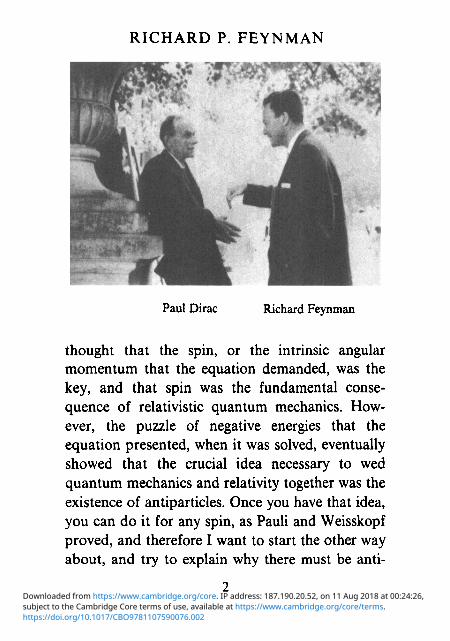
Paul Dirac Richard Feynman

thought that the spin, or the intrinsic angular momentum that the equation demanded, was the key, and that spin was the fundamental consequence of relativistic quantum mechanics. However, the puzzle of negative energies that the equation presented, when it was solved, eventually showed that the crucial idea necessary to wed quantum mechanics and relativity together was the existence of antiparticles. Once you have that idea, you can do it for any spin, as Pauli and Weisskopf proved, and therefore I want to start the other way about, and try to explain why there must be anti-

2


https://doi.org/10.1017/CBO9781107590076.002



The reason for antiparticles

particles if you try to put quantum mechanics with relativity.

Working along these lines will permit us to explain another of the grand mysteries of the world, namely the Pauli exclusion principle. The Pauli exclusion principle says that if you take the wave-function for a pair of spin \ particles and then interchange the two particles, then to get the new wavefunction from the old you must put in a minus sign. It is easy to demonstrate that if Nature was nonrelativistic, if things started out that way then it would be that way for all time, and so the problem would be pushed back to Creation itself, and God only knows how that was done. With the existence of antiparticles, though, pair production of a particle with its antiparticle becomes possible, for example with electrons and positrons. The mystery now is, if we pair produce an electron and a positron, why does the new electron that has just been made have to be antisymmetric with respect to the electrons which were already around? That is, why can't it get into the same state as one of the others that were already there? Hence, the existence of particles and antiparticles permits us to ask a very simple question: if I make two pairs of electrons and positrons and I compare the amplitudes for when they annihilate directly or for

3


https://doi.org/10.1017/CBO9781107590076.002



RICHARD P. FEYNMAN

when they exchange before they annihilate, why is there a minus sign?

All these things have been solved long ago, in a beautiful way which is simplest in the spirit of Dirac with lots of symbols and operators. I am going to go further back to Maxwell's 'gear wheels' and try to tell you as best I can a way of looking at these things so that they appear not so mysterious. I am adding nothing to what is already known; what follows is simply exposition. So here we go as to how things work-first, why there must be anti-particles.

RELATIVITY AND ANTIPARTICLES

In ordinary nonrelativistic quantum mechanics, if you have a disturbing potential U acting on a particle which is initially in a state 4>0, then the state will be different after the disturbance. Up to a phase factor and taking h = 1, the amplitude to end up in a state x is given by the projection of x onto U$0. In fact, we have:

A m P*„~x = -i/d3xX*£/<J»o= -i<x|tf|ft>>. (1)

The expression (xl^l^o) 1S Dirac's elegant bra and ket notation for amplitudes, although I will not use it much here. I will suppose though that

4


https://doi.org/10.1017/CBO9781107590076.002




this formula is true when we go to relativistic quantum mechanics.

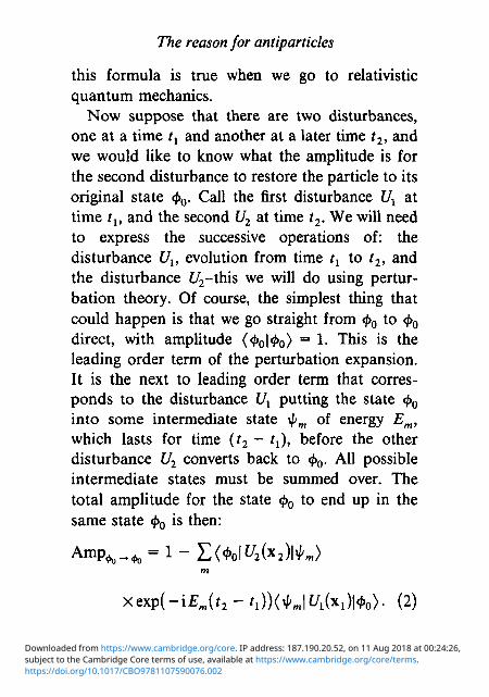
Now suppose that there are two disturbances, one at a time t1 and another at a later time t2, and we would like to know what the amplitude is for the second disturbance to restore the particle to its original state <J>0. Call the first disturbance Ux at time tv and the second U2 at time t2. We will need to express the successive operations of: the disturbance Ux, evolution from time tx to t2, and the disturbance £/2-this we will do using perturbation theory. Of course, the simplest thing that could happen is that we go straight from <>0 to <j>0

direct, with amplitude (<J>0|4>o) = 1- This is the leading order term of the perturbation expansion. It is the next to leading order term that corresponds to the disturbance Ux putting the state <>0

into some intermediate state i//m of energy Em, which lasts for time (t2 - tj, before the other disturbance U2 converts back to <>0. All possible intermediate states must be summed over. The total amplitude for the state <f>0 to end up in the same state <#>0 is then:

Amp^^l-L^ol^x^J m

xexp(-i£m(r2 - O X ^ J t A M ^ o ) - (2)


https://doi.org/10.1017/CBO9781107590076.002



RICHARD P. FEYNMAN

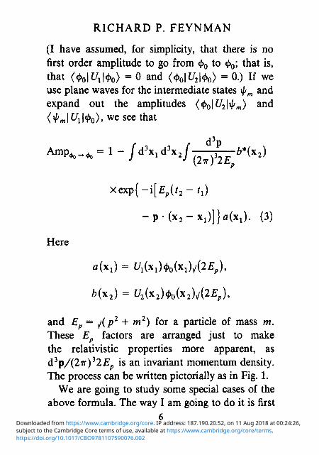
(I have assumed, for simplicity, that there is no first order amplitude to go from </>0 to <J>0; that is, that ( . y t / ^ o ) = 0 and (<t>0\U2\<j>0) = 0.) If we use plane waves for the intermediate states \pm and expand out the amplitudes (<j>0\U2\\pm) and ( ' / U ^ i K ) . we see that

/

t d3p d3x, d3x2 / \ b*(\7) 1 2J (2w)32Ep

V 2}

Xexp[-i[Ep(t2-tl)

- p - ( x 2 - x 1 ) ] } a ( x l ) . (3)

Here

fl(Xl) = UfaWiWEp)*

b(x2) = u2{x2)k>MA2Ep).

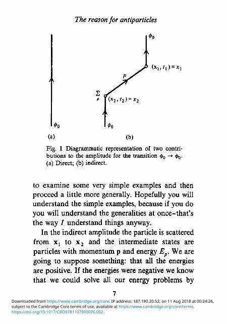
and Ep = j(p2 + m2) for a particle of mass m. These E factors are arranged just to make the relativistic properties more apparent, as d3p/(2ir)32Ep is an invariant momentum density. The process can be written pictorially as in Fig. 1.

We are going to study some special cases of the above formula. The way I am going to do it is first

6


https://doi.org/10.1017/CBO9781107590076.002




(xl>t1) = xi

(a) (b)

Fig. 1 Diagrammatic representation of two contributions to the amplitude for the transition <J>0 -* <J>0. (a) Direct; (b) indirect.

to examine some very simple examples and then proceed a little more generally. Hopefully you will understand the simple examples, because if you do you will understand the generahties at once-that's the way / understand things anyway.

In the indirect amplitude the particle is scattered from X! to x2 and the intermediate states are particles with momentum p and energy Ep. We are going to suppose something: that all the energies are positive. If the energies were negative we know that we could solve all our energy problems by

7


https://doi.org/10.1017/CBO9781107590076.002



RICHARD P. FEYNMAN

dumping particles into this pit of negative energy and running the world with the extra energy.

Now here is a surprise: if we evaluate the amplitude for any a ^ ) and b(x2) (we could even arrange for a(xj) and b(\2) to depend on p) we find that it cannot be zero when x2 is outside the light cone of \ v This is very surprising: if you start a series of waves from a particular point they cannot be confined to be inside the light cone if all the energies are positive. This is the result of the following mathematical theorem:

If a function f{t) can be Fourier decomposed into positive frequencies only, i.e. if it can be written

r e-,w'F(w)dw, (4) o

then / cannot be zero for any finite range of t, unless trivially it is zero everywhere. The vahdity of this theorem depends on F(u) satisfying certain properties, the details of which I would prefer to avoid.

You may be a bit surprised at this theorem because you know you can take a function which is zero over a finite range and Fourier analyze it, but

8


https://doi.org/10.1017/CBO9781107590076.002




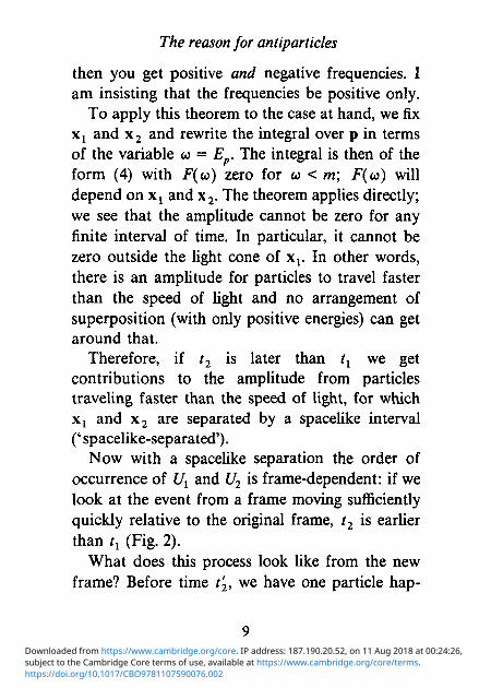
then you get positive and negative frequencies. I am insisting that the frequencies be positive only.

To apply this theorem to the case at hand, we fix xl and x2 and rewrite the integral over p in terms of the variable w = Ep. The integral is then of the form (4) with F(u) zero for w < m; F(u) will depend on xx and x2. The theorem applies directly; we see that the amplitude cannot be zero for any finite interval of time. In particular, it cannot be zero outside the light cone of xv In other words, there is an amplitude for particles to travel faster than the speed of light and no arrangement of superposition (with only positive energies) can get around that.

Therefore, if t2 is later than t1 we get contributions to the amphtude from particles traveling faster than the speed of light, for which Xj and x2 are separated by a spacelike interval (' spacelike-separated').

Now with a spacelike separation the order of occurrence of f/j and U2 is frame-dependent: if we look at the event from a frame moving sufficiently quickly relative to the original frame, t2 is earlier than tv (Fig. 2).

What does this process look like from the new frame? Before time t'2, we have one particle hap-

9


https://doi.org/10.1017/CBO9781107590076.002



RICHARD P. FEYNMAN

pily traveling along, but at time t'2 something seemingly very mysterious happens: at point x2, a finite distance from the original particle, the disturbance creates a pair of particles, one of which is apparently moving backwards in time. At time /{, the original particle and that moving backwards in time disappear. So the requirements of positive energies and relativity force us to allow creation and annihilation of pairs of particles, one of which travels backwards in time. The physical interpretation of a particle traveling backwards in time can most easily be appreciated if we temporarily give our particle a charge. In Fig. 2b, the particle travels from Xj to x2, bringing, say, positive charge from Xj to x2, yet since x2 occurs first it is seen as negative charge flowing from x2 to xx.

In other words, there must be antiparticles. In fact, because of this frame-dependence of the sequence of events we can say that one man's virtual particle is another man's virtual antiparticle.

To summarize the situation, we can make the following statements:

(1) Antiparticles and pair production and destruction must exist.

(2) Antiparticle behavior is completely determined by particle behavior.

10


https://doi.org/10.1017/CBO9781107590076.002




-»x

Light cone

00

0o (b)

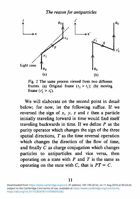
Fig. 2 The same process viewed from two different frames, (a) Original frame (f2 > tx)\ (b) moving frame (t'2 > t{).

We will elaborate on the second point in detail below; for now, let the following suffice. If we reversed the sign of x, y, z and t then a particle initially traveling forward in time would find itself traveling backwards in time. If we define P as the parity operator which changes the sign of the three spatial directions, T as the time reversal operation which changes the direction of the flow of time, and finally C as charge conjugation which changes particles to antiparticles and vice versa, then operating on a state with P and T is the same as operating on the state with C, that is PT = C.

11


https://doi.org/10.1017/CBO9781107590076.002



RICHARD P. FEYNMAN

SPIN-ZERO PARTICLES AND BOSE

STATISTICS

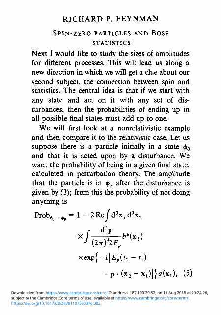
Next I would like to study the sizes of amphtudes for different processes. This will lead us along a new direction in which we will get a clue about our second subject, the connection between spin and statistics. The central idea is that if we start with any state and act on it with any set of disturbances, then the probabilities of ending up in all possible final states must add up to one.

We will first look at a nonrelativistic example and then compare it to the relativistic case. Let us suppose there is a particle initially in a state <j>0

and that it is acted upon by a disturbance. We want the probability of being in a given final state, calculated in perturbation theory. The amplitude that the particle is in <J>0 after the disturbance is given by (3); from this the probability of not doing anything is

P r o b^*„ = 1 - 2 R e / d 3 x i d 3 x 2

c d3p x / f—b*(\2)

Xexp{-i{Ep(t2-tl)

- p - ( x 2 - x1)]}a(x1), (5)


https://doi.org/10.1017/CBO9781107590076.002




using |1 + a\2 = 1 + a + a* + ••• = 1 + 2 Re a + ••• .

The amplitude that the particle is in state \pp

after the disturbance is

A m p ^ , = -i/d3x^(x)tf(x)<J>0(x). (6)

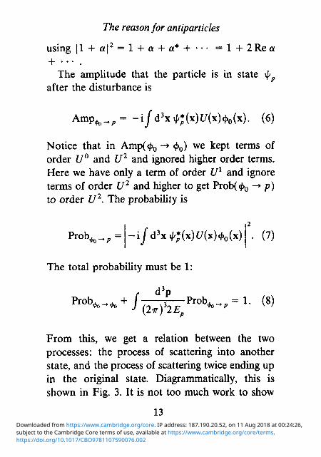
Notice that in Amp(4>0 -»<f>0) we kept terms of order U° and U2 and ignored higher order terms. Here we have only a term of order U1 and ignore terms of order U2 and higher to get Prob(<>0 -* p) to order U2. The probabihty is

P r o b _ = 't'o — P -i/d3x^(x)J7(x)<,0(x) • (7)

The total probability must be 1:

P r o b - - ° + / p^? r o b— " '• (8>

From this, we get a relation between the two processes: the process of scattering into another state, and the process of scattering twice ending up in the original state. DiagrammaticaUy, this is shown in Fig. 3. It is not too much work to show

13


https://doi.org/10.1017/CBO9781107590076.002



RICHARD P. FEYNMAN

2 2Re2 p

00

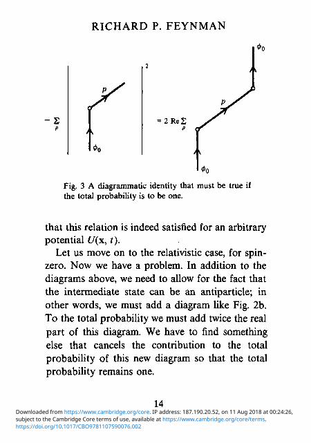
Fig. 3 A diagrammatic identity that must be true if the total probability is to be one.

that this relation is indeed satisfied for an arbitrary potential U(x, t).

Let us move on to the relativistic case, for spin-zero. Now we have a problem. In addition to the diagrams above, we need to allow for the fact that the intermediate state can be an antiparticle; in other words, we must add a diagram like Fig. 2b. To the total probability we must add twice the real part of this diagram. We have to find something else that cancels the contribution to the total probability of this new diagram so that the total probability remains one.

14


https://doi.org/10.1017/CBO9781107590076.002




2 * 2Re2 i

<f>o

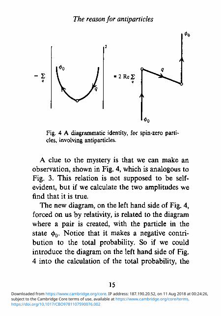
Fig. 4 A diagrammatic identity, for spin-zero particles, involving antiparticles.

A clue to the mystery is that we can make an observation, shown in Fig. 4, which is analogous to Fig. 3. This relation is not supposed to be self-evident, but if we calculate the two amplitudes we find that it is true.

The new diagram, on the left hand side of Fig. 4, forced on us by relativity, is related to the diagram where a pair is created, with the particle in the state 4>0. Notice that it makes a negative contribution to the total probability. So if we could introduce the diagram on the left hand side of Fig. 4 into the calculation of the total probabiUty, the

15


https://doi.org/10.1017/CBO9781107590076.002



RICHARD P. FEYNMAN

total probability would turn out to be one and we would have the problem solved.

However, simply including this diagram makes no sense, for a couple of reasons. First, the diagram on the left hand side of Fig. 4 starts from a different initial state (the vacuum rather than <f>0); and, second, there seems to be no reason to restrict ourselves to pair creation with the particle in state <f>0-any particle state is possible. We get the correct answer, but for the wrong reason.

What I have told you so far is the truth but not the whole truth. We have neglected several diagrams, and when it is all put together we will get an important feature of Bose statistics: that when a particle is in a certain state the probability of producing another particle in that state is enhanced.

Let us take one step back: instead of starting with a particle in <J>0 let us start in the vacuum V (i.e. the no-particle state), and examine our familiar idea that the total probability must be one. In the nonrelativistic case this would have been a trivial exercise: starting with no particles nothing could happen, and the probability of nothing happening would be one. In the relativistic case; on the other hand, we have seen that pair creation and annihilation must be included. Because of this, the

16


https://doi.org/10.1017/CBO9781107590076.002




(Vacuum-vacuum)

(a)

(b) (c)

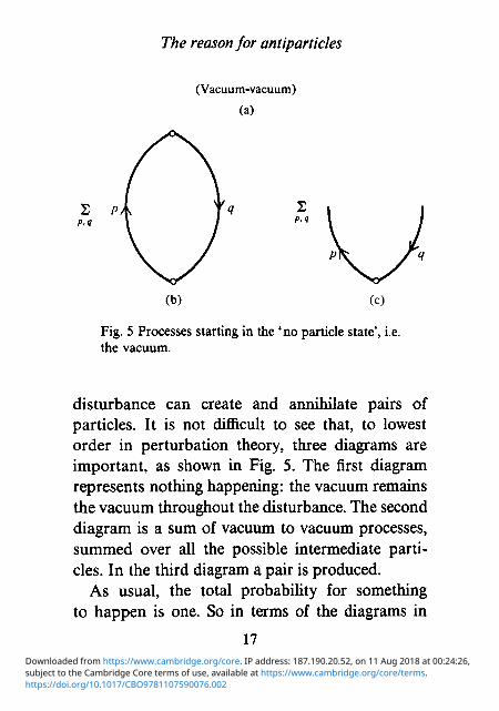
Fig. 5 Processes starting in the 'no particle state', i.e. the vacuum.

disturbance can create and annihilate pairs of particles. It is not difficult to see that, to lowest order in perturbation theory, three diagrams are important, as shown in Fig. 5. The first diagram represents nothing happening: the vacuum remains the vacuum throughout the disturbance. The second diagram is a sum of vacuum to vacuum processes, summed over all the possible intermediate particles. In the third diagram a pair is produced.

As usual, the total probability for something to happen is one. So in terms of the diagrams in

17


https://doi.org/10.1017/CBO9781107590076.002



RICHARD P. FEYNMAN

2

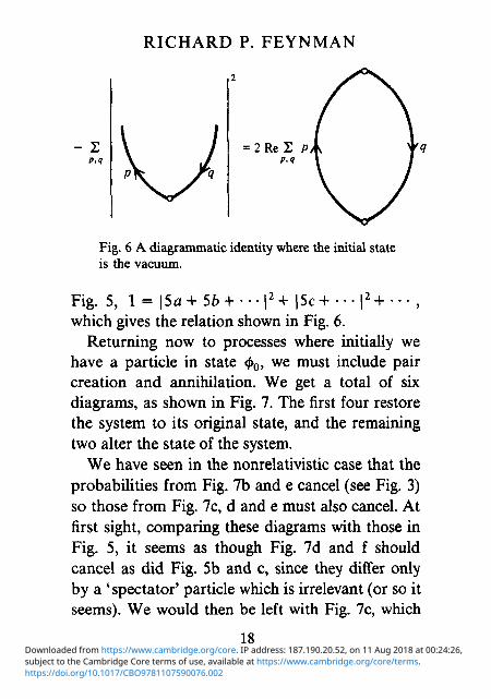
Fig. 6 A diagrammatic identity where the initial state is the vacuum.

Fig. 5, 1 = \5a + 5b+---\2+ |5c+ • • • | 2 + - - - , which gives the relation shown in Fig. 6.

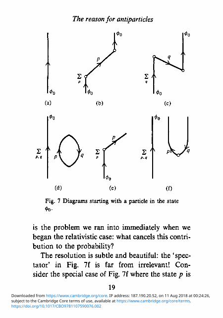
Returning now to processes where initially we have a particle in state <J>0, we must include pair creation and annihilation. We get a total of six diagrams, as shown in Fig. 7. The first four restore the system to its original state, and the remaining two alter the state of the system.

We have seen in the nonrelativistic case that the probabilities from Fig. 7b and e cancel (see Fig. 3) so those from Fig. 7c, d and e must also cancel. At first sight, comparing these diagrams with those in Fig. 5, it seems as though Fig. 7d and f should cancel as did Fig. 5b and c, since they differ only by a 'spectator' particle which is irrelevant (or so it seems). We would then be left with Fig. 7c, which

18


https://doi.org/10.1017/CBO9781107590076.002




(a) (b)

2 * <7

00

(c)

2

(d) (e)

2 P N y / ^

(0

Fig. 7 Diagrams starting with a particle in the state <f>o-

is the problem we ran into immediately when we began the relativistic case: what cancels this contribution to the probability?

The resolution is subtle and beautiful: the 'spectator' in Fig. 7f is far from irrelevant! Consider the special case of Fig. 7f where the state p is

19


https://doi.org/10.1017/CBO9781107590076.002



RICHARD P. FEYNMAN

h |0o I i0o 0O I

+

Fig. 8 One of the diagrams from Fig. 7f, with the exchange diagram.

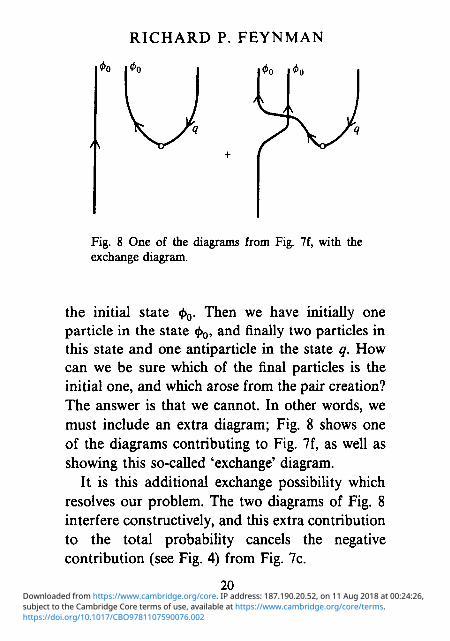
the initial state <|>0. Then we have initially one particle in the state 4>0, and finally two particles in this state and one antiparticle in the state q. How can we be sure which of the final particles is the initial one, and which arose from the pair creation? The answer is that we cannot. In other words, we must include an extra diagram; Fig. 8 shows one of the diagrams contributing to Fig. 7f, as well as showing this so-called 'exchange' diagram.

It is this additional exchange possibility which resolves our problem. The two diagrams of Fig. 8 interfere constructively, and this extra contribution to the total probability cancels the negative contribution (see Fig. 4) from Fig. 7c.

20


https://doi.org/10.1017/CBO9781107590076.002




So let me summarize the situation. We've added a few extra diagrams to account for the fact that pair production can occur; in particular we've had to add the diagram in Fig. 7c. We discovered that when we try to check the sum of the probabilities, this diagram (Fig. 7c) makes a negative contribution to the total probabihty, which must cancel something. What it cancels is an extra probability for producing, in the presence of a 'spectator' particle, the special particle-antipar-ticle pair where the newly produced particle is in the same state as the 'spectator'.

This enhanced probabihty is a very profound and important result. It says that the mere presence of a particle in a given state doubles the probability to produce a pair, the particles of which are in that same state. If there are n particles initially in that state, the probabihty is increased by a factor n + 1. This can obviously become very important! This is a key feature of Bose statistics, which makes the laser work, among other things.

As another example, let's look at some higher order vacuum-to-vacuum diagrams. Suppose the disturbing potential acts four times, producing and annihilating two particle-antiparticle pairs, as in Fig. 9a. Now suppose you compared that to what would happen if you produced the pairs and each

21


https://doi.org/10.1017/CBO9781107590076.002



RICHARD P. FEYNMAN

00 CO (a) (b)

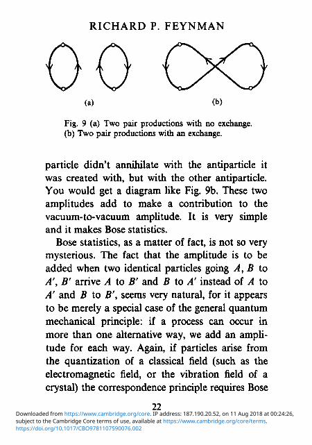
Fig. 9 (a) Two pair productions with no exchange, (b) Two pair productions with an exchange.

particle didn't annihilate with the antiparticle it was created with, but with the other antiparticle. You would get a diagram like Fig. 9b. These two amplitudes add to make a contribution to the vacuum-to-vacuum amplitude. It is very simple and it makes Bose statistics.

Bose statistics, as a matter of fact, is not so very mysterious. The fact that the amplitude is to be added when two identical particles going A, B to A', B' arrive A to B' and B to A' instead of A to A' and B to B', seems very natural, for it appears to be merely a special case of the general quantum mechanical principle: if a process can occur in more than one alternative way, we add an amplitude for each way. Again, if particles arise from the quantization of a classical field (such as the electromagnetic field, or the vibration field of a crystal) the correspondence principle requires Bose

22


https://doi.org/10.1017/CBO9781107590076.002




particles if intensity correlations are to be correct, such as in the Hanbury Brown Twiss Effect.* More simply the field mode harmonic oscillators, when quantized, automatically imply a representation as Bose particles.

What we will find out later is that for fermions, particles with half-integral spin, unexpected minus signs arise. In the case of Fig. 9, for example, each loop gives the amplitude a minus sign. Therefore Fig. 9a has two minus signs, whereas Fig. 9b (which has only one loop) has one minus sign, so the amplitudes subtract and you get Fermi statistics. We are going to have to understand why with spin \ there is a minus sign for each loop. The key is that there are implicit rotations by 360°, as we shall see.

THE RELATION OF PARTICLE AND

ANTIPARTICLE BEHAVIOR

Before we talk about fermions, I would like to return to explain in a bit more detail the relationship between particle behavior and anti-particle behavior. Of course, the antiparticle

* R. P. Feynman (1962). Theory of Fundamental Processes, pp. 4-6,

W. A. Benjamin.

23


https://doi.org/10.1017/CBO9781107590076.002



RICHARD P. FEYNMAN

behavior is completely determined by the particle behavior. Let me analyze this more carefully in the simplest case of spin-zero and scalar potentials U. We have seen that for t2 > tx the amplitude for a free particle of mass m to go from xx to x2 is

, d3p F{2>l) = hn^7 J (2w) 2Ep

Xexp{-i[Ep{t2- tx) - p - ( x 2 - X l ) ] } .

(9)

This formula is relativistically covariant, so for spin-zero we may take a, b constant in (5). We want to know what the amplitude is for t2 < tv

For t2< tx and spacelike separation, the answer is easy: the amplitude is still F(2,1). This is because we know F(2,1) is correct in the spacelike region for t2 > tv but if we look at such a process in a different frame, it must always be spacelike but we can have t2 < tv In that frame we would get the same amplitude-it can't depend upon which frame we're in-and when we try to write F(2,1) in terms of the transformed frame's coordinates we get the same formula because .F(2,1) is relativistically covariant. So F(2,1) is the correct formula for the

24


https://doi.org/10.1017/CBO9781107590076.002




amplitude in either the forward light cone or in the spacelike region. What about the backward light cone?

The other piece of information we need is that for t2< tx we are still propagating only positive energies. Therefore in this region we must be able to write the amplitude in the form

G(2 , l )= r e+ i ^ - ' ' )

X ( x 1 , x 2 , ( o ) d c o ) (10) •'o

where x is some function we want to determine. The reason for the change of sign in the exponential is as follows. We are creating waves at xv which we insist contain only positive energies or frequencies as we leave the source. In other words, the time dependence must be exp(-iwAr) with w > 0. Here At is the time away from the source, which must be positive. For t2 > tl the waves have existed for time At = t2 - tx; for t2 < t1 the waves have existed for time At = t1 — t2.

So for t2 < tv whether in the past light cone or the spacelike region, we must be able to write the amplitude in the form of (10). This means that when t2 < tx in the spacehke region, we could use either (9) or (10) to obtain the amplitude. This is going to determine G in that region, and it will then extrapolate uniquely for all t2 < tv

25


https://doi.org/10.1017/CBO9781107590076.002



RICHARD P. FEYNMAN

For t2< tx and xt and x2 spacelike separated, we have an expression (9) which is a sum of negative frequencies. The question is, can we also express it as a function of positive frequencies alone? Ordinarily you can't do it. It's magic, but for this particular function which is relativistically invariant it is possible. Let me show you why.

First, for tx = t2, F(2,1) is real. In that case the exponential is just exp[ip • (x2 - \x)] and the imaginary part is an odd function integrated over an even domain, which is zero. But if F is real for tl = t2 then it must be real for any tx and t2 with spacelike separation by relativistic invariance: a moving observer would calculate the same real amplitude, yet to him t2 ¥= tx. Since it is real it is equal to its complex conjugate, which has the opposite-sign time dependence. So a solution for G(2,1) is the complex conjugate of F{2,1):

, d3p

Xexp{+i[£„(f2 - h) - p • (x2 - X l)]}.

(11)

This has the correct form: it propagates only positive energies. This must be the unique solution, for

26


https://doi.org/10.1017/CBO9781107590076.002




no function of type (10) can differ from this solely in the backward light cone, by theorem (4). So if t2

is above tx in the forward light cone, the answer is equation (9); if /2 is below tx in the backward light cone the answer is equation (11); and in the intermediate region where tx and t2 are spacelike separated the answer is either (9) or (ll)-they're equal!

We started by knowing something in one region of spacetime, and, just by supposing that it is relativistically invariant, we were able to deduce what happens all over spacetime. That's not so mysterious. If we knew something in just one region of a four-dimensional Euclidean space, but knew its rotational transformation properties (in our example, the function is invariant) we could rotate our region in any direction and watch things change in some well-defined way; then we could work things out all over our Euclidean four-space. Here we have four-dimensional Minkowski space-time, x, y, z and t, which is a little different-but not that much; we can still do it. The difficulty with Minkowski space is that there is a kind of no-man's land where t2 is outside the light cone of tx\ the Lorentz transformations can't really move through there. But we have obtained the correct continuation across this spacelike region because

27


https://doi.org/10.1017/CBO9781107590076.002



RICHARD P. FEYNMAN

supposing the energies are always positive limits the solution. In other words this operation PT which changes the sign of everything is really a relativistic transformation, or rather a Lorentz transformation, extended across the spacelike region by demanding that the energy is greater than zero. So it is not so mysterious that relativistic invariance produces the whole works.

SPIN \ AND FERMI STATISTICS

So that was spin-zero, and now I would like to do spin \ and see what happens. If you have a spin \ state and you rotate it about, say, the z-axis by an angle 8, then the phase of the state changes by e-i0/2 There is a whole mass of group theoretic arguments to prove this sort of thing which I won't go into now, although it's a lovely exercise. The point is that if you rotate by 360° then you end up multiplying the wavefunction by (-1). At this point all attempts to do anything by instinct fail, because this result is hard to understand. How can a complete 360° rotation change anything? One of the hardest things now will be to keep track of whether you've made a 360° rotation or not, i.e. whether you should include the minus sign or not. In fact, as we shall see, the mysterious minus signs

28


https://doi.org/10.1017/CBO9781107590076.002




in the behavior of Fermi particles are really due to unnoticed 360° rotations!

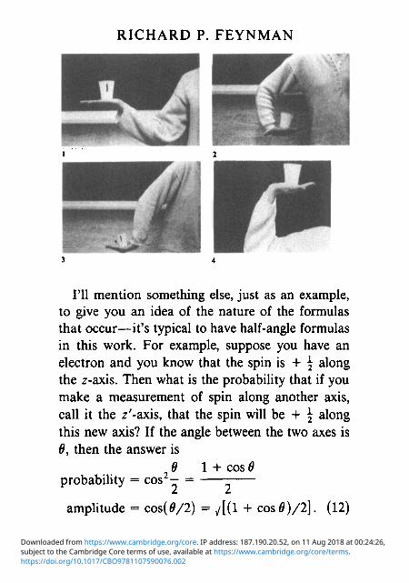
Dirac had a very nice demonstration of this fact-that rotation one time around can be distinguished from doing nothing at all.* In fact, it's rotation twice around that is about the same as doing nothing. I'll show you something you can find dancing girls doing! Here-I am going to rotate this cup (see photograph sequence overleaf), remember which way, all the way around until you can see the mark again, and now I have rotated 360°, but I'm in trouble. However, if I continue to rotate it still further, which is a nervy thing to do under the circumstances, I do not break my arm, I straighten everything out. So two rotations are equivalent to doing nothing, but one rotation can be different, so you have to keep track of whether you've made a rotation or not, and the rest of this talk is a nerve racking attempt to try to keep track of whether you've made a rotation or not*.

* For this demonstration due to Dirac, his famous scissors demonstration, see R. Penrose and W. Rindler (1984). Spinors and Space-lime, vol. 1, p. 43. Cambridge University Press.

+ This was taken verbatim from Feynman's lecture.

29


https://doi.org/10.1017/CBO9781107590076.002



RICHARD P. FEYNMAN

I'll mention something else, just as an example, to give you an idea of the nature of the formulas that occur—it's typical to have half-angle formulas in this work. For example, suppose you have an electron and you know that the spin is + ^ along the z-axis. Then what is the probability that if you make a measurement of spin along another axis, call it the z'-axis, that the spin will be + \ along this new axis? If the angle between the two axes is 6, then the answer is

0 1 + cos 0 probability = cos2— =

amplitude = cos(0/2) = j[(l + cos0)/2]. (12)


https://doi.org/10.1017/CBO9781107590076.002




Now we are going to study amplitudes in a spin \ theory with a scalar coupling. This means the disturbance, U, will be as simple as possible so that the spin parts of the amplitudes arise from the particles themselves, not from the disturbance, which will make the analysis easier. We will get formulas like the half-angle formula above, except with a relativistic modification. Here we go.

If we have a particle of mass m we know that the energy and momentum must satisfy:

E2-p2 = m2. (13)

m2 is just a constant, of course, and p = |p| is the magnitude of the momentum. This means that given E, p is determined and vice versa, so we don't need two different variables. Now (13) looks like the trigonometry formula cos20 + sin20 = l, except for the factor m2 and a minus sign. We can use the hyperbolic functions rather than trigonometric functions to parametrize E and p in terms of just one variable. If we write

E = wcoshw,

p = wsinhw, (14)

then E and p automatically satisfy (13): w is our new variable. It's called the rapidity.

31


https://doi.org/10.1017/CBO9781107590076.002



RICHARD P. FEYNMAN

Suppose we have a particle at rest in a given spin state and that the disturbance puts the particle into a state with momentum p. The initial momentum four-vector is px = (m, 0,0,0), and the final one is say p2- (E, p,0,0) with E and p as in (14). The amplitude for this scattering process is given by a sort of half-angle formula analogous to (12); up to irrelevant factors it is

A^ a cosh(w/2). (15)

In analogy to the spatial rotation case above, we can write this, again up to irrelevant factors, as

Acatt a y(coshw + 1) a j(E + m). (16)

We can uniquely write this amplitude in a relativistically covariant way by noting that px • p2

= Em, where pl • p2 is the dot product of the two four-vectors. The amplitude can therefore be written:

^sca.t «APl-P2 + ™2)- (17)

The power of rewriting it in a relativistically covariant way is that this amplitude, which we came up with in a special case, is now valid for any Pit Pi- We are going to use it to derive the ampli-

32


https://doi.org/10.1017/CBO9781107590076.002




tude for pair production. Suppose we choose px = (m, 0,0,0) as before, but p2 = (-E, -p, 0,0). This negative energy state represents an antiparticle, of course. Now px • p2 = —Em and we get:

Apairccj(-mE + m2)ay(E-m) (18)

as the amplitude for pair production. Using these results, we are going to modify our

discussion of total probabilities above to the case of spin \, and we will see that we are forced to invoke the Pauli exclusion principle. The discussion is quite similar to the spin zero case, so I will concentrate mainly on the difference between spin-zero and spin \.

If we study processes starting from the vacuum, the spin-zero discussion carries over directly and we get the relation shown in Fig. 6.

Let us now study processes starting from a particle in the state <>0, which we now take to be a particle at rest. We get the same six diagrams as in Fig. 7, but this time the amplitudes among related diagrams obey drastically different relations.

For the total probability, we are interested in the real part of Fig. 7b, c, and d, and the absolute square of Fig. 7e and f. Let us start with Fig. 7b. In this process the particle scatters into the state p

33


https://doi.org/10.1017/CBO9781107590076.002



RICHARD P. FEYNMAN

at xv and propagates to x2, where it scatters back into the state </>0. From (17) we know the scatterings give a factor ^(E + m) each, so the amplitude for Fig. 7b is:

t d3P / b J (27r)32£/ ' '

Xexp{-i[Ep(t2- tx) - p - ( X J - X J ) ] } ,

(19)

where the minus sign comes from the factors - i at each vertex.

The probability for the scattering process in Fig. 7e is given by the absolute square of (16), so summing over momenta it turns out that (16) and (19) imply that the relation shown in Fig. 3 holds for spin \ particles as well.

We must now be careful to obtain the correct expression for Fig. 7c. It must be an expression with negative frequencies equal to (19) when r2,x2

and tv Xj are spacelike separated. But (19) evidently equals -[m + i(d/dt2)F(2,l)] (see (7)), which equals -[m + \{d/dt2)G{2,1)] in the

34


https://doi.org/10.1017/CBO9781107590076.002




spacelike region so Fig. 7c must be, uniquely,

Xexp{+i[£p(f2 - tx) - p • (x2 - xx)]}.

(20)

This has been obtained by analytic continuation arguments (as in the derivation of (11)), without using (18), although the factor (-E+ m) may also be thought of as arising from two factors of Apair (see (18)).

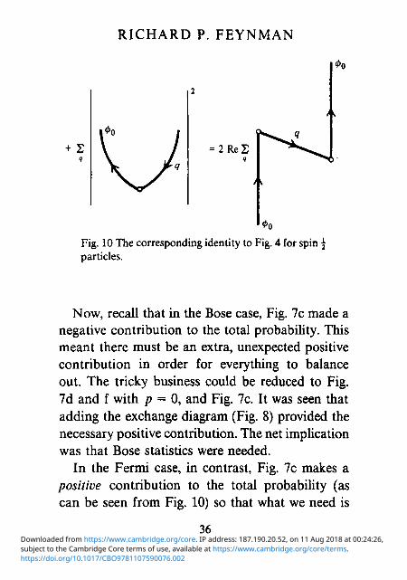
The important difference between the spin \ and spin-zero cases occurs at this point: the relation shown in Fig. 4 is false for fermions. To see this for the spin \ case we have all the necessary ingredients. From (18) we get E - m for the necessarily positive probability of pair production; comparing this with the real part of the amplitude (20) (which has a factor —E + m times the spin-zero amplitude) we get the relation shown in Fig. 10, which differs from Fig. 4 by a crucial minus sign.

35


https://doi.org/10.1017/CBO9781107590076.002



RICHARD P. FEYNMAN

+ 2 = 2 Re 2 9

00

Fig. 10 The corresponding identity to Fig. 4 for spin \ particles.

Now, recall that in the Bose case, Fig. 7c made a negative contribution to the total probability. This meant there must be an extra, unexpected positive contribution in order for everything to balance out. The tricky business could be reduced to Fig. 7d and f with p = 0, and Fig. 7c. It was seen that adding the exchange diagram (Fig. 8) provided the necessary positive contribution. The net impUcation was that Bose statistics were needed.

In the Fermi case, in contrast, Fig. 7c makes a positive contribution to the total probability (as can be seen from Fig. 10) so that what we need is

36


https://doi.org/10.1017/CBO9781107590076.002




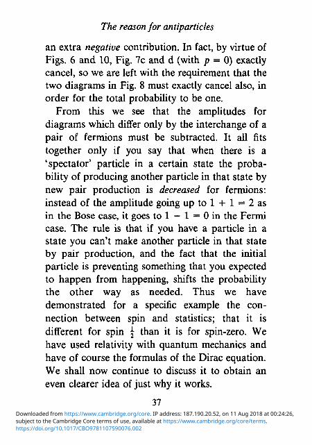
an extra negative contribution. In fact, by virtue of Figs. 6 and 10, Fig. 7c and d (with p = 0) exactly cancel, so we are left with the requirement that the two diagrams in Fig. 8 must exactly cancel also, in order for the total probability to be one.

From this we see that the amplitudes for diagrams which differ only by the interchange of a pair of fermions must be subtracted. It all fits together only if you say that when there is a 'spectator' particle in a certain state the probability of producing another particle in that state by new pair production is decreased for fermions: instead of the amplitude going up to 1 + 1 = 2 as in the Bose case, it goes to 1 — 1 = 0 in the Fermi case. The rule is that if you have a particle in a state you can't make another particle in that state by pair production, and the fact that the initial particle is preventing something that you expected to happen from happening, shifts the probability the other way as needed. Thus we have demonstrated for a specific example the connection between spin and statistics; that it is different for spin \ than it is for spin-zero. We have used relativity with quantum mechanics and have of course the formulas of the Dirac equation. We shall now continue to discuss it to obtain an even clearer idea of just why it works.

37


https://doi.org/10.1017/CBO9781107590076.002



RICHARD P. FEYNMAN

ANTIPARTICLES AND TIME REVERSAL

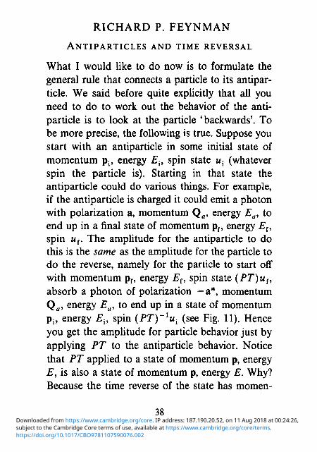
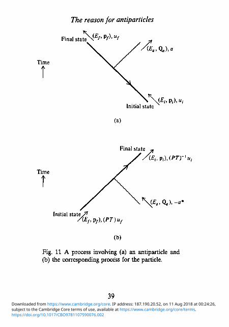
What I would like to do now is to formulate the general rule that connects a particle to its antipar-ticle. We said before quite explicitly that all you need to do to work out the behavior of the anti-particle is to look at the particle 'backwards'. To be more precise, the following is true. Suppose you start with an antiparticle in some initial state of momentum pi5 energy Ev spin state u{ (whatever spin the particle is). Starting in that state the antiparticle could do various things. For example, if the antiparticle is charged it could emit a photon with polarization a, momentum Qa, energy Ea, to end up in a final state of momentum pf, energy E(, spin u{. The amplitude for the antiparticle to do this is the same as the amplitude for the particle to do the reverse, namely for the particle to start off with momentum pf, energy E{, spin state (PT)us, absorb a photon of polarization - a*, momentum Qa, energy Ea, to end up in a state of momentum pi( energy E{, spin (PT)~lui (see Fig. 11). Hence you get the amplitude for particle behavior just by applying PT to the antiparticle behavior. Notice that PT applied to a state of momentum p, energy E, is also a state of momentum p, energy E. Why? Because the time reverse of the state has momen-

38


https://doi.org/10.1017/CBO9781107590076.002




Final state\C £>, p ' ) , M'

Time r AE.,0.),

. \(£/> p,0, u, Initial state

(a)

Time

Final state

(PTy'ui

\E„,Qa),-a*

Initial state le/l AEf,pf),(PT)uf

(b)

Fig. 11 A process involving (a) an antiparticle and (b) the corresponding process for the particle.

39


https://doi.org/10.1017/CBO9781107590076.002



RICHARD P. FEYNMAN

turn - p , energy E, but then applying parity and reversing all spatial directions puts it back to momentum p, energy E. PT does affect the polarization of the photon though, and also the spin states. Note that at one end of the process we must make the inverse transformation, i.e. a (PT)~l transformation. Although this sounds the same as PT, there is a subtle difference as we shall see in a minute. Hence the C that changes from particle to antiparticle is equivalent to a parity reversal P together with a time reversal T. Everything is done in the reverse order in time-for example, if you have circularly polarized light, the polarization vector is say (ex, ey) = (1, i), the time reversed polarization is (ex, ey)* = (1, — i) which has the electric vector going round in the reverse direction. Then PT(ex,ev) = -(ex,ey)* and so on. C = Pr-everything backwards in time and reversed in space. I'm not going to go through the details to prove it though.

As mentioned above, when getting the particle behavior from the antiparticle, one spin state at one end has PT applied, the other at the other end has (PT)'1 applied. We would prefer to have the same transformation applied to both, because if the spin states «j and u{ are the same, then so are the spin states (PT)u{ and (PT)u(. We will need

40


https://doi.org/10.1017/CBO9781107590076.002




to use this later. It turns out that there is no problem with the parity operation P, so let us choose the phases so that P2 = 1, i.e. two space inversions is the same as doing nothing. What we are going to show though is that for spin \ particles T~l = -T, i.e. that TT = - 1 , whereas for spin-zero TT = +1. That difference in sign, that extra minus sign, is where the Pauli exclusion principle and Fermi statistics come from.

THE EFFECT OF TWO SUCCESSIVE

TIME REVERSALS

Why should it be that two time reversals change the sign of a spin \ particle? The answer is that changing T twice is equivalent to a 360° rotation. If I flipped the jc-axis twice, I would be rotating through 360°, and thinking in four-dimensional spacetime; the same could be true of the /-axis too. Indeed it is true as I will demonstrate below (even without implying any relativistic relation of t and x!). Then, as we said above, rotating a spin \ particle by 360° multiplies it by (-1), so we find TT = - 1 . Let's show that we must have TT = - 1 for spin \.

In Table 1 are listed various states, together with what you get if you apply T once, and then once

41


https://doi.org/10.1017/CBO9781107590076.002



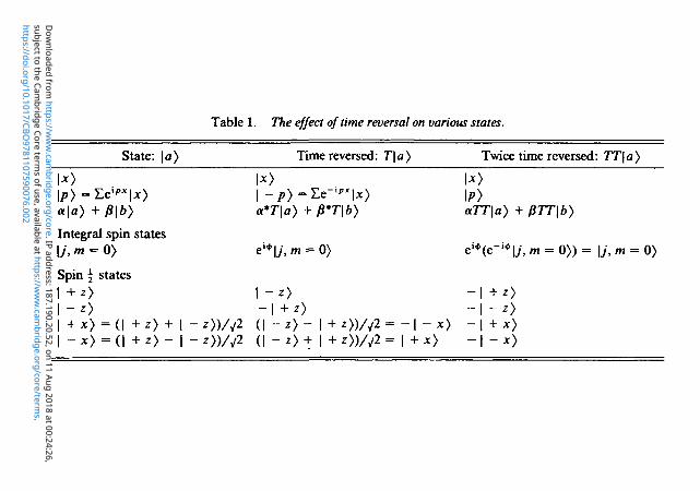
Table 1. The effect of time reversal on various states.

State: \a)

\p)=Le^\x) a\a) + 0\b)

Integral spin states \j, m = 0)

Spin \ states I + ' > I " * > | + x ) - ( | + z > + | - z » / V 2 | - x) = (| + z) - | - z » / / Z

Time reversed: T\a)

\ - p) =Le-""\x) a*T\a) + P*T\b)

ei*|7,m = 0)

- | + z ) ( | - 2 > - | + 2 » / V 2 = - | -JC> (| - 2) + | + 2»/ /> = | + *>

Twice time reversed: TT\a)

I/O «7T|a> + /S7T|A>

ei*(e-i*|y,W = 0 » = |y,m = 0>

-I +0 - | - 2 )

- | + x > - | - x >

https://doi.org/10.1017/CBO9781107590076.002

subject to the Cambridge Core term

s of use, available at https://ww

w.cam

bridge.org/core/terms.

Dow

nloaded from https://w

ww

.cambridge.org/core. IP address: 187.190.20.52, on 11 Aug 2018 at 00:24:26,

https://doi.org/10.1017/CBO9781107590076.002




more. The first state is the state where a particle is at the point x in space; this state is written \x) using Dirac's notation. In between the ' | ' and the ' ) ' one puts the name of the state, or just something to label it, which in this case is the point x where the state is. Then the time reversed state is T\x) = \x), i.e. the particle will be at the same point, no big deal. On the other hand, a particle in a state of momentum p (i.e. in a state \p)) will time reverse into a state of momentum —p, but then back to \p) with the second time reversal.

Considering the state \p) shows us that T is what is called an 'antiunitary' operation. \p) can be made by combining states \x) at different positions with different phases. To get the time reversed state | — p) just take the states T\x) = \x) but with the complex conjugate of the phases used to construct \p). So in general T[a\a) + P\b)] = a*T\a) + p*T\b), i.e. for an antiunitary operation you must take the complex conjugates of the coefficients whenever you see them. Of course, if you apply T again, you take the complex conjugate of the coefficients again, and if you are very good at algebra you know that doing that is a waste of time. Now TT\a) must be the same physical state |a>, but the damn quantum mechanics always allows you to have a different

43


https://doi.org/10.1017/CBO9781107590076.002



RICHARD P. FEYNMAN

phase. So, by the above argument, TT\a) = phase \a) with the same phase for all states that could be superposed with the state \a), so that any interference between states is the same before and after applying TT. Spin-zero and spin ^ states cannot be superposed, the two sorts of state are fundamentally different; hence the overall phase change when you apply TT can be different between the two.

What we are going to use now is that if you have a state of angular momentum \j,m), then T\j, m) = phase [/', —m). It must be like this for angular momentum: the time reverse of something spinning one way is the object spinning in the opposite direction. For example, with orbital angular momentum L = r A p, we find that since T sends r -» r and p -» - p, then 7T = - L, i.e. you get the opposite angular momentum when you apply T.

First of all consider integral spin states. There will be a state with no z-angular momentum, namely [/, m — 0). Applying one T this becomes the same state [/, m = 0) times some phase, but applying T again can only put the state back to exactly [/', m = 0), using the fact that T is antiunitary. So since the phase is the same for all

44


https://doi.org/10.1017/CBO9781107590076.002




states that can be superposed, TT = +1 for integral spin states.

To understand what happens with half integral spin let us take the simplest example of spin \. Let us try to fill out our table for just the four special states, up and down along the z-axis, | + z), | — z), and up and down along the x-axis | + x), | — x). Elementary spin theory tells us how these latter two can be expressed in terms of the | + z) and | - z) base states: one of them, | 4- x), is the in-phase equal superposition, and the other, | - x), is the out-of-phase equal superposition. The physically time reversed state of | + z) is | - z) and vice versa. Likewise, time reversal of | + x) must send us to | — x) within a phase.

For our first entry T\ + z) we must have \ — z), at least within a phase. This first phase can be chosen arbitrarily, as you can check later, so we may as well take T\ + z) = | - z). Now T\ - z) must be a phase times \ + z). But we cannot choose it to be simply \ + z) because then the operation of r on | + x), the in-phase superposition of | + z) and | - z), will only give back the same in-phase state | + x) and not a factor times the out-of-phase state | - x), as it physically must. To make this phase reversal occur we must

45


https://doi.org/10.1017/CBO9781107590076.002



RICHARD P. FEYNMAN

take T\ — z) = — | + z), of opposite phase from what we did for T\ + z). Now T(T\ + z» = T\ - z) = - | + z) and the rest of the table can be filled out. Therefore TT = - 1 for spin \, as is easily shown for any half integral spin j , where time reversal never brings us back to the same physical state. Hence combining this with the result for integral spin particles, we have TT = 360° rotation.

Now we come to the sign of the spin \ loop. You will recall that, with a potential in relativistic quantum mechanics, pairs can be produced so the probability for the vacuum (i.e. the no particle state) to remain the vacuum must be less than one. Write the amplitude for the vacuum remaining the vacuum as 1 + X, where X is the contribution from all the closed loops drawn on the right hand side of Fig. 6. Then X must contribute a negative amount to the probability for the vacuum to remain the vacuum, which is what the identity in Fig. 6 says because the left hand side is strictly negative.

Consider the loops contributing to X. A loop is constructed by starting with an electron, for example, in a state with Dirac wavefunction u, say, and then propagating around the loop to come back into the same physical state u, and we must take the trace of the resulting matrix product,

46


https://doi.org/10.1017/CBO9781107590076.002




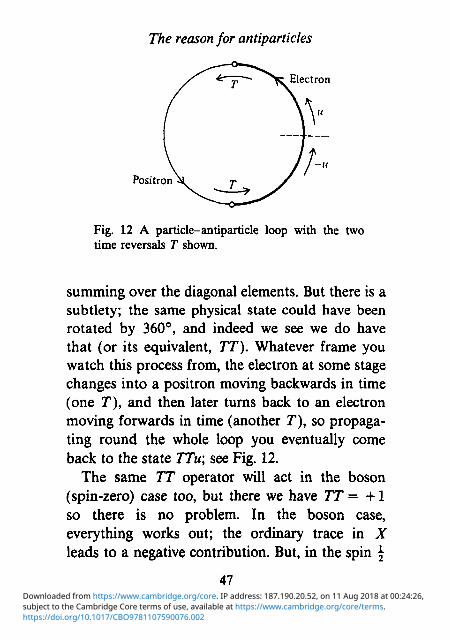
Fig. 12 A particle-antiparticle loop with the two time reversals T shown.

summing over the diagonal elements. But there is a subtlety; the same physical state could have been rotated by 360°, and indeed we see we do have that (or its equivalent, TT). Whatever frame you watch this process from, the electron at some stage changes into a positron moving backwards in time (one T), and then later turns back to an electron moving forwards in time (another T), so propagating round the whole loop you eventually come back to the state TTu; see Fig. 12.

The same TT operator will act in the boson (spin-zero) case too, but there we have TT = +1 so there is no problem. In the boson case, everything works out; the ordinary trace in X leads to a negative contribution. But, in the spin \

47


https://doi.org/10.1017/CBO9781107590076.002



RICHARD P. FEYNMAN

case, we have just found an extra minus sign. So to ensure the identity in Fig. 6 is true, to ensure that X leads to a negative contribution to the probability, we must add a new rule for half integral spin: with every ordinary loop trace we must associate an extra minus sign to compensate for the minus sign coming from TT = - 1 . If we don't put in this extra minus sign our probabilities won't add up, we won't have a consistent theory of spin \ particles. This sign is only consistent with Fermi statistics.

This general rule for spin \ loops, that for each closed loop you must multiply by — 1, is why we have Fermi statistics; see Fig. 9. There is a relative minus sign between the two cases in Fig. 9a and b, because Fig. 9a has two loops, whereas Fig. 9b only has one loop. Fig. 9 thus says that when swapping two particles around you must introduce a relative minus sign, i.e. Fermi statistics!

MAGNETIC MONOPOLES, SPIN AND

FERMI STATISTICS

Finally, to elucidate still more clearly the relation of the rotation properties of particles and their statistics, I would Uke to show you an example in which we have a spin \ object for which we know

48


https://doi.org/10.1017/CBO9781107590076.002




/ ' Electric charge q Q

/ / = W = » / 2

Magnetic monopole \i •

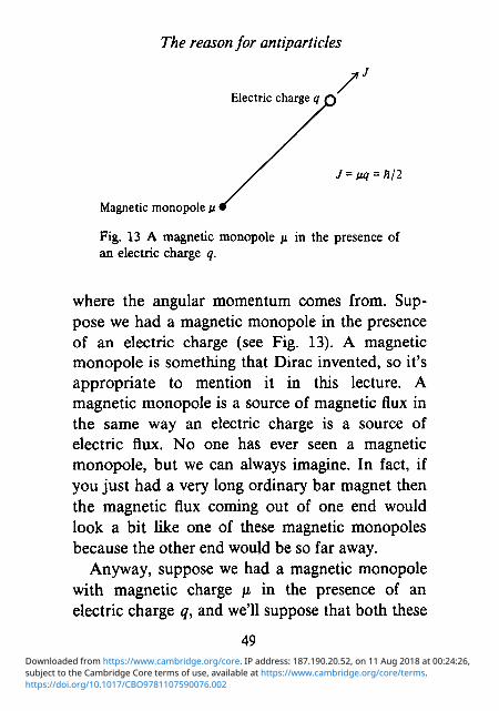
Fig. 13 A magnetic monopole ji in the presence of an electric charge q.

where the angular momentum comes from. Suppose we had a magnetic monopole in the presence of an electric charge (see Fig. 13). A magnetic monopole is something that Dirac invented, so it's appropriate to mention it in this lecture. A magnetic monopole is a source of magnetic flux in the same way an electric charge is a source of electric flux. No one has ever seen a magnetic monopole, but we can always imagine. In fact, if you just had a very long ordinary bar magnet then the magnetic flux coming out of one end would look a bit like one of these magnetic monopoles because the other end would be so far away.

Anyway, suppose we had a magnetic monopole with magnetic charge ju. in the presence of an electric charge q, and we'll suppose that both these

49


https://doi.org/10.1017/CBO9781107590076.002



RICHARD P. FEYNMAN

objects have spin-zero, so we don't have to worry about any intrinsic angular momentum. But these objects are in each other's presence, so you can form the Poynting vector E A B in the normal fashion. Integrating over the Poynting vector tells you what the momentum is, and, if you work it out, this composite object has an angular momentum (along the line joining the charge and pole) which is independent of how far apart the two objects are. You can work out what the angular momentum is in many ways, and I'll leave it as an exercise, but it turns out that the angular momentum is equal to nq*.

Now in quantum mechanics angular momentum must be quantized. In fact, one is only allowed to have angular momentum in multiples of (1/2)h, so let's take the smallest value allowed, that is let pq = (1/2) h, so we have constructed ourselves a spin \ object. Then we should find that rotating this object through 360° changes the phase by - 1 ; let's see if it does.

* Perhaps the most elementary fashion for determining the angular momentum is to find the torque that must be applied to slew the axis (the line joining q and /x) around at angular velocity u by moving the electron around a circle about the pole. The force, of course, comes from the motion of the electron in the magnetic field of the pole.

50


https://doi.org/10.1017/CBO9781107590076.002




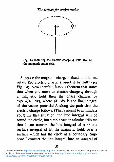
Fig. 14 Rotating the electric charge q 360° around the magnetic monopole.

Suppose the magnetic charge is fixed, and let me rotate the electric charge around it by 360° (see Fig. 14). Now there's a famous theorem that states that when you move an electric charge q through a magnetic field then the phase changes by exp(i^/A • dx), where /A • dx is the line integral of the vector potential A along the path that the electric charge follows. (That's meant to intimidate you!) In this situation, the line integral will be round the circle, but simple vector calculus tells me that I can convert the line integral of A into a surface integral of B, the magnetic field, over a surface which has the circle as a boundary. Suppose I convert the line integral into an integral of

51


https://doi.org/10.1017/CBO9781107590076.002



RICHARD P. FEYNMAN

B over the upper hemisphere. The surface integral of B is just the flux flowing through the surface. Now the total flux emitted by the magnetic mono-pole is 47771, i.e. the integral of the flux over an entire sphere which completely enclosed the mono-pole would be 47rju,. Here we're only integrating over a hemisphere so we get half this, namely 21771. Thus the total phase change will be exp(277iju )̂ and using nq = \, this works out as exp(i77-) = - 1 , no problem, it's absolutely right.

At this point I must digress briefly, because we are so close to an argument of Dirac's which shows that if just one monopole exists somewhere in the universe then electric charge must be quantized. The argument goes like this. Had I chosen to integrate over the lower hemisphere instead of the upper one, I would have gotten the same answer. In that case, the surface has the opposite orientation with respect to the direction of the line integral, so the phase change turns out to be exp(-i7r), which is still ( -1) . But notice that if the charge q were not quantized, at a multiple of h/2\i, then the two different surfaces would give different answers; an inconsistency. Hence the existence of magnetic monopoles implies charge quantization, and since we believe charge is

52


https://doi.org/10.1017/CBO9781107590076.002



A


\ X ^

AQ © £ \ y

(a)

X y \ © QB • • / i© © 5

\ \ \

V V ,

/ /

(b) (c)

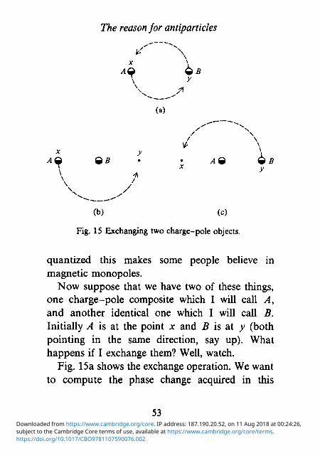
Fig. 15 Exchanging two charge-pole objects.

quantized this makes some people believe in magnetic monopoles.

Now suppose that we have two of these things, one charge-pole composite which I will call A, and another identical one which I will call B. Initially A is at the point x and B is at y (both pointing in the same direction, say up). What happens if I exchange them? Well, watch.

Fig. 15a shows the exchange operation. We want to compute the phase change acquired in this

53


https://doi.org/10.1017/CBO9781107590076.002



RICHARD P. FEYNMAN

process. The only sources of phase changes are from the change in A moving round the pole in B, and the change in B moving round the pole in A. (The relative positions of the charge and pole within each composite do not change.) As seen by B, the exchange operation looks like Fig. 15b, while to A it looks like Fig. 15 c. Each relative motion contributes to the total overall phase change an amount exp(i^/A • dx/h). Since A is moving 180° around B, and B itself is moving 180° around A, there is a 360° rotation here. Working out the phase change by looking at the line integrals, Fig. 15b gives a line integral from x to y, but Fig. 15c gives a line integral returning from y to Jt-putting the two together you get the line integral around a complete closed loop around a pole just as for a 360° rotation and hence a factor of ( — 1), as we have seen before. This is exactly what you expect with Fermi statistics of course-one has a factor of ( -1 ) when two spin \ objects are interchanged. (We assumed the spin-zero parts, charges and poles, obeyed Bose rules.)

SUMMARY

We've gone a long distance in great detail, but the basic ideas are the things to remember. Here's how

54


https://doi.org/10.1017/CBO9781107590076.002




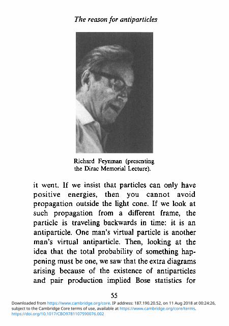
Richard Feynman (presenting the Dirac Memorial Lecture).

it went. If we insist that particles can only have positive energies, then you cannot avoid propagation outside the light cone. If we look at such propagation from a different frame, the particle is traveling backwards in time: it is an antiparticle. One man's virtual particle is another man's virtual antiparticle. Then, looking at the idea that the total probability of something happening must be one, we saw that the extra diagrams arising because of the existence of antiparticles and pair production implied Bose statistics for

55


https://doi.org/10.1017/CBO9781107590076.002



RICHARD P. FEYNMAN

spinless particles. When we tried the same idea on fermions, we saw that exchanging particles gave us a minus sign: they obey Fermi statistics. The general rule, was that a double time reversal is the same as a 360° rotation. This gave us the connection between spin and statistics and the Pauli exclusion principle for spin \. That contains everything, and the rest was just elaboration.

This is properly all that was in the lecture, but from talking with some of you and further thought, I should like to add some remarks that make the connection of spin and statistics still more obvious and direct. The discussion of the pole and charge objects obtained its result not through relativistic analysis of the action of two time reversals, but directly as the result of a 360° rotation. This argument can be made more general. We take the view that the Bose rule is obvious from some kind of understanding that the amplitude in quantum mechanics that correspond to alternatives must be added. What about the Fermi case?

We have noted that for half integral spin objects the sign of an amphtude might be obscure, for

56


https://doi.org/10.1017/CBO9781107590076.002




360° rotations may have occurred without having been noticed.

Now the spin-statistics rule that we wish to understand can be stated for both cases simultaneously by the following single rule: The effect on the wave function of the exchange of two particles is the same as the effect of rotating the frame of one of them by 360° relative to the other's frame. And why should this be true? Why, simply because such an exchange implies exactly such a relative frame rotation!

We have already noticed, in the pole-charge example, that if A and B are swapped (by paths that do not exactly intersect) A finds B going around it by a 180° rotation, and B sees A going around it also by 180° in the same direction; a mutual rotation by 360°.

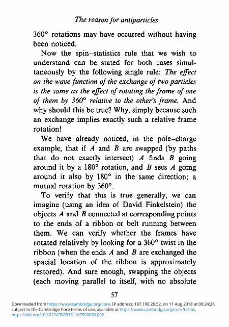
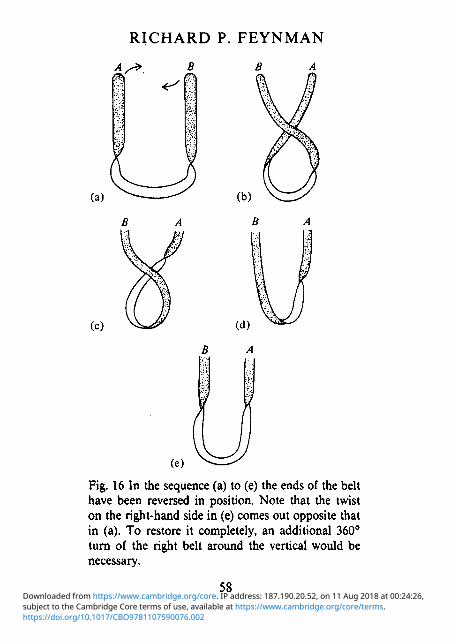
To verify that this is true generally, we can imagine (using an idea of David Finkelstein) the objects A and B connected at corresponding points to the ends of a ribbon or belt running between them. We can verify whether the frames have rotated relatively by looking for a 360° twist in the ribbon (when the ends A and B are exchanged the spacial location of the ribbon is approximately restored). And sure enough, swapping the objects (each moving parallel to itself, with no absolute

57


https://doi.org/10.1017/CBO9781107590076.002



RICHARD P. FEYNMAN

Fig. 16 In the sequence (a) to (e) the ends of the belt have been reversed in position. Note that the twist on the right-hand side in (e) conies out opposite that in (a). To restore it completely, an additional 360° turn of the right belt around the vertical would be necessary.

58


https://doi.org/10.1017/CBO9781107590076.002




rotation) induces exactly such a twist in the ribbon (see Fig. 16).

Since exchange implies such a 360° rotation of one object relative to the other, there is every reason to expect the (-1) phase factor occasioned by such a rotation for exchange of half integral spin objects.

59


https://doi.org/10.1017/CBO9781107590076.002




https://doi.org/10.1017/CBO9781107590076.002



Documents

FOR ANTIPARTICLES Richard P. Feynman The title of this ...alberto/apuntes/feynman.pdf · THE REASON FOR ANTIPARTICLES Richard P. Feynman The title of this lecture is somewhat incomplete