Int. J. Appl. Comput. MathDOI 10.1007/s40819-015-0106-y

ORIGINAL PAPER

Amplitude Equation and Heat Transportfor Rayleigh–Bénard Convection in Newtonian Liquidswith Nanoparticles

P. G. Siddheshwar1 · N. Meenakshi1

© Springer India Pvt. Ltd. 2015

Abstract Rayleigh–Bénard convection in liquids with nanoparticles is modelled as a singlephase systemwith liquid properties like density, viscosity, thermal expansion coefficient, heatcapacity and thermal conductivity modified by the presence of the nanoparticles. Expressionsfor the thermophysical properties are chosen from earlier works. The tri-modal Lorenzmodelis derived under the assumptions of Boussinesq approximation and small-scale convectivemotions. Ginzburg–Landau equation is arrived at from the generalized Lorenz model. Theamplitudes of convective modes required for estimating the heat transport are determinedanalytically. A table is prepared documenting the actual values of the thermophysical proper-ties of water, ethylene-glycol, engine-oil and glycerine with different nanoparticles, namelycopper, copper oxide, titania, silver and alumina, andNusselt number is calculated. Enhancedthermal conductivity being the reason for the enhancement of heat transport due to the pres-ence of the nanoparticles is shown. Detailed discussion is made on the percentage increaseof heat transport in twenty Newtonian nanoliquids compared to that in Newtonian liquidswithout nanoparticles.

Keywords Rayleigh–Bénard convection ·Heat transport ·Nanoliquids · Tri-modal Lorenzmodel · Ginzburg–Landau equation

Introduction

Nanoliquid comprises of a carrier liquid such as water or ethylene-glycol or engine-oil orglycerine with a dilute concentration of nanoparticles such as metallic or metallic oxideparticles (Cu, CuO, TiO2, Ag, Al2O3), having dimensions from 1 to 100 nm. It was Choi

B P. G. Siddheshwarmathdrpgs@gmail.com

N. Meenakshimeenakshi.nerolu@gmail.com

1 Department of Mathematics, Bangalore University, Jnanabharathi Campus,Bangalore 560 056, India

123

Int. J. Appl. Comput. Math

[10] who first proposed this term “Nanoliquid”. A significant feature of nanoliquids is ther-mal conductivity enhancement, a phenomenon which was first reported by Masuda et al.[29]. Eastman et al. [16] reported an increase of 40% in the effective thermal conductivityof ethylene-glycol with 0.3% volume of copper nanoparticles of 10nm diameter. Further10–30% increase of the effective thermal conductivity in alumina/water nanoliquids with1–4% of alumina was reported by Das et al. [12]. These reports led Buongiorno and Hu [8]to suggest the possibility of using nanoliquids in advanced nuclear systems.

A comprehensive review on thermal transport in nanoliquids was made by Eastman et al.[17] who concluded that despite several attempts, a satisfactory explanation for the abnor-mal enhancement in thermal conductivity and viscosity in nanoliquids is yet to be found.Buongiorno [7] conducted an extensive study of convective transport in nanoliquids butfocused on explaining the further heat transfer enhancements observed during convectivesituations. Ruling out dispersion, turbulence and particle rotation as significant agents forheat transfer enhancements, Buongiorno [7] suggested a new model based on the mechanicsof nanoparticles/carrier-liquid relative velocity. He observed that the absolute velocity ofnanoparticles can be taken as the sum total of the carrier-liquid velocity and a slip velocity.He considered seven slip mechanisms- inertia, Brownian diffusion, thermophoresis, diffu-sophoresis, Magnus effects, liquid drainage and gravity settling. He studied each one of theseand concluded that in the absence of turbulent effects, Brownian diffusion and thermophore-sis would dominate. Based on these two effects, he derived the conservation equations. Withthe help of the transport equations of Buongiorno [7], Tzou [36,37] studied the onset ofconvection in a horizontal layer of a nanoliquid heated uniformly from below and found thatas a result of Brownian motion and thermophoresis of nanoparticles, the critical Rayleighnumber was found to be much lower, by one to two orders of magnitude, than that of anordinary liquid. Kim et al. [26–28] also investigated the onset of convection in a hori-zontal nanoliquid layer and modified the three quantities, namely the thermal expansioncoefficient, the thermal diffusivity and the kinematic viscosity that appear in the defini-tion of the Rayleigh number. The role of thermophoresis in laminar natural convection in aRayleigh–Bénard cell filled with a water-based CuO nanoliquid was studied by Eslamian etal. [15].

Apart from the papers discussed above, there are other related works on this problem[4,13,14]. All the above works are based on the two-phase model with both the liquid andsolid phases playing a distinct role in the heat transfer process. Khanafer et al. [25] and Jouand Tzeng [24] have argued in favour of modelling nanoliquids as a single-phase model onthe reason that as of now there is no concrete theoretical ground on which enhanced heattransfer in nanoliquids can be explained. It thus becomes clear that in seeking to explainenhanced heat transfer, an alternate way of studying thermoconvective motion in nanoliquidsin the form a single-phase model can be quite naturally considered. In this model the liquidand solid phases are in local thermal equilibrium and flow with the same local velocity. Thissignifies that the nanoparticles and the liquid particles have similar properties so far as flow isconcerned but have different thermal properties. Thus in this model nanoliquid behaves moreas a liquid rather than as a solid–liquidmixture as in the conventional two-phasemodel. Sincein the single-phase model, properties of nanoliquids have contributions from the solid andliquid phases, the density, thermal expansion coefficient, specific heat, thermal conductivityof the two phases, viscosity of carrier liquid and nanoparticle concentration contribute to thenanoliquid properties. In addition, based on the experimental observation that heat transportis enhanced only when nanoparticle concentration is dilute, nanoparticle volume fraction hasto be assumed quite small. It needs to be emphasized here that this paper only estimates heattransport in nanoliquids using the single-phase model discussed in Khanafer et al. [25] and

123

Int. J. Appl. Comput. Math

Tiwari and Das [35]. Simo et al. [34] studied Rayleigh–Bénard convection in a cube withperfectly conducting lateral walls using the Galerkin spectral method. They analysed thestability properties and bifurcations of fixed point and also discussed about chaotic motions.The effect of nanoparticles on chaotic convection in a liquid layer heated from below wasstudied by Hashim et al. [23]. Corcione [11] in his paper on Rayleigh–Bénard convectionof nanoliquids assumed a single-phase model for nanoliquid. In this paper two empiricalequations are adopted from earlier works [11,25,35] for the evaluation of the effective valueof nanoliquid thermal conductivity and dynamic viscosity based on a wide variety of exper-imental data reported in the literature. The other effective properties are evaluated by thetraditional mixing theory. Park [31] investigated Rayleigh–Bénard convection of nanoliquidsusing a single-phase continuum model but with thermophysical properties assumed to bethat of nanoliquids rather than that of carrier liquids. The study predicts enhancement ofheat transfer. A good account of many aspects of enhanced heat transfer in nanoliquids isdiscussed in the books by Bianco et al. [5] and Bergman et al. [3]. In the absence of experi-mental works on heat transport in nanoliquids, it remains to be seen whether the single-phaseor the two-phase model is best suited as a mathematical model for natural convection innanoliquids.

Carrier liquids with a range of thermal conductivity from weakly thermally conductingto reasonably well conducting liquids has been chosen for investigation in combination withnanoparticles whose thermal conductivity ranges from very well conducting to extremelywell conducting solids. Such combinations gave rise to a wide spectrum of Prandtl numbersfor investigation. The above consideration led to the choice of the twenty nanoliquids chosenfor investigation in the paper. Curiosity as to whether high thermal conductivity in nanoparti-cles leads to high thermal conductivity in nanoliquids and thereby to enhanced heat transportin nanoliquids is the reason for our considering in the paper comparison of heat transportsin twenty nanoliquids. In the paper we study Rayleigh–Bénard convection in liquids withnanoparticles modelled as a single phase system with liquid properties like density, viscos-ity, thermal expansion coefficient, heat capacity and thermal conductivity modified by thepresence of the nanoparticles. Thermal convection in nanoliquids has mainly been studiedbetween two vertical plates with differential temperature or natural convection in nanoliq-uids due to a hot vertical plate. Natural convection in the Rayleigh–Bénard configuration hasbeen very less studied in most nanoliquids in enclosures. This is the reason why the classicalproblem of Rayleigh–Benard in nanoliquids has been undertaken in the current study.

Mathematical Formulation

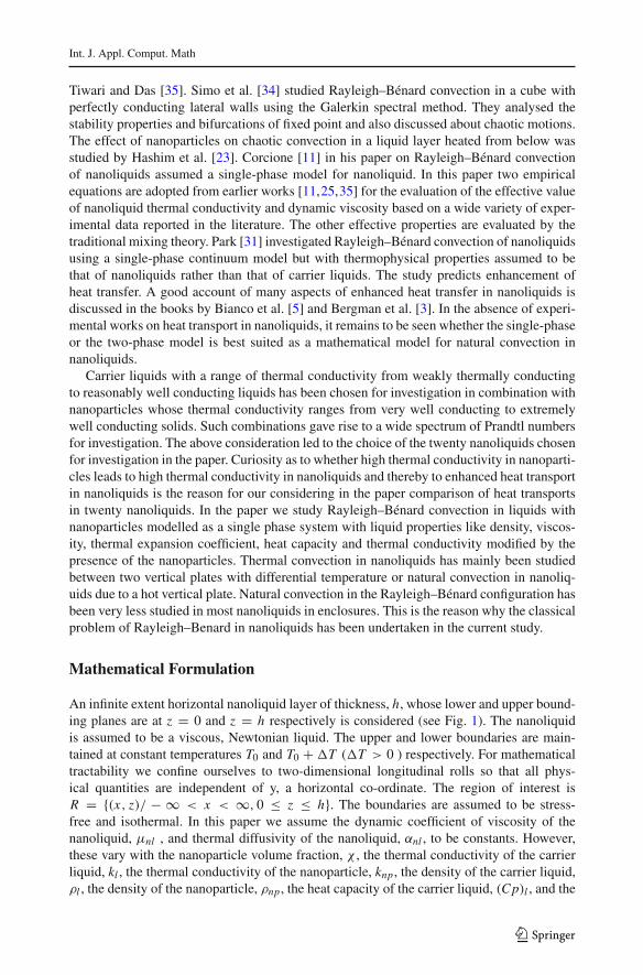
An infinite extent horizontal nanoliquid layer of thickness, h, whose lower and upper bound-ing planes are at z = 0 and z = h respectively is considered (see Fig. 1). The nanoliquidis assumed to be a viscous, Newtonian liquid. The upper and lower boundaries are main-tained at constant temperatures T0 and T0 + �T (�T > 0 ) respectively. For mathematicaltractability we confine ourselves to two-dimensional longitudinal rolls so that all phys-ical quantities are independent of y, a horizontal co-ordinate. The region of interest isR = {(x, z)/ − ∞ < x < ∞, 0 ≤ z ≤ h}. The boundaries are assumed to be stress-free and isothermal. In this paper we assume the dynamic coefficient of viscosity of thenanoliquid, μnl , and thermal diffusivity of the nanoliquid, αnl , to be constants. However,these vary with the nanoparticle volume fraction, χ , the thermal conductivity of the carrierliquid, kl , the thermal conductivity of the nanoparticle, knp , the density of the carrier liquid,ρl , the density of the nanoparticle, ρnp , the heat capacity of the carrier liquid, (Cp)l , and the

123

Int. J. Appl. Comput. Math

Fig. 1 Physical configuration

heat capacity of the nanoparticle, (Cp)np . We assume that the Oberbeck–Boussinesq approx-imation is valid and that there is thermal equilibrium between the Newtonian carrier liquidand the nanoparticles. The governing equations describing the Rayleigh–Bénard instabilitysituation in a Newtonian nanoliquid with constant viscosity are:Conservation of Mass

∇ · q = 0, (1)

Conservation of Momentum

ρnl

[∂q∂t

+ (q · ∇)q]

= −∇ p + μnl∇2q + [ρnl − (ρβ)nl (T − T0)

]g, (2)

Conservation of Energy

∂T

∂t+ (q · ∇)T = αnl∇2T, (3)

where the nanoliquid properties are obtained from either phenomenological laws or mixturetheory as given below [6,19]:

a. Phenomenological laws:

μnl

μl= 1

(1 − χ)2.5(Brinkman model) [6], (4)

knlkl

=

(knpkl

+ 2

)− 2χ

(1 − knp

kl

)(knpkl

+ 2

)+ χ

(1 − knp

kl

)

(Hamilton–Crosser model for stagnant conditions) [19] (5)

123

Int. J. Appl. Comput. Math

b. Mixture theory:

αnl = knl(ρCp)nl

ρnl

ρl= (1 − χ) + χ

ρnp

ρl(ρCp)nl

(ρCp)l= (1 − χ) + χ

(ρCp)np

(ρCp)l(ρβ)nl

(ρβ)l= (1 − χ) + χ

(ρβ)np

(ρβ)l

⎫⎪⎪⎪⎪⎪⎪⎪⎪⎪⎬⎪⎪⎪⎪⎪⎪⎪⎪⎪⎭

. (6)

In the Eqs. (1–6), q = (u, 0, w) is the velocity vector, u is horizontal component of velocity,w is vertical component of velocity, x is horizontal coordinate, z is vertical coordinate, ρnlis the density of the nanoliquid at T = T0, t is the time, p is the total pressure, μnl is thedynamic coefficient of viscosity of the nanoliquid, βnl is the coefficient of thermal expansionof the nanoliquid, T is the dimensional temperature, g = (0, 0,−g) is the acceleration dueto gravity, αnl is the thermal diffusivity of the nanoliquid, μl is the dynamic coefficient ofviscosity of the carrier liquid, knl is the thermal conductivity of the nanoliquid, (Cp)nl is theheat capacity of the nanoliquid, βl is the coefficient of thermal expansion of the carrier liquidand βnp is the coefficient of thermal expansion of the nanoparticle.The expression for effective viscosity and effective thermal conductivity is applicable forspherical-particles suspended in a carrier liquid. These models are discussed in detail byKhanafer et al. [25]. Taking the velocity, temperature and density fields in the quiescent basicstate to be qb(z) = (0, 0), Tb(z) and ρb(z), we obtain the quiescent state solution in the form:

qb = (0, 0)

Tb = T0 + �T f( zh

)pb = − ∫

ρb( zh

)gdz + C

⎫⎪⎪⎬⎪⎪⎭

, (7)

where f( zh

)=

(1 − z

h

)and C is the constant of integration. The quiescent basic state

is motionless and, in fact, the initial state of the system. On the quiescent basic state wesuperimpose perturbation in the form:

q = qb + q ′

T = Tb( zh

) + T ′

ρ = ρb( zh

) + ρ′

p = pb( zh

) + p′

⎫⎪⎪⎪⎪⎪⎬⎪⎪⎪⎪⎪⎭

, (8)

where the prime indicates a perturbed quantity. Since we consider only two-dimensionaldisturbances, we introduce stream function as follows:

u′ = −∂ψ ′

∂z, w′ = ∂ψ ′

∂x, (9)

where ψ is the dimensional stream function. These satisfy Eq. (1) in the perturbed state.Eliminating the pressure in Eq. (2), incorporating the quiescent state solution and non-dimensionalizing the resulting equations as well as Eq. (3) using the following definition

(X, Z) =( xh

,z

h

), τ = αl

h2t, Ψ = ψ ′

αl, Θ = T ′

�T, (10)

123

Int. J. Appl. Comput. Math

we obtain the dimensionless form of the vorticity and heat transport equations as follows :

1

Prnl

∂

∂τ(∇2Ψ ) = a1∇4Ψ + a21Rnl

∂Θ

∂X− 1

PrnlJ (Ψ,∇2Ψ ), (11)

∂Θ

∂τ= ∂Ψ

∂X+ a1∇2Θ − J (Ψ,Θ), (12)

where X is the non-dimensional horizontal coordinate, Z is the non-dimensional verticalcoordinate, τ is non-dimensional time, Ψ is the non-dimensional stream function, Θ non-dimensional temperature and

a1 =

⎡⎢⎢⎣1 −

3χ(1 − knp

kl

)(knpkl

+ 2

)+ χ

(1 − knp

kl

)⎤⎥⎥⎦

(1 − χ) + χ(ρCp)np

(ρCp)l

Prnl = μnl

ρnlαnl(nanoliquid Prandtl number)

Rnl = (ρβ)nl g�Th3

αnlμnl(nanoliquid Rayleigh number)

J (Ψ, . . .) =

∣∣∣∣∣∣∣

∂Ψ

∂X

∂Ψ

∂Z∂

∂X(. . .)

∂

∂Z(. . .)

∣∣∣∣∣∣∣

⎫⎪⎪⎪⎪⎪⎪⎪⎪⎪⎪⎪⎪⎪⎪⎪⎪⎪⎪⎪⎪⎪⎪⎪⎪⎬⎪⎪⎪⎪⎪⎪⎪⎪⎪⎪⎪⎪⎪⎪⎪⎪⎪⎪⎪⎪⎪⎪⎪⎪⎭

. (13)

Equations (11–12) are solved using the boundary/periodicity conditions

Ψ = ∂2

∂Z2

(∂Ψ

∂X

)= Θ = 0 at Z = 0, 1,

Ψ

(X ± 2π

πκc, Z

)= Ψ (X, Z), Θ

(X ± 2π

πκc, Z

)= Θ(X, Z), (14)

where πκc is the critical wave number. In the next section we discuss the linear stabilityanalysis of the system which is of great utility in the local nonlinear stability analysis to bediscussed further on.

Linear Stability Analysis

It can easily be proved that the principle of exchange of stabilities (PES) is valid in theproblem and hence we consider only the marginal stationary state. In order to make a linearstability analysis we consider the linear and steady-state version of Eqs. (11–12) and assumethe solutions to be periodic waves of the form [9]:

Ψ (X, Z) = Ψ0 sin(πκX) sin(π Z), (15)

Θ(X, Z) = Θ0 cos(πκX) sin(π Z), (16)

The quantitiesΨ0 andΘ0 are, respectively, amplitudes of the stream function and temperatureand πκ is the wave number. The normal mode solutions of Eqs. (15) and (16) satisfy theboundary conditions in Eq. (14). In Eqs. (15) and (16), πκ is the horizontal wave number.

123

Int. J. Appl. Comput. Math

Following standard procedure, we can obtain the expression for the critical Rayleighnumber in the form:

Rnlc = η61

π2κ2c

= 27π4

4, (17)

where the critical wave number πκc = 0.707π and η21 = π2(κ2c + 1) = 3π2

2 . The criticalRayleigh number, Rnlc, indicates transition from linear to nonlinear instability. More on thisis discussed further on in the section on “Results and Discussion”.

The linear theory predicts only the condition for the onset of convection and is silent aboutthe heat transport. We now embark on a weakly non-linear analysis by means of a truncatedrepresentation of Fourier series for streamfunction and temperature fields to find the effect ofvarious parameters on finite-amplitude convection and to know the amount of heat transfer.

Local Nonlinear Stability Analysis

The first effect of nonlinearity is to distort the temperature field through the interaction of Ψ

andΘ . The distortion of temperature field will correspond to a change in the horizontal mean,i.e., a component of the form sin(2π z) will be generated. Substituting a minimal doubleFourier series which describes the unsteady finite-amplitude convection in a Newtoniannanoliquid given by

Ψ (X, Z , τ ) =√2η21

π2κA1(τ ) sin(πκc X) sin(π Z), (18)

Θ(X, Z , τ ) = Rnlc

Rnlπ

[√2B1(τ ) cos(πκc X) sin(π Z) − C1(τ ) sin(2π Z)

], (19)

into Eqs. (11–12) and adopting the standard orthogonalization procedure for the Galerkinexpansion, the following nonlinear autonomous system (generalized tri-modal Lorenzmodel)of differential equations is obtained:

d A1

dτ1= a1Prnl [a1B1 − A1], (20)

dB1

dτ1= rnl A1 − a1B1 − A1C1, (21)

dC1

dτ1= −a1bC1 + A1B1, (22)

where

τ1 = η21τ, rnl = Rnl

Rnlc, b = 4π2

η21(23)

and A1, B1 are amplitudes in normal mode solution and C1 is the amplitude of convectivemode. It is well known in the problems as these that the trajectories of the solution of theLorenz model in phase-space remain within a bounded region. In the next section we showthat this trapping region is, in fact, a sphere for the current problem.

123

Int. J. Appl. Comput. Math

Trapping Region

Multiplying Eqs. (20) and (21) by A1 and B1 respectively, we get

A1d A1

dτ1= −a1Prnl A

21 + a21 Prnl A1B1, (24)

B1dB1

dτ1= rnl A1B1 − a1B

21 − A1B1C1. (25)

Adding Eqs. (24) and (25), we get

A1d A1

dτ1+ B1

dB1

dτ1= −a1Prnl A

21 − a1B

21 + A1B1

[a21 Prnl + rnl − C1

]. (26)

To get an equation of a sphere from Eqs. (22) and (26), wemultiply Eq. (22) by (C1−a21 Pr−rnl) and add the resulting equation to Eq. (26). This gives us

dE

dτ1= A1

d A1

dτ1+ B1

dB1

dτ1+ (C1 − a21 Prnl − rnl)

d

dτ1

(C1 − a21 Prnl − rnl

). (27)

Integrating the above equation, we get the trapping region in the form

E = 1

2

[A21 + B2

1 + (C1 − a21 Prnl − rnl)2] . (28)

The post-onset trajectories of the Lorenz system (20–22) enter and stay within a sphere withcenter (0, 0, a21 Prnl + rnl) and radius

√2 given by

A21 + B2

1 + (C1 − a21 Prnl − rnl)2 = (

√2)2. (29)

Noting that the Lorenz model is, in general, not analytically tractable we now move on toderive the analytically tractableGinzburg–Landau equation from the tri-modal Lorenzmodel.

Ginzburg–Landau Amplitude Equation from the Lorenz Model

From the Eqs. (20) and (21), B1 and C1 can be obtained in terms of A1 as:

B1 = 1

a1

[1

a1Prnl

d A1

dτ1+ A1

], (30)

C1 = 1

A1

[(rnl − 1)A1 −

(1

Prnla1+ 1

a1

)d A1

dτ1− 1

Prnla21

d2A1

dτ 21

]. (31)

Substituting Eqs. (30) and (31) in Eq. (22), we get a third order differential equation in A1.

Neglecting terms of the type

(d3A1

dτ 31

),

(d A1

dτ1

)2

,

(d A1

dτ1

)(d2A1

dτ 21

), and A1

(d2A1

dτ 21

), we

get the Ginzburg–Landau model in the form

d A1

dτ1=

(Prnl

1 + Prnl

)(1

b

)[a1b(rnl − 1)A1 − 1

a1A31

]. (32)

123

Int. J. Appl. Comput. Math

Equation (32) is a Bernoulli equation in A1 which can be solved using an initial conditionA(0) = A0 and the solution is given by

A1(τ1) =A0a1

√b(rnl − 1) exp

(Prnla1(rnl−1)τ1

1+Prnl

)√A20 exp

(2Prnla1(rnl−1)τ1

1+Prnl

)+ a21b(rnl − 1) − A2

0

. (33)

It is one of the intentions of the paper to study the pre-onset and post-onset critical points ofthe tri-modal Lorenz model. The same is discussed below.

Steady Finite Amplitude Convection

We note that the nonlinear system of autonomous differential equations (20–22) is notamenable to analytical treatment for the general time-dependent variables and it is to besolved by means of a numerical method. However, in the case of steady motions, theseequations can be solved in closed form.

The solution of the system (20–22) with left hand sides omitted is

(0, 0, 0), (±a1√b(rnl − 1),±√

b(rnl − 1), (rnl − 1)). (34)

These are the post-onset critical points of the dynamical system (20–22). The solutionA1 = B1 = C1 = 0 of the Lorenz model represents the state of no convection and non-zerovalues represent the convective state. Following standard procedure with the linear systemof autonomous differential equations, it can be easily shown that the only pre-onset criticalpoint is (0, 0, 0) which is a saddle point. In the next section we quantify the heat transport interms of the Nusselt number within a wave-length distance in the horizontal direction at thelower boundary.

Nano-Particle-Enhanced Heat Transport in a Newtonian Liquid

The horizontally-averaged Nusselt number, Nunl , for the stationary mode of convection (thepreferred mode in this problem) in a nanoliquid evaluated at the lower boundary z = 0 for asingle wave-length is given by

Nunl = Heat transport by conduction + Heat transport by convection

Heat transport by conduction. (35)

From Fourier law, we know that

Heat transport by conduction =[kl

∫ 2ππκc

0

dΘb

d ZdX

]Z=0

, (36)

Heat transport by convection =[knl

∫ 2ππκc

0

∂Θ

∂ZdX

]Z=0

, (37)

123

Int. J. Appl. Comput. Math

where Θb = Tb − T0�T

. Using Eqs. (36) and (37) in Eq. (35) and simplifying, we get

Nunl = 1 + knlkl

⎡⎢⎢⎣

∫ 2κc0

(∂Θ

∂Z

)dX

∫ 2κc0

(dΘb

d Z

)dX

⎤⎥⎥⎦

Z=0

. (38)

In the conduction state there will be equilibrium between the liquid and solid phases and thusthermal conductivity can be taken to be that of the liquid phase. In the convective state the

thermal conductivity of the nanoliquid is to be assumed. It is on this reason that the ratioknlkl

appears in the expression for the Nusselt number in Eq. (38).Substituting Eqs. (7) and (19) in Eq. (38) and completing the integration, we get

Nunl(τ1) = 1 + 2

rnl[a1a2]C1(τ1), (39)

where

a2 = (1 − χ) + χ(ρCp)np

(ρCp)l(40)

and C1(τ1) is obtained as follows. Substitutingd A1

dτ1and its derivative from Eq. (32) in Eq.

(31), we get C1 in terms of A1 as:

C1(τ1) = − 1

[1 + Prnl ]2[P1 + P2A

21 + P3A

41

], (41)

where

P1 = Prnl(rnl − 1)2, (42)

P2 = −[4[rnl − 1]Prnl + [1 + Prnl ]2

a21b

], (43)

P3 = 3Prnla41b

2. (44)

For steady, finite-amplitude convection, we get C1 in the form

C1 = rnl − 1. (45)

With this the expression (39) takes the form

Nunl(∞) = 1 + 2 [a1a2]

[1 − 1

rnl

]. (46)

With the necessary background for analysing the results prepared in the previous sections,in what follows we discuss the results obtained and make a few conclusions.

Results and Discussion

Rayleigh–Bénard convection in nanoliquids is usually studied using one of the following twomodels:

123

Int. J. Appl. Comput. Math

1. Buongiorno [7] two-phase model and2. Khanafer–Vafai–Lightstone [25] single-phase model.

There are good number of papers dealingwith convective heat transfer in nanoliquids usingBuongiorno [7] two-phase model. An alternative to studying heat transfer in nanoliquids isprovided by Khanafer–Vafai–Lightstone [25] single-phase model. The present paper uses thelatter model.

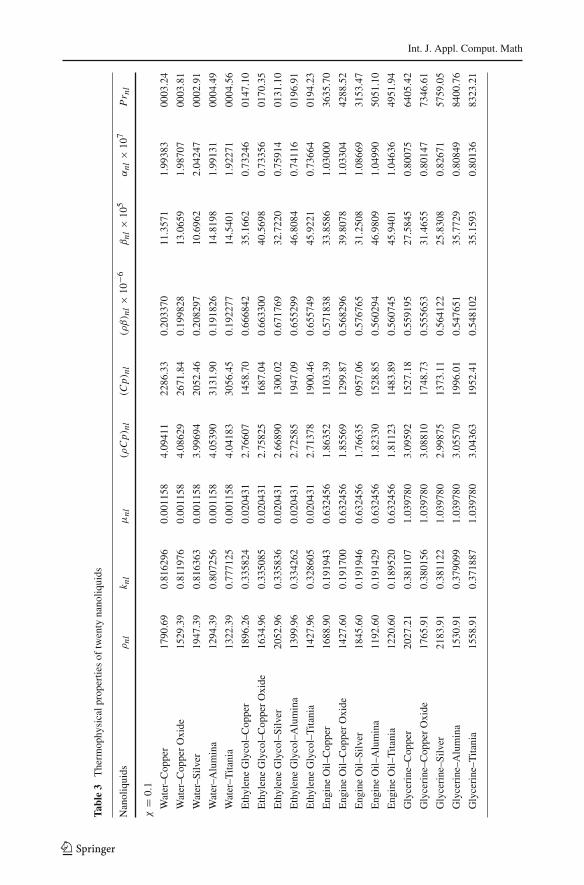
The definition of the nanoliquidRayleigh number as used in the paper is based on combinedproperties of the carrier liquid and the nanoparticles. To interpret the results in the case ofreal nanoliquids it becomes necessary to have information about the actual value of thethermophysical quantities of the carrier liquids and the nanoparticles under consideration inthe study. Tables 1 and 2 document information on the thermophysical quantities culled outfrom the papers of other investigators. Using the phenomenological laws and the mixturetheory, for calculating various thermophysical quantities of the nanoliquids as taken in Eqs.(4–6), and the values documented in Tables 1 and 2, the contents of Table 3 were arrived at.Also βnl and (Cp)nl were calculated using the following expressions:

βnl = (ρβ)nl

ρnl, (Cp)nl = (ρCp)nl

ρnl.

From Tables 1, 2 and 3 the following is apparent:

ρl < ρnl < ρnp, βl > βnl > βnp, Cpl > Cpnl > Cpnp and kl < knl � knp.

From the values of the above thermophysical quantities it is clear that the most significantchange in these quantities is seen for dilute concentrations and this is an experimentallyobserved fact as well. We use the above information in making the right conclusions from the

Table 1 Thermophysical properties of four carrier liquids at 300 ◦K

Quantity Pure water Ethylene glycol Engine oil Glycerine

Density (ρl ) [kg m3] 997.1 [18] 1114.4 [3] 884 [22] 1259.9 [3]

Thermal expansion coefficient (βl ) [K−1 × 105] 21 [18] 65 [3] 70 [22] 48 [3]

Specific heat (Cpl ) [J/kg − K] 4179 [18] 2415 [3] 1910 [22] 2427 [3]

Thermal conductivity (kl ) [W/m − K] 0.613 [18] 0.252 [3] 0.144 [22] 0.286 [3]

Dynamic viscosity (μl ) [kg/m − s] 0.00089 [21] 0.0157 [3] 0.486 [22] 0.799 [3]

Table 2 Thermophysical properties of five nanoparticles at 300 ◦K

Quantity Copper (Cu) Copper oxide (CuO) Silver (Ag) Alumina (Al2O3) Titania (TiO2)

Density (ρnp) [kg m3] 8933 [2] 6320 [18] 10500 [2] 3970 [2] 4250 [2]

Thermal expansioncoefficient (βnp)[K−1 × 105]

1.67 [2] 1.8 [18] 1.89 [2] 0.85 [2] 0.9 [2]

Specific heat (Cpnp)[J/kg − K]

385 [2] 531.8 [18] 235 [2] 765 [2] 686.2 [2]

Thermal conductivity(knp) [W/m − K]

401 [2] 76.5 [18] 429 [2] 40 [2] 8.9538 [2]

123

Int. J. Appl. Comput. Math

Table3

Therm

ophysicalp

ropertiesof

twenty

nanoliq

uids

Nanoliquids

ρnl

k nl

μnl

(ρCp)

nl(C

p)nl

(ρβ) nl×

10−6

βnl

×10

5αnl

×10

7Pr n

l

χ=

0.1

Water–C

opper

1790

.69

0.81

6296

0.00

1158

4.09

411

2286

.33

0.20

3370

11.357

11.99

383

0003

.24

Water–C

opperOxide

1529

.39

0.81

1976

0.00

1158

4.08

629

2671

.84

0.19

9828

13.065

91.98

707

0003

.81

Water–S

ilver

1947

.39

0.81

6363

0.00

1158

3.99

694

2052

.46

0.20

8297

10.696

22.04

247

0002

.91

Water–A

lumina

1294

.39

0.80

7256

0.00

1158

4.05

390

3131

.90

0.19

1826

14.819

81.99

131

0004

.49

Water–T

itania

1322

.39

0.77

7125

0.00

1158

4.04

183

3056

.45

0.19

2277

14.540

11.92

271

0004

.56

EthyleneGlycol–Cop

per

1896

.26

0.33

5824

0.02

0431

2.76

607

1458

.70

0.66

6842

35.166

20.73

246

0147

.10

EthyleneGlycol–Cop

perOxide

1634

.96

0.33

5085

0.02

0431

2.75

825

1687

.04

0.66

3300

40.569

80.73

356

0170

.35

EthyleneGlycol–Silver

2052

.96

0.33

5836

0.02

0431

2.66

890

1300

.02

0.67

1769

32.722

00.75

914

0131

.10

EthyleneGlycol–Alumina

1399

.96

0.33

4262

0.02

0431

2.72

585

1947

.09

0.65

5299

46.808

40.74

116

0196

.91

EthyleneGlycol–Tita

nia

1427

.96

0.32

8605

0.02

0431

2.71

378

1900

.46

0.65

5749

45.922

10.73

664

0194

.23

Eng

ineOil–

Cop

per

1688

.90

0.19

1943

0.63

2456

1.86

352

1103

.39

0.57

1838

33.858

61.03

000

3635

.70

Eng

ineOil–

Cop

perOxide

1427

.60

0.19

1700

0.63

2456

1.85

569

1299

.87

0.56

8296

39.807

81.03

304

4288

.52

Eng

ineOil–

Silver

1845

.60

0.19

1946

0.63

2456

1.76

635

0957

.06

0.57

6765

31.250

81.08

669

3153

.47

Eng

ineOil–

Alumina

1192

.60

0.19

1429

0.63

2456

1.82

330

1528

.85

0.56

0294

46.980

91.04

990

5051

.10

Eng

ineOil–

Tita

nia

1220

.60

0.18

9520

0.63

2456

1.81

123

1483

.89

0.56

0745

45.940

11.04

636

4951

.94

Glycerine–C

opper

2027

.21

0.38

1107

1.03

9780

3.09

592

1527

.18

0.55

9195

27.584

50.80

075

6405

.42

Glycerine–C

opperOxide

1765

.91

0.38

0156

1.03

9780

3.08

810

1748

.73

0.55

5653

31.465

50.80

147

7346

.61

Glycerine–S

ilver

2183

.91

0.38

1122

1.03

9780

2.99

875

1373

.11

0.56

4122

25.830

80.82

671

5759

.05

Glycerine–A

lumina

1530

.91

0.37

9099

1.03

9780

3.05

570

1996

.01

0.54

7651

35.772

90.80

849

8400

.76

Glycerine–T

itania

1558

.91

0.37

1887

1.03

9780

3.04

363

1952

.41

0.54

8102

35.159

30.80

136

8323

.21

123

Int. J. Appl. Comput. Math

Table 4 Values of the factor, F , for twenty nanoliquids

Nanoliquids χ = 0.06 χ = 0.1

F = (1−χ)2.5

a1(ρβ)nlρlβl

F = (1−χ)2.5

a1(ρβ)nlρlβl

Water–Copper 0.699739 0.550677

Water–Copper Oxide 0.693987 0.542925

Water–Silver 0.699719 0.550586

Water–Alumina 0.676852 0.520077

Water–Titania 0.692577 0.539897

Ethylene Glycol–Copper 0.696388 0.545479

Ethylene Glycol–Copper Oxide 0.693992 0.541769

Ethylene Glycol–Silver 0.684455 0.530194

Ethylene Glycol–Alumina 0.685280 0.529739

Ethylene Glycol–Titania 0.690936 0.533357

Engine Oil–Copper 0.729091 0.587987

Engine Oil–Copper Oxide 0.725130 0.582628

Engine Oil–Silver 0.708912 0.562118

Engine Oil–Alumina 0.712021 0.565198

Engine Oil–Titania 0.713823 0.567567

Glycerine–Copper 0.691894 0.539765

Glycerine–Copper Oxide 0.689356 0.535864

Glycerine–Silver 0.682258 0.527417

Glycerine–Alumina 0.680449 0.523562

Glycerine–Titania 0.687229 0.528650

result obtained on onset of convection. To understand the implication of the linear stabilityresults, one may rewrite Rnl as follows:

Rnl =[

(ρβ)nl

ρlβl

αl

αnl

μl

μnl

]Rl ,

where Rl = ρlβl g�Th3

μlαl. On computation, it is found that the factor, F, multiplying Rl

decreases with increase in χ . These results are shown in Table 4. From the above reasoningwe conclude that the critical nanoliquid Rayleigh number is less than that of the carrier liquidwithout nanoparticles, viz., Rlc. Thus, we may conclude that onset of convection is advancedby the addition of nanoparticles.

In what follows we discuss the results of a local nonlinear stability analysis of “LocalNonlinear Stability Analysis” section. For such an analysis the linear stability results areimportant. The critical point of the linear autonomous system is (0, 0, 0) which can only bea saddle point.

From Table 3 we note that except water-based nanoliquids all other nanoliquids have highPrandtl number, Prnl . In the context of the Lorenz model of Eqs. (20–22), Prnl >> 1 wouldmean the following:

123

Int. J. Appl. Comput. Math

B1 = A1

a1,

d A1

dτ1= a1[(rnl − 1)A1 − A1C1],

dC1

dτ1= A2

1

a1− a1bC1.

⎫⎪⎪⎪⎪⎪⎬⎪⎪⎪⎪⎪⎭

. (47)

In the system of Eq. 47, the second and third equations are solved for A1 and C1 and thenthe first equation is solved for B1.

The point (a1√b(rnl − 1),

√b(rnl − 1), rnl − 1) is the only critical point and hence the

trajectories are around this point (see Figs. 2, 3, 4, 5 and 6). In general, only one half of thebutterfly diagram normally seen in the case of the Lorenzmodel for Newtonian liquid withoutnanoparticles, can be realized in the case of the carrier liquids that we have considered herefor investigation. This is due to the fact that the Prandtl numbers of these liquids are quitelarge except for water which is 6.1.

Similar to the case of the classicalLorenzmodelwenote from theproceedings of “TrappingRegion” section that the trapping region of the post-onset trajectories of the Lorenz system isa sphere with center at (0, 0, a21 Prnl +rnl) and of radius

√2. From Eq. (47), it is evident that

in the absence of the nonlinear term and for rnl > 1, the amplitude A1 grows exponentially.

Fig. 2 Phase-plane trajectories in the AB, AC and BC planes respectively, for volume fraction, χ = 0.1,Prandtl number, Prnl = 4.55523, for water–titania nanoliquid

Fig. 3 Phase-plane trajectories in the AB, AC and BC planes respectively, for χ = 0.1, Prnl = 4.49345,for water–alumina nanoliquid

123

Int. J. Appl. Comput. Math

Fig. 4 Phase-plane trajectories in the AB, AC and BC planes respectively, for χ = 0.1, Prnl = 3.81111,for water–copper-oxide nanoliquid

Fig. 5 Phase-plane trajectories in the AB, AC and BC planes respectively, for χ = 0.1, Prnl = 3.24396,for water–copper nanoliquid

Fig. 6 Phase-plane trajectories in the AB, AC and BC planes respectively, for χ = 0.1, Prnl = 2.91189,for water–silver nanoliquid

123

Int. J. Appl. Comput. Math

We also know that the trajectories remain within the finiteness of a sphere (trappping region).These two observations clearly point to the fact that the nonlinear term A1C1 is responsiblefor altering the exponentially increasing nature of the trajectories and bringing it back to theconfines of a sphere.

In “Ginzburg–LandauAmplitudeEquation from theLorenzModel” section theGinzburg–Landau amplitude equation is derived from the Lorenz model. This result is important whenwe recognize the fact that Lorenzmodel is, in general, not analytically tractable butGinzburg–Landau equation is. This helps us in obtaining an analytical expression for the amplitudeand thereby the Nusselt number. We are mainly interested in quantifying heat transportin nanoliquids by steady finite-amplitude convection and also in analysing the essential

Fig. 7 The streamlines of unsteady convection at two different times for χ = 0.1, Prnl = 4.55523, forwater–titania nanoliquid. a τ1 = 0.05. b τ1 = 0.1

Fig. 8 The streamlines of unsteady convection at two different times for χ = 0.1, Prnl = 3153.47, forengine-oil–silver nanoliquid. a τ1 = 0.05. b τ1 = 0.1

123

Int. J. Appl. Comput. Math

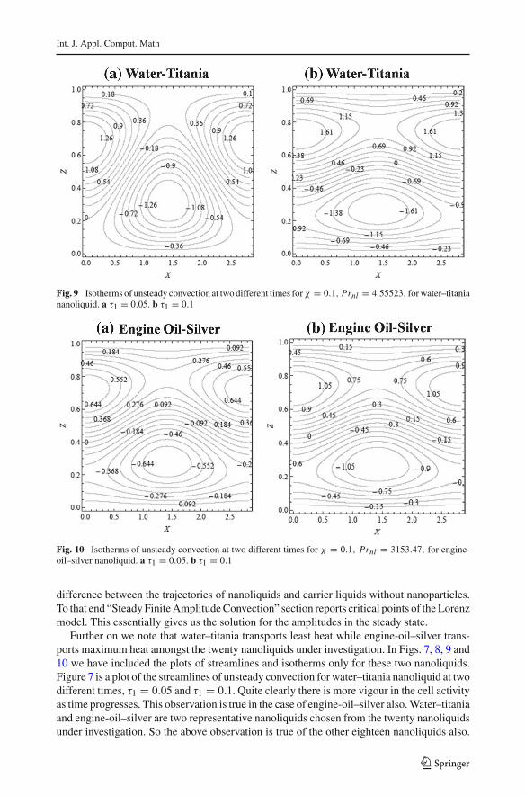
Fig. 9 Isotherms of unsteady convection at two different times forχ = 0.1, Prnl = 4.55523, forwater–titaniananoliquid. a τ1 = 0.05. b τ1 = 0.1

Fig. 10 Isotherms of unsteady convection at two different times for χ = 0.1, Prnl = 3153.47, for engine-oil–silver nanoliquid. a τ1 = 0.05. b τ1 = 0.1

difference between the trajectories of nanoliquids and carrier liquids without nanoparticles.To that end “Steady FiniteAmplitudeConvection” section reports critical points of the Lorenzmodel. This essentially gives us the solution for the amplitudes in the steady state.

Further on we note that water–titania transports least heat while engine-oil–silver trans-ports maximum heat amongst the twenty nanoliquids under investigation. In Figs. 7, 8, 9 and10 we have included the plots of streamlines and isotherms only for these two nanoliquids.Figure 7 is a plot of the streamlines of unsteady convection for water–titania nanoliquid at twodifferent times, τ1 = 0.05 and τ1 = 0.1. Quite clearly there is more vigour in the cell activityas time progresses. This observation is true in the case of engine-oil–silver also.Water–titaniaand engine-oil–silver are two representative nanoliquids chosen from the twenty nanoliquidsunder investigation. So the above observation is true of the other eighteen nanoliquids also.

123

Int. J. Appl. Comput. Math

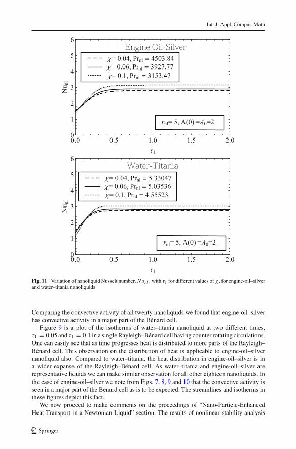
Fig. 11 Variation of nanoliquid Nusselt number, Nunl ,with τ1 for different values of χ , for engine-oil–silverand water–titania nanoliquids

Comparing the convective activity of all twenty nanoliquids we found that engine-oil–silverhas convective activity in a major part of the Bénard cell.

Figure 9 is a plot of the isotherms of water–titania nanoliquid at two different times,τ1 = 0.05 and τ1 = 0.1 in a single Rayleigh–Bénard cell having counter rotating circulations.One can easily see that as time progresses heat is distributed to more parts of the Rayleigh–Bénard cell. This observation on the distribution of heat is applicable to engine-oil–silvernanoliquid also. Compared to water–titania, the heat distribution in engine-oil–silver is ina wider expanse of the Rayleigh–Bénard cell. As water–titania and engine-oil–silver arerepresentative liquids we can make similar observation for all other eighteen nanoliquids. Inthe case of engine-oil–silver we note from Figs. 7, 8, 9 and 10 that the convective activity isseen in a major part of the Bénard cell as is to be expected. The streamlines and isotherms inthese figures depict this fact.

We now proceed to make comments on the proceedings of “Nano-Particle-EnhancedHeat Transport in a Newtonian Liquid” section. The results of nonlinear stability analysis

123

Int. J. Appl. Comput. Math

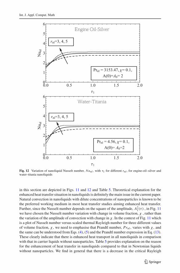
Fig. 12 Variation of nanoliquid Nusselt number, Nunl , with τ1 for different rnl , for engine-oil–silver andwater–titania nanoliquids

in this section are depicted in Figs. 11 and 12 and Table 5. Theoretical explanation for theenhanced heat transfer situation in nanoliquids is definitely themain issue in the current paper.Natural convection in nanoliquids with dilute concentrations of nanoparticles is known to bethe preferred working medium in most heat transfer studies aiming enhanced heat transfer.Further, since the Nusselt number depends on the square of the amplitude, A2

1(τ ) , in Fig. 11we have chosen the Nusselt number variation with change in volume fraction, χ , rather thanthe variation of the amplitude of convection with change in χ . In the context of Fig. 11 whichis a plot of Nusselt number versus scaled thermal Rayleigh number for three different valuesof volume fraction, χ, we need to emphasise that Prandtl number, Prnl , varies with χ, andthe same can be understood from Eqs. (4), (5) and the Prandtl number expression in Eq. (13).These clearly indicate that there is enhanced heat transport in all nanoliquids in comparisonwith that in carrier liquids without nanoparticles. Table 5 provides explanation on the reasonfor the enhancement of heat transfer in nanoliquids compared to that in Newtonian liquidswithout nanoparticles. We find in general that there is a decrease in the critical Rayleigh

123

Int. J. Appl. Comput. Math

Table 5 Values of nanoliquid Nusselt number, Nunl , in the steady state for χ = 0.1, Rnlc = 657.511, withNul = 2 for Rnl = 2Rnlc and Nul = 2.3333 for Rnl = 3Rnlc

Nanoliquids Nunl % increase in Nunl

2 × Rnlc 3 × Rnlc 2 × Rnlc 3 × Rnlc

(a) Water-based nanoliquids

Water–Titania 2.26774 2.69032 13.3870 15.29959

Water–Alumina 2.31689 2.75586 15.8445 18.10845

Water–Copper Oxide 2.32459 2.76612 16.2295 18.54817

Water–Copper 2.33164 2.77552 16.5820 18.95103

Water–Silver 2.33175 2.77567 16.5875 18.95746

(b) Glycerine-based nanoliquids

Glycerine–Titania 2.30030 2.73374 15.01500 17.16045

Glycerine–Alumina 2.32552 2.76736 16.27600 18.60131

Glycerine–Copper Oxide 2.32921 2.77229 16.46050 18.81260

Glycerine–Copper 2.33254 2.77672 16.62700 19.00246

Glycerine–Silver 2.33259 2.77679 16.62950 19.00546

(c) Ethylene Glycol-based nanoliquids

Ethylene Glycol–Titania 2.30399 2.73865 15.1995 17.37088

Ethylene Glycol–Alumina 2.32643 2.76858 16.3215 18.65360

Ethylene Glycol–Copper Oxide 2.32970 2.77293 16.4850 18.84008

Ethylene Glycol–Copper 2.33264 2.77685 16.6320 19.00808

Ethylene Glycol–Silver 2.33268 2.77691 16.6340 19.01060

(d) Engine Oil-based nanoliquids

Engine Oil–Titania 2.31611 2.75481 15.80550 18.06345

Engine Oil–Alumina 2.32937 2.77249 16.46850 18.82117

Engine Oil–Copper Oxide 2.33125 2.77500 16.56250 18.92874

Engine Oil–Copper 2.33293 2.77725 16.64650 19.02517

Engine Oil–Silver 2.33296 2.77728 16.64800 19.02646

number of nanoliquids with increase in χ and thereby increase in Nunl with increase in χ .Also, Nunl increases with increase in scaled thermal Rayleigh number, rnl (see Figs. 11,12). Enhanced thermal conductivity of nanoliquids is clearly the reason for enhanced heattransport [see also factor a1a2 which is greater than unity in the convective part of the Nusseltnumber expression (46)].

Conclusion

The following general conclusions can be made from the study:

1. Thermodynamically correct results have been obtained in the study and this lends cre-dence to the fact that the choice of expression for the thermophysical parameters ofnanoliquids is a correct choice. The values of the critical Rayleigh number and the Nus-selt number obtained in the study are to be treated as estimates at best. This observationis made considering the fact that the phenomenological laws used in the study are basedon static conditions. Corcione [11] has made a very apt comment on this aspect.

123

Int. J. Appl. Comput. Math

2. Rnanoparticlelc < Rno nanoparticle

lc for all values of parameters and for all twenty nanoliquids.Rlc refers to carrier liquid critical Rayleigh number and the phrase in the superscriptsrefer to the presence or absence of nanoparticles.

3. Due to high Prandtl number in most nanoliquids considered in the study only one halfof the butterfly diagram can be obtained as the trajectory of the solution of the Lorenzmodel. This is unlike the case of carrier liquids without nanoparticles.

4. Convective activity in the case of nanoliquids is seen in regions quite interior to the cell.This is much more than what is seen in the case of carrier liquids without nanoparticles.

5. Amongst the twenty nanoliquids considered, it is found, in general, that engine-oil–silverhas the most enhanced heat transport while water–titania has the least. However, allnanoliquids transport more heat compared to a Newtonian liquid without nanoparticles.Thus the following is true:Nunl > Nul .

6. Enhanced thermal conductivity in nanoliquids is the reason for enhanced heat transport.7. Most experimental investigations [1,20,30,32,33] on natural convection in nanoliquids

do not pertain to a Rayleigh–Bénard set-up. In the absence of experimental works on heattransport in nanoliquids by Rayleigh–Bénard convection, it remains to be seen whetherthe single-phase or the two-phase model is best suited as a mathematical model forstudying heat transfer in nanoliquids.

Acknowledgments One of us (MN) is grateful to the Department of Science and Technology, Governmentof India, for awarding a junior research fellowship to carry out her research under the “Promotion forUniversityResearch and Scientific Excellence (PURSE)” programme. She is also grateful to the Bangalore Universityfor supporting her research. The authors are grateful to the two anonymous referees for their most usefulcomments that helped them refine the paper to the present form.

References

1. Abu-Nada, E.: Effects of variable viscosity and thermal conductivity of Al2O3 water nanofluid on heattransfer enhancement in natural convection. Int. J. Heat Fluid Flow 30, 679–690 (2009)

2. Abu-Nada, E., Masoud, Z., Hijazi, A.: Natural convection heat transfer enhancement in horizontal con-centric annuli using nanofluids. Int. Comm. Heat Mass Transfer 35, 567–665 (2008)

3. Bergman, T.L., Lavine, A.S., Incropera, F.P., Dewitt, D.P.: Fundamentals of Heat and Mass Transfer.Wiley, New York (2006)

4. Bhadauria, B.S., Agarwal, S.: Convective heat transport by longitudinal rolls in dilute nanoliquids. J.Nanofluids 3, 380–390 (2014)

5. Bianco, V., Manca, O., Nardini, S., Vafai, K.: Heat transfer enhancement with nanofluids. CRC Press,Canada (2015)

6. Brinkman, H.C.: The viscosity of concentrated suspensions and solutions. J. Chem. Phys. 20, 571–571(1952)

7. Buongiorno, J.: Convective transport in nanofluids. ASME J. Heat Transfer 128, 240–250 (2006)8. Buongiorno, J., Hu, W.: In: Proceedings of International Congress on Advances in Nuclear Power Plants:

ICAPP 05; May 15-19, Seoul, Korea, pp 3581–3585 (2005)9. Chandrasekhar, S.: Hydrodynamic andHydromagnetic Stability. Oxford University Press, London (1961)

10. Choi, S.U.S.: Enhancing thermal conductivity of fluids with nanoparticles. In: Siginer, D.A„ Wang, H.P.,(eds.) Developments and Applications of Non-Newtonian Flows. ASME; FED-231/MD66, pp 99–105(1995)

11. Corcione, M.: Rayleigh–Bénard convection heat transfer in nanoparticle suspensions. Int. J. Heat FluidFlow 32, 65–77 (2011)

12. Das, S.K., Putra, N., Thiesen, P., Roetzel, W.: Temperature dependence of thermal conductivity enhance-ment for nanofluids. ASME J. Heat Transfer 125, 567–574 (2003)

13. Dhananjaya, Y., Agrawal, G.S., Bhargava, R.: Rayleigh–Bénard convection in nanofluid. Int. J. Appl.Math. and Mech. 7(2), 61–76 (2011)

123

Int. J. Appl. Comput. Math

14. Dhananjaya, Y., Agrawal, G.S., Bhargava, R.: Thermal instability of rotating nanofluid layer. Int. J. Eng.Sci. 49, 1171–1184 (2011)

15. Eslamian,M., Ahmed,M., El-Dosoky,M.F., Saghir, M.Z.: Effect of thermophoresis on natural convectionin a Rayleigh–Bénard cell filled with a nanofluid. Int. J. Heat Mass Transfer 81, 142–156 (2015)

16. Eastman, J.A., Choi, S.U.S., Li, S., Yu, W., Thompson, L.J.: Anomalously increased effective thermalconductivities of ethylene glycol-based nanofluids containing copper nanoparticles. Appl. Phys. Lett. 78,718–720 (2001)

17. Eastman, J.A., Choi, S.U.S., Phillpot, S.R., Keblinski, P.: Thermal transport in nanofluids. Ann. Rev.Mater. Res. 34, 219–246 (2004)

18. Ghasemi, B., Aminosadati, S.M.: Natural convection heat transfer in an inclined enclosure filled with aWater-CuO nanofluid. Num. Heat Transfer 55, 807–823 (2009)

19. Hamilton, R.L., Crosser, O.K.: Thermal conductivity of heterogeneous two-component systems. Ind. Eng.Chem. Fund. 1, 187–191 (1962)

20. Ho, C.J., Chen, M.W., Li, Z.W.: Numerical simulation of natural convection of nanofluid in a squareenclosure: effects due to uncertainties of viscosity and thermal conductivity. Int. J. Heat Mass Transfer51, 4506–4516 (2008)

21. http://www.thermexcel.com/english/tables/eau_atm.htm22. http://www.thermalfluidscentral.org/encyclopedia/index.php23. Jawdat, J.M., Hashim, I., Momani, S.: Dynamical system analysis of thermal convection in a horizontal

layer of nanofluids heated from below. Math. Probl. Eng. 2012, 1–13 (2012)24. Jou, R.Y., Tzeng, S.C.: Numerical research on nature convective heat transfer enhancement filled with

nanofluids in rectangular enclosures. Int. Commun. Heat Mass Transfer 33, 727–736 (2006)25. Khanafer, K., Vafai, K., Lightstone,M.: Buoyancy driven heat transfer enhancement in a two-dimensional

enclosure utilizing nanofluids. Int. J. Heat Mass Transfer 46, 3639–3653 (2003)26. Kim, J., Kang, Y.T., Choi, C.K.: Analysis of convective instability and heat transfer characteristics of

nanofluids. Phys. Fluids 16, 2395–2401 (2004)27. Kim, J., Choi, C.K., Kang, Y.T., Kim, M.G.: Effects of thermodiffusion and nanoparticles on convective

instabilities in binary nanofluids. Nanoscale Microscale Thermophys. Eng. 10, 29–39 (2006)28. Kim, J., Kang, Y.T., Choi, C.K.: Analysis of convective instability and heat transfer characteristics of

nanofluids. Int. J. Refrig. 30, 323–328 (2007)29. Masuda, H., Ebata, A., Teramae, K., Hishinuma, N.: Alteration of thermal conductivity and viscosity of

liquid by dispersing ultra fine particle. Netsu Bussei 7, 227–233 (1993)30. Oztop, H.F., Abu-Nada, E.: Numerical study of natural convection in partially heated rectangular enclo-

sures filled with nanofluids. Int. J. Heat Fluid Flow 29, 1326–1336 (2008)31. Park, H.M.: Rayleigh–Bénard convection of nanofluids based on the pseudo-single-phase continuum

model. Int. J. Therm. Sci. 90, 267–278 (2015)32. Polidori, G., Fohannoa, S., Nguyenb, C.T.: A note on heat transfer modelling of Newtonian nanofluids in

laminar free convection. Int. J. Therm. Sci. 46, 739–744 (2007)33. Putra, N., Roetzel, W., Das, S.K.: Natural convection of nano-fluids. Heat Mass Transfer 39, 775–784

(2003)34. Simo, C., Puigjaner, D., Herrero, J., Giralt, F.: Dynamics of particle trajectories in a Rayleigh–Bénard

problem. Commun. Nonlin. Sci. Numer. Simulat. 15, 24–39 (2010)35. Tiwari, R.K., Das, M.K.: Heat transfer augmentation in a two-sided lid-driven differentially heated square

cavity utilizing nanofluids. Int. J. Heat Mass Transfer 50, 2002–2018 (2007)36. Tzou, D.Y.: Instability of nanofluids in natural convection. ASME J. Heat Transfer 130(7), 1–9 (2008)37. Tzou, D.Y.: Thermal instability of nanofluids in natural convection. Int. J. Heat Mass Transfer 51, 2967–

2979 (2008)

123