For Richer or Poorer: Women, Men and Marriage

Janeen Baxter* and Edith Gray#

Negotiating the Life Course Discussion Paper Series Discussion Paper DP-012

April 2003

* Sociology, School of Social Science, The University of Queensland

# Centre for Social Research, Australian National University

Paper presented to 8th Australian Institute of Family Studies Conference. Melbourne 12-14 February, 2003.

2

Abstract In 1972 Jessie Bernard argued that women fared much worse in marriage than men. She

suggested that in every marriage there are two marriages “his” and “hers” and his is much

better than hers on almost every indicator—demographically, socially, and

psychologically. Almost three decades later the issues raised by Bernard are still being

debated. Waite and Gallagher (2000) have argued that all married people are happier,

healthier and better off financially than unmarried people. Most recently, DeVaus (2002)

claims that marriage reduces the risk of mental disorders for both men and women. Our

paper addresses these issues. Using data from the Negotiating the Life Course survey we

examine the relationship between marriage, gender and a range of social outcomes. We

focus on two main areas—outcomes associated with the labor market and outcomes

associated with the household. In particular we advance debates in the areas by

examining the experience of de facto cohabitations separately from legal marriage. This

enables us to examine the impact of the institutional status of marriage on outcomes as

opposed to cohabitation more generally.

3

Background

In 1972, Jessie Bernard argued in her well-known and influential book The Future of

Marriage, that “there are two marriages … in every marital union, his and hers. And his

… is better than hers.” (1982 Edition: 14) In support of this argument, Bernard pointed to

men’s power over women within marriage, women’s responsibility for unpaid household

labour, improved mortality and health rates for married men compared to unmarried men,

and higher reported levels of happiness and mental wellbeing for married men compared

to both unmarried men and married women (Bernard, 1972). In contrast, although on

some indicators of health, married women also fare better than single women, compared

to married men the benefits of marriage for women are far less. More wives than

husbands report negative feelings about their marriage, consider their marriages unhappy

and have considered separation or divorce, and moreover, wives have much poorer

mental and emotional health compared to husbands and to unmarried women (Bernard

1972).

Bernard considers the possibility that these findings may be due to sex differences

between men and women, that is, that women may be more prone to depression and

psychological distress than men. But she dismisses this argument by showing that the

mental and emotional health of women prior to marriage is as good as or better than that

for men suggesting that it is something about the marriage process itself that leads to

women’s poorer health. Additionally she considers the argument that selection effects

might explain the marriage differential, with certain kinds of men and women being

selected into marriage. Although, as Bernard notes, it is virtually impossible in the

absence of clinical experiments to rule out selectivity effects completely, she argues that

it is unlikely that they play a large role. It may be true that healthier men are more likely

to be selected into marriage than unhealthy men and this may account for some of the

health benefits observed for married men. But most people marry at some stage in their

lives, at least at the time that Bernard was writing. And the explanation does not work for

women since it is unlikely that men would choose to marry women who are unhappy,

depressed or psychologically distressed. Rather we would expect that women with these

characteristics would be selected out of marriage.

4

Almost thirty years later, Bernard’s argument has been challenged by a leading

American demographer, Linda Waite. In recent work Waite and Gallagher have argued

that:

Overall, the portrait of marriage that emerges from two generations of increasingly sophisticated empirical research on actual husbands and wives is not one of gender bias, but gender balance. A good marriage enlarges and enriches the lives of both men and women (2000: 163)

Waite and Gallagher acknowledge the evidence cited by Bernard in support of

differences in depression rates for married men and women, but argue that women are

simply more prone to depression than men. Moreover, they suggest that when broader

measures of mental health are used, there are no differences in rates of mental wellbeing

between married men and women (2000: 164). At the same time, they argue that the

cumulative results of a range of recent work that specifically examines depression, rather

than overall mental health, shows that marriage does not account for the depression gap

between men and women. On the contrary, marriage has a positive effect on women’s

levels of depression. Married people are less depressed and emotionally healthier than

comparable singles (2000: 166).

And they suggest that the reason the benefits in married men’s physical health are

so great compared to single men is because single men are far more likely to lead

unhealthy and antisocial lives compared to married men. On the other hand, single

women do not lead considerably more unhealthy lives than married women. “In other

words, the reason getting a wife boosts your health more than acquiring a husband is not

that marriage warps women, but that single men lead such warped lives” (2000: 164).

Waite and Gallagher also argue that Bernard’s work fails to distinguish between

the effects of marriage and children. While it is the case that in the time that Bernard was

writing, (the sixties), marriage was nearly always accompanied by children, Waite and

Gallagher argue that, “later work that controls for the presence of children finds that

marriage protects mothers from depression” (2000: 165). So while they acknowledge that

women with preschoolers report higher levels of stress and depression than women

without young children, and are more likely to report feeling a “time crunch” than their

5

childfree counterparts, they argue that the impact of marriage and mothering need to be

considered separately (2000: 164-165).

Consideration of the debate about whether marriage is good for men and women,

as posed by Bernard, and more recently Waite and Gallagher (and others such as De

Vaus, 2002), raises a number of issues that need to be considered. The apparently

straightforward comparison of the effects of marriage on men and women is more

complex than it might first appear. First it is undoubtedly the case that much has changed

since Bernard presented her argument in the early 1970s. Not only have the

demographics of marital formation and dissolution changed dramatically over this period,

with ages at first marriage rising significantly, fertility rates declining sharply, divorce

rates remaining significantly higher than in the 1960s and rates of pre-marital

cohabitation rising considerably, but also attitudes toward marriage have altered

markedly. Giddens (2001:17) has gone so far as to refer to these changes as a “global

revolution” in how we think of ourselves and how we form relationships with others.

Other commentators have made similar arguments (Beck and Beck-Gernsheim, 1995;

Beck-Gernsheim, 2002). At the same time, dramatic changes have taken place in

participation rates in higher education for both men and women, but particularly for

women, and married women have moved into and remained in paid employment in

greater numbers than ever before. Given these changes it may be that the patterns

observed by Bernard in the 1960s will be quite different to those observed by researchers

today.

Second it is important to clarify whether the comparison in the debate is across

marital status, that is comparing married and unmarried individuals, or is across gender,

that is comparing men and women. The results of these different comparisons may

suggest different conclusions. For example, married women may have better rates of

health than single women suggesting that marriage is good for women’s health. On the

other hand, married women may have poorer rates of health than married men,

suggesting that marriage is not good for women’s health. Further analyses would then be

needed to determine if marriage has had a bigger positive effect on men’s health than

women’s health, or whether men are just healthier than women regardless of marital

status.

6

Third, the conclusions reached will undoubtedly vary depending on the outcome

under consideration. In terms of responsibility for housework and unpaid caring work, the

evidence seems overwhelmingly clear that marriage is good for men and bad for women.

But other indicators may not be so clear-cut. While marriage may be bad for women in

terms of participation in paid employment and individual returns to wages, it may be

good for women in terms of providing access to a higher standard of living as a result of

access to husband’s income.

In the current paper we investigate the marriage debate using data from the

Negotiating the Life Course Project. The data collected as part of this project is

particularly useful for examining the debate as it contains detailed information on marital

history and relationships. It also contains information on a range of possible indicators for

examining the effects of marriage on men and women, including the domestic division of

labour, employment participation, earnings, health, wellbeing and attitudes. Our aim is to

contribute to this debate by using recent empirical data to assess the benefits of marriage

for men and women.

Further we hope to advance the debate by focusing on the experience of de facto

cohabitation as well as legal marriage. The percentage of couples cohabiting prior to

marriage has more than tripled in recent years. In 1976, 16% of couples cohabited prior

to marriage, but by 1992 this figure had jumped to 56% (De Vaus and Wolcott, 1997). By

examining the experiences of men and women within de facto relationships we hope to

be able to contribute to understandings of the institutional status of marriage as opposed

to partnerships more generally. For example, are the patterns observed by Bernard and

Waite and Gallagher apparent when comparing single people with those in de facto

relationships, suggesting that the key issue is cohabitation, or are they only apparent

when comparing single people with married people, suggesting that the key issue is

marriage?

In this paper we focus on three key areas: the relationship between marriage and

employment, marriage and earnings, and, marriage and housework.

7

The Negotiating the Life Course Project

The data used in this paper come from a 1996/97 national Australian survey titled

“Negotiating the Life Course: Gender, Mobility and Career Trajectories” (NLC). The

sample comprised 2,231 respondents between the ages of 18 and 54 randomly selected

from listed telephone numbers in the electronic white pages. Each respondent was

randomly selected from all 18 to 54 year olds in the household. The data were collected

using computer assisted telephone interviewing (CATI), with a response rate of 55%.

Details of the project can be obtained at http://lifecourse.anu.edu.au

Experiences in the labour force: Does marriage matter?

It has been previously found that there are many beneficial effects of marriage on men’s

careers. Men who are married do substantially better in the labour market, particularly in

terms of earnings, than men who are not married, but this is not the case for women (see

for example Richardson, 2000; Korenman and Neumark, 1991; Korenman and Neumark,

1992, Waldfogel, 1997). In Western countries it has been found that for women,

differential employment and career costs are due to childrearing. It is argued that it is not

marriage itself that explains women’s experience in the labour force, but the presence of

children. Children have an effect on both the differential employment of men and women

(Waldfogel, 1997; Gornick, 1999), but also on women’s longer term earning power

(Davies, Joshi and Peronaci, 2000). This is through both a loss of workplace experience,

and a lowering in the value of labour market skills (Chapman, et al. 2001). Further, for

mothers, educational background is also a key factor in explaining labour force

involvement (Desai and Waite, 1991; McLaughlin, 1982; Gray and McDonald, 2002).

This section compares the experiences of men and women in the labour force,

based on their marital status. This is part of the unpacking of the meaning and benefits (or

otherwise) of marriage (as suggested by Bachrach, Hindin and Thomson, 2000). The

analysis compares respondents from the NLC who are single, cohabiting or legally

married. The labour force experiences that are examined include: employment status;

number of hours spent in paid work per week; permanency; sector; and managerial level.

8

The analysis of each labour force experience is conducted for men and women and is

controlled by age, education level and child status. Predicted probabilities have been

calculated showing differences by relationship status for each labour force factor

(controlling for influences outlined).

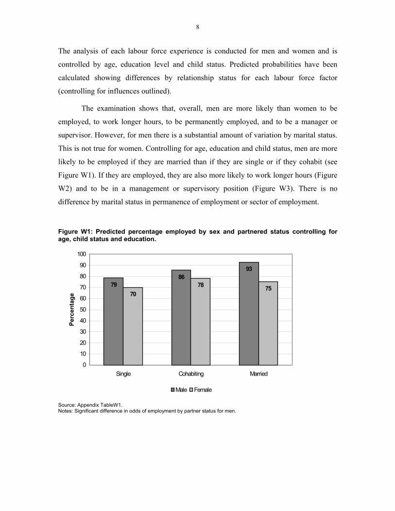
The examination shows that, overall, men are more likely than women to be

employed, to work longer hours, to be permanently employed, and to be a manager or

supervisor. However, for men there is a substantial amount of variation by marital status.

This is not true for women. Controlling for age, education and child status, men are more

likely to be employed if they are married than if they are single or if they cohabit (see

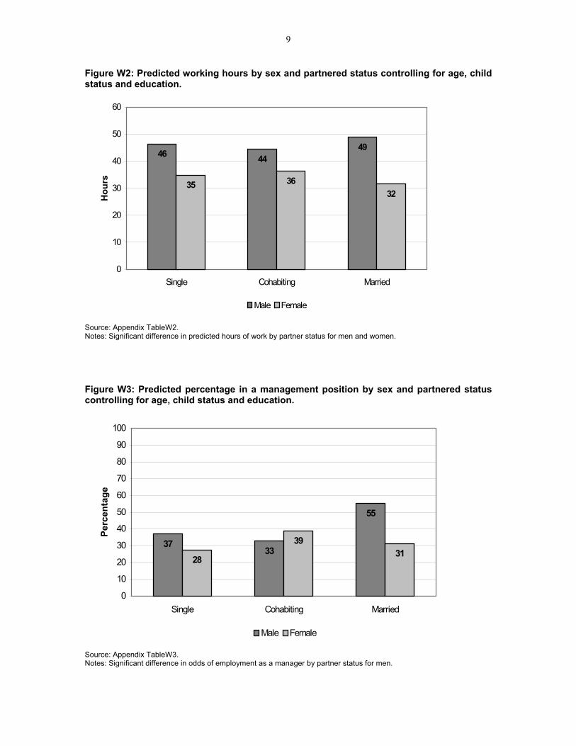
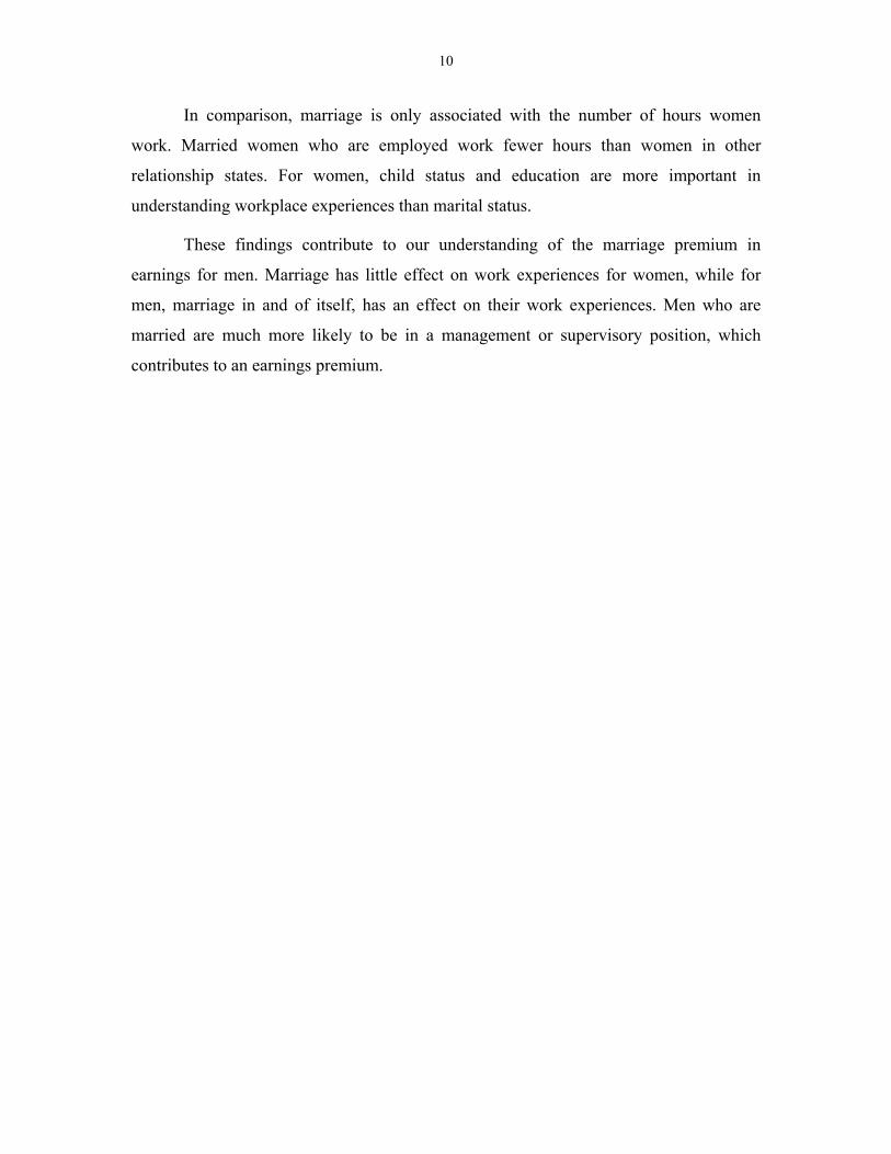
Figure W1). If they are employed, they are also more likely to work longer hours (Figure

W2) and to be in a management or supervisory position (Figure W3). There is no

difference by marital status in permanence of employment or sector of employment.

Figure W1: Predicted percentage employed by sex and partnered status controlling for age, child status and education.

7986

93

7078 75

0

10

20

30

40

50

60

70

80

90

100

Single Cohabiting Married

Perc

enta

ge

Male Female

Source: Appendix TableW1. Notes: Significant difference in odds of employment by partner status for men.

9

Figure W2: Predicted working hours by sex and partnered status controlling for age, child status and education.

46 4449

35 3632

0

10

20

30

40

50

60

Single Cohabiting Married

Hou

rs

Male Female

Source: Appendix TableW2. Notes: Significant difference in predicted hours of work by partner status for men and women. Figure W3: Predicted percentage in a management position by sex and partnered status controlling for age, child status and education.

3733

55

28

3931

0

10

20

30

40

50

60

70

80

90

100

Single Cohabiting Married

Perc

enta

ge

Male Female

Source: Appendix TableW3. Notes: Significant difference in odds of employment as a manager by partner status for men.

10

In comparison, marriage is only associated with the number of hours women

work. Married women who are employed work fewer hours than women in other

relationship states. For women, child status and education are more important in

understanding workplace experiences than marital status.

These findings contribute to our understanding of the marriage premium in

earnings for men. Marriage has little effect on work experiences for women, while for

men, marriage in and of itself, has an effect on their work experiences. Men who are

married are much more likely to be in a management or supervisory position, which

contributes to an earnings premium.

11

The Marriage Premium for Earnings1

A considerable amount of research has documented a marriage premium in earnings for

married men (Blackburn and Korenman, 1994; Dolton and Makepeace, 1987; Ginther

and Zarovdy, 2001; Gray, 1997; Hill, 1979; Korenman and Neumark, 1991; Korenman

and Neumark, 1992). The research suggests that marriage increases men’s earnings

potential for two main reasons. First because married men are more productive in

employment after marriage, largely as a result of the unpaid labour performed by women

in the home, which frees men to dedicate themselves to employment. Second, it has been

suggested that certain kinds of men are selected in to marriage and typically these will be

men who have higher earnings potential. While evidence has been found for both

explanations, on balance, the available research tends to favour the specialisation

argument where the gender division of labor in the household allows men the time and

energy to pursue labor market goals (Becker, 1985; Blackburn and Korenman, 1994;

Chalmers, 2002; Gray, 1997; Korenman and Neumark, 1991; Loh, 1996).

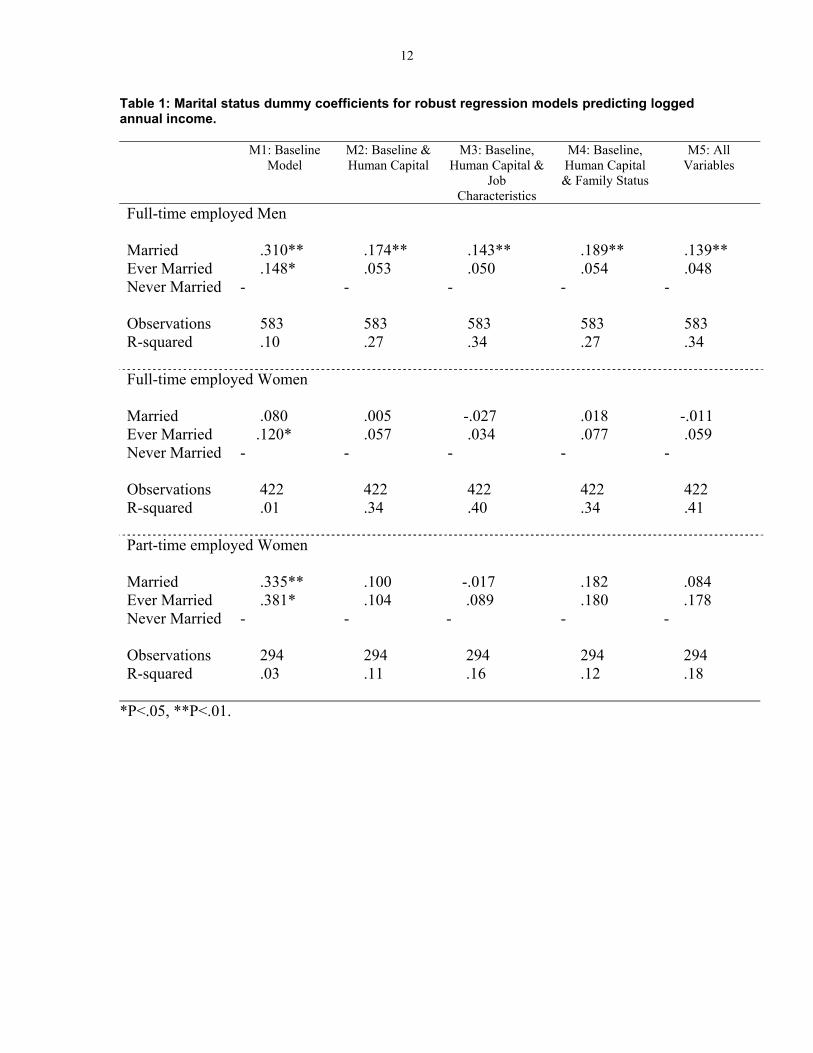
Our examination of the relationship between earnings and marriage shows a large

and significant marriage premium for men, but little or no association between marriage

and income for women. Adjusting for a range of human capital, job, and family

characteristics and confining the sample to those who were employed at the time of the

survey (excluding the self employed), married men in our study earn 15 per cent more, on

average, than unmarried men. We found little or no association between marriage and

women’s income.

Our conclusion then is that marriage is good for men in terms of earnings. While

marriage has no impact on women’s earnings, it may be that, marriage improves

women’s overall standard of living, insofar as they have access to their husband’s

earnings.

1 This section of the paper is adapted from an earlier paper by Belinda Hewitt, Mark Western and Janeen

Baxter (2002) titled “Marriage and Money: The Impact of Marriage on Men’s and Women’s Earnings.”

12

Table 1: Marital status dummy coefficients for robust regression models predicting logged annual income. M1: Baseline

Model M2: Baseline & Human Capital

M3: Baseline, Human Capital &

Job Characteristics

M4: Baseline, Human Capital & Family Status

M5: All Variables

Full-time employed Men Married .310** .174** .143** .189** .139** Ever Married .148* .053 .050 .054 .048 Never Married - - - - - Observations 583 583 583 583 583 R-squared .10 .27 .34 .27 .34 Full-time employed Women Married .080 .005 -.027 .018 -.011 Ever Married .120* .057 .034 .077 .059 Never Married - - - - - Observations 422 422 422 422 422 R-squared .01 .34 .40 .34 .41 Part-time employed Women Married .335** .100 -.017 .182 .084 Ever Married .381* .104 .089 .180 .178 Never Married - - - - - Observations 294 294 294 294 294 R-squared .03 .11 .16 .12 .18

*P<.05, **P<.01.

13

The Housework Burden

Research has consistently shown that wives do more domestic labour than their husbands

(Berk, 1985; Shelton, 1992; Baxter, 1993; Brines, 1994; Bittman, 1995, 1998; Bianchi

et.al., 2000). Feminist reformers in the 1960s and 1970s were optimistic that changes in

the labour force participation rates for married women, in combination with increased

awareness of the value of women’s unpaid work in the home, would lead to an increased

involvement of men in domestic labour and a more equal domestic division of labour

between men and women (Gavron, 1983; Oakley, 1974). To a large extent, this has not

happened. It is largely indisputed that women do approximately three quarters of

household work, a pattern that is evident across all western nations (Szalai, 1972; Berk,

1985; Baxter, 1997).

Our current data show that women do a significantly larger proportion of

childcare and routine housework tasks than men regardless of marital status and spend

considerably more time on housework than men (19 to 25 hours per week compared to

eight hours per week for men). Unfortunately we are not able to compare the differences

between single and married women with these data, as single people were not asked the

questions on domestic labour. However, we can compare the patterns of couples living in

defacto relationships with those living in married relationships. In some ways this

comparison focuses the analyses more sharply on the impact of marriage, as living

arrangements are held constant across both groups and the only difference is legal marital

status.

The results show that men in de facto relationships do a greater proportion of

indoor housework tasks than married men (40% compared to 26%) and a smaller

proportion of outdoor tasks (73% compared to 83%). But there is no difference in the

amount of time that men in these groups spend on housework with both spending

approximately nine hours per week. For women however there is a significant difference

in time spent on housework according to marital status with married women spending

approximately 6 additional hours per week compared to women in de facto relationships.

Women in de facto relationships also do a much smaller proportion of indoor tasks.

14

These patterns remain when we control for possible socio-demographic

differences between de facto and married couples that might explain these differences

including age of the couple, presence of children, gender role attitudes, education, labour

market status and earnings.

In terms of domestic labour then, the results are very clear-cut. Marriage clearly

benefits men and has negative consequences for women.

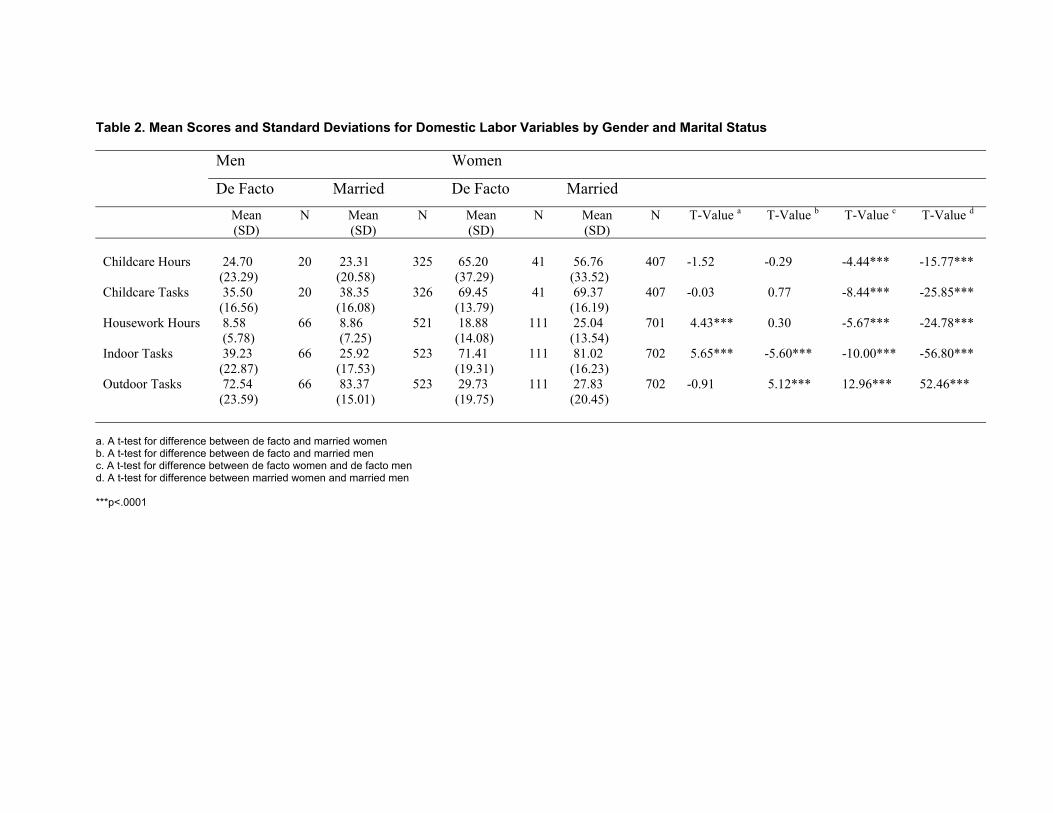
Table 2. Mean Scores and Standard Deviations for Domestic Labor Variables by Gender and Marital Status

Men Women De Facto Married De Facto Married

Mean(SD)

N Mean(SD)

N Mean(SD)

N Mean(SD)

N T-Value a T-Value b T-Value c T-Value d

Childcare Hours 24.70

(23.29) 20 23.31

(20.58) 325 65.20

(37.29) 41 56.76

(33.52) 407 -1.52 -0.29 -4.44*** -15.77***

Childcare Tasks 35.50 (16.56)

20 38.35 (16.08)

326 69.45 (13.79)

41 69.37 (16.19)

407 -0.03 0.77 -8.44*** -25.85***

Housework Hours 8.58 (5.78)

66 8.86 (7.25)

521 18.88 (14.08)

111 25.04 (13.54)

701 4.43*** 0.30 -5.67*** -24.78***

Indoor Tasks 39.23 (22.87)

66 25.92 (17.53)

523 71.41 (19.31)

111 81.02 (16.23)

702 5.65*** -5.60*** -10.00*** -56.80***

Outdoor Tasks 72.54 (23.59)

66 83.37 (15.01)

523 29.73 (19.75)

111 27.83 (20.45)

702 -0.91 5.12*** 12.96*** 52.46***

a. A t-test for difference between de facto and married women b. A t-test for difference between de facto and married men c. A t-test for difference between de facto women and de facto men d. A t-test for difference between married women and married men ***p<.0001

Conclusion

The two areas of research that have been covered in this paper, labour force and

household labour, demonstrate the direction of research of the current project. The

work/family sphere is pertinent to sociological analyses of the family, and this research

advances debate on the institution of marriage and its association with the experiences of

men and women.

The findings show that both gender and marriage are associated with paid and

household labour. Although research has consistently shown the division of labour by

gender, the marriage effect has not been as well documented. This research finds that

married men fare better in the workplace than both cohabiting and single men, and that

marriage has clear benefits in terms of domestic labour.

The future focus of this research is to examine the relationship between marriage

and other aspects of life, such as work satisfaction, self-perception, wellbeing and

attitudes. This will contribute to the debate on the benefits, or otherwise, of marriage.

17

Bibliography Bachrach, C., Hindin, M. and Thomson, E. (2000). The changing shape of ties that bind: An overview and synthesis. In L. Waite (ed.) The ties that bind: Perspectives on marriage and cohabitation. New York: Walter de Gruyter Inc. pp: 3–18.

Baxter, J. (1993) Work at Home. St Lucia: UQP.

Baxter, J. (1997) Gender Equality and Participation in Housework: A cross national perspective. Journal of Comparative Family Studies 28(3): 220–47.

Beck, U. and Beck-Gernsheim, E. (1995) The Normal Chaos of Love. Cambridge, UK: Polity Press.

Becker, G. 1985. Human Capital Effort, and the Sexual Division of Labor. Journal of Labor Economics 3: S33–S58.

Beck-Gernsheim, E. (2002) Reinventing the family: in search of new lifestyles. Cambridge, UK ; Malden, MA : Polity.

Berk, S. (1985) The gender factory: the apportionment of work in American households. New York: Plenum Press.

Bernard, J. (1982) The Future of Marriage. New Haven: Yale University Press.

Bianchi, S., Milkie, M., Sayer, L. and Robinson, J. (2000). Is Anyone Doing the Housework? Trends in the Gender Division of Household Labor. Social Forces 79(1): 191–228.

Bittman, M. (1995) The Politics of the Study of Unpaid Work. Just Policy. 2: 3–10.

Bittman, M. (1998) Land of the lost long weekend-trends of free time among working age Australians 1974–1992. SPRC Discussion Paper No. 83. Kensington: Social Policy Research Centre, University of New South Wales.

Blackburn, McKinley and Korenman, S. (1994). The declining marital-status earnings differential. Journal of Population Economics. 7:247–270.

Brines, J. (1994). Economic Dependency, Gender and the Division of Labor at Home. American Journal of Sociology. 100(3): 652–688.

Chalmers, J. (2002). Why Marry? An economic analysis of the male marriage premium. Unpublished PhD Thesis: Australian National University.

Chapman, B., Dunlop, Y., Gray, M., Liu, A. and Mitchell, D. (2001). The impact of children on the lifetime earnings of Australian women: Evidence from the 1990s. The Australian Economic Review. 34(4): 1–17.

Davies, H., Joshi, H. and Peronaci, R. (2000). Forgone income and motherhood: What do recent British data tell us? Population Studies. 54: 293–305.

De Vaus, D. (2002) Marriage and Mental Health. Family Matters. 62: 26–32.

De Vaus, D. and Wolcott, I. (eds.). (1997). Australian Family Profiles: social and demographic patterns. Melbourne: Australian Institute of Family Studies.

Desai, S. and Waite, L. (1991). Women’s employment during pregnancy and after the first birth: Occupational characteristics and work commitment. American Sociological Review. 56(4): 551–66.

Dolton, P. and Makepeace, G. (1987). Marital Status, Child Rearing and Earnings Differentials in the Graduate labor Market. The Economic Journal. 97: 987–922.

Gavron, H. (1983). The captive wife: conflicts of housebound mothers. London : Routledge & Kegan Paul.

Giddens, A. (2001). The global revolution in family and personal life, in A. Skolnick and J.Skolnick (eds), The family in transition. Boston, Allyn and Bacon.

Ginther, D. and Zavodny, M. (2001). Is the male marriage premium due to selection? The effect of shotgun weddings on the return to marriage. Journal of Population Economics. 14: 313–328.

18

Gornick, J. (1999). Gender equality in the labour market. in D. Sainsbury (ed.) Gender and welfare state regimes. Oxford University Press: Oxford. pp: 210–42.

Gray, E. and McDonald, P. (2002). The relationship between personal, family, resource and work factors and maternal employment in Australia. Organisation for Economic Co-operation and Development, Labour Market and Social Policy Occasional Papers No. 62.Paris: OECD.

Gray, J. (1997). The Fall in Men’s Return to Marriage. The Journal of Human Resources. 32: 481–504.

Hill, M. (1979). The Wage Effects of Marital Status and Children. The Journal of Human Resources. 14: 579–594.

Korenman, S. and Neumark, D. (1991). Does marriage really make men more productive? Journal of Human Resources. 26: 282–307.

Korenman, S. and Neumark, D. (1992). Marriage, motherhood and wages. Journal of Human Resources. 27: 233–55.

Loh, E. (1996). Productivity Differences and the Marriage Wage Premium for White Males. The Journal of Human Resources. 31: 566–589.

McDonald, P, Jones, F., Mitchell, D. and Baxter, J. (2000). Negotiating the Life Course, 1997 [computer file]. Canberra: Social Science Data Archives (SSDA), The Australian National University.

McLaughlin, S. (1982). Differential patterns of female labor-force participation surrounding the first birth. Journal of Marriage and the Family. 44: 407–20.

Oakley, A. (1974) The Sociology of Housework New York: Pantheon Books.

Richardson, K. (2000). The evolution of the labor premium in the Swedish labor market 1968–1991. Scandinavian Working Papers in Economics No. 2000-5. Institute for Labour Market Policy Evaluation.

Shelton, B. (1992). Women, Men and Time: Gender Differences in Paid Work, Housework and Leisure. Westport, CT: Greenwood.

Szalai, A (ed). (1972) The use of time: Daily activities of urban and suburban populations in twelve countries. The Hague : Mouton

Waite, L and Gallagher, M. (2000) The case for marriage: why married people are happier, healthier, and better off financially. Broadway Books: New York.

Waldfogel, J. (1997). The effect of children on women’s wages. American Sociological Review. 62: 209–17.

19

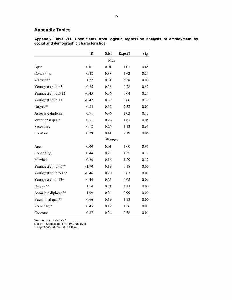
Appendix Tables Appendix Table W1: Coefficients from logistic regression analysis of employment by social and demographic characteristics. B S.E. Exp(B) Sig.

Men

Ager 0.01 0.01 1.01 0.48

Cohabiting 0.48 0.38 1.62 0.21

Married** 1.27 0.31 3.58 0.00

Youngest child <5 -0.25 0.38 0.78 0.52

Youngest child 5-12 -0.45 0.36 0.64 0.21

Youngest child 13+ -0.42 0.39 0.66 0.29

Degree** 0.84 0.32 2.32 0.01

Associate diploma 0.71 0.46 2.03 0.13

Vocational qual* 0.51 0.26 1.67 0.05

Secondary 0.12 0.26 1.13 0.65

Constant 0.79 0.41 2.19 0.06

Women

Ager 0.00 0.01 1.00 0.95

Cohabiting 0.44 0.27 1.55 0.11

Married 0.26 0.16 1.29 0.12

Youngest child <5** -1.70 0.19 0.18 0.00

Youngest child 5-12* -0.46 0.20 0.63 0.02

Youngest child 13+ -0.44 0.23 0.65 0.06

Degree** 1.14 0.21 3.13 0.00

Associate diploma** 1.09 0.24 2.99 0.00

Vocational qual** 0.66 0.19 1.93 0.00

Secondary* 0.45 0.19 1.56 0.02

Constant 0.87 0.34 2.38 0.01

Source: NLC data 1997. Notes: * Significant at the P<0.05 level. ** Significant at the P<0.01 level.

20

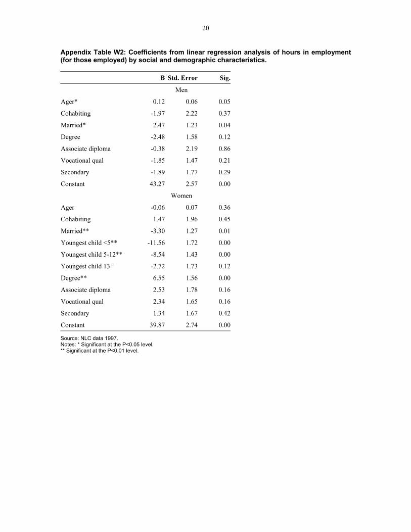
Appendix Table W2: Coefficients from linear regression analysis of hours in employment (for those employed) by social and demographic characteristics. B Std. Error Sig.

Men

Ager* 0.12 0.06 0.05

Cohabiting -1.97 2.22 0.37

Married* 2.47 1.23 0.04

Degree -2.48 1.58 0.12

Associate diploma -0.38 2.19 0.86

Vocational qual -1.85 1.47 0.21

Secondary -1.89 1.77 0.29

Constant 43.27 2.57 0.00

Women

Ager -0.06 0.07 0.36

Cohabiting 1.47 1.96 0.45

Married** -3.30 1.27 0.01

Youngest child <5** -11.56 1.72 0.00

Youngest child 5-12** -8.54 1.43 0.00

Youngest child 13+ -2.72 1.73 0.12

Degree** 6.55 1.56 0.00

Associate diploma 2.53 1.78 0.16

Vocational qual 2.34 1.65 0.16

Secondary 1.34 1.67 0.42

Constant 39.87 2.74 0.00

Source: NLC data 1997. Notes: * Significant at the P<0.05 level. ** Significant at the P<0.01 level.

21

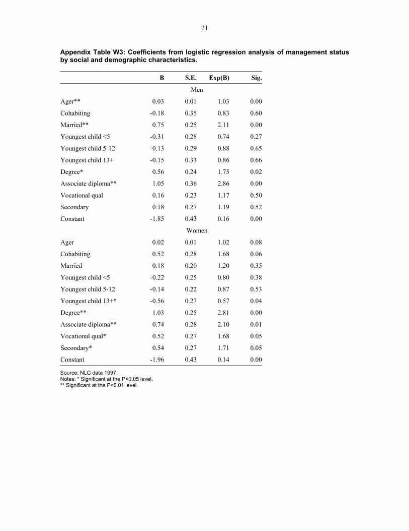
Appendix Table W3: Coefficients from logistic regression analysis of management status by social and demographic characteristics. B S.E. Exp(B) Sig.

Men

Ager** 0.03 0.01 1.03 0.00

Cohabiting -0.18 0.35 0.83 0.60

Married** 0.75 0.25 2.11 0.00

Youngest child <5 -0.31 0.28 0.74 0.27

Youngest child 5-12 -0.13 0.29 0.88 0.65

Youngest child 13+ -0.15 0.33 0.86 0.66

Degree* 0.56 0.24 1.75 0.02

Associate diploma** 1.05 0.36 2.86 0.00

Vocational qual 0.16 0.23 1.17 0.50

Secondary 0.18 0.27 1.19 0.52

Constant -1.85 0.43 0.16 0.00

Women

Ager 0.02 0.01 1.02 0.08

Cohabiting 0.52 0.28 1.68 0.06

Married 0.18 0.20 1.20 0.35

Youngest child <5 -0.22 0.25 0.80 0.38

Youngest child 5-12 -0.14 0.22 0.87 0.53

Youngest child 13+* -0.56 0.27 0.57 0.04

Degree** 1.03 0.25 2.81 0.00

Associate diploma** 0.74 0.28 2.10 0.01

Vocational qual* 0.52 0.27 1.68 0.05

Secondary* 0.54 0.27 1.71 0.05

Constant -1.96 0.43 0.14 0.00

Source: NLC data 1997. Notes: * Significant at the P<0.05 level. ** Significant at the P<0.01 level.