:I.e r,tl94 Al4t~JI

Co $IVIL ENGINEERING STUDIES l' Y ",-, STRUCTURAL RESEARCH SERIES NO. 238

.~

-AN ACCELERATED mRATIVE PROCEDURE

FOR SOLVING PARTIALLQ1!FERENCE EQUATIONS

OF ~IPTIC TYPE

By . ."....-.

JS~ J?~~i. DOSHI

and

A Report on a Research

Program Carried out

under

National Science Foundation

Grant No. G-6572

UNIVERSITY OF ILLINOIS

URBANA, ILLINOIS

APRIL, 1962

6

55

FIG 0 5

ERRATA

AN ACCELERATED ITERATIVE PROCEDURE FOR SOLVING

PARTIAL DIFFERENCE EQUATIONS OF ELLIPTIC TI"PE

University of Illinois Civil Engineering Studies

Structural Research Series No u 238

by K. D. Dc,shi and A. Alles

ERRORS

Insert "A" in last line of Eq. (2.,3).~ to read~

H(v) + J(V) A = I.

Insert II the" in line 7, 2nd paragraph) to read.: ...... in the absence of ...... .

Add "to such a procedure.!! to the last sentence on this page 0

Change rlpOSITIVE" to "NEGATIVErl in the title.

10

AN ACCELERATED ITERATIVE PROCEDURE fOR SOLVING PARTIAL

DIFFERENCE EQUATIONS OF ELLIPTIC TYPE

Kishor Dharamsi Doshi) PhoDo

Department of Civil Engineering

University of Illinois; 1962

This thesis deals with certain iterative methods of solving finite

difference equations arising from elliptic type boundary-value problemso

A procedure that accelerates the convergence of explicit) linear iterative

methods of first degree is presented 0 The concept of acceleration implied

here is similar to the one expressed in Hotelling~s matrix squaring procedure

in which the iterative sequence is advanced by a nuraber of cycles at a time 0

Certain simplifying assumptions are made in the formulation of

the acceleration scheme and as a result) some of the error components are

diminished in the process) while others are magnifiedv A detailed study

of the error and convergence associated with the acceleration scheme is

presented.

To substantiate the conclusions from analytical study) the

procedure is studied in connection with the problem of plates on elastic

foundation using the proposed scheme in conjunction with the successive

over-relaxation method 0

The results clearly indicate the effectiveness of the prOCedure

presentedo

11

ACKNOWLEDGElvlliNT

This thesis was written under the immediate direction of Dr. A. Ang)

Assistant Professor of Civil Engi~eering, and the study was made possible by

a grant from the National Science Foundation.

The author wishes to express his sincere appreciation to Dr. A. Ang

for having introduced him to the general subject of iteration and for his

suggestions in the course of the investigation. The author also wishes to

acknowledge the encouragement of his academic adviser} Dr. Co P. Siess)

Professor of Civil Engineering.

Thames are also due to the 'ILLIAC' personnel for their cooperation)

and to Miss Virginia Carr for the painstw{ing care she took in typing the

iterating equations.

12

iii

TABLE OF CONTENTS

1. IN'rRODUCTION .••. 0 ••••••••••••••• 0 ••••••• 0 " 0 • 0 • 0 ••• 0 •••••••••• 0 0 • < 0 • 0 1

1 . 1 Ob j e ct. . 0 0 • 0 • • 0 • 0 0 0 0 , • • • " 0 0 • • • 0 • • 0 0 0 0 • • • • • • 0 • • • • • 0 0 • " 0 • .. • 1 1.2 statement of the Problem. 0 0 • 0 " •• 0 0 ., 0 •••• 0 ••••• 0 • n 0 0 •••• 0 • 2 1.3 Iterative Methods in General ......•••........•.••.•. " .... 4

2. EXPLICIT IT:E:RATIVE J'.1ETHODS .• 0 ••••••••••• 0 n •••• 0 , •• no •••••••• 0 • 0 0 0 • • • • 5

2.1 Introductory Remarl(s .•••••..... · ......•.............• o.n •• 5 2.2 General Linear Iterative Processes of First Degree ...•... 5 2.3 Certain Stationary Iterative Procedures ..... , ......•. n ••• 8 204 Convergence Criteria .... 0 •••• 0 " 0 •• 0 0 0 •• 0 •••••• , •• ? 0 • " • 0 " •• 13

3. TIrE J1J1v1P SCI£E:t-£E. 0 •• 0 0 0 •• 0 • 0 ••••••• " •• , •••••••• 0 • 0 •• 0 •••• 0 • 0 • • • • • • • •• 16

3.1 Introductory Remarks ..•.•••......••...•.. 0 • n , 0 •••••• 0 n •• ,. 16 3 . 2 General Background ...•. 0 " • no ••••••• 0 •••• , •• n •• 0 •• n • 0 •• 0 •• 16 3.3 The Scheme. 0 0 • 0 •• no ••••••• 0 •••• 0 •••••••• 0 0 • " ••• 0 • " •• " ••• " 20

4. EVALUATION

4.1 4.2 4·3

OF T:HE JU1.1:P SCJm1E. 0 0 0 •• 0 0 0 0 • 0 • 0 n 0 0 • 0 • " • 0 " 0 n •• 0 • 0 • n " 0 ••• 0 26

Introductory Remarks .. 0 •• 0 0 0 0 ., •• " 0 0 • 0 • 0 • 0 , n •• 0 •• 0 0 , 0 • " n 0 0 26 General Background. 0 •• 0 0 0 0 0 • 0 u 0 , 0 •• 0 0 • 0 0 0 coo 0 ••• , 0 0 , 0 0 ., C • 0 26 Loss 8.I1d Gain .Arlalysis 0 < ? 0 ~ • 0 • " coo. 0 0 0 " 0 0 0 • 0 0 •• 0 0 0 0 0 • 0 0 0 ,. 33

4 0 3 • 1 w s s Analys is ..•.• 0 0 0 • 0 ••• 0 0 0 0 0 0 0 • 0 ~ • 0 • 0 0 0 • a', 35 40302 Gain Allalys is 0 • 0 0 0 ,. 0 0 0 0 0 • 0 • 0 •• 0 • 0 0 0 • 0 " 0 • 0 • 0 •• 40

4.4 Numerical Study of Variables 0 • ,. a ~ 0 0 0 0 0 U • 0 •• 0 , ••• 0 0 • <, ••• 0 • 0 43

4 0 4 . 1 I..o s s Analy sis • c. 0 .) 0 0 0 0 0 0 0 " • e e , 0 0 eo!' 0 ? 0 0 • " ., 0 • 0 0 45 40 40 2 Gain Allalys is. 0 0 n 0 0 0 0 0 0 " 0 • 0 • 0 0 • 0 •• 0 • 0 • 0 0 0 0 0 0 0 46

4.5 Modified Jump Scheme 0 ••• , • 0 0 •• 0 •• 0 0 • 0 • " " •• 0 0 u " • 0 0 0 •• 0 " •• 0" 48

5 . EXPERIMENTS VlITH THE JUMP SCHEME 0 0 n " ••• 0 •• 0 U 0 Q !' 0 0 0 0 0 , 0 0 0 0 0 0 0 ~ 0 • 0 ••• ? 49

5 0 1 Introductory Remarks ..• 0 0 0 0 , •••• 0 0 0 0 • 0 0 •••• 0 0 ••• 0 • 0 0 ••• 0 •• 49 5.2 The l1ethod of Successive Over-Relaxation.o." •• , ... " .• oOO" 49 5 " :5 A Special Result. coo 0 0 0 0 •••• 0 0 0 Q • 0 • 0 0 0 • 0 • 0 !' • 0 0 0 0 ., 0 " U " 0 0 0 0 51 504 Discussion of Results. " 0 0 U 0 00. 0 0 0 0 0 " 0 •• , 0 0 0 0 U • 0 0 0 • no" 0 0 0 0" 52

6 . SUMNARY AND CONCLUSIONS ••.•. 0 •• 0 • 0 0 0 0 0 0 • 0 0 0 •• Q 0 • 0 ••• 0 0 0 no. 0 0 • U • 0 • 0 • n 54

6.1 Su.rrnnary of the Study 0 • 0 0 • Q 0 • 0 0 . 0 • " • n u • 0 • 0 " 0 0 • 0 • 0 • 0 0 co. 0 0 0 54 602 Conclus ions .. 0 . 0 0 ••• n .. 0 0 • 0 •. , •• 0 0 U " •• 0 • " 0 0 • 0 • 0 0 • 0 0 • , 0 " 0 • 0 n 55

BIBLIOGRA.PlIT 0 • 0 0 u 0 0 0 • 0 0 " •• 0 • 0 0 0 0 0 •• 0 • u 0 0 0 0 0 0 • 0 a •• 0 a 0 0 0 •• 0 • 0 •• 0 0 " ., 0 •• 0 0 0 n 56 TABLES 0 • • 0 0 0 • 0 0 0 0 0 0 • 0 0 • 0 • • 0 0 • • 0 • 0 0 0 0 0 ., 0 0 0 0 • 0 0 0 0 0 " 0 0 0 0 • • U , 0 0 0 0 0 • 0 ., 0 0 • 0 • o. 57 FIGURES 0 Coo 0 0 0 0' 0 0 0 0 0 0 I) I) a I) 0 0 0 0 0' 0 I) 0 0 0 0 0 0 I) 'III 0 0 " 0.0 0 0 0 0 0 0 0' 0 0 0 coo I) " 0 I) ,., I) 0 I) 0 I) " 0 I) 0 67 VITA 0 (I I) 0 0 • 0 0 0 I) 0' 0 0 0 ~ (I 0 0 (I 0 0 0 0 0 0 0 I) 0 a 0 I'J 0 0 0 0 0 0 I.' 0 0 (I 0 0 0 0 0 (I II I) 0 0 0 0 IJ 0 0 0 (I 0 'III 0 0 ~~ 0 " ('I \) I.l 72

13

1.1 Object

CHA.PrER 1

INTRODUCTION

Boundary value problems in engineering and science often lead to

partial differential equations of the elliptic type. The solution of these

equations constitutes a major problem for those interested in obtaining

numerical results. Since analytical or closed form solutions can be found

for only a few cases, approximate methods play an important role. Of these)

the method of finite differences is one of the most wid~ly used techniques)

and has been increasingly used since the development of modern digital

computing machines.

Basically, the finite difference method involves discretization

of a continuum, thus leading to a solution in the form of a function defined

at discrete points rather than at every point in a region. In this process,

differentials are replaced by finite increments, and derivatives by finite

difference quotients} and a partial differential equation is then replaced

by a system of finite difference equations. Each finite difference equation

defines the state of one point) as an implicit function of the variables

defined at points in the neighborhood. When this is done for each of the

discrete points in the continuum, a partial differential equation reduces to

a set of simultaneous, algebraic equations.

In this study, only finite difference approximations to linear

partial differential equations of elliptic type are considered. Theoretically,

solving the resulting system of simultaneous, linear, algebraiC equations

presents no problem. However, the task of obtaining a numerical solution by

by i terati ve'~ltechniques presents interesting problems of convergence.

1

14

Quite often large systems of e~uations are encountered and one is

then confronted with a problem of developing techniques to minimize the amount

of computational work. Since iterative methods are well-suited for solving

partial difference equations of elliptic type) they are widely used for such

a purpose. In this case one is primarily concerned with improving the rate

of convergence of solution. In this study) the system of e~uations are

assumed to have no ill-condition property.

A procedure called "Jump Scheme tl is presented in Chapter 3) and is

developed for use in conjunction with certain iterative methods of solving

linear) partial differential equations of elliptic type.

1.2 statement of the Problem

As indicated previously) the approximation of a linear partial

differential equation by finite differences leads to a set of linear;

simultaneous equations. These equations can be written in general as:

where

n ~

j=l a .. x. lJ J

d. l

x~ :s the dependent variable)

(i

a " is a coefficient from finite difference ~uotient) and ~L

c is a constant.

USi~b ~atrix notation) this can be written in the form~

Ax d

where A [a .. ] lJ n x n)

x [x. ] l' and J n x

[diJn x ~ 15

d

2

.3

Note that if A is non-singular) the matrix Equation (1.2) is satisfied on.ly for

* * -1 x x where x is the exact solution and x = A d.

The task is thus reduced to obtaining a solution of Equation (1.1)

or (1.2) consistent with the boundary restraints specified in the physical

problem. By a solution is implied the determination of a vector x such that

* it deviates from the exact solution x by a specified tolerance. Stated

differently) this means that)

II x - x* II < 5

where 5 is a preassigned scalar constant.

Hence) the problem is to develop a method of determining the solution

vector x consistent with boundary restraints. This method should) however)

fully utilize the properties of the matrix Ao Some of these properties are~

1. The matrix A is of large order n ranging from perhaps forty to

some thousands.

2. A is a "sparse" matrix since the proportion of non-zero elements

is very small. For plate problem (involving bibarmonic elu,a.tion) for example)

the central-difference operator yields at the most thirteen non-zero elements

in any row of A.

3. In many cases) the nOD-zero elements of A are easy to generate

from the problem whenever they are needed and hence m~y not have to occupy

the valuable storage space in the computer. Thus A can be a Ilgenerated matrix"

instead of a "stored matrix. II

4. In many cases) the matrix A is symmetric.

5. Most linear boundary value problems which amount to minimizing

an energy can be discretized as matrix problems with a definite) symmetric

matrix Ao Definiteness of A greatly aids the solution by almost any method.

16

4

103 Iterative Methods in General

~1ethods for solving the system of e~uation (1.2) can be broadly

classified into "direct" and "iterative" methods. Direct methods) of which

the solution by elimination is typical) would yield the exact answer in a

finite number of steps if there were no round-off error. Usually) the algorithm

of a direct method is rather complicated and nonrepetitiouso Iterative methods)

on the other hand) involve repeated application of a simple algorithm) and

ordinarily yield the exact answer only as a limit of a se~uence even if no

round-off error is present.

Iterative methods are preferred for solving large) sparse systems

(102) because they can usually take full advantage of the numerous zeros in

A) both in storage and in operation. They can) in general) be divided into

two principal groups as Ifexplicitfl and flimplicit ll iterative methods. In explicit

iterative methods) the v th approximation to the i th component of the solution

vector x is determined by itself at its proper step in iteration) without the

necessity of simultaneously determining a group Qf other components of x.

In contrast are the implicit iterative methods in which) a group of components

of the vector x are defined simultaneously in such an interrelated manner that

it is necessary to solve a linear subsystem for the whole subset of components

at once before a single one can be determined. ~JPical of these methods are

4-¥-the Peaceman-Rachford (1955) and Douglas-Rachford (1956) methods '.

Only explicit iterative methods are discussed in the remainder of

this thesis.

* These numbers refer to corresponding entries in the Bibliography.

17

CHAPTER 2

EXPLICIT ITERATIVE }'1ETHODS

201 Introductory Remarks

As indicated earlier) iterative methods for the solution of a set

of simultaneous equations are characterized by a successive improvement of

an arbitrarily assumed solution vector x(O)o The improvement is achieved

through a repeated application of a simple algorithm) and the process yields

the exact answer only as the limit of a sequence. Improvement is possible

only) of course) if the process is a converging one. Cr~teria of con-

vergence will be discussed later in-this chapter 0 In all subsequent

discussion) however) convergence of the process is implied.

For linear iterative methods) starting with an arbitrarily assumed

(v+l) x )

in such a \-lay that x(V+l) is a linear function of x(V), x(V-l)) .,.oo"x(l))

( n '\ ( l' , ( v !-1 ) x' '-/ /) where x\· / is the vth solution vectoro If x" -. -, does not depend on

(v-l) (v-2) (0) 3 x ) x ) 0000 oX ) then the method is said to be of IIfirst degree" .)

Among linear iterative processes of first degree are the methods of

simultaneous displacement, successive displacement) and successive over-

relaxation. An example of an iterative process of second degree is the

extrapolated Richardsonvs procedure50

Only linear iterative processes of first degree will be discussed

in the remainder of this thesis.

2.2 General Linear Iterative Processes of First DeGree

For the system of Eqso (1.2)

Ax

5 18

d (1.2)

the most general linear iterative method of first degree having the property

that: (1) it is independent of the vector d) and (2) X(k) = x* impiies

x(p) = x* (p ~ k)) can be stated as follows 6

Denote by c(v) (v = 0)1)2 .... )) a nonsingular s~uare matrix of

order n) which for all v is different from _A-I. In general) C(v) is a

function of v. Starting from an arbitrarily assumed v"ector :;/0)) a new

t ( v+l) . . 1 d . d f (v) ( 0 1 2 ) b vec or x lS succeSSlve y erlve rom x v = ) ) •...• y means

of this iteration matrix C(v) as follows:

or

(v+l) x

x (v+l)

where I is an identity matrix of order n.

(2.2)

A completely e~uivalent set) and sometimes a more convenient fonn

to use) is 3:

x (v+l)

where

and)

The vth !lerror vector" z(v) is defined as:

z (v) (v) * x - x (2.,4)

z (v+l) (v+l) * x - x (2 0 4a)

19

6

Hence)

From (2.1))

Therefore)

and

from which)

(v+l) (v) (v+l) (v) z - z = x - x

X(v+l) _ xCv) = C(v) [Ax(v) _ d]

= c ( v) [Ax ( v) - Ax * ]

(v+l) z = [I + c(v) A] z

(v)

z (v)

* (since Ax = d)

(2,,6)

Thus) the error vector z(v+l) satisfies the fundamental iterations

(2.2) and (2.3) with d set equal to zero.

In the general forms (2.1) and (203)) the iteration matrices C(v)

and R(v) are dependent on v. Such iterative processes are termed

"nonstationary." If the matrix C or H is independent of v) the iterative

7

process is said to be "stationary.1I For stationary processes) reations (201))

(2.2)) (2.3)) (2.5)) wld (2.6) redUCe respectively to:

x (v+l) = x( v) + C [Ax( v) - d] (207)

x (v+l) [I + CA] x ( v) - Cd (2.8)

x (v+l) = Hx(v+l) + Jd (2.9)

20

8

where H I + CA,

J C,

and R + JA I

z (v+l) = (I + CA) z

(v)

and Z (v+l)

= HZ(v)

The aim of every iterative process is to make the error vector

(v+l) z converge to null vector as fast as possible. Using (2.11) v times)

one gets:

(2.12)

The matrix H thus operates upon the error vector z(O) in every cycle)

forcing it to converge to the null vector ultimately. Because of the role it

plays) the matrix H constitutes a focal point in the study of convergence of

linear iterative procedureso

2.3 Certain Stationary Iterative Procedures

A discussion of some of the better known stationary iterative

procedures is given in the following sections. These are the simultaneous

displacements) successive displacements and successive over-relaxation methodso

For a matrix representation of the different procedures) the matrix

A is partitioned into:

A=L+D+V

where: L is the lower triangular matrix of A (i > j) with the diagonal

elements equal to zeroj

D is the diagonal matrix of A (i j);

21

9

and) U is the upper triangular matrix of A (i < j) with the diagonal

elements equal to zero.

One then proceeds to solve the system (1.2) as:

(L + D + U)x = d (1.2a)

(a) Method of Simultaneous Displacements

The method of simultaneous displacements was first proposed by

Jacobi in 18458. Starting with an arbitrarily assumed vector x(O)) the

vector x(V-l)) after (v-I) iterations is obtained. One then evaluates the

rth component) x (v)) of the succe~ding iteration by solving the rth equation r

of Ax = d forJx (v) or) r )

(v-I) I x 1 +0 •••• + a

r+ r+ rn x

n (v-I)

d r

(r .. ;;; 1)2)" 0.0. on)

In (2.14)) a one-to-one correspondence between the n unknowns x r

and the n equations in Ax = d is assumed to exist) so that each equation is

solved fer t~e corresponding unknown. Such a correspondence is naturally

satisf~ed in :inite difference approximations to a partial differential

equatior ..

Ii:)te that the n equations are independent and hence may be solved

in an:,' o:-de:-.

In rratrix notation) one finds x(v) by solving:

Lx(V-l) + DX(v) + Ux(v-l) = d (2.15)

or (2016)

Comparing (2.16) and (2.3)) the iteration matrix H in the method of

22

10

simultaneous displacements can be expressed as~

H (2017)

J - D -1

(2017a)

In a similar procedure called the method of steepest descent, one

finds x(v) from:

x (v)

where a is a scalar constant.

In this case, H = I - aA - (2019)

The constant a is selected to give the fastest convergence. The

method, however, is developed for symmetric) positive definite matrices only.,

(b) Method of Successive Displacements

This method is also known as the Gauss-Seidel method1. It may

be considered as a variant of the method of simultaneous displacements. The

variation consists in using a new component x (v) in E~so (2.14) as soon as r

it has been computed 0

In addition to the one-to-one correspondence between the n unknowns

x. and the n e~uations as assumed in the method of simultaneous displacements, l

one has now to fix a certain cyclic order 0 (l,2 ... oon) in which the components

x. will be computed. With these requirements, the method of successive l

displacements is defined by changing (2.14) so that it reads:

(v-l) + a 1 x 1 +0 •... + a r) r+ r+ rn

23

x n (v-l)

d r

+ a rr

(r

X r

(1/)

(2.20) 1,2,.00 oen)

Thus) when solving (2020) for the conponent x (v) one a.lways uses r

the latest values of all other components ~ Thi.s means that only a single

vector x has to be stored in the computer at a time) as compared to the

method of simultaneous displacements where one has to store a portion of

both x(v-l) and x(v).

In matrix notation) the present method solves the equation:

U (v-I) + x d

or

Comparing (2.22) and (203)) the iteration matrix H for the method of

successive displacements can be written as~

H

Also) J

(c) Successive Over-Relaxation Method (S.O.R.)

The method of successive over-relaxation developed independently

1- ~

by YOunb .L and Frankel) is essentially a modification of the successive

displacements method 0 The modification) hOI-lever) greatly accelerates corJ-

ver8ence in certain types of problemso

In this (v) method) one computes the components x. . of the vector

l

(v) x' from the set of values x. (v-l) (i = 1,2" 0 0. on); in two staGes~

l

First an inteTIllediate value x (v) is obtained in a sim:i.lar I'

fashion as is done in the method of successive displacementso Thus) one

solves~

a x (v) + a x (v) rl 1 r2 2

a x (v) r)r-l r-l + a rr

x r (v)

:1:1

(v-l) + a x r)r+l. r+l +00000+ a rn x

n (v-l)

d I'

(r

(2.24)

1,2,oo<,00n)

24

In the second stage) the value of x (v) is computed from: r

I

12

x r (v) x (v-l) + w[x (v)

r r _ x (V-I)]

r (2.25)

where 1 < w < 2 is the over-relaxation factor.

Durin8 computation) only a single vector x has to be stored at

(v) (v-I) anyone time since the new value x replaces x as soon as the new r r

value is computed. I

In matrix notation) to obtain the vector xCv) ) one solves the

equation: - I

Lx(v) + DX(v) + ux(v-l) = d

In the second stage) xCv) is computed from the relation:

x (v)

Elimination of xCv) from (2.26) and (2.27) gives an equation in xCv) and

(v-I) x :

d

From which)

(2.29)

ComparinG (2.29) and (2.3)) the iteration matrix H for the method of

successive over-relaxation is) therefore:

25

2.4 Convergence Criteria

Every iterative method used for solving the system of Eqso- (102)

must yield a solution vector x at some stage of computation) and this

implies that the iterative process must be convergent. By definition)

the iteration (2.9) converges if and only if) beginning with an arbitrary

x(O)) the error vector z(vL,... 0 as v- 00. Since) from (2u12)

(2.12a)

This happens if and only if) HV __ 00 as v_oo) which in turn is possible only

if) all characteristic values of IT are less than one in absolute value60

This observation leads to a necessary and sufficient condition for

convergence as follows:

Theorem [201J: The iteration (209) will converge for an arbitrary initia1

vector x(O)) if and only if) each characteristic value of IT is less than one

in modulus 0

Although the condition of convergence stat~d in Theorem [2nlJ is

both necessary and sufficient) it is of little practical value) since it

requires estimation of the greatest root of a determinantal equation of

order n) which is:

IH - 1-..11 l

o

wh~re 1-.. (i = 1)20 DOOn) are characteristic values of H, It is therefore l

of more value to formulate the convergence criterion in tel~S of the

properties of matrix AD In doing so) the characteristic equation of

matrix H) witt the characteristic vectors q. (i = 1)2nnoon)) l

(H - !-..I)q. = 0 l l

and the determinantal Eqo (2.31) play an important roleo , 26

13

· 14

With this introduction) some convergence criteria for the iterative

* methods di.scussed previously wil.l be stated below) without proofs 0- In

addition to the assumption that a .. > 0 (i = l,2 ..... n)) one or more of l)l

12 the following properties of A are necessary

[2~4.lJ A is symmetric and positive definite

[2.402J

[2.4.3J A satisfies the conditions:

(i

i the strict inequality holds"

b. A is "irreducible)" i. en) given any two nonempty,

disjoint subsets S and T of W, the set of the first

n positive integers) such that S + T = W, there exists

at least one element a. . t 0 such that i E S and JET. l}J

[204.4J A has "property (A)": there exist two disjoint subsets Sand T

of W) the set of first n posi.tive integers) such that if a.. . ~ 0) l)J

then either i = j or i E S and JET or i E T and j E S.

Conditions [2~403J were formulated by Geiringer6, and condition

[204.4J was formulated by Young1.l .

Naming the methods of simultaneous displa.cements) successive

displacements and successive over-relaxation by methods (a), (b) and (c)

repsectively) various forms of convergence criteria can be stated as;

If A is symmetric) then method (b) converges if and only if A {~

satisfies [2040lJ~. If A is symmetric and satisfies [2 04,4J., then there

* Reference may be made to the authors referred to in these statements 0

27

exists w such that method (c) conver8es if and only if A satisfies [204nl)"11

and if A satisfies [204.1J and [20404J) then method (c) converges if and

IJ. only if 0 < w < 2

Condi tions [204.3 J and symmetry imply [2.4.1 L and., although it

is well 1m own that [2.401] does not necessarily imply the convergence of

6 6 method (a) ) conditions [2.4.3J do. Also) it is shown that if [2.402J

holds) then the method (a) converges if and only if method (b) converges.10.

From this it follows that [204.1J and [2,4.2J imply the convergence of

method (a.). -: l

Finally) it is shmofn-·-that [2.4.1J and [2.40ltJ imply the

convergence of method (a) and that if [204.4] alone holds) then method

(a) converges if and only if method (b) converges.

28

15

CHAPTER 3

THE JUHP SCHEME

3.1 Introductory Remarks

In this chapter) a scheme to accelerate the convergence of exp1icit)

linear) stationary iterative processes of first degree is presented. nle

concept of acceleration implied here is more of less similar to the one

expressed in Hotelling's matrix squaring procedurc7'; in which one derives

a new vector x(V+l) from a given vector x(V-k), thereby achieving a jump of

k cycles at a time. The process is repeated at regular or irregular intervals

during the iterative process.

3.2 General Backgro~~d

In the process of solving the system of equations (1.2) by iterative

procedures, one is concerned with forcing the error vector z ("tr')., to become

smaller till a solution vector x(p) = x is obtained such that the error z satisfies the relation (103))

\ 1 z I! ! I x

A.l-::~CJ'JG!: the reduction of the error vector z to zero is a signifi-

cant cri-:e~i0~ of convergence in the study of iterative methods) it is of

little prac-::':::a.2. value) since the exact solution x* and hence the error z(v)

is not Y .. I10".:r-. a: ailY staGe of the i terati ve process 0 As a practically useful

measure of error) a residual v'ector r is introduced such that;

(v) (v) r = Ax - d ( 3·,1)

Note that r( 'Ii L. 0 implies that x( V)-t- x * ancl therefore z (v L 00

i96

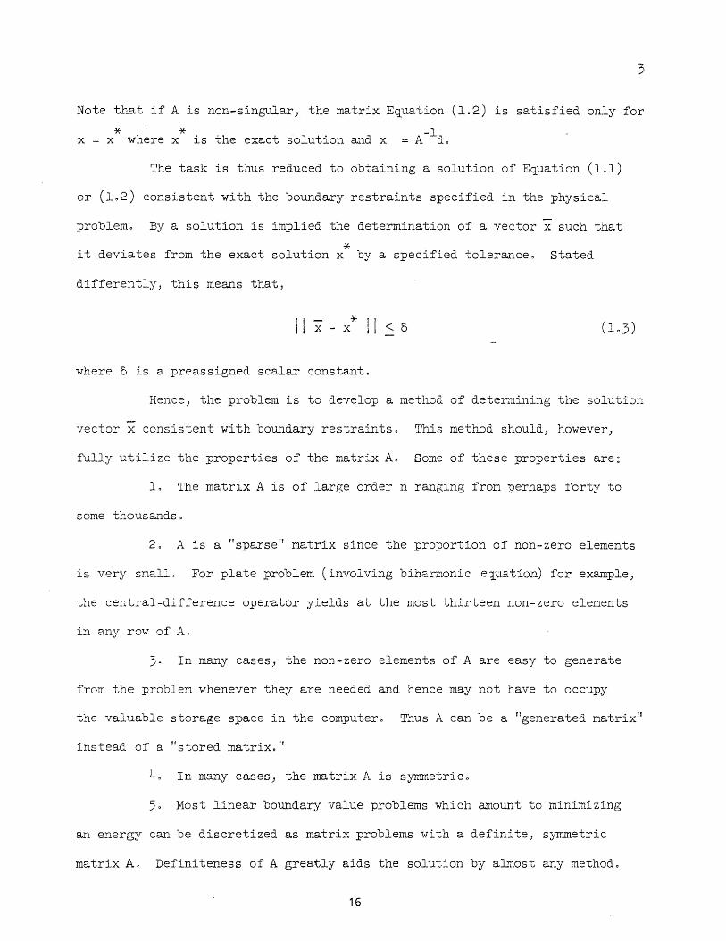
Then, equation (207) can be written in the form:

( v+1) (v) C ('v) x = x + r

Using (3.,1) and (302)) one can \{rite:

- cl

Therefore; ( v+l) (v) r = [I + AC] r' ,

Since A is nonsingu1ar (det A ~ 0)) one can rewrite (3.3) in the fOrTI~

-1 UsinG AHA = M)

., I .. \

= (AHA-.l.) r\.V) (Since H 1+ CA)

(v+l) (.~~.) r = Mr

(v) (v) To re1a~e the residual r with the error z ) write:

~­

Prenu1tiplyinC both sides by A) and substituting for Ax = d one gets

With this backgrolmd) (302) can be written in the form:

( v+k+1) (v+k) (v+k) x = x + Cr .

, ~(V+k) = x( v+k-l) + Cr (v+k-1)

Continuing)

30

l7

S b t Ot to ° 1 f (v+l) (v+2) (v+k) ° th fO t f u S l U lng succeSSlve yor x ) x oooooX In e -lrs 0

equations (3.2a)) one can rewrite it as:

x(v) + C [~ r(V+j)] ~i±O

But accordins to equation (3.5))

Therefore)

ContinuinG) r (v+k) = Mr(V+k-l) k (v) = Ivf~ r

f (v+k) (v+k.-l) SubstitutinG or r ) r (v+l) r in (3.7), one gets

= x(v) + C [~ Mj ] r(v) j=O

The above equation describes an acceleration procedure similar to the one

suggested by Hotelling7 (1943) in which)

1-,here: H = I + CA

If v = 2TI) this may be written as~

( ) 2 2m- l (0) x v = -(I + H) (I + H ).0 .. (1 + H )(Cd)+ HV x

If v is sufficiently larGe) r-{- 0 (since the process is assumed to be

convergent) and the last term in (3.10) may be neglected.

31

18

19

It should be noted) however) that in (3.9) and (3.10) one needs to

know M (or H) and its powerso This re~uirement is ~uite difficult to satisfy

since the matrix M (or H) and its powers have to be explicit~J formed) and

having done so, these have to be stored in a great deal of computer memory

space.

An equivalent formulation of (3.8) in terms of the characteristic

values and the characteristic vectors of M can be obtained by reference to

equation (3 n 5 )

in which the matrix M operates upon the residual rev) to yield r(v+l).

-1 Since the matrices M = AHA and H are similar, the characteristic values of

1 M are the same as those of H .

Assur.ring that the characteristic values f.... (j. = 1,2, •. ,11.) correspond l

to linear elementary divisors) one can uni~uely decompose rev) as~

n = L.

i=l b.p.

l l

where b. are scalar constants and p. are characteristic vectors of r1o. l l

Since by de fini tion M:p. = f.... P .) e~uation (305) can now be written as follows: l l l

(v+l) n r = L.

i=l

n = I:

i=l

32

b.Hp. 1. l

b.f....p. l l 1.

C:Jntinuing)

and in general)

k (v+j) The swn I, r in (3.7) j=O

k .L: r

j=O

r (v+j) n

I,

n .L: b.t-. '~J!.

i=l l 1 l

i=l

j b.t-.. 1'.

l l l

can then be vlri tten as:

(v+j) n 1;:

j L: I, b.l\.. p.

1=1 j=O l l l

After substitution from above) (3.7) reads)

n k . L: I,'b.I\..Jp .]

i=l j:;!O l l l

2 k +. 0 • • + b (1 +t-. +1\. +. . . • + I\. ) P ] n n n n n

TIle equation (3.14) describes a scheme to jump k cycles at a time.

However) it presumes a l~owledge of the characteristic values and character-

istic vectors of Mo

3.3 The Scheme

The acceleration schemes (3.8») (3.10) and (3.14) for advancing the

20

iterative sequence by k cycles at a time) have more or less no practical value

from a computational point of view. The schemes (3.8) and (3.10) require a

great deal of computational work to be done prior to mal(inc; the jump and this

feature mainly offsets the advantage gained by making the jump. Also) enough

33

2.1

memory space may not be availatle to store the matrix 1-'1 or H and its powers 0

The scheme (3014)) whenever applicable) is of theoretical interest only

because it presumes a lmowledge of f.... and p. (i = 1)2 .... n) of matrix M, l l

whose determination in itself is a more time-consuming task than that of

solving the system of eQuations (102)0

However) certain observations regarding the behavior of the residual

vector lead to a very useful approximation to the schemes (3.8) and ()014)0

The last equation in (305a) can be rewritten for v = 0 and k = m (m = 1)20.0~)

as:

r (m)

Here, the matrix M has a reducing effect on r(O)o

Assuming that the characteristic values f.... (i = l,2nnoon) of Mare l

real and that they correspond to linear elementary divisQrs) one can express:

(0) r =

where g. are scalar constants and p. are the characteristic vectors of M, l l

The eQuation (3015) then reads as:

r (m) n

L,

i=l

Since, by definition) :t-'Ip. l

t... . p .) l,·fp . = t.... ffip .) and. th(.:re fore l l l l l

r (m) n

= L,

i=l

m f,.f.... p.

l l l

Because the iteration (209) is assUlned to be convergent) the f.... (i l

are less than unity in moduluso Hence:

34

22.

1 > I~i! > !~ill >nQ.ooo> I~iml

(i = 1)20 n n "n) (3.18)

Thus) each component g.p. (i = 1)2nooon) of r(O) diminishes by a factor~. l l l

(i = 1)20.' on) after every cycle,. In this process) hm-lever) the Illower

components)1I i.e.) the components corresponding to the lower values of IA.. \) l

diminish more rapidly than the hieher ones. In fact the number of cycles

p required to reduce \A..PI to a small constant E) drops do"\{n exponentially l

as l~. I is reduced from illlity to zero. Figure 1 shows graphically the l

variation in p with respect to lA.il (0 ~ \A.il < 1) for E = 10-2

. 5) 10-5 ,

If~. are arranged such that: l

then in tne course of itera.tion) the conponents of r(O) cease to contribute

significantly towards reduction of the residual) in the order

g p ) g IP 1< ,. n',' ·glPl' After a certain stage of iteration "\{hich will n n n- n-

be called lIstable) II the component corresponding to the largest ~i) io ec.,

i\l) or the cOf.".ponents corresponding to a. group of the larGest i- _:) i" e 0 -'

~l) ~2' .. 00A,£ (l<n), predominate in the relation (3,,178.)0 This means

th -I- - TIl that after the stage of stability) each of e componenvs g,A, p. l l l

(i + 1 or i ~ 1,200'.£) in (3ol7a) will be negligible as comp~red to

glf...1

mpl

or G.f.. _::-'p. (j J J J

predominates) one CaJl approximate (3.17a.) as~

35

In the other case when a group of components g.A.mp. (j = 1)2 .... L) J J J

predominates) A. differ little from each other in absolute value and one J

can approximate:

A. = A J

i

( j

The relation (3.17a) can then be rewritten as:

1m g.A p.

J J

(m+l) ..., "\ ~ (m) r _ !'. r

In general) A differs from Al by a very small amount and in what follows a I

notation A will be used for both A and AI'

With this observation one can rewrite the expressions e3.20) and

(3.20a) for all v > mas:

Contin'Ji:-lG,.

and r (v)

k The S'....lr.. L

(v+j) r in equation (3.7) can then be approximated as:

l' _r',

v-I..-

k I.

j=O

k r ( v +j) : I. A j (v)

r j=O

The equation (3.7) now reads;

x(V+k+l) - xev) + C [~ Aj ] rev) (3.7a) j=O

I

vector X (v+k+l) l'n (3-7a) by x(v+k+l) ) Denoting the approximate _ one

finally gets:

36

( v+k+l) x r (v)

The eq'..1G.tion (3.23) outlines a jurap scheme which is essentially an approxi-

24

mation to those described by (3.8) and (,3,14). For its, use in practice however;

it is necessary to set up a procedure for evaluation f.. and for determininG the

staGe wl"len the i terati ve process becoGes stable. The basis for such a

procedure is available in equation (3.22):

(3·223.)

To evaluate f.. from this relation, the concept of u norm of 8. vectorll is qUi tc

usefu~. A ncrm r.:ay be introduced in different ways, and in different cases

one or 7,{lC other no1T.l will pro'.:e -:::'0 be most convenient., General.ly) the "non:

of a vector- x" is an associated non-neJuti ve nwnber !! x !! defined in onc of

? the followinG ways-:

1. Ii . I ; x 1'1 = !;\a:-: "j

i

2. . \ ! III x. + i .. + ... , v+ X (3 .. 2 11. ) \ , x . or) l c- n

I! ! 1111 [ I j2 ! j2 2

J 1/2

3· x = Xl + ~ +. < .... + x I n

Having ch~sen one of the norms defined in (3.24), the value of f..

is obtained from;

I ~ should be noted that A .3.5 dete:rr.lined from (3.25) i s always pas i ti ve s inc e

37

by definition) both I !r(v+l)l I and I !r(v)! I are non-negative. Thus) when

(3025) is used to detennine f...) it is implici t1y assumed that A. and -hence "'1 1

in (3.20) or f... in (3.20a)) is positive. If it is YJ),own 'a priori; that

"'lor f... is negative) f... can be determined from the relation:

To mark the stage \Olhen the i terati ve process becomes stable) one

may compare the values of "A. determined from (3025)) over a number of cycles

in succession. For example) the iterative process can be assumed to be

stable for all v > m) whenever the condition:

< n

is satisfied for a preassigned small constant ~,

The relations (3.25)) (3.26) and (3,27) outline a basis for the

practical use of the jump scheme (3023).

Some General remarks should be made regarding the frequency and

extent of raaJ::ing the jump" The jump scheme (3023) asswnes the re1ation

(3022a) to hold true rigorously and as a result after the jump) some of the

error components in x( v) are reduced while others may be mac;nified'J '111e

(1I+k+l) (v+k+l) vector x deviates from x . and the discrepancy increases with

an increase in value of k.) the number of cycles jumped at a timen In order

to avoid a possible build up of error) it is necessary to restrict the 'value

of kn Again) before making the next. jump) it is necessary to reduce the

error components which are magnified after the preceeding jump" This can

be achieved by making the jump at intervals of cycles.

38

CHAPTER 4

EV ALUATION OF THE JillIU' SCHEME

1!-.1 Introductory Remarks

In developing the jump scheme (3023)) two successive residual vectors

are assumed to satisfy the relation (3.22a)o As a result of this approximation)

the t ( v+k+l) bt· d ft th' d'ff f tl t (v+k+l) vec or x ) 0 alne a' er e Jump l ers rom 1e vec or x ,

which is the vector resulting from (k.,4,'1) iterations 'vithout jump) and the

difference is a measure of the approximation involved. It is the purpose of

this chapter to study the degree of approximation involved in the jump scheme

and to study the gain in convergence associated with it,

4.2 General Background

(v+k+l) In the jump scheme (3.23) one derives a vector x from a

given x(v) after one cycle of jump" Had the scheme ().23) been exact,

(v+k+l) ( v+k+l) x = x 0 From the point of vie'Yl of the residual) beginning with ,

( v) ,(v+k+l) r a new Tesldual r . is obtained after a cycle of jump such that:

(v+k+l~ r = Ax(V+k+l) - d

(v+k+l) where) x is givenhy (3.23).,

With an exact jump scheme) r(V+k+l)

(v+k+l) r

. ( V=l-k+l) I-lould equai T

( v+k+l) where, x is obtainedfTom-(3.l4 ).

(4.1)

such that,

If no jump is executed; that is) if ~ = 0 in (3.23), the iterative process

(2.1) would yield) after a cycle of iteration, the vector x(v+l) corresponding

26 39

27

to which, y(v+l) is:

( v+l) (v+k+l) (v+k+l) . The residual vectors r ) r and r form the startlng

point in studying effectiveress of the jump scheme (3.23). To appreciate this

fact) one can proceed thus:

From relations (3.5)) (3.12) and (3012b)) one has:

and

and

(v) r =

r (v+l)

(v+k+l) r

n ~ b.p.

. 1 l l l=

n ~ b.A..p.

i=l l l l

1.=1

n ,L: b .A.. k+lp .

l}, l

Using (401) and (402)) one can write;

Since from (3,23))

1 k ( v+k+ 1) _ ( v ) C [", "\ jJ ( v ) x - x + 6 I~ r

_i=O

(v) after substituting for r " from (305) one gets:

Also) from (3014),

Ink . ( v+k+l) (v) [ J ] x = x' + C ~ ~ b.A p.

. 1 . 0 l l J..= J=

X(V+k+l) = x(v) + c [~k j ] _ ~ b.f... p. i=l j=O l l l

40

(4,,4)

(406)

Hence) with x(V+k.+.l) and x(v+k+.l) from above) (405) reads as~

since AC = M-I, and Mp. = A.p. by definition, . l l l .

(v+k+.l) - r

n k. . . I: I: b. (.l-r... )(/10. J -A, J) p.

. l l' . l l i=l J=l

For a given (\ .. J it can be observed that) l

Denotins

A,( .l-A. k) (I-A. )

E~uation (4,7) can now be written as~

(v+k.+.l) Cv+k+l) n

It.. (l-t. k) - f.l(l-t. i ) ] Pi r - r' = I: b. i=l

l l' l

Since) (v+k.+l) n [t.k+1J . r' I: b. l Pl

i=.l l

One fina.l.ly gets~ (v+k+l) r' -

(v+k+l) (v+k.+l) Compare these expressions for r and r - wi th_,

41

2.8

(~-. 7)

(v+l) r'

f (v+l) (v+k+l) A close look at these expressions or r ) r

29

and r (V+k+l) 1 revea s

for a Si ven component b. p. of r ( v)) the follm'ling possibilities regarding the l l

effectiveness of the jump~

(a) the jwnp will be "over-effective;1! if:

(b) the jump will be flfully effective)!! if~

I ~. - f.L (l-~.) l l

(c) the jwnp vill be Ifparti.ally effective) II if~

1 A, • k +11 < I A,. - ( .l-~ . ) 1 < 1/1.. I . l . . l f.L l 1 l'

(d) the jump will be of no advantage if~

11\ .. i • l'

(4., .lOd)

and finally)

(e) the jur.:p will be "negatively effective)" i 0 e,,) the error will increase if·;

The tenT lrei'~ective" in the above statements should be interpreted with the

purpose of the jump in mind) which is to advance the iterative sequence by

k cycles beyond (v + l)th iteration.

Since the conditions (l~vlOa)b)c)d)e) are only qua.litative statements)

it is necessary to develop quantitative measures to study the effectiveness

42

30

of the jump scheme (3.23) ,. However) from these conditions one can determine

bounds on jJ. for the jump to be positively effective or otherwise ..

Referring to (4.108..;'0) and c) it can be observed that the jump will

be positively effective) if and only if:

! 1--.. - jJ. (l-~.) I < ! I--. . I 1 l 1

(4011)

In this connection) there are four possible combinations of 1--.. and jJ.) which 1

can be stated as follows:

(a) A. positive) jJ. positive 1

(b) 1--.. neG~tive) 11 negative 1 (4012)

(c) t... positive) \.l negative 1

(d) 1--.. ne[;ative) jJ. positive 1

Hote that jJ. is :positive if and only ':..JO' "\ .J...L I'. 15 positive) and f..l is

negative if and only if t.. is negative) and conversely.

To study each combination individually) one can proceed thus~

(a) If~. and jJ. are both positive) a necessary and sufficient 1

condi~ic~ C~ ~ to satisfy (4.11) is:

2A. O < < __ 1_

jJ. 1-1--.. 1

7":-.::'5 implies that for the jump to be of any advantage) jJ. and hence

I--. r:rus"t be ;-:;s:' -:l 'te 0 Also for jJ. = 0 or jJ. = 2A ./I-A.) the jump does not have l' 1

adv ant 8.[; c c~\rer the normal iterative sequence) and for all 1-1, > ~. /l-~.) the l' 1

jump is ne=at:vely effective.

(0) I f both t... and ~l are negative) the condition (4.11) will be 1

satisfied if and only if:

43

any

Thus, for the jur.lp to be positively effective) ~ and therefore A.

mus t be negative. Also for ~ o and ~ = 2A. /l-A. .} thc junp does not offer 1 1

any advantage over the nonnal i terati ve scquence) and for all ~ < 2A. /l-A.. ) l 1

the jump is negatively effective.

(c) If A.. is positive and ~ negative) the factor ~(l-A..) in 1 . 1

(4.11) is always nesative and thercfore the condition (4 .. 11) can neYcr bc

satisfied. Hence) the jump in this case is always necati vel:), effective.

(d) If A.. is negative and ~ positive) the· factor Il(l-;....) is , 1 1

always positive a:.nd .. therefore the condition (4,,11) can never be satisfiecl.

Hence) the jump is always neGatively effective in this case.

From this 'discussion) one can conclude the followinc for a Given

(v) conponent b.p. of r : 1 1

Condition [4.14.1): The jump can be positivcly effective i1' and only if)

~i and Il are of the same siG~} and whenever it is so) the jurr~ will be

positively effective if and only if}

31

( 4.1ho.)

Condition [4 .1LL 2) : Whenever t.., and ~ are of thc SBJile sign., no aclvanta3e l

(fron convercence point of view) is ~ained by jUl~1pinG) for

2A. 1

l-A. . 1

Condi tion [4. 1 1l-. 3] : Whenever Ai a.nd ~ are of the S8J:J.e sign) the jump will

be necatively effective if and only if}

44

2A. 1

1-"-, 1

(4u14c)

32

If both~. and ~ are positive) the inequality (4014a) can be rewritten l

in terms of ~ as~

Since)

r... > ~ l ~+2

+"\2 3 k

= A, I\, + f.. + 0 " .' 0 + f.. .'

and since 0 < f.. < 1) one can write for a given k)

Therefore for all :positive ~;

Lim ~ - k: r..-l

one can restate the condition [4~1401J as~

(4015a)

Condition [4.15.11: If 1\. and 1\, a.re both positive) the jump will be positi.vely l

effective for all f..i > /\'cr} where /\'cr = k/k.+2o

When A. and ~ are both neGative) the inequality (4.l4a.) can be l

YCiJri tten in teIT.1S of ~ as:

(4.15b)

In this case) the limits for ~ are given by~

and no useful bounds for ~l/~Li-2 are available. Hence) the condition [4oll~"lJ

can be restated as~

45

33

If A. and A are both negative) the jump will be positively l

effective for all A. < ~/~+2u l

With this general background) an analysis of loss and gain associated

with the jump scheme (3023) is presented in the following sectionso

403 Loss and Gain Analysis

It is the purpose of this section to present a systematic procedure

for evaluating quantitatively the effectiveness of the jump scheme (3.23)

which aims at advancing the iterative sequence by k cycles at a time 0 Because

of the assumptions introduced in its derivation) the scheme (3.23) is

approximate in nature and consequently it is very essential to study the

effects of approximation on the convergence of the iterative sequence 0

In the preceeding section, conditions are derived stating the limits

for ~ and A. to determine qua1itatively) whether the jump is positive1y l

effective or otherwise for a. given component of the residual 0 They do not

provide ~~y information regarding the degree of effectiveness of the jump 0

This aspect of the problem is discussed below 0

Th . -P.l..(",'Y' r( v+l) and r( v+k.+1) i) . e expresslons J.L

r (v+1)

(v+k+l) r

n L.

i=l b. [A. J p. l l· l

n L.

i=l b. [A. - ~ (I-A.) ] p.

l l l l

play an i~portant role in the loss and gain analysis of the jump scheme (3023)0

This happens because by definition) the term effectiveness of the jump is

interpreted in connection with the state of iteration at (v + l)th cycleo

If one rewrites (409) in the form:

46

where;1

(v+k+l) r

e. l

i n 2:

i=l b.A..

l l [e.] p.

l l

A. - tJ. (l-A. ) l l

r.... l

(4018)

then) the magnitude of e. for a given fl indicates the extent to which the jump l

f (v+l) modifies the component b.t..,.p. 0 r . Thus the jump is positively effective

l l l

Ie. 1 < 1 l

and the jump is negatively effective if)

Ie. 1 > 1 l

(4020b)

Conditions (4.20a) and (4020b) lead to two distinct possibilities

which should be discussed individually~

Case A; for Ie. I > 1) loss analysis. l

Case B: for Ie. I < 1) gain analysiso l

However the discussion of case A and case B should be preceeded by a study

of the general behavior of e. as a function of flo Four possible variations l

in this connection) with 0 < !A. I < 1) are~ - l

10 f... positive andt.., positive l

20 A. negative and A. positive l

30 f... positive and A negative l

40 f... negative and f.. negative l

Rewriting) A.. - tJ. (l-A. ) e. l l

l f... l

(l+fl ) - 1 f...

l

47

(0 < tJ. < k)

(0 < tJ. < k) (4.21)

(-1 < tJ. < 0)

(-1 < fl < 0)

(4.19)

(4019a )

35

one can proceed as follows:

10 If~. and ~ are both positive) ~/~. > ~ and therefore in (4.19a)J l l

as ~ increases from ~ = 0 to ~ < k) e. decreases in the order: l

e. l

(4021a)

2. If ~i is negative and ~ positive) ~/~i is always negative and

therefore in (4.19a)) as ~ increases from ~ = 0 to ~ < k) e. increases in the l

sequence;

e. = +1) +2) + 3 non 0 0 0 l

(4.21b)

30 If ~i is positive and ~ negative) the factor ~(l-~i) in (4019)

is always negative and therefore as ~ decreases from ~ = 0 to ~ > -1) e. l

increases in the order~

e. l

(40 21c)

4. If both ~i and ~ are negative) the factor ~(l-~i) in (4019)

is always negative and therefore as ~ decreases from ~ = 0 to ~ < -1) e. 1.

decreases in the sequence~

e. l

+ 1 ) 0., -1) - 2 } - 3 0 0 0 n 0 0 (4. 2~ld)

With this preparation). a detailed discussion of case A and case B follows

under the respective titles) "Loss Analysis" and "Gain Ana.lysis 0 11

40301 Loss Analysis

(v+k+l) d (v+l) Referring to the expressions for residuals r an r )

(v+k+l) r

n 2::

i=l

48

b.~. [e.J p. l l l l

(4018)

where e.

l

(v+l) r

tv. - ~ (l-A. ) 1. ' 1

A.

n L:

i=1

1

b.A..p. 1 1 1

6 .3

one can observe that corresponding to each Ie. I > 1) the jump is negatively 1

effective for the component b.p. of r(v). The magnitude of e. indicates the 1 1 1

extent to which the jump magnifies the component b.A..p. of r(v+l) with whi.ch 111

comparison is made for effectiveness. Also) this iJnplies a IllosS'1 for the

i th residual component) because some additional iterations are re~uired to 9

(v+k+l) reduce b.A.e.p, of r by a factor e.. Since the jump scheme (3023) 1 1 1 1 1

expresses the gain in terms of numbe.r of cycles jumped beyond the (v + l)th

iteration) it is appropriate and consistent to specify as a measure of loss)

the number of additional iterations ill) re~uired after the jump to reduce the

I I .. (v+k+l) (v+l) component b.~. e. p. of y' to its counterpart b.A..p. of r 0 1111 111

Since after every cycle of iteration) each component of the residual is

multiplied by the corresponding value of A.) the value of m is such) that 1.

A.m le.1 = +1

1 . 1

To derive an expression for m from e~uation (4022)) it is necessary to study

individually the four cases specified in (4,21)0 One can proceed as follows~

1. If both A.. and A are posi.tive, according to condition [40l501J 1 '

the jump is neGatively effective whenever ~.< A. 0 In this case, according 1 cr

to (l~~21a)) e. < - 1) and therefore (4,22) can be written as~ 1

49

Substituting for B. from (4019)) one can write l

m-1 /I..

l

1 ~ (1-A. . ) -A..

l l

Taking 10garitlnn of both sides and rearranging terms) one gets

m 10[:;[11 ( 1-A. . ) -A.. ]

1 _ __~--=-::--l-=-_l log [A.~: ]

l

2. If /I.. is negative and A. positive) according to condition l

[l~ol4~1J the jump is always negatively effective. In this case) (4021b)

Gives

Since

B. > + 1 and (4022) can be expressed as; l

A. is neGative and 8. l l

A..m e. = + .1

l l

positive) ill must be eVen

( -A. . )0-1 A.. ill-1 Substituting for e. from (4019)

l l l

1

&'1.d therefore)

one gets~

Taki:1C 1::.:;8.:'':'' ~~:::: of both sides and rearrangine; terms) one can write

7 "'.

m 1 - log r -A.. OJ ... l-'

If A.. is positive and A. neGative) according to condition l

[4.1l.;..~: -..::c: ,-'" .. ::::p is alvays negatively effective. In this case) (4021c)

gi ~les e" > + :. 8...'1d one can rcwTite (4.22) as: l

"A,.nlB. +1 l l

After substitution for e. from (4.19) this reads as: l

50

37

Taking logarithm of both sides and rearranging terms) one can express~

log[l-.. - 1-1(1-r-".)'1 l l -

m=l------::---,::----log(/-... J

l

A bound for the value of m in (L~ 0 22c) can be determined as follows:

With positive 1-.. (0 < 1-.. < 1) and neGative 1-1 (-1 < 1-1 < oL one can observe l - l

that)

and) - I-l ( 1-1-. .) < (l-~.)

l l

Therefore) -r-.. - 1-1(1-1\.) < 1

l l

and) - 1 < lor: r.-r-.. - 1-1 ('l-A, . ) J < log [r-". ] < 0

~ l l' l

Hence) log[l-.. - l-1(l-~.)J o < l l < + 1

log [f-". : l-

This leads to the conclusion that whenever ~. is positive and I-. nesative) l

m < 1 (4.23)

4. If both I-.~ and /\ are negative) according to condition [401502J ..L.

the jump is negatively effective whenever ~. > 1-1/1-1+2. Then) (4,21d) gives l '

e < - 1 and (4.22) can be revTritten as ~ i

51

39

Since both A.. and 8. are negative) m must be even and therefore) l l

( _ '\. )m-l = _ '\ .m-1 o b·.J..· 8 f (' 4 19) -I-1\0 I.... Su stl L"utj nc; for . rom 0 one rz.e vS , l l l ~ .

(-A,. )m-l l

1 A.. - 1-l(1-A..)

l 1,

Taking logarithm of both sides and rearranging terms) one can express:

m 1· log[A. - l-l(l-A.) ]

J l

lag [.-Ai. ]

( 4022d)

A bound for the value of m in (L~o 22d) can be determined- as follows:

Wi th nec;ati ve Ai (-1 < Ai ~ 0) and 'negative I-l (-1 < I-l < 0)) one can observe

that:

- 1-l(1-A..) < (1-A..) l 1.'

Therefore) A. - II ( l-A. .) < + .l l ,..... l'

(h,,24b)

- !J,Cl-7\,.) > - 2A. l l

Then) A.. - I-l ( l-A, .) > - A..

l . l l

Hence) from (4 0 24b) and (4024d) one derives~

- 1 < 10D" [A.. - ~L ( l-A . ) ] < log [ -f". ] < 0 U l . l l

( 4.,24e)

Therefore) log [r... - I-l ( l-A, . ) J o < l l < 1

log [-t..,. ] l

(402.4f)

This leads to the conclusion that if both r... and A. are negative) the jump l

52

is negati vely effective "Ylhenever r... > 1-1/1-1+2, and then) l

m < 1

40

In concluding loss analysis of the jump scheme (3 23), two observations

can be made as follows:

Condition [402201J~ The loss in number of cycles m is in 8eneral a function

of A.) A. and k - the number of cycles jumped ·at a time 0 l

Condition [4.2202J: The value of m is less than unity whenever A is negative.

4.302 Gain Analysis

( v+k+l) Reference to expressions (ILlS) and (3012.) for the residuals r

and r(v+l) respectively, SUG8ests that the jump is positively effective for

the component b.p. of r(v) only if? lB. I < In The maGnitude of B. is l l . • l l

indicative of the deGree of reduction of the cor.lponent b.A.p. of r(v+l) l l l

and if B. = 0) the jump comp1etely eliminates the i. th component of the l

resiclualo

Consistent with the loss analysis) it is proper to specify as a

measure of Gain the number of cycles ill., that would have been necessary after

(v+l) the (v + l)th iteration to reduce the component b.A.p. of r by a l l l

factor lB~ I. Then, m is such that it satisfies the relation, -l.

.Accordins to condition [401401], the jump can be positively effective if and

only if A~ and 1-1 are of the same signa In this connection there are two

distinct possibilities:

1 0 pos i ti ve A,. (0 < A. < + 1) and po s i ti ve 1-1 (0 < 1-1 < Ie) l - l.

2 a negative A,. (-1 < A. < 0) and negative 1-1 (-1 < 1-1 < 0) l l -

A discussion of each of these possibilities is given belowo

53

10 If both 'A.. and iJ. are positive) the jum.p is positively effecti.ve l

whenever)

21-.. l

o < iJ. < I-f-.. l

Referring to the expression (4.19) for G.) l

e. l

"A.. - iJ.(1-~.) l l

"A.. l

one can observe that e. decreases from e. = +1 to e. = -1 as iJ. changes from l l l

iJ. = 0 to ~ = 2I-.i/l-~i 0 To determine the value of m from (4.25) _, t;wo ranges

of iJ. should be considered separately as:

W.l

( a)

(b)

o < iJ. ~ ~i/l-'A.i) corresponding to which Gi is positive (0 ~ Gi < + 1).

'A../l-f-.. < iJ. < 21-../1-;....) corresponding to which e. is negativE:: l l l' l l

(-1 < e. < 0) 0

l

Positive G. l

( 0 < iJ. < 'A../l-'A..)~ In this case) the enuation (4~25) can be - l l' ':1.

written as

,.m e I'. +.

l l

Substi tutinc; for e. from (L~ 0 19) and tal~ing logarithm of both sides) one gets l

after rearranging terms)

(4 25a)

(~./l-~. < f.l. < 2A./l-t...): Equation (4.25) can be \'[ritten in l l l l

this case as)

Substituting for ei from (4.19) and taking 1oe;arithm of both sides) one can

write after rearranging terms y

54

_ log[!J.(l~~i) - t-. i ] m= --.------.-.- - 1

log [I-.. ] 1

2. If 1-.. and !J. are both negative) the jump is positively effective 1

whenever)

Referring to the expression (4.19) for e.) one can note that e. decreases 1 .1

from e. = + 1 to e. = - 1 as !-l c hanee s from !J. = 0 to !J. = 2f... 11-t-. . a To find 1 1 ; 1 1

42.

the value of ill from (4.25) two ranges of !J. should be c~nsidered separately as:

( a)

(b)

I-../l-~. < !J. < 0) corresponding to which e. is positive (0 < e. < + 1). 1 1 - 1 - 1

2f.../l-~. <!J. < I-../l-~.) corresponding to which e. is negative 1 1 1 1 1

(-1 < e. < 0). 1

Positive e. 1

(~./1-~. < !J. < 0): In this case) the equation (4.25) reads as: 1 1 -

~.m + e. 1 1

Since I-.i

is negative and A.im positive) ~iill = (-~i)mo Now) substituting for

e. from (4.19)) one gets) 1

f.l(1-~.) - ~. ( _A..)ill = 1 1

1 ( -~. ) 1

Tru~ing logarithm of both sides and rearranging terms) one can write~

Negative e. 1

this cas e as:

10G[!J.(1-~.] - 'A.J ill = _________ l~~--l_ - 1

log [-A. J 1.

(2f... 11-1-.. < !J. < ~. II-A.. ) ~ Equation (4.25) can be \.,rri tten in 1 1 l' 1

55

SInce A. i is negative and (-6 i ) positive) A,im

is posi.tive and therefore

;.... m (-A.. )m 0 Then, substituting for 6. from (4n 19)., one gets) l l l

A.. - ~L (1-/1.. ) ( -A, . )m = l ( l

l -A,. ) l

Taking logarithm of both sides and rearranging terms) one can write~

m = log [A. - ~ ( l-A.. ) ] ___ l ____ l ___ 1

[-;.... 'J l'

In concluding gain analysis of the jmnp scheme ~ .3.2.3 L two observations

can be made:

Condition [L~.25"lJ: The number of cycles m) gained beyond the (v+l)th

iteration is in general a function of A..) A, and k - the number of cycles l

jumped at a time.

Condition [4025n2J~ The number of cycles gained is infinite) ioe" the

jump completely eliminates the i th component of the residual) whenever

6. 0) ioe. whenever ~ = A../I-A,. OT in terms of Ii) whenever A,. = ~/'''+lo l 1: l r- l r-

404 N~erical study of Variables

With expressions available to evaluate the loss and gain associated

with -the jw":1}l scheme) it is now proper to make a numerical study of the

relationship among the variables involved 0 The purpose of such a study

would be:

1. To determine the optimum frequency and extent of the jump;

that is) to select the interval in number of cycles between two successive

jumps and to choose the value of k, the number of cycles jumped at a time.

2. To study the effect of jump on the reduction of residual

components 0

56

The fre~uency of jump depends upon the magnitude of maximum loss

associated with the jump) which in turn is a function of k) the nUmber of

cycles jumped at a time. The problems of determining the extent and

fre~uency of jump are thus interrelated.

The interval between two successive jumps should be at least e~ual

to m ) the maximum loss associated with the jump. This would assure that max

no component of the residual is cumulatively magnified in the course of

iterative process. Also) some additional cycles are re~uired so that these

magnified components of the residual are reduced at a rate similar to that

of the others. The selection of k-is based on two considerationso In the

first place) for a given A) the maximum loss increases with k) and hence

the optinur~ interval between two successive jumps is increased. Secondly)

for a larGe k) the factor ~L is large and hence the difference between , (v+k+l) (v) x. and x. increases with increasing ko TIllS might introduce

l l

excessive round-off errors if k is too large~ With this introduction) one

can proceed with a numerical study of the variables involved in loss and

gai~ anal::s is,

':'::e variables introduced in the loss and gain analysis of the

jUT.1p s:~e:::e a~e:

A. (i :: :..2, ..•. n !'and 0 < \A. I < 1)) the characteristic values of matrix Hj l l

A (0 Sit. \ < l), the ratio of two successive residual norms and

k) the nUDber of cycles jumped at a timeo

In the e~~ressions for loss and gain) both A and k enter as a

single variable ~) where ~ k .

1\(1-/\ )/(1-"-) 0 The range of ~ is) 0 <: ~ < k

for positive 1\ and ~ 1 < ~ < 0 for negative /\. For positive 1\) the

57

of I\. 0

k. Figure 2 shows for k. 10., the variation in fl as a function

To appreciate the role played by 1\.. in the reduction of residual) l

values of 1\.. P are tabulated for p = 5,9 10 and 20 in Table 10 These values l

indicate the rate at which eve~J component of the residual is diminished in

the process of iteration.

4,4.1 Loss Analysis

Since for negative A) the maximum loss m is bounded by TIl = 1) max

only cases involving positive t-. are of interest ion this studyo These are)

(a) positive 1\.. and positive A) and (b) negative~. and positive 1\.0 l l

(a) In this case) the residual components corresponding to

1\,. < fl/fl+2 are magnified after the jump) and then the loss m is given by l

( 40 22a) 0 For a given k) m increases with increasing l-L and therefore) the

maximum loss is obtained when 1-1, = ko Values of m are tabulated (in Table 5a)

and plotted (in Figure 3) for I\,i < k/k+2) and for fl = k.) with k = 5) 10 and 20.

The naximum loss in number of cycles is" m = 2,1 4 and 7 for k = 5) 10 and max

20 respectivelyo

(b) With negative I\,i and positive 1\", the ju.mp is always negatively

effective and the loss m is given by (4022b)o In this case] m increases

wi th increasing f.l for a given "'i ·iand then) the maximum value of m is obtained

for ~ = k. A~ain, for a given f.l, m increases with increasing !~il) and

for 11\..\ = 1) . l

m - 00 - 0 The Table 5b gives the values of ill for - 1 < 1\,. < 0)

l

and for f.l = k with k = 5, 10 and 200 These values are plotted in Figure 3

showing the variation of m with respect to t-.. 0 Since for all fl > 0., m ~ 00 l

as /-...-- -1) the maximum loss is a function of both k and the largest l

absolute value of negative t-.. 0 However unlike in the previous case) the l

magnitude of (-/-...) plays a major role in the build-up of erroro lomax

58

46

~lUS) when a positive ~ is used) the interval between two successive

jumps is determined by two factors~ (1) If all ~i (i = 1;2o~oon)- are positive;

the value of k controls the frequency; eogo; for k = 5) 10 and 20; the interval

should be at least equal to the maximum possible loss) which is 2; 4 and 7

cycles respectivelyo (2) If some ~. are negative) both k and value of (-~.) 1 1 max

control the frequencyo Reference to the Table 5b shows that as lA,i.! approa.ches

unity) ill increases very rapidly and beyond some value of l~.!) the magnitude 1

of loss is so large that for a frequency of jump based on its consideration"

the jump scheme (3023) looses its importance as an acceleration procedureo

Thus} it is necessary either to restrict the value n~ (-A) . o __ r t_o ha_ve a ,- - - '. . -i .r max.l - -

procedure to control partially or completely the excessive loss associated

with the jump" The latter consideration is discussed in detail after a

numerical study of the gain of the jump scheme 0

When a negative A. is used) the maximUlTI loss is only one cycle) and

hence the interval between two successi.ve jumps can be as smal.1 as one cycle 0

40402 Gain Analysis

In this connection J a, value of k = 10 is used to study numerical.ly

the relationship among variables A,. and A,o Since the jump is positively 1

effective only when 'A.. and ~ are of the same sign) two possibilities arise 1

in this connection~ (a) both~. and A, positive) and (b) both~. and A. 1 1

negative 0

(a) In this case) the jump is positively effective for all

~. > ~/~+2 and then) the gain ill is equal to k cycles for t..,. =!\, 0 The 1 1

':fable 6a gives the values of m indicating the extent of loss and gain in

number of cycles for k = 100 The Figure 4 shows graphical.1y the variation

of m with respect to~. for k 10 and for ~ = 007) 008) 009., 0095 and 00990 1

For a given 1-1) the component of the residual corresponding to A,. = A, = 1-1/~+1 1

59

vanishes, that is m = Co" and this is shown in the figure by a dotted vertical

line. However for a given k, the maximum~. corresponding to which the l

residual component vanishes is given by A. = ~ = k/k+l. This means that for l

k = 10) no component of the residual corresponding to t.... > 0090909 can be l

eJiminated by the jump 0

When f... and t... are both negative) the jump is positively l

effective for all Ai < ~/~+,2) and then the gain m is k cycles for Ai = Ao

Table 6b Gives the values of m for k = 10. Figure 5 shows graphically the

variation of ill with respect to t... i -? for k 10 and for A.-- = -004) -005., -006)

-007) -008 and -0.90 Observe that -for a given ~J the component of the

residual corresponding to A. = ~ = ~/~+l vanishes) that is ill = 00, and this l

is shown in Figure 5 by a dotted vertical linea However) in this case it

is possible to eliminate the residual component corresponding to any t...'J l

since the fl required for this purpose (fl = l\,i/1-t...i) 1i.es in the range

-1 < ~ < 00

An important observation can be made for the case when f.. is

neBa ti ve" Instead of advancing the i terati ve sequence by k c:,rcles at a

time) it is more advantageous to eliminate the maximum component of the

( k)i- ) residual after every jump) i 0 e 0 instead of having fl = A l-t... ! (I-I\, .' one

may use ~ = (-.../1-1\,0 This procedure can also be used for removing components

of the :-csidual corresponding to a particular value of t....) when some t.... l 1.

are negative and introduce large magnitudes of error in conjunction with

a positive value of flo

With this numerical study., the jump scheme (3023) can be modified

in some cases to give a faster convergence 0 This modification is discussed

in Section 4050

60

405 Modified Jump Scheme

In developing the jump scheme (3.23); it is assumed that the

iteration (209) has become tr s tablell in the sense implied by (3027)) and on

this presunwtion) the approximate relation (3022a) between two successive

residual vectors is derivedo The effects of this presumption are studied in

TIle study of loss and gain associated with the jump scheme (3023)

leads to a modification which consists in ignoring the requirement regarding

stability of the iteration (209) and thus using the jump~cheme (3023) from

the initial stage of iterative sequence. The different conditions under

which this modification applies) are:

10 If all f.... (i = 1)2oooon) are positive) the maximum loss l

associated with a jump is bounded and is of such a magnitude as to allow

a small interval between two successive jumps 0 For example) with k = 10)

the maximum loss is m = 4 and an interval of five cycles is sufficiento max

20 If some f.... are negative) but the magnitude of the smallest l

negative f.... is such as to allow a reasonably small interval between two l

successive jumps) then the modified scheme can be usedo For example) for

k = 10) and with (-f....) =" Q..,r7", the maximwn loss is m l ma.."'{ max

interval of ten cycles is sufficiento

If some f.... are negative) and if the magnitude of the smallest l

negative f.... is known) the modified scheme can still be usedo In this case) l

however) it is necessary to eliminate the components of the residual r(O)

corresponding to the smallest negative f....) usin~ 1-1 l

beginning of the iterative sequence.

61

f... . /1-).... in the l l

48

CHAPTER 5

EXPERIMENTS WITH THE JUMP SCHEME

501 Introductory Remarks

This chapter presents some experimental results with the use of the

jump scheme in conjunction with successive over-relaxa.tion (S.O.R~) method) for

solving problems of plates on elastic foundation. The S.O.R. method is selected

because of its applicability to solving the particular problem and because it

satisfies most of the requirements of the jump scheme (3023) and its modification

outlined in Section 4.50 The problem_of plates on elastic foundation was studied

for different boundary conditions and for different foundation cha.racteristicsu

502 The Method of Successive Over-Relaxation

where ~

and)

The partial differential equation for a plate on elastic foundation is,

q(XJY) N

a is the foundation constant)

N is the plate stiffness)

q(x,y) is the externally applied load

z is the deflection~

It is difficult to show conclusively whether or not the matrix corresponding to

the finite difference equations of (501) possesses "property (A)" as defined

in [20404Jo However) this can be inferred from the fact that)

10 the matrix resulting from the finite difference representation

of Laplace 7 s equation possesses "property (A)., II and

2 0 '~he So 0 oR n method converges when applied to the finite difference

62

50

For matrices having the "property (A))" certain observations can be

made regarding the characteristic values ~i (i = 1)2 .. ~.n) of matrix H(w) in

equation (2.30). Corresponding to every matrix A in (1.2) which possesses th~

"property (AL rr th~re exists a value w = wb

'

2

(where ~l is the largest characteristic value of H(l)) such that for all

4 w < wb ' the following holds true •

The values ~i (i = 1)2 .... n) can be divided into three distinct

groups) such that: (a) some ~i are positive and distinct) and are all greater

than (w-IL (b) some ~i are negative and are all eClual to -(w-l), and (c) some

~i are complex and distinct) all havinB the modulus less than (w-l)o

In order to study the jump scheme in conjunction with the S.O.R.

method) the value-of w was restricted to the range 1 < W < wb ) since for all

W > wb the ~i (i = l,2.o.,n) are all complex with eClual modulus which is

(w-l). Also) a few cycles (v=20) were run in the beginning without jump) so

that the components of residual' corresponding to the complex and negative~. l

are reduced significantly before the junp scheme is introduced,

In connection with the S.O.R. method) the jump scheme (3·,23) was

incorporated in the computation as follows: Having computed the factqr

~ j (v+k+l) (v) ~ ~ = (l~)J the set of values x are derived from the vector x ,

j=O r

in the sequence:

1. (v) Compute x ,using equation (2.24) with (v-l) replaced by v, r

and v by (v+l).

v - (v+l).

2. Compute x (v+l) using equation (2u25) with (v-l) = v and r

63

3· I

(v+k+l) Then) compute x from: r

(v+k+l) x r

,

Equation (5.3) represents the actual jump of k cycles. i

( -, -.."

51

4. C!t"'-yo~ v \V+K+.L) ....... \.J...L '- .il~r Repeat the steps

5.3 A Special Result

As remarked in the previous section) in the case of matrices having

the "property (A))" some of the /1... are negative and they are all equal to l

-(W-l). Before proceeding with the iterative sequence) it is possible in

this case to eliminate from r(O)) the components corresponding to these

negative ~.. This can be achieved by executing one cycle of jump with l

~ = A./l-A.) that is) using l l

-(w-l) I + (W-l)

w-l =~

W

The jur.'ip c8e:.fic::"ent can then be expressed as~

1 + ~ l-w

I +-­W

1 W

(v+k+l) SubstitutinG for (l~) from above in equation (5.3)) one obtains for x r

(v+k+l) x

r

~

64

(v+l) x r

Since x (v+l) r

is available at every stage of iteration) the procedure for

removing the residual components corresponding to the negative f.... -does not l

involve any additional computation.

Table 8 compares the residuals obtained by using equation (5.6)

once) with those using the SoO.R. method without jump.

5.4 Discussion of Results

The problem of plates on elastic foundation was solved by using

finite difference approximation (with central difference formula) to

52

equation (5.1)0 Square plates were studied with) (a) three types of boundary

conditions such that) all edges are either simply-supported) fixed or free;

(b) six different foundation constants a; and (c) three types of loading

conditions. A plate was divided into a 20 x 20 mesh) thus leading to

361 equations in the case of plates with s.imply-supported or fixed edges)

and to 441 equations in the case of plates with all edges free.

Because of a large number of equations encountered in the problem)

it seer.1ed a.dvantageous with respect to obtaining solutions to have as x(O))

the vector derived by interpolating results from a similar plate with a

10 x 10 mesha The interpolation was done using Taylor:s formula in

2-dimensionso It should be noted that the previous observations regarding

the jump scheme and the SoO.Rn method hold true for any arbitrary initial

approxi:r:mtion x(O). However) in some cases) the effect of using two

different initial vectors x(O) was studied with the other approximation

x(O) = O.

Different combinations of boundary conditions) foundation

constants and the type of loading were studied employing the SoOaRo method

with and without jump. As rema.rked earlier) the modified jump scheme was

65

53

used after first 20 cycles of iteration. The jump was ma.de at intervals of

10 cycles using positive A.) with k = 9. In general) the effect of the jump

was uniform) and a consistent pattern was observed regarding the reduction

of the residual. The jump was almost fully-effective as judged from the

comparison with the residual norms (Ir. (v)\ ) obtained without jump 0

l max

To indicate the effectiveness of the jump scheme) results are

presented for a typical case in Tables 7aa~d 7b. These results give the

values of the residual norm computed every 10 cycles) for first 200 cycles

-of iteration. In each table) two sets of values are presented; one

obtained with jump and the other without jump. The results in Table 7a

were derived for the initial vector x(O) = 0) while those in Table 7b

were obtained by using the interpolated vector as an initial approximation.

A comparison between these values would indicate the advantages of ha.ving

the interpolated vector for x(O). Observe that, not only are the residual

norms smaller in Table 7b than the corresponding values in Table 7a) but

also) the ratio A.IO between their consecutive va1ues is sma.ller. This

suggests that in Case [b) some of the higher components of the residual

are absent) and therefore the rate of convergence is higher than that in

Case 7a.

The values in Tables 7a and 7b indicate beyond rulY doubt) the

usefulness of the jump scheme.

66

6.1 Summary of the Study

CHAPTER 6

SilllMARY AND CONCLUSIONS

This thesis deals with the problem of solving partial difference

equations of elliptic tJ~e by certain iterative methods. A procedure is

developed to accelerate the convergence of explicit; linear iterative

processes of first degree. The procedure is called the "Jw-np Scheme" and

is intended to be used intermittently in conjunction 'vi th the pertinent

group of iterative methods. The name "Jump Scheme" is-quite descriptive

of the purpose of the scheme which is to jump or advance the iterative

sequence by a number of cycles in a single iterationo Tne concept of

acceleration implied here is thus similar to the one expressed in

Hotellinc's matrix squaring procedure7o Chapter 3 presents the basis

for the jQ~P scheme) and outlines the assumptions accompanying its

derivation. General remarks are also made for its use in practiceo

Certain simplifying assumptions are made in the derivation of

the scheme and as a result) some of the residual (or error) components

are reduced while the others are magnified after the jump. These effects

are identified respectively as IIloss" and Ifgain" associa.ted with the

jump scheme. The loss is measured in terms of the additional nUflber of

cycles necessary to reduce the magnified component of the residual to

its "would have been" magnitude in absence of any jump 0 Similarly) the

gain is expressed in terms of the number of cycles that would have been

necessary to reduce the residual component to its magnitude after the

jump. A detailed analysis of loss and gain associated with the jump

sche~e is presented in Chapter L~. Expressions to evaluate the loss and

67

gain in number of cycles) are derived and in certain cases) simple upper

bounds are determined for the loss associated with the jump. This is

followed by a numerical study of the variables involved in the loss and

gain analysis. The numerical study leads to a modification of the jump

scheme which, under certain conditions, provides a faster convergence.

To substantiate the conclusions from the analytical study the

problem of plates on elastic foundation was studied in conjunction with

the successive over-relaxation method. The experiment, described in

Chapter 5, shows a close agreement with the analysis.

6.2 Conclusions

The experiments on the jump scheme in conjunction with the

successive over-relaxation method prove the utility of the scheme as an

acceleration procedure. Although the scheme is tested for successive

over-relaxation procedure only, its application is not limited.

68

55

BIBLIOGRAPHY

1. Bodewig) Eo) ITMatrix Calculus., II North-Holland Publishing COO) Amsterdam) 1959) 452 pp.

20 Faddeeva) V. No) "Computational Methods of Linear Algebra)" translated from original Russian by Curtis Do Benster) Dover Publications) New York) 1959) 252 ppo

3. Forsythe) G~ E.) "Solving Linear Algebraic Equations can be Interesting)" Bull. Amero Math. SOCO) Vol. 59) 1953) pp" 299-329.

4. Forsythe) G. E.) and We R. Wasow) "Finite Difference Methods for Partial Differential Equations," John Wiley and Sons) Inc 0) Ne"i{ York) 1960) 444 ppo

5. Frankel) S, PO) "Convergence Rates of Iterative Treatments of Partial Differential Equations) if Math. Tables Aids Comput.) Vol. 4) 1950) pp. 65-75.

6. Geiringer) Ho) "On the Solution of Systems of Linear Equations by Certain Iteration Methods)" Reissner Anniversary Volume) University of Michigan Press) Ann Arbor) Micho) 1949) pp. 365-3930

70 Hotelling) He) "Some New Methods in Matrix Calculation) 11 Annals of Math. Statistics) Vol. 14) 1943) pp. 1-33.

8. Jacobi) C~ G. JO) "Ueber eine neue Auflosungsart der bei der Methode der kleinsten Quadrate vorkommenden linearen Gleichungen)f1 Astr. Nachr.) Vol. 22) No. 523) 1845) pp~ 297-3060

9. Seidel) Lo) "Ueber ein Verfahren) die Gleichungen) auf welche die Methode der kleinsten Quadrate flihrt) sowie linea,re Gleichungen uberhaupt) durch successive Annaherung aufzulosen)!l ·Abho Mathu -Phys.· Kl.) Bayerische Akado Wisso MUnchen) Vol. 11 (111).,1974) ppo 81-108.

10. Stein) P.) and Ro L. Rosenberg) I;On the Solution of Linear Simultaneous Equations by Iteration)'; J. London Math. SOCa) Vola 23) 1948) ppo 111-118.

11. Young) Do Mo) "Iterative Methods for Solving Partial Difference Equations of Elliptic Type)" Trans 0 Amer. Math" SOCO) Vol. (6) 1954) pp. 92-111.

12. Young) D. M.) "On the Solution of Linear Systems by Iteration)" Froco Sixth Symp~ in Appl. Math" of Amer~ Math. Soc.) McGraw-Hill Book Co.) New York) 1956) pp. 283-2980

130 Young) Do Mo) "The Numerical Solution of Elliptic and Parabolic Partial Differential Equations)" ir ... Modern Mathematics for the Engineer) Second series) edited by E. Fu Beckenbach) McGraw-Hill Bool\:, COO) 1961) ppo 373-4190

69

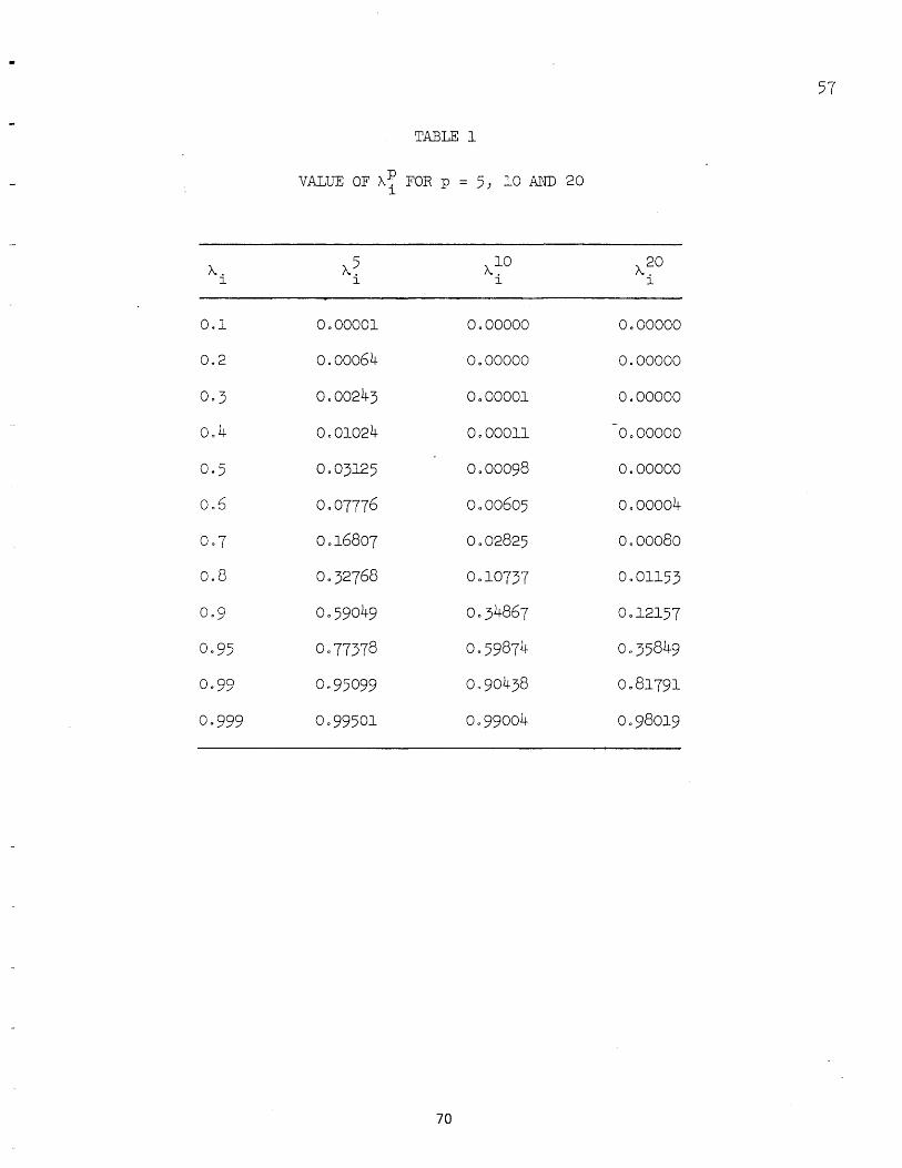
57

TABLE 1

VALUE OF A~ FOR P = 5) 10 AND 20

"A.. "A.~ "A.~O "A.~O l l l l

0.1 0000001 0000000 0000000

0.2 0.00064 0000000 0.00000

0·3 0.00243 0000001 0.00000

004 0.01024 0000011 0.00000

0·5 0.03125 0.00098 0.00000

0.6 0.07776 0.00605 0.00004

007 0016807 0002825 0000080

0.8 0032768 0010737 0001153

009 0059049 0.34867 0012157

0·95 0077378 0·59874 0035849

0099 0.95099 0090438 0081791

0·999 0·99501 0099004 0.98019

70

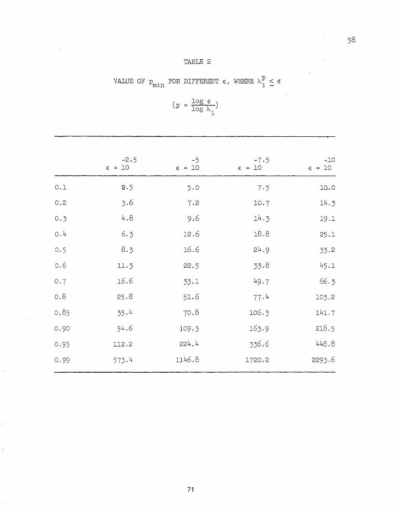
001

0.2

0·3

004

0·5

0.6

0·7

0.8

0.85

0·90

0·95

0·99

TABLE 2

VALUE OF p. FOR DIFFERENT E) WHERE A. ~ < €' IDln l -

-2·5 E = 10

~L5

3·6

4.8

6.3

8.3

11·3

16.6

25.8

35.4

54.6

112.2

573·4

( log E ) P = log /I..

l

-5 E = 10

5·0

7.2

9.6

12.6

16.6

22.5

3301

51.6

70.8

109·3

224.4

1146.8

71

-7·5 E = 10

70)

10·7

1403

1808

2409

3308

4907

77.4

106 0 3

163·9

336.6

1720.2

-10 E = 10

1000

1403

19·1

2501

33,,2

4501

6603

10302

14107

21805

448.8

229306

59

TABLE 3

VALUE OF ~ FOR k = 10

t-.( 1-t... k) 'r ),,( 1_(-.1» ~ - ~ -- (1-t-.·) -.~ 1-1\)

+0.1 0.11111 -0.1 -0.09091

+0.2 0.25000 -0.2 -0.16667

+0·3 0042857 -0·3 -0.23077

+0.4 0.66660 -0.4 -0028568

+0·5 0·99902 -0·5 -0·33301

+0.6 1.49093 -0.6 -0·37273

+0·7 2026742 -0·7 -0040013

+0,8 3057050 -0.8 -0·39672

+0·9 5.86190 -0·9 -0030852

+0·95 7.62400 -0095 -0019549

+0·99 9.46617 -0·99 -0004757

+0·999 9.94516 -00999 -0000498

72

k - ~ max

5

10

15

20

25

50

"­cr

TABLE 4

~lRax " + 2 t-'"max

73

k k + 2

"-cr

0.71429

0.83333

0.88235

0·90909

0092593

0.96154

60

a.

f...i

+0.1

+0.2

+0·3

+0.4 -....J ../:::>

+(L 5

+0.6

+0·7

+0.8

+0·9

TABLE 5

MAXIMUM LOSS, m for k = 5, 10 and 20. (~= k) max

Positive ~ and Positive ~~ b. Positive A and Negative Ai m m

max max

k=5 k=10 k=20 Ai k=5 k==10

-1.643 '-1.949 -2.253 -0.1 -1·748 -2.045

-1.829 -2.276 -2.715 -0.2 -2.134 -2.554

-1·966 -2.580 -3·174 -0·3 -2·592 -3·149

-2.043 -2.880 -3·675 -0.4 , -3·184 -3·911

-2.000 -3·170 -4.248 -0·5 -4.000 -4·954

-1.659 -3·396 -4.918 -0.6 -5,212 ,-6.500.

-1.626 -3·335 -5.676 -0·7 ·-7·222 -9·057

-1.817 -6.213 -0.8 -11.228 -14.148

-1·905 -009 -23~225 -29·384

-0·95 -47 ~202 -59.281

-0·99 -.239· 307 -303·738

k=20

-2·344

-2·980

-3·716-

-4.652

-5·931

-7.821

-10.944

-17.158

-35.745

-72.882 ..

-370·392

CJ\ f-J

TABLE 6a

VAllS OF m FOR POSITIVE f... i AHD POSITIVE t.., (k = 10)

~(l_~lO) ~ ~ = \ 1-~) ; t.. = ~+l (Loss is indicated by a negative value of m. )

log I(~++) "1 - I-ll - 1 m = log ~.

1

""i )..=0·5 ",=0.6 ",=0·7 ~=0.8 ",=0·9 1-..=0·95 ",=0·99 1-..=0·99999· ? •

~=O·99902 1-l=1,49093 1-l=2,,26742 1-l=3·57050 1-l=5.86190 1-l=7.62400 1-l=9.46617 1-'-=9·99999 ... ~·=o.49975 ~=0059854 ~=0.69395 ~=O.78121 ",=0.85427 ~=0"88404 ",=0.90445 ~=0.90909

0.1 -0·903 -1.094 -1.287 -1.493 -10714 -1.830 -1·925 -1·949

-.....J 0.2 -0.68:2 -0·995 -1.297 -1.607 -1.933 -2.103 -2.241 -2.276 U1

0·3 -0.2y3 -00754 -1.210 -1.655 -2.LlO -2.343 -2·532 -2.580

0.4 +0·760 -0,232 -1,044 -1,606 -2.241 -2·,560 -2.816 -2.880

0·5 +10.000 +10026 -0,342 -1·362 -2,282 -2.728 -3·082 -3·170

0,,6 +2,147 +10.000 +1,312 -0.631 -2.090 -2.754 -3·269 -3·396

007 +1.567 +2.856 +100000 +10779 -1.160 -21.295 -3·133 '-3·335

0.8 +1.28B +2,090 +3·749 +10.000 +30427 +0.442 -10399 -1.817 .

0.85 +1.193 +1.879 +}::145 f-6.119 +200725 +6.541 +2,460 +1.651

0·90 +1.117 +10719 +2·755 +4·796 +10e'000 +170824 +28.097 +20:853

0095 +1.053 +1,593 +20477 +4;057 +7 .. 191 +10,000 +13. 442 +14,565

0,99 +1.011 +10514 +2·310 +3.661 +6.080 +7,9<14 +10 .. 000 +10c608 CJ\ I\)

TABLE 6b

VALUE OF m FOR NEGATIVE A.. AND NEGATIVE (.... (k = 10) l

A.(1_A.10 ) 11 11 = ~ 1-/\) j A. = 11+1 (Loss is indicated by a negative value of rn.)

log I (f-L-f1 ) A.. - f-LI l - 1 m == log ( -A.. )

/\. l

l A.=-004 /\=-0·5 A.=-0.6 A.=-007 "-=-008 "-=-009 "-=-0·95 f-L=-0028568 11=-0,33301 f-L=-0037273 11=-0040013 f-L=-0·39672 f-L=-0030852 f-L=-00195 49

~=~03993 ~=-0.49927 ~=-Oo59421 ~=-Oo66703 ~=-0(65761 ~=-0,44617 ~=-0.24299

-0.1 -0·331 -0,425 -00491 -0·532 -0.527 -0·378 -0.060

~ -0.2 +0.209 +0.001 -00132 -0.209 -0.200 +0.100 +1.090

-0·3 +1.193 +0.676 +Oc 404 +0,255 +0.274 +0,904 +1.560

-004 +10.000 +1.96:;· +1.'298 +0·999 +1 0 03~T -+;2·759 +1.258

-0·5 +2,,806 +10.000 +3·081 +20319 +20395 +3· 748 +1.274

-0.6 +2.809 +4.286 +100000 +5.291 +5·577 +3·387 +1.442

-0·7 +3·318 +4.638 +6.605 +10.000 +90278 I +3·878 +1.805

-0.8 +40613 +6.200 +80175 +10·332 +10.000 +5·309 +20597

-009 +8·770 +11.523 +140672 +17.677 +17,2.47 +100000 +5·051

-0,95 +17·209 +22. 0473 +280234 +33·569 +32,820 +19,553 +100000

-0099 +850055 +110,248 +137,780 +162.482 +159,050 +960420 +49·722 G\

\_; ~

64

TABLE 7

COMPARISON OF MODIFIED JUMP SCHEME WITH S.O"Ro METHOD, (k = 9) ell 105(5)

CASE A:

Number of cycles) v

10

20

30

40

50

60

70

80

90

100

110

120

130

140

150

160

170

180

190

200

Problem: Plate on elastic foundationj all edges simply supported (20

4x 20 grid); uniformly

distributed load; aL IN ~ 500,00

Initial vector x(O) = 0

Jump after v = 2,0; at every 10 cycles No Jump

Maximum Residual

r. l

(v)

+0000000675474

+.000000560029

+0000000523234

+.000000480664

+0000000460193

+.000000445069

+0000000428821

+0000000416629

+,000000401553

+-000000386639

+.000000372802

+.000000358177

+-000000343416

+.000000329715

+.000000317545

+,000000305792

+,000000294214

+.000000282871

+0000000271826

+0000000261116

(v+10) 10 r i

A. =- .(v) r.

l

+.82909

+093430

+091864

+095742

+096714

+096350

+097157

+,,96382

+096286

+096422

+n96078

+095879

+096011

+096309

+096300

+096214

+096145

+·96096

+096061

77

Maximum Residual

r. l

(v)

+0000000675474

+,000000560029

+0000000524673

+0000000497577

+,000000483882

+0000000468122

+0000000461347

+0000000453696

+,,000000444594

+0000000439171

+0000000431810

+0000000424427

+0000000417802

+,000000u12259

+ ., 000000405633

+0000000398251

+0000000390364

+0000000383.348

+0000000376902

+0000000370113

A,10 r.

l

(v+10)

r. l

(v)

+,82909

+093687

+094836

+.97248

+09674,3

+·98553

+098342

+097994

+,98781

+'098324

+098291

+098440

+.98674

+098393

+098181

+098020

+098203

+098319

+098199

TABLE 7 (Continued)

COMPARISON OF MODIFIED JUMP SCHEME WITH SeOoRo METHOD 0 (k = 9, w-= 10575)

Problem: Plate on elastic foundation; all edges simply supported (20

4x 20 grid); uniformly

distributed loadj aL IN = 500000

CASE B: Initial vector x(O) interpolated from results from 10 x 10 grid,

Number of cycles, v

10

20

30

40

50

60

70

80

90

100

110

120

130

140

150

160

170

180

190

200

Jump after v = 2:0, a.t ev'ery 10 cycles

Maximum Residual

r. 1

(v)

+0000000349257

-0000000056967

+0000000024089

+0000000015549

+0000000009901

+0000000007687

+0000000006185

+,000000005210

+.000000004486

+.000000003947

.... 000000003560

+,000000003294

-.-.000000003069

~,ooooooo02889

... ,000000002721

+ 000000002576

.... ()Oooooo02450

+.000000002319

+.000000002214

+"000000002101

(v+10) 10 r i

A. = --..-( -v )..----r.

1

- 016312

-042289

+,,64555

+063687

+077659

+080478

+084265

+,,86138

+,88037

+090230

+092591

+093208

+094191

+,,94270

+,·94719

+"95198

+094729

+095529

+094988

78

No Jump

Maximum Residual

r. 1

(v)

+0000000349257

-0000000056967

+ ., 000000026748

+ ,.000000019218

+0000000014659

+0000000C1:l658

+u000000009932

+0000000008567

+,,000000007523

+0000000006803

+ <,000000006139

+,,000000005557

+0000000005128

+ ,.000000004762

+,000000004h38

+0000000004164

+0000000003920

+,000000003705

+0000000003523

+0000000003385

(v+l0) t-. 10 = _r_i ~~_

(v) r.

1

-0016312

-ou46952

+0071848

+0076277

+0079528

+0,85195

+0,86257

+00878.14

+0090429

+0090240

+0··90520

+0,92280

+0,·92863

+0093196

+0093826

+0,.94140

+0094515

+0,·95088

+Ou96083

TABLE 8

EFFECT OF ELIMINATING RESIDUAL COMPONENTS CORRESPONDING -

TO ~. - ( W -1) IN S. 0 0 R. METHOD l

Note: The cycle of jump was executed using 1 + ~ = l/Wo

Maximum Residual r. (v)

Number of l

S.O.R. with SoOoR. with one cycle Over-relaxation

factor) W cycles) v no jump of jump at v=O

10625 10 -0000005465374 +.000002872446

20 -0000000935717 -0000000899836

10900 10 -0000002358422 +.000001319046

20 +rOOOOO1806640 -0000000846318

10 -0000003650364 -.000001964721

20 +0000002929562 -0000001546476

79

66

400~------~------~------~------~----~~

300r-------~--------r--------+--------+-----rH~

0-.. en w ..J U >-U

u.. 200 0

a:: w a:l ~ :J Z

100r-------~--------~-------+------

O~~§§~====±====-~----~----~ o 2 4 6 8 10

III A.I II

I

FIG. I VALUES OF p SUCH .THAT lilA' III = E . I

80

..

10

-

8

'6

2 -..< ..< I I -- -,<

II 4 ---r --::l.

... POSI?

~ /

------------.-- NEGATIVE A ~

2

o

o 0.2 0.4 0.6 0.8 1.0

FIG. 2 VALUES OF p. FOR k = 10

81

o 0.2 o ~f::::::--

0.4 0.6 0.8 1.0

NEGATIVE Ai

20 ---i I -

E

--~------~-.. en w ...J 30 <..)

>-I

u u.. :

0 a::: w CD 40 , ~ :::> z I

50 1--------+--.---.-.-.--- .-.------.-t-----t-----+----l

60~-----~----~---·-+-------r-----+~

FIG. :3 MAGNITUDE OF LOSS m, FOR JL = k = 10

82

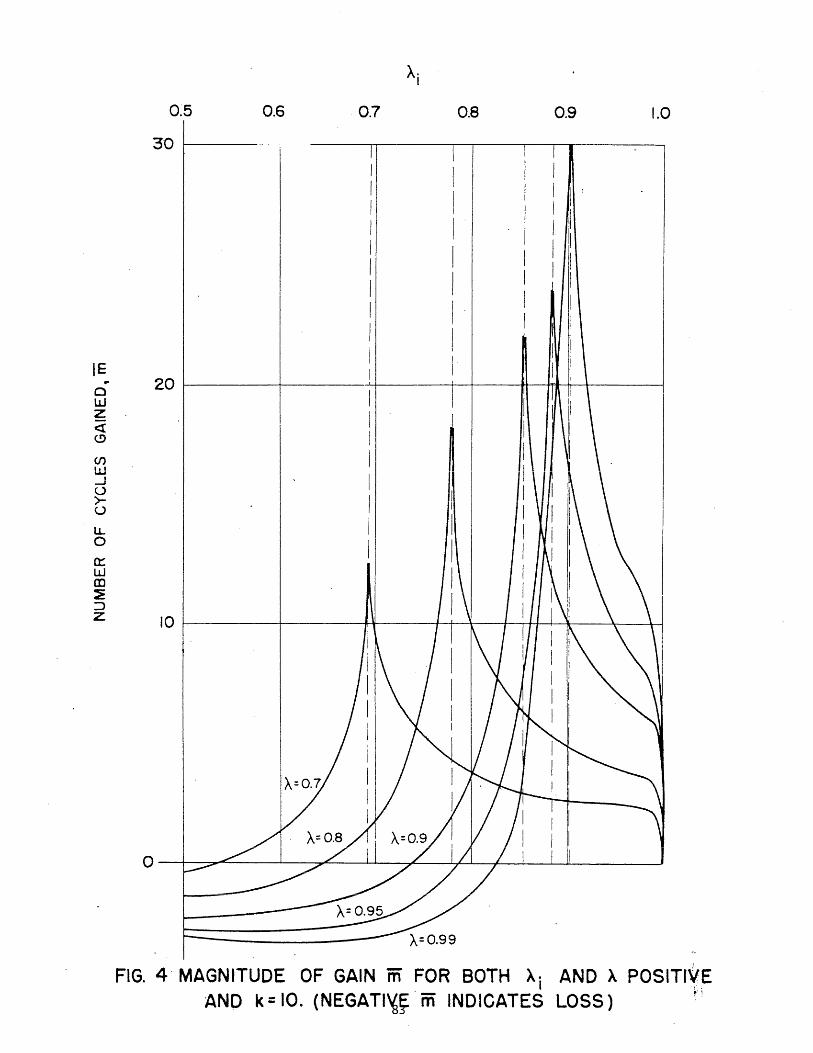
A· I

0~5 0.6 0.7 0.8 0.9 1.0

30

I I :

I

I I !

I I I I

I I I

I I IE I

~ 20 0 w Z <l: <!)

C/) W ..J 0 >-u u. 0

a::: w CD ~ :::> z 10

r ~ ~//

F 5~ - )"=0.99

FIG. 4- MAGNITUDE OF GAIN iii FOR BOTH Ai AND A POSITr¥~ AND k = 10. (NEGATI"~' ffi INDICATES LOSS) ~)

IE r

0 w Z c::t: <.!)

(f) w -1 U >-u LL 0

0:: w en ~ ::> z

30 I I I : I I I I I I I I I I I I I I I I

: I I I 1 I I I I I I I I I I I I I I

20 I I I I I I I I I I I I I I !

! ArO.8

I 10

o ~~----~------~----~--~------~--------~------~ -0.4 -0.5 -0.6 -0.7

A. I

-0.8 -0.9

FIG. 5 MAGNITUDE OF GAIN m FOR BOTH Ai AND A POSITIVE

AND k = 10. (NEGAIJVE m INDICATES LOSS)

-1.0