for the Multiwire Real-Time Back-Reflection Laue ...prism.mit.edu/xray/oldsite/Laue SOP.pdf · Multiwire Real-Time Back-Reflection Laue Diffractometer ... The gas cylinder is attached

$Page 1: for the Multiwire Real-Time Back-Reflection Laue ...prism.mit.edu/xray/oldsite/Laue SOP.pdf · Multiwire Real-Time Back-Reflection Laue Diffractometer ... The gas cylinder is attached$
Page 1 of 20

Revision Date: 27 Feb 2012

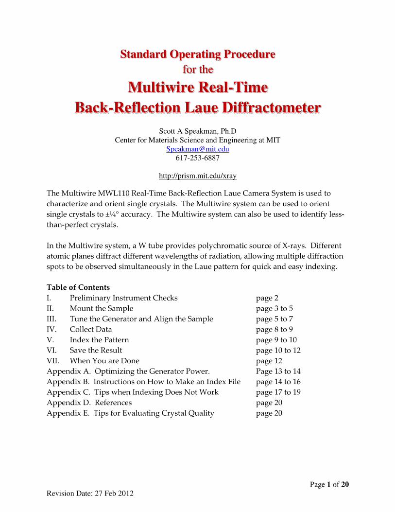
Standard Operating Procedure

for the

Multiwire Real-Time

Back-Reflection Laue Diffractometer

Scott A Speakman, Ph.D

Center for Materials Science and Engineering at MIT

[email protected]

617-253-6887

http://prism.mit.edu/xray

The Multiwire MWL110 Real-Time Back-Reflection Laue Camera System is used to

characterize and orient single crystals. The Multiwire system can be used to orient

single crystals to ±¼° accuracy. The Multiwire system can also be used to identify less-

than-perfect crystals.

In the Multiwire system, a W tube provides polychromatic source of X-rays. Different

atomic planes diffract different wavelengths of radiation, allowing multiple diffraction

spots to be observed simultaneously in the Laue pattern for quick and easy indexing.

Table of Contents

I. Preliminary Instrument Checks page 2

II. Mount the Sample page 3 to 5

III. Tune the Generator and Align the Sample page 5 to 7

IV. Collect Data page 8 to 9

V. Index the Pattern page 9 to 10

VI. Save the Result page 10 to 12

VII. When You are Done page 12

Appendix A. Optimizing the Generator Power. Page 13 to 14

Appendix B. Instructions on How to Make an Index File page 14 to 16

Appendix C. Tips when Indexing Does Not Work page 17 to 19

Appendix D. References page 20

Appendix E. Tips for Evaluating Crystal Quality page 20

Page 2 of 20


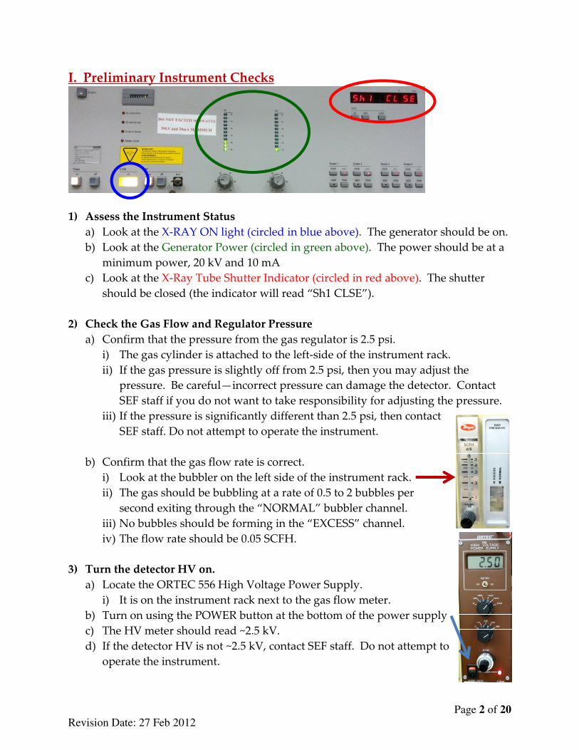
I. Preliminary Instrument Checks

1) Assess the Instrument Status

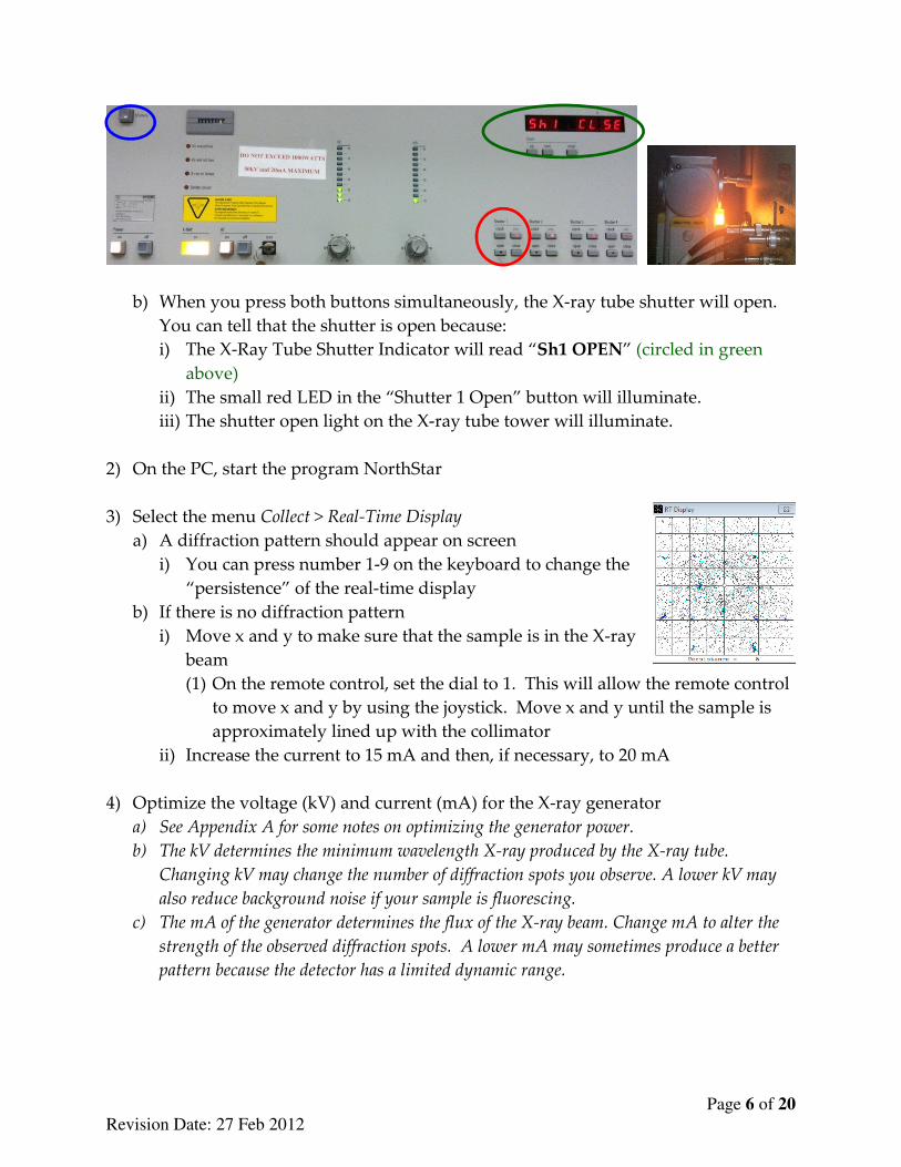
a) Look at the X-RAY ON light (circled in blue above). The generator should be on.

b) Look at the Generator Power (circled in green above). The power should be at a

minimum power, 20 kV and 10 mA

c) Look at the X-Ray Tube Shutter Indicator (circled in red above). The shutter

should be closed (the indicator will read “Sh1 CLSE”).

2) Check the Gas Flow and Regulator Pressure

a) Confirm that the pressure from the gas regulator is 2.5 psi.

i) The gas cylinder is attached to the left-side of the instrument rack.

ii) If the gas pressure is slightly off from 2.5 psi, then you may adjust the

pressure. Be careful—incorrect pressure can damage the detector. Contact

SEF staff if you do not want to take responsibility for adjusting the pressure.

iii) If the pressure is significantly different than 2.5 psi, then contact

SEF staff. Do not attempt to operate the instrument.

b) Confirm that the gas flow rate is correct.

i) Look at the bubbler on the left side of the instrument rack.

ii) The gas should be bubbling at a rate of 0.5 to 2 bubbles per

second exiting through the “NORMAL” bubbler channel.

iii) No bubbles should be forming in the “EXCESS” channel.

iv) The flow rate should be 0.05 SCFH.

3) Turn the detector HV on.

a) Locate the ORTEC 556 High Voltage Power Supply.

i) It is on the instrument rack next to the gas flow meter.

b) Turn on using the POWER button at the bottom of the power supply

c) The HV meter should read ~2.5 kV.

d) If the detector HV is not ~2.5 kV, contact SEF staff. Do not attempt to

operate the instrument.

Page 3 of 20


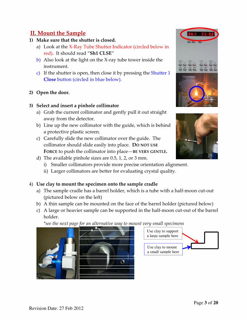
II. Mount the Sample 1) Make sure that the shutter is closed.

a) Look at the X-Ray Tube Shutter Indicator (circled below in

red). It should read “Sh1 CLSE”

b) Also look at the light on the X-ray tube tower inside the

instrument.

c) If the shutter is open, then close it by pressing the Shutter 1

Close button (circled in blue below).

2) Open the door.

3) Select and insert a pinhole collimator

a) Grab the current collimator and gently pull it out straight

away from the detector.

b) Line up the new collimator with the guide, which is behind

a protective plastic screen.

c) Carefully slide the new collimator over the guide. The

collimator should slide easily into place. DO NOT USE

FORCE to push the collimator into place—BE VERY GENTLE.

d) The available pinhole sizes are 0.5, 1, 2, or 3 mm.

i) Smaller collimators provide more precise orientation alignment.

ii) Larger collimators are better for evaluating crystal quality.

4) Use clay to mount the specimen onto the sample cradle

a) The sample cradle has a barrel holder, which is a tube with a half-moon cut-out

(pictured below on the left)

b) A thin sample can be mounted on the face of the barrel holder (pictured below)

c) A large or heavier sample can be supported in the half-moon cut-out of the barrel

holder.

*see the next page for an alternative way to mount very small specimens

Use clay to mount

a small sample here

Use clay to support

a large sample here

Page 4 of 20


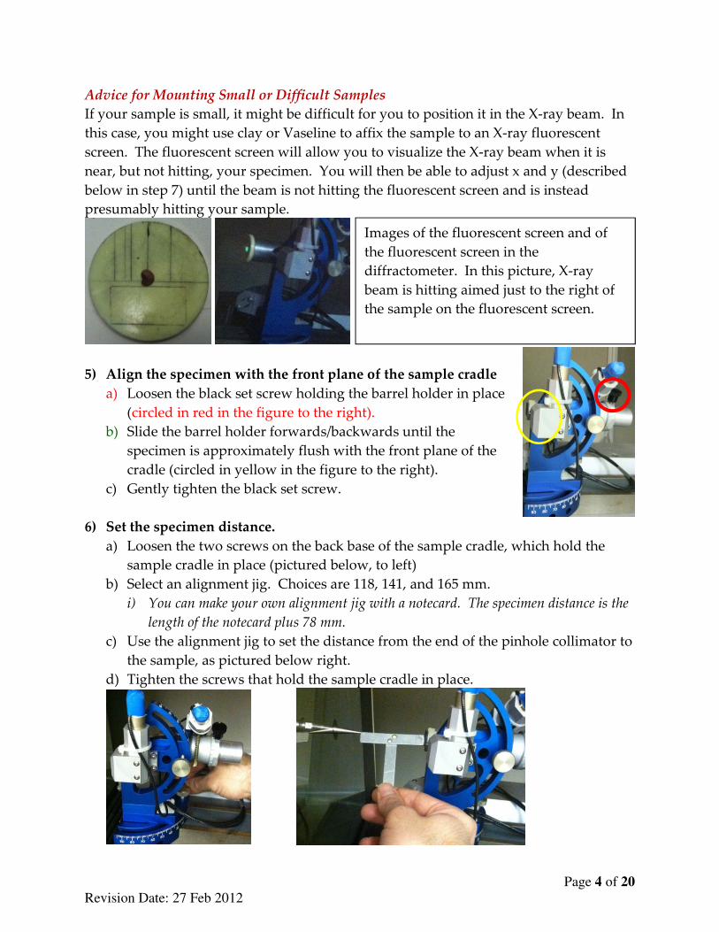
Advice for Mounting Small or Difficult Samples

If your sample is small, it might be difficult for you to position it in the X-ray beam. In

this case, you might use clay or Vaseline to affix the sample to an X-ray fluorescent

screen. The fluorescent screen will allow you to visualize the X-ray beam when it is

near, but not hitting, your specimen. You will then be able to adjust x and y (described

below in step 7) until the beam is not hitting the fluorescent screen and is instead

presumably hitting your sample.

5) Align the specimen with the front plane of the sample cradle

a) Loosen the black set screw holding the barrel holder in place

(circled in red in the figure to the right).

b) Slide the barrel holder forwards/backwards until the

specimen is approximately flush with the front plane of the

cradle (circled in yellow in the figure to the right).

c) Gently tighten the black set screw.

6) Set the specimen distance.

a) Loosen the two screws on the back base of the sample cradle, which hold the

sample cradle in place (pictured below, to left)

b) Select an alignment jig. Choices are 118, 141, and 165 mm.

i) You can make your own alignment jig with a notecard. The specimen distance is the

length of the notecard plus 78 mm.

c) Use the alignment jig to set the distance from the end of the pinhole collimator to

the sample, as pictured below right.

d) Tighten the screws that hold the sample cradle in place.

Images of the fluorescent screen and of

the fluorescent screen in the

diffractometer. In this picture, X-ray

beam is hitting aimed just to the right of

the sample on the fluorescent screen.

Page 5 of 20


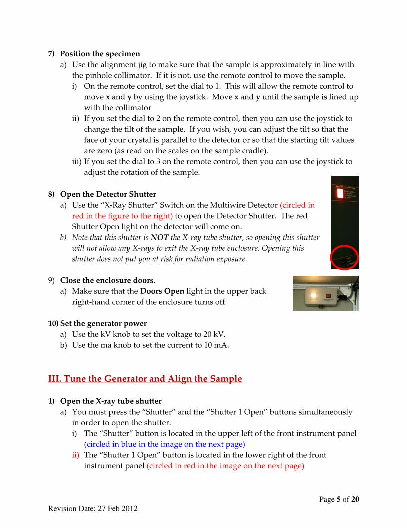
7) Position the specimen

a) Use the alignment jig to make sure that the sample is approximately in line with

the pinhole collimator. If it is not, use the remote control to move the sample.

i) On the remote control, set the dial to 1. This will allow the remote control to

move x and y by using the joystick. Move x and y until the sample is lined up

with the collimator

ii) If you set the dial to 2 on the remote control, then you can use the joystick to

change the tilt of the sample. If you wish, you can adjust the tilt so that the

face of your crystal is parallel to the detector or so that the starting tilt values

are zero (as read on the scales on the sample cradle).

iii) If you set the dial to 3 on the remote control, then you can use the joystick to

adjust the rotation of the sample.

8) Open the Detector Shutter

a) Use the “X-Ray Shutter” Switch on the Multiwire Detector (circled in

red in the figure to the right) to open the Detector Shutter. The red

Shutter Open light on the detector will come on.

b) Note that this shutter is NOT the X-ray tube shutter, so opening this shutter

will not allow any X-rays to exit the X-ray tube enclosure. Opening this

shutter does not put you at risk for radiation exposure.

9) Close the enclosure doors.

a) Make sure that the Doors Open light in the upper back

right-hand corner of the enclosure turns off.

10) Set the generator power

a) Use the kV knob to set the voltage to 20 kV.

b) Use the ma knob to set the current to 10 mA.

III. Tune the Generator and Align the Sample

1) Open the X-ray tube shutter

a) You must press the “Shutter” and the “Shutter 1 Open” buttons simultaneously

in order to open the shutter.

i) The “Shutter” button is located in the upper left of the front instrument panel

(circled in blue in the image on the next page)

ii) The “Shutter 1 Open” button is located in the lower right of the front

instrument panel (circled in red in the image on the next page)

Page 6 of 20


b) When you press both buttons simultaneously, the X-ray tube shutter will open.

You can tell that the shutter is open because:

i) The X-Ray Tube Shutter Indicator will read “Sh1 OPEN” (circled in green

above)

ii) The small red LED in the “Shutter 1 Open” button will illuminate.

iii) The shutter open light on the X-ray tube tower will illuminate.

2) On the PC, start the program NorthStar

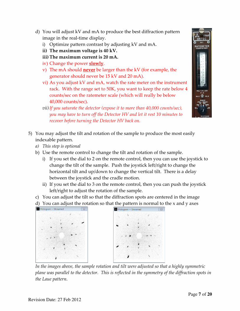
3) Select the menu Collect > Real-Time Display

a) A diffraction pattern should appear on screen

i) You can press number 1-9 on the keyboard to change the

“persistence” of the real-time display

b) If there is no diffraction pattern

i) Move x and y to make sure that the sample is in the X-ray

beam

(1) On the remote control, set the dial to 1. This will allow the remote control

to move x and y by using the joystick. Move x and y until the sample is

approximately lined up with the collimator

ii) Increase the current to 15 mA and then, if necessary, to 20 mA

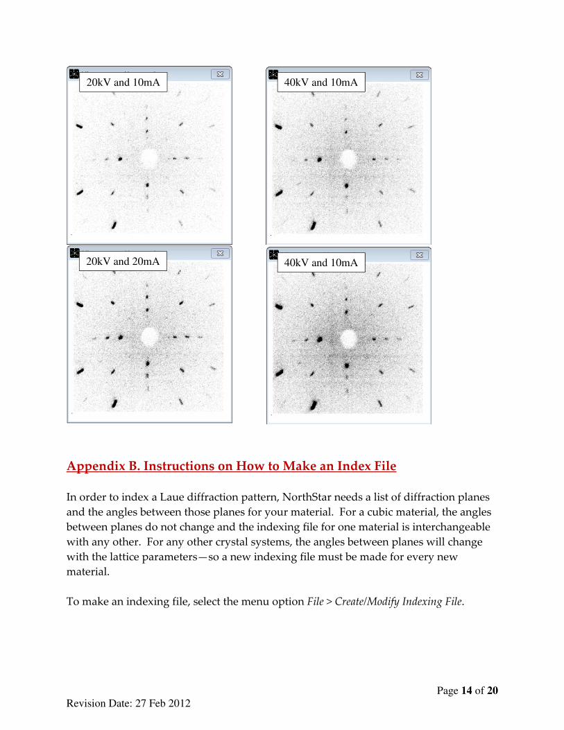
4) Optimize the voltage (kV) and current (mA) for the X-ray generator

a) See Appendix A for some notes on optimizing the generator power.

b) The kV determines the minimum wavelength X-ray produced by the X-ray tube.

Changing kV may change the number of diffraction spots you observe. A lower kV may

also reduce background noise if your sample is fluorescing.

c) The mA of the generator determines the flux of the X-ray beam. Change mA to alter the

strength of the observed diffraction spots. A lower mA may sometimes produce a better

pattern because the detector has a limited dynamic range.

Page 7 of 20


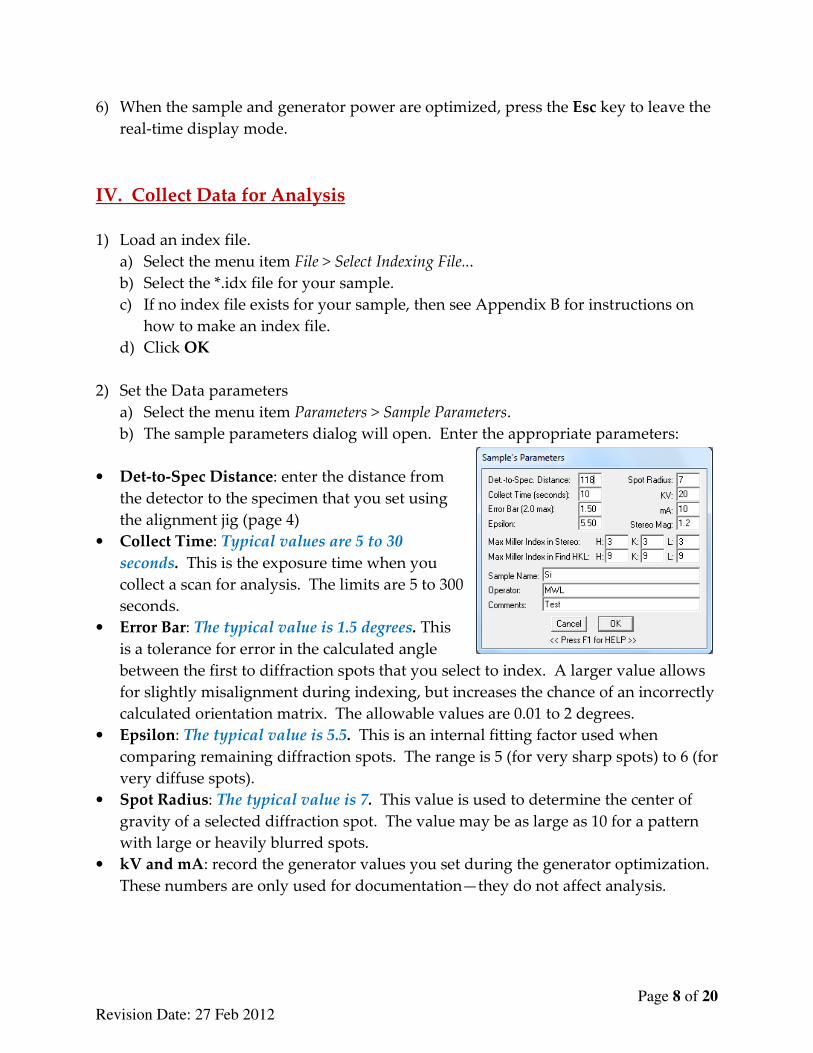
d) You will adjust kV and mA to produce the best diffraction pattern

image in the real-time display.

i) Optimize pattern contrast by adjusting kV and mA.

ii) The maximum voltage is 40 kV.

iii) The maximum current is 20 mA.

iv) Change the power slowly.

v) The mA should never be larger than the kV (for example, the

generator should never be 15 kV and 20 mA).

vi) As you adjust kV and mA, watch the rate meter on the instrument

rack. With the range set to 50K, you want to keep the rate below 4

counts/sec on the ratemeter scale (which will really be below

40,000 counts/sec).

vii) If you saturate the detector (expose it to more than 40,000 counts/sec),

you may have to turn off the Detector HV and let it rest 10 minutes to

recover before turning the Detector HV back on.

5) You may adjust the tilt and rotation of the sample to produce the most easily

indexable pattern.

a) This step is optional

b) Use the remote control to change the tilt and rotation of the sample.

i) If you set the dial to 2 on the remote control, then you can use the joystick to

change the tilt of the sample. Push the joystick left/right to change the

horizontal tilt and up/down to change the vertical tilt. There is a delay

between the joystick and the cradle motion.

ii) If you set the dial to 3 on the remote control, then you can push the joystick

left/right to adjust the rotation of the sample.

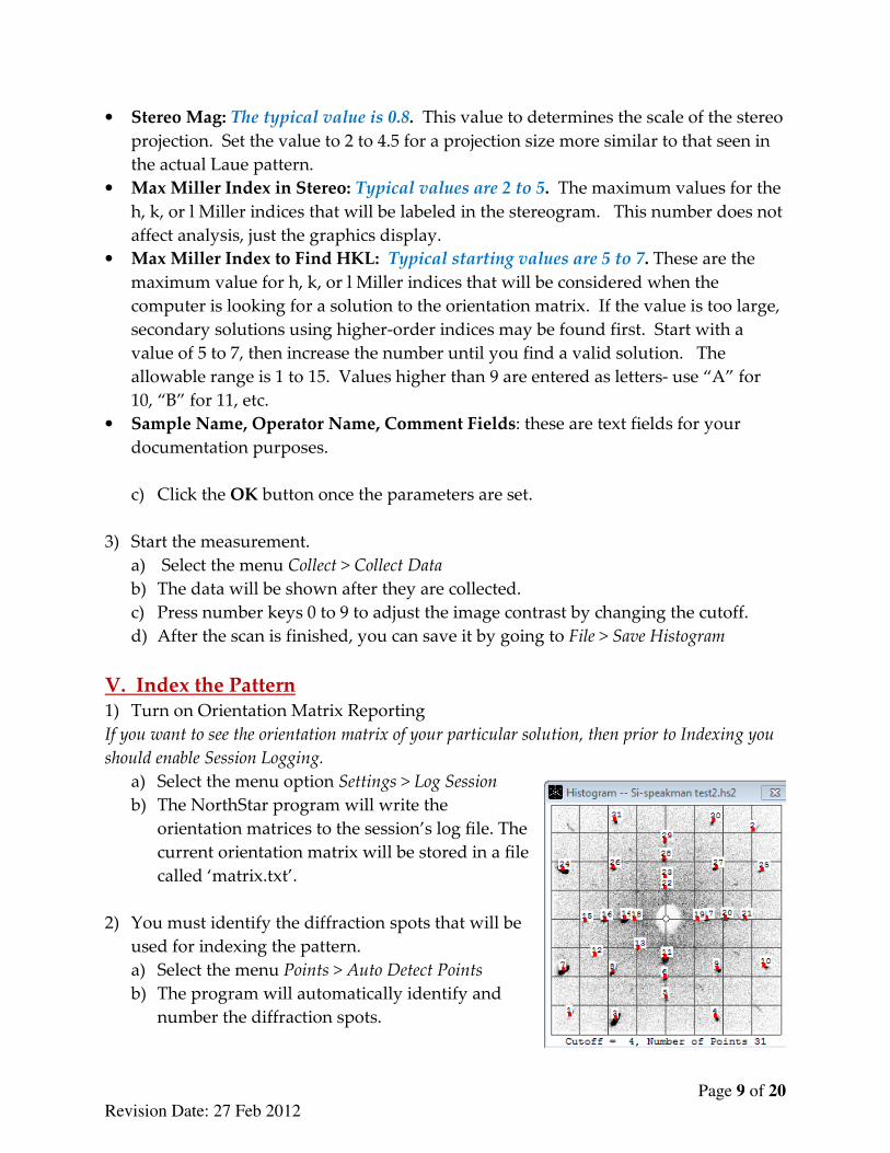
c) You can adjust the tilt so that the diffraction spots are centered in the image

d) You can adjust the rotation so that the pattern is normal to the x and y axes

In the images above, the sample rotation and tilt were adjusted so that a highly symmetric

plane was parallel to the detector. This is reflected in the symmetry of the diffraction spots in

the Laue pattern.

Page 8 of 20


6) When the sample and generator power are optimized, press the Esc key to leave the

real-time display mode.

IV. Collect Data for Analysis

1) Load an index file.

a) Select the menu item File > Select Indexing File...

b) Select the *.idx file for your sample.

c) If no index file exists for your sample, then see Appendix B for instructions on

how to make an index file.

d) Click OK

2) Set the Data parameters

a) Select the menu item Parameters > Sample Parameters.

b) The sample parameters dialog will open. Enter the appropriate parameters:

• Det-to-Spec Distance: enter the distance from

the detector to the specimen that you set using

the alignment jig (page 4)

• Collect Time: Typical values are 5 to 30

seconds. This is the exposure time when you

collect a scan for analysis. The limits are 5 to 300

seconds.

• Error Bar: The typical value is 1.5 degrees. This

is a tolerance for error in the calculated angle

between the first to diffraction spots that you select to index. A larger value allows

for slightly misalignment during indexing, but increases the chance of an incorrectly

calculated orientation matrix. The allowable values are 0.01 to 2 degrees.

• Epsilon: The typical value is 5.5. This is an internal fitting factor used when

comparing remaining diffraction spots. The range is 5 (for very sharp spots) to 6 (for

very diffuse spots).

• Spot Radius: The typical value is 7. This value is used to determine the center of

gravity of a selected diffraction spot. The value may be as large as 10 for a pattern

with large or heavily blurred spots.

• kV and mA: record the generator values you set during the generator optimization.

These numbers are only used for documentation—they do not affect analysis.

Page 9 of 20


• Stereo Mag: The typical value is 0.8. This value to determines the scale of the stereo

projection. Set the value to 2 to 4.5 for a projection size more similar to that seen in

the actual Laue pattern.

• Max Miller Index in Stereo: Typical values are 2 to 5. The maximum values for the

h, k, or l Miller indices that will be labeled in the stereogram. This number does not

affect analysis, just the graphics display.

• Max Miller Index to Find HKL: Typical starting values are 5 to 7. These are the

maximum value for h, k, or l Miller indices that will be considered when the

computer is looking for a solution to the orientation matrix. If the value is too large,

secondary solutions using higher-order indices may be found first. Start with a

value of 5 to 7, then increase the number until you find a valid solution. The

allowable range is 1 to 15. Values higher than 9 are entered as letters- use “A” for

10, “B” for 11, etc.

• Sample Name, Operator Name, Comment Fields: these are text fields for your

documentation purposes.

c) Click the OK button once the parameters are set.

3) Start the measurement.

a) Select the menu Collect > Collect Data

b) The data will be shown after they are collected.

c) Press number keys 0 to 9 to adjust the image contrast by changing the cutoff.

d) After the scan is finished, you can save it by going to File > Save Histogram

V. Index the Pattern 1) Turn on Orientation Matrix Reporting

If you want to see the orientation matrix of your particular solution, then prior to Indexing you

should enable Session Logging.

a) Select the menu option Settings > Log Session

b) The NorthStar program will write the

orientation matrices to the session’s log file. The

current orientation matrix will be stored in a file

called ‘matrix.txt’.

2) You must identify the diffraction spots that will be

used for indexing the pattern.

a) Select the menu Points > Auto Detect Points

b) The program will automatically identify and

number the diffraction spots.

Page 10 of 20


c) If the program does not automatically detect all of the observed diffraction spots,

you may manually add data points

i) Select the menu Points > Add Points

ii) The mouse cursor will become a crosshair.

iii) Move the crosshair over each data point that you wish to add and left-click.

iv) When you have added all data points that you want to use for indexing, press

the Esc key.

d) You can erase diffraction spots if they are weak or misshapen and might

compromise your indexing result

i) Select the menu Points > Delete Points

ii) Left-click on each diffraction spot you want to remove

e) When you are done, press the Esc key.

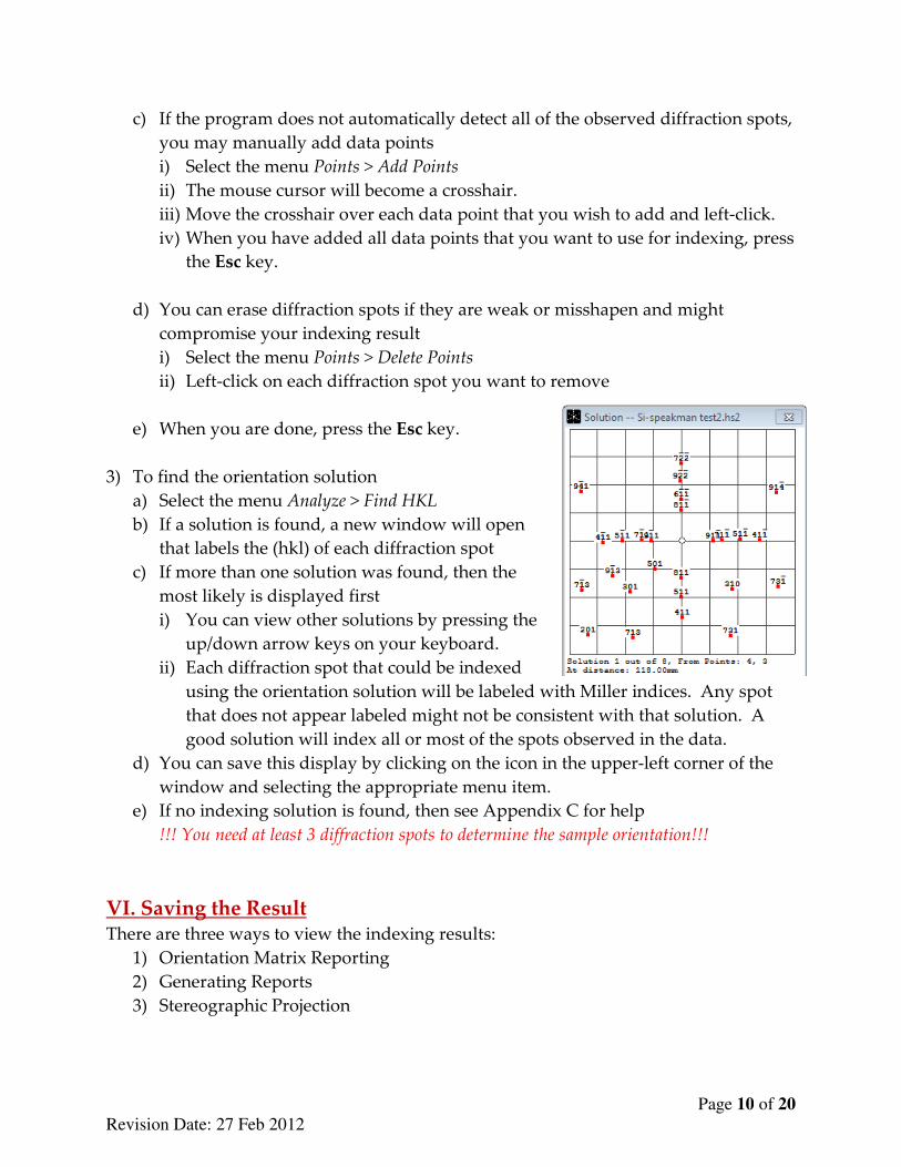
3) To find the orientation solution

a) Select the menu Analyze > Find HKL

b) If a solution is found, a new window will open

that labels the (hkl) of each diffraction spot

c) If more than one solution was found, then the

most likely is displayed first

i) You can view other solutions by pressing the

up/down arrow keys on your keyboard.

ii) Each diffraction spot that could be indexed

using the orientation solution will be labeled with Miller indices. Any spot

that does not appear labeled might not be consistent with that solution. A

good solution will index all or most of the spots observed in the data.

d) You can save this display by clicking on the icon in the upper-left corner of the

window and selecting the appropriate menu item.

e) If no indexing solution is found, then see Appendix C for help

!!! You need at least 3 diffraction spots to determine the sample orientation!!!

VI. Saving the Result There are three ways to view the indexing results:

1) Orientation Matrix Reporting

2) Generating Reports

3) Stereographic Projection

Page 11 of 20


The orientation matrix reporting was turned on as described in page 9 above.

1) Generating Reports

The Data Report and Test Output Menu-items in the Analyze menu will provide

additional information about your indexing solution. To generate a report,

a) Select Analyze > Data Report or Analyze > Test Output

b) From the report, you can select to save or print.

a. If you save, you will save with only the text output

b. If you print, you can choose whether or not to include the image of the

Laue pattern (ie histogram). To create an electronic file, change the printer

to Cute PDF to create a PDF file with the report and Laue pattern when

you select to print.

i. Select File > Printer Setup to change the printer.

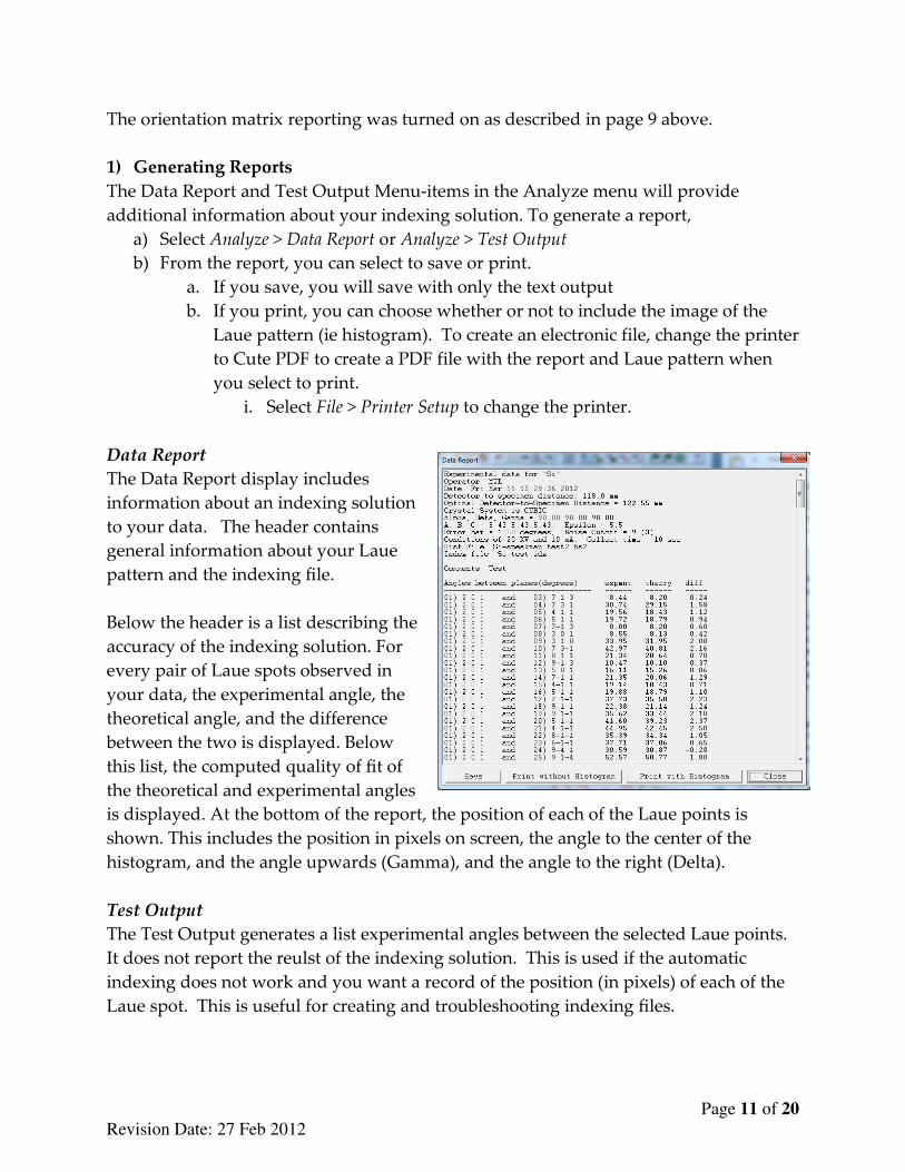
Data Report

The Data Report display includes

information about an indexing solution

to your data. The header contains

general information about your Laue

pattern and the indexing file.

Below the header is a list describing the

accuracy of the indexing solution. For

every pair of Laue spots observed in

your data, the experimental angle, the

theoretical angle, and the difference

between the two is displayed. Below

this list, the computed quality of fit of

the theoretical and experimental angles

is displayed. At the bottom of the report, the position of each of the Laue points is

shown. This includes the position in pixels on screen, the angle to the center of the

histogram, and the angle upwards (Gamma), and the angle to the right (Delta).

Test Output

The Test Output generates a list experimental angles between the selected Laue points.

It does not report the reulst of the indexing solution. This is used if the automatic

indexing does not work and you want a record of the position (in pixels) of each of the

Laue spot. This is useful for creating and troubleshooting indexing files.

Page 12 of 20


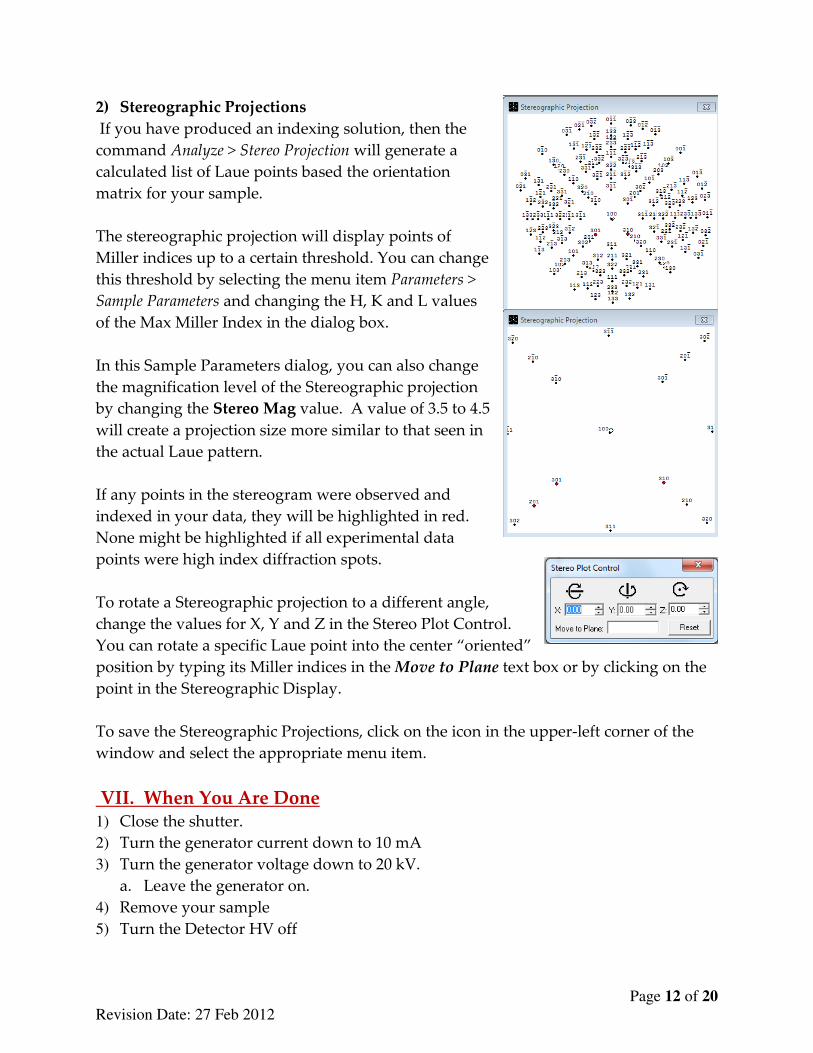
2) Stereographic Projections

If you have produced an indexing solution, then the

command Analyze > Stereo Projection will generate a

calculated list of Laue points based the orientation

matrix for your sample.

The stereographic projection will display points of

Miller indices up to a certain threshold. You can change

this threshold by selecting the menu item Parameters >

Sample Parameters and changing the H, K and L values

of the Max Miller Index in the dialog box.

In this Sample Parameters dialog, you can also change

the magnification level of the Stereographic projection

by changing the Stereo Mag value. A value of 3.5 to 4.5

will create a projection size more similar to that seen in

the actual Laue pattern.

If any points in the stereogram were observed and

indexed in your data, they will be highlighted in red.

None might be highlighted if all experimental data

points were high index diffraction spots.

To rotate a Stereographic projection to a different angle,

change the values for X, Y and Z in the Stereo Plot Control.

You can rotate a specific Laue point into the center “oriented”

position by typing its Miller indices in the Move to Plane text box or by clicking on the

point in the Stereographic Display.

To save the Stereographic Projections, click on the icon in the upper-left corner of the

window and select the appropriate menu item.

VII. When You Are Done 1) Close the shutter.

2) Turn the generator current down to 10 mA

3) Turn the generator voltage down to 20 kV.

a. Leave the generator on.

4) Remove your sample

5) Turn the Detector HV off

Page 13 of 20


Appendix A. Optimizing the Generator Power. The tungsten X-ray tube in Laue diffractometer will produce a continuum of X-

radiation with few characteristic X-rays.

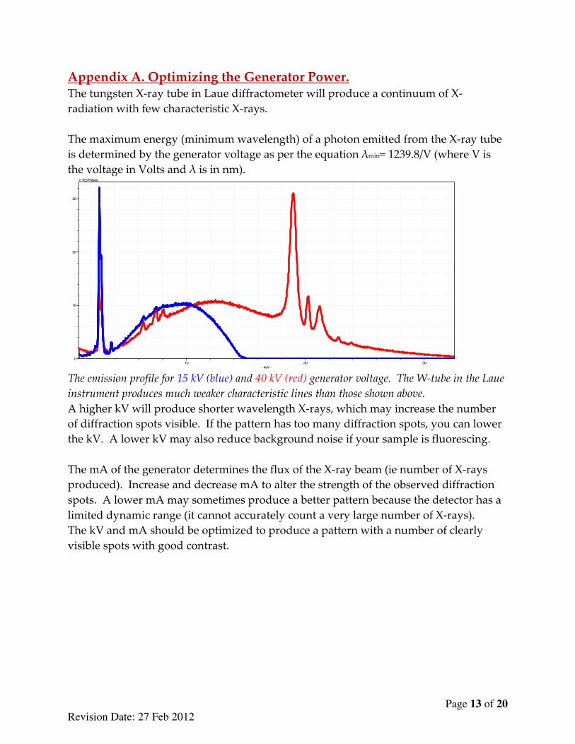
The maximum energy (minimum wavelength) of a photon emitted from the X-ray tube

is determined by the generator voltage as per the equation λmin= 1239.8/V (where V is

the voltage in Volts and λ is in nm).

The emission profile for 15 kV (blue) and 40 kV (red) generator voltage. The W-tube in the Laue

instrument produces much weaker characteristic lines than those shown above.

A higher kV will produce shorter wavelength X-rays, which may increase the number

of diffraction spots visible. If the pattern has too many diffraction spots, you can lower

the kV. A lower kV may also reduce background noise if your sample is fluorescing.

The mA of the generator determines the flux of the X-ray beam (ie number of X-rays

produced). Increase and decrease mA to alter the strength of the observed diffraction

spots. A lower mA may sometimes produce a better pattern because the detector has a

limited dynamic range (it cannot accurately count a very large number of X-rays).

The kV and mA should be optimized to produce a pattern with a number of clearly

visible spots with good contrast.

10 20 30

- keV -

0

10

20

30

x 1E3 Pulses

Page 14 of 20


Appendix B. Instructions on How to Make an Index File

In order to index a Laue diffraction pattern, NorthStar needs a list of diffraction planes

and the angles between those planes for your material. For a cubic material, the angles

between planes do not change and the indexing file for one material is interchangeable

with any other. For any other crystal systems, the angles between planes will change

with the lattice parameters—so a new indexing file must be made for every new

material.

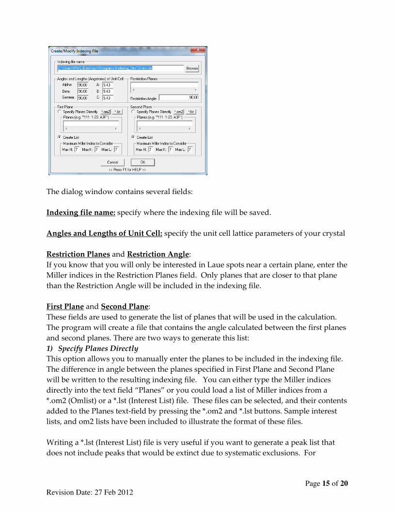
To make an indexing file, select the menu option File > Create/Modify Indexing File.

20kV and 10mA 40kV and 10mA

20kV and 20mA 40kV and 10mA

Page 15 of 20


The dialog window contains several fields:

Indexing file name: specify where the indexing file will be saved.

Angles and Lengths of Unit Cell: specify the unit cell lattice parameters of your crystal

Restriction Planes and Restriction Angle:

If you know that you will only be interested in Laue spots near a certain plane, enter the

Miller indices in the Restriction Planes field. Only planes that are closer to that plane

than the Restriction Angle will be included in the indexing file.

First Plane and Second Plane:

These fields are used to generate the list of planes that will be used in the calculation.

The program will create a file that contains the angle calculated between the first planes

and second planes. There are two ways to generate this list:

1) Specify Planes Directly

This option allows you to manually enter the planes to be included in the indexing file.

The difference in angle between the planes specified in First Plane and Second Plane

will be written to the resulting indexing file. You can either type the Miller indices

directly into the text field “Planes” or you could load a list of Miller indices from a

*.om2 (Omlist) or a *.lst (Interest List) file. These files can be selected, and their contents

added to the Planes text-field by pressing the *.om2 and *.lst buttons. Sample interest

lists, and om2 lists have been included to illustrate the format of these files.

Writing a *.lst (Interest List) file is very useful if you want to generate a peak list that

does not include peaks that would be extinct due to systematic exclusions. For

Page 16 of 20


example, using the Create List option below would generate a list with every possible

(hkl), while you might know that because of symmetry elements in your crystal

structure there are many peaks that would be systematically absent. You could look up

a PDF reference card for your material and use that to create a list only of peaks that

will actually diffract for your material.

2) Create List

This option will create a list of all Miller indices with H, K and L values less than Max

H, Max K and Max L respectively. Note that large values for Max H, Max K and Max L

will create very large amounts of output.

Once the index file has been generated, it is ready for use. However, if a warning

message appeared noting that too many angles were generated, try regenerating the

indexing file using fewer planes.

Once you click OK, the indexing file, with extension *.idx, will be created. You can

view and manually edit this indexing file by opening the file in Windows Notepad (do

not use a word processor).

The indexing file format

An indexing file consists of three main sections; the header, the angles, and the tail.

These are described as follows:

1. The header contains information about the crystal system from which the angles

were generated. These include:

1. LINE 1: a, b, and c parameters (in Angstroms).

2. LINE 2: alpha, beta, gamma (in degrees).

Behind the hash-marks (#), there may appear properties that allow NorthStar to infer

how the indexing file was originally created.

2. The angle section contains the angles between pairs of Miller indices. Each entry is

one line consisting of the following components:

Angle*100 Miller indices #1 Miller indices #2

3. The tail section contains a terminating angle of 0000 followed by one or more

comment lines.

Page 17 of 20


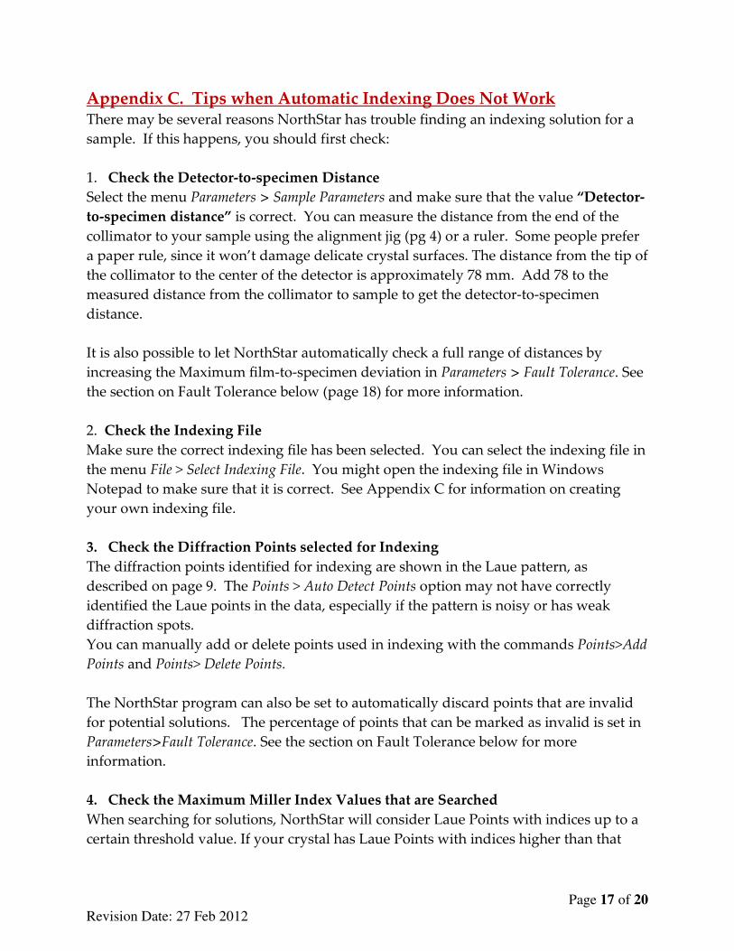
Appendix C. Tips when Automatic Indexing Does Not Work There may be several reasons NorthStar has trouble finding an indexing solution for a

sample. If this happens, you should first check:

1. Check the Detector-to-specimen Distance

Select the menu Parameters > Sample Parameters and make sure that the value “Detector-

to-specimen distance” is correct. You can measure the distance from the end of the

collimator to your sample using the alignment jig (pg 4) or a ruler. Some people prefer

a paper rule, since it won’t damage delicate crystal surfaces. The distance from the tip of

the collimator to the center of the detector is approximately 78 mm. Add 78 to the

measured distance from the collimator to sample to get the detector-to-specimen

distance.

It is also possible to let NorthStar automatically check a full range of distances by

increasing the Maximum film-to-specimen deviation in Parameters > Fault Tolerance. See

the section on Fault Tolerance below (page 18) for more information.

2. Check the Indexing File

Make sure the correct indexing file has been selected. You can select the indexing file in

the menu File > Select Indexing File. You might open the indexing file in Windows

Notepad to make sure that it is correct. See Appendix C for information on creating

your own indexing file.

3. Check the Diffraction Points selected for Indexing

The diffraction points identified for indexing are shown in the Laue pattern, as

described on page 9. The Points > Auto Detect Points option may not have correctly

identified the Laue points in the data, especially if the pattern is noisy or has weak

diffraction spots.

You can manually add or delete points used in indexing with the commands Points>Add

Points and Points> Delete Points.

The NorthStar program can also be set to automatically discard points that are invalid

for potential solutions. The percentage of points that can be marked as invalid is set in

Parameters>Fault Tolerance. See the section on Fault Tolerance below for more

information.

4. Check the Maximum Miller Index Values that are Searched

When searching for solutions, NorthStar will consider Laue Points with indices up to a

certain threshold value. If your crystal has Laue Points with indices higher than that

Page 18 of 20


threshold, these points will be marked as invalid. To increase this threshold, go to the

menu Parameters>Sample Parameters and change the H, K and L values for the Max

Miller

5. Check the Fitting Parameter Epsilon

In the dialog window for menu Parameters>Sample Parameters you can check the value

for Epsilon. Epsilon, a fitting parameter, should not be less than 5.0 for sharp

diffraction spots and can be made as large as 6.0 for crystals with bigger or more diffuse

spots. A value of 5.5 is appropriate for most situations.

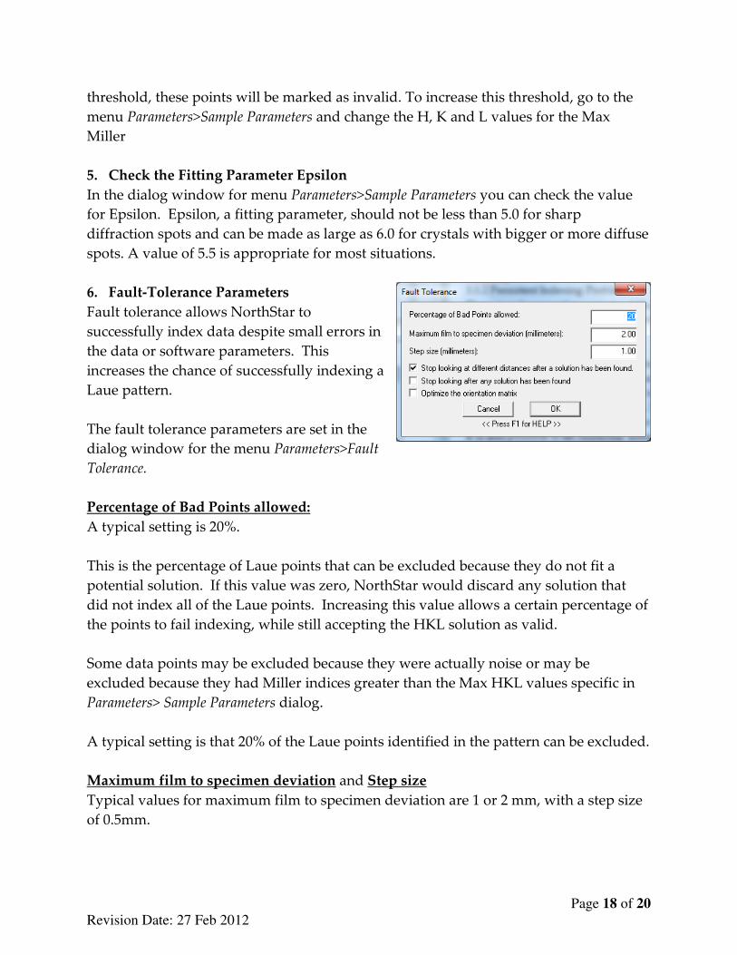
6. Fault-Tolerance Parameters

Fault tolerance allows NorthStar to

successfully index data despite small errors in

the data or software parameters. This

increases the chance of successfully indexing a

Laue pattern.

The fault tolerance parameters are set in the

dialog window for the menu Parameters>Fault

Tolerance.

Percentage of Bad Points allowed:

A typical setting is 20%.

This is the percentage of Laue points that can be excluded because they do not fit a

potential solution. If this value was zero, NorthStar would discard any solution that

did not index all of the Laue points. Increasing this value allows a certain percentage of

the points to fail indexing, while still accepting the HKL solution as valid.

Some data points may be excluded because they were actually noise or may be

excluded because they had Miller indices greater than the Max HKL values specific in

Parameters> Sample Parameters dialog.

A typical setting is that 20% of the Laue points identified in the pattern can be excluded.

Maximum film to specimen deviation and Step size

Typical values for maximum film to specimen deviation are 1 or 2 mm, with a step size

of 0.5mm.

Page 19 of 20


The detector to specimen distance is set in the Parameters>Sample Parameters dialog.

There may be a small error between the value you entered and the actual distance. The

parameter “Maximum film to specimen deviation” allows solutions to deviate from

this detector to specimen distance by a certain amount of millimeters. NorthStar will

test solutions with a range of distances around the specific detector-to-specimen

distance and try to find a solution for each of them. The “Step size” is how large the

steps will be for testing different distances. A smaller step size will allow the software

to test more potential distances between the set value and maximum deviation.

A large value will provide more tolerance for incorrect distances but will greatly

increase the time for the indexing calculation. A value of 1 or 2 mm is a good starting

point. If no solution is found, this could be increased to a maximum deviation of 5mm.

Stop looking at different distances after a solution has been found

This setting is usually checked.

When this setting is turned on, NorthStar will stop searching for new solutions at

different distances after a solution has been found. This option is used so that if

NorthStar finds an indexing solution at the specific detector-to-specimen distance, then

it will not consume time testing solutions at other distances. This option will usually

save time while finding HKL solutions. However, you might turn this often off if the

program keeps stopping after it finds a solution that you judge to be incorrect—and

perhaps a better solution could be found at a different distance.

Stop looking after any solution has been found

This setting is usually unchecked.

When this option is turned on, NorthStar will stop looking for solutions after any

solution has been found. This may save time, but may also cause the program to settle

on a poor solution rather than finding the best solution.

Optimize the orientation matrix

This setting is usually unchecked.

If this option is turned on, then after a solution is found the program will refine the

solution to fit all of the data points as well as possible. Turning this option on will slow

down the search for indexing solutions. However, after the optimization the solution

may contain more Laue spots in the indexing solution because it will be able to improve

the solution to include Laue spots that were originally excluded.

Page 20 of 20


Appendix D. References • EA Wood, Crystal Orientation Manual, Columbia University Press, New York (1963)

• “A Real-Time Back-Reflection Laue Camera ,” DH Bilderback, J. Appl. Cryst. (1979)

12, 95-98.

• “Angle Calculations for 3- and 4-circle X-ray and neutron diffractometers,” WR

Busing and HA Levy, Acta Cryst (1967), 22, pp 457-464.

• “On Refinement of the Crystal Orientation Matrix and Lattice Contants with

Diffractometer Data,” DP Shoemaker and G Bassi, Acta Cryst (1970) A26 pg 97-.

• Cullity, B. D. Elements of Xray Diffraction. 2nd ed. Reading: Addison-Wesley Pub.

Co., 1978.

• Sands, Donald. Introduction to Crystallography. New York:W. A. Benjamin, 1969.

• Barrett C.S. and Massalski T.B., Structure of Metals, 1966.

• Nuffield E.W., X-ray Diffraction Methods, 1966.

• Semat H. and Albright J.R., Introduction to Atomic and Nuclear Physics, 5th edition,

1972.

• Wyckoff R.W.G., Crystal structures, Volume 1, 1963.

Appendix E. Tips for Evaluating Crystal Quality

If you are evaluating crystal quality, then you want to collect data from as large a

fraction of your sample as possible. You are looking for two or more stereograph

projections in the Laue pattern, which would indicate two or more domains.

You should calculate an ideal Laue pattern using the Stereographic Projection in

NorthStar or the program JCrystal.

In JCrystal, you will enter the unit cell lattice parameters on the home screen. Then

select the menu View > Laue Patterns to create the ideal Laue pattern for a single crystal.

In the option for the Laue Pattern, on the righ-hand side of the dialog window, be sure

to set the mode to Back Reflection rather than Transmission. The Film Diameter is

300mm.

Documents

for the Multiwire Real-Time Back-Reflection Laue ...prism.mit.edu/xray/oldsite/Laue SOP.pdf · Multiwire Real-Time Back-Reflection Laue Diffractometer ... The gas cylinder is attached