Embed Size (px)
Citation preview
The Pennsylvania State University
The Graduate School
College of Health and Human Development
FORCE- AND POWER-VELOCITY RELATIONSHIPS
IN A MULTI-JOINT MOVEMENT
A Thesis in
Exercise and Sport Science
by
Andrew Timothy Todd Hardyk
2000 Andrew Timothy Todd Hardyk
Submitted in Partial Fulfillment of the Requirements
for the Degree of
Doctor of Philosophy
December 2000
We approve the thesis of Andrew Timothy Todd Hardyk
Date of Signature _____________________________ _______________ Vladimir M. Zatsiorsky Professor of Kinesiology Thesis Advisor Chair of Committee _____________________________ _______________ Richard C. Nelson Professor Emeritus of Biomechanics _____________________________ _______________ William J. Kraemer Professor of Applied Physiology _____________________________ _______________ H. Joseph Sommer III Professor of Mechanical Engineering _____________________________ _______________ Mark L. Latash Professor of Kinesiology Graduate Program Director, Department of Kinesiology
iii
Abstract
Force-velocity characteristics in multi-joint movements, specifically the vertical
jump, have been relatively unexplored in the literature. There were five main goals in
this study: 1) to accurately define the force-velocity relationships for a multi-joint
movement and compare them to Hill’s classic force-velocity curve, 2) to compare several
options for presenting force-velocity curves in a multi-joint movement, 3) to accurately
define the power-load and power-velocity relationships in a multi-joint movement for the
ranges of force and velocity that were obtainable, 4) since the entire theoretical power-
velocity curve was not obtainable because of physical limitations, to determine whether
the data in this experiment lies in the ascending or descending portion of the theoretical
power-velocity curve, and 5) to determine the load and velocity at which maximum
power was produced.
Ten well-trained subjects were asked to perform maximum effort,
noncountermovement vertical jumps with a range (80% of bodyweight unloading to
125% of bodyweight additional loading) of external loads applied. Each subject
performed 28-34 trials with two trials at each condition. The instant of the maximum
levels of the various velocity measures was used as the time to measure all of the other
variables and the trial with the highest maximum center of mass velocity was selected for
analysis.
Relationships were identified as ‘Hill-like’ if they were descending, had upward
concavity, and 0<a/Fo<1. All of the variables studied in this investigation (maximum
velocity of the center of mass, maximum knee angular velocity, maximum leg extension
velocity, ground reaction force, and knee moment) were plotted against load. None of
these relationships compared well with Hill’s curve. Various logical combinations of
these variables were compared to each other and to Hill’s curve. Only ground reaction
force vs. maximum center of mass velocity (video), vs. maximum knee angular velocity,
and vs. maximum leg extension velocity were Hill-like. The best fit was the ground
reaction force vs. maximum center of mass velocity (video) relationship, mathematically
fit with Hill’s curve.
iv
Power, calculated by multiplying ground reaction force and maximum center of
mass velocity, varied as expected with maximum center of mass velocity and was on the
descending part of the theoretical power-velocity curve. Maximum power corresponded
to approximately 37-61% of the maximum squat lift of the subjects and 56% of
maximum velocity. This was higher than predicted from theoretical models, but was
similar to weightlifting studies.
This study successfully determined the force-velocity and power-velocity
relationships for a multi-joint movement. Theoretical reasons why there was limited
agreement with Hill’s curve were discussed. No other study known by the author covers
as wide a range of forces and velocities in vertical jumping.
v
Table of Contents
List of Figures ...............................................................................................vii List of Tables .................................................................................................. x Acknowledgements........................................................................................ xi Chapter 1 Introduction .................................................................................... 1 Chapter 2 Review of Literature ...................................................................... 8
2.1 Force-Velocity Relationships ..........................................................................9 2.1.1 Single-Trial Force-Velocity Experiments ........................................................... 9 2.1.2 Multi-Trial Force-Velocity Experiments........................................................... 10 2.1.3 Types of Multi-Trial Force-Velocity Experiments............................................ 12
2.1.3.1 Classical Force-Velocity Studies ................................................................ 13 2.1.3.2 Isolated Fiber/Single Muscle Force-Velocity Studies................................. 15 2.1.3.3 Single-Joint Force-Velocity Studies ........................................................... 20 2.1.3.4 Multi-Joint Force-Velocity Studies............................................................. 24
2.2 Power-Velocity and Power-Force Relationships...........................................30 2.3 Conclusion .....................................................................................................31
Chapter 3 Methods........................................................................................ 32 3.1 Subjects..........................................................................................................33 3.2 Experiment.....................................................................................................34 3.3 Experimental Protocol ...................................................................................37 3.4 Data Collection ..............................................................................................38 3.5 Data Analysis.................................................................................................40 3.6 Parameter Combinations................................................................................43 3.7 Statistics .........................................................................................................45 3.8 Delimitations of the Study.............................................................................46
Chapter 4 Results .......................................................................................... 49 4.1 Results of Individual Variables with Changes in Load .................................50 4.2 Parameter Combinations for Exploring Force-Velocity Relationships.........56 4.3 Force-Velocity Comparison Between Force Plate and Video Analysis........59 4.4 Force-Velocity Relationships and Hill’s Curve ............................................61 4.5 Power-Velocity and Power-Force Relationships...........................................65
Chapter 5 Discussion .................................................................................... 68 5.1 General Considerations..................................................................................69 5.2 Individual Variables and Load ......................................................................71
5.2.1 Time and Distance Moved................................................................................. 71 Center of Mass Velocity ............................................................................................. 72 5.2.3 Ground Reaction Force...................................................................................... 73 5.2.4 Knee Angular Velocity and Leg Extension Velocity ........................................ 74 5.2.5 Knee Moment .................................................................................................... 75 5.2.6 EMG .................................................................................................................. 75
5.3 Parameter Combinations for Studying Force-Velocity Relationships ..........76
vi
5.3.1 Ground Reaction Force vs. Center of Mass Velocity........................................ 77 5.3.2 Ground Reaction Force vs. Knee Angular Velocity and Leg Extension Velocity.................................................................................................................................... 77
5.4 Force Plate and Video Method Comparison..................................................78 5.5 Comparisons to Hill’s Curve .........................................................................79 5.6 Theoretical Mechanical and Physiological Explanations..............................80
5.6.1 Muscular Factors ............................................................................................... 81 5.6.1.1 Muscle Length............................................................................................. 82 5.6.1.2 Muscle Prestretch ........................................................................................ 82 5.6.1.3 Quick Release vs. No Quick Release Methods ........................................... 83 5.6.1.4 Instantaneous Muscle Force and Velocity .................................................. 84
5.6.2 Individual and Multiple Joint Factors................................................................ 84 5.6.2.1 Joint Geometry and Joint Configuration ..................................................... 85 5.6.2.2 Number and Arrangement of Muscles ........................................................ 86
5.6.3 Joint Position Factors ........................................................................................ 87 5.7 Power-Load and Power-Velocity ..................................................................90
5.7.1 Shape of the Power Curve ................................................................................. 91 5.7.2 Point of Maximum Power ................................................................................. 92
5.8 Conclusions....................................................................................................94 Reference List ............................................................................................... 97 Appendix A. EMG Plots for Two Subjects ................................................ 115 Appendix B. Results of Pilot Studies.......................................................... 122 Appendix C. Informed Consent Form ........................................................ 125
vii
List of Figures
Figure 2.1. Illustration of Hill’s classic curve. Most force-velocity studies in the literature are compared to this curve. ......................................................................... 15
Figure 3.1. Subject with a barbell in a loaded condition (A). Subject in harness in an unloaded condition (B). .............................................................................................. 35
Figure 3.2. Bertec force plate (A) and axial force transducer (B).................................... 39
Figure 3.3. Electrode locations on upper leg (A) and lower leg (B). The electrodes and preamplifiers were kept in place with tight spandex shorts, socks, and tape (C)....... 40
Figure 4.1. Typical COM velocity vs. time relationship for one subject for all loading conditions (A). Curves are aligned in time at the takeoff point. Normalized time vs. normalized load plots: total time (B), time from initial move to max COM velocity (C), time from max COM velocity to takeoff (D). ..................................................... 51
Figure 4.2. Normalized maximum center of mass velocity vs. normalized external load relationship. ................................................................................................................ 52
Figure 4.3. Typical ground reaction force vs. time relationship for one subject for all loading conditions. Curves are aligned in time at the takeoff point. ......................... 52
Figure 4.4. Normalized maximum (A) and average (B) rate of force production for ground reaction forces as a function of normalized external load.............................. 53
Figure 4.5. Ground reaction force corresponding to the maximum center of mass velocity vs. load relationship.................................................................................................... 53
Figure 4.6. Normalized maximum knee angular velocity vs. normalized load relationship (A). Maximum angular velocity vs. external load examples for two different subjects (B and C). ................................................................................................................... 54
Figure 4.7. Normalized maximum leg extension velocity (A) and normalized knee moment corresponding to the maximum knee angular velocity (B) vs. normalized load relationships........................................................................................................ 55
Figure 4.8. EMG for Subject A, most loaded condition. ................................................. 55
Figure 4.9. Ground reaction force corresponding to the maximum center of mass velocity vs. center of mass velocity relationships. Plots showing examples of two typical subjects (A and B). Normalized plot with all of the subjects combined (C)............. 57
Figure 4.10. Maximum ground reaction force vs. maximum center of mass velocity (A) and corresponding center of mass velocity (B) from the force plate analysis............ 57
Figure 4.11. Normalized ground reaction corresponding to maximum knee angular velocity vs. normalized maximum knee angular velocity relationship (A) and normalized ground reaction force corresponding to maximum leg extension velocity vs. normalized maximum leg extension velocity relationship (B). ............................ 58
viii
Figure 4.12. Normalized knee moment corresponding to maximum knee angular velocity vs. normalized maximum knee angular velocity relationship (A) and normalized knee moment corresponding to maximum leg extension velocity vs. normalized maximum leg extension velocity relationship (B)....................................................................... 59
Figure 4.13. Ground reaction force corresponding to the instant of maximum center of mass velocity vs. load relationships. Comparison of force plate and video methods..................................................................................................................................... 60
Figure 4.14. Force plate and video method comparisons. Normalized maximum center of mass velocity vs. normalized load relationship (A). Normalized ground reaction force corresponding to the maximum center of mass velocity vs. normalized maximum center of mass velocity relationship (B).................................................... 61
Figure 4.15. Hill fits for maximum center of mass velocity, force plate analysis (A), maximum center of mass velocity, video analysis (B), maximum knee angular velocity (C), and maximum leg extension velocity (D) vs. external load. ................. 63
Figure 4.16. Hill fits for corresponding ground reaction force vs. maximum velocity, force plate analysis (A); maximum velocity, video analysis (B), maximum knee angular velocity (C), and maximum leg extension velocity (D) vs. normalized external load. .............................................................................................................. 64
Figure 4.17. Normalized power corresponding to the maximum center of mass velocity vs. external load (A) and normalized ground reaction force corresponding to the maximum center of mass velocity (B) relationships for force plate and video analysis methods....................................................................................................................... 65
Figure 4.18. Normalized power corresponding to the maximum center of mass velocity vs. normalized maximum center of mass velocity relationship. ................................ 66
Figure 4.19. Knee power corresponding to the maximum knee angular velocity vs. normalized maximum knee angular velocity relationship (A) and knee power corresponding to the maximum leg extension velocity vs. normalized maximum leg extension velocity relationship (B)............................................................................. 67
Figure 4.20. Normalized power corresponding to maximum leg extension velocity vs. normalized external load (A) and normalized leg extension velocity (B) relationships..................................................................................................................................... 67
Figure 5.1. Distance moved from initial posture to instant when maximum center of mass velocity was reached vs. load relationship: center of mass (A) and leg distance (B).72
Figure 5.2. Illustration of force and velocity ellipses for a simple stick figure model at initial position and near takeoff. Note that the force and velocity ellipses change in opposite directions during the movement................................................................... 90
Figure 5.3. Time difference (A) and velocity difference (B) vs. load between center of mass velocity and leg extension velocity for one subject........................................... 93
ix
Figure 5.4. Ground reaction force, center of mass velocity, and leg extension velocity vs. time for the most unloaded condition (A) and the most loaded condition (B) for one subject. The vertical lines indicate the instants of maximum velocity...................... 93
Figure A.1. EMG for Subject A, most loaded condition................................................ 116
Figure A.2. EMG for Subject A, bodyweight condition. ............................................... 117
Figure A.3. EMG for Subject A, most unloaded condition............................................ 118
Figure A.4. EMG for Subject B, most loaded condition................................................ 119
Figure A.5. EMG for Subject B, bodyweight condition. ............................................... 120
Figure A.6. EMG for Subject B, most unloaded condition............................................ 121
x
List of Tables
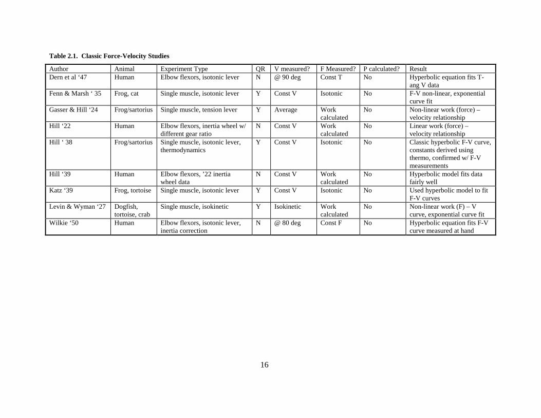
Table 2.1. Classic Force-Velocity Studies ....................................................................... 16
Table 2.2. Single Fiber Force-Velocity Studies ............................................................... 17
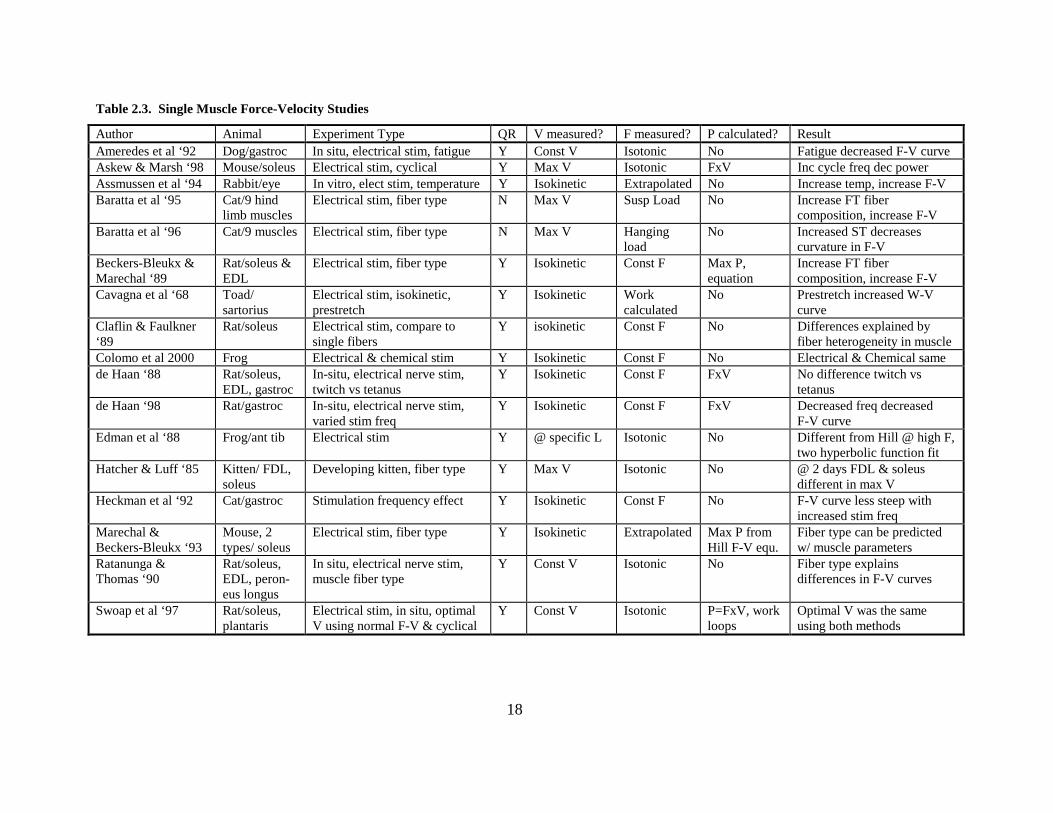
Table 2.3. Single Muscle Force-Velocity Studies............................................................ 18
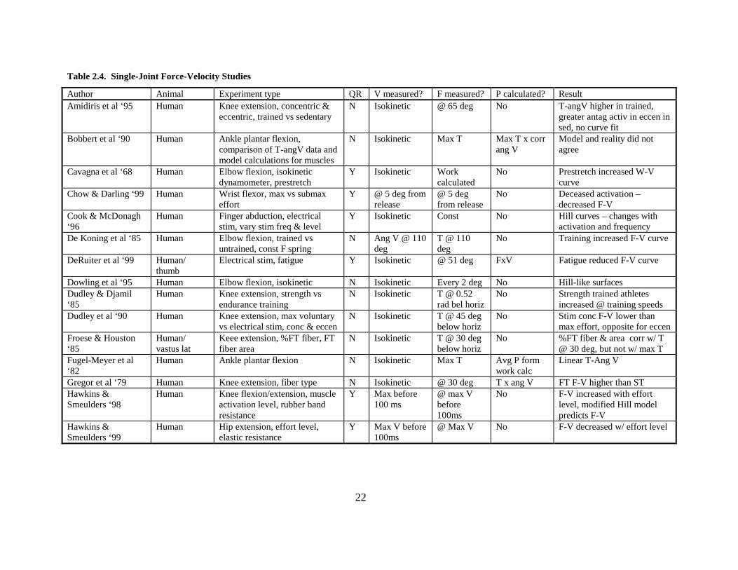
Table 2.4. Single-Joint Force-Velocity Studies ............................................................... 22
Table 2.5. Multi-Joint Force-Velocity Studies................................................................. 26
Table 3.1. Subject Data .................................................................................................... 34
Table 4.1. Hill’s constants for several variable combinations ......................................... 62
xi
Acknowledgements Completing a doctoral dissertation is a very challenging endeavor and cannot be
done alone; thus, I would like to individually recognize some of the people who were
instrumental in the completion of this work. This cannot be comprehensive and some
will invariably be missed, but some of the many important people are highlighted.
Many thanks go to the doctoral committee, Dr. Dick Nelson, my former advisor
before his retirement, Dr. Joe Sommer, my link to my engineering past, and Dr. Bill
Kraemer, the physiologist who has contributed greatly to my interests in his field. I could
not have completed the dissertation in the same way without their assistance and
guidance.
A special thanks goes to the chair of my committee, Dr. Vladimir Zatsiorsky. His
guidance and comments through the analyzing and writing processes were invaluable. I
am also grateful for his patience and understanding as my personal and professional
situations changed throughout the years.
Deep appreciation goes to the undergraduate interns and fellow graduate students
who all played an important part in carrying out this project, but especially Mike Pfaff,
who did most of the very boring job of digitizing the videotape of all of the trials with a
high level of enthusiasm. I would probably be still working on this project now if it were
not for his help. The engineering technicians, Joe Johnstonbaugh and Jeff Thompson,
deserve a large amount of credit for the design and construction of the impressive
apparatus for this study.
Appreciation goes to the subjects in this study, some of whom were members of
teams that I coached. I could not have had a project at all if it were not for them.
I could not leave out Harry Groves and Bill Whittaker, my fellow coaches with
the Penn State Track and Field Team, as well as the members of the teams during the
years that I both coached and worked on this project. They have no idea how much they
did to support my endeavors as I had to divide my time in several directions and to
constantly keep me excited about finishing this work.
All of my friends have contributed support and encouragement over the years, but
a few deserve special recognition. Matt Pain, a great friend and fellow graduate student,
xii
and Jeff Volek, with whom I lived in the same room for most of my time in graduate
school, always provided healthy diversions and set great examples on how to have fun
and still graduate. Robert Campbell, my University of Cincinnati engineering buddy and
best friend, is always there when I need him and consistently makes me feel like a
champion in whatever I am doing, no matter what the outcome.
I do not want to leave out my parents, Joel Hardyk and Lois Hernandez, who have
always been incredibly supportive of all of the endeavors in my life without ever pushing
too hard.
Finally, the most appreciation goes to my wife, Dr. Angela Hardyk. Angie has
been there for me in every possible situation and must have an infinite amount of
patience and understanding to put up with my endeavors as a coach, an athlete, and a
student, while at the same time completing her medical residency. No one will be more
excited than she that this project is finally done! Her love and support are beyond
compare and I feel I am the luckiest man alive to be married to her.
-Andrew Hardyk, October, 2000-

xiii
“It is odd how one’s brain fails to work
properly when pet theories are involved.”
- A.V. Hill, 1970 -

1
Chapter 1 Introduction
2
Everyday experience shows that as heavy objects are lifted, the speed of lifting is
slower than when lighter objects are lifted. Everyone intuitively knows about the
relationship between force and velocity. Force-velocity and power-velocity relationships
of skeletal muscle are popular topics in the fields of Biomechanics and Physiology.
Research began in earnest in the late 1920’s with studies completed by Hill (1922),
Gasser and Hill (1924), Levin and Wyman (1927), Fenn and Marsh (1935), Hill (1938),
and Katz (1939) and has continued into today’s current scientific literature. Study in this
field can be divided into four main areas: 1) classic studies, 2) single fiber/muscle
preparations in vitro, 3) single-joint studies in vivo, and 4) multi-joint studies.
A. V. Hill is perhaps the most famous researcher in this field. He and his team
were among the first to clearly define the force-velocity relationship in muscle. Using
muscle removed from amphibians, Hill determined that as the resistance against the
muscle increased, the contraction velocity decreased in a predictable, non-linear, concave
upward fashion. The now famous ‘Hill’s force-velocity equation’ was written to describe
the form of the displaced rectangular parabolic curve:
(V+b)(F+a)=(Fo+a)b=constant, (1)
where F is the external force on the muscle, V is the velocity of shortening, Fo is the
isometric tension, and a and b are constants. Nearly all scientists who have investigated
the force-velocity characteristics of muscle compared their results to this classic curve.
Researchers studying single fibers and muscles typically removed them from the
body of the animal and tested them using sophisticated equipment, which measured the
force produced by the muscle and the shortening velocity throughout a single muscular
action while keeping the velocity or the force constant. The muscles were maximally
stimulated either chemically or electrically, and the muscles were tested over a number of
trials against different loads. Research in this area has been diverse, and the effects of
many factors on the shape of the force-velocity curve have been studied. Topics have
included: fiber type (Baratta, et al., 1995; Bottinelli, et al., 1991), type of stimulation
(DeHaan, 1998; Heckman, et al., 1992), fatigue (Ameredes, et al., 1992; Curtin and
Edman, 1994; Lannergren and Westerblad, 1989), and temperature (Assmussen, et al.,
3
1994; Bottinelli, et al., 1996; Sobol and Nasledov, 1994). Animal muscles were the
primary models in this area of investigation. Nearly all researchers in this area have
compared their results to the Hill force-velocity curve and, with a few exceptions,
reported similar force-velocity curves.
Single-joint investigations have allowed for the study of human muscles and
involved one joint while the rest of the body was kept stationary during a maximum
effort. The force-velocity characteristics of the muscles or the torque-angular velocity
characteristics at the joint of interest were studied by either keeping the velocity of the
motion or the force against which the subject must move constant. The measurements
were taken at the instant of a maximum force, torque, or velocity, or at a specific joint
angle. There were two main joints investigated in the literature: the elbow (Dern, et al.,
1947; Wilkie, 1950; Cavagna, et al., 1968; Van Leemputte, et al., 1987; Martin, et al.,
1995), and the knee (Thorstensson, et al., 1976; Perrine and Edgerton, 1978; Johansson,
et al., 1987; Marshall et al., 1990; Ikegawa, et al., 1995; Seger and Throstensson, 2000),
but the wrist (Chow and Darling, 1999), the finger (Cook and McDonagh, 1996), the hip
(Hawkins and Smeulders, 1999), and the ankle (Bobbert, et al., 1990) have recently been
studied as well. In general, most of these studies claimed that the resulting force-
velocity, or torque-angular velocity, curves compared favorably to Hill’s force-velocity
curves.
Force-velocity characteristics in multi-joint movements have been relatively
unexplored compared to the single fiber/muscle and single-joint relationships. Many
authors have investigated the force-velocity relationship in cycling (e.g. Baron, et al.,
1999; Seck et al., 1995; Hautier, et al., 1996). Other models for study have included:
horizontal arm pulls (Grieve and van der Linden, 1986), rowing ergometer (Hartmann, et
al., 1993), bench throws (Newton, et al., 1997), weighted baseball bats (Bahill and
Karnavas, 1991), and weight lifting (Thomas, et al., 1996). The vertical jump has been
studied by several scientists (Tsarouchas and Klissouras, 1981; Bosco and Komi, 1979;
Viitasalo, 1985; Jaric, et al., 1986; Bobbert, et al., 1986). Changes in force and velocity
were produced by requiring the subjects to jump with additional loads, or by attaching the
subjects to a calibrated spring via a harness and pulley system to unload them
4
(Tsarouchas and Klissouras, 1981). Once again, the results were favorably compared to
previous work by Hill (1938) and other force-velocity investigators. However, there is a
gap in the force-velocity literature for the vertical jump because several of the studies
mentioned above had questionable methods or did not actually attempt to mathematically
fit Hill’s curve to their data, and none of them had very wide ranges of force and velocity.
Power-velocity relationships in muscle have not been discussed in the literature to
the same extent as force-velocity relationships. Several authors reported power-velocity
curves in single-joint investigations (e.g. Johansson, et al, 1987; Perrine and Edgerton,
1978; Gregor, et al., 1979; Fugel-Meyer, et al., 1982) using isokinetic dynamometry. The
main finding in these studies was that power increased with joint velocity, but the curve
began to level off at high velocities. Power-velocity curves seem to be rare in the
literature for multiple joint movements with the exception of studies involving cycle
ergometry (e.g. Baron, et al., 1999; Seck et al., 1995; Hautier, et al., 1996), but authors
often mention peak or average power (e.g. Cavagna, et al., 1971; Harman, et al., 1990;
Bartosiewicz, et al., 1990). Power was often reported in the vertical jumping literature as
a measure of athletic ability or as a predictor for vertical jumping ability (e.g. Aragon-
Vargas and Gross, 1997; Dowling and Vamos, 1993; Thomas, et al., 1996) and in
reference to individual muscle power (e.g. Voigt, et al., 1995; Jacobs, et al., 1996;
Bobbert, et al., 1986; Pandy and Zajac, 1991) and joint power (e.g. Prilutsky and
Zatsiorsky, 1994; Jacobs, et al., 1996; van Soest, et al., 1993; Gregoire, et al., 1984).
A similarity between all of the methods described above was that they were all
parametric, that is, a single instant in time was chosen during each trial for study and all
of the single points from each trial were combined to form one curve. A parameter of the
motor task was changed from trial to trial (e.g. the external load). However, there are
several significant differences between single fiber/muscle and single-/multi-joint force-
velocity studies. The velocity of shortening in the first class of experiments is normally
relatively constant for most of the shortening range. This means that it is not as
important at which point in the contraction history the velocity or force is measured. As
long as the velocity or force is not measured during the initial acceleration or the final
deceleration during the movement, the measurement will be accurate. Single-joint testing
5
has the intrinsic complication of non-constant force and velocity profiles due to
anatomical constraints. Multi-joint movement has the added complication that several
muscles are involved with the movement in addition to the fact that there are multiple
joints, all moving in an unknown coordination pattern. Therefore, the options when
deciding at which point to measure or analyze force and velocity are virtually limitless
and complicated to interpret.
The subjects in this study were asked to perform maximum-effort,
noncountermovement vertical jumps against loads that varied from trial to trial. The
subjects were loaded with a barbell and weights. The subjects were unloaded with
stretched elastic bands. The force-velocity and power-velocity relationships were studied
using force plate and video analyses and used the instant of maximum velocity as the
time at which the parameters were measured.
The theoretical shape of the force-velocity curve in an investigation such as this is
a curve that resembles the Hill curve, i.e. a descending, concave upward curve. As the
resistance is increased, the velocity of movement should decrease. An important
measurement in the study of Hill-like curves is the parameter a/Fo. Typically this
parameter is between zero and one in the literature. For the purposes of this study, Hill-
like curves were defined as follows:
1) Descending,
2) Concave upward,
3) Ratio of constants a/Fo between zero and one.
All curves that did not fit into this definition were rejected as Hill-like.
The theoretical power-velocity curve should look like an ascending-descending
parabolic shape with its peak somewhere in the middle of the velocity range. The entire
theoretical force and velocity ranges (zero velocity to very high velocity and maximum
load to zero load) was impossible to cover in this study because the amount of load that
would be needed would become dangerous to lift, and the unloading force would pull the
subject from the floor before a jump could be attempted. Therefore, the curves that were
produced were only a portion of the entire theoretical curve.
6
The main goals of this investigation were to:
1) Determine the general shape of the various force-velocity and velocity-
load curves for a noncountermovement vertical jump (see #2)
2) Compare several velocity and force combinations:
a) Maximum velocity of the center of mass vs. the corresponding
ground reaction force and external load.
b) Maximum angular velocity of the knee joint vs. the corresponding
ground reaction force, corresponding knee moment and external
load.
c) Maximum linear velocity of leg extension as measured by the
change in linear distance between the ankle and hip joints vs. the
corresponding ground reaction force, corresponding knee moment,
and external load.
3) Determine the general shape of the various power-velocity and power-load
curves:
a) Power, calculated by multiplying maximum center of mass
velocity and the corresponding ground reaction force.
b) Power, calculated by multiplying maximum leg extension velocity
and corresponding ground reaction force.
c) Power, calculated by multiplying maximum knee angular velocity
and the corresponding knee moment.
4) Since the power-velocity/force/load curves in this study did not cover the
complete theoretical range possible, determine whether this experiment
lies in the ascending or descending portion of the theoretical curves.
5) Determine the load and velocity at which maximum power is produced (if
possible, since maximum power may not be included in the range of data).
7
The hypotheses for the results of the tests that meet the above goals are:
1) The shape of all of the force-velocity curves will be similar in shape to the
Hill model for muscle force-velocity characteristics, i.e. they will be Hill-
like as strictly defined above.
2) All of the combinations for force-velocity relationships will be
comparable, i.e. they will have similar correlation coefficients.
3) The shape of all the power-velocity curves will be similar to the
theoretical power-velocity curve; i.e. it will be a parabolic ascending-
descending curve peaking between the maximum and minimum velocity.
4) The power-force and -load curves will be in the ascending portion of the
theoretical curve and the power-velocity curves will be in the descending
portion.
5) The peak power will occur at approximately 33% of the maximum load
and velocity (as determined by the self-reported maximum squat lift of the
subjects and the maximum velocity predicted by the data).
8
Chapter 2 Review of Literature
9
The force-velocity relationship in muscle has been a topic of intense research for
a number of years. This review covers the main types of force-velocity studies. It is
intended to be comprehensive of the field, but no claim is made that all force-velocity
studies are included. The main focus of the review is parametric studies in the concentric
range of force production.
2.1 Force-Velocity Relationships
There are two main types of force-velocity studies in the literature. The first is
single-trial studies and the second is multi-trial studies. The main focus of the review is
on the multi-trial studies since this project is in that area. However, it is important to
understand the difference between the two to avoid confusion.
2.1.1 Single-Trial Force-Velocity Experiments
The idea behind this type of research is simple; the researcher measures the force
and the velocity concurrently and continuously during a trial. This can be accomplished
using a number of experimental models such as a single muscle fiber or whole muscle
preparation in vitro, or during a controlled movement using some sort of an animal
model.
There is a relatively small amount of research that uses this approach for the
specific purpose of measuring force-velocity relationships. van Ingen Schenau, et al.
(1985) used video and force plate data with an inverse dynamics approach to study the
torque-angular velocity characteristics of the ankle joint during a vertical jump. Komi, et
al. (1990) used a buckle-type force transducer temporarily implanted directly into the
achilles tendon of human subjects to measure force and used video data and muscle
modeling to calculate muscle shortening velocity during walking, running, and jumping.
The results from both of these studies were similar and were manifested in a force-
velocity relationship that was somewhat circular in shape. The results of these studies are
typical of other single-trial studies.
The point of mentioning these types of studies is that the force-velocity
relationship during a single trial is different than when multiple trials are presented in a
parametric way and does not strictly follow the famous force-velocity curves that are
10
commonly found in the literature. One of the common explanations for the differences in
these types of studies is that during in vivo testing, none of the variables (activation
levels, force, velocity, etc.) are held constant, whereas in parametric force-velocity
experiments, some part of the experiment is controlled. In other words the two
experiment types are different and have different results. Another possible reason for the
differences in the results is that in vivo testing includes all of the energy-storing
connective tissue, but in parametric tests, this tissue is often removed (Komi, et al.,
1990).
2.1.2 Multi-Trial Force-Velocity Experiments
The bulk of the force-velocity literature uses a multiple trial approach to study the
force-velocity relationship in muscle. In general, this involves a procedure where the
force and velocity are measured at a specific position or specific instant in the movement
during a single trial. One of the parameters of the experiment, i.e. external load, velocity
of shortening, etc., is then changed and the experiment is repeated. The single force-
velocity point from each trial is then plotted on one graph to produce a ‘parametric’
relationship for force and velocity (Zatsiorsky, 1995). This type of experiment has been
performed on a variety of muscle models including isolated animal and human muscle
fibers, whole muscle preparations in vitro and in situ for both animals and humans, and
human in vivo single-joint and multi-joint models. All of these models will be discussed
in detail.
Parametric force-velocity experiments typically attempt to control (keep
‘constant’) either the force that the fiber/muscle/subject is required to move against or the
velocity at which the fiber/muscle/subject will move during the trial. The other variable
is then measured at some time during the movement. Holding the force constant has been
attempted by subjecting the fiber/muscle/subject to a constant external load such as a
hanging weight or a barbell. Another method uses special equipment, called an isotonic
dynamometer, which has been designed to maintain constant resistance levels during a
movement. Holding velocity constant is usually accomplished using an isokinetic
dynamometer. This is a machine designed to absorb all of the energy produced in the
11
movement that would normally cause acceleration, thereby keeping the velocity at a
constant level.
In reality, none of these techniques perfectly maintains constant force or velocity.
In every experiment, the fiber/muscle/subject starts in a stationary position with no force
applied and then accelerates to a ‘constant’ state. This situation can be troublesome
because the acceleration period at low loads and/or high velocities can sometimes take up
the entire time of the movement. To overcome this problem, many experiments use the
so called ‘quick release’ method where the fiber/muscle/subject is allowed to build up
maximum isometric force at the beginning position of the movement and is then suddenly
released to the desired force or velocity level. Another potential problem is the inertia of
the apparatus and/or the fiber/muscle/subject itself. When the movement is produced in a
plane where gravity has an effect (e.g. seated leg extension), the actual forces/moments
measured will include the intrinsic force/moment produced against the load (isotonic) or
at the controlled velocity (isokinetic) and the force needed to lift and/or accelerate the
mass of the limb/apparatus. This problem can be corrected for mathematically or
experimentally. Correction for inertial properties is important when comparing the
results for different protocols, i.e. comparing isolated muscle preparations in vitro to
isotonic elbow flexions in vivo (Wilkie, 1950).
Since the force-velocity relationship is built up from multiple trials and only one
moment in time from each trial is used, the researcher must choose a time in the
movement to record the data. There are an infinite number of possibilities for this choice
and the literature reflects this variability. Some protocols have the advantage of having a
significant period of constant force and velocity during the movement. In these cases, the
specific time that the variables are measured is not critical as long as the measurements
occur during the constant periods. Most protocols do not have this luxury. Even if force
or velocity is held constant as the independent variable, the dependent variable is often
not constant over the range of movement, especially in experiments involving one or
more joints in human subjects. Even if the external load is held constant, the researcher
may be interested in the actual force and velocity produced, neither of which may be
constant throughout the range of movement (e.g. multi-joint movement against a constant
12
external load). Therefore, in these cases, the dependent variable(s) must be measured
either continuously, at a specific position in the movement, or at a specific moment in
time (i.e. time when maximum velocity or force occurs). The choices of time made for
measuring the force and velocity can have an effect on the interpretation of the results
and may have ramifications on how comparable individual studies may be.
The muscle activation level in these experiments is typically assumed to be
maximal. This means that in the in vitro fiber/muscle preparations the muscle is
maximally stimulated either chemically or electrically and in the in vivo human trials
maximum effort is produced. Recently there has been some effort to determine the force-
velocity relationship of submaximal efforts (Chow and Darling, 1999; Hawkins and
Smeulders, 1998, 1999).
Regardless of the protocol, the results of nearly all of these types of experiments
have been very similar. As velocity of movement increased, the force that was produced
in a maximal contraction decreased in a non-linear way. This has become known as the
famous force-velocity relationship (often called Hill’s curve, after A. V. Hill, see below)
and it seems to hold up under a wide variety of parametric protocols.
Researchers have also studied the force-velocity relationship in the eccentric
range of the force-velocity curve, i.e. when the force is so high that the muscle is
extended instead of shortened (Katz, 1939; Granzier, et al., 1989; Dudley, et al., 1990;
Kues and Mayhue, 1996; Seger and Thorstensson, 2000; Jorgensen, 1976; Amidiris, et
al., 1995). They found that Hill’s curve does not adequately describe the force-velocity
relationship during forced extension. The force increases very quickly flattens to a
constant value with increasing extension velocity. This area of research remains
relatively undefined because the force-velocity relationship has not been explored to a
great extent and because the properties for lengthening muscle are not as consistent or
easy to measure compared to shortening muscle (Epstein and Herzog, 1998).
2.1.3 Types of Multi-Trial Force-Velocity Experiments
As mentioned above, there are four main models for parametric force-velocity
experiments: single muscle fiber preparations in vitro, single muscle preparations in
vitro/in situ, single-joint in vivo, and multi-joint in vivo. Each type will be discussed
13
individually. Before that, a brief history of parametric force-velocity relationships will be
discussed in the form of a review of some of the classic early studies.
2.1.3.1 Classical Force-Velocity Studies
In 1922, A. V. Hill used a flywheel, a series of pulleys, and a hand held
tachometer to control and record the velocity when calculating the work done by the
elbow flexors during a simple, single-joint movement at the elbow. Maximum force
pulls on a string wrapped around wheels of progressively smaller radii for each trial
connected to the flywheel produced a range of inertial resistances and thus, a range of
average angular velocities of movement of the forearm. The results indicated that as the
inertia increased, the velocity of the movement increased, and the work done by the
muscles decreased somewhat linearly. Since the movement was carried out over the
same distance in each trial, the same relationship follows for the force, i.e. as velocity of
movement increased, the force decreased. This relationship was attributed to viscous
properties of the muscle and was modeled as a spring in a viscous damping fluid.
Gasser & Hill (1924) attempted to confirm the linear work (force)-velocity
relationship using isolated frog sartorious muscles. They used a quick-release method
with a tension lever to calculate the average velocity and work done by the muscles
against various resistances. They found that the work again decreased as the contraction
velocity increased, but the resulting work-velocity curve was not linear but hyperbola-
like. The viscous spring model did not predict this result.
Levin and Wyman (1927) continued this line of research by developing an
isokinetic measuring device that measured the tension on dogfish muscles during
constant velocity contractions. They found similar, non-linear work-velocity curves as
Gasser and Hill (1924) and fit the curve using an exponential model based on a viscous
spring in series with another spring. This model explained the data well. Fenn and
Marsh (1935) corroborated this work with experiments using frog and cat muscles and an
isotonic lever system and for the first time produced the familiar force-velocity curve.
Using frog and toad sartorius muscles, Hill (1938) used the measurement of heat
liberated during muscular contractions to predict the force-velocity characteristics of
muscle. He used an isotonic lever system and maximally electrically stimulated the
14
muscles. Thermodynamic sensors were used to measure the amount of energy expended
by the muscle in the form of excess heat during the contraction. He found that the heat
energy produced by the muscle (in excess of maintenance heat) was proportional to the
velocity:
∆E=(a + F)V, (1)
where V is the shortening velocity, F is the suspended weight (i.e. force produced by the
muscle), and a is a constant. He also found that the liberated thermal energy was
proportional to the difference between the maximum isometric force produced by the
muscle and the muscle force produced during a specific trial:
∆E=b(Fo-F), (2)
where F is the shortening velocity, Fo is the maximum isometric force, and b is a
constant. Combining these equations led to a general equation describing the force-
velocity relationship of the muscle:
(F+a)V = b(Fo-F), (3)
This equation can be rewritten as:
(V+b) (F+a) = (Fo+a)b = constant. (4)
These equations determine the relationship between the muscular force and speed of the
contraction and are in the form of a displaced rectangular hyperbola. Another useful
form of the curve is:
(V/b+1)(F/Fo+a/Fo) = (1+a/Fo) = constant, (5)
where a/Fo = V/b are parameters that describe the amount of curvature of the hyperbola.
The force-velocity curve and the values for the constants were confirmed with
purely mechanical methods with no heat measurements by measuring the force and
velocity directly using the same isotonic lever (Hill, 1938; Katz, 1939). The hyperbolic
model also successfully explained the data of Fenn and Marsh (1935), Levin and Wyman
(1927), and Gasser and Hill (1924).
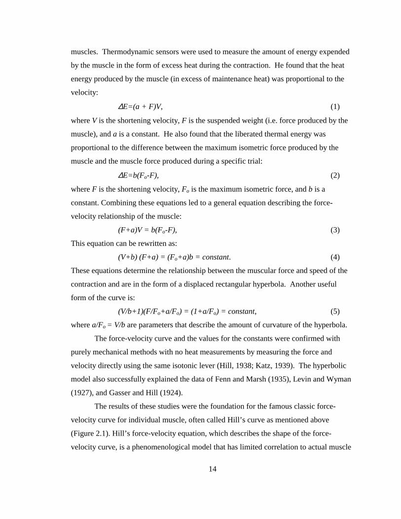
The results of these studies were the foundation for the famous classic force-
velocity curve for individual muscle, often called Hill’s curve as mentioned above
(Figure 2.1). Hill’s force-velocity equation, which describes the shape of the force-
velocity curve, is a phenomenological model that has limited correlation to actual muscle
15
FFo
V
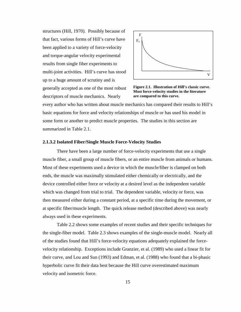
structures (Hill, 1970). Possibly because of
that fact, various forms of Hill’s curve have
been applied to a variety of force-velocity
and torque-angular velocity experimental
results from single fiber experiments to
multi-joint activities. Hill’s curve has stood
up to a huge amount of scrutiny and is
generally accepted as one of the most robust
descriptors of muscle mechanics. Nearly
every author who has written about muscle mechanics has compared their results to Hill’s
basic equations for force and velocity relationships of muscle or has used his model in
some form or another to predict muscle properties. The studies in this section are
summarized in Table 2.1.
2.1.3.2 Isolated Fiber/Single Muscle Force-Velocity Studies
There have been a large number of force-velocity experiments that use a single
muscle fiber, a small group of muscle fibers, or an entire muscle from animals or humans.
Most of these experiments used a device in which the muscle/fiber is clamped on both
ends, the muscle was maximally stimulated either chemically or electrically, and the
device controlled either force or velocity at a desired level as the independent variable
which was changed from trial to trial. The dependent variable, velocity or force, was
then measured either during a constant period, at a specific time during the movement, or
at specific fiber/muscle length. The quick release method (described above) was nearly
always used in these experiments.
Table 2.2 shows some examples of recent studies and their specific techniques for
the single-fiber model. Table 2.3 shows examples of the single-muscle model. Nearly all
of the studies found that Hill’s force-velocity equations adequately explained the force-
velocity relationship. Exceptions include Granzier, et al. (1989) who used a linear fit for
their curve, and Lou and Sun (1993) and Edman, et al. (1988) who found that a bi-phasic
hyperbolic curve fit their data best because the Hill curve overestimated maximum
velocity and isometric force.
Figure 2.1. Illustration of Hill’s classic curve. Most force-velocity studies in the literature are compared to this curve.
16
Table 2.1. Classic Force-Velocity Studies
Author Animal Experiment Type QR V measured? F Measured? P calculated? Result Dern et al ‘47 Human Elbow flexors, isotonic lever N @ 90 deg Const T No Hyperbolic equation fits T-
ang V data Fenn & Marsh ‘ 35 Frog, cat Single muscle, isotonic lever Y Const V Isotonic No F-V non-linear, exponential
curve fit Gasser & Hill ‘24 Frog/sartorius Single muscle, tension lever Y Average Work
calculated No Non-linear work (force) –
velocity relationship Hill ‘22 Human Elbow flexors, inertia wheel w/
different gear ratio N Const V Work
calculated No Linear work (force) –
velocity relationship Hill ‘ 38 Frog/sartorius Single muscle, isotonic lever,
thermodynamics Y Const V Isotonic No Classic hyperbolic F-V curve,
constants derived using thermo, confirmed w/ F-V measurements
Hill ‘39 Human Elbow flexors, ’22 inertia wheel data
N Const V Work calculated
No Hyperbolic model fits data fairly well
Katz ‘39 Frog, tortoise Single muscle, isotonic lever Y Const V Isotonic No Used hyperbolic model to fit F-V curves
Levin & Wyman ‘27 Dogfish, tortoise, crab
Single muscle, isokinetic Y Isokinetic Work calculated
No Non-linear work (F) – V curve, exponential curve fit
Wilkie ‘50 Human Elbow flexors, isotonic lever, inertia correction
N @ 80 deg Const F No Hyperbolic equation fits F-V curve measured at hand

17
Table 2.2. Single Fiber Force-Velocity Studies
Author Animal Experiment Type QR V measured? F Measured? P calculated? Result Bangart et al ‘97 Rat/soleus Effect of non-use & Ca++,
chemical stim Y Max V Isotonic Max P
Parabolic Eq. Non weight bearing decreased F-V & Ca++ use
Bottinelli et al ‘91 Rat/soleus EDL plantaris
Chemical stim, fiber type Y @ 30ms Isotonic FxV F-V can identify muscle type
Bottinelli et al ‘95 Rat/plantaris Chemical stim, light vs heavy myosin chains
Y @20ms Isotonic FxV Light myosin modulates V @ zero load only
Bottinelli et al ‘96 Human Chemical stim, fiber type, temperature
Y @ 20ms Isotonic FxV Increase FT fiber composition/temp, incr F-V,P
Curtin & Edman ‘94 Frog/ant tib Electrical stim, fatigue Y Const V Isotonic No Fatigue decreased F-V curve Granzier et al ‘89 Frog F-V & length, conc & eccen Y @ 3 diff L Isotonic No Linear, discontinuous @ V=0 Lannergren & Westerblad ‘89
Xenopus Electrical stim, fatigue, effect of caffeine & K+
Y Const V Isotonic FxV Caffeine aids recovery, K+ does not, not curve fitted
Lou & Sun ‘93 Frog/semi-tendinosis
Chemical stim, high load interest
Y Const V Isotonic No Bi-phasic F-V curve, fit using Hill’s & Edman’s curves
Malmqvist & Arner ‘96
Guinea pig/ taenia coli
Chemical stim, effect of Ca++ & okadaic acid
Y Const V Isotonic No Increased pCa++ & increased okadaic acid increased F-V
McDonald et al ‘94 Rat/soleus Chemical stim, effect of non-use
Y Const V Isotonic FxV Increased time of non-use decreased F-V curve
Sobol & Nasledov ‘94
Lamprey Electrical stim, temperature effects
Y Const V Isotonic No Increased temp decreased curvature & increased max V
Widrick et al ‘98 Human/ soleus
Chemical stim, effect of bed rest
Y Const V Isotonic From Hill’s F-V equation
Bed rest decreased F-V curve
18
Table 2.3. Single Muscle Force-Velocity Studies
Author Animal Experiment Type QR V measured? F measured? P calculated? Result Ameredes et al ‘92 Dog/gastroc In situ, electrical stim, fatigue Y Const V Isotonic No Fatigue decreased F-V curve Askew & Marsh ‘98 Mouse/soleus Electrical stim, cyclical Y Max V Isotonic FxV Inc cycle freq dec power Assmussen et al ‘94 Rabbit/eye In vitro, elect stim, temperature Y Isokinetic Extrapolated No Increase temp, increase F-V Baratta et al ‘95 Cat/9 hind
limb muscles Electrical stim, fiber type N Max V Susp Load No Increase FT fiber
composition, increase F-V Baratta et al ‘96 Cat/9 muscles Electrical stim, fiber type N Max V Hanging
load No Increased ST decreases
curvature in F-V Beckers-Bleukx & Marechal ‘89
Rat/soleus & EDL
Electrical stim, fiber type Y Isokinetic Const F Max P, equation
Increase FT fiber composition, increase F-V
Cavagna et al ‘68 Toad/ sartorius
Electrical stim, isokinetic, prestretch
Y Isokinetic Work calculated
No Prestretch increased W-V curve
Claflin & Faulkner ‘89
Rat/soleus Electrical stim, compare to single fibers
Y isokinetic Const F No Differences explained by fiber heterogeneity in muscle
Colomo et al 2000 Frog Electrical & chemical stim Y Isokinetic Const F No Electrical & Chemical same de Haan ‘88 Rat/soleus,
EDL, gastroc In-situ, electrical nerve stim, twitch vs tetanus
Y Isokinetic Const F FxV No difference twitch vs tetanus
de Haan ‘98 Rat/gastroc In-situ, electrical nerve stim, varied stim freq
Y Isokinetic Const F FxV Decreased freq decreased F-V curve
Edman et al ‘88 Frog/ant tib Electrical stim Y @ specific L Isotonic No Different from Hill @ high F, two hyperbolic function fit
Hatcher & Luff ‘85 Kitten/ FDL, soleus
Developing kitten, fiber type Y Max V Isotonic No @ 2 days FDL & soleus different in max V
Heckman et al ‘92 Cat/gastroc Stimulation frequency effect Y Isokinetic Const F No F-V curve less steep with increased stim freq
Marechal & Beckers-Bleukx ‘93
Mouse, 2 types/ soleus
Electrical stim, fiber type Y Isokinetic Extrapolated Max P from Hill F-V equ.
Fiber type can be predicted w/ muscle parameters
Ratanunga & Thomas ‘90
Rat/soleus, EDL, peron-eus longus
In situ, electrical nerve stim, muscle fiber type
Y Const V Isotonic No Fiber type explains differences in F-V curves
Swoap et al ‘97 Rat/soleus, plantaris
Electrical stim, in situ, optimal V using normal F-V & cyclical
Y Const V Isotonic P=FxV, work loops
Optimal V was the same using both methods
19
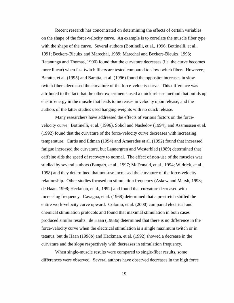
Recent research has concentrated on determining the effects of certain variables
on the shape of the force-velocity curve. An example is to correlate the muscle fiber type
with the shape of the curve. Several authors (Bottinelli, et al., 1996; Bottinelli, et al.,
1991; Beckers-Bleukx and Marechal, 1989; Marechal and Beckers-Bleukx, 1993;
Ratanunga and Thomas, 1990) found that the curvature decreases (i.e. the curve becomes
more linear) when fast twitch fibers are tested compared to slow twitch fibers. However,
Baratta, et al. (1995) and Baratta, et al. (1996) found the opposite: increases in slow
twitch fibers decreased the curvature of the force-velocity curve. This difference was
attributed to the fact that the other experiments used a quick release method that builds up
elastic energy in the muscle that leads to increases in velocity upon release, and the
authors of the latter studies used hanging weights with no quick release.
Many researchers have addressed the effects of various factors on the force-
velocity curve. Bottinelli, et al. (1996), Sobol and Nasledov (1994), and Assmussen et al.
(1992) found that the curvature of the force-velocity curve decreases with increasing
temperature. Curtis and Edman (1994) and Ameredes et al. (1992) found that increased
fatigue increased the curvature, but Lannergren and Westerblad (1989) determined that
caffeine aids the speed of recovery to normal. The effect of non-use of the muscles was
studied by several authors (Bangart, et al., 1997; McDonald, et al., 1994; Widrick, et al.,
1998) and they determined that non-use increased the curvature of the force-velocity
relationship. Other studies focused on stimulation frequency (Askew and Marsh, 1998;
de Haan, 1998; Heckman, et al., 1992) and found that curvature decreased with
increasing frequency. Cavagna, et al. (1968) determined that a prestretch shifted the
entire work-velocity curve upward. Colomo, et al. (2000) compared electrical and
chemical stimulation protocols and found that maximal stimulation in both cases
produced similar results. de Haan (1988a) determined that there is no difference in the
force-velocity curve when the electrical stimulation is a single maximum twitch or in
tetanus, but de Haan (1998b) and Heckman, et al. (1992) showed a decrease in the
curvature and the slope respectively with decreases in stimulation frequency.
When single-muscle results were compared to single-fiber results, some
differences were observed. Several authors have observed decreases in the high force
20
region of the force-velocity curve when compared to single fiber preparations (Edman, et
al., 1988). This was attributed to the elastic properties of the connective tissue of the
muscle. Another study (Claflin and Faulkner, 1989) indicated that differences in the
predicted maximum velocity were due to different muscle fiber types in the whole
muscle, compared to the single muscle fiber.
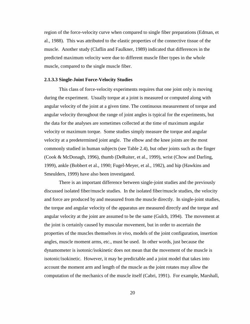
2.1.3.3 Single-Joint Force-Velocity Studies
This class of force-velocity experiments requires that one joint only is moving
during the experiment. Usually torque at a joint is measured or computed along with
angular velocity of the joint at a given time. The continuous measurement of torque and
angular velocity throughout the range of joint angles is typical for the experiments, but
the data for the analyses are sometimes collected at the time of maximum angular
velocity or maximum torque. Some studies simply measure the torque and angular
velocity at a predetermined joint angle. The elbow and the knee joints are the most
commonly studied in human subjects (see Table 2.4), but other joints such as the finger
(Cook & McDonagh, 1996), thumb (DeRuiter, et al., 1999), wrist (Chow and Darling,
1999), ankle (Bobbert et al., 1990; Fugel-Meyer, et al., 1982), and hip (Hawkins and
Smeulders, 1999) have also been investigated.
There is an important difference between single-joint studies and the previously
discussed isolated fiber/muscle studies. In the isolated fiber/muscle studies, the velocity
and force are produced by and measured from the muscle directly. In single-joint studies,
the torque and angular velocity of the apparatus are measured directly and the torque and
angular velocity at the joint are assumed to be the same (Gulch, 1994). The movement at
the joint is certainly caused by muscular movement, but in order to ascertain the
properties of the muscles themselves in vivo, models of the joint configuration, insertion
angles, muscle moment arms, etc., must be used. In other words, just because the
dynamometer is isotonic/isokinetic does not mean that the movement of the muscle is
isotonic/isokinetic. However, it may be predictable and a joint model that takes into
account the moment arm and length of the muscle as the joint rotates may allow the
computation of the mechanics of the muscle itself (Cabri, 1991). For example, Marshall,
21
et al. (1990) used x-rays of the knee in conjunction with isokinetic knee extensions to
create a model to calculate muscle forces and velocities.
Despite the above differences, force-velocity and torque-angular velocity plots for
single-joint movements tended to have a very similar shape as the single fiber/muscle
force-velocity plots. Numerous authors have reported Hill-like force-velocity and torque-
angular velocity curves in the literature. Exceptions include Kues and Mayhue (1996)
and Fugel-Meyer, et al. (1982) who used a linear fit to describe their data, and
Wakayama, et al. (1995) who used Fenn’s exponential equation to fit their data. In
addition, the torque-angular velocity curve was found to deviate from the force-velocity
curve predicted by Hill’s force-velocity equation and by isolated fiber/muscle data in the
high-torque range of the curve. At the lower angular velocities, the torque was not as
high as expected. This was postulated to be due to a central nervous system inhibition
designed to protect the muscles at high forces (Perrine and Edgerton, 1978; Kojima,
1991).
The most common approach by far to studying the force-velocity relationship for
the single-joint model has been isokinetic knee extension and flexion (Table 2.4). The
subject was strapped into the dynamometer in a seated position and the moving part of
the apparatus was strapped to the ankle. The center of rotation of the knee was aligned
with the rotation point of the apparatus. The subject then performed a series of maximum
effort full range of movement extensions or flexions at a predetermined set of angular
velocities. The torque was measured either by measuring the force exerted on the
dynamometer at the ankle and multiplying this by the length of the rotating arm of the
apparatus (tibia length) or directly at the rotation point of the dynamometer with sensors.
A similar approach was used for isokinetic studies of other joints.
Other researchers attempted to control the external force that the muscle had to
overcome in some fashion. Hanging weights (Wilkie, 1950; Kojima, 1991), elastic
resistance (Hawkins and Smeulders, 1998; 1999), a constant force spring (DeKoning, et
al., 1985) and changing the moment of inertia of the dynamometer (Tihyani, et al., 1982)
are all examples of this type protocol.
22
Table 2.4. Single-Joint Force-Velocity Studies
Author Animal Experiment type QR V measured? F measured? P calculated? Result Amidiris et al ‘95 Human Knee extension, concentric &
eccentric, trained vs sedentary N Isokinetic @ 65 deg No T-angV higher in trained,
greater antag activ in eccen in sed, no curve fit
Bobbert et al ‘90 Human Ankle plantar flexion, comparison of T-angV data and model calculations for muscles
N Isokinetic Max T Max T x corr ang V
Model and reality did not agree
Cavagna et al ‘68 Human Elbow flexion, isokinetic dynamometer, prestretch
Y Isokinetic Work calculated
No Prestretch increased W-V curve
Chow & Darling ‘99 Human Wrist flexor, max vs submax effort
Y @ 5 deg from release
@ 5 deg from release
No Deceased activation – decreased F-V
Cook & McDonagh ‘96
Human Finger abduction, electrical stim, vary stim freq & level
Y Isokinetic Const No Hill curves – changes with activation and frequency
De Koning et al ‘85 Human Elbow flexion, trained vs untrained, const F spring
N Ang V @ 110 deg
T @ 110 deg
No Training increased F-V curve
DeRuiter et al ‘99 Human/ thumb
Electrical stim, fatigue Y Isokinetic @ 51 deg FxV Fatigue reduced F-V curve
Dowling et al ‘95 Human Elbow flexion, isokinetic N Isokinetic Every 2 deg No Hill-like surfaces Dudley & Djamil ‘85
Human Knee extension, strength vs endurance training
N Isokinetic T @ 0.52 rad bel horiz
No Strength trained athletes increased @ training speeds
Dudley et al ‘90 Human Knee extension, max voluntary vs electrical stim, conc & eccen
N Isokinetic T @ 45 deg below horiz
No Stim conc F-V lower than max effort, opposite for eccen
Froese & Houston ‘85
Human/ vastus lat
Keee extension, %FT fiber, FT fiber area
N Isokinetic T @ 30 deg below horiz
No %FT fiber & area corr w/ T @ 30 deg, but not w/ max T
Fugel-Meyer et al ‘82
Human Ankle plantar flexion N Isokinetic Max T Avg P form work calc
Linear T-Ang V
Gregor et al ‘79 Human Knee extension, fiber type N Isokinetic @ 30 deg T x ang V FT F-V higher than ST Hawkins & Smeulders ‘98
Human Knee flexion/extension, muscle activation level, rubber band resistance
Y Max before 100 ms
@ max V before 100ms
No F-V increased with effort level, modified Hill model predicts F-V
Hawkins & Smeulders ‘99
Human Hip extension, effort level, elastic resistance
Y Max V before 100ms
@ Max V No F-V decreased w/ effort level
23
Table 2.4. Single-Joint Force-Velocity Studies (continued)
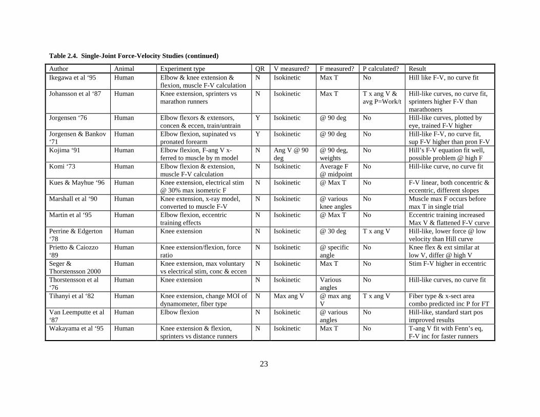
Author Animal Experiment type QR V measured? F measured? P calculated? Result Ikegawa et al ‘95 Human Elbow & knee extension &
flexion, muscle F-V calculation N Isokinetic Max T No Hill like F-V, no curve fit
Johansson et al ‘87 Human Knee extension, sprinters vs marathon runners
N Isokinetic Max T T x ang V & avg P=Work/t
Hill-like curves, no curve fit, sprinters higher F-V than marathoners
Jorgensen ‘76 Human Elbow flexors & extensors, concen & eccen, train/untrain
Y Isokinetic @ 90 deg No Hill-like curves, plotted by eye, trained F-V higher
Jorgensen & Bankov ‘71
Human Elbow flexion, supinated vs pronated forearm
Y Isokinetic @ 90 deg No Hill-like F-V, no curve fit, sup F-V higher than pron F-V
Kojima ‘91 Human Elbow flexion, F-ang V x-ferred to muscle by m model
N Ang V @ 90 deg
@ 90 deg, weights
No Hill’s F-V equation fit well, possible problem @ high F
Komi ‘73 Human Elbow flexion & extension, muscle F-V calculation
N Isokinetic Average F @ midpoint
No Hill-like curve, no curve fit
Kues & Mayhue ‘96 Human Knee extension, electrical stim @ 30% max isometric F
N Isokinetic @ Max T No F-V linear, both concentric & eccentric, different slopes
Marshall et al ‘90 Human Knee extension, x-ray model, converted to muscle F-V
N Isokinetic @ various knee angles
No Muscle max F occurs before max T in single trial
Martin et al ‘95 Human Elbow flexion, eccentric training effects
N Isokinetic @ Max T No Eccentric training increased Max V & flattened F-V curve
Perrine & Edgerton ‘78
Human Knee extension N Isokinetic @ 30 deg T x ang V Hill-like, lower force @ low velocity than Hill curve
Prietto & Caiozzo ‘89
Human Knee extension/flexion, force ratio
N Isokinetic @ specific angle
No Knee flex & ext similar at low V, differ @ high V
Seger & Thorstensson 2000
Human Knee extension, max voluntary vs electrical stim, conc & eccen
N Isokinetic Max T No Stim F-V higher in eccentric
Thorstensson et al ‘76
Human Knee extension N Isokinetic Various angles
No Hill-like curves, no curve fit
Tihanyi et al ‘82 Human Knee extension, change MOI of dynamometer, fiber type
N Max ang V @ max ang V
T x ang V Fiber type & x-sect area combo predicted inc P for FT
Van Leemputte et al ‘87
Human Elbow flexion N Isokinetic @ various angles
No Hill-like, standard start pos improved results
Wakayama et al ‘95 Human Knee extension & flexion, sprinters vs distance runners
N Isokinetic Max T No T-ang V fit with Fenn’s eq, F-V inc for faster runners
24
The force-velocity or torque-angular velocity curve has been investigated in
relation to a number of other single-joint variables. The force-velocity curve was shown
to have less curvature in subjects with higher percentages of fast-twitch fibers (Froese
and Houston, 1985; Tihanyi, et al., 1982; Gregor, et al., 1979), and similar results were
found when comparing sprinters and distance runners (Johansson, et al., 1987;
Wakayama, et al., 1995). Increased stimulation frequency (Cook and McDonagh, 1996),
increased training level (Dudley and Djamil, 1985; DeKoning et al., 1985; Martin, et al.,
1995; Jorgensen, 1976; Amidiris, et al., 1995), and prestretch (Cavagna, et al., 1968)
shifted the force-velocity curve upward, while fatigue (DeRuiter et al., 1999) shifted it
downward. Knee extension and flexion force-velocity curves had different slopes;
however similar force was observed at low velocities (Prietto and Caiozzo, 1989).
2.1.3.4 Multi-Joint Force-Velocity Studies
Experiments of this type include movements that involve multiple joints.
Examples of multi-joint systems are the arms/shoulder and the legs. Multiple muscles are
involved in these movements making the analysis much more complex. Similar to the
single joint protocol, multi-joint force-velocity studies require detailed joint models to
calculate forces and velocities of actual muscles during a movement.
There are a number of possible methods to measure both force and velocity. A
common protocol is to have the subject move against a constant external load or mass,
similar to previous types of protocols. Other possible methods include measuring the
force exerted on the load, the force at an endpoint of the system (e.g. ground reaction
force in a vertical jump), the torque produced at a joint, the calculation of the actual
muscle force, or average force or torque over the entire movement. Possible choices for
measuring the velocity include: the velocity of the center of mass of the system, the
velocity of an endpoint (e.g. velocity of the hand in an arm pull), the angular velocity of a
particular joint, or average velocity of any of the previous velocity options over the entire
movement.
A characteristic of multi-joint movements is that there often is no period of
constant force or velocity during the movement. This complicates the choice of the time
of measurement during the movement. Common choices were to measure both force and

25
velocity at the time of maximum velocity (Newton, et al., 1997) or angular velocity
(Bosco and Komi, 1979), or at a specific position (Grieve and van der Linden, 1986) or
joint angle (Bahill and Karnavas, 1991; Kunz, 1974; Jaric, et al., 1986). Another
common technique was to average force and velocity over the entire movement
(Viitasalo, 1985; Bosco and Komi, 1979; Newton, et al., 1997). There are virtually an
infinite number of possibilities and the literature reflects this. The variability of these
choices can affect the interpretation of the results of a study and can influence the
comparability of the results of different protocols.
There are many examples of multi-joint force-velocity studies (Table 2.5). One of
the most common was the use of a cycle ergometer or stationary bicycle. The hips,
knees, and ankle were free to move in these studies but the feet were typically strapped to
the pedals and the subject was required to remain seated at all times during a trial. There
are two types of protocols in force-velocity testing on a cycle ergometer, single-trial
(Baron, et al., 1999; Buttelli, et al., 1999, 1997, 1996; Capmal and Vandewalle, 1997;
Seck, et al., 1995; Hautier, et al., 1996; Arsac, et al., 1995) and multi-trial (Baron, et al.,
1999; Driss, et al., 1998; Jaskolska, et al., 1999; Linossier, et al., 1996; Vandewalle, et
al., 1987). In the single trial protocol, the subject performed a single maximal sprint from
zero revolutions per minute to the subject’s maximum speed against a constant resistance.
The torque exerted on the crank and pedal frequency was measured once during each
revolution of the pedals, or the torque and velocity was averaged for each revolution of
the pedals. The torque and its corresponding rotation speed were then plotted
parametrically. The multi-trial protocol required that the subject pedal at maximum
speed against several braking forces, one braking force for each trial. The maximum
pedaling speed during each trial was plotted against the braking force or the maximum
torque. Both of these protocols produced a linear torque-angular velocity relationship
with negative slope. In fact Seck, et al. (1995) found that the curves were nearly the
same for both protocols. The results on cycle ergometry had a vague resemblance to
Hill’s relationship in that as the pedaling speed increased, torque decreased, but since it
was a linear relationship, a curve as complex as Hill’s was not needed.
26
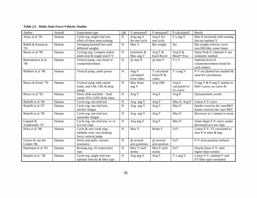
Table 2.5. Multi-Joint Force-Velocity Studies
Author Animal Experiment type QR V measured? F measured? P calculated? Result Arsac et al ‘95 Human Cycle erg, single trial rest,
effect of short term training N Avg ang V
for one cycle Avg F for one cycle
F x ang V Max P increased with training but not optimal V
Bahill & Karnavas ‘91
Human Swinging baseball bat with different weights
N Max V Bat weight No Bat weight-velocity curve was Hill-like, some linear
Baron et al ‘99 Human Cycling erg, Compare isokin multi-trial & single trial F-V
N Isokinetic & Max ang V
Avg T & Each Revol
Avg P & MaxP=Txw
Same Peak P, Optimal V use isokinetic method
Bartosiewicz et al ‘90
Human Vertical jump, vary level of countermovement
N @ max P @ max P F x V Optimal level of countermovement found for each subject
Bobbert et al ‘86 Human Vertical jump, ankle power N Ang V calculated from video
T calculated from FP & video
T x ang V F-V not plotted but implied & used for calculations
Bosco & Komi ‘79 Human Vertical jump with varied loads, non CM, CM, & drop jumps
N Max Knee ang V
Avg GRF Avg P, calculated w/ F-t curve
F-ang V & P-ang V similar to Hill’s curve, no curve fit
Bosco et al ‘95 Human Horiz slide machine – load varies 35%-210% body mass
N Avg V Avg F Avg P Dynamometer works
Buttelli et al ‘96 Human Cycle erg, one trial test N Avg ang V Avg T Max P, Avg P Linear F-V curve Buttelli et al ‘97 Human Cycle erg, one trial test,
aerobic fatigue N Avg ang V Avg T Max P Harder exercise dec maxP&V
Easier exercise dec max P&T Buttelli et al ‘99 Human Cycle erg, one trial test,
anaerobic fatigue N Avg ang V Avg T Max P Recovery in 1 minute to norm
Capmal & Vandewalle ‘97
Human Cycle erg, one trial test, w/ vs w/o toe clips
N Avg ang V Avg T Max P Same shape F-V curve, peaks decreased w/o toe clips
Driss et al ‘98 Human Cycle & arm crank ergs, multiple trial, vary braking force, vertical jump
N Max V Brake F FxV Linear F-V, VJ correlated to max P in arms & legs
Grieve & van der Linden ‘86
Human Horiz arm pulls, viscous resistance
N @ several arm positions
@ several arm position
FxV F-V-Arm position surfaces
Hartmann et al ‘93 Human Rowing erg, 10 consecutive reps
N Max V each stroke
Max F each stroke
FxV Nearly linear F-V, men higher than women
Hautier et al ‘ 96 Human Cycle erg, single trial test, optimal velocity & fiber type
N Avg ang V Avg T T x ang V Linear F-V, optimal V and FT fiber type correlated
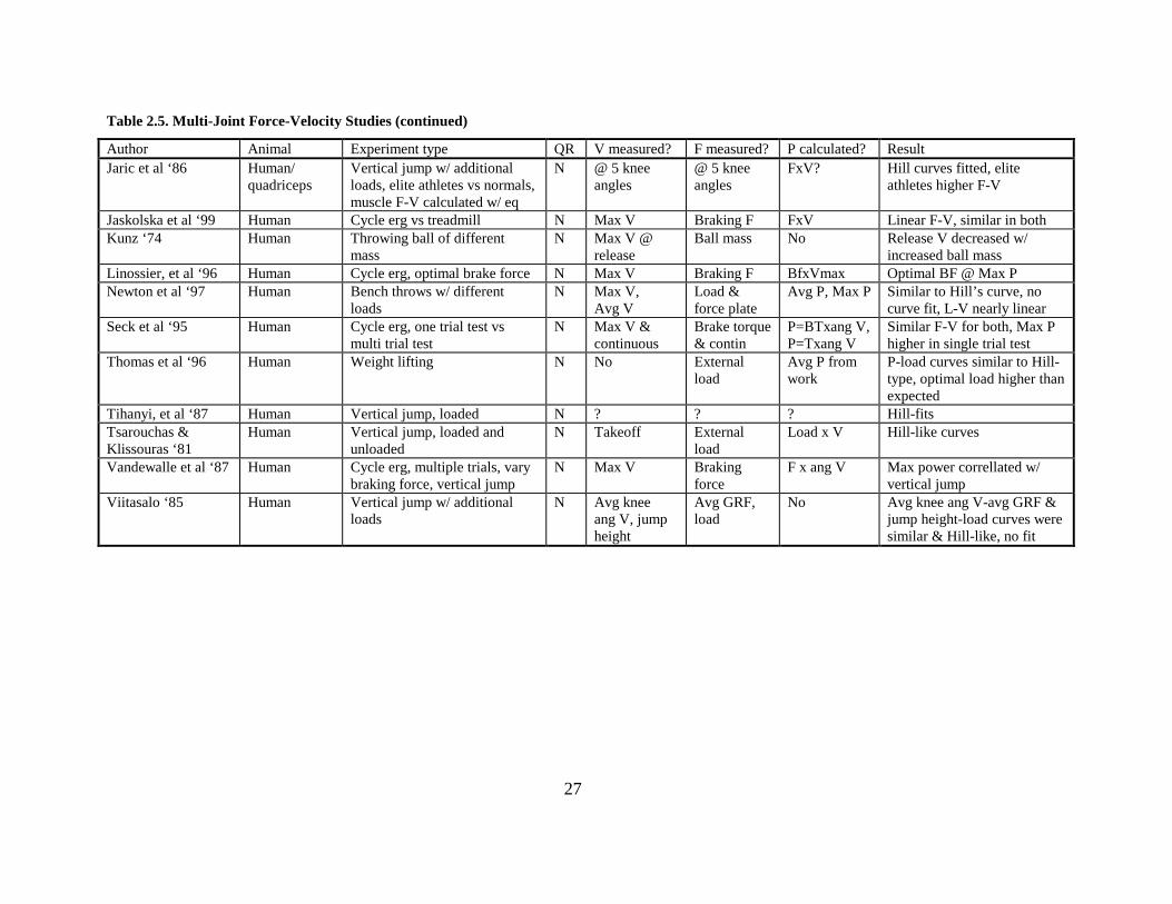
27
Table 2.5. Multi-Joint Force-Velocity Studies (continued)
Author Animal Experiment type QR V measured? F measured? P calculated? Result Jaric et al ‘86 Human/
quadriceps Vertical jump w/ additional loads, elite athletes vs normals, muscle F-V calculated w/ eq
N @ 5 knee angles
@ 5 knee angles
FxV? Hill curves fitted, elite athletes higher F-V
Jaskolska et al ‘99 Human Cycle erg vs treadmill N Max V Braking F FxV Linear F-V, similar in both Kunz ‘74 Human Throwing ball of different
mass N Max V @
release Ball mass No Release V decreased w/
increased ball mass Linossier, et al ‘96 Human Cycle erg, optimal brake force N Max V Braking F BfxVmax Optimal BF @ Max P Newton et al ‘97 Human Bench throws w/ different
loads N Max V,
Avg V Load & force plate
Avg P, Max P Similar to Hill’s curve, no curve fit, L-V nearly linear
Seck et al ‘95 Human Cycle erg, one trial test vs multi trial test
N Max V & continuous
Brake torque & contin
P=BTxang V, P=Txang V
Similar F-V for both, Max P higher in single trial test
Thomas et al ‘96 Human Weight lifting N No External load
Avg P from work
P-load curves similar to Hill-type, optimal load higher than expected
Tihanyi, et al ‘87 Human Vertical jump, loaded N ? ? ? Hill-fits Tsarouchas & Klissouras ‘81
Human Vertical jump, loaded and unloaded
N Takeoff External load
Load x V Hill-like curves
Vandewalle et al ‘87 Human Cycle erg, multiple trials, vary braking force, vertical jump
N Max V Braking force
F x ang V Max power correllated w/ vertical jump
Viitasalo ‘85 Human Vertical jump w/ additional loads
N Avg knee ang V, jump height
Avg GRF, load
No Avg knee ang V-avg GRF & jump height-load curves were similar & Hill-like, no fit
28
Bahill and Karnavas (1991) measured velocity as baseball players swung baseball
bats of differing weights, and Kunz (1974) measured the speed of release as subjects
threw balls of differing mass. Both authors found that the speed of the implements
decreased with increasing weight or mass, and the velocity of the baseball bat decreased
in a Hill-like manner that could be described with a hyperbolic curve fit. In a related
study, Newton, et al. (1997) studied the load-velocity relationship in bench press throws.
The results showed a nearly linear, but Hill-like relationship. Two additional upper body
experiments (Grieve and van der Linden, 1986; Hartmann, et al., 1993) showed Hill-like
force-velocity relationships for pulls against viscous resistance and for repetitive strokes
on a rowing ergometer respectively. Both of these studies measured the force and
velocity at the hand grip.
The final group of experiments under review for studying multi-joint force-
velocity relationships used the vertical jump as the multi-joint model. Bosco and Komi
(1979) compared the results of noncountermovement, countermovement and drop vertical
jumps with different additional loads placed on the shoulders of the subjects with a
barbell for each jump. The maximum angular velocity of the knee joint was plotted
parametrically against the average ground reaction force. The resulting curves were
found to be Hill-like but no curve was fit to the data. The ground reaction force was
assumed to be a direct result of the action of the knee extensors, as was the knee angular
velocity, similar to isokinetic leg extensions. Since no joint model was used, the validity
of these results could be questioned. In a similar study, Viitasalo (1985) plotted average
knee angular velocity vs. average ground reaction force during loaded vertical jumps, as
well as the height of the vertical jump vs. the additional load. Both curves were found to
be Hill-like, but no curves were fit to the data.
Jaric, et al. (1986) accomplished a vertical jump study where elite and untrained
subjects jumped against additional resistance. A joint model was used to calculate the
force and velocity produced in the quadriceps and measured at five joint angles.
However, this model did not include the any moment arm calculations, it seemed to be
merely a phenomenological conversion model. Hill’s curve was fitted to the resulting
force-velocity data, with the force-velocity of the elite subjects above the untrained
29
subjects. Tihanyi, et al. (1987) fit loaded vertical jump force-velocity data with Hill’s
curve, but did not report which specific forces or velocities were used. They determined
that at least four data points are required to properly fit Hill’s curve as long as the range
of forces used is at least 15 to 100% of the maximum isometric force.
Attempting to increase the range of the force-velocity curve in vertical jumping,
Tsarouchas and Klissouras (1981) used loaded and unloaded vertical jumps. The extra
load was provided with bags filled with sand on the shoulders, and the unloaded
conditions were accomplished using a calibrated spring, harness, and pulley system.
External load was plotted parametrically with takeoff velocity, producing Hill-like curves
that were not mathematically fit to the data. However, they did not measure the actual
force of unloading throughout the jump, only the average unloading force as calculated
from the calibrated spring. This may have caused inaccuracies in the velocity
calculations (the values for velocity were very high). They also reported the unusual
result that maximum ground reaction force did not continue to decrease with increased
unloading and did not increase above 150% of body weight loading. This may indicate a
problem with the experimental protocol or the physical abilities of their subjects.
Bosco, et al. (1995) used a horizontal slide machine connected to a weight stack
to validate a dynamometer for evaluating human performance using a jumping style
protocol. The range of loads was 35% to 210% of body weight. Average force and
velocity were reported and produced linear force-velocity relationships when combined
parametrically. This method appears to have potential for use in future force-velocity
research.
There appears to be a gap in the literature in the force-velocity relationship for
vertical jumping. Many of the relevant variables such as ground reaction force, knee
torque, maximum knee angular velocity, and maximum center of mass velocity have not
been addressed sufficiently. In addition, some of the methods for measurement and
analysis could be questioned. The force and velocity ranges in vertical jump studies have
been very limited for the most part; therefore, the vertical jump model has not been
sufficiently researched. This is a very commonly used movement in sport and science
and deserves more attention.
30
2.2 Power-Velocity and Power-Force Relationships
The relationship between power and velocity and/or force is an interesting way to
examine the force-velocity relationship from another point of view. Power has been
associated with many positive attributes of athletics and the performance of explosive
movements including the vertical jump (e.g. Dowling and Vamos, 1993). Therefore, it is
natural that study into the production of power produced in muscle would be of interest to
scientists and athletes. For the purposes of this review, all references to power are in the
context of the force-velocity curve unless mentioned specifically in the text.
Power is most often calculated using the product of each force and velocity pair in
the parametric force-velocity relationship. Each individual point can then be plotted
against either force or velocity, depending on the interests of the individual study (see
Tables 2.2-2.5). Average power was sometimes reported in the literature as the work
produced in a movement divided by the time of the movement for each trial (Thomas, et
al., 1996; Fugel-Meyer, et al., 1982; Johansson, et al., 1987; Bosco and Komi, 1979).
Both methods usually result in a parabolic-shaped curve (Epstein and Herzog, 1998).
The choice of the specific force and velocity variables and the choice of the time
where they are measured in the movement can make the calculation of power complex,
especially in the case of multi-joint movements. For example, the corresponding ground
reaction force in a vertical jump could be multiplied by the takeoff velocity or the
maximum velocity; the maximum ground reaction force or the maximum knee torque
could be multiplied by the corresponding angular velocity of the knee. Power
calculations in single joint/fiber studies are much simpler since there are fewer choices
for force and velocity.
Many authors were interested in the maximum power point of the curve. When
the force-velocity relationship was linear, such as in cycle ergometer studies, the
maximum power was easily calculated as the product of 0.5 × maximum force and 0.5 ×
maximum velocity, which equals 0.25 × maximum force × maximum velocity (Buttelli,
et al., 1999, 1997, 1996; Capmal and Vanderwalle, 1997). The velocity or force where
parametric power was maximal was also a common source of interest (Swoap, et al.,
1997; Baron, et al., 1999; Newton, et al., 1997; Arsac, et al., 1995; Thomas, et al., 1996).
31
The value of optimal velocity and force, i.e. the force and velocity where power was
maximal, has been reported to be approximately 0.33 × maximum force and 0.33 ×
maximum velocity (Newton, et al., 1997; Kraemer and Newton, 1994). However,
Thomas, et al. (1996) found that the force where maximum power occurred in weight
lifting was somewhat higher.
Power was used in conjunction with the force-velocity relationship to analyze
many of the same variables mentioned above for single fiber/muscle preparations, single-
joint studies, and multi-joint studies. Examples include: fiber type, temperature, fatigue,
non-use, electrical cycling frequency, comparison of protocol, training effects, and level
of countermovement. Please see Tables 2.2-2.5 for specific references. There appears to
be very little or no research in the area of power in the eccentric range of the force-
velocity relationship.
2.3 Conclusion
The force-velocity relationship of muscle is well known and has received
considerable attention in the literature. The concentric portion of the curve is the best
defined because of the ease of measurement and consistency of the results. The eccentric
portion of the curve is less defined because of a distinct lack of research in the area and
the difficulty in producing consistent and reliable results.
Nearly all researchers either compared their results to or used the results of Hill
and his hyperbolic equation for the force-velocity relationship. This is a descriptive
equation that has little direct correlation to actual muscle properties or structure.
However, the curve seemed to adequately describe the mechanics of muscle in many
situations from single fiber studies to multi-joint studies. Power-velocity and power-
force relationships are another common way to express and analyze muscle mechanics.
There appeared to be a gap in the literature for well-done multi-joint studies with
a wide range of forces and velocities. This was the focus of this study.
32
Chapter 3 Methods
33
This chapter outlines the experiment, the experimental protocol, and the methods
for analysis. A set of pilot experiments also was performed. A brief description of these
experiments and their influence on the current study can be found in the Appendix.
3.1 Subjects
Ten well-trained athletic males between the ages of 19 and 29 selected from Penn
State University athletic teams and graduate school served as subjects for this
experiment. The experimental protocol was explained to all of the subjects and all of
them signed an informed consent form reviewed and approved by the Penn State
University Office of Regulatory Compliance. When possible, they were chosen for their
ability in jumping- or power-type events because of the explosive nature of the
experiment. This was determined mainly by their sport and/or event in their sport.
The subjects were identified only by a letter or a number (e.g. subject A, B, C…
or subject 1, 2, 3…). The best performance of each subject in their sport was recorded as
well as their height, weight, best vertical jump, and best lift in the squat exercise (Table
3.1). The squat parameter was needed to determine if the subject could easily perform a
squat with a weight equal to their body weight. Sufficient experience and training was
important for the safety of the subjects and to produce a wide range of experimental data.
The athlete was not chosen if sufficient experience and ability were not demonstrated.
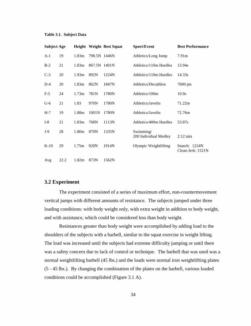
34
Table 3.1. Subject Data
Subject Age Height Weight Best Squat Sport/Event Best Performance A-1 19 1.83m 798.5N 1446N Athletics/Long Jump 7.91m B-2 21 1.83m 867.5N 1401N Athletics/110m Hurdles 13.94s C-3 20 1.93m 892N 1224N Athletics/110m Hurdles 14.33s D-4 20 1.83m 862N 1847N Athletics/Decathlon 7600 pts F-5 24 1.73m 781N 1780N Athletics/100m 10.9s G-6 21 1.83 970N 1780N Athletics/Javelin 71.22m H-7 19 1.88m 1001N 1780N Athletics/Javelin 72.76m I-8 21 1.83m 768N 1113N Athletics/400m Hurdles 53.87s J-9 28 1.80m 870N 1335N Swimming/
200 Individual Medley 2:12 min K-10 29 1.75m 920N 1914N Olympic Weightlifting Snatch: 1224N
Clean-Jerk: 1521N Avg 22.2 1.82m 873N 1562N
3.2 Experiment
The experiment consisted of a series of maximum effort, non-countermovement
vertical jumps with different amounts of resistance. The subjects jumped under three
loading conditions: with body weight only, with extra weight in addition to body weight,
and with assistance, which could be considered less than body weight.
Resistances greater than body weight were accomplished by adding load to the
shoulders of the subjects with a barbell, similar to the squat exercise in weight lifting.
The load was increased until the subjects had extreme difficulty jumping or until there
was a safety concern due to lack of control or technique. The barbell that was used was a
normal weightlifting barbell (45 lbs.) and the loads were normal iron weightlifting plates
(5 - 45 lbs.). By changing the combination of the plates on the barbell, various loaded
conditions could be accomplished (Figure 3.1 A).
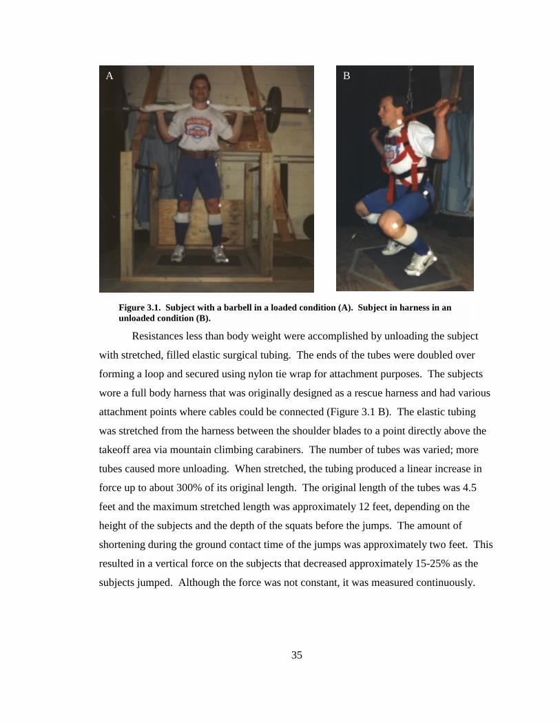
35
Resistances less than body weight were accomplished by unloading the subject
with stretched, filled elastic surgical tubing. The ends of the tubes were doubled over
forming a loop and secured using nylon tie wrap for attachment purposes. The subjects
wore a full body harness that was originally designed as a rescue harness and had various
attachment points where cables could be connected (Figure 3.1 B). The elastic tubing
was stretched from the harness between the shoulder blades to a point directly above the
takeoff area via mountain climbing carabiners. The number of tubes was varied; more
tubes caused more unloading. When stretched, the tubing produced a linear increase in
force up to about 300% of its original length. The original length of the tubes was 4.5
feet and the maximum stretched length was approximately 12 feet, depending on the
height of the subjects and the depth of the squats before the jumps. The amount of
shortening during the ground contact time of the jumps was approximately two feet. This
resulted in a vertical force on the subjects that decreased approximately 15-25% as the
subjects jumped. Although the force was not constant, it was measured continuously.
Figure 3.1. Subject with a barbell in a loaded condition (A). Subject in harness in an unloaded condition (B).
A B
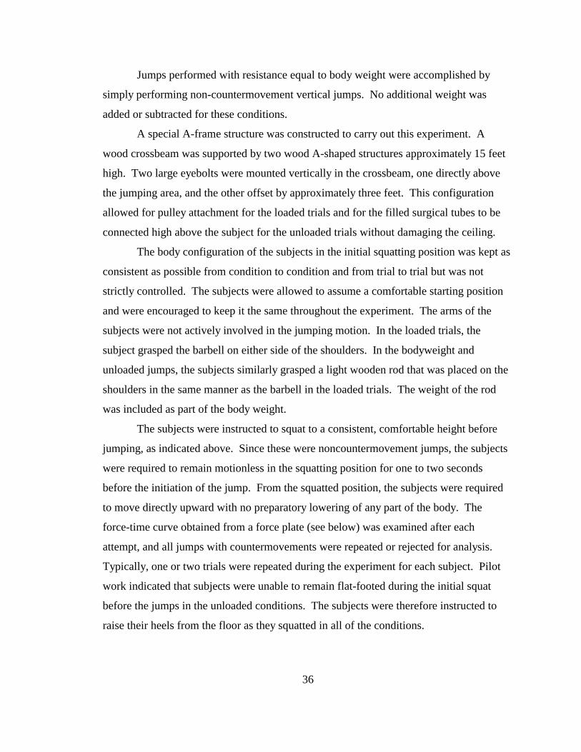
36
Jumps performed with resistance equal to body weight were accomplished by
simply performing non-countermovement vertical jumps. No additional weight was
added or subtracted for these conditions.
A special A-frame structure was constructed to carry out this experiment. A
wood crossbeam was supported by two wood A-shaped structures approximately 15 feet
high. Two large eyebolts were mounted vertically in the crossbeam, one directly above
the jumping area, and the other offset by approximately three feet. This configuration
allowed for pulley attachment for the loaded trials and for the filled surgical tubes to be
connected high above the subject for the unloaded trials without damaging the ceiling.
The body configuration of the subjects in the initial squatting position was kept as
consistent as possible from condition to condition and from trial to trial but was not
strictly controlled. The subjects were allowed to assume a comfortable starting position
and were encouraged to keep it the same throughout the experiment. The arms of the
subjects were not actively involved in the jumping motion. In the loaded trials, the
subject grasped the barbell on either side of the shoulders. In the bodyweight and
unloaded jumps, the subjects similarly grasped a light wooden rod that was placed on the
shoulders in the same manner as the barbell in the loaded trials. The weight of the rod
was included as part of the body weight.
The subjects were instructed to squat to a consistent, comfortable height before
jumping, as indicated above. Since these were noncountermovement jumps, the subjects
were required to remain motionless in the squatting position for one to two seconds
before the initiation of the jump. From the squatted position, the subjects were required
to move directly upward with no preparatory lowering of any part of the body. The
force-time curve obtained from a force plate (see below) was examined after each
attempt, and all jumps with countermovements were repeated or rejected for analysis.
Typically, one or two trials were repeated during the experiment for each subject. Pilot
work indicated that subjects were unable to remain flat-footed during the initial squat
before the jumps in the unloaded conditions. The subjects were therefore instructed to
raise their heels from the floor as they squatted in all of the conditions.
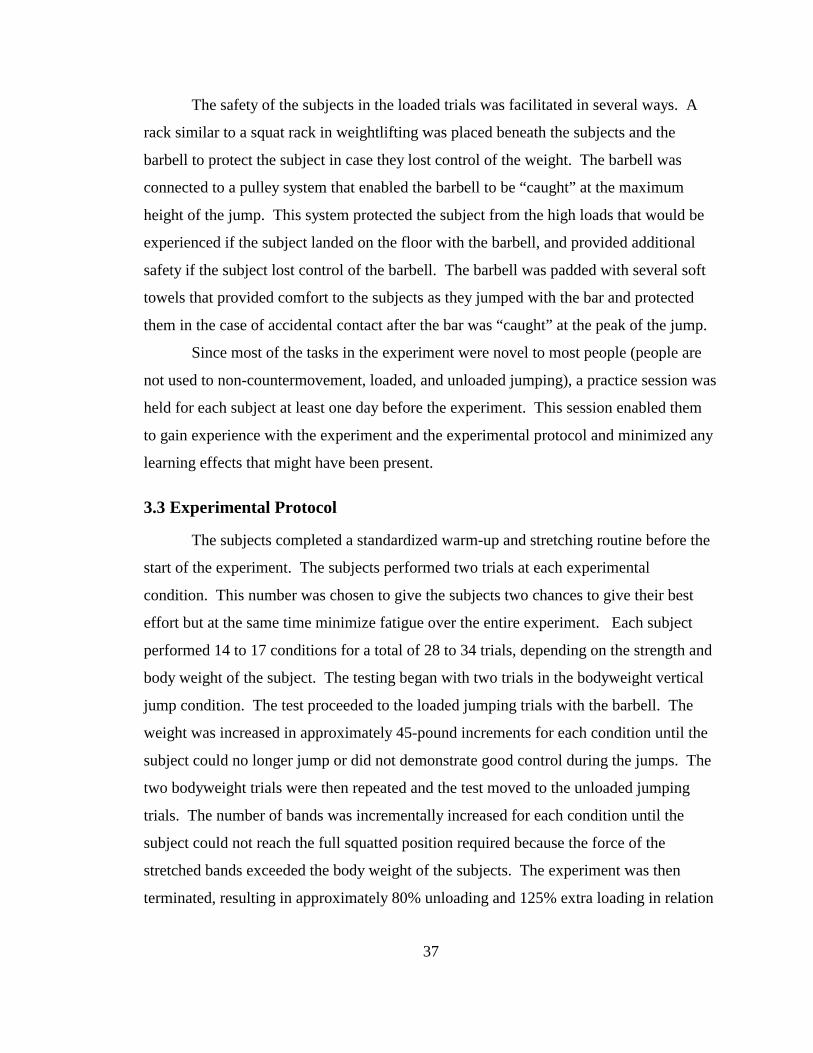
37
The safety of the subjects in the loaded trials was facilitated in several ways. A
rack similar to a squat rack in weightlifting was placed beneath the subjects and the
barbell to protect the subject in case they lost control of the weight. The barbell was
connected to a pulley system that enabled the barbell to be “caught” at the maximum
height of the jump. This system protected the subject from the high loads that would be
experienced if the subject landed on the floor with the barbell, and provided additional
safety if the subject lost control of the barbell. The barbell was padded with several soft
towels that provided comfort to the subjects as they jumped with the bar and protected
them in the case of accidental contact after the bar was “caught” at the peak of the jump.
Since most of the tasks in the experiment were novel to most people (people are
not used to non-countermovement, loaded, and unloaded jumping), a practice session was
held for each subject at least one day before the experiment. This session enabled them
to gain experience with the experiment and the experimental protocol and minimized any
learning effects that might have been present.
3.3 Experimental Protocol
The subjects completed a standardized warm-up and stretching routine before the
start of the experiment. The subjects performed two trials at each experimental
condition. This number was chosen to give the subjects two chances to give their best
effort but at the same time minimize fatigue over the entire experiment. Each subject
performed 14 to 17 conditions for a total of 28 to 34 trials, depending on the strength and
body weight of the subject. The testing began with two trials in the bodyweight vertical
jump condition. The test proceeded to the loaded jumping trials with the barbell. The
weight was increased in approximately 45-pound increments for each condition until the
subject could no longer jump or did not demonstrate good control during the jumps. The
two bodyweight trials were then repeated and the test moved to the unloaded jumping
trials. The number of bands was incrementally increased for each condition until the
subject could not reach the full squatted position required because the force of the
stretched bands exceeded the body weight of the subjects. The experiment was then
terminated, resulting in approximately 80% unloading and 125% extra loading in relation
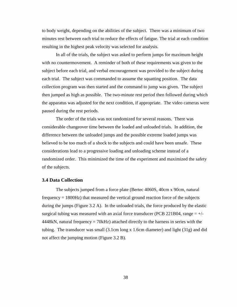
38
to body weight, depending on the abilities of the subject. There was a minimum of two
minutes rest between each trial to reduce the effects of fatigue. The trial at each condition
resulting in the highest peak velocity was selected for analysis.
In all of the trials, the subject was asked to perform jumps for maximum height
with no countermovement. A reminder of both of these requirements was given to the
subject before each trial, and verbal encouragement was provided to the subject during
each trial. The subject was commanded to assume the squatting position. The data
collection program was then started and the command to jump was given. The subject
then jumped as high as possible. The two-minute rest period then followed during which
the apparatus was adjusted for the next condition, if appropriate. The video cameras were
paused during the rest periods.
The order of the trials was not randomized for several reasons. There was
considerable changeover time between the loaded and unloaded trials. In addition, the
difference between the unloaded jumps and the possible extreme loaded jumps was
believed to be too much of a shock to the subjects and could have been unsafe. These
considerations lead to a progressive loading and unloading scheme instead of a
randomized order. This minimized the time of the experiment and maximized the safety
of the subjects.
3.4 Data Collection
The subjects jumped from a force plate (Bertec 4060S, 40cm x 90cm, natural
frequency = 1800Hz) that measured the vertical ground reaction force of the subjects
during the jumps (Figure 3.2 A). In the unloaded trials, the force produced by the elastic
surgical tubing was measured with an axial force transducer (PCB 221B04, range = +/-
4448kN, natural frequency = 70kHz) attached directly to the harness in series with the
tubing. The transducer was small (3.1cm long x 1.6cm diameter) and light (31g) and did
not affect the jumping motion (Figure 3.2 B).
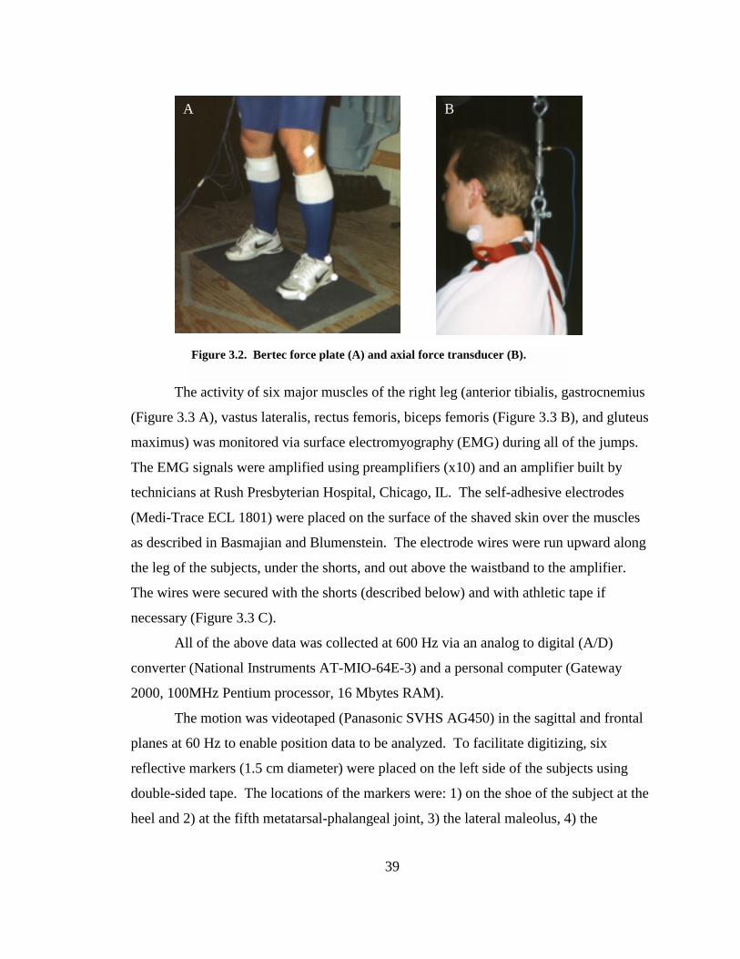
39
The activity of six major muscles of the right leg (anterior tibialis, gastrocnemius
(Figure 3.3 A), vastus lateralis, rectus femoris, biceps femoris (Figure 3.3 B), and gluteus
maximus) was monitored via surface electromyography (EMG) during all of the jumps.
The EMG signals were amplified using preamplifiers (x10) and an amplifier built by
technicians at Rush Presbyterian Hospital, Chicago, IL. The self-adhesive electrodes
(Medi-Trace ECL 1801) were placed on the surface of the shaved skin over the muscles
as described in Basmajian and Blumenstein. The electrode wires were run upward along
the leg of the subjects, under the shorts, and out above the waistband to the amplifier.
The wires were secured with the shorts (described below) and with athletic tape if
necessary (Figure 3.3 C).
All of the above data was collected at 600 Hz via an analog to digital (A/D)
converter (National Instruments AT-MIO-64E-3) and a personal computer (Gateway
2000, 100MHz Pentium processor, 16 Mbytes RAM).
The motion was videotaped (Panasonic SVHS AG450) in the sagittal and frontal
planes at 60 Hz to enable position data to be analyzed. To facilitate digitizing, six
reflective markers (1.5 cm diameter) were placed on the left side of the subjects using
double-sided tape. The locations of the markers were: 1) on the shoe of the subject at the
heel and 2) at the fifth metatarsal-phalangeal joint, 3) the lateral maleolus, 4) the
Figure 3.2. Bertec force plate (A) and axial force transducer (B).
A B
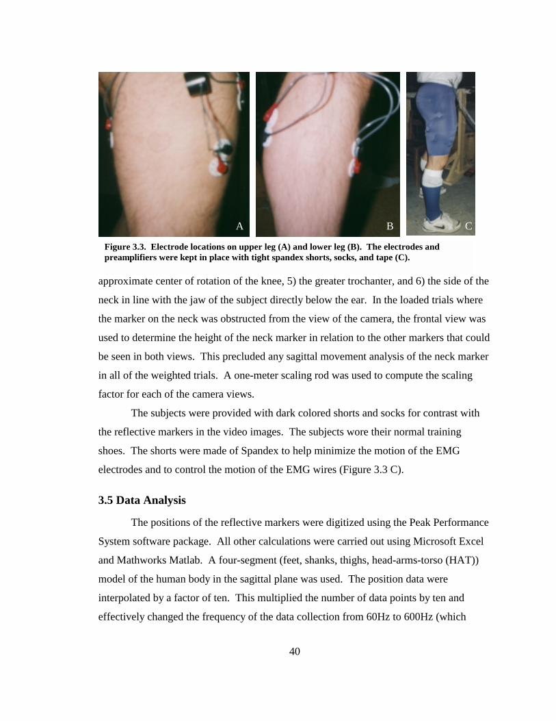
40
approximate center of rotation of the knee, 5) the greater trochanter, and 6) the side of the
neck in line with the jaw of the subject directly below the ear. In the loaded trials where
the marker on the neck was obstructed from the view of the camera, the frontal view was
used to determine the height of the neck marker in relation to the other markers that could
be seen in both views. This precluded any sagittal movement analysis of the neck marker
in all of the weighted trials. A one-meter scaling rod was used to compute the scaling
factor for each of the camera views.
The subjects were provided with dark colored shorts and socks for contrast with
the reflective markers in the video images. The subjects wore their normal training
shoes. The shorts were made of Spandex to help minimize the motion of the EMG
electrodes and to control the motion of the EMG wires (Figure 3.3 C).
3.5 Data Analysis
The positions of the reflective markers were digitized using the Peak Performance
System software package. All other calculations were carried out using Microsoft Excel
and Mathworks Matlab. A four-segment (feet, shanks, thighs, head-arms-torso (HAT))
model of the human body in the sagittal plane was used. The position data were
interpolated by a factor of ten. This multiplied the number of data points by ten and
effectively changed the frequency of the data collection from 60Hz to 600Hz (which
Figure 3.3. Electrode locations on upper leg (A) and lower leg (B). The electrodes and preamplifiers were kept in place with tight spandex shorts, socks, and tape (C).
A B C
41
matches the rest of the data and makes data analysis easier). This interpolation did not
increase the accuracy or change the values of any of the original calculated variables.
The video data was filtered with a fifth order Butterworth filter. The filtering frequency
was determined by filtering the data from one to 20Hz, computing the center of mass
velocity curve (see below), and comparing the velocity curve with the corresponding
center of mass velocity curve calculated with force plate data (see below). A least
squares difference approach was used to choose the best filtering frequency.
The velocity and acceleration of each of the markers was computed by
numerically differentiating the position data. In most of the loaded trials, the neck
marker was obstructed from the view of the sagittal camera by the barbell plates. To
construct the segment model the vertical position of the neck marker from the front view
was combined with the vertical positions of the other markers in the sagittal view. This
technique enabled vertical motion to be analyzed (which was most important for this
study), but horizontal motion for the HAT segment could not be analyzed.
The positions of the centers of mass of each of the segments and of the whole
body were computed using the body mass parameters of Zatsiorsky, et al. (1990). The
position of the center of mass of the HAT was adjusted to take into account the position
of the arms, which were raised to hold on to the barbell or wooden rod as described
above. The vertical velocities and accelerations of these points and the center of mass
were calculated by numerical differentiation of the position data.
In the bodyweight vertical jump and loaded jump trials, the governing equation is:
GRF - W = ma, (1)
where GRF is the vertical ground reaction force measured from the force plate, W is the
weight of the subject and the barbell combined, m is the mass of the subject and the
barbell, and a is the acceleration of the center of mass of the system. In the unloaded
trials, the governing equation is:
GRF - W + Fb = ma, (2)
where GRF, W, m, and a are as above, and Fb is the force provided by the elastic bands.
Using these equations, vertical ground reaction force was computed.
42
The vertical ground reaction force as measured from the force plate was also used
to calculate the velocity of the center of mass. The above equations, when solved for
acceleration and numerically integrated to estimate the area under the acceleration curve,
allowed the vertical velocity of the center of mass to be computed at each instant of time.
Vertical center of mass velocity and vertical ground reaction force were simply called
center of mass velocity and ground reaction force in this paper.
The angular velocity of the knee joint was calculated by numerically
differentiating the joint angle at each instant in time as determined from the video
analysis. An additional measure of leg extension velocity was computed by computing
the linear velocity between the hip and the ankle using the video data. This was a
technique that has not been seen in the force-velocity literature and was called leg
extension velocity in this paper.
The torque produced at the knee joint was computed using an inverse dynamics
approach (Winter, 1990) combining the data from the force plate, video, and body
segment parameter assumptions (Zatsiorsky, et al., (1990). The ground reaction force
data and the movement data of the foot were combined to calculate the resulting torque at
the ankle. This data was then used to calculate the torque produced at the knee.
Power was calculated in both the video method and the force plate method by
multiplying the corresponding ground reaction force by the velocity of the center of mass
at each instant in time. Power calculated in this way has sometimes been called ‘pseudo-
power’ because, strictly speaking, the ground reaction force does not act directly on the
center of mass, but it is quantitatively equal to the effective force that is acting at the
center of mass. However, it is also a common practice in the literature to refer to pseudo-
power as simply power; this paper will follow that practice as well. Power at the knee
joint was calculated by multiplying the corresponding torque by the angular velocity at
each moment in time. Another measure of power was attempted by multiplying leg
extension velocity by the corresponding ground reaction force. This has not been seen
before in the literature.
When necessary, the data from the force plate and the video analyses were
synchronized using the instant of takeoff as a reference. This moment in time was easily
43
determined from the ground reaction force-time curve as the point where there is zero
force. The moment of takeoff was also easily observed in the video analysis. The ratio
of recording speeds between the video and the other equipment was 1/10 producing
minimal error when the two sets of data were synchronized.
The data for each of the subjects was normalized so that the results from all of the
subjects could be combined and compared. The external load was normalized by
dividing the load at each condition by the body weight of the subject. Thus, the
normalized load in the body weight conditions was zero and the rest of the normalized
loads were fractions of body weight. Since the load was not constant in the unloaded
conditions, the load during the static squat before the jump was used for these plots. All
force, velocity, power, and time variables, regardless of the calculation procedure, were
normalized by dividing by the average body weight values of each parameter. Thus, all
of the normalized variables at the zero-load condition were equal to one.
Originally, EMG was to be analyzed in detail to determine the coordination
patterns of the vertical jumps under the various loading conditions. This proved to be
beyond the reasonable scope of the project, therefore only a few examples of EMG plots
were created for several loading conditions. This was accomplished by rectifying the
EMG signal and subjecting it to a low pass filter (same as above, 20 Hz), thereby
producing an EMG-envelope showing the major activation patterns of each muscle.
3.6 Parameter Combinations
One of the purposes of this study was to determine the best way to present force-
velocity and power-velocity relationships for multi-joint movements since there was an
unlimited number of choices for combinations of variables. Therefore, several
combinations were chosen to highlight combinations with high correlations and to
eliminate some of the possible combinations with low correlations. All of the following
combinations described were parametric relationships, i.e. one instant in time during each
condition was chosen and the values for each experimental variable, i.e. force, velocity,
or power, were determined at this instant; the individual points from each condition were
then combined in one ‘parametric’ plot.
44
The efficacy of the methods and protocols was investigated by examining the
center of mass velocity and ground reaction force-time relationships. The reactions of
each of the key variables in the study were examined in relation to the external load, the
only independent variable in this study. These key variables, maximum velocity of the
center of mass, the corresponding ground reaction force, maximum knee angular velocity,
maximum leg extension velocity, and the corresponding knee moment, were all plotted
against the external load. Total movement time from the onset of the movement to
takeoff, the time from initial movement to maximum center of mass velocity, and the
time from the maximum center of mass velocity to takeoff were investigated as a function
of load.
The instant when maximum velocity occurred during each jump was chosen as
the moment in time to analyze the force-velocity and power-velocity relationships in this
study. As discussed in the literature review, this selection is somewhat arbitrary. The
time of maximum velocity was chosen because it was easily identifiable, and it was
consistent with other force-velocity studies in the literature (see Tables 2.2-2.5). The
maximum center of mass velocity also corresponds to an instant in time where the
acceleration is zero. Analyzing force-velocity properties at this instant may make this
multi-joint study more comparable to single joint and/or muscle/fiber studies in the
literature that had constant velocity (zero acceleration) as a constraint. The instant of
time for maximum velocity was different for each type of analysis for a given jump,
depending on the velocity that was being measured. For example, the instant when
maximum velocity of the center of mass occurred was not the same as when the
maximum leg extension velocity or maximum knee angular velocity occurred.
The relationship between the maximum velocity of the center of mass of each
jump from the force plate and video analyses as well as the maximum leg extension
velocity and maximum knee angular velocity was investigated by plotting these terms
against their corresponding ground reaction forces. Maximum ground reaction force was
also studied briefly in relation to maximum center of mass velocity and to the center of
mass velocity that corresponded to the instant of maximum ground reaction force. Knee
moment was plotted as a function of maximum knee angular velocity and of maximum
45
leg extension velocity. Other than those involving leg extension velocity, these were all
common variable combinations that have been investigated in the literature (see Tables
2.4 and 2.5).
Power was investigated in several ways in this study. Power, in a force-velocity
context, is simply another way of presenting the data that may have additional meanings
in alternate contexts, i.e. athletic events. The first group of power curves used power
calculated by multiplying maximum center of mass velocity by its corresponding ground
reaction force. The relationship between power and load, which potentially has relevance
in weight training theory, was investigated by plotting the power corresponding to the
instant of maximum center of mass velocity against the corresponding external load. The
relationship between power and ground reaction force corresponding to the instant of
maximum center of mass velocity was also studied. Power corresponding to the instant
of maximum center of mass velocity and maximum center of mass velocity were plotted
together, as were corresponding power and maximum knee angular velocity, and
corresponding power and maximum leg extension velocity.
Knee angular velocity multiplied by maximum knee torque was used to calculate
knee power in the second group of power curves. Corresponding knee power calculated
in this way was plotted against maximum knee angular velocity and maximum leg
extension velocity. The third method for calculating power has not been seen in the
literature. This power measure was accomplished by multiplying the ground reaction
force by the maximum leg extension velocity and was presented by plotting it against the
maximum leg extension velocity and the external load.
3.7 Statistics
The force vs. velocity, force vs. load and velocity vs. load curves mentioned
above were fitted with two models: a second order polynomial using a least-squared
difference approach (except the ground reaction force vs. load relationship, which was fit
with a first order curve) and a hyperbolic model (Hill’s curve) using Newton’s Method
and the method of least squares to determine the constants. The power curves were fit
with the polynomial only. The second order polynomial was chosen because it was
46
simple, seemed to describe the force-velocity data well, and in the case of the power
curves, the theoretical model for power is a parabola which is a second order curve.
A measure of goodness of fit was determined for each relevant curve by
performing an intra-class correlation (Fleiss, 1986) between the data and the fitted
predictions. This correlation was a test of the relative homogeneity between the data and
the fit. Intra-class correlation reflects systematic differences in the data sets that a more
common measure such as Pearson’s product moment correlation would miss which
makes the former a better measure of fit. These models were then compared to each
other and the relevant literature. The polynomial and hyperbolic fits were not compared
statistically because there is no statistical meaning to comparing the shape of the curves.
The parabolic fit was either favorably or unfavorably compared to the Hill model with the
criteria described previously.
Since data from both the force plate method and the video method were used in
combination for some of the analyses, it was important to determine that the two methods
produced similar results. To that end, the maximum velocity of the center of mass,
corresponding ground reaction force, and load relationships were compared by
correlating the curve fits from each variable combination using the intra-class correlation
technique.
3.8 Delimitations of the Study
No matter how much effort is expended in the effort to control every aspect of a
scientific experiment, there are always weaknesses in the study. This experiment was no
exception. The main weakness of this study was the fact that body position could not be
controlled throughout the entire movement. This led to many questions as the data was
analyzed as reflected in the Discussion. However, this is an intrinsic problem found in
nearly all multi-joint investigations of any type.
Another problem was the fact that the barbell weights prevented the saggital
camera from picking up the neck marker. This meant that no analysis of the hip joint was
possible for the loaded conditions. There was a plan in place to digitize the end of the
barbell and to transpose that data to the position of the neck, but that method proved to be
47
impractical if not impossible with the data available. The vertical position of the neck
marker was measured from the front view and used as described earlier in this chapter.
The starting position of the subjects was not strictly controlled. The subjects were
instructed to start in a thighs horizontal position. The feet were not able to be placed flat
on the force plate in the unloaded conditions, so the subjects were instructed to begin
with the heels off of the ground in all of the conditions. Differences in ankle position
may have affected the initial length of the gastrocnemius, which could have affects at
both the ankle and the knee since it is a two-joint muscle. There was also the possibility
of a countermovement at the ankle, which may have been too small to be picked up by
the force plate. These factors can adversely affect several of the calculations if there are
large differences between trials and/or between subjects. Visual checks and verbal
encouragement were used to assist the subjects in assuming their starting position, and
the subjects were all required to attend a practice session before performing the
experiments. It is believed that this is not a serious problem.
Another potential delimitation was the fact that the subject population was more
diverse than originally hoped due to problems in the recruitment process. However, all of
the subjects were good athletes and had similar strength training regimes. Most of the
major differences between the subjects seemed to be greatly reduced with the simple
normalization techniques described in this chapter.
The elastic bands did not provide a constant unloading force on the subjects
throughout the entire movement. Using short bands stretched over a long distance
minimized this problem but it was impossible to eliminate completely. Many solutions
for unloading were discussed before the experiment, and this procedure was deemed to be
the best overall (see Appendix for pilot studies on alternate solutions). The non-constant
force issue was addressed by continuously measuring the force of the bands during the
movement with a force transducer and including this measurement in the calculations.
This was not done in other studies that used a similar protocol (Tsarouchas and
Klissouras, 1981).
The length of time that the entire experimental protocol took to perform for each
subject could have been a possible source of fatigue, which could preclude the subjects
48
from producing maximal efforts. This was addressed by giving the subjects at least two
minutes rest between trials and by accomplishing the more difficult loaded trials first
when the subjects were fresher. None of the subjects complained of fatigue when asked
during the experiment.
Because of fatigue, mechanical, and safety issues the order of the trials was not
randomized. Randomizing is always desirable in experimental procedures because it
reduced the chances that the performance order itself influences the results. As
mentioned in this chapter, the above issues outweighed the experimental concerns. There
is no way to know for sure that the order of the trials did not influence the outcome of the
experiment.
There is no way to determine that the subjects actually performed with maximum
effort. They were reminded of this requirement before each trial and were verbally
encouraged during the trials.
Most of the potential delimitations in this project were anticipated and
compensated for in the experimental protocol or in the analysis. It is believed that the
problems in this study are minimal and that the results seen in the next chapter are the
true reflection of the biomechanics of the vertical jump during loaded and unloaded
conditions.

49
Chapter 4 Results
50
The main purpose of this chapter is to present the results of the experiments
described in the Methods. The first section verifies the effectiveness of the experimental
apparatus and protocol and reveals some basic relationships between many of the
variables to be used in the following sections and the loading level. The next section
explores some of the possible variable combinations for force and velocity, and the
consistency of the results between subjects will be discussed. After that, the two main
measuring techniques for collecting force-velocity data will be compared. The fourth
section will compare the results to Hill’s curve for force-velocity. Finally, power
generated during the takeoffs will be discussed in relation to load, force and velocity.
Unless stated otherwise, all of the plots include data for all of the subjects from all of the
loading conditions.
4.1 Results of Individual Variables with Changes in Load
This section verified that the methods and protocol used in this experiment were
effective in producing a wide range in the main variables by showing how these variables
varied with changes in loading condition. These variables were: 1) center of mass
velocity, 2) ground reaction force, 3) knee angular velocity, 4) leg extension velocity, and
5) knee torque. Load was varied from approximately 80% of bodyweight unloading to
approximately 125% of bodyweight additional loading during the series of
noncountermovement jumps. The desired outcome was to produce as wide of a range of
forces, velocities, and torques as possible.
The loading had a predictable effect on the jumping performances of the subjects.
Figure 4.1 (A) shows how the velocity of the center of mass varied for one subject with
changes in external load. A general effect of increasing the load was to increase the total
time of the movement, i.e. the time from the onset of movement to the instant when the
feet lost contact with the ground (Figure 4.1 B). As shown by Figure 4.1 (C), the time
from the onset of the movement to the achievement of maximum velocity increased as
the external load increased. The time between the instant of maximum velocity and the
instant when the feet lost contact with the ground increased slightly with increased load
(Figure 4.1 D).
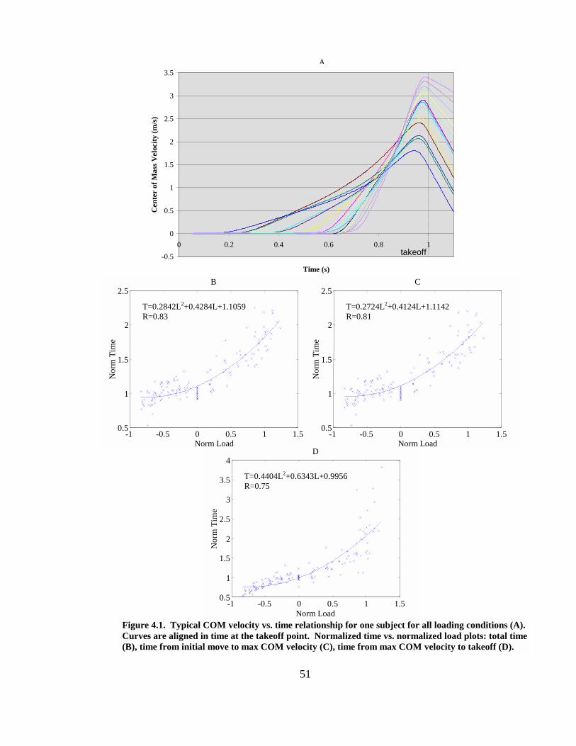
51
-1 -0.5 0 0.5 1 1.5 0.5
1
1.5
2
2.5
3
3.5
4 D
Norm Load
Nor
m T
ime
-1 -0.5 0 0.5 1 1.50.5
1
1.5
2
2.5 B
Norm Load
Nor
m T
ime
T=0.2842L2+0.4284L+1.1059 R=0.83
-1 -0.5 0 0.5 1 1.50.5
1
1.5
2
2.5C
Norm Load
Nor
m T
ime
T=0.2724L2+0.4124L+1.1142 R=0.81
Figure 4.1. Typical COM velocity vs. time relationship for one subject for all loading conditions (A). Curves are aligned in time at the takeoff point. Normalized time vs. normalized load plots: total time(B), time from initial move to max COM velocity (C), time from max COM velocity to takeoff (D).
T=0.4404L2+0.6343L+0.9956 R=0.75
-0.5
0
0.5
1
1.5
2
2.5
3
3.5
0 0.2 0.4 0.6 0.8 1
Time (s)
Cen
ter
of M
ass V
eloc
ity (m
/s)
takeoff
A
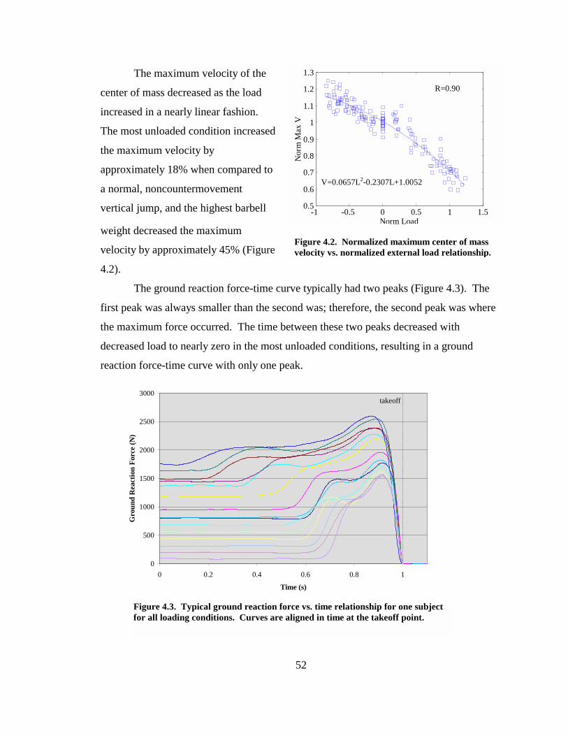
52
Figure 4.2. Normalized maximum center of mass velocity vs. normalized external load relationship.
-1 -0.5 0 0.5 1 1.50.5
0.6
0.7
0.8
0.9
1
1.1
1.2
1.3
Norm Load
Nor
m M
ax V
V=0.0657L2-0.2307L+1.0052
R=0.90
The maximum velocity of the
center of mass decreased as the load
increased in a nearly linear fashion.
The most unloaded condition increased
the maximum velocity by
approximately 18% when compared to
a normal, noncountermovement
vertical jump, and the highest barbell
weight decreased the maximum
velocity by approximately 45% (Figure
4.2).
The ground reaction force-time curve typically had two peaks (Figure 4.3). The
first peak was always smaller than the second was; therefore, the second peak was where
the maximum force occurred. The time between these two peaks decreased with
decreased load to nearly zero in the most unloaded conditions, resulting in a ground
reaction force-time curve with only one peak.
Figure 4.3. Typical ground reaction force vs. time relationship for one subject for all loading conditions. Curves are aligned in time at the takeoff point.
0
500
1000
1500
2000
2500
3000
0 0.2 0.4 0.6 0.8 1
Time (s)
Gro
und
Rea
ctio
n Fo
rce
(N)
takeoff
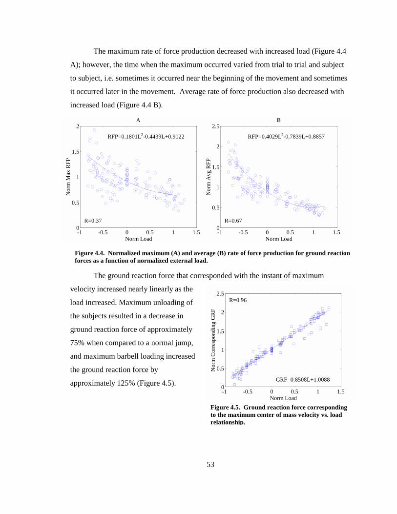
53
Figure 4.5. Ground reaction force corresponding to the maximum center of mass velocity vs. load relationship.
The maximum rate of force production decreased with increased load (Figure 4.4
A); however, the time when the maximum occurred varied from trial to trial and subject
to subject, i.e. sometimes it occurred near the beginning of the movement and sometimes
it occurred later in the movement. Average rate of force production also decreased with
increased load (Figure 4.4 B).
The ground reaction force that corresponded with the instant of maximum
velocity increased nearly linearly as the
load increased. Maximum unloading of
the subjects resulted in a decrease in
ground reaction force of approximately
75% when compared to a normal jump,
and maximum barbell loading increased
the ground reaction force by
approximately 125% (Figure 4.5).
Figure 4.4. Normalized maximum (A) and average (B) rate of force production for ground reaction forces as a function of normalized external load.
-1 -0.5 0 0.5 1 1.50
0.5
1
1.5
2 A
Norm Load
Nor
m M
ax R
FP
-1 -0.5 0 0.5 1 1.50
0.5
1
1.5
2
2.5B
Norm Load
Nor
m A
vg R
FP
RFP=0.1801L2-0.4439L+0.9122 RFP=0.4029L2-0.7839L+0.8857
R=0.37 R=0.67
-1 -0.5 0 0.5 1 1.50
0.5
1
1.5
2
2.5
Norm Load
Nor
m C
orre
spon
ding
GR
F
GRF=0.8508L+1.0088
R=0.96

54
The maximum knee angular velocity generally decreased as the load increased,
but the data were scattered (R=0.4942) and a specific trend was difficult to see (Figure
4.6 A). When fitted with a second-degree polynomial, individual subjects produced
relationships which were typically concave downward, but the shape of the curves were
only generally similar, ranging from a nearly linear decreasing line (Figure 4.6 B) to an
increasing-decreasing curved line (Figure 4.6 C).
Figure 4.6. Normalized maximum knee angular velocity vs. normalized load relationship (A). Maximum angular velocity vs. external load examples for two different subjects (B and C).
-800 -600 -400 -200 0 200 400 600 800 10009
1011
12
1314
1516
17
1819
B
Load (N)
Max
Ang
Kne
e V
(rad
/s)
R=0.83
-800 -600 -400 -200 0 200 400 600 800 10008
10
12
14
16
18
20
22C
Load (N)
Max
Ang
Kne
e V
(rad
/s)
R=0.43
-1 -0.5 0 0.5 1 1.50.4
0.6
0.8
1
1.2
1.4A
Norm Load
Nor
m M
ax K
nee
Ang
V
AngV=0.1774L2-0.1524L+0.941
R=0.49
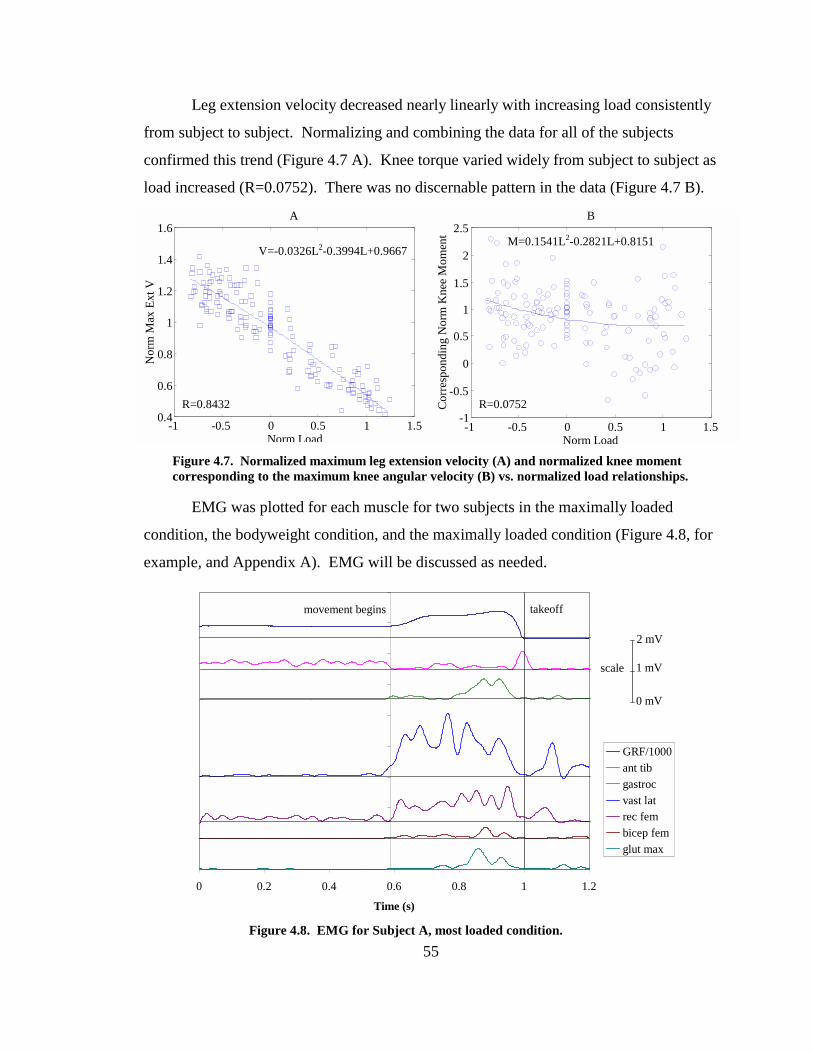
55
Leg extension velocity decreased nearly linearly with increasing load consistently
from subject to subject. Normalizing and combining the data for all of the subjects
confirmed this trend (Figure 4.7 A). Knee torque varied widely from subject to subject as
load increased (R=0.0752). There was no discernable pattern in the data (Figure 4.7 B).
EMG was plotted for each muscle for two subjects in the maximally loaded
condition, the bodyweight condition, and the maximally loaded condition (Figure 4.8, for
example, and Appendix A). EMG will be discussed as needed.
Figure 4.7. Normalized maximum leg extension velocity (A) and normalized knee moment corresponding to the maximum knee angular velocity (B) vs. normalized load relationships.
-1 -0.5 0 0.5 1 1.50.4
0.6
0.8
1
1.2
1.4
1.6 A
Norm Load
Nor
m M
ax E
xt V
-1 -0.5 0 0.5 1 1.5-1
-0.5
0
0.5
1
1.5
2
2.5B
Norm LoadC
orre
spon
ding
Nor
m K
nee
Mom
ent
V=-0.0326L2-0.3994L+0.9667M=0.1541L2-0.2821L+0.8151
R=0.8432 R=0.0752
Figure 4.8. EMG for Subject A, most loaded condition.
0 0.2 0.4 0.6 0.8 1 1.2
Time (s)
GRF/1000ant tibgastrocvast latrec fembicep femglut max
movement begins takeoff
2 mV
1 mV
0 mV
scale
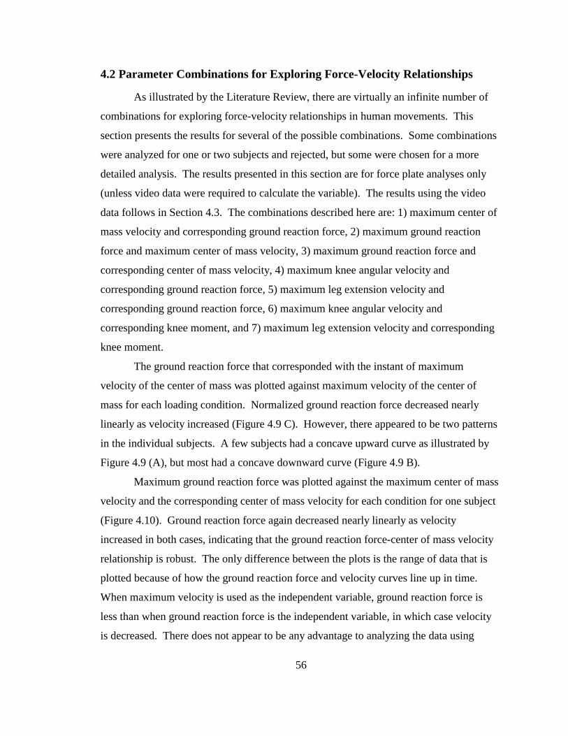
56
4.2 Parameter Combinations for Exploring Force-Velocity Relationships
As illustrated by the Literature Review, there are virtually an infinite number of
combinations for exploring force-velocity relationships in human movements. This
section presents the results for several of the possible combinations. Some combinations
were analyzed for one or two subjects and rejected, but some were chosen for a more
detailed analysis. The results presented in this section are for force plate analyses only
(unless video data were required to calculate the variable). The results using the video
data follows in Section 4.3. The combinations described here are: 1) maximum center of
mass velocity and corresponding ground reaction force, 2) maximum ground reaction
force and maximum center of mass velocity, 3) maximum ground reaction force and
corresponding center of mass velocity, 4) maximum knee angular velocity and
corresponding ground reaction force, 5) maximum leg extension velocity and
corresponding ground reaction force, 6) maximum knee angular velocity and
corresponding knee moment, and 7) maximum leg extension velocity and corresponding
knee moment.
The ground reaction force that corresponded with the instant of maximum
velocity of the center of mass was plotted against maximum velocity of the center of
mass for each loading condition. Normalized ground reaction force decreased nearly
linearly as velocity increased (Figure 4.9 C). However, there appeared to be two patterns
in the individual subjects. A few subjects had a concave upward curve as illustrated by
Figure 4.9 (A), but most had a concave downward curve (Figure 4.9 B).
Maximum ground reaction force was plotted against the maximum center of mass
velocity and the corresponding center of mass velocity for each condition for one subject
(Figure 4.10). Ground reaction force again decreased nearly linearly as velocity
increased in both cases, indicating that the ground reaction force-center of mass velocity
relationship is robust. The only difference between the plots is the range of data that is
plotted because of how the ground reaction force and velocity curves line up in time.
When maximum velocity is used as the independent variable, ground reaction force is
less than when ground reaction force is the independent variable, in which case velocity
is decreased. There does not appear to be any advantage to analyzing the data using
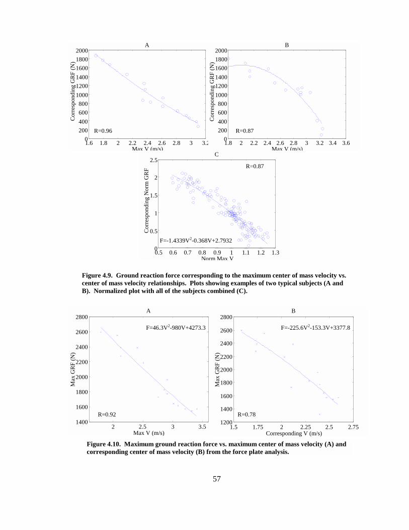
57
Figure 4.9. Ground reaction force corresponding to the maximum center of mass velocity vs. center of mass velocity relationships. Plots showing examples of two typical subjects (A and B). Normalized plot with all of the subjects combined (C).
2 2.5 3 3.51400
1600
1800
2000
2200
2400
2600
2800 A
Max V (m/s)
Max
GR
F (N
)
F=46.3V2-980V+4273.3
R=0.92
1.5 1.75 2 2.25 2.5 2.751200
1400
1600
1800
2000
2200
2400
2600
2800B
Corresponding V (m/s)
Max
GR
F (N
)
F=-225.6V2-153.3V+3377.8
R=0.78
Figure 4.10. Maximum ground reaction force vs. maximum center of mass velocity (A) and corresponding center of mass velocity (B) from the force plate analysis.
1.6 1.8 2 2.2 2.4 2.6 2.8 3 3.20 200 400 600 800
1000 1200 1400 1600 1800 2000
A
Max V (m/s)
Cor
resp
ondi
ng G
RF
(N)
1.8 2 2.2 2.4 2.6 2.8 3 3.2 3.4 3.60200400600800
100012001400160018002000
B
Max V (m/s)
Cor
resp
ondi
ng G
RF
(N)
0.5 0.6 0.7 0.8 0.9 1 1.1 1.2 1.30
0.5
1
1.5
2
2.5 C
Norm Max V
Cor
resp
ondi
ng N
orm
GR
F
F=-1.4339V2-0.368V+2.7932
R=0.96 R=0.87
R=0.87
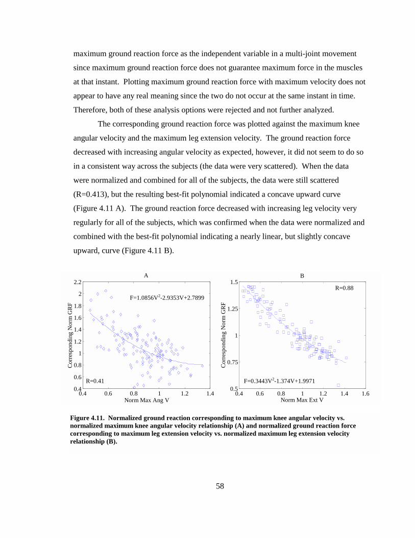
58
maximum ground reaction force as the independent variable in a multi-joint movement
since maximum ground reaction force does not guarantee maximum force in the muscles
at that instant. Plotting maximum ground reaction force with maximum velocity does not
appear to have any real meaning since the two do not occur at the same instant in time.
Therefore, both of these analysis options were rejected and not further analyzed.
The corresponding ground reaction force was plotted against the maximum knee
angular velocity and the maximum leg extension velocity. The ground reaction force
decreased with increasing angular velocity as expected, however, it did not seem to do so
in a consistent way across the subjects (the data were very scattered). When the data
were normalized and combined for all of the subjects, the data were still scattered
(R=0.413), but the resulting best-fit polynomial indicated a concave upward curve
(Figure 4.11 A). The ground reaction force decreased with increasing leg velocity very
regularly for all of the subjects, which was confirmed when the data were normalized and
combined with the best-fit polynomial indicating a nearly linear, but slightly concave
upward, curve (Figure 4.11 B).
Figure 4.11. Normalized ground reaction corresponding to maximum knee angular velocity vs. normalized maximum knee angular velocity relationship (A) and normalized ground reaction force corresponding to maximum leg extension velocity vs. normalized maximum leg extension velocity relationship (B).
0.4 0.6 0.8 1 1.2 1.40.4
0.6
0.8
1
1.2
1.4
1.6
1.8
2
2.2A
Norm Max Ang V
Cor
resp
ondi
ng N
orm
GR
F
F=1.0856V2-2.9353V+2.7899
R=0.41
0.4 0.6 0.8 1 1.2 1.4 1.60.5
0.75
1
1.25
1.5B
Norm Max Ext V
Cor
resp
ondi
ng N
orm
GR
F
F=0.3443V2-1.374V+1.9971
R=0.88
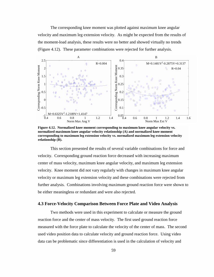
59
The corresponding knee moment was plotted against maximum knee angular
velocity and maximum leg extension velocity. As might be expected from the results of
the moment-load analysis, these results were no better and showed virtually no trends
(Figure 4.12). These parameter combinations were rejected for further analysis.
This section presented the results of several variable combinations for force and
velocity. Corresponding ground reaction force decreased with increasing maximum
center of mass velocity, maximum knee angular velocity, and maximum leg extension
velocity. Knee moment did not vary regularly with changes in maximum knee angular
velocity or maximum leg extension velocity and these combinations were rejected from
further analysis. Combinations involving maximum ground reaction force were shown to
be either meaningless or redundant and were also rejected.
4.3 Force-Velocity Comparison Between Force Plate and Video Analysis
Two methods were used in this experiment to calculate or measure the ground
reaction force and the center of mass velocity. The first used ground reaction force
measured with the force plate to calculate the velocity of the center of mass. The second
used video position data to calculate velocity and ground reaction force. Using video
data can be problematic since differentiation is used in the calculation of velocity and
Figure 4.12. Normalized knee moment corresponding to maximum knee angular velocity vs. normalized maximum knee angular velocity relationship (A) and normalized knee moment corresponding to maximum leg extension velocity vs. normalized maximum leg extension velocity relationship (B).
0.4 0.6 0.8 1 1.2 1.4-1
-0.5
0
0.5
1
1.5
2
2.5A
Norm Max Ang V
Cor
resp
ondi
ng N
orm
Kne
e M
omen
t
M=0.6325V2-1.2189V+1.4147
R=0.004
0.4 0.6 0.8 1 1.2 1.4 1.60.05
0.1
0.15
0.2
0.25
0.3
0.35
0.4B
Norm Max Ext V C
orre
spon
ding
Nor
m K
nee
Mom
ent M=0.1481V2-0.2875V+0.3137
R=0.04
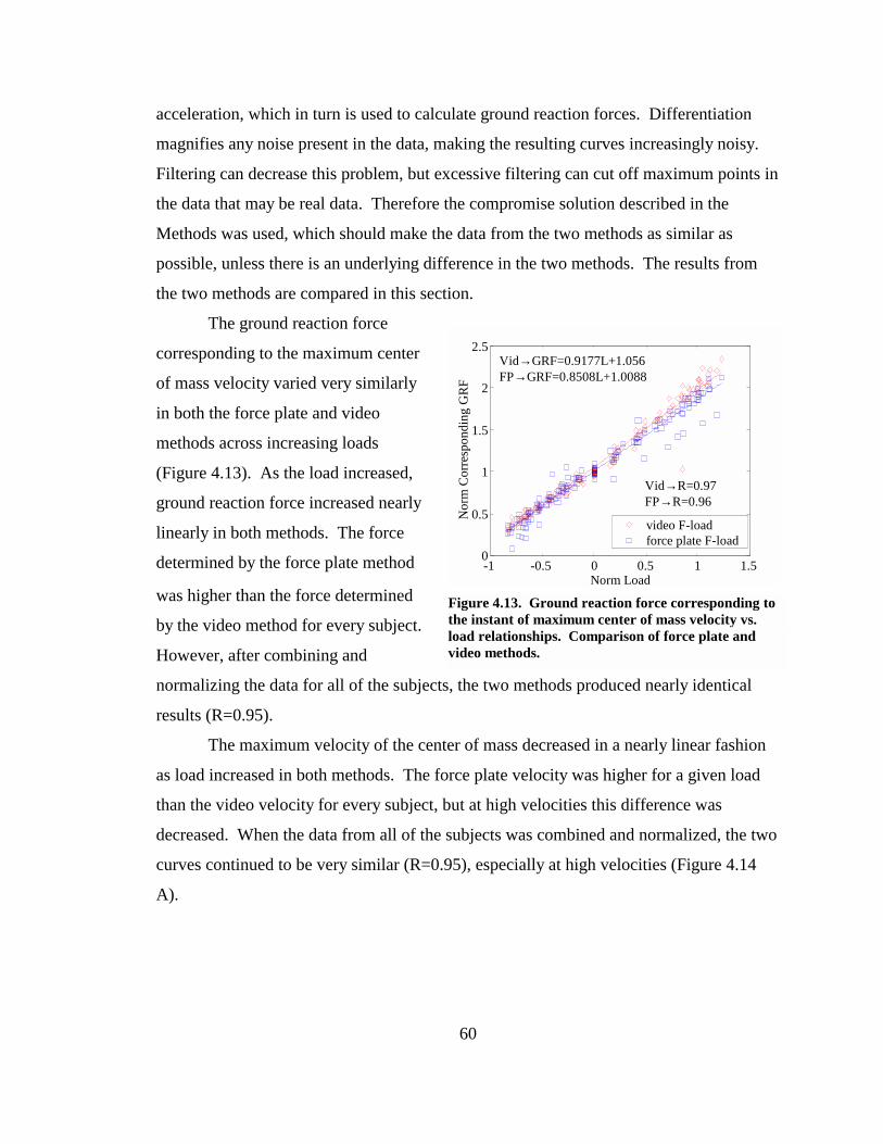
60
acceleration, which in turn is used to calculate ground reaction forces. Differentiation
magnifies any noise present in the data, making the resulting curves increasingly noisy.
Filtering can decrease this problem, but excessive filtering can cut off maximum points in
the data that may be real data. Therefore the compromise solution described in the
Methods was used, which should make the data from the two methods as similar as
possible, unless there is an underlying difference in the two methods. The results from
the two methods are compared in this section.
The ground reaction force
corresponding to the maximum center
of mass velocity varied very similarly
in both the force plate and video
methods across increasing loads
(Figure 4.13). As the load increased,
ground reaction force increased nearly
linearly in both methods. The force
determined by the force plate method
was higher than the force determined
by the video method for every subject.
However, after combining and
normalizing the data for all of the subjects, the two methods produced nearly identical
results (R=0.95).
The maximum velocity of the center of mass decreased in a nearly linear fashion
as load increased in both methods. The force plate velocity was higher for a given load
than the video velocity for every subject, but at high velocities this difference was
decreased. When the data from all of the subjects was combined and normalized, the two
curves continued to be very similar (R=0.95), especially at high velocities (Figure 4.14
A).
Figure 4.13. Ground reaction force corresponding to the instant of maximum center of mass velocity vs. load relationships. Comparison of force plate and video methods.
-1 -0.5 0 0.5 1 1.50
0.5
1
1.5
2
2.5
Norm Load
Nor
m C
orre
spon
ding
GR
F
video F-load force plate F-load
Vid→GRF=0.9177L+1.056 FP→GRF=0.8508L+1.0088
Vid→R=0.97 FP→R=0.96
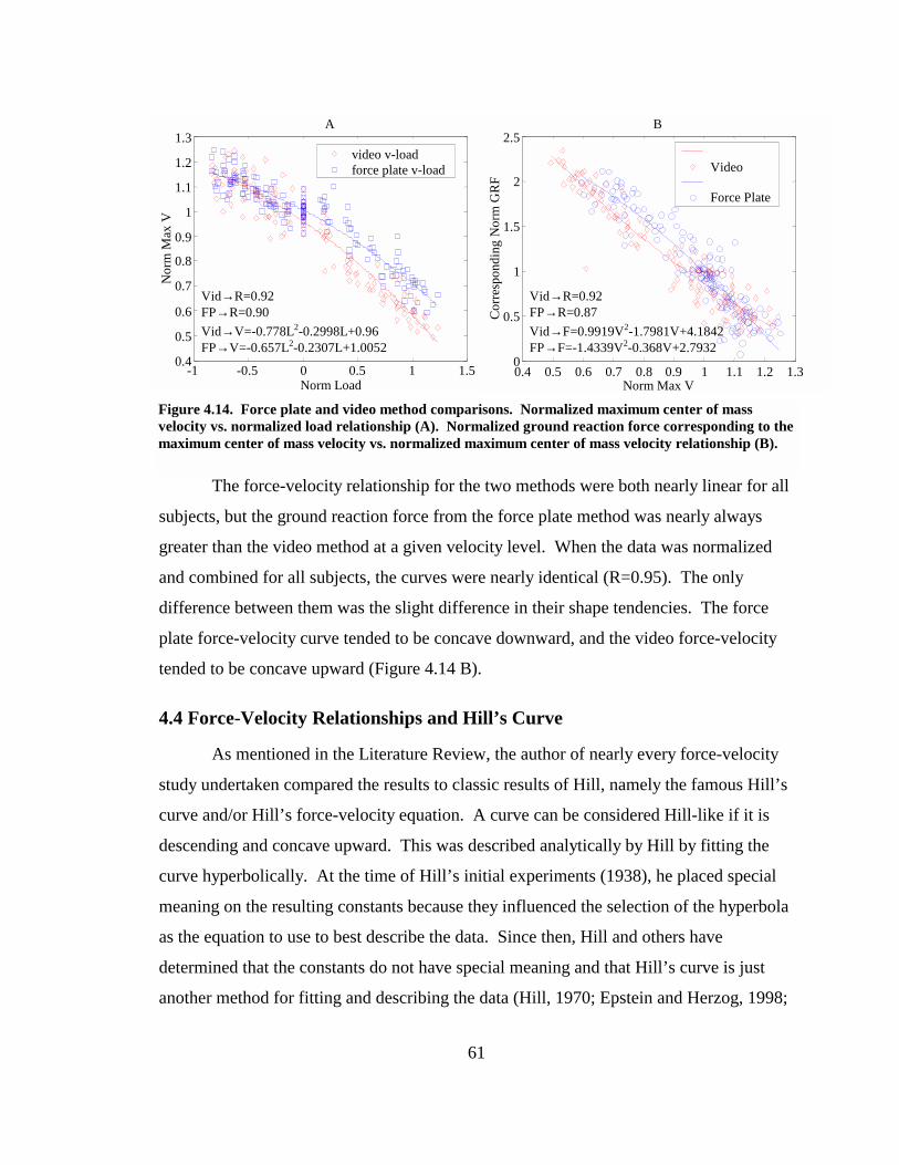
61
The force-velocity relationship for the two methods were both nearly linear for all
subjects, but the ground reaction force from the force plate method was nearly always
greater than the video method at a given velocity level. When the data was normalized
and combined for all subjects, the curves were nearly identical (R=0.95). The only
difference between them was the slight difference in their shape tendencies. The force
plate force-velocity curve tended to be concave downward, and the video force-velocity
tended to be concave upward (Figure 4.14 B).
4.4 Force-Velocity Relationships and Hill’s Curve
As mentioned in the Literature Review, the author of nearly every force-velocity
study undertaken compared the results to classic results of Hill, namely the famous Hill’s
curve and/or Hill’s force-velocity equation. A curve can be considered Hill-like if it is
descending and concave upward. This was described analytically by Hill by fitting the
curve hyperbolically. At the time of Hill’s initial experiments (1938), he placed special
meaning on the resulting constants because they influenced the selection of the hyperbola
as the equation to use to best describe the data. Since then, Hill and others have
determined that the constants do not have special meaning and that Hill’s curve is just
another method for fitting and describing the data (Hill, 1970; Epstein and Herzog, 1998;
Figure 4.14. Force plate and video method comparisons. Normalized maximum center of mass velocity vs. normalized load relationship (A). Normalized ground reaction force corresponding to the maximum center of mass velocity vs. normalized maximum center of mass velocity relationship (B).
-1 -0.5 0 0.5 1 1.50.4
0.5
0.6
0.7
0.8 0.9
1
1.1
1.2
1.3
Norm Load
Nor
m M
ax V
A
video v-load force plate v-load
0.4 0.5 0.6 0.7 0.8 0.9 1 1.1 1.2 1.30
0.5
1
1.5
2
2.5B
Norm Max V
Cor
resp
ondi
ng N
orm
GR
F
Video Force Plate
Vid→V=-0.778L2-0.2998L+0.96 FP→V=-0.657L2-0.2307L+1.0052
Vid→F=0.9919V2-1.7981V+4.1842 FP→F=-1.4339V2-0.368V+2.7932
Vid→R=0.92 FP→R=0.90
Vid→R=0.92 FP→R=0.87
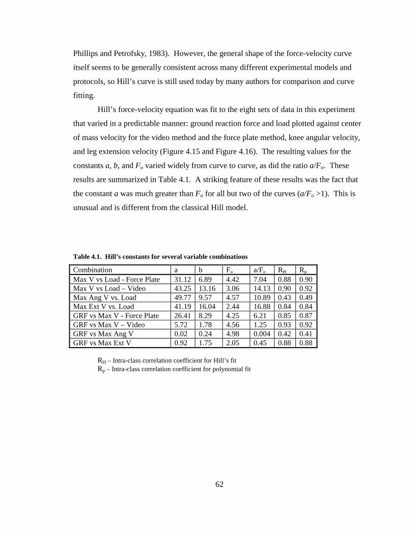
62
Phillips and Petrofsky, 1983). However, the general shape of the force-velocity curve
itself seems to be generally consistent across many different experimental models and
protocols, so Hill’s curve is still used today by many authors for comparison and curve
fitting.
Hill’s force-velocity equation was fit to the eight sets of data in this experiment
that varied in a predictable manner: ground reaction force and load plotted against center
of mass velocity for the video method and the force plate method, knee angular velocity,
and leg extension velocity (Figure 4.15 and Figure 4.16). The resulting values for the
constants a, b, and Fo varied widely from curve to curve, as did the ratio a/Fo. These
results are summarized in Table 4.1. A striking feature of these results was the fact that
the constant a was much greater than Fo for all but two of the curves (a/Fo >1). This is
unusual and is different from the classical Hill model.
Table 4.1. Hill’s constants for several variable combinations
Combination a b Fo a/Fo RH Rp Max V vs Load - Force Plate 31.12 6.89 4.42 7.04 0.88 0.90 Max V vs Load – Video 43.25 13.16 3.06 14.13 0.90 0.92 Max Ang V vs. Load 49.77 9.57 4.57 10.89 0.43 0.49 Max Ext V vs. Load 41.19 16.04 2.44 16.88 0.84 0.84 GRF vs Max V - Force Plate 26.41 8.29 4.25 6.21 0.85 0.87 GRF vs Max V – Video 5.72 1.78 4.56 1.25 0.93 0.92 GRF vs Max Ang V 0.02 0.24 4.98 0.004 0.42 0.41 GRF vs Max Ext V 0.92 1.75 2.05 0.45 0.88 0.88
RH – Intra-class correlation coefficient for Hill’s fit Rp – Intra-class correlation coefficient for polynomial fit

63
Figure 4.15. Hill fits for maximum center of mass velocity, force plate analysis (A), maximum center of mass velocity, video analysis (B), maximum knee angular velocity (C), and maximum leg extension velocity (D) vs. external load.
-1 -0.5 0 0.5 1 1.50.5
0.6
0.7
0.8
0.9
1
1.1
1.2
1.3A
Norm Load
Nor
m M
ax V
a=31.12 b=6.89 Fo=4.42 a/Fo=7.04
R=0.88
-1 -0.5 0 0.5 1 1.50.4
0.5
0.6
0.7
0.8
0.9
1
1.1
1.2
1.3B
Norm Load
Nor
m M
ax V
a=43.25 b=13.16 Fo=3.06 a/Fo=14.13
R=0.90
-1 -0.5 0 0.5 1 1.50.4
0.6
0.8
1
1.2
1.4C
Norm Load
Nor
m M
ax K
nee
Ang
a=49.77 b=9.57 Fo=4.57 a/Fo=10.89
R=0.43
-1 -0.5 0 0.5 1 1.50.4
0.6
0.8
1
1.2
1.4
1.6D
Norm Load
Nor
m M
ax E
xt V
a=41.19 b=16.04 Fo=2.44 a/Fo=16.88
R=0.84
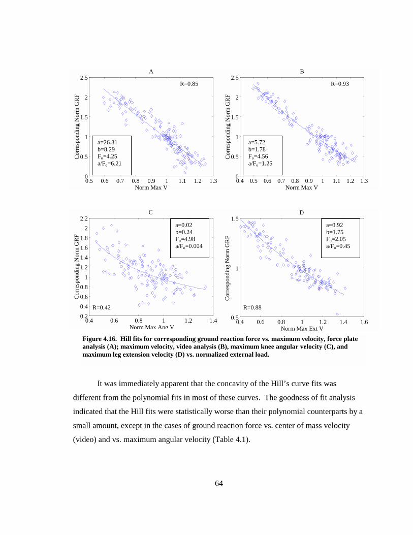
64
It was immediately apparent that the concavity of the Hill’s curve fits was
different from the polynomial fits in most of these curves. The goodness of fit analysis
indicated that the Hill fits were statistically worse than their polynomial counterparts by a
small amount, except in the cases of ground reaction force vs. center of mass velocity
(video) and vs. maximum angular velocity (Table 4.1).
Figure 4.16. Hill fits for corresponding ground reaction force vs. maximum velocity, force plate analysis (A); maximum velocity, video analysis (B), maximum knee angular velocity (C), and maximum leg extension velocity (D) vs. normalized external load.
0.4 0.6 0.8 1 1.2 1.40.20.40.60.8
11.21.41.61.8
22.2
C
Norm Max Ang V
Cor
resp
ondi
ng N
orm
GR
F
0.5 0.6 0.7 0.8 0.9 1 1.1 1.2 1.30
0.5
1
1.5
2
2.5A
Norm Max V
Cor
resp
ondi
ng N
orm
GR
F
a=26.31 b=8.29 Fo=4.25 a/Fo=6.21
R=0.85
0.4 0.5 0.6 0.7 0.8 0.9 1 1.1 1.2 1.30
0.5
1
1.5
2
2.5B
Norm Max V
Cor
resp
ondi
ng N
orm
GR
F
a=5.72 b=1.78 Fo=4.56 a/Fo=1.25
R=0.93
0.4 0.6 0.8 1 1.2 1.4 1.60.5
1
1.5D
Norm Max Ext V
Cor
resp
ondi
ng N
orm
GR
Fa=0.92 b=1.75 Fo=2.05 a/Fo=0.45
R=0.88
a=0.02 b=0.24 Fo=4.98 a/Fo=0.004
R=0.42
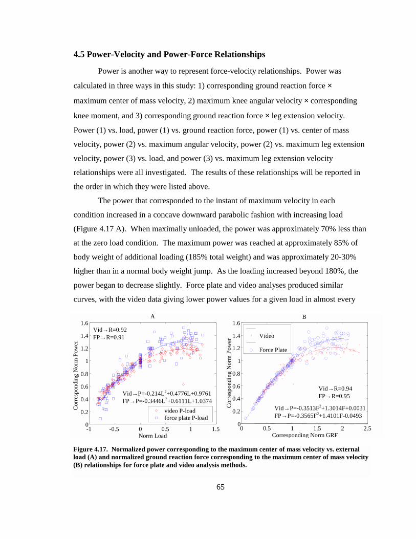
65
4.5 Power-Velocity and Power-Force Relationships
Power is another way to represent force-velocity relationships. Power was
calculated in three ways in this study: 1) corresponding ground reaction force ×
maximum center of mass velocity, 2) maximum knee angular velocity × corresponding
knee moment, and 3) corresponding ground reaction force × leg extension velocity.
Power (1) vs. load, power (1) vs. ground reaction force, power (1) vs. center of mass
velocity, power (2) vs. maximum angular velocity, power (2) vs. maximum leg extension
velocity, power (3) vs. load, and power (3) vs. maximum leg extension velocity
relationships were all investigated. The results of these relationships will be reported in
the order in which they were listed above.
The power that corresponded to the instant of maximum velocity in each
condition increased in a concave downward parabolic fashion with increasing load
(Figure 4.17 A). When maximally unloaded, the power was approximately 70% less than
at the zero load condition. The maximum power was reached at approximately 85% of
body weight of additional loading (185% total weight) and was approximately 20-30%
higher than in a normal body weight jump. As the loading increased beyond 180%, the
power began to decrease slightly. Force plate and video analyses produced similar
curves, with the video data giving lower power values for a given load in almost every
Figure 4.17. Normalized power corresponding to the maximum center of mass velocity vs. external load (A) and normalized ground reaction force corresponding to the maximum center of mass velocity (B) relationships for force plate and video analysis methods.
-1 -0.5 0 0.5 1 1.50
0.2
0.4
0.6
0.8
1
1.2
1.4
1.6
Norm Load
Cor
resp
ondi
ng N
orm
Pow
er
A
video P-loadforce plate P-load
Vid→P=-0.214L2+0.4776L+0.9761 FP→P=-0.3446L2+0.6111L+1.0374
0 0.5 1 1.5 2 2.50
0.2
0.4
0.6
0.8
1
1.2
1.4
1.6B
Corresponding Norm GRF
Cor
resp
ondi
ng N
orm
Pow
er
Video Force Plate
Vid→P=-0.3513F2+1.3014F+0.0031FP→P=-0.3565F2+1.4101F-0.0493
Vid→R=0.94 FP→R=0.95
Vid→R=0.92 FP→R=0.91
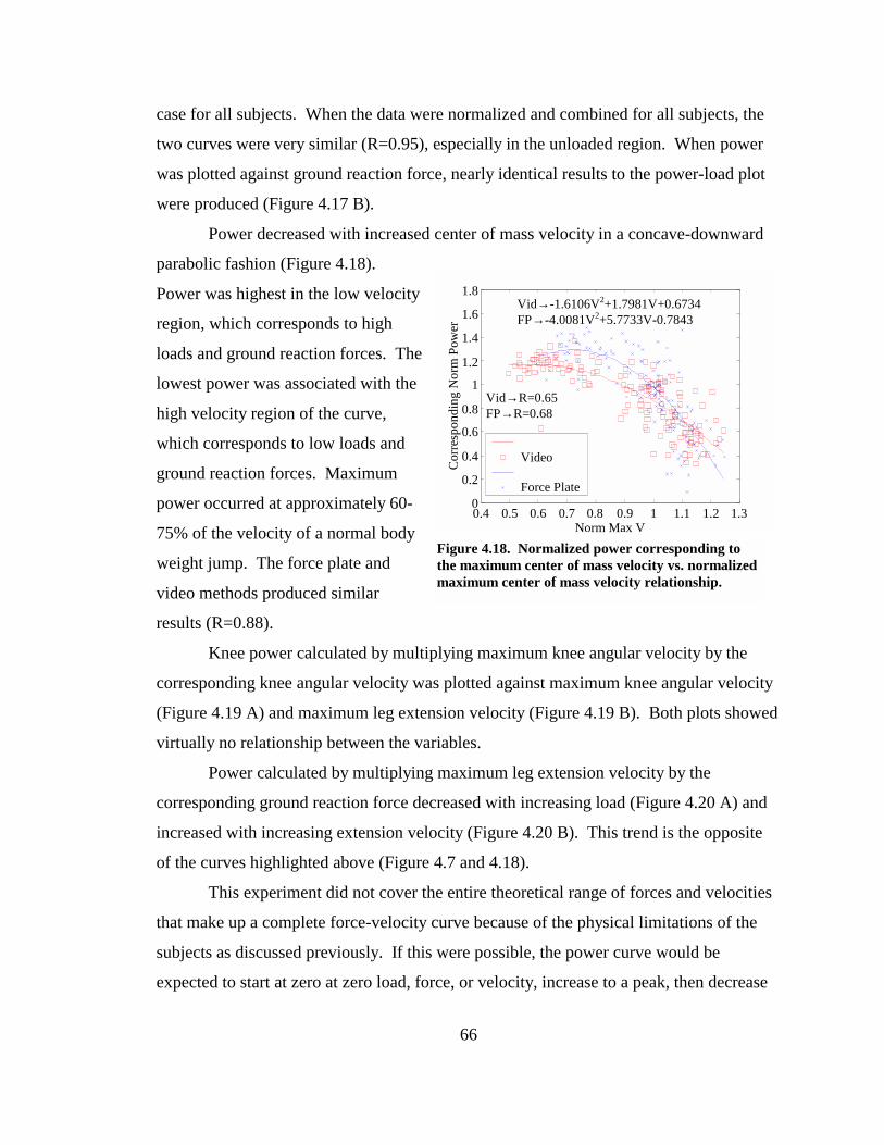
66
case for all subjects. When the data were normalized and combined for all subjects, the
two curves were very similar (R=0.95), especially in the unloaded region. When power
was plotted against ground reaction force, nearly identical results to the power-load plot
were produced (Figure 4.17 B).
Power decreased with increased center of mass velocity in a concave-downward
parabolic fashion (Figure 4.18).
Power was highest in the low velocity
region, which corresponds to high
loads and ground reaction forces. The
lowest power was associated with the
high velocity region of the curve,
which corresponds to low loads and
ground reaction forces. Maximum
power occurred at approximately 60-
75% of the velocity of a normal body
weight jump. The force plate and
video methods produced similar
results (R=0.88).
Knee power calculated by multiplying maximum knee angular velocity by the
corresponding knee angular velocity was plotted against maximum knee angular velocity
(Figure 4.19 A) and maximum leg extension velocity (Figure 4.19 B). Both plots showed
virtually no relationship between the variables.
Power calculated by multiplying maximum leg extension velocity by the
corresponding ground reaction force decreased with increasing load (Figure 4.20 A) and
increased with increasing extension velocity (Figure 4.20 B). This trend is the opposite
of the curves highlighted above (Figure 4.7 and 4.18).
This experiment did not cover the entire theoretical range of forces and velocities
that make up a complete force-velocity curve because of the physical limitations of the
subjects as discussed previously. If this were possible, the power curve would be
expected to start at zero at zero load, force, or velocity, increase to a peak, then decrease
Figure 4.18. Normalized power corresponding to the maximum center of mass velocity vs. normalized maximum center of mass velocity relationship.
0.4 0.5 0.6 0.7 0.8 0.9 1 1.1 1.2 1.30
0.2
0.4
0.6
0.8
1
1.2
1.4
1.6
1.8
Norm Max V
Cor
resp
ondi
ng N
orm
Pow
er
Video Force Plate
Vid→R=0.65 FP→R=0.68
Vid→-1.6106V2+1.7981V+0.6734 FP→-4.0081V2+5.7733V-0.7843
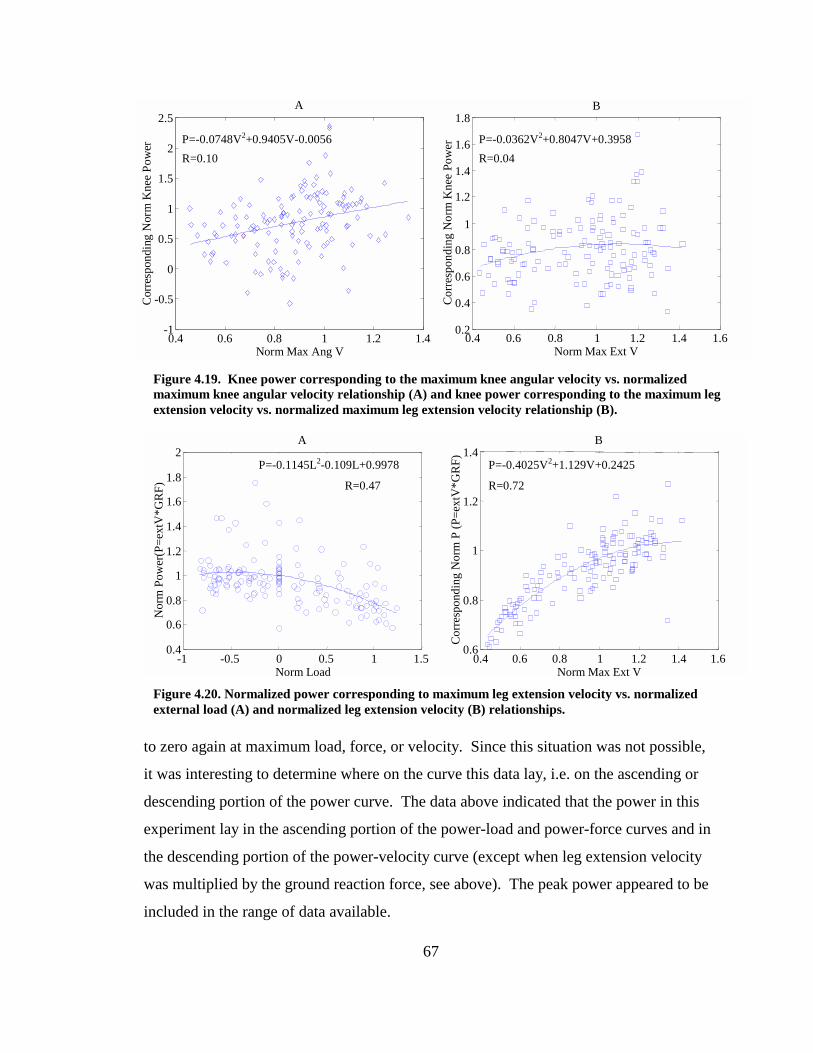
67
to zero again at maximum load, force, or velocity. Since this situation was not possible,
it was interesting to determine where on the curve this data lay, i.e. on the ascending or
descending portion of the power curve. The data above indicated that the power in this
experiment lay in the ascending portion of the power-load and power-force curves and in
the descending portion of the power-velocity curve (except when leg extension velocity
was multiplied by the ground reaction force, see above). The peak power appeared to be
included in the range of data available.
0.4 0.6 0.8 1 1.2 1.4-1
-0.5
0
0.5
1
1.5
2
2.5A
Norm Max Ang V
Cor
resp
ondi
ng N
orm
Kne
e Po
wer P=-0.0748V2+0.9405V-0.0056
R=0.10
0.4 0.6 0.8 1 1.2 1.4 1.60.2
0.4
0.6
0.8
1
1.2
1.4
1.6
1.8B
Norm Max Ext V
Cor
resp
ondi
ng N
orm
Kne
e Po
wer
P=-0.0362V2+0.8047V+0.3958 R=0.04
-1 -0.5 0 0.5 1 1.50.4
0.6
0.8
1
1.2
1.4
1.6
1.8
2 A
Norm Load
Nor
m P
ower
(P=e
xtV
*GR
F)
P=-0.1145L2-0.109L+0.9978
R=0.47
0.4 0.6 0.8 1 1.2 1.4 1.60.6
0.8
1
1.2
1.4B
Norm Max Ext V
Cor
resp
ondi
ng N
orm
P (P
=ext
V*G
RF)
P=-0.4025V2+1.129V+0.2425
R=0.72
Figure 4.19. Knee power corresponding to the maximum knee angular velocity vs. normalized maximum knee angular velocity relationship (A) and knee power corresponding to the maximum leg extension velocity vs. normalized maximum leg extension velocity relationship (B).
Figure 4.20. Normalized power corresponding to maximum leg extension velocity vs. normalized external load (A) and normalized leg extension velocity (B) relationships.

68
Chapter 5 Discussion
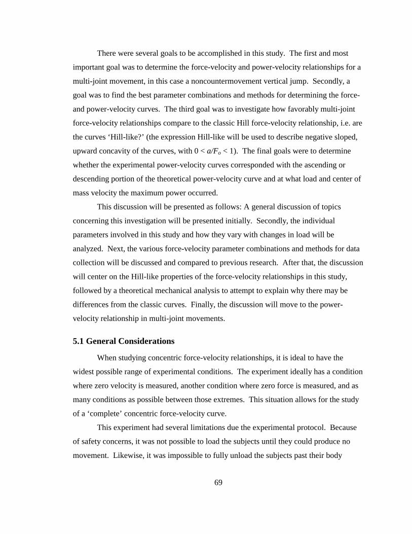
69
There were several goals to be accomplished in this study. The first and most
important goal was to determine the force-velocity and power-velocity relationships for a
multi-joint movement, in this case a noncountermovement vertical jump. Secondly, a
goal was to find the best parameter combinations and methods for determining the force-
and power-velocity curves. The third goal was to investigate how favorably multi-joint
force-velocity relationships compare to the classic Hill force-velocity relationship, i.e. are
the curves ‘Hill-like?’ (the expression Hill-like will be used to describe negative sloped,
upward concavity of the curves, with 0 < a/Fo < 1). The final goals were to determine
whether the experimental power-velocity curves corresponded with the ascending or
descending portion of the theoretical power-velocity curve and at what load and center of
mass velocity the maximum power occurred.
This discussion will be presented as follows: A general discussion of topics
concerning this investigation will be presented initially. Secondly, the individual
parameters involved in this study and how they vary with changes in load will be
analyzed. Next, the various force-velocity parameter combinations and methods for data
collection will be discussed and compared to previous research. After that, the discussion
will center on the Hill-like properties of the force-velocity relationships in this study,
followed by a theoretical mechanical analysis to attempt to explain why there may be
differences from the classic curves. Finally, the discussion will move to the power-
velocity relationship in multi-joint movements.
5.1 General Considerations
When studying concentric force-velocity relationships, it is ideal to have the
widest possible range of experimental conditions. The experiment ideally has a condition
where zero velocity is measured, another condition where zero force is measured, and as
many conditions as possible between those extremes. This situation allows for the study
of a ‘complete’ concentric force-velocity curve.
This experiment had several limitations due the experimental protocol. Because
of safety concerns, it was not possible to load the subjects until they could produce no
movement. Likewise, it was impossible to fully unload the subjects past their body
70
weight since they would have been suspended before the attempt and jumping would
have been impossible. The range of force and velocity data in this study is larger than in
any other published study, but the range is still only a part of the theoretical force-
velocity curve.
The height of the jumps across the experimental conditions seemed to change, as
might be expected. As the load was increased, the height of the jump decreased.
However, some of the perceived changes in jump height may have been artifacts of the
experimental protocol. The barbell in the loaded conditions was “caught” in mid flight to
add to the comfort and safety of the subjects upon landing. Therefore the subjects
became two separate masses during the flight phase and the subject landed with a
different mass than at takeoff. Similarly, the subjects in the unloaded conditions were
suspended from above with elastic tubing, which affected the natural flight of the
subjects. Therefore, no attempt was made to calculate the height of the jump or make any
evaluation of the flight time. Everything after the time of takeoff was ignored and was
not included in the discussion.
The choice of the maximum center of mass velocity as the time when most of the
variables were compared has some interesting ramifications. As mentioned briefly in the
Methods, the instant of maximum center of mass velocity corresponds to the instant when
the acceleration of the center of mass is zero. This means that the ground reaction force
is equal to the body weight and the additional load (or subtracted load in the unloaded
cases). This moment in time was chosen in part because many of the classical force-
velocity studies controlled the motion such that the acceleration was zero, perhaps
making the current study and the classical studies more comparable. However, the
classical studies ignored the mass of the muscle itself, and the force generated by the
muscle against the external load was the only force involved. In the current study, even
the no-load, bodyweight conditions required the leg muscles to overcome resistance.
There is a key difference between the analyses involving load and those involving
ground reaction force. Although they have the same units, the load is simply the weight
of the barbell or the force produced by the elastic bands. The ground reaction force was
measured at the instants of maximum velocity and is a measure of the force produced by
71
the subject in addition to the load. Since the acceleration of the center of mass is zero at
the instant of measurement in some cases, the load and the ground reaction force are
different only by the body weight. Therefore, force-velocity and load-velocity curves in
this study are not the same and will be treated separately.
5.2 Individual Variables and Load
The goal of this section is to show that by changing the external load under which
the subjects jumped, satisfactory changes occurred in the other relevant variables
involved in studying force-velocity relationships and to point out some interesting
phenomena in these changes. In this experiment, all of the variables were ‘parametric’
(Zatsiorsky, 1995). Parametric in this context means that one instant in time from each
trial is isolated, and then all of the conditions are combined to form a ‘parametric’
relationship in which the same condition from each trial is compared over the entire range
of trials (except when the discussion focuses on the changes of a particular variable
during specific trials). The following variables will be discussed: 1) time and distance
moved, 2) velocity of the center of mass, 3) ground reaction force, 4) angular velocity,
and 5) leg extension velocity, 6) knee moment, and 7) EMG.
5.2.1 Time and Distance Moved
As might be expected, as the load was increased, the total time of movement in an
individual trial increased (Figure 4.1 B). If the general force-velocity relationship holds,
then as the load increases, the resulting velocity of the center of mass should decrease at
all times during the movement. This is generally true from looking at Figure 4.1 (A).
The time from the instant of initial movement to the instant of maximum center of mass
velocity vs. load curve closely resembled the total time vs. load curve (Figure 4.1 C).
This is not surprising since the majority of the movement occurred before the
achievement of maximum center of mass velocity.
The time from the instant of maximum center of mass velocity to the instant of
takeoff increased a small amount with increased load (Figure 4.1 D). However, the
relative change for the highest loads was as much as two times that for a bodyweight
vertical jump. This indicated that the body position at maximum center of mass velocity
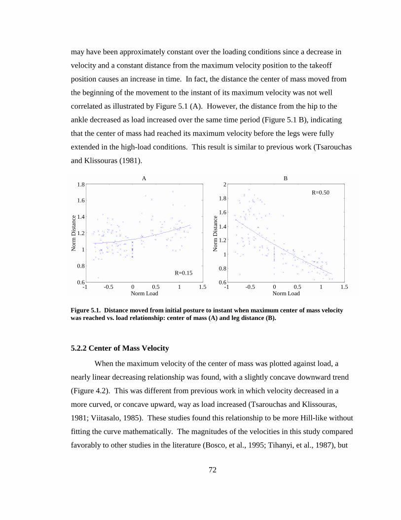
72
may have been approximately constant over the loading conditions since a decrease in
velocity and a constant distance from the maximum velocity position to the takeoff
position causes an increase in time. In fact, the distance the center of mass moved from
the beginning of the movement to the instant of its maximum velocity was not well
correlated as illustrated by Figure 5.1 (A). However, the distance from the hip to the
ankle decreased as load increased over the same time period (Figure 5.1 B), indicating
that the center of mass had reached its maximum velocity before the legs were fully
extended in the high-load conditions. This result is similar to previous work (Tsarouchas
and Klissouras (1981).
5.2.2 Center of Mass Velocity
When the maximum velocity of the center of mass was plotted against load, a
nearly linear decreasing relationship was found, with a slightly concave downward trend
(Figure 4.2). This was different from previous work in which velocity decreased in a
more curved, or concave upward, way as load increased (Tsarouchas and Klissouras,
1981; Viitasalo, 1985). These studies found this relationship to be more Hill-like without
fitting the curve mathematically. The magnitudes of the velocities in this study compared
favorably to other studies in the literature (Bosco, et al., 1995; Tihanyi, et al., 1987), but
Figure 5.1. Distance moved from initial posture to instant when maximum center of mass velocity was reached vs. load relationship: center of mass (A) and leg distance (B).
-1 -0.5 0 0.5 1 1.50.6
0.8
1
1.2
1.4
1.6
1.8 A
Norm Load
Nor
m D
ista
nce
R=0.15
-1 -0.5 0 0.5 1 1.50.6
0.8
1
1.2
1.4
1.6
1.8
2B
Norm Load
Nor
m D
ista
nce
R=0.50
73
Tsarouchas and Klissouras (1981) reported much higher velocities for both loaded and
unloaded jumps.
5.2.3 Ground Reaction Force
The maximum ground reaction force increased with increasing external load
(Figure 4.5) and the force-time curves were similar to that reported in the literature
(Tsarouchas and Klissouras, 1981). As illustrated by Figure 4.3, these maximums always
occurred late in the movement after an initial rise, followed by a leveling off, or decrease,
then the final rise to the peak. The maximum and average rates of force production both
decreased with increased load (Figure 4.4). Maximum rate of force production occurred
at different points in the movement for different subjects and for different conditions,
sometimes during the first force rise, sometimes during the second. This may explain
why the data is noisier for the maximum rate of force production as compared to the
average. Maximum rates of force production occurring at different times may be an
indication of different styles of jumping between subjects, or it could show that some of
the subjects could not consistently perform the jumping task over the range of loads.
Since the time of the performance and the maximum ground reaction force both increased
as load increased, and the time of maximum force was always late in the movement, it
makes sense that the average rate of force production should decrease with load as well.
The dual peak in the ground reaction force-time curve is a typical feature in many
vertical jump studies with much discussion as to what causes this phenomenon. One
popular explanation is that the initial peak is due to the extension of the hips (i.e. raising
of the trunk) and that the other peak is due to the extension of the legs (Miller and East,
1976). This study lends some support to this idea since the double peak seems to
decrease and eventually almost disappear with more and more unloading for some
subjects. In the loaded conditions, the weight was placed on the subject’s shoulders. If
the initial peak is due to the raising of the trunk, the initial peak should be more
pronounced since the mass of the trunk plus the load is increased. In the unloaded
conditions, the elastic bands were attached to the subject at the upper part of the back.
More upward band force would assist the trunk in moving upward and would decrease
the amount of force needed to raise the trunk when compared to the loaded jumps. The
74
initial peak should then be less pronounced. The data in the current study certainly does
not show these trends conclusively, but may lend support to a common theory. However,
the time of maximum center of mass velocity occurs later in the movement than the
maximum leg extension velocity implying that the legs extend first, then the trunk (see
Section 5.7.1). This ‘conflict’ could be a potential avenue for future research.
The ground reaction force that corresponded with the instant of maximum
velocity increased linearly with increased load (Figure 4.5). This is similar to data
reported by Nelson and Martin (1985). This is not surprising since the two parameters
are closely related and in fact only differ by the body weight of the particular subject as
stated earlier. The ranges for ground reaction force in the loaded configuration are
consistent with other studies in the literature (Tihanyi, et al., 1987; Bosco and Komi,
1979; Viitasalo, 1985). Very few researchers have examined unloaded jumping, but the
ranges in this study are greater than Tsarouchas and Klissouras (1981) who unloaded to
about 50% of bodyweight.
5.2.4 Knee Angular Velocity and Leg Extension Velocity
The maximum knee angular velocity-load relationship was very scattered, but
indicated a generally decreasing, concave downward shape (Figure 4.6). This was
different than previously reported data in vertical jumping, which was reported to be
more Hill-like, with concave upward curves (Bosco and Komi, 1979;Viitasalo, 1985);
although Bosco and Komi (1979) fit their curve by hand and their data were not clearly
concave upward and could possibly be favorably compared to this study. Leg extension
velocity had not been previously reported in the literature, but it appeared to be an easy
and reliable way to report extension velocity of the knee joint in a vertical jump. Leg
extension velocity decreased nearly linearly with increased load, following the trend of
the center of mass velocity (Figure 4.7 A). Once again, the curve was not as Hill-like as
expected.
Knee angular velocity was expected to closely follow other velocity patterns since
the knee extensors are sometimes considered the main muscle movers in the vertical
jump. Bosco and Komi (1979) assumed this to be true and simply plotted average ground
reaction force (assumed to be closely related to the knee extensor force) and average knee
75
angular velocity measured with a goniometer for vertical jumps with various additional
loads.
5.2.5 Knee Moment
Knee moment corresponding to the maximum knee angular velocity did not
appear to change in any discernable pattern as load increased (Figure 4.7 B). This result
is probably due to the fact that knee moment is affected a great deal by the posture and
the coordination of force production in a multi-joint movement such as the vertical jump.
The subjects were most likely in a slightly different position at the instant of maximum
knee angular velocity in each condition. Even if the maximum angular velocity occurred
at a predictable time in the movement (which it did), the knee moment could vary a great
deal. This effect can be greatly exaggerated by additional weight on the shoulders of the
subjects (Zatsiorsky, 1995). Possibly because of this effect, knee moment has not been
reported in the vertical jump force-velocity literature, but it is very common in the single-
joint literature (see Section 2.1.3.3). Please refer to Section 5.6.3 for a more detailed
discussion on joint moments and position affects.
5.2.6 EMG
EMG was originally planned to be a large part of this experiment, but full analysis
proved to be beyond the reasonable scope of the project. Therefore only two subjects
were analyzed and the data for the most loaded, bodyweight, and most unloaded
conditions were presented in Figure 4.8 and Appendix A. The loading did not appear to
change the activation patterns to a great extent within a subject, but the gluteus maximus
seemed to be activated earlier and more continuously in Subject B. The leg extensors
(rectus femoris and vastus lateralis) appeared to be the main muscles in use during the
movement for Subject A. They were involved for nearly the entire movement, except
near the end where the grastrocnemius, gluteus maximus and the biceps femoris became
more prevalent. This seems to corroborate the work of several researchers who studied
the role of biarticular muscles in the vertical jump (Prilutsky and Zatsiorsky, 1994;
Bobbert, et al., 1986; van Soest, et al., 1993; van Leeuwen and Spoor, 1992; Jacobs, et
al.,1996; Gregoire, et al., 1984). They have shown that the force produced in the knee
76
extensors can be transferred to the hip and ankle extensors and vice versa through the
biarticular knee and flexors and ankle extensors (hamstring and calf muscles).
A common theory is that the force in vertical jumping is transferred from the
proximal joints to the distal ones, i.e. the hip extensors act first, then the knee extensors,
then finally the ankle extensors (Bobbert and van Ingen Schenau, 1988). From a cursory
look at a limited amount of EMG data it appears that the knee extensors act first and then
the hip and ankle extensors are used primarily near the end of the movement for one
subject, but the knee and hip extensors seemed to work more concurrently in the other
subject. There appears to be more than one effective pattern of activation in the vertical
jump. This could be a direction for future research.
It is important to remember that EMG signal strength varies depending on the
depth of the muscle, the skin thickness, and the quality of the electrode application so
relative strength of signal does not necessarily indicate level of muscle activation. This
discussion was limited to activation timing and sequences. A more detailed study of
these patterns is required before more definitive conclusions can be made.
This section discussed how and why the main variables in this study varied with
changes in external load. The experimental protocol and procedures were shown to be
adequate enough to produce the widest range of forces and velocities seen in the literature
for vertical jumping. Nearly all of the variables chosen for discussion varied in a
predictable way as load varied, however, several variables were shown to be poor choices
for force-velocity study due to possible joint position affects.
5.3 Parameter Combinations for Studying Force-Velocity Relationships
This section discusses the results of combining the previously discussed variables
in the most informative ways that illustrate the force-velocity characteristics of the
vertical jump under varied loading conditions. As has been mentioned previously, the
choices for the selection of variables in parametric, multi-joint, force-velocity studies are
innumerable. This study is no exception. Although many parameter combinations were
examined in this study, several of them were rejected when no discernable trends were
seen, e.g. knee moment vs. knee angular velocity, or if the parameters did not seem to
77
add to the analysis, e.g. maximum force vs. maximum velocity (see Results for details).
These results will not be included in the discussion.
The only truly independent variable in this experiment was external load. All
other calculated variables are dependent on external load, so combinations involving
these parameters indicate relationships only; cause and effect cannot be implied. The
following relationships will be discussed: 1) ground reaction force corresponding to the
instant of maximum center of mass velocity vs. maximum center of mass velocity, 2)
ground reaction force corresponding to the instant of maximum knee angular velocity vs.
maximum knee angular velocity, and 3) ground reaction force corresponding with the
instant of maximum leg extension velocity vs. leg extension velocity.
5.3.1 Ground Reaction Force vs. Center of Mass Velocity
The corresponding ground reaction force when plotted with the maximum
velocity of the center of mass had two patterns across the subjects (Figure 4.9 A and B).
Most of the subjects produced concave downward trends, which shows up in the
normalized, combined plot (Figure 4.9 C). A few of the subjects had a concave upward
trend. The concave upward trend is consistent with the results previously reported in the
literature (Tsarouchas and Klissouras, 1981; Tihanyi, et al., 1987) and with Hill-like
curves (see below), but the concave downward trend differs from most of the literature.
Bosco, et al. (1995) found linear average force-velocity relationships. Wit, et al. (1993)
found that the isokinetic knee flexion torque and angular velocity relationship was
slightly concave downward for one group of subjects. This was the only favorably
comparing result found in the literature.
5.3.2 Ground Reaction Force vs. Knee Angular Velocity and Leg Extension Velocity
Corresponding ground reaction force when plotted with maximum knee angular
velocity and leg extension velocity both indicated decreasing, slightly concave upward
relationships (Figure 4.11). These showed the same trends as previously reported results
in the literature (Bosco and Komi, 1979) and were more Hill-like than the force-velocity
relationship reported above. The selection of knee angular velocity assumed that the leg
extensors were the primary mover in the vertical jump and that the angular velocity of the
78
knee joint was related to the linear velocity of shortening of the leg extensors. Since the
leg extensors were assumed to be the primary muscle group, the vertical ground reaction
force was assumed to be related to the force production in the leg extensors (Bosco and
Komi, 1979). This is corroborated on some level by the EMG results discussed above.
This section showed that the corresponding ground reaction force vs. center of
mass velocity relationship did not compare favorably with the prevailing literature, but
that ground reaction force vs. knee angular velocity and extension velocity relationships
compared favorably to much of the force velocity literature for multi-joint movements.
5.4 Force Plate and Video Method Comparison
This part of the project came about as a result of the need to combine force plate
and video data in order to calculate parameters such as knee moment and knee power.
Theoretically, all of the parameters calculated with either method should be the same.
However, in actual practice it is rare for digitized video data to accurately reproduce
force plate and velocity data except in very simple, slow movements. Data acquired from
video tends to be comparatively noisy and therefore requires significant filtering which
can sometimes clip off real data during the filtering process. This study was dependent
on maximum values for the instant of analysis in each load condition, so the compromise
solution outlined in the Methods was used because clipping of the data was undesirable.
The analysis process required the data to be differentiated twice in order to calculate
linear and angular acceleration. This process magnified any noise artifacts, making the
acceleration data, and therefore the calculated ground reaction force, more unreliable than
direct measurement from a force plate.
Despite the aforementioned complications, when single data points from each
loading condition were selected and combined to form the parametric load-velocity and
force-velocity relationships for each subject, both methods produced very similar results
(most of the intra-class correlation coefficients were 0.9 or above). The video data was
consistently lower at any given instant than the force plate data for both maximum center
of mass velocity and ground reaction force; but when the data was normalized, the two
methods produced nearly identical results. Interestingly, the video data produced a
79
ground reaction force-center of mass velocity relationship that was more Hill-like than
the plot produced with the ground reaction force data. The fact that the two methods
tended to agree was important because the methods involving the inverse dynamics
analysis of the knee joint used a combination of force plate data and differentiated video
position data to calculate knee moment.
5.5 Comparisons to Hill’s Curve
As has been mentioned in the previous sections, the force-velocity and velocity-
load curves from this study in many cases differed qualitatively from those published in
the literature. All of the authors of vertical jump force-velocity studies indicated that
parametric force-velocity relationships in vertical jumping under varying load were Hill-
like except Bosco, et al. (1995), who showed a more linear result. As previously
described, Hill-like curves were defined as a descending, concave upward curve with the
a/Fo ratio between zero and one. This relationship is often fit hyperbolically with Hill’s
curve to analytically describe the data. All of the force-velocity relationships in this
study were descending curves, as expected. However, an initial fit with simple second-
degree polynomials indicated that several of the curves were not Hill-like in that they
tended to be concave downward, not concave upward.
In spite of their visual differences from the classical Hill curves, all of the relevant
curves in this study were approximated with Hill’s force-velocity equation and the
appropriate constants were calculated and reported in the Results. In the cases where the
initial polynomials were concave upward (corresponding ground reaction force vs.
maximum center of mass velocity (video), vs. maximum angular velocity, and vs. leg
extension velocity), the Hill’s fit was nearly identical to initial fit and the correlation
coefficients reflected this (Table 4.1). In the other cases, the Hill fit was nearly linear and
did not fit the data quite as well as the polynomial did, as reflected by the correlation
coefficients (Table 4.1). The values for the constant a/Fo in these curves did not compare
favorably with the literature. Most authors who calculated a/Fo found their ratio to be
between zero and one (Jaric, et al., 1986; Tihanyi, et al., 1987; all other single
muscle/fiber studies) with a few exceptions. Ameredes, et al. (1992) found a/Fo ratios of
80
1.0 to 1.6 in the gastrocnemius of dogs, and Chow and Darling (1999) found a/Fo values
to typically be between zero and one, but reported values as high as 5.05 for the wrist
flexors. Therefore, it must be concluded that for the variable combinations described
above as concave downward and/or with the ratio a/Fo greater than one, Hill’s force-
velocity equation was not the best way to describe the data. As mentioned in the
previous chapters, Hill’s curve was just another way to describe the force-velocity
relationship and did not have any additional intrinsic meanings. Therefore, any other fit
that described the data best was satisfactory. The next section will discuss in detail the
possible theoretical reasons why multi-joint force-velocity curves may not follow the
classic force-velocity curve as described by Hill.
5.6 Theoretical Mechanical and Physiological Explanations
The previous sections have shown that the results of this study, for many of the
parameter combinations, were qualitatively different than the classical Hill’s curve. The
purpose of this section is to shed light on the possible reasons why this may have
happened from a theoretical, mechanical point of view. It was beyond the scope of this
project to attempt to create a model that would combine all of these factors to predict the
current results; however, it was constructive to analyze potential reasons for the
differences. Each critical point in the analysis will be discussed individually; then all
parts of the analysis will be combined, and the force and velocity will be traced from the
muscles to the effective force acting at the center of mass and the center of mass velocity.
Wilkie (1950) stated that some very strict guidelines should be followed when
studying parametric force-velocity relationships in human muscle:
1) Geometrically simple joint.
2) Movement should involve as few muscles as possible with a small distance
from the joint center to the muscle insertions.
3) The movement should not disturb the rest of the body.
4) The movement should be reproducible (i.e. easy task).
81
None of these requirements are fulfilled in loaded and unloaded vertical jumps: 1) not
only is there more than one joint involved, but the joints are complex and are extended at
different rates at different times, 2) the movement involves many muscles, both agonist
and antagonist, 3) the entire body moves, and 4) the results of the pilot studies indicated
that maximum center of mass velocity was reproducible over several trials, but that does
not imply that all of the parameters leading to the maximum velocity were exactly
reproduced from trial to trial (as can be seen by the distance that the center of mass
traveled during each of the trials (Figure 5.1 A), for example).
Intuitively, force should generally decrease as velocity increases as seen in
everyday experiences with weight lifting and other loaded movements. The results of the
current experiment confirmed this general relationship. However, it was not surprising
that the exact shape of the force-velocity curve was not the same as in single muscle/fiber
or single joint studies because all of the requirements listed by Wilkie could not be
controlled in multi-joint movements. Perhaps it is more surprising that, with a few
exceptions, most authors studying multi-joint force-velocity relationships have compared
their data favorably with Hill’s curve (see Section 5.5), despite the multi-joint problems.
The following sections identify and discuss the main factors in force-velocity
relationships and how they might contribute to differences between Hill-like curves in
simpler models and non-Hill-like curves in the present multi-joint movements. The main
factors to be discussed are 1) muscular factors, 2) factors involving individual and
multiple joints, and 3) factors involving joint position.
5.6.1 Muscular Factors
This analysis starts with the assumption that every muscle involved has a typical
Hill-like force-velocity curve if tested in a controlled laboratory situation, and that this
relationship would be manifested during a complex movement. Obviously, a vertical
jump is not a controlled laboratory situation for each muscle, so potential complications
exist that can change how the intrinsic force-velocity relationships are seen externally.
82
5.6.1.1 Muscle Length
A well-known property of muscles is that the force producing capability of a
particular muscle changes with changes in muscle length (Askew, et al., 1998; Chapman,
1974; Granzier, et al., 1989; Kaufman, et al., 1989; Kornecki and Siemienski, 1995).
Some factors that contribute to the force-length characteristics are the number of active
actin and myosin cross bridges that are overlapped at a given muscle length, and the
structure of the muscle (i.e. whether the muscle has a few long fibers or many short fibers
arranged in parallel with each other, pennation angle, etc.) (Baratta, et al., 1995;
Kaufman, et al., 1989). Force-velocity investigators often attempt to control this issue by
collecting data at specific muscle lengths or joint angles so that the muscle is in the same
configuration over the various loading conditions. The effect of joint configuration on
muscle length is discussed in more detail in Section 5.6.2.1.
Controlling the precise body position and, therefore, the exact muscle lengths,
was extremely difficult if not impossible in multi-joint movements. This was shown in
this study by Figure 5.1 (B), which indicated that the knee joint was in a different
position at the instant of maximum center of mass velocity under different loading
conditions. Since the body position at the instant of maximum velocity was not
consistent across all of the loading conditions, it could contribute to a change in the
appearance of the force-velocity curve since the muscles would not have been in the same
configuration for each trial.
5.6.1.2 Muscle Prestretch
If the muscle is stretched while it is stimulated, the force output of the contractile
components increases. In addition, sudden additions of force can cause the passive
structures of the muscle (the series elastic component) to stretch and slightly delay the
force production of the muscle. Prestretch often occurs during movements in which the
direction of motion is reversed, often characterized as the stretch-shortening cycle, and
has been a hot topic for investigation (e.g. Fukashiro, et al., 1983; Cavagna, et al., 1968;
Cavagna, 1977; Assmussen and Bonde-Petersen, 1974; Anderson and Pandy, 1993;
Alexander and Bennet-Clark, 1977). Investigators studying force-velocity characteristics
83
of muscle have attempted to control prestretch by trimming off all connective tissue
possible in single muscle/fiber preparations, and/or by only allowing concentric muscle
actions during the experiments, thus avoiding prestretch or force delays altogether.
The present study attempted to control the prestretch issues by using
noncountermovement vertical jumps. However, the muscles were statically loaded and
were activated as the subjects assumed the jumping position, especially in the high
loading conditions and not as much in the very unloaded conditions. This disparity could
contribute to changes in the force-velocity relationship across loading conditions. This
will be discussed in more detail in the following section.
5.6.1.3 Quick Release vs. No Quick Release Methods
A quick release technique was used in many single fiber/muscle and single-joint
force-velocity experiments (see ‘QR’ column in Tables 2.1-2.5). In this type of
procedure, the muscle was statically preactivated to a predetermined level in the starting
position, then the fiber/muscle/limb was suddenly released to a lower force level during
the movement. This technique is used for several reasons. First, it allows the
fiber/muscle(s) to be more fully activated during the movement and reduces the
acceleration to maximum velocity period as the fiber/muscle/limb is released from the
resting position. In low load situations, the fiber/muscle(s) may actually move through
the entire contraction distance before the maximum force and/or velocity is reached.
Second, because the fiber/muscle(s) are preactivated it reduces the time for the
fiber/muscle(s) to produce force, take up whatever slack there may be in the system, and
reach maximum activation levels. Third, it prestretches the series elastic component to
reduce force production delay.
Quick release techniques were not used in the present experiment. This means
that the muscles were preloaded at different levels and presumably activated at different
levels before the movement began. The subjects were forced to accelerate from zero
velocity to maximum velocity without the benefit of similar muscular preactivation
across the external loading conditions. This could affect the force-velocity relationship if
the maximum force or velocity theoretically possible was not achieved during the time of
the movement, as stated in the previous section. For a given level of unloading, an
84
increase in the center of mass velocity could make the velocity-load curves, and similarly
the force-velocity curves since force and load are closely related, more Hill-like. A quick
release-type procedure may have addressed some of these concerns, but it would add
some complications to the calculations. This may be an avenue for future investigation.
5.6.1.4 Instantaneous Muscle Force and Velocity
In classic studies of muscle force-velocity relationships, either the force that the
muscle must produce or the velocity of the contraction is controlled and ideally kept
constant during a trial. This can be accomplished very nicely in single muscle fiber
preparations with sophisticated machinery. In studies involving humans, constant muscle
force and/or velocity is not valid, even in single-joint studies that control the external
force or the movement velocity. As the joint configurations change, the lengths of the
muscles vary, changing the force production. Additionally, because of the changes in
joint configuration and activation, the velocity of shortening of the muscle itself may not
be constant, even if the limb velocity (or joint angular velocity) is held constant. Joint
configuration will be discussed in more detail below.
In this vertical jump study, joint configuration was not controlled, nor was joint
velocity. This means that the force produced by individual muscles was not constant
throughout the movement despite the maximum effort of the subjects, and the individual
muscle shortening velocity was not constant throughout the movement. The choice of
maximum center of mass velocity did not insure that the maximum shortening velocity of
any given muscle in the legs occurred at that instant. These individual muscle force and
velocity factors may have contributed to the differences seen in the results compared to
Hill’s curve.
5.6.2 Individual and Multiple Joint Factors
Each joint in the body contributes a different set of conditions to the whole body
during each instant in the movement because of several factors: the geometry of the joint
and joint configuration, and the number and arrangement of muscles acting at the joint.
85
5.6.2.1 Joint Geometry and Joint Configuration
Each joint in the body has a particular geometry or shape. Where and how the
muscles are attached around the joint affect how a given level of muscular force at a
given instant in time will contribute to the joint moment. A certain muscle force should
theoretically produce a joint moment that is proportional to the effective moment arm of
the muscle in relation to the joint center. As the joint rotates, the configuration and the
geometry of the joint changes, altering the angles of muscle attachment and the effective
moment arms for the muscles. Therefore, even if a muscle produced a constant force
throughout the movement, the changing joint configuration would cause the moment
produced at the joint to change. As mentioned above, changing the joint configuration
can also change the length of the muscles, altering the amount of force the muscles are
able to produce at a given moment (e.g. An, et al., 1984; Brand, et al., 1982; Spoor, et al.,
1990).
These relationships can be written mathematically. In a simple case, the muscle
moment arm (d) is related in some predictable way as a function of joint angle (θ),
d = f1(θ), (1)
the force (F) produced by the muscle is also predicted by the joint angle,
F = f2(θ), (2)
and the moment (M) is related to the force by the size of the moment arm,
M = F x d. (3)
Combining,
M = f2(θ) x f1(θ). (4)
Similarly, the velocity produced at the muscle (V) can be expressed as some function of
the joint angle,
V = f3(θ), (5)
and the velocity produced at the muscle is related to the joint rotation velocity (ω) by the
size of the moment arm (d), or
ω = V/d. (6)
Combining,
ω = f3(θ)/f1(θ). (7)
86
Equations (4) and (7) show that the joint moments that produce rotation and the resulting
angular velocities at the joint are very complicated even for the simple situation of a
single joint with a single muscle.
When multiple joints are involved, the situation is further complicated by the fact
that the joint configurations of more than one joint are changing at once. This is
especially true when muscles span two joints. One joint could be attempting to shorten
the muscle, another could be attempting to lengthen the muscle, the overall length of the
muscle could be shortening, lengthening or remaining constant. The muscle would then
be contributing to the net moment of both joints.
Measuring the force and velocity at a specific joint angle for all conditions can
minimize the complications due to joint configuration in single joint studies since the
moment arm and the muscle length should be approximately the same. As mentioned
above, the choice of the instant of maximum center of mass velocity in this multi-joint
study did not guarantee constant joint configurations, nor did choosing a particular joint
angle to study since other joints may not have been at the same relative configuration
from trial to trial. It is easy to see how joint configuration could be a contributing factor
to the differences in the current study to classic Hill’s curves.
5.6.2.2 Number and Arrangement of Muscles
The net moment produced at a particular joint is complicated by the fact that there
are many muscles that cross most joints. Each one of these muscles has its own force-
velocity relationship. Each muscle is attached differently around the joint, therefore, the
same joint rotation can produce different effects in each muscle as the individual muscle
moment arms and lengths change. Each muscle then contributes to the net joint moment
differently at each instant in the movement.
An assumption that is often made in human force-velocity studies is that all of the
muscles involved in the motion are maximally activated during the entire movement.
Even for a single joint, this assumption is not always valid. Certain muscles can be
activated at different times during the movement. In multi-joint movement, simultaneous
activation almost never occurs. Many authors (Pandy and Zajac, 1991; van Ingen
Schenau, et al., 1992; Bobbert and van Ingen Schenau, 1988; Pandy, et al., 1990, van
87
Soest and Bobbert, 1993) have shown that the patterns of muscle activation in jumping
are very complex. Non-simultaneous activation is clearly seen with a cursory look at the
EMG results in this study (See Appendix A).
Net joint moment is also complicated by the action of antagonistic muscles.
These muscles produce forces that contribute moments in the opposite direction of the
movement, effectively reducing the net moment and confounding the interpretation of the
moment produced at the joint. Therefore, the force-velocity relationship of the individual
muscle could be hidden and would not show up in the movement of the entire body. In
loaded and unloaded vertical jumping, it is almost certain that antagonists are active for
balance and control. This is seen in the EMG results as well (see Appendix A). Multiple
joints complicate the matter even further. Two-joint muscles that seem to be antagonists
at one joint may actually contribute to the movement at another joint. If the muscle is
sufficiently activated to keep the muscle at nearly a constant length, movement at one
joint can actually be transferred to the next joint through the two-joint muscle (Prilutsky
and Zatsiorsky, 1994; Bobbert, et al., 1986; van Soest, et al., 1993; van Leeuwen and
Spoor, 1992; Jacobs, et al., 1996; Gregoire, et al., 1984).
5.6.3 Joint Position Factors
Joint position refers to the angle that two segments form at a joint. This differs
from joint configuration in this paper in that joint configuration refers to the changes
internal to the joint (i.e. muscle moment arms, angles of attachments, etc), whereas the
joint position ignores all of the internal properties. The positions of the joints, and
therefore the limb segments, themselves contribute to how force and velocity are
manifested at the end point of the limb. In this case, the endpoint that we are interested in
is the center of mass of the body. Of course, the center of mass is not an actual point on
the body, it is an imaginable point that can be calculated and is positioned in the body in
the trunk in the case of the vertical jump. The velocity of the center mass can be
calculated, and the force on the center of mass can be measured at the ground with a force
plate. It is assumed that the force measured at the force plate is equal to the force acting
at the center of mass.
88
The model that will be used in this section is called a basic body model or a stick
figure model. This model assumes that the body consists of rigid segments connected by
hinge joints. Moments at each joint are produced by an imaginary ‘torque motor’ that
replaces the muscles and the moment arms discussed above. The effects of all of the
factors discussed in the previous sections are lumped into the joint moment at each joint.
The lengths of all of the segments are assumed to remain constant. A three-link chain
will be assumed: the foot, the shank, and the thigh. The center of mass will be assumed
to be located at the hip at the endpoint of the chain, and the magnitude of the ground
reaction force at any given instant will be assumed to act at the hip. The instant of
maximum center of mass velocity is the instant of interest in this study for a given trial.
The endpoint force depends on the joint torques, and the joint configuration. This
can be shown mathematically by the equation,
T = JTF, (8)
where T is the matrix of joint torques, JT is the transpose of the Jacobian matrix, and F is
the matrix of endpoint forces. If the joint torques are known, the equation,
F = (JT)-1 T, (9)
is useful, where (JT)-1 is the inverse of the transverse Jacobian matrix. In certain
instances, the inverse of the Jacobian cannot be solved, for example when the legs are
fully extended, i.e. the leg segments are in a straight line. When the body approaches this
singular position, the legs can produce and support more force than at any other joint
position. The ground reaction forces in this study were maximal late in the movement
when the legs were approaching full extension. Tihanyi, et al. (1987) found that
isometric force could be produced at a level predicted by Hill’s force-velocity equation
only at joint positions that corresponded to the instant of maximum force production late
in the movement.
In a similar way, the angular velocities at the joints are related to the endpoint
velocity by the Jacobian matrix,
V = J ωωωω. (10)
There is no singularity in the Jacobian matrix in this instance since the inverse of the
matrix is not required, but in the case of leg extension, the ability of the subject to
89
transfer angular velocity to endpoint velocity is reduced the closer the legs get to full
extension.
If the force produced by the muscle is constant, and the effective moment arm of
the joint are assumed to constant (may not be a bad assumption if the muscle insertions
are a small distance from the joint center as Wilkie (1950) suggested) then the torque at
the joint is equal to the equation,
T = F x d, (11)
where d is the effective moment arm in the joint. This means that for this analysis, the
joint torque at each joint is constant. This enables the effects of the joint torques to be
separated from the joint position. If all of the joint torques are combined into one vector
T of constant magnitudes, the magnitude of this vector is, (T12 + T2
2 + … + Tn2)1/2, where
T12, T2
2, … , Tn2 are the magnitudes of the joint torque in each joint. A simple case is
when this magnitude is equal to one. Squaring eliminates the square root, and since the
square of the magnitude of a vector is the dot product of itself,
TTT=1. (12)
Substituting equation (8) into equation (12) yields,
FT JJT F = 1. (13)
This is the equation of an ellipse and represents an envelope of possible force vectors at
the endpoint of the segment chain. Actions in the direction of the major axis of the
ellipse are most effective, or ‘easiest’ to produce. Actions in the direction of the minor
axis of the ellipse are the most ‘difficult.’
Similarly, if the muscle shortening velocity is assumed to be constant and the
moment arm continues to be constant than the angular velocities at the joints will be
constant. Following the same logic as above, the magnitude of the angular velocity
vector is,
ωωωωTωωωω = 1, (14)
and substituting equation (10),
VT (J-1)T(J-1) V = 1. (15)
This represents the velocity ellipse with the same interpretation as above for the force
ellipse. Examples of possible force and velocity ellipses at different joint positions are
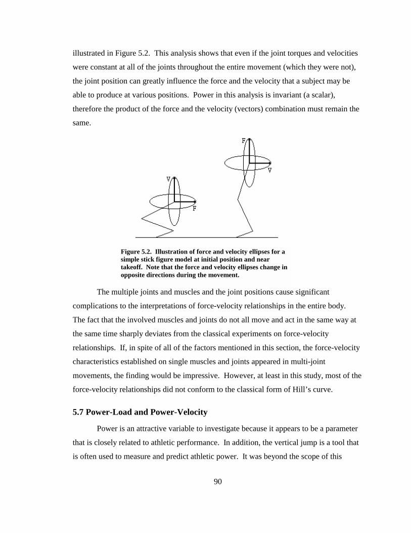
90
illustrated in Figure 5.2. This analysis shows that even if the joint torques and velocities
were constant at all of the joints throughout the entire movement (which they were not),
the joint position can greatly influence the force and the velocity that a subject may be
able to produce at various positions. Power in this analysis is invariant (a scalar),
therefore the product of the force and the velocity (vectors) combination must remain the
same.
The multiple joints and muscles and the joint positions cause significant
complications to the interpretations of force-velocity relationships in the entire body.
The fact that the involved muscles and joints do not all move and act in the same way at
the same time sharply deviates from the classical experiments on force-velocity
relationships. If, in spite of all of the factors mentioned in this section, the force-velocity
characteristics established on single muscles and joints appeared in multi-joint
movements, the finding would be impressive. However, at least in this study, most of the
force-velocity relationships did not conform to the classical form of Hill’s curve.
5.7 Power-Load and Power-Velocity
Power is an attractive variable to investigate because it appears to be a parameter
that is closely related to athletic performance. In addition, the vertical jump is a tool that
is often used to measure and predict athletic power. It was beyond the scope of this
Figure 5.2. Illustration of force and velocity ellipses for a simple stick figure model at initial position and near takeoff. Note that the force and velocity ellipses change in opposite directions during the movement.
91
investigation to debate the efficacy of the vertical jump and power measurements to
predict athletic power. In a nutshell, the commonly held theory is that the more power an
athlete can produce, the faster the athlete will tend to be and/or be able to deliver more
force in a shorter period of time. Thus, in athletic events that require these
characteristics, the better that athlete will be.
5.7.1 Shape of the Power Curve
Parametric power measurements in conjunction with force-velocity or velocity-
load experiments follow a typical shape. In force-velocity experiments that cover the
entire concentric range of forces and velocities, the power curve begins at zero power at
zero velocity/load/force, increases parabolically to a maximum value, and then decreases
to zero power at the maximum velocity/load/force. Since power can be calculated by
multiplying force and velocity, it is easy to see why this typical power curve exists. At
maximum load levels, the ability of the muscles to overcome the load is overcome, thus
there is no movement, i.e. zero velocity and zero power. At the other extreme, with no
load, velocity will be at a theoretical maximum, but will require no force to produce it,
thus zero power. Between these extremes intermediate values produce the increasing-
decreasing shape of the power curve.
As mentioned previously, it was impossible to cover the entire range of
theoretical loads, forces, and velocities for safety and other practical reasons in this
experiment. Therefore, it was interesting to identify where on the power curve this
experiment lay, i.e. on the ascending or descending portion of the curve. When looking
at the power-force and power-load curves, it appears that the power curve is in the
ascending range (Figure 4.17). This indicates that this experimental protocol included
much of the most unloaded portion of the theoretical power-load curve, but left out much
of the more loaded conditions that are theoretically possible. Logically, this makes the
power-velocity curve descending, which agrees with the results (Figure 4.18). These
curves seem to make sense, as the experiment could be safely undertaken in the unloaded
ranges until the subjects could not reach the ground, i.e. the elastic bands produced more
force than the weight of the subjects and they were suspended, unable to jump. However,
the experiment was stopped at the other extreme before the additional loads became
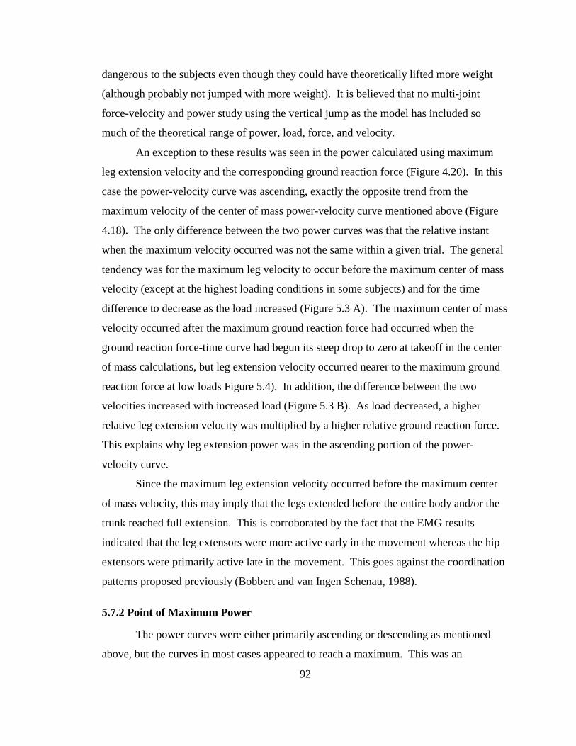
92
dangerous to the subjects even though they could have theoretically lifted more weight
(although probably not jumped with more weight). It is believed that no multi-joint
force-velocity and power study using the vertical jump as the model has included so
much of the theoretical range of power, load, force, and velocity.
An exception to these results was seen in the power calculated using maximum
leg extension velocity and the corresponding ground reaction force (Figure 4.20). In this
case the power-velocity curve was ascending, exactly the opposite trend from the
maximum velocity of the center of mass power-velocity curve mentioned above (Figure
4.18). The only difference between the two power curves was that the relative instant
when the maximum velocity occurred was not the same within a given trial. The general
tendency was for the maximum leg velocity to occur before the maximum center of mass
velocity (except at the highest loading conditions in some subjects) and for the time
difference to decrease as the load increased (Figure 5.3 A). The maximum center of mass
velocity occurred after the maximum ground reaction force had occurred when the
ground reaction force-time curve had begun its steep drop to zero at takeoff in the center
of mass calculations, but leg extension velocity occurred nearer to the maximum ground
reaction force at low loads Figure 5.4). In addition, the difference between the two
velocities increased with increased load (Figure 5.3 B). As load decreased, a higher
relative leg extension velocity was multiplied by a higher relative ground reaction force.
This explains why leg extension power was in the ascending portion of the power-
velocity curve.
Since the maximum leg extension velocity occurred before the maximum center
of mass velocity, this may imply that the legs extended before the entire body and/or the
trunk reached full extension. This is corroborated by the fact that the EMG results
indicated that the leg extensors were more active early in the movement whereas the hip
extensors were primarily active late in the movement. This goes against the coordination
patterns proposed previously (Bobbert and van Ingen Schenau, 1988).
5.7.2 Point of Maximum Power
The power curves were either primarily ascending or descending as mentioned
above, but the curves in most cases appeared to reach a maximum. This was an
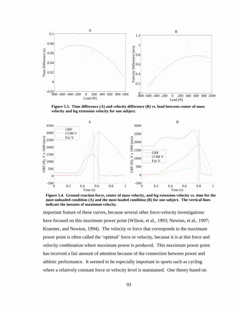
93
important feature of these curves, because several other force-velocity investigations
have focused on this maximum power point (Wilson, et al., 1993; Newton, et al., 1997;
Kraemer, and Newton, 1994). The velocity or force that corresponds to the maximum
power point is often called the ‘optimal’ force or velocity, because it is at this force and
velocity combination where maximum power is produced. This maximum power point
has received a fair amount of attention because of the connection between power and
athletic performance. It seemed to be especially important in sports such as cycling
where a relatively constant force or velocity level is maintained. One theory based on
-800 -600 -400 -200 0 200 400 600 800 1000-0.02
0
0.02
0.04
0.06
0.08
0.1 A
Load (N)
Tim
e D
iffer
ence
(s)
-800 -600 -400 -200 0 200 400 600 800 10000
0.2
0.4
0.6
0.8
1
1.2B
Load (N)
Vel
ocity
Diff
eren
ce (m
/s)
Figure 5.3. Time difference (A) and velocity difference (B) vs. load between center of mass velocity and leg extension velocity for one subject.
Figure 5.4. Ground reaction force, center of mass velocity, and leg extension velocity vs. time for the most unloaded condition (A) and the most loaded condition (B) for one subject. The vertical lines indicate the instants of maximum velocity.
0 0.2 0.4 0.6 0.8 1-500
0
500
1000
1500
2000
2500
3000
3500 A
Time (s)
GR
F (N
), V
x 1
000
(m/s
)
GRF COM V Ext V
0 0.2 0.4 0.6 0.8 1-500
0
500
1000
1500
2000
2500
3000
Time (s)
GR
F (N
), V
x 1
000
(m/s
)
B
GRF COM VExt V
94
optimal load promotes training at the loading level that produces maximum power; the
idea being that training at the point of maximum power will increase the maximum power
production of the athlete. This ‘optimum’ training level has been reported to be
approximately 33% of the maximum amount the athlete can move (Kraemer and Newton,
1994; Wilson, et al., 1993).
It was not possible to directly compare the maximum power points of this study
with the theoretical optimum proposed above because the exact shape of the power curve
in the force and velocity ranges not covered in this study are unknown. However, based
on the self-reported maximum squat lifts of the subjects, and the fact that maximum
power occurred at approximately 85% of the subjects’ body weight in additional loading,
maximum power occurred at approximately 37-61% of the maximum squat lifts of the
subjects. In addition, maximum power occurred at approximately 70% of the velocity of
a normal bodyweight jump. When the maximum velocity predicted by the power curve
calculated with the force plate data was used, maximum power corresponded to a velocity
of 56% of maximum achievable velocity. These measures appeared to be higher than the
theoretical ‘optimal’ load level reported in the literature, but were similar to the results
reported by Thomas, et al. (1995). Remember that the calculations for optimal load done
for the current study were simply rough estimates and based on self-reported maximum
squats. Some of the subjects had not done a maximum squat in some time before the
experiment and were estimating their current abilities.
5.8 Conclusions
Based on the results of this study and the preceding discussion, the following
conclusions corresponding to the original hypotheses for the experiments were as
follows:
1. Hill-like curves were defined as descending, concave upward curves with
the ratio a/Fo between zero and one. All of the velocity measures
(maximum center of mass using both video and force plate methods,
maximum knee angular velocity; and leg extension velocity) vs. load
produced velocity-load plots that had concave downward polynomial fits
95
which were different than Hill’s curve and a/Fo was greater than one as
well. Therefore, it was concluded that these curves were not Hill-like.
When the appropriate ground reaction force was plotted against the
same velocity variables, the ground reaction force vs. the maximum center
of mass velocity using the force plate and video methods failed to produce
curves that were Hill-like in form. Once again, force plate curve was
concave downward and a/Fo was greater than one. The video method
produced a curve that was concave upward, but a/Fo was greater than one.
It was concluded that these curves were not Hill-like. Ground reaction
force vs. maximum knee angular velocity and maximum leg extension
velocity were both Hill-like in appearance and had a/Fo ratios between
zero and one. It was concluded that these curves were indeed Hill-like.
None of the plots with the knee moment produced any
relationships at all and were decidedly not Hill-like.
2. When comparing the curves to each other, the ‘best’ force-velocity curves
in this study were ground reaction force vs. maximum center of mass
velocity (video) fit with either the Hill equation or the polynomial, the
maximum center of mass velocity vs. load (force plate and video) fit with
the polynomial, and maximum center of mass velocity vs. load (video) fit
with Hill’s force-velocity equation. All of these relationships had intra-
class correlation coefficients over 0.9. The best fit of all was the
corresponding ground reaction force vs. maximum center of mass velocity
(video) with the Hill fit.
3. Power calculated with the knee moment produced no relationship and
therefore did not conform to the theoretical power-velocity curve.
Power calculated by multiplying ground reaction force by the
maximum center of mass velocity and by the maximum leg extension
velocity produced power-velocity and power-load curves that were similar
to the theoretical parabolic ascending-descending curves. They did not
cover the entire range of theoretical data, but they did reach a peak. The
96
power vs. load and vs. ground reaction force both had good correlation
coefficients over 0.9.
4. The power-velocity curve calculated with the maximum center of mass
velocity was on the descending portion of the theoretical power-velocity
curve as expected, and the power-load curves were on the ascending
portion of the theoretical power-load curve, as expected. The power-
velocity curve calculated with the leg extension velocity was exactly the
opposite from what was expected. This power-velocity curve was on the
ascending portion of the curve and the power-load was slightly
descending. A provisional, hypothetical explanation of this controversy
has been suggested.
5. The load corresponding to the maximum power was calculated to be
approximately 37-61% of the reported maximum squat lifts of the subjects
and approximately 56% of the maximum velocity of the center of mass of
the subjects. These were higher than the theoretical maximum power load
of 33% of maximum strength and 33% of maximum velocity that was
expected.
97
Reference List Adamson, G. T. and Whitney, R. J. (1971) Critical appraisal of jumping as a measure of
human power. In Medicine and Sport, vol 6: Biomechanics II. (Edited by Vredenbregt, J., Eindhoven, and Wartenweiler, J.), pp. 208-211. Karger, Basel.
Alexander, R. McN. and Bennet-Clark, H. C. (1976) Storage of elastic strain energy in
muscle and other tissues. Nature. 265, 114-117. Ameredes, B. T., Brechue, W. F., Andrew G.M. and Stainsby, W. N. (1992) Force-
velocity shifts with repetitive isometric and isotonic contractions of canine gastrocnemius in situ. Journal of Applied Physiology. 73, 2105-2111.
Amiridis, I. G., Martin, A., Morlon, B., Cometti, G. and Hoecke, J. van. (1995)
Activation patterns during maximal voluntary knee extension in high-skilled and sedentary individuals. XVth Congress of the International Society of Biomechanics. (Edited by Hakkinen, K., Keskinen, K. L., Komi, P. V. and A. Mero), pp. 52-53. Jyvaskyla, Finland.
An, K. N., Takahashi, K., Harrigan, T. P. and Chao, E. Y. (1984) Determination of
muscle orientations and moment arms. Journal of Biomechanical Engineering. 106, 280-282.
Anderson, F. C. and Pandy, M. C. (1993) Storage and utilization of elastic strain energy
during jumping. Journal of Biomechanics. 26, 1413-1427. Aragon-Vargas, L. F. and Gross, M. M. (1997) Kinesiological factors in vertical jump
performance: differences among individuals. Journal of Applied Biomechanics. 13, 24-44.
Aragon-Vargas, L. F. and Gross, M. M. (1997) Kinesiological factors in vertical jump
performance: differences within individuals. Journal of Applied Biomechanics. 13, 45-65.
Arsac, L. M., Hautier, C. A., Lacour, J. R. and Belli, A. (1995) Effect of sprint training
on a cycle ergometer on the muscle power-velocity measured during cycling. XVth Congress of the International Society of Biomechanics. (Edited by Hakkinen, K., Keskinen, K. L., Komi, P. V. and Mero, A.), pp. 70-71. Jyvaskyla, Finland.
Askew, G. N. and Marsh, R. L. (1998) Optimal shortening velocity (V/Vmax) of skeletal
muscle during cyclical contractions: length-force effects and velocity-dependent activation and deactivation. Journal of Experimental Biology. 201, 1527-1540.
98
Assmussen G., Beckers-Bleukx, G., and Marechal, G. (1994) The force-velocity relation of the rabbit inferior oblique muscle; influence of temperature. Pflugers Archives. 426, 542-547.
Asmussen E. and Bonde-Petersen, F. (1974) Apparent efficiency and storage of elastic
energy in human muscles during exercise. Acta Physiologica Scandinavica. 92, 537-545.
Asmussen E. and Bonde-Petersen, F. (1974) Storage of elastic strain energy in skeletal
muscles in man. Acta Physiologica Scandinavica. 91, 385-392. Bahill, T. and Karnavas, W. (1991) The ideal baseball bat. New Scientist, 6 April, 26-31. Baltzopoulos, V. and Brodie, D. A. (1989) Isokinetic dynamometry: applications and
limitations. Sports Medicine. 8, 101-116. Bangart, J. J., Widrick, J. J. and Fitts, R. H. (1997) Effect of intermittent weight bearing
on soleus fiber force-velocity-power and force-pCa relationships. Journal of Applied Physiology. 82, 1905-1910.
Baratta, R. and Solomonow, M. (1991) The effect of tendon viscoelastic stiffness on the
dynamic performance of isometric muscle. Journal of Biomechanics. 24, 109-116. Baratta, R. V., Solomonow, M., Best, R., Zembo, M., and D’Ambrosia, R. (1995) Force-
velocity relations of nine load-moving skeletal muscles. Medical and Biological Engineering and Computing. 33, 537-564.
Baratta, R. V., Solomonow, M., Best, R., Zembo, M., and D’Ambrosia, R. (1995)
Architecture-based force-velocity models of load-moving skeletal muscles. Clinical Biomechanics. 10, 149-155.
Baron, R., Bachl, N., Petschnig, R., Tschan, H., Smekal, G. and Pokan, R. (1999)
Measurement of maximal power output in isokinetic and non-isokinetic cycling. A comparison of two methods. International Journal of Sports Medicine. 20, 532-537.
Bartosiewicz, G., Danielewicz, J., Gajewski, J., Trzaskoma, Z. and Witt, A. (1990)
Evaluation of strength-velocity characteristics in athletes. In Biomechanics of Human Movement: Applications in Rehabilitation, Sports, and Ergonomics. (Edited by Berme, N. and Cappozzo, A.), pp. 426-430. Bertec Corporation, Worthington.
Basmajian, J. V. and Blumenstein, R. Electrode placement in electromyographic
biofeedback. 369-382.
99
Bedi, J. F., Cresswell, A. G., Engel, T. J. and Nicol, S. M. (1987) Increase in jumping height associated with maximal effort vertical depth jumps. Research Quarterly for Exercise and Sport. 56, 11-15.
Beckers-Bleukx, G. and Marechal, G. (1989) Force-velocity relation and myosin
isozymes of rat muscles. Biomed Biochim Acta. 48, S412-S416. Blickhan, R. (1989) The spring-mass model for running and hopping. Journal of
Biomechanics. 22, 1217-1227. Bobbert, M. F., Gerritsen, K. G. M., Litjens, M. C. A. and Soest, A. J. van. (1995)
Explanantion of differences in jump height between countermovement and squat jumps. XVth Congress of the International Society of Biomechanics. (Edited by Hakkinen, K., Keskinen, K. L., Komi, P. V. and Mero, A.), pp. 110-111. Jyvaskyla, Finland.
Bobbert, M. F., Gerritsen, K. G. M., Litjens, M. C. A. and Soest, A. J. van. (1996) Why
is countermovement jump height greater than squat jump height? Medicine and Science in Sports and Exercise. 28,1402-1412.
Bobbert, M. F., Huijing, P. A., and Ingen Schenau, G. J. van. (1986) An estimation of
power output and work done by the human triceps surae muscle-tendon complex in jumping. Journal of Biomechanics. 19, 988-906.
Bobbert, M. F. and Ingen Schenau, G. J. van. (1988) Coordination in vertical jumping.
Journal of Biomechanics. 21, 249-262. Bobbert, M. F. and Ingen Schenau, G. J. van. (1990) Isokinetic plantar flexion:
experimantal results and model calculations. Journal of Biomechanics. 23, 105-119. Bobbert, M. F., and Soest, A. J. van. (1994) Effects of muscle strengthening on vertical
jump height: a simulation study. Medicine and Science in Sports and Exercise. 26, 1012-1020.
Bober, T., Putnam, C. A. and Woodworth, G. G. (1987) Factors influencing the angular
velocity of a human limb segment. Journal of Biomechanics. 20, 511-521. Bober, T., and Zawadzki, J. (1993) Pre-stretch phase characteristics and the effectiveness
of take-off in vertical jumping. In XIVth Congress of the International Society of Biomechanics. pp.190-191. Paris, France.
Bosco, C. (1990) Evaluation of athletes and ergometry. In Biomechanics of Human
Movement: Applications in Rehabilitation, Sports and Ergonomics. (Edited by Berme, N. and Cappozzo, A.), pp. 413-430. Bertec, Worthington.
100
Bosco, C., Belli, A., Astrua, M., Tihanyi, J., Pozzo, R., Kellis, S., Tsarpela, O., Foti, C., Manno, R. and Tranquilli, C. (1995) A dynamometer for evaluation of dynamic muscle work. European Journal of Applied Physiology. 70, 379-386.
Bosco, C., Luhtanen, P. and Komi, P. V. (1983) A simple method for measurement of
mechanical power in jumping. European Journal of Applied Physiology. 50, 273-282.
Bosco, C. and Komi, P. V. (1981) Influence of countermovement amplitude in
potentiation of muscular performance. In Biomechanics VII-A. (Edited by Morecki, A., Fidelus, K., Kedzior, K. and Wit, A.), pp.129-135. University Park Press, Baltimore.
Bosco, C. and Komi, P. V. (1979) Potentiation of the mechanical behavior of the human
skeletal muscle through prestretching. Acta Physiologica Scandinavica. 106, 467-472.
Bosco, C., Tihanyi, J., Komi, P. V., Fekete, G. and Apor, P. (1982) Store and recoil of
elastic energy in slow and fast types of human skeletal muscles. Acta Physiologica Scandinavica. 116, 343-349.
Bottinelli, R., Canepari, M., Pellegrino, M. A. and Reggiani, C. (1990) Force-velocity
properties of human skeletal muscle fibres: myosin heavy chain isoform and temperature dependence. Journal of Physiology. 495, 573-586.
Bottinelli, R. and Reggiani, C. (1995) Force-velocity properties and myosin light chain
isoform composition of an identified type of skinned fibres from rat skeletal muscle. Pflugers Archives. 429, 592-594.
Bottinelli, R., Schiaffino, S. and Reggiani, C. (1991) Force-velocity relations and myosin
heavy chain isoform compositions of skinned fibres from rat skeletal muscle. Journal of Physiology. 437, 655-672.
Brand, R. A., Crowninshield, R. D., Wittstock, C. E., Pedersen, D. R., Clark, C. R. and
Krieken, F. M. van. (1982) A model of lower extremity muscular anatomy. Journal of Biomechanical Engineering. 104, 304-310.
Brown, L. E. and Whitehurst, M. (2000) Load range. In Isokinetics in Human
Performance. (Edited by Brown, L. E.), pp. 97-121. Human Kinetics, Champaign. Buttelli, O.,Vandewalle, H. and Jouanin, J. C. (1999) Recovery of the torque-velocity
relationship after short exhausting cycling exercise. European Journal of Applied Physiology. 80, 249-251.
101
Buttelli, O.,Vandewalle, H., Jouanin, J. C., Seck, D. and Monod, H. (1997) Effects of aerobic exercise on the torque-velocity relationship in cycling. European Journal of Applied Physiology. 75, 499-503.
Buttelli, O.,Vandewalle, H. and Peres, G. (1996) The relationship between maximal
power and maximal torque-velocity using an electronic ergometer. European Journal of Applied Physiology. 73, 479-483.
Cabri, J. M. H. (1991) Isokinetic strength aspects of human joints and muscles. Critical
Reviews in Biomedical Engineering. 19, 321-259. Capmal, S. and Vandewalle, H. (1997) Torque-velocity relationship during cycle
ergometer sprints with and without toe clips. European Journal of Applied Physiology. 76, 375-379.
Carlson, F. D. and Wilkie, D. R. (1974) Muscle Physiology. Prentice-Hall, Englewood
Cliffs. Carmichael, W. L. and Dowling, J. J. (1996) Modeling of the foot to improve segment
power estimates in the vertical jump. Conference Proceedings: 20th Annual Meeting of the American Society of Biomechanics. pp. 259-260.
Cavagna, G. A. (1977) Storage and utilization of elastic energy in skeletal muscle.
Exercise and Sport Science Reviews. 5, 89-129. Cavagna, G. A., Dusman, B., and Margaria, R. (1968) Positive work done by a
previously stretched muscle. Journal of Applied Physiology. 24, 21-32. Cavagna, G. A., Komarek, L., Citterio, G., and Margaria, R. (1971) Power output of the
previously stretched muscle. In Medicine and Sport: Biomechanics II. (Edited by Vredenbrecht, J. and Wartenweiler, J.), pp. 159-167. Karger, Basel.
Chapman, A. E. (1974) The relation between length and the force-velocity curve of a
single linear muscel during flexion of the elbow. In Biomechanics IV. (Edited by Nelson, R. C. and Morehouse, C. A.), pp. 434-439. University Park Press, Baltimore.
Chow, J. W. and Darling, W. G. (1999) The maximum shortening velocity of muscle
should be scaled with activation. Journal of Applied Physiology. 86, 1025-1031. Claflin, D. R. and Faulkner, J. A. (1989) The force-velocity relationship at high
shortening velocities in the soleus muscle of the rat. Journal of Physiology. 411, 627-637.
102
Cole, G. T., Bogert, A. J, van den, Herzog, W. and Gerritsen, K. G. M. (1996) Modeling of force production in skeletal muscle undergoing stretch. Journal of Biomechanics. 29, 1091-1104.
Colomo, F., Pizza, L. and Scialpi, A. (2000) Force-velocity and unloaded shortening
velocity during graded potassium contractures in frog skeletal muscl fibres. Journal of Muscle Research and Cell Motility. 21, 9-19.
Constable, R., Thornhill, R. J., and Carpenter, D. R. (1994) Time-frequency analysis of
the surface EMG during maximum height jumps under altered-G conditions. Biomedical Sciences Instrumentation. 30, 69-74.
Cook, C. S. and McDonagh, M. J. (1996) Force responses to constant-velocity
shortening of electrically stimulated human muscle-tendon complex. Journal of Applied Physiology. 81, 384-392.
Curtin, N. A. and Edman, K. A. (1994) Force-velocity relation for frog muscle fibers:
effects of moderate fatigue and of intracellular acidification. Journal of Physiology. 475, 483-494.
Dern, R. J., Levene, J. M. and Blair, H. A. (1947) Forces exerted at different velocities in
human arm movements. American Journal of Physiology. 151, 415-437. De Ruiter, C. J., Jones, D. A., Sargeant, A. J. and Haan, A. de. (1999) The measurement
of force/velocity relationships of fresh and fatigued human adductor pollicis muscle. European Journal of Applied Physiology. 80, 386-393.
Desipres, M. (1976) Polyparametric study of the vertical jump. In Biomechanics V-B.
(Edited by Komi, P. V.), pp. 73-80. University Park Press, Baltimore. Dowling, J. J. (1992) The effect of muscle mechanics on human movement outcomes as
revealed by computer simulation. Human Movement Science. 11, 273-297. Dowling, J. J., MacDonald, J. R., Ioannidis, G. and Davison, K. S. (1995) Variability of
torque-angle-velocity relations in hill-type muscle models. In XVth Congress of the International Society of Biomechanics. (Edited by Hakkinen, K., Keskinen, K. L., Komi, P. V. and Mero, A.), pp. 234-235. Jyvaskyla, Finland.
Dowling, J. J. and Vamos, L. (1993) Identification of kinetic and temporal factors related
to vertical jump performance. Journal of Applied Biomechanics. 9, 95-110. Driss, T., Vandewalle, H. and Monod, H. (1998) Maximal power and force-velocity
relationships during cycling and cranking exercises in volleyball players. Correlation with the vertical jump test. Journal of Sports Medicine and Physical Fitness. 38, 286-293.
103
Dudley, G. A. and Djamil, R. (1985) Incompatibility of endurance- and strength-training
modes of exercise. Journal of Applied Physiology. 59, 1446-1451. Dudley, G. A., Harris, R. T., Duvousin, M. R., Hather, B. M. and Buchanan, P. (1990)
Effect of voluntary vs. artificial activation on the relationship of muscle torque to speed. Journal of Applied Physiology. 69, 2215-2221.
Edman, K. A. (1988) Double-hyperbolic nature of the force-velocity relation in frog
skeletal muscle. Advances in Experimental Medical Biology. 332, 643-652. Epstein, M. and Herzog, W. (1998) Theoretical Models of Skeletal Muscle: Biological
and Mathematical Considerations. Wiley, Chichester. Feltner, M., E., Fraschetti, D. R., Crisp, R. and Stewart, T. (1996) Arm motion on lower
extremity angular kinetics during countermovement vertical jumps. In: Annual Meeting Abstracts, American College of Sports Medicine, Medicine and Science in Sports and Exercise. 28, S46.
Fenn, W. O. and Marsh, B. S. (1935) Muscular force at different speeds of shortening.
Journal of Physiology. 85, 277-297. Ferretti, G., Gussoni, M., Di Prampero, E. and Cerretelli, P. (1987) Effects of exercise on
maximal instantaneous muscular power of humans. Journal of Applied Physiology. 62, 2288-2294.
Fleiss, J. L. (1986) The Design and Analysis of Clinical Experiments. John Wiley &
Sons, New York. Froese, E. A. and Houston, M. E. (1985) Torque-velocity characteristics and muscle
fiber type in human vastus lateralis. Journal of Applied Physiology. 59, 309-314. Fugel-Meyer, A. R., Mild, K. H. and Hornsten, J. (1982) Output of skeletal muscle
contractions: a study of iskinetic plantar flexion in athletes. Acta Physiologica Scandinavica. 115, 193-199.
Fuji, N. and Moriwaki, T. (1993) Effect of additional weight on muscular power and
performance in vertical jump motion. In XIVth Congress of the International Society of Biomechanics, pp. 432-433. Paris, France.
Fukashiro, S., Ohmichi, H., Kanehisa, H. and Miyashita, M. (1988) Utilization of stored
elastic energy in leg extensors. In Biomechanics VIII-A & B. (Edited by Matsui, H. and Kobayashi, H.), pp. 258-263. Human Kinetics, Champaign.
104
Funato, K., Matsuo, A., Ikegawa, S. and Fukunaga, T. (1995) Force-velocity characteristics between weightlifters and bodybuilders in mono- and multi-articular movements. XVth Congress of the International Society of Biomechanics. (Edited by Hakkinen, K., Keskinen, K. L., Komi, P. V. and Mero, A.), pp. 294-295. Jyvaskyla, Finland.
Gasser, H. S. and Hill A. V. (1924) The dynamics of muscular contraction. Proceedings
of the Royal Society of London, B. 96, 398-437. Genuario, S. E., and Dolgener, F. A. (1980) The relationship of isokinetic torque at two
speeds to the vertical jump. Research Quarterly for Exercise and Sport. 51, 593-598. Gollhofer, A. and Kyrolainen, H. (1991) Neuromuscular control of the human leg
extensor muscles in jump exercises under various stretch-load conditions. International Journal of Sports Medicine. 12, 34-40.
Granzier, H. L., Burns, D. H. and Pollack, G. H. (1989) Sarcomere length dependence of
the force-velocity relation in single frog muscle fibers. Biophysics Journal. 55, 499-507.
Gregoire, L., Veeger, H. E., Huijing, P. A. and Ingen Schenau, G. J. van. (1984) Role of
mono- and biarticular muscles in explosive movements. International Journal of Sports Medicine. 5, 301-305.
Gregor, R. J., Edgerton, V. R., Perrine, J. J., Campion, D. S. and DeBus, C. (1979)
Torque-velocity relationships and muscle fiber composition in elite female athletes. Journal of Applied Physiology. 47, 388-392.
Grieve, D. W. and Linden, J. van der. (1986) Force, speed, and power output of the
human upper limb during horizontal pulls. European Journal of Applied Physiology. 55, 425-430.
Gulch, R. W. (1994) Force-velocity relations in human skeletal muscle. International
Journal of Sports Medicine. 15, S2-S10. Haan, A. de. (1988a) Comparison of force-velocity characteristics obtained using
twitches and tetani from in situ rat skeletal muscles. Quarterly Journal of Experimental Physiology. 73, 131-133.
Haan, A. de. (1988b) The influence of stimulation frequency on force-velocity
characteristics of in situ rat medial gastrocnemius muscle. Experimental Physiology. 83, 77-84.
105
Harman, E. A., Rosenstein, M. T., Frykman, P. N. and Rosenstein, R. M. (1990) The effects of arms and countermovement on vertical jumping. Medicine and Science in Sports and Exercise. 22, 825-833.
Hartmann, U., Mader, A., Wasser, K. and Klauer, I. (1993) Peak force, velocity, and
power during five and ten maximal rowing ergometer strokes by world class female and male rowers. International Journal of Sports Medicine. 14, S42-S45.
Hatcher, D. D. and Luff A. R. (1985) Force-velocity properties of fast-twitch and slow-
twitch muscles of the kitten. Journal of Physiology. 367, 377-385. Hautier, C. A., Linossier, M. T., Belli, A., Lacour, J. R. and Arsac, L. M. (1996) Optimal
velocity for maximal power production in non-isokinetic cycling is related to muscle fibre type composition. European Journal of Applied Physiology. 74, 114-118.
Hawkins D. and Smeulders, M. (1999) An investigation of the relationship between hip
extension torque, hip extension velocity, and muscle activation. Journal of Applied Biomechanics. 15, 253-269.
Hawkins, D. and Smeulders, M. (1998) Relationship between knee joint torque, velocity,
and muscle activation: considerations for musculoskeletal modeling. Journal of Applied Biomechanics. 14, 141-157.
Hay, J. G., Dapena, J., Wilson, B. D., Andrews, J. G. and Woodworth, G. G. (1978) An
analysis of joint contributions to the performance of a gross motor skill. In Biomechanics VI-B. (Edited by Assmussen, E. and Jorgensen, K.), pp. 64-70. University Park Press, Baltimore.
Heckman, C. J., Weytjens, J. L. and Loeb, G. E. (1992) Effect of velocity and
mechanical history on the forces of motor units in the cat medial gastrocnemius muscle. Journal of Neurophysiology. 68, 1503-1515.
Hill, A. V. (1940) The dynamic constants of human muscle. Proceedings of the Royal
Society of London, B. 128, 263-274. Hill, A. V. (1970) First and Last Experiments in Muscle Mechanics. Cambridge
University Press, London. Hill, A. V. (1938) The heat of shortening and the dynamic constants of muscle.
Proceedings of the Royal Society of London, B. 126, 136-195. Hill, A. V. (1922) The maximum work and mechanical efficiency of human muscles,
and their most economical speed. Journal of Physiology. 56, 19-41.
106
Hill, A. V. (1956) The thermodynamics of muscle. British Medical Bulliten, 12, 174-176.
Hochmuth, G. and Marhold, G. (1977) The further development of biomechanical
principles. In Biomechanics VI-B. (Edited by Assmussen, E. and Jorgensen, K.), pp. 93-106. University Park Press, Baltimore.
Housh, D. J., Housh, T. J., Weir, J. P., Weir, L. L., Johnson, G. O. and Stout, J. R. (1995)
Anthropometric estimation of thigh muscle cross-sectional area. Medicine and Science in Sports and Exercise. 27, 784-791.
Hubley, C. L. and Wells, R. P. (1983) A work-energy approach to determine individual
joint contributions to vertical jump performance. European Journal of Applied Physiology. 50, 247-254.
Ikegawa, S., Okada, J., Kawakami, Y. and Fukunaga, T. (1995) Force-velocity
characteristics of various muscle groups in humans. XVth Congress of the International Society of Biomechanics. (Edited by Hakkinen, K., Keskinen, K. L., Komi, P. V. and Mero, A.), pp. 418-419. Jyvaskyla, Finland.
Ingen Schenau, G. J. van. (1984) An alternative view of the concept of utilization of
elastic energy in human movement. Human Movement Science. 3, 301-336. Ingen Schenau, G. J. van, Bobbert, M. F., Huijing, P. A. and Woittiez, R. D. (1985) The
instantaneous torque-angular velocity relation in plantar flexion during jumping. Medicine and Science in Sports and Exercise. 17, 422-426.
Ingen Schenau, G. J. van, Boots, P. J., Groot, G. de, Snackers, R. J. and Woensel, W. W.
L. M. van. (1992) The constrained control of force and position in multi-joint movements. Neuroscience. 46, 197-207.
Jacobs, R., Bobbert, M. F., and Ingen Schenau, G. J. van. (1993) Function of mono- and
biarticular muscles in running. Medicine and Science in Sports and Exercise. 25, 1163-1173.
Jacobs, R., Bobbert, M. F., and Ingen Schenau, G. J. van. (1996) Mechanical output from
individual muscles during explosive leg extensions: the role of biarticular muscles. Journal of Biomechanics. 29, 513-523.
Jaric, S., Ristanovic, D. and Corcos, D. M. (1989) The relationship between muscle
kinetic parameters and kinematic variables in a complex movement. European Journal of Applied Physiology. 59, 370-376.
Jaric, S., Ristanovic, D., Gavrilovic, P. and Ivancevic, V. (1986) A new method for
determining the force-velocity relationship in human quadriceps muscle. In
107
Biomechanics IX-A. (Edited by Winter, D. A.), pp. 82-85. Human Kinetics Publishers, Champaign.
Jaskolska, A., Goossens, P., Veenstra, B., Jaskolski, A. and Skinner, J. S. (1999)
Comparison of treadmill and cycle ergometer measurements of force-velocity relationships and power output. International Journal of Sports Medicine. 20, 192-197.
Jenson, J. L., Phillips, S. J. and Clark, J. E. (1994) For young jumpers, differences are in
the movement’s control, not its coordination. Research Quarterly for Exercise and Sport. 65, 258-268.
Johansson, C., Lorentzon, R., Sjostrom, M., Fagerlund, M. and Fugl-Meyers, A. R.
(1987) Sprinters and Marathon Runners. Does isokinetic knee extensor performance reflect muscle size and structure? Acta Physiologica Scandinavica. 130, 663-669.
Jones, N., L., McCartney, N. and McComas, A., J., eds. (1986) Human Muscle Power.
Human Kinetics Publishers, Champaign. Jorgensen, K. (1976) Force-velocity relationships in human elbow flexors and extensors.
Biomechanics V-A. (Edited by Komi, P.), pp. 145-151. University Park Press, Baltimore.
Jorgenson, K. and Bankov, S. (1971) Maximum strength of elbow flexors and extensors
with pronated and supinated forearm. In Biomechanics II. (Edited by Vredenbregt, J. and Wartenweiler, J.), pp. 174-180. Basel, Karger.
Kannus, P. (1994) Isokinetic evaluation of muscular performance: implications for
muscle testing and rehabilitation. International Journal of Sports Medicine. 15, S11-S18.
Katz, B. (1939) The relation between force and speed in muscular contraction. Journal
of Physiology. 96, 45-64. Kaufman, K. R., An, K. and Chau, E. Y. S. (1989) Incorporation of muscle architecture
into the muscle length-tension relationship. Journal of Biomechanics. 22, 943-948. Kojima, T. (1991) Force-velocity relationship of human elbow flexors in voluntary
isotonic contraction under heavy loads. International Journal of Sports Medicine. 12, 208-213.
Komi, P.V. (1973) Measurement of the force-velocity relationship in human muscle
under concentric and eccentric contractions. In Medicine and Sport, Biomechanics III, 8, 224-229.
108
Komi, P. V. (1990) Relevance of in vivo force measurements to human biomechanics. Journal of Biomechanics. 23, 23-34.
Komi, P. V. and Bosco, C. (1978) Utilization of stored elastic energy in leg extensor
muscles by men and women. Medicine and Science in Sports. 10, 261-265. Koning, F. L. de, Binkhorst, R. A., Vos, J. A. and Hof, M. A. (1985) The force-velocity
relationship of arm flexion in untrained males and females and arm-trained athletes. European Journal of Applied Physiology. 54, 89-94.
Kornecki, S. and Siemienski, A. (1995) The influence of the muscle force-length
relationship on the shape of the force-velocity characteristics. XVth Congress of the International Society of Biomechanics. (Edited by Hakkinen, K., Keskinen, K. L., Komi, P. V., and Mero, A.), pp. 500-501. Jyvaskyla, Finland.
Kornecki, S. and Siemienski, A. (1998) Force-velocity characteristics of individual
human skeletal muscles: TBClat and TBClong. Outline of the method. International Journal of Occupational Safety and Ergonomics. 4, 75-83.
Kraemer, W. J. and Newton, R. U. (1994) Training for improved vertical jump.
Gatorade Sports Science Institute, Sports Science Exchange, Vol. 7, No.6. Kues, J. M. and Mayhew, T. P. (1996) Concentric and eccentric force-velocity
relationships during electrically induced submaximal contractions. Physiotherapy Research International. 1, 195-204.
Kunz, H. R. (1974) Effects of ball mass and movement pattern on release velocity in
throwing. In Biomechanics IV. (Edited by Nelson, R. C. and Morehouse, C. A.), pp. 163-168. University Park Press, Baltimore.
Lannergren, J. and Westerblad, H. (1989) Maximum tension and force-velocity
properties of fatigued, single Xenopus muscle fibres studied by caffeine and high K+. Journal of Physiology. 409, 473-490.
Leemputte, M. van, Spaepen, A. J., and Willems, E. J. (1987) Effect of the contraction
history on the force-velocity relation of elbow flexors. In Biomechanics X-A. (Edited by Jonsson, B.), pp. 271-276. Human Kinetics, Champaign.
Leeuwen, J., L. van and Spoor, C., W. (1992) On the role of biarticular muscles in
human jumping. Journal of Biomechanics. 25, 207-209. Leva, P. de. (1996) Adjustments to Zatsiorski-Seluyanov’s segment inertia parameters.
Journal of Biomechanics. 29, 1223-1230.
109
Levin, A. and Wyman, J. (1927) The viscous elastic properties of muscle. Proceedings of the Royal Society of London, B. 101, 218-243.
Lieber, R. L. (1992) Skeletal Muscle Structure and Function. Williams and Wilkins,
Baltimore. Linossier, M. T., Dormois, D., Fouquet, R., Geyssant, A. and Denis, C. (1996) Use of the
force-velocity test to determine the optimal braking force for a sprint exercise on a friction-loaded cycle ergometer. European Journal of Applied Physiology. 74, 420-427.
Loose, M. P. de, Bussman, J. B. J., Kingma, I. and Toussaint, H. M. (1992) Different
methods to estimate total power and its components during lifting. Journal of Biomechanics. 25,1089-1095.
Lou, F. and Sun, Y. B. (1993) The high-force region of the force-velocity relation in frog
skinned muscle fibres. Acta Physiologica Scandinavica. 148, 243-252. Luhtanen, P. and Komi, P. V. (1978) Segmental Contribution to forces in vertical jump.
European Journal of Applied Physiology. 38, 181-188. MacIntosh, B. R., Neptune, R. R., and Horton, J. F. (2000) Cadence, power, and muscle
activation in cycle ergometry. Medicine and Science in Sports and Exercise. 32, 1281-1287.
Malmquist, U. and Arner, A. (1996) Regulation of force and shortening velocity by
calcium and myosin phosphorylation in chemically skinned smooth muscle. Pflugers Archives. 433, 42-48.
Marechal, G. and Beckers-Bleukx, G. (1993) Force-velocity relation and isomyosins in
soleus muscles from two strains of mice (C57 and NMRI). Pflugers Archives. 424, 478-487.
Marshall R. N., Mazur, S. M. and Taylor, N. A. S. (1990) Three-dimensional surfaces
for human muscle kinetics. European Journal of Applied Physiology. 61, 263-270. Martin, A., Martin, L. and Morlon, B. (1995) Changes induced by eccentric training on
force-velocity relationships of the elbow flexor muscles. European Journal of Appied Physiology. 72, 183-185.
McDonald, K. S., Blaser, C. A. and Fitts, R. H. (1994) Force-velocity and power
characteristics of rat soleus muscle fibers after hindlimb suspension. Journal of Applied Physiology. 77, 1609-1616.
110
Miller, D. I. and East, D. J. (1976) Kinematic and kinetic correlates of vertical jumping in women. In Biomechanics V-B. (Edited by Komi, P. V.), pp. 65-72. University Park Press, Baltimore.
Murphy, A. J., Wilson, G. J. and Pryor, J. F. (1994) Use of the iso-inertial force mass
relationship in the prediction of dynamic human performance. European Journal of Applied Physiology. 69, 250-257.
Nagano, A., Ishige, Y. and Fukashiro, S. (1998) Comparison of new approaches to
estimate mechanical output of individual joints in vertical jumps. Journal of Biomechanics. 31, 951-955.
Nelson, R. C. and Martin, P. E. (1985) Effects of gender and load on vertical jump
performance. Biomechanics IX-B. (Edited by Winter, D.A.), pp. 429-433. Human Kinetics, Champaign.
Newton, R. U., Murphy, A. J., Humphries, B. J., Wilson, G. J., Kraemer, W. J. and
Hakkinen, K. (1997) Influence of load and stretch shortening cycle on the kinematics, kinetics and muscle activation that occurs during explosive upper body movements. European Journal of Applied Physiology. 75, 333-342.
Osternig, L. R. (2000) Assessing human performance. In Isokinetics in Human
Performance. (Edited by Brown, L. E.), pp. 77-96. Human Kinetics, Champaign. Osternig, L. R. (1986) Isokinetic dynamometry: implications for muscle testing and
rehabilitation. Exercise and Sports Science Reviews. 14, 45-80. Pandy, M. G. and Zajac, F. E. (1991) Optimal muscular coordination strategies for
jumping. Journal of Biomechanics. 24, 1-10. Pandy, M. G., Zajac, F. E., Sim, E. and Levine, W. S. (1990) An optimal control model
for maximum-height human jumping. Journal of Biomechanics. 23, 1185-1198. Perrine, J. J. and Edgerton, V. R. (1978) Muscle force-velocity and power-velocity
relationships under isokinetic loading. Medicine and Science in Sports. 10, 159-166. Phillips, C. A. and Petrofsky, J. S. (1983) The force-velocity relationship in skeletal
muscle. In Mechanics of Skeletal and Cardiac Muscle. (Edited by Phillips, C. A. and Petrofsky, J. S.), pp. 19-58. Thomas, Springfield.
Prietto, C. A. and Caiozzo, V. J. (1989) The in vivo force-velocity relationship of the
knee flexors and extensors. American Journal of Sports Medicine. 17, 607-611.
111
Prilutsky, B. I. and Zatsiorsky, V. M. (1994) Tendon action of two-joint muscles: transfer of mechanical energy between joints during jumping, landing, and running. Journal of Biomechanics. 27, 25-34.
Pryor, J. F., Wilson, G. J. and Murphy, A. J. (1994) The effectiveness of eccentric,
concentric and isometric rate of force development tests. Journal of Human Movement Studies. 27, 153-172.
Ratanunga, K. W. and Thomas, P. E. (1990) Correlation between shortening velocity,
force-velocity relation, and histochemical fibre-type composition in rat muscles. Journal of Muscle Research and Cell Motility. 11, 240-250.
Schneck, D. J. (1992) Mechanics of Muscle, 2nd edition. New York University Press,
New York. Seck, D., Vandewalle, H., Decrops, N. and Monod, H. (1995) Maximal power and
torque velocity relationship on a cycle ergometer during the acceleration phase of a single all-out exercise. European Journal of Applied Physiology, 70, 161-168.
Seger, J. Y. and Thorstensson, A. (2000) Electrically evoked eccentric and concentric
torque-velocity relationships in human knee extensor muscles. Acta Physiologica Scandinavica. 169, 63-69.
Selbie, W. S. and Caldwell, G. E. (1996) A simulation study of vertical jumping from
different starting postures. Journal of Biomechanics. 29, 1137-1146. Shetty, A. B. and Etnyre, B. R. (1989) Contribution of arm movement to the force
components of a maximum vertical jump. Journal of Orthopaedic and Sports Physical Therapy. 11, 198-201.
Sobol, C. V. and Nasledov, G. A. (1994) Thermal dependence of force-velocity relation
of lamprey live striated muscle fibres. General Physiology and Biophysics. 13, 215-224.
Soest, A. J. van and Bobbert, M. F. (1993) The contribution of muscle properties in the
control of explosive movements. Biological Cybernetics. 69, 195-204. Soest, A. J. van, Roebroeck, M. E., Bobbert, M. F., Huijing, P. A. and Ingen Schenau, G.
J. van. (1985) A comparison of one-legged and two-legged countermovement jumps. Medicine and Science in Sports and Exercise. 17, 635-639.
Soest, A. J. van, Schwab, A. L., Bobbert, M. F. and Ingen Schenau, G. J. van. (1993)
The influence of the biarticularity of the gastrocnemius muscle on vertical jumping achievement. Journal of Biomechanics. 26, 1-8.
112
Spoor, C. W., Leeuwen, J. L. van, Meskers, C. G. M., Titulaer, A. F. and Huson, A. (1990) Estimation of instantaneous moment arms of lower-leg muscles. Journal of Biomechanics. 23, 1247-1259.
Swoap, S. J., Caiozzo, V. J. and Baldwin, K. M. (1997) Optimal shortening velocities for
in situ power production of rat soleus and plantaris muscles. American Journal of Physiology. 273, C1057-C1063.
Theeuwen, M., Gielen, C. C. A. M. and Miller, L. E. (1994) The relative activation of
muscles during isometric contractions and low-velocity movements against a load. Experimental Brain Research. 101, 493-505.
Thomas, M., Fiatarone, M. A. and Fielding, R. A. (1996) Leg power in young women:
relationship to body composition, strength, and function. Medicine and Science in Sports and Exercise. 28, 1321-1326.
Thorstensson, A., Grimby, G. and Karlsson, J. (1976) Force-velocity relations and fiber
composition in human knee extensor muscles. Journal of Applied Physiology. 40, 12-16.
Tihanyi, J., Apor, P. and Fekete, G. (1982) Force-velocity-power characteristics and
fiber composition in human knee extensor muscles. European Journal of Applied Physiology. 48, 331-343.
Tihanyi, J., Apor, P. and Petrekantis, M. (1987) Force-velocity-power characteristics for
extensors of lower extremeties. In Biomechanics X-B. (Edited by Jonsson, B.), pp.707-712. Human Kinetics, Champaign.
Tsarouchas, E. and Klissouras, V. (1981) The force-velocity relation of a kinematic
chain in man. In Biomechanics VII-A. (Edited by Morecki, A., Fidelus, K., Krzysztof, K. and Wit, A.), pp.145-151. University Park Press, Baltimore.
Trzaskoma, Z., Wit, A. and Eliasz, J. (1996) Comparison of three laboratory tests of
short durationwith respect to the mechanical power output by lower limbs of athletes. Biology of Sport. 13, 62-69.
Tveit, P. (1976) Variation in horizontal impulses in vertical jumps. In Biomechanics V-
B. (Edited by Komi, P.), pp. 81-86. Unversity Park, Baltimore. Vandewalle, H., Peres, G., Heller, J., Panel, J. and Monod, H. (1987) Force-velocity
relationship and maximal power on a cycle ergometer. Correlation with the height of a vertical jump. European Journal of Applied Physiology. 56, 650-656.
Viitasalo, J. T. (1985) Measurement of force-velocity characteristics for sportsmen in
field conditions. In Biomechanics IX-A. (Edited by Winter, D. A., Norman, R. W.,
113
Wells, R. P., Hayes, K. C. and Patla, A. E.), pp. 96-101. Human Kinetics, Champaign.
Vint, P. F. and Hinrichs, R. N. (1996) Differences between one-foot and two-foot
vertical jump performances. Journal of Applied Biomechanics, 338-358. Voigt, M., Simonsen, E. B., Dyhre-Poulsen, P. and Klausen, K. (1995) Mechanical and
muscular factors influencing the performance in maximal vertical jumping after different prestretch loads. Journal of Biomechanics. 28, 293-307.
Wakayama, A., Yanagi, H., Matsui, H., Sugita, M. and Fukashiro, S. (1995) Force-
velocity curve of knee extensor and flexor in elite runners. XVth Congress of the International Society of Biomechanics. (Edited by Hakkinen, K., Keskinen, K. L., Komi, P. V. and Mero, A.), pp. 978-979. Jyvaskyla, Finland.
Walpole, R. E. and Myers, R. H. (1989) Probability and Statistics for Engineers and
Scientists, 4th edition. Macmillan, New York. Widrick, J. J., Norenberg, K. M., Romatowski, J. G., Blaser, C. A., Karhanek, M.,
Sherwood, J., Trappe, S. W., Trappe, T. A., Costill, D. L. and Fitts, R. H. (1998) Force-velocity-power and force-pCa relationships of human soleus fibers after 17 days of bed rest. Journal of Applied Physiology. 85, 1949-1956.
Wilkie, D. R. (1956) The mechanical properties of muscle. British Medical Bulliten. 12,
177-182. Wilkie, D. R. (1968) Muscle. Arnold, London. Wilkie, D. R. (1950) The relation between force and velocity in human muscle. Journal
of Physiology. 110, 249-280. Wilson, G. J., Murphy, A. J. and Pryor, J. F. (1994) Musculotendinous stiffness: its
relationship to eccentric, isometric and concentric performance. Journal of Applied Physiology. 76, 2714-2719.
Wilson, G. J., Newton, R. U., Murphy, A. J., and Humphries, B. J. (1993) The optimal
training load for the development of dynamic athletic performance. Medicine and Science in Sports and Exercise. 25, 1279-1286.
Winter, D. A. (1990) Biomechanics and Motor Control of Human Movement. Wiley
Interscience, New York. Winters, J. M. (1990) Hill-based muscle models: a systems engineering perspective. In
Multiple Muscle Systems. (Edited by Winters, J. M. and Woo, S. L. Y.), pp. 69-93. Springer-Verlag, New York.
114
Winters, J. M. and Stark, L. (1988) Estimated mechanical properties of synergistic
muscles involved in movements of a variety of human joints. Journal of Biomechanics. 21, 1027-1041.
Wit, A., Trzaskoma, Z., Eliasz, J., Gajewski, J. and Janiak, J. (1993) Peak Torque-
velocity and power-velocity relationships during the knee joint motion in male and female judoists. Biology of Sport. 10, 257-266.
Wohlfart, B. and Edman, K. A. (1994) Rectangular hyperbola fitted to muscle force-
velocity data using three-dimensional regression analysis. Experimental Physiology. 79, 235-239.
Zajac, F. E., Wicke, R. W. and Levine, W. S. (1984) Dependance of jumping
performance on muscle properties when humans use only calf muscles for propulsion. Journal of Biomechanics. 17, 513-523.
Zatsiorsky, V. M. (1995) Science and Practice of Strength Training. Human Kinetics,
Champaign. Zatsiorsky, V. and Seluyanov, V. (1985) Estimation of the mass and inertia
characteristics of the human body by means of the best predictive regression equations. In Biomechanics IX-B. (Edited by Winter, D. A., Norman, R. W., Wells, R. P., Hayes, K. C. and Patla, A. E.), pp. 233-239. Human Kinetics, Champaign.
Zatsiorsky, V. and Seluyanov, V. (1983) The mass and inertia characteristics of the main
segments of the human body. In Biomechanics VIII-B, (Edited by Matsui, H. and Kobayashi, K.), pp. 1152-1159. Human Kinetics, Champaign.
Zatsiorsky, V., Seluyanov, V. and Chugunova, L. (1990) In vivo body segment inertial
parameters determination using a gamma-scanner method. In Biomechanics of Human Movement: Applications in Rehabilitation, Sports and Ergonomics. (Edited by Berme N. and Cappozzo A.), pp. 186-202. Bertec, Worthington.

115
Appendix A. EMG Plots for Two Subjects
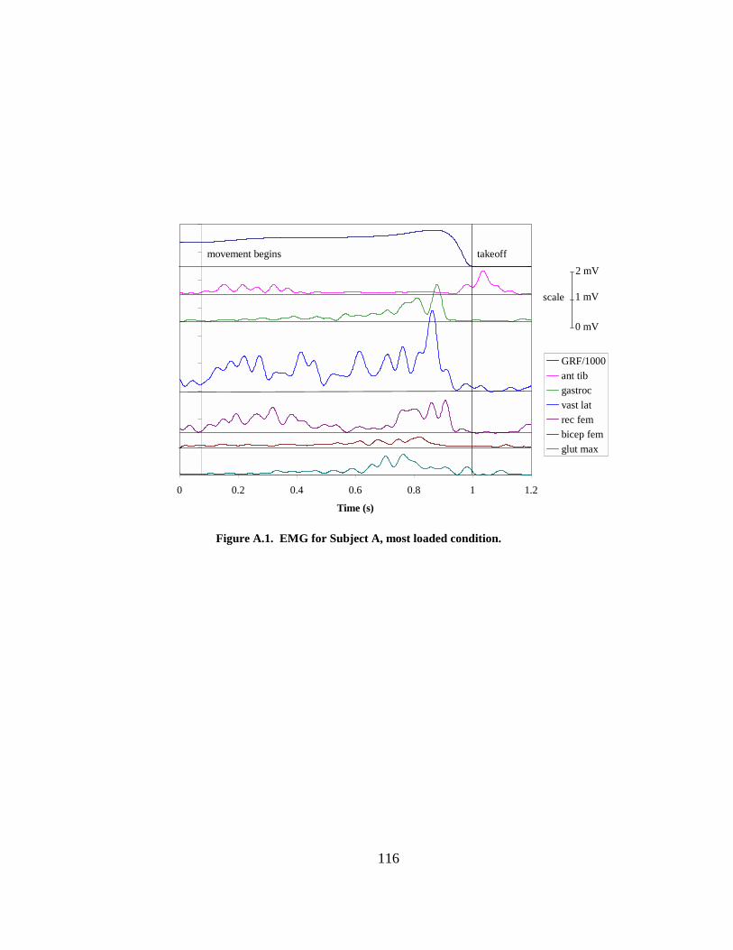
116
0 0.2 0.4 0.6 0.8 1 1.2
Time (s)
GRF/1000ant tibgastrocvast latrec fembicep femglut max
movement begins takeoff2 mV
1 mV
0 mV
scale
Figure A.1. EMG for Subject A, most loaded condition.
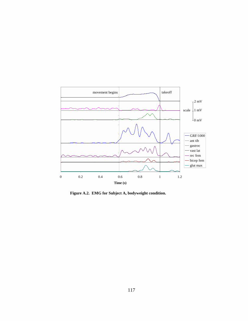
117
0 0.2 0.4 0.6 0.8 1 1.2
Time (s)
GRF/1000ant tibgastrocvast latrec fembicep femglut max
movement begins takeoff
2 mV
1 mV
0 mV
scale
Figure A.2. EMG for Subject A, bodyweight condition.
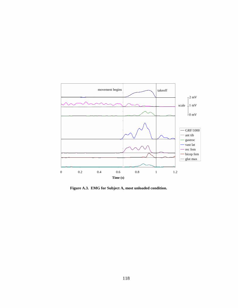
118
0 0.2 0.4 0.6 0.8 1 1.2
Time (s)
GRF/1000ant tibgastrocvast latrec fembicep femglut max
movement begins takeoff
2 mV
1 mV
0 mV
scale
Figure A.3. EMG for Subject A, most unloaded condition.
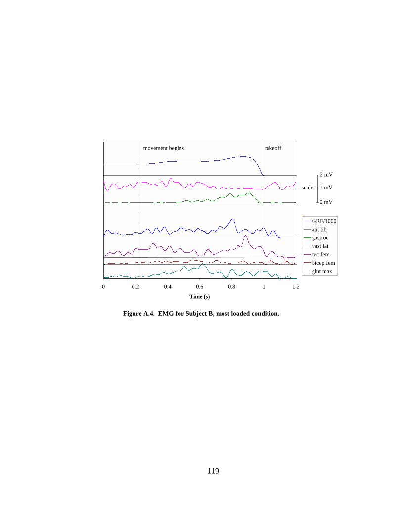
119
0 0.2 0.4 0.6 0.8 1 1.2
Time (s)
GRF/1000ant tibgastrocvast latrec fembicep femglut max
2 mV
1 mV
0 mV
scale
takeoffmovement begins
Figure A.4. EMG for Subject B, most loaded condition.
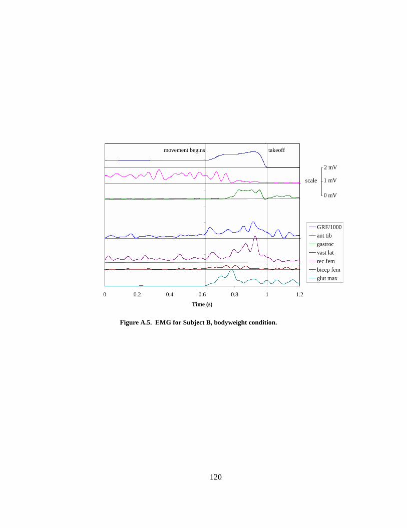
120
0 0.2 0.4 0.6 0.8 1 1.2
Time (s)
GRF/1000ant tibgastrocvast latrec fembicep femglut max
2 mV
1 mV
0 mV
scale
takeoffmovement begins
Figure A.5. EMG for Subject B, bodyweight condition.
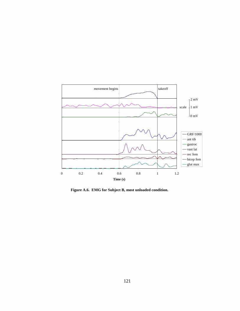
121
0 0.2 0.4 0.6 0.8 1 1.2
Time (s)
GRF/1000ant tibgastrocvast latrec fembicep femglut max
2 mV
1 mV
0 mV
scale
takeoffmovement begins
Figure A.6. EMG for Subject B, most unloaded condition.
122
Appendix B. Results of Pilot Studies
123
This appendix explains the pilot studies that were undertaken to determine the
best solution to unload the subjects to produce higher center of mass velocities. This was
not a simple problem; the requirements were that the subject should be assisted in the
movement by a vertical force that was as constant as possible to mirror the loaded
conditions.
Original Apparatus
The first attempt to build an assisting apparatus utilized a block and tackle system,
with a mechanical advantage of three, to produce a counterweight in the unloaded trials.
A stack of weights was attached to one side of the pulley system, and the subject in the
harness was attached to the opposite side. The idea was to put the mechanical advantage
of the pulley system on the side of the subject. This meant that the counterweight, which
would have the maximum potential to fall with the acceleration of gravity, would only
have to accelerate at one third of the acceleration of the subject. Since the subjects could
not accelerate at a rate greater than three times gravity, there would always be an
assisting force pulling on the subject as they jumped.
In fact, the mechanism worked. There was no slack in the rope as the subjects
jumped (as determined by video analysis), indicating that there was always a pulling
force on the subject. However, an analysis of the force readings from the transducer
connected to the harness the subjects were wearing indicated that there was a decrease in
force that went nearly to zero. Because the force did not drop completely to zero meant
that there was still tension in the rope, but the effectiveness of the counterweight was lost
nearly completely. There was almost no change in the maximum velocity during the
unloaded jumps using this method. The inertia of the counterweight and the friction of
the pulley system were believed to be the cause of the decrease in force during the jumps.
Regardless, the system did not meet the experimental requirements and was rejected.
Current Apparatus
The velocity vs. time profile for one subject attained with the current apparatus
utilizing filled elastic surgical tubing for the unloading mechanism was nearly the same
as Figure 4.1. When the data from the loaded, bodyweight, and unloaded trials were
combined, a wide range of peak velocities was produced. Two subjects were tested using
124
a protocol similar to the one presented in the Methods. The results of both subjects
indicated that a range of peak velocities both higher and lower than a normal jump was
attainable using the current apparatus. The force record from the transducer connected to
the harness indicated that the force decreased up to about 25% as the subject jumped due
to the elastic properties of the bands. However, the force difference was apparently small
enough to produce changes in peak velocity of the center of mass between the conditions.
Three trials at each condition were performed. The trial to trial differences in the
same condition for each subject were small. Therefore, to reduce data analysis time, only
the trial with the highest peak velocity was chosen for the main experiment. The ground
reaction force vs. maximum center of mass and the power vs. maximum center of mass
plots showed the general trends expected for the experiment. Therefore, it was concluded
that the apparatus and protocol were satisfactory to investigate force-velocity
relationships in the vertical jump.
125
Appendix C. Informed Consent Form
126
Informed Consent Form The Pennsylvania State University
Title of Project: Power and Force Production in the Vertical Jump with Varying Load Principal Investigator: Vladimir Zatsiorsky, Ph.D. Other Investigators: Andrew Hardyk, M.S. This is to certify that I, , have been given the following information with respect to my participation as a volunteer in a program of investigation supervised by Dr. Zatsiorsky.
1. Purpose of the Study: The purpose of this study is to examine the muscular power and force production in humans at various jumping velocities in the vertical jump.
2. Procedures to be Followed:
You will be asked to perform several vertical jumps from a stationary position. Three types of loading conditions will take place: no load, unloaded, and loaded. In the no load condition, you will place your hands on the broomstick that is provided and jump straight up without a countermovement (i.e. you will start from a lowered position and jump upward without first moving downward). In the loaded condition, you will hold a barbell with weights on your shoulders (similar to the squat in weight lifting) and jump upward. A special apparatus will take the weight away while you are in the air to protect you when you land. In the unloaded condition, you will be attached to a harness which will make you lighter. Once again, you will place your hands on the broomstick and jump straight upward. All of these jumps should be maximal attempts for maximum height. EMG electrodes will be attached to your skin on your leg muscles to record the activity of your muscles during the jumps. You will also be videotaped to determine the positions of your body during the movements.
3. Discomforts and Risks
In the loaded condition, there is the possibility that you will perceive discomfort because of the weight on your shoulders. The bar has been padded to alleviate this discomfort. You will also be instructed in the proper technique to use, and you will be required to use a weight belt to protect your lower back from any potential injury. There is also a possibility that the barbell could come in contact with your body after it is taken from you in midflight. Once again, the padding on the barbell will prevent any serious problems. Upon removal, the EMG electrodes may
127
cause some slight skin irritation. Appropriate clean up materials will be provided to you which should alleviate any discomfort.
4. a. Benefits to You:
You will receive no direct benefits such as financial compensation or class credit for your participation in this study.
b. Potential Benefits to Society:
Society could potentially benefit from a greater understanding of power production in human movements. This could manifest itself in the area of sports performance or in everyday life in such movements as rising from a chair.
5. Time Duration:
This study will require approximately two hours of your time.
6. Statement of Confidentiality: Your participation in this research is confidential. Only the investigators and his assistants will have access to your identity and to information that can be associated with your identity. In the event of publication of this research, no personally identifying information will be disclosed.
7. Right to Ask Questions:
You have the right to ask questions at any time before, during, or after the study. If you have questions in the future, please contact either: Andrew Hardyk Vladimir Zatsiorsky 200 Biomechanics Lab 200 Biomechanics Lab University Park, PA 16802 University Park, PA 16802 (814) 865-3445 (814) 865-3445 I have been given an opportunity to ask any questions I may have, and all such questions have been answered to my satisfaction.
8. Compensation
I understand that in the event of injury resulting from research, neither financial compensation nor free medical treatment is provided for such injury by the University. Questions regarding this statement or your rights as a subject of this research should be directed to the Office for Regulatory Compliance in 212 Kern Building, University Park, PA (814-865-1775).
9. Voluntary Participation:
I understand that my participation in this study is voluntary, and that I may withdraw from this study at any time by notifying the investigator. My
128
withdrawal from this study or my refusal to participate will in no way reflect my care or access to medical services.
This is to certify that I consent to and give permission for my participation as a volunteer in this program of investigation. I understand that I will receive a signed copy of this consent form. I have read this form and understand the content of this consent form.
Volunteer Date
I, the undersigned, have defined and explained the studies involved to the above volunteer. Investigator Date
Vita
Andrew Timothy Todd Hardyk Andrew Hardyk is wrapping up his career as a professional student and plans to
spend more time on the job that actually pays the bills. He is currently an Assistant Track
and Field Coach at Penn State University and hopes to incorporate his research skills in
developing better coaching techniques to develop the next generation of track and field
superstars. He sees a huge divide between scientists and coaches and sincerely hopes that
he can help to bridge that gap by working from both sides.
Hardyk graduated from the University of Cincinnati in 1992 with a Bachelor of
Science degree in Aerospace Engineering and a Master of Science in Engineering
Mechanics one year later, specializing in orthopedic biomechanics. At Cincinnati, he
was a team co-captain for the track and field team and received the ‘Jimmy Nippert
Award’ for the most outstanding all-around senior male athlete. Post-collegiately, he
competed in the United States Track and Field Championships four times, twice in the
long jump and twice in the 100m and was selected to represent the North team at the U.S.
Olympic festival in 1995. In five years as a coach at Penn State, he has produced 10 All-
Americans and has had numerous NCAA qualifiers.
Hardyk currently has limited publications to his name, but hopes that this
dissertation will be a source for several in the near future. He gave a presentation in 1994
at the American Society of Biomechanics Annual Meeting entitled, “Strategies Used By
Elite Male Gymnasts to Generate High Forward Angular Momentum During Takeoff in
Vaulting: A Cluster Analysis,” and was a co-author of a chapter on sprint training
entitled, “Sport Speed,” that was published earlier this year.
Hardyk is very happily married to the former Angela Showalter, who is an
Obstetrics and Gynecology resident at the Penn State/Hershey Medical Center.