Force distribution for a flat belt drive with a concentrated contact load

Mech. Mach. Theory Vol. 25, No. 6. pp. 667-677. 1990 0094-114X/90 $3.00 + 0.00 Printed in Great Britain. All rights reserved Copyright ~ 1990 Pergamon Press plc

F O R C E D I S T R I B U T I O N F O R A F L A T B E L T D R I V E

W I T H A C O N C E N T R A T E D C O N T A C T L O A D

HYUNSOO KIM Department of Mechanical Engineering, Sungkyunkwan University, Suwon City, 440-746 S. Korea

KURT M. MARSHEK Department of Mechanical Engineering, The University of Texas at Austin, Austin, TX 78712, U,S.A.

(Received 16 June 1989; /n revised form 10 August 1989; received for publication 28 November 1989)

Abstract--An equation based on the classical Euler formula is derived to investigate the normal and tangential belt force distribution of a flat belt drive when a concentrated contact load is applied on the pulley. This loading condition occurs in an abrasive belt grinding. The belt force equation presented in this paper has a constant coefficient of friction. Analytical results show good agreement with the experimental results and the authors' previous work, which is based on a surface model of the belt friction face with a varying coefficient of friction. The equation developed from the Euler formula is suggested for practical design due to its sufficient accuracy and simplicity.

1. INTRODUCTION

In flat belt drives with concentrated contact load on the pulley, such as in abrasive belt grinding, contact occurs on both sides of the belt: (1) inside contact between the pulley and the belt and (2) outside contact between the belt and the workpiece (a concentrated contact load). The outside contact makes the belt drive more complicated and results in a different belt force distribution compared with those of the ordinary fiat belt drive.

Namba and Tsuwa [1, 2] measured a pressure distribution for the concentrated contact area in an abrasive belt grinding and suggested a formula for the contact length including an effect of the belt. Kim et al. [3] obtained a belt force distribution for a grinding belt drive without the concentrated contact load and suggested a surface model for the belt friction. According to Kim et al. [3], the coefficient of friction changes as a function of pressure and the surface model constant. Kim and Marshek [4, 5] also measured the belt force distribution for the entire arc of contact between the belt and pulley with concentrated contact load and compared the experimental results with theoretical results based on the surface model.

In this paper, the distribution of normal and tangential belt forces with concentrated contact load is obtained based on the classical Euler formula with a constant coefficient of friction. Analytical results are compared with those obtained from an experiment and the previous work [4] that was performed with a varying coefficient of friction of the surface model.

2. THEORETICAL ANALYSIS

2.1. Driven pu l ley contac t

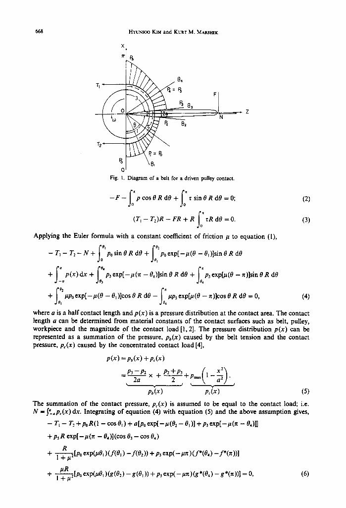
Figure 1 shows a free body diagram of a belt in a quasi-static equilibrium state on a driven pulley. The entire arc of contact can be divided into three areas: (1) entry point to (concentrated) contact area; (2) contact area and (3) contact area to exit point. The areas (1) and (3) are divided into inactive and active regions for the applied torque load. In the inactive region, there is only a static friction between the belt and the pulley. In the active region, kinetic friction occurs because of belt slip, and this friction causes belt tension to change.

From quasi-static equilibrium requirement, Fig. 1, the following equations are obtained:

f: fo - T~ - T2 - N + p sin O R dO + z cos O R dO = O; (1)

MMr .,~ ~F 667

668 HYUNSOO KtM and KLx'r M. Mm, srmK

X

T I =

F

~, ,.Q • 2 -

Tz" p , = ~ \

F i g . 1. Diagram of a belt for a driven pulley contact.

, , - ~ 7

N

- F - f~pcosO R dO + f~ ~ sinO R dO =O; (2)

(T~ - T2)R - FR + R ~ rR dO = O. (3)

Applying the Euler formula with a constant coefficient of friction/z to equation (1),

fo f; - Ti -- T 2 - N + posinOR d0 + p0 e x p [ - ~ ( 0 --Oi)]sinOR dO !

f , . f : + p ( x ) d x + P5 e x p [ - ~ ( ~ - 04)]sin 0 R d0 + P5 exp[~(0 - :0]sin 0 R d0

a . ] 0 3 4

I; I: + ~P0 e x p [ - g (0 - 01 )lcos 0 R d0 - ~P5 exp[~ (0 - n)lcos 0 R d0 = 0, (4) ! 4

where a is a half contact length and p(x) is a pressure distribution at the contact area. The contact length a can be determined from material constants o f the contact surfaces such as belt, pulley, workpiece and the magnitude of the contact load [1, 2]. The pressure distribution p(x) can be represented as a summation of the pressure, pb(x) caused by the belt tension and the contact pressure, pc(x) caused by the concentrated contact load [4],

p(x) = p~(x) + pAx)

_ _ P3 P2 × + P 2 ~ _ + P3 b P m a x 1 - .

2a 2 k I ~, I

v Y

pb(x) pc(x) (5)

The summation of the contact pressure, pc(x) is assumed to be equal to the contact load; i.e. N = S~apc(x) dx. Integrating of equation (4) with equation (5) and the above assumption gives,

- - Ti -- 7'2 + Po R (1 - cos 01 ) + a [Po exp[ - / z (02 - 01 )] + P5 exp[ - g (~ -- 04)]]

+Psg exp[--#(~ -- 04)](cos 03 - cos 04)

R + l - - ~ 2 [ p o expOaO, )(f(O, ) - f ( 0 2 ) ) + P5 exp(- /a : t ) (f*(04) - f * ( = ) ) ]

+ ~ [ P o exp(/~0, )(g(02) - g(O, )) + P5 e x p ( - / ~ ) (g*(04) - g*(~))] = 0, (6) | -t-/~-

Force distribution for a fiat belt drive 669

where

f(O) = exp(/~0)(cos 0 + # sin 0),

g(O) = exp(-#0)(s in 0) - # cos 0),

i f ( 0 ) = exp(#0)(cos 0 - /~ cos 0),

g*(O) = exp(#0)(sin 0 + # cos 0).

In order to integrate equations (2) and (3), the distribution of tangential friction force S'-= ~(x) dx should be obtained. The friction force can be calculated from z =/~p with a constant coefficient of friction.

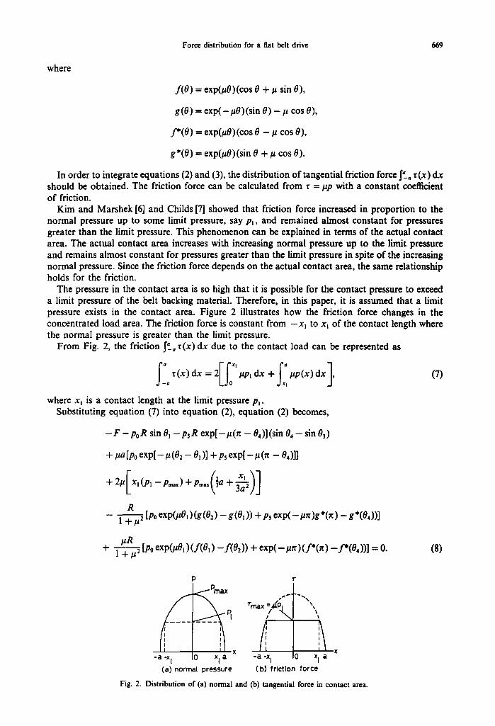
Kim and Marshek [6] and Childs [7] showed that friction force increased in proportion to the normal pressure up to some limit pressure, say Pt, and remained almost constant for pressures greater than the limit pressure. This phenomenon can be explained in terms of the actual contact area. The actual contact area increases with increasing normal pressure up to the limit pressure and remains almost constant for pressures greater than the limit pressure in spite of the increasing normal pressure. Since the friction force depends on the actual contact area, the same relationship holds for the friction.

The pressure in the contact area is so high that it is possible for the contact pressure to exceed a limit pressure of the belt backing material. Therefore, in this paper, it is assumed that a limit pressure exists in the contact area. Figure 2 illustrates how the friction force changes in the concentrated load area. The friction force is constant from -xm to xl of the contact length where the normal pressure is greater than the limit pressure.

From Fig. 2, the friction S=__o ~(x)dx due to the contact load can be represented as

=2[fo'.ptdx + fxi (7)

where xj is a contact length at the limit pressure p,. Substituting equation (7) into equation (2), equation (2) becomes,

- F -poR sin Oi -psR e x p [ - # ( n - 04)](sin O, - sin 03)

+ pa[po e x p [ - - /t (02 - - Ot )] + P5 e x p [ - # ( n - 04)]]

R 1 + U 2 [P0 exp~0m ) (g(02) - g(O, )) +Ps e x p ( - #Tt)g*(Tr) - g*(0,))]

+ ~ [P0 exp~0t ) (f(O,) -f(02 )) + exp( - #tr ) (f*(n) -if(O,))] = 0. (8)

P

I

I I I X - a -x I 0 x I a

(a) normal p ressu re

o S ~ ".*%.

I

I :

- a -x I 0 x I a

( b ) f r i c t i on f o r c e

Fig. 2. Distribution of (a) normal and (b) tangential force in contact area.

670 Hvussoo KIM and KURT M. MAgSHEK

Similarly, equation (3) becomes,

p0R[1 - exp[-#(02 - 0, )]] + #a[po e x p [ - # ( 0 , - 0, )] + Ps e x p [ - # ( ~ - 04)]]

+ 2 # x,(p,--Pmax)+Pma~ ~a + 3a2jj--p,R[l--exp[--#(~--04)l]=O. (9)

If the limit pressure p~ is lower than the maximum pressure Pma~, the above equations can be used simply by substituting pl = Pmax.

With known data, the concentrated contact load N and the friction force F obtained from experiments, the three unknowns 01, 04 and p~ can be determined by numerical iteration of equations (6), (8) and (9). Solving equations (6), (8) and (9) gives the value of the limit pressure p~ and the normal and tangential belt force distribution along the entire arc of contact between the belt and the pulley.

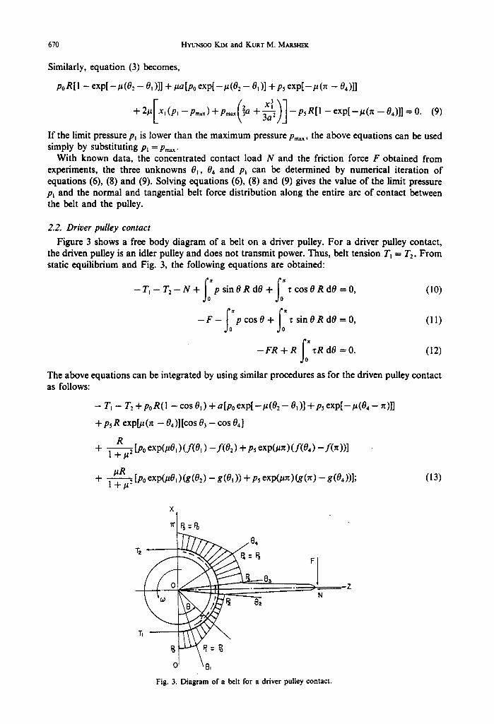
2.2. Driver pulley contact Figure 3 shows a free body diagram of a belt on a driver pulley. For a driver pulley contact,

the driven pulley is an idler pulley and does not transmit power. Thus, belt tension Tt = T2. From static equilibrium and Fig. 3, the following equations are obtained:

- T , - T 2 - N + f : p sinO R dO + f: 'r cosO R dO =O, (10)

-F-f:pcosO+ f: sinORdO=O, (11)

- F R + R f~ "oR dO = O. (12)

The above equations can be integrated by using similar procedures as for the driven pulley contact as follows:

- Ti - 7"2 + p0R(l - cos 0, ) + a[po e x p [ - - # ( 0 2 -- 0m )] + P5 exp[ -#(04 - 7t)]]

+ P5 R expLu 0t - 04)] [cos 03 - cos 04]

R + ~ [Po exp(#O, ) (f(O,) -f(02 ) + P5 exp~rt ) (f(O,) - f O r ))]

+ ~ [P0 exp(#0, )(g(O2) - g(O, )) + p~ exp(#n) (g(lr) - g(04))]; (I 3)

~ , 84 F ]

" r~ '~ "~'~ ~ '~2 o ) r ~ ~N ,,Z

1"ITI ~Pi --Po

O' "t3~ Fig. 3. Diagram of a belt for a driver pulley contact.

Force distribution for a fiat belt drive 671

-F -poR sin Oj -psR exp~ (Tr - 8,)] (sin 04 - sin 83)

+ ~ [Po exp[-/a (02 - 0~ )] + p~ exp[-/a (8, - ~)]]

+ 2 / ~ [ x , ( p , - p ~ ) + p ~ (Z3a + ~a2,/jx2"]

R 1 + p2 [Po exp(p01) (g(02) - g(01 )) + P5 exp(/zn) (g(Tt) -- g(04))]

/zR + ~ [Po exp0a0, )(f(O, ) -f(02)) + p, exp0alt)(f(O,) - f (~) ) ] = 0; (14)

- F + [Po R (1 - exp[-/a (02 - 0~ )]] +/aa [Po exp[-/a (02 - 0~ )] + P5 exp[-/z (04 - 0~)]] •

+2/~ , (p , -p .~)+p~.~ ~a +y-~a2/.] p,R[exp~(n -0,)]- 11=0. (15)

3. E X P E R I M E N T

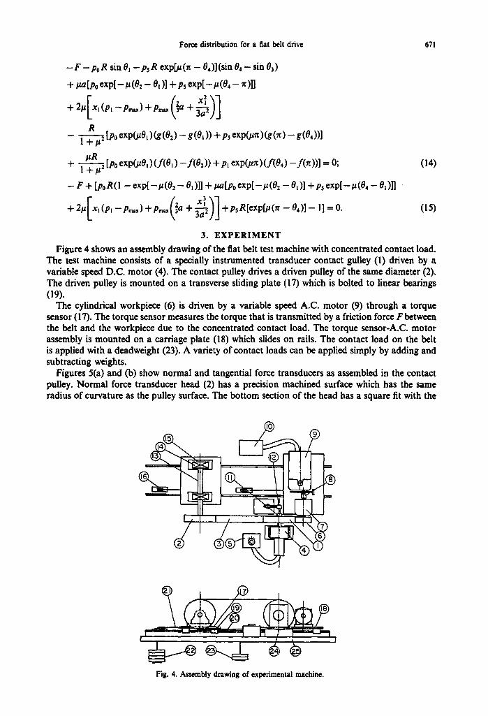
Figure 4 shows an assembly drawing of the fiat belt test machine with concentrated contact load. The test machine consists of a specially instrumented transducer contact gulley (1) driven by a variable speed D.C. motor (4). The contact pulley drives a driven pulley of the same diameter (2). The driven pulley is mounted on a transverse sliding plate (17) which is bolted to linear bearings (19).

The cylindrical workpiece (6) is driven by a variable speed A.C. motor (9) through a torque sensor (17). The torque sensor measures the torque that is transmitted by a friction force F between the belt and the workpiece due to the concentrated contact load. The torque sensor-A.C, motor assembly is mounted on a carnage plate (18) which slides on rails. The contact load on the belt is applied with a deadweight (23). A variety of contact loads can be applied simply by adding and subtracting weights.

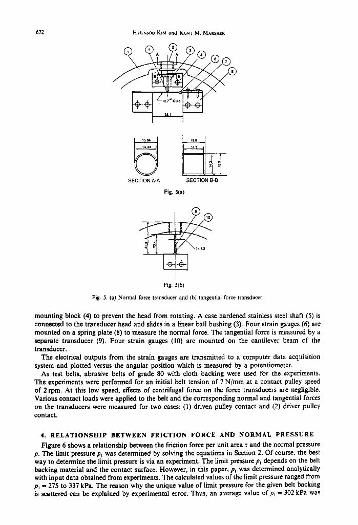
Figures 5(a) and (b) show normal and tangential force transducers as assembled in the contact pulley. Normal force transducer head (2) has a precision machined surface which has the same radius of curvature as the pulley surface. The bottom section of the head has a square fit with the

s[ ~.,

= = " . . . . . . . I " 9

Fig. 4. Assembly drawing of experimental machine.

672 HYUNSOO KIM and KURT M. MARSHEK

111 I

/12.7 w X 0

38J

®

CJ SECTION A-A

14.3

Z

SECTION B-B

Fig. 5(a)

[÷ Fig. 5(b)

Fig. 5. (a) Normal force transducer and (b) tangential force transducer.

mounting block (4) to prevent the head from rotating. A case hardened stainless steel shaft (5) is connected to the transducer head and slides in a linear ball bushing (3). Four strain gauges (6) are mounted on a spring plate (8) to measure the normal force. The tangential force is measured by a separate transducer (9). Four strain gauges (10) are mounted on the cantilever beam of the transducer.

The electrical outputs from the strain gauges are transmitted to a computer data acquisition system and plotted versus the angular position which is measured by a potentiometer.

As test belts, abrasive belts of grade 80 with cloth backing were used for the experiments. The experiments were performed for an initial belt tension of 7 N/ram at a contact pulley speed of 2 rpm. At this low speed, effects of centrifugal force on the force transducers are negligible. Various contact loads were applied to the belt and the corresponding normal and tangential forces on the transducers were measured for two cases: (l) driven pulley contact and (2) driver pulley contact.

4. RELATIONSHIP BETWEEN FRICTION FORCE AND NORMAL PRESSURE

Figure 6 shows a relationship between the friction force per unit area ~ and the normal pressure p. The limit pressure pl was determined by solving the equations in Section 2. Of course, the best way to determine the limit pressure is via an experiment. The limit pressure Pi depends on the belt backing material and the contact surface. However, in this paper, pl was determined analytically with input data obtained from experiments. The calculated values of the limit pressure ranged from Pl = 275 to 337 kPa. The reason why the unique value of limit pressure for the given belt backing is scattered can be explained by experimental error. Thus, an average value of p~ = 302 kPa was

Force distribution for a flat belt drive 673

kPa 80

60 Euler / ~

_ _

2 '- 40 .9 ~ = t .

~- 20

, , F ~ , j , , 0 100 200 300 400 500 600 kPa

normal pressure

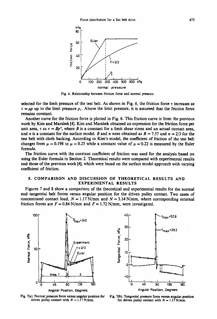
Fig. 6. Relationship between friction force and normal pressure.

selected for the limit pressure of the test belt. As shown in Fig. 6, the friction force z increases as =/~p up to the limit pressure pl. Above the limit pressure, it is assumed that the friction force

remains constant. Another curve for the friction force is plotted in Fig. 6. This friction curve is from the previous

work by Kim and Marshek [4]. Kim and Marshek obtained an expression for the friction force per unit area, ~ as ¢ = Bp', where B is a constant for a limit shear stress and an actual contact area, and n is a constant for the surface model. B and n were obtained as B -- 7.57 and n --- 2/3 for the test belt with cloth backing. According to Kim's model, the coefficient of friction o f the test belt changes from # = 0.198 to/~ = 0.25 while a constant value of/~ = 0.22 is measured by the Euler formula.

The friction curve with the constant coefficient of friction was used for the analysis based on using the Euler formula in Section 2. Theoretical results were compared with experimental results and those of the previous work [4], which were based on the surface model approach with varying coefficient of friction.

5. C O M P A R I S O N A N D D I S C U S S I O N O F T H E O R E T I C A L R E S U L T S A N D E X P E R I M E N T A L R E S U L T S

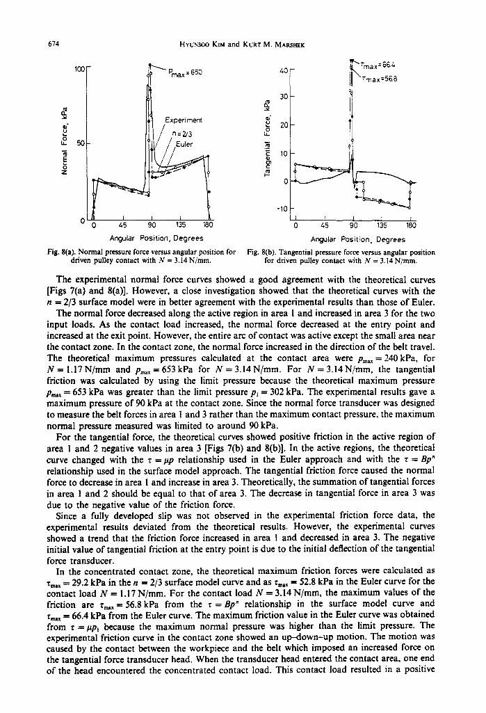
Figures 7 and 8 s h o w a c o m p a r i s o n o f the theoretical and experimental results for the normal and tangential belt forces versus angular pos i t ion for the d r i v e n pu l l ey contact . T w o cases o f concentrated contac t load, N = 1.17 N / m m and N = 3 . 1 4 N / m m , where corresponding external friction forces are F = 0.84 N / r a m and F = 1.72 N / r a m , were investigated.

.1°° I i~ Pr~x =2~o ~. ~,ll Experiment

50 n = 2/3

Z •

o ! - : f 0 45 90 135 180

Angular Position, Degrees

Fig. 7(a). Normal pressure force versus angular position for driven pulley contact with N = 1.17 N/mm.

=- u

t L

e -

e "

40

30

20

10

-10

~'max =52.8

m'rmax = 29.2

I t I ! ]

0 45 90 135 180

Angular Position. Degrees

Fig. 7(b). Tangential pressure force versus angular position for driven pulley contact with N = I.I? N/mm.

674 HYUN$OO KIM a n d KURT M. MARSI.~K

100- ~ " " Pmax = 650

I,I,I E x p e r i m e n t

~ so

Z

0 45 90 135 180


Fig. 8(a). Normal pressure force versus angular position for driven pulley contact with N = 3.14 N/ram.

z.0

30

u 20

E I0 ~a o i

0

-10 I I : I

0 45 90 135 180


Fig. 8(b). Tangential pressure force versus angular position for driven pulley contact with N = 3.14 N/ram.

The experimental normal force curves showed a good agreement with the theoretical curves [Figs 7(a) and 8(a)]. However, a close investigation showed that the theoretical curves with the n = 2/3 surface model were in better agreement with the experimental results than those o f Euler.

The normal force decreased along the active region in area 1 and increased in area 3 for the two input loads. As the contact load increased, the normal force decreased at the entry point and increased at the exit point. However, the entire arc of contact was active except the small area near the contact zone. In the contact zone, the normal force increased in the direction of the belt travel. The theoretical maximum pressures calculated at the contact area were Pma~ = 240 kPa, for N = 1.17N/mm and Pma, = 653 kPa for N = 3.14N/mm. For N = 3.14N/mm, the tangential friction was calculated by using the limit pressure because the theoretical maximum pressure Pm,x = 653 kPa was greater than the limit pressure pl = 302 kPa. The experimental results gave a maximum pressure of 90 kPa at the contact zone. Since the normal force transducer was designed to measure the belt forces in area I and 3 rather than the maximum contact pressure, the maximum normal pressure measured was limited to around 90 kPa.

For the tangential force, the theoretical curves showed positive friction in the active region of area 1 and 2 negative values in area 3 [Figs 7(b) and 8(b)]. In the active regions, the theoretical curve changed with the ~ = #p relationship used in the Euler approach and with the T = Bp" relationship used in the surface model approach. The tangential friction force caused the normal force to decrease in area 1 and increase in area 3. Theoretically, the summation of tangential forces in area 1 and 2 should be equal to that of area 3. The decrease in tangential force in area 3 was due to the negative value of the friction force.

Since a fully developed slip was not observed in the experimental friction force data, the experimental results deviated from the theoretical results. However, the experimental curves showed a trend that the friction force increased in area 1 and decreased in area 3. The negative initial value of tangential friction at the entry point is due to the initial deflection of the tangential force transducer.

In the concentrated contact zone, the theoretical maximum friction forces were calculated as ~m~ = 29.2 kPa in the n = 2/3 surface model curve and as ~m,, = 52.8 kPa in the Euler curve for the contact load N = 1.17 N/mm. For the contact load N = 3.14 N/mm, the maximum values of the friction are ~m~ = 56.8 kPa from the T = Bp" relationship in the surface model curve and ~m,~ = 66.4 kPa from the Euler curve. The maximum friction value in the Euler curve was obtained from ~---/~Pl because the maximum normal pressure was higher than the limit pressure. The experimental friction curve in the contact zone showed an up--clown-up motion. The motion was caused by the contact between the workpiece and the belt which imposed an increased force on the tangential force transducer head. When the transducer head entered the contact area, one end of the head encountered the concentrated contact load. This contact load resulted in a positive


i X Prnax= 2/-.0 Ioo I ~ ~,o -

3O

u /Experiment t~ 2C

n:2 /3

-i d -10 0 i J I I I

0 45 90 135 180 0 45 90

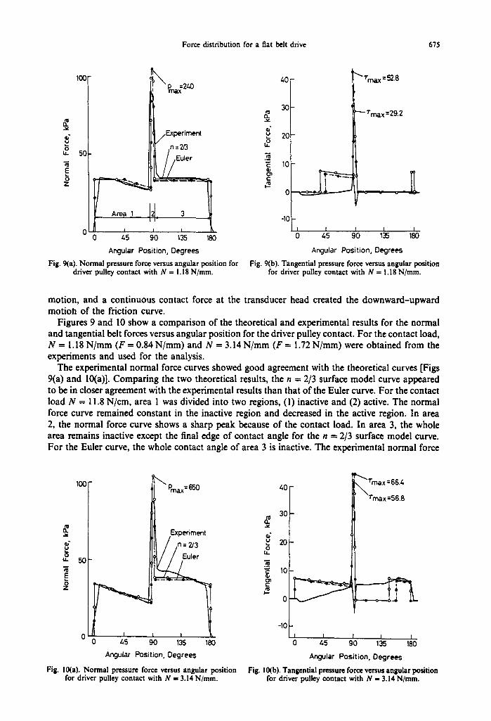
Angular Position, Degrees Fig. 9(a). Normal pressure force versus angular position for

driver pulley contact with N = 1.18 N/tara.

b ¢ m a x :52.8

~ ' - Tma x =29.2

I I 135 180


Fig. 9(b). Tangential pressure force versus angular position for driver pulley contact with N -- 1.18 N/ram.

motion, and a continuous contact force at the transducer head created the downward-upward motioh of the friction curve.

Figures 9 and 10 show a comparison of the theoretical and experimental results for the normal and tangential belt forces versus angular position for the driver pulley contact. For the contact load, N = 1.18 N/mm (F = 0.84 N/mm) and N = 3.14 N/mm (F = 1.72 N/mm) were obtained from the experiments and used for the analysis.

The experimental normal force curves showed good agreement with the theoretical curves [Figs 9(a) and 10(a)]. Comparing the two theoretical results, the n = 2/3 surface model curve appeared to be in closer agreement with the experimental results than that of the Euler curve. For .the contact load N = 11.8 N/cm, area 1 was divided into two regions, (1) inactive and (2) active. The normal force curve remained constant in the inactive region and decreased in the active region. In area 2, the normal force curve shows a sharp peak because of the contact load. In area 3, the whole area remains inactive except the final edge of contact angle for the n = 2/3 surface model curve. For the Euler curve, the whole contact angle of area 3 is inactive. The experimental normal force

I IIII Experiment n : 2 / 3

O u. 50 ¢¢

0 L[= I I I k 0 45 90 135 180


Fig. 10(a). Normal pressure force versus angular position for driver pulley contact with N = 3.14 N/tara.

u

O~ t -

40

30

20

10

0 45 90 135 180


Fig. 10(b). Tangential pressure force versus angular position for driver pulley contact with N ffi 3.14 N/tara.

676 HYUNSOO KtM and KugT M. MARSHEK

curve remains constant along the contact arc except for the final 15 degrees of contact angle where the force decreases. As the contact load increased, area 1 became active first and the active region in area 3 extended backwards towards the contact zone [Fig. 10(a)].

For the tangential force curves [Figs 9(b) and 10(b)], the theoretical tangential force occurred in the active region of area 1 and 3 according to the ~ =/~p relationship in the Euler curve and z = Bp" in the surface model curve. The friction force caused the normal force to decrease. For the experimental force curves, the friction force increased slightly in the active region of area 1 and remained constant in area 3 for N = !.18 N/mm.

As the contact load increased, the experimental friction force increased in the active region of area 1 and 3. However, the value of the friction force was lower than the theoretical values. This can be explained by a partially developed slip measured through the tangential force transducer [3, 4]. Once a fully developed slip occurred, the experimental curve followed the theoretical curve, which can be seen for the final 20 degrees of the contact area 3 for N = 3.14 N/mm [Fig. 10(b)].

Comparing the experimental results with two theoretical results of: (1) the surface model approach and (2) the Euler formula, the surface model method gave better results than those for the Euler formula. However, the surface model approach requires experiments to obtain the constants, B and n [3]. The Euler formula predicted the belt force distribution with sufficient accuracy. Since the Euler formula uses a constant coefficient of friction and it is simple to determine the coefficient of friction by experiment, it is suggested that the Euler formula be used for practical design. However, in using the Euler formula for the flat belt drive with concentrated contact load, the value o f limit pressure should be determined in the contact area where high normal pressure exists. Even if the value of limit pressure was determined analytically in this paper, it is the best to obtain the limit pressure experimentally. It will be interesting future work to determine the value of limit pressure for various belt backing materials by experiments.

6. C O N C L U S I O N S

I. For the driven pulley contact, the entire arc of contact was active except for the small area near the contact zone in area 3 (from the contact zone to the exit point) regardless of the magnitude of the contact load in the experimental range. The tangential force in the active region of area 1 (from the entry point to the contact zone) was in the direction of rotation of the contact pulley and caused the normal force to decrease. In area 3, the tangential friction force was in a direction opposite to the direction of the friction of area 1 and caused the normal force to increase.

2. For the driver pulley contact, each area of 1 and 3 was divided into (1) inactive and (2) active regions. As the contact load increased, area 1 was active first. In area 3, the active region extended towards the contact zone. The tangential friction force in the active area caused the normal force to decrease.

3. Analytical results showed close agreement with the experimental results for the belt normal forces. For the tangential friction force, direct comparison was difficult because of the partially developed slip on the belt surface. Although the surface model approach gave better results than the Euler formula, it is suggested that the Euler formula be used for practical design since it is relatively easier to apply rather than the surface model approach and gives sufficient accuracy.

REFERENCES

I. Y. Namba and H. Tsuwa, Tech Rep. Osaka Unit,. 20, 249 (1970). 2. Y. Namba and H. Tsuwa, J. Jap. Soc. Prec. Engr. 36, 478-483 (1970). 3. H. Kim, K. M. Marshek and M. Naji, Mech. Mach. Theory 22, 97-103 (1987). 4. H. Kim and K. M. Marshek, ASMF. J. Ind. I!0, 201-211 (1988). 5. K. M. Marshek and H. Kim, U. S. Patent No. 4,762,005, Aug. 9 (1988). 6. H. Kim and K. M. Marshek, A S M E J. Mech. Transm. Automn Des. 110, 93-99 (1988). 7. T. H. C. Childs. Int. J. Mech. Sci. 22, 117-126 (1980).


D I S T R I B U T I O N D E S F O R C E S P O U R U N E N T R A I N E M E N T A

C O U R R O I E P L A T E A V E C C H A R G E D E C O N T A C T C O N C E N T R E E

R6mm6----Une 6quation bas6e sur la formule classique d'Euler est d~riv6e pour rechercher la distribution des forces normales et tangentielles sur un entra~nement :i courroie plate quant une charge de contact concentr6e est appliqu6e sur la poulie. Cette condition de chargement appara~t lors du meulage avec courroie abrasive. L'6quation des forces pr6sent6e dans ce papier a un coefficient constant de friction. Les r6sultats analytiques sont en bon accord avec les r~sultats exp6rimentaux et le travail ant6rieur des auteurs, qui est bas6 sur un module de surface de la face de friction de la courroie utilisant un coefficient de friction variable. L'6quation d~velopp6e d partir de la formule d'Euler est proposde pour des applications pratiques grace :i sa pr6cision suffisante et sa simplicitd.

Documents

Force distribution for a flat belt drive with a concentrated contact load