Embed Size (px)
Citation preview
FORCE TRANSFER AROUND OPENINGS IN CLT SHEAR WALLS
by
Sai Ganesh Sarvotham Pai
B.Tech., National Institute of Technology, Karnataka, 2011
A THESIS SUBMITTED IN PARTIAL FULFILLMENT OF
THE REQUIREMENTS FOR THE DEGREE OF
MASTER OF APPLIED SCIENCE
in
THE FACULTY OF GRADUATE AND POSTDOCTORAL STUDIES
(Civil Engineering)
THE UNIVERSITY OF BRITISH COLUMBIA
(Vancouver)
December 2014
© Sai Ganesh Sarvotham Pai, 2014
ii
Abstract
During an earthquake, shear walls can experience damage around corners of doors and
windows due to development of stress concentration. Reinforcements provided to minimize
this damage are designed for forces that develop at these corners known as transfer forces. In
this thesis, the focus is on understanding the forces that develop around opening corners in
cross laminated timber (CLT) shear walls and reinforcement requirements for the same.
In the literature, four different analytical models are commonly considered to determine the
transfer force for design of wood-frame shear walls. These models have been reviewed in this
thesis. The Diekmann model is found to be the most suitable analytical model to determine the
transfer force around a window-type opening.
Numerical models are developed in ANSYS to analyse the forces around opening corners in
CLT shear walls. CLT shear walls with cut-out openings are analysed using a three-
dimensional brick element model and a frame model. These models highlight the increase in
shear and torsion around opening corners due to stress concentration. The coupled-panel
construction practice for CLT shear walls with openings is analysed using a continuum model
calibrated to experimental data. The analysis shows the increase in strength and stiffness of
walls, when tie-rods are used as reinforcement. Analysis results also indicate that the tie-rods
should be designed to behave linearly for optimum performance of the wall.
Finally, a linear regression model is developed to determine the stiffness of a simply-supported
CLT shear wall with a window-type opening. This model provides insight into the effect of
various geometrical and material parameters on the stiffness of the wall. The process of model

iii
development has been explained, which can be improved further to include the behaviour of
anchors.

iv
Preface
This dissertation is original, unpublished, independent work by the author, Sai Ganesh
Sarvotham Pai.

v
Table of Contents
Abstract .................................................................................................................................... ii
Preface ..................................................................................................................................... iv
Table of Contents .................................................................................................................... v
List of Tables .......................................................................................................................... ix
List of Figures .......................................................................................................................... x
Acknowledgements .............................................................................................................. xiv
Dedication .............................................................................................................................. xv
Chapter 1: Introduction ........................................................................................................ 1
1.1 Motivation ................................................................................................................. 1
1.2 Objectives ................................................................................................................. 2
1.3 Background ............................................................................................................... 2
1.4 Overview of the Thesis ............................................................................................. 8
Chapter 2: Analytical Models for Force Transfer around Openings ............................. 11
2.1 Drag Strut Analogy ................................................................................................. 11
2.2 Cantilever Beam Analogy ....................................................................................... 14
2.3 Coupled Beam Analogy .......................................................................................... 18
vi
2.4 Diekmann Method .................................................................................................. 24
2.5 Numerical Example ................................................................................................ 27
2.6 Finite Element Modeling and Comparison of Results ............................................ 33
2.7 Conclusions ............................................................................................................. 40
Chapter 3: CLT Shear Wall with a Cut-out Opening ...................................................... 41
3.1 In-plane Behaviour of CLT ..................................................................................... 41
3.2 CLT Shear Wall with a Cut-out Opening ............................................................... 47
3.3 Frame Model for a CLT Shear Wall with a Cut-out Opening ................................ 52
3.4 Results from the Frame Models (Model C) ............................................................ 56
3.5 Conclusions ............................................................................................................. 60
Chapter 4: Coupled-Panel CLT Shear Walls .................................................................... 62
4.1 Modeling a Coupled-Panel CLT Shear Wall .......................................................... 63
4.2 Modeling the CLT Panels ....................................................................................... 64
4.3 Connector Modeling ............................................................................................... 66
4.4 Contact Modeling.................................................................................................... 70
4.5 Displacement-based Pushover Analysis in ANSYS ............................................... 71
4.6 Modeling a Coupled Panel CLT Shear Wall with an Opening ............................... 74
vii
4.7 Pushover Analysis of a Coupled Panel CLT Shear Wall with an Opening ............ 76
4.8 Effect of Tie-Rods as Reinforcement on Performance of the CLT Shear Wall ..... 79
4.9 Effect of Anchoring and Opening Layout on Wall Behaviour ............................... 80
4.10 Design Transfer Force from the Diekmann Model and Finite Element Models .... 82
4.11 Effect of Tie-Rod Stiffness on Performance of the CLT Shear Wall ..................... 85
4.12 Conclusions ............................................................................................................. 87
Chapter 5: Linear Regression Model for Stiffness of a Wall ........................................... 89
5.1 General Form of a Linear Regression Model ......................................................... 89
5.2 Model Development................................................................................................ 92
5.3 Model Reduction ..................................................................................................... 97
Chapter 6: Conclusion and Future Work ........................................................................ 107
6.1 Conclusion ............................................................................................................ 107
6.2 Future Work .......................................................................................................... 108
References ............................................................................................................................ 109
Appendices ........................................................................................................................... 113
Appendix A Linear Regression Model for Stiffness of a CLT Shear Wall ...................... 113
A.1 Trials ................................................................................................................. 113

viii
A.2 Model Development Calculations..................................................................... 118

ix
List of Tables
Table 2.1 Transfer force from the finite element model ...................................................... 36
Table 3.1 Material property of CLT panel (Yawalata and Lam 2011) ................................ 49
Table 3.2 Comparison of stress in the glued surface ........................................................... 60
Table 4.1 Homogenized material property of a CLT panel ................................................. 65
Table 5.1 Input parameters of the finite element model ...................................................... 94
Table 5.2 Model parameters ................................................................................................ 96
Table 5.3 Model parameters of the regression model ........................................................ 102
Table 5.4 Model parameters of the reduced regression model .......................................... 105
x
List of Figures
Figure 1.1 Overview of finite element models ...................................................................... 8
Figure 2.1 Drag strut analogy .............................................................................................. 12
Figure 2.2 Cantilevered beam analogy ................................................................................. 15
Figure 2.3 Analysis of the full-width panel on the left side of the opening ........................ 16
Figure 2.4 Coupled beam analogy ....................................................................................... 19
Figure 2.5 Free-body diagram for coupled beam analogy ................................................... 22
Figure 2.6 Diekmann method .............................................................................................. 25
Figure 2.7 Example shear-wall ............................................................................................ 27
Figure 2.8 Comparison of transfer force from analytical models ........................................ 33
Figure 2.9 Finite element model of a shear wall as a continuum (Model A) ...................... 34
Figure 2.10 Deformed shape of the wall under the action of a lateral load .......................... 36
Figure 2.11 Comparison of design transfer force obtained from different models .............. 37
Figure 2.12 Principal stress vector plot of corner 2 .............................................................. 39
Figure 3.1 Structure and discretization of a CLT panel (Bogensperger et al. 2010) ........... 42
Figure 3.2 Nominal shear stress in a RVSE .......................................................................... 44
Figure 3.3 Torsional shear stress in a RVSE ........................................................................ 45
xi
Figure 3.4 Real shear stress distribution in a RVSE ............................................................. 46
Figure 3.5 CLT shear wall with a cut-out opening ............................................................... 47
Figure 3.6 3-dimensional finite element model of a CLT shear wall with a cut-out opening
(Model B) ................................................................................................................................ 48
Figure 3.7 Axial stress σX in the panels ................................................................................. 50
Figure 3.8 Principal stress plot for the glued surface diagonally adjacent to the top-right corner
of the opening ......................................................................................................................... 51
Figure 3.9 CLT shear wall without an opening .................................................................... 52
Figure 3.10 Modeling of glued surface in the frame model ................................................. 53
Figure 3.11 Frame model for a CLT shear wall without an opening ..................................... 54
Figure 3.12 Frame model for a CLT shear wall with a cut-out opening (Model C) .............. 55
Figure 3.13 Torsion (Nm) in each glued surface of a CLT shear wall .................................. 57
Figure 3.14 Torsion (Nm) in each glued surface of a CLT shear wall with an opening ....... 58
Figure 3.15 Difference in torsional moment in the glued surfaces due to the presence of an
opening .................................................................................................................................... 59
Figure 4.1 Coupled-panel CLT shear wall (Gavric et al. 2012) ............................................ 63
Figure 4.2 k-factors from composite theory (Gagnon and Popovski 2011) .......................... 65
Figure 4.3 Effective strength and stiffness calculation (Gagnon and Popovski 2011) .......... 66
xii
Figure 4.4 Force-deformation response of the hold-down in tension .................................... 67
Figure 4.5 Force-deformation response of the angle bracket in tension ................................ 67
Figure 4.6 Force-deformation response of the hold-down in shear ....................................... 68
Figure 4.7 Force-deformation response of the angle bracket in shear ................................... 68
Figure 4.8 Force-deformation response of the half-lap joint in X-direction.......................... 69
Figure 4.9 Force-deformation response of the half-lap joint in Y-direction.......................... 69
Figure 4.10 Simulating a compression-only spring ............................................................... 70
Figure 4.11 Force-deformation response of the compression-only contact spring ................ 71
Figure 4.12 Finite element model of the test set-up by Gavric et al. (2012) ......................... 72
Figure 4.13 Deformed shape of the coupled-panel shear wall set-up .................................... 73
Figure 4.14 Force-deformation response of the set-up considered for validation ................. 73
Figure 4.15 Coupled-panel CLT shear wall with an opening (Configuration 1) ................... 74
Figure 4.16 Finite element model of a coupled-panel CLT shear wall with an opening (Model
D) ............................................................................................................................................ 76
Figure 4.17 Deformed shape of the coupled-panel CLT shear wall with an opening ........... 77
Figure 4.18 Force-deformation response of the CLT shear wall ........................................... 78
Figure 4.19 Effect of tie-rods on shear wall performance ..................................................... 79
Figure 4.20 Configuration 2 ................................................................................................... 81

xiii
Figure 4.21 Force-deformation response for the four wall configurations ............................ 81
Figure 4.22 Force in tie-rod and transfer force ...................................................................... 83
Figure 4.23 Transfer force obtained from Diekmann method and finite element model ...... 84
Figure 4.24 Effect of stiffness of tie-rod on wall performance .............................................. 86
Figure 5.1 Geometry of a shear wall with an opening ........................................................... 93
Figure 5.2 Model prediction versus observation.................................................................. 103

xiv
Acknowledgements
I begin by sincerely thanking my advisor Dr. Terje Haukaas for hours of fruitful discussions,
for his limitless supply of ideas, and for being so patient and generous. I have learnt a great
deal from our interactions and I am fortunate to have had an opportunity to work with him. I
would also like to express my gratitude in working with my co-supervisor, Dr. Frank Lam, for
his unlimited bank of know-how, his constructive ideas and advice during the course of this
project.
It is my pleasure to thank Dr. Thomas Tannert, who always had interesting questions for me
during my different research presentations in the department. I am also indebted to the
wonderful instructors at the University of British Columbia, who have been instrumental in
providing a comprehensive research environment.
I would also like to thank my friends in the office and outside, who have made my experience
at UBC a pleasurable one and helped me create a home away from home. More so than anyone,
I want to thank my parents for their selfless love and for always doing what was best for me. I
sincerely hope I have made them proud.

xv
Dedication
To my beloved parents

1
Chapter 1: Introduction
1.1 Motivation
The west coast of Canada experiences high seismic activity with three earthquakes of
magnitude greater than 6.0 having occurred along the west coast of Canada in 2014
(“Earthquakes Canada” 2014). This necessitates that buildings along the west coast of Canada
be designed for the seismic hazard at the site in which shear walls play a crucial role. However,
under the action of an earthquake load, corners of doors and windows in a shear wall
experience damage due to stress concentration. This is the reason that during an earthquake
evacuation drill, it is always advised not to take shelter close to a window or a door.
Reinforcement provided to minimize damage at opening corners are designed for forces that
develop at these corners called as transfer forces. In the literature, various methods and models
exist to account for the effect of an opening on the performance of a shear wall. These methods
have been predominantly studied for application to timber frame shear walls. This thesis
focuses on understanding the forces that develop around opening corners in a cross-laminated
timber (CLT) shear wall.
CLT is a relatively new material in the Canadian market and is gaining prominence due to its
good structural performance and low carbon footprint. CST Innovations (2011) is one of the
first Canadian companies to develop CLT boards from mountain-pine beetle infested timber,
which otherwise is not fit for use directly in structural applications. Manufacturing CLT from
this timber provides utility to a resource that otherwise would have been wasted. CLT panels
can also be manufactured from high-grade timber for better appearance and strength. CLT
panels have higher stiffness and strength compared to other timber products, which makes
2
them suitable for use in construction of mid-rise buildings. However, CLT is a new material
and there is a need to understand its behaviour. This project is an attempt at understanding the
behaviour of CLT shear walls with openings.
1.2 Objectives
Force transfer around openings (FTAO) is a design paradigm that explicitly considers the
development of transfer force around opening corners and its effect on the performance of a
shear wall. This thesis focuses on understanding the forces that develop around the opening
corners in a CLT shear wall with the aid of numerical models developed in ANSYS, a
commercial finite element analysis software.
The analytical models from the literature to determine the transfer force in timber-frame shear
walls has been reviewed in this thesis. The complex layered structure of CLT results in a
complicated stress distribution unlike in timber frame shear walls. Therefore, an effort is first
made to understand the in-plane behaviour of CLT and its effect on stress redistribution around
an opening. Different finite element models have to be developed to study the transfer force
development in CLT for different construction practices. Finally, the thesis tries to highlight
the need for reinforcing the opening corners against the transfer force for better performance
of the CLT shear wall.
1.3 Background
In this section, the ongoing research in the field of CLT shear walls has been summarised. The
vast amount of research on CLT shear walls is driven by its ability to be a good substitute for
concrete in future. There is a research gap of few decades in understanding the behaviour of
CLT and concrete and significant efforts are underway to minimize this gap. The literature

3
review in this section highlights the objective of this thesis in addressing one such research
gap.
Timber-frame shear walls have good seismic performance due to their high strength-to-weight
ratio and ductile behaviour. Several experiments and numerical analysis have been conducted
to identify the parameters to be considered in seismic design of timber structures (Ceccotti and
Karacabeyli 2002; Ceccotti et al. 2000; Dolan 1989; Folz and Filiatrault 2004; Noory et al.
2010; Salenikovich and Dolan 2003). The research conducted on timber-frame shear walls
have provided motivation for similar studies on CLT shear walls to characterize their seismic
performance.
Research in the area of lateral resistance of CLT shear walls has been conducted by Ceccotti
and Follesa (2006) and Popovski et al. (2010). Their work brings to forefront the design
considerations in a CLT shear wall for improving their seismic performance such as step joints
in longer walls and nailed hold-down connections. A seminal work in studying the lateral
resistance of CLT shear walls was conducted in the SOFIE project by Ceccotti et al. (2006).
This study highlighted the importance of wall-to-floor connector behaviour to the performance
of a CLT shear wall. Extensive tests conducted during this project has provided a database of
connector responses for use in numerical modeling. Gavric et al. (2012) also carried out tests
on CLT shear walls with different wall-to-floor connectors. The research focused on
applicability of Euro Code 5 to the design of CLT shear walls and their seismic performance.
The tests underlined the need to apply a capacity-based design principle in design of the shear
wall to avoid brittle failure of wood. The tests revealed the difference in behaviour of single
panel and coupled panel CLT shear walls. More details of this project can be obtained in the
thesis by Gavric (2012).

4
Various efforts have also been undertaken to evaluate the q-factor or R-factors for CLT, which
is a measure of the ductility in the system. Schneider et al. (2012) have provided a review of
energy-based damage indices for determining the damage in a CLT shear wall under cyclic
loading.. Pei et al. (2012) carried out performance-based seismic design of CLT buildings.
They recommend Rd and Ro of 2.5 and 1.5 respectively for CLT structures in Canada with a
symmetrical floor plan and an R-factor of 4.5 for ASCE 7. These recommendations have been
provided in the CLT Handbook (Popovski et al. 2011) by FP Innovations as well. Pei et al.
(2012) carried out component level testing on CLT shear walls and suggested an R-factor of
4.3, which is in good agreement with the performance-based design assessment in the previous
study. The results from these studies have been used to assess the possibility of constructing
medium to high-rise CLT buildings (Kuilen et al. 2011; Pei et al. 2012). However, there has
been no significant research to address damage around an opening in a CLT shear wall.
Force transfer around openings is one of three design paradigms, which addresses the effect of
an opening on the performance of a shear wall. The two other design paradigms that address
this problem are the perforated shear wall method (Line and Douglas 1996) and the segmented
shear wall method (Breyer and Ank 1980). These two methods are code accepted procedures
for design of shear walls with openings. However, they do not explicitly consider the forces
that develop at the corners of the opening and do not provide solutions to minimize the damage
at these locations. These two methods focus on the reduction in strength and stiffness of a shear
wall due to the presence of an opening. The perforated shear wall method has been shown to
provide conservative estimates of the shear wall stiffness (Dolan and Heine 1997). FTAO
(Breyer et al. 2007) considers the effect of the opening more explicitly and provides a better
understanding of the forces that damage the corners of the opening.
5
FTAO is a design paradigm recommended by the International Building Code (IBC 2006). The
code states that the design of shear walls based on FTAO can be done using a rational design
philosophy. This rational design philosophy is not an established procedure and four models
are available in the literature, which are commonly used in practice. These four models are the
drag-strut analogy, the cantilevered beam analogy, the coupled beam analogy and the
Diekmann method.
The analytical models were developed primarily for application to timber frame shear walls.
A joint effort by APA, UBC and USDA conducted experimental testing on twelve shear wall
set-ups to evaluate the transfer force in timber-frame shear walls (Skaggs et al. 2010). An in-
depth study of the analytical methods for FTAO and comparison of the results obtained with
experimental results was presented by Yeh et al. (2011). They observed that due to the presence
of an opening, the stiffness and strength of the shear wall decreased and the transfer force was
observed to increase with the size of the opening. The transfer force was found to be sensitive
to the width of the wall segments on either side of the opening. Their research brought to
forefront the discrepancy in the results obtained from the different analytical models and
emphasized on the need for better models to determine the transfer force. Li et al. (2012)
presented a detailed account of numerical modeling of timber frame shear walls. The modeling
was done using a program known as Wall2D, which has the capability to model failure in the
wood sheathing. The results from the study provide the global behaviour of the wall and can
be used in the future to determine the transfer force.
Dujic et al. (2008) conducted tests and numerical analyses of CLT shear walls with openings
to assess their performance. They conducted a parametric study on 36 different opening
configurations to develop empirical factors for reduction in strength and stiffness due to the

6
opening. Their research showed that the presence of an opening does not significantly alter the
strength of a CLT shear wall relative to timber-frame shear walls. This is one of the few studies
in the literature that exclusively considers the effect of an opening on the performance of a
CLT shear wall. However, the study focuses on characterizing the reduction in strength and
stiffness rather than determining the forces that develop at the corners of the opening due to
stress concentration.
To study FTAO in CLT shear walls it is necessary to study the in-plane behaviour of CLT
panels. CLT is a complex material with a laminated plate-like structure and orthotropic
material properties. Joebstl et al. (2008), Moosbrugger et al. (2006) and Bogensperger et al.
(2010) have studied the in-plane behaviour of CLT panels. The efforts in studying the in-plane
behaviour of CLT have targeted the determination of strength and stiffness of CLT panels.
Gsell et al. (2007) present a procedure to obtain the homogenized orthotropic linear elastic
material property of a CLT board. The procedure is based on minimizing the difference
between estimated and measured resonance frequencies of rectangular CLT board specimens.
The research on in-plane behavior of CLT panels provides an analogy to determine the stress
distribution in a CLT panel under the action of in-plane loads.
The recent advances in performance-based earthquake engineering (PBEE) and direct
displacement-based design (DDBD) provide an incentive to develop models amenable for use
in these paradigms. A procedure to carry out displacement-based design for timber structures
was presented by Filiatrault and Folz (2002) and Pang and Rosowsky (2007). They proposed
a pancake model (Filiatrault et al. 2003), which could simulate the 3-dimensional seismic
response of a timber frame building. Using the pancake model, they were able to provide a
validated equation for hysteretic damping input into the DDBD framework. The

7
implementation of PBEE framework for timber structures is an on-going research topic. The
CURRE-Caltech Woodframe Project and NEESWood Project have helped shape a framework
for performance-based design. The framework developed in this project enables the designer
to select multiple hazard and performance expectation combinations (Lindt et al. 2013;
Rosowsky 2002). Due to the importance of PBEE in seismic design, the objective in this thesis
is to develop models amenable for use in this framework.
The literature review points to the research gap in analysing the effect of openings on the
performance of CLT shear walls. The lack of understanding of this problem cripples the effort
to develop a performance-based design framework for CLT shear walls with openings. In this
thesis, numerical models have been developed in ANSYS, which are amenable for use in a
PBEE framework. The modeling of a CLT shear wall has two important components. One
component is the CLT panel, which can be modeled using plane stress elements with
homogenized material properties (Ashtari 2012). The next important component of the shear
wall is the connectors, which have significant effect on the response of the wall. The modeling
of the connectors in ANSYS is carried out using zero-length spring elements (Blasetti et al.
2006, 2008). Each connector is considered to be composed of a pair of springs acting in
perpendicular directions. The springs are assigned the force-deformation response of the
connectors. This modeling procedure has been explained in Chapter 4.
An alternative to the deterministic models that have been discussed so far is regression
modeling (Ang and Tang 2006; Box and Tiao 2001). Regression modeling has been previously
used to predict structural responses, such as shear capacity of RC columns (Gardoni et al.
2002), building response and damage (Mahsuli and Haukaas 2013b). The development of a
regression model can be done using the multi-model reliability analysis software Rt (Mahsuli
8
and Haukaas 2013a). Regression models are amenable for use in the unified reliability analysis
framework (Haukaas 2008), which can be used in the future for design of CLT shear walls
with openings.
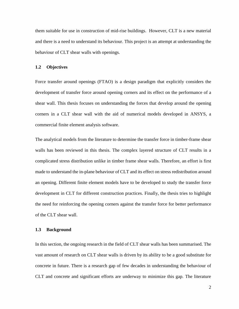
1.4 Overview of the Thesis
Finite element modeling is the primary approach adopted in this thesis to study the
development of transfer force in CLT shear walls with openings. A library of finite element
models has been developed in this thesis to analyse CLT shear walls with openings constructed
using different practices, which is shown in Figure 1.1.
Figure 1.1 Overview of finite element models

9
Figure 1.1 presents four finite element models that have been developed in this thesis using
ANSYS. Model A is a continuum model developed using quadrilateral 4-node elements for
studying the analytical models discussed in Chapter 2. Model B is a 3-dimensional model
developed using 8-noded brick elements. Model C is a frame model that has been developed
using 2-noded beam elements. The development of Model B and Model C is discussed in
Chapter 3 for analysing a CLT shear walls with a cut-out opening. Model D is a continuum
model calibrated to experimental data, which has been is discussed in Chapter 4 for analysing
coupled-panel CLT shear walls.
The thesis is structured to adopt a step-by-step approach for understanding the transfer force
development in CLT and corresponding reinforcement requirements. The second chapter
reviews the various analytical models available in the literature to determine the transfer force.
A finite element model is also presented, i.e., Model A, which can provide the transfer force.
The finite element model clearly shows the stress concentration at corners of the opening,
leading to the development of transfer force.
In the third chapter, the in-plane behaviour of CLT has been first explained. CLT shear walls
with cut-out openings have been analysed in this chapter using Model B and Model C. The
results from the analysis suggest that stress concentration around opening corners can lead to
shear failure in the wood panels for large openings.
The fourth chapter focuses on development of a finite element model, i.e., Model D, to study
the behaviour of coupled panel CLT shear walls with opening. Tie-rods have been used in this
case as reinforcement around the opening corners. The analysis results suggest that the use of
tie-rods significantly increases the strength and stiffness of the wall.

10
In the fifth chapter, the development of a regression model for in-plane stiffness of a simply-
supported CLT shear wall with a window-type opening is explained. The regression analysis
indicates the effect of various geometrical and material parameters on the stiffness of the wall.
The sixth chapter provides the conclusion of the thesis with emphasis on highlighting the
manner in which this thesis addresses the present research gap. The chapter also provides
directions of research that can be explored in future for design of CLT shear walls for the
transfer force around opening corners.
11
Chapter 2: Analytical Models for Force Transfer around Openings
Force transfer around openings (FTAO) is an approach suggested in the International building
code for design of shear walls with openings. The objective of this approach is to ensure that
the wall deforms as a single unit. In the presence of an opening, stress concentration occurs
around the corners of the opening. These stress concentrations lead to development of tensile
and compressive forces at the corners of the opening, which leads to deformation of wall at the
opening corners. In FTAO design approach, reinforcements are provided at the corners to carry
these forces to minimize the deformations around the opening corners. The tensile and
compressive forces developing at the corners are called as transfer forces. In the literature,
various analytical models are available to compute this transfer force. In this chapter, few of
these models have been explained. Furthermore, the application of these models on an example
shear wall is demonstrated. Based on this example and from literature, the advantages and
disadvantages of using these models and their applicability to CLT shear walls is studied.
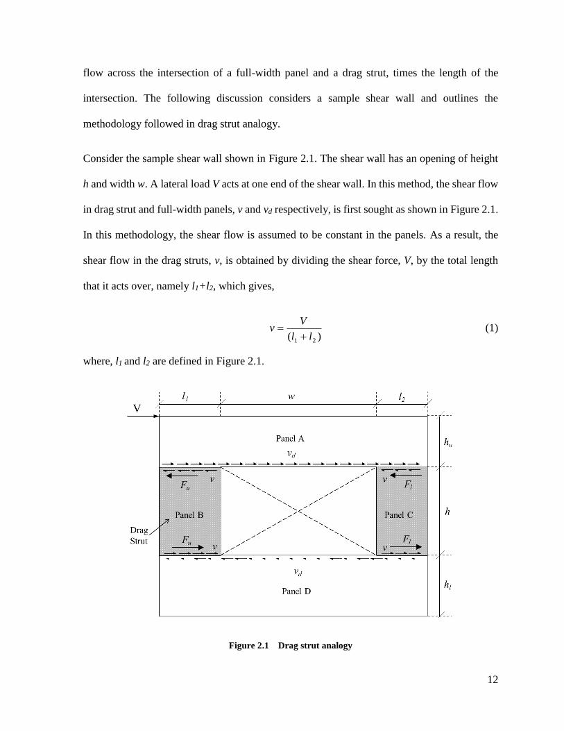
2.1 Drag Strut Analogy
Drag strut analogy is the simplest method to determine FTAO (Martin 2005). A drag strut is a
structural member that distributes the forces within a shear wall. In this analogy, it is
considered that the panels on either side of the opening act as drag struts transferring the load
from the full-width Panel A to full-width Panel D as shown in Figure 2.1. Panel B and Panel
C are grey shaded in Figure 2.1 to highlight their function as drag struts. The analogy considers
that the shear flow is constant in the horizontal direction and varies only at the boundary of the
full-width panels with the drag struts. The transfer force develops due to the change in shear
flow from one panel to another. Hence, the transfer force is computed as the difference in shear
12
flow across the intersection of a full-width panel and a drag strut, times the length of the
intersection. The following discussion considers a sample shear wall and outlines the
methodology followed in drag strut analogy.
Consider the sample shear wall shown in Figure 2.1. The shear wall has an opening of height
h and width w. A lateral load V acts at one end of the shear wall. In this method, the shear flow
in drag strut and full-width panels, v and vd respectively, is first sought as shown in Figure 2.1.
In this methodology, the shear flow is assumed to be constant in the panels. As a result, the
shear flow in the drag struts, v, is obtained by dividing the shear force, V, by the total length
that it acts over, namely l1+l2, which gives,
)( 21 ll
Vv
(1)
where, l1 and l2 are defined in Figure 2.1.
Figure 2.1 Drag strut analogy
13
Similarly, vd is obtained by dividing the shear force, V, by the total length that it acts over i.e.,
l1+w+l2, which gives
)( 21 lwl
Vvd
(2)
where, l1, l2 and w are defined in Figure 2.1.
Next, consider the intersection between Panel A and Panel B. The length of intersection
between the panels is l1. The shear flow in Panel A is v and shear flow in Panel B is vd. The
force developed in Panel A at the intersection is the shear flow, v, times the intersection length,
l1. Similarly, the force developed in Panel B at the intersection is the shear flow, vd, times the
intersection length, l1. This shows that at the intersection, the forces are not balanced. This
difference in force is the transfer force. Hence, the transfer force, Fu, developed at the
intersection of Panel A and Panel B is given as,
)(1 du vvlF (3)
The drag strut, Panel B, is under equilibrium. Hence, by balancing the forces on this panel, the
transfer force developing at the intersection of Panel B and Panel D can be shown to be equal
and opposite to Fu, as shown in Figure 2.1.
On the other side of the opening, transfer force, Fl, develops at the intersection between Panel
A and Panel C. The panels overlap with an intersection length l2. The shear flow in panel A
and Panel C is vd and v, respectively. The force developed in Panel A at the intersection is the
shear flow, v, times the intersection length, l2. Similarly, the force developed in Panel C at the
intersection is the shear flow, vd, times the intersection length, l2. As done previously, the

14
transfer force Fl is computed as the difference in force across the intersection. The transfer
force, Fl, developed at the intersection of Panel A and Panel B is given as,
)(2 vvlF dl (4)
The drag strut, Panel C, is under equilibrium. Hence, by balancing the forces on this panel, the
transfer force developing at the intersection of Panel C and Panel D can be shown to be equal
and opposite to Fl, as shown in Figure 2.1.
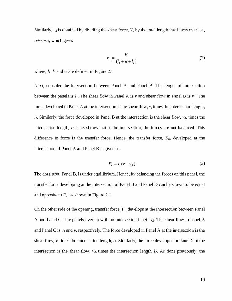
2.2 Cantilever Beam Analogy
Cantilevered beam analogy is another model for determining FTAO (Martin 2005). For the
purpose of analysis based on this model, the wall is divided into panels as shown in Figure 2.2.
The transfer force is computed in this model as the reaction force exerted by the full-height
panels on either side of the opening on the panels above and below the opening. The
computation of this reaction force is complex and the model considers few assumptions to
simplify the problem to attain an analytical solution. Firstly, the model assumes an inflection
point at the mid-height of the opening. A horizontal section X-X through this point divides the
full-height piers on both sides of the opening into Panel A, Panel B, Panel C and Panel D as
shown in Figure 2.2. Along this section the bending moment is zero as the shear force does not
vary along the height. Hence, these panels act as cantilevered piers with Panel E and Panel F
as supports. In the presence of the opening, the shear flow is assumed to be distributed equally
to panels above and below the opening. The shear flow from the cantilevered piers to the
supports leads to the development of reaction forces in supports. These reaction forces act as
a moment-couple as shown in Figure 2.2. The resolution of this moment couple helps to
15
determine the reaction force. The following section considers a single panel and analyses it to
highlight the steps involved in the methodology.
Figure 2.2 Cantilevered beam analogy
Firstly, consider the full-height panel to the left of the opening. As shown in Figure 2.3 (a),
this panel is divided into two cantilevered piers, i.e., Panel A and Panel B by the horizontal
section X-X. A lateral load V is applied on the shear wall, which leads to the development of
a shear force V in the shear wall. The corresponding shear flow that develops varies in
horizontal and vertical directions in each pier. But, in this model, the shear flow in each pier is
assumed to be constant. At section X-X, the net shear force is V, which acts over a length l1+l2.
Hence, the shear flow, v, in the cantilevered piers is given as,
)( 21 ll
Vv (5)
16
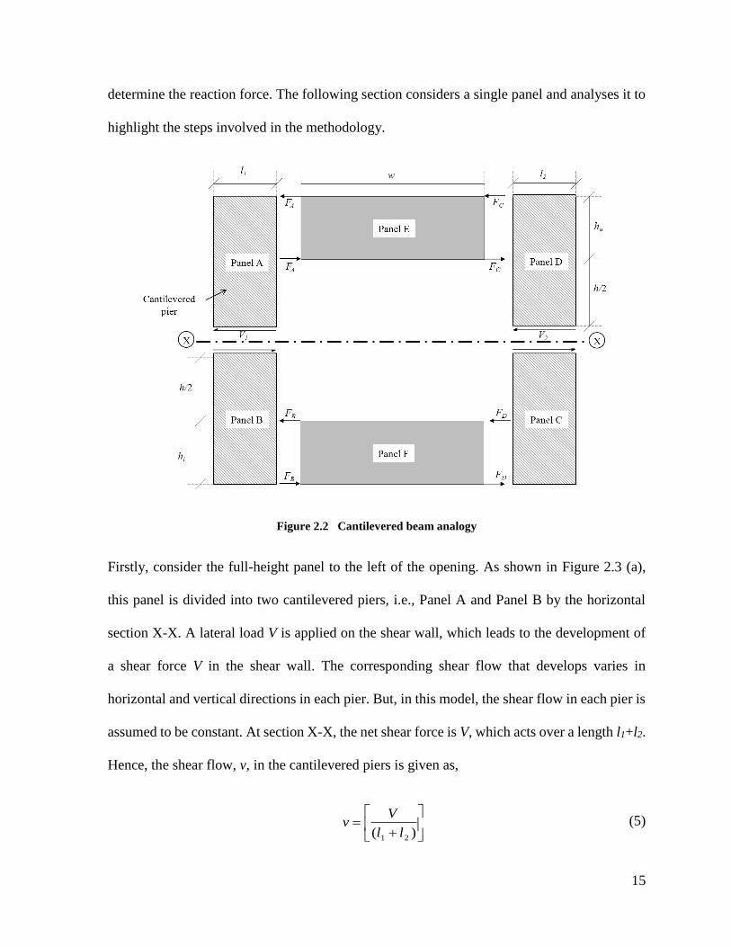
where, l1 and l2 are the width of the full-height panels on either side of the opening as shown
in Figure 2.2. Therefore, the shear force, V1, developed in Panel A and Panel B, of width l1, is
given as,
)( 21
11
ll
lVV (6)
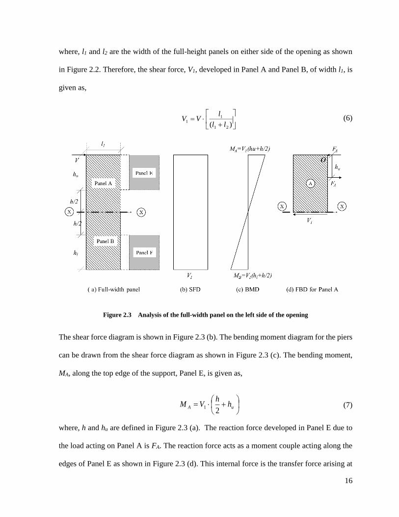
Figure 2.3 Analysis of the full-width panel on the left side of the opening
The shear force diagram is shown in Figure 2.3 (b). The bending moment diagram for the piers
can be drawn from the shear force diagram as shown in Figure 2.3 (c). The bending moment,
MA, along the top edge of the support, Panel E, is given as,
uA h
hVM
21 (7)
where, h and hu are defined in Figure 2.3 (a). The reaction force developed in Panel E due to
the load acting on Panel A is FA. The reaction force acts as a moment couple acting along the
edges of Panel E as shown in Figure 2.3 (d). This internal force is the transfer force arising at
17
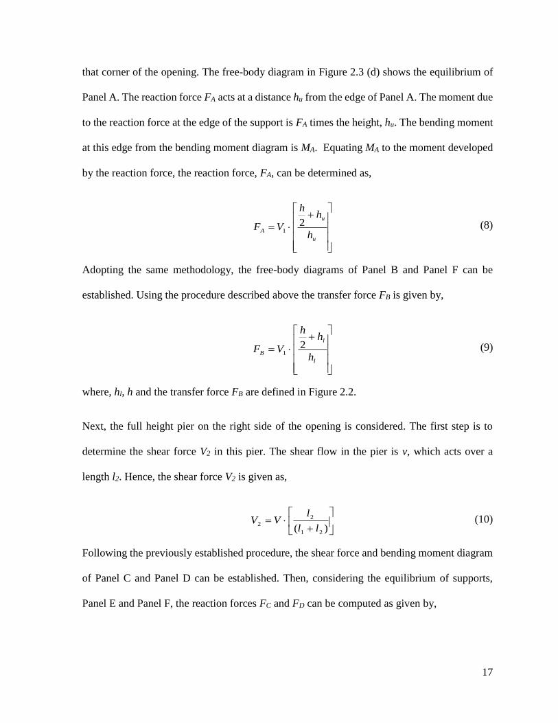
that corner of the opening. The free-body diagram in Figure 2.3 (d) shows the equilibrium of
Panel A. The reaction force FA acts at a distance hu from the edge of Panel A. The moment due
to the reaction force at the edge of the support is FA times the height, hu. The bending moment
at this edge from the bending moment diagram is MA. Equating MA to the moment developed
by the reaction force, the reaction force, FA, can be determined as,
u
u
Ah
hh
VF 21
(8)
Adopting the same methodology, the free-body diagrams of Panel B and Panel F can be
established. Using the procedure described above the transfer force FB is given by,
l
l
Bh
hh
VF 21
(9)
where, hl, h and the transfer force FB are defined in Figure 2.2.
Next, the full height pier on the right side of the opening is considered. The first step is to
determine the shear force V2 in this pier. The shear flow in the pier is v, which acts over a
length l2. Hence, the shear force V2 is given as,
)( 21
2
2ll
lVV (10)
Following the previously established procedure, the shear force and bending moment diagram
of Panel C and Panel D can be established. Then, considering the equilibrium of supports,
Panel E and Panel F, the reaction forces FC and FD can be computed as given by,
18
u
u
Ch
hh
VF 22
(11)
l
l
Dh
hh
VF 22
(12)
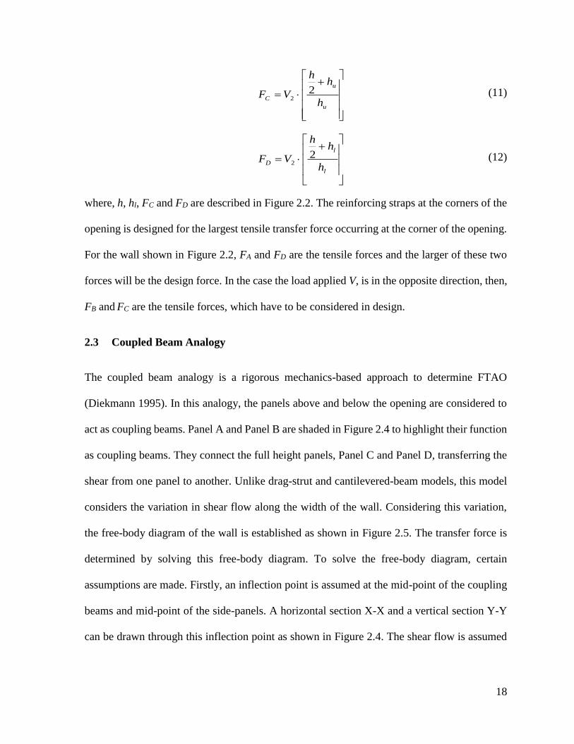
where, h, hl, FC and FD are described in Figure 2.2. The reinforcing straps at the corners of the
opening is designed for the largest tensile transfer force occurring at the corner of the opening.
For the wall shown in Figure 2.2, FA and FD are the tensile forces and the larger of these two
forces will be the design force. In the case the load applied V, is in the opposite direction, then,
FB and FC are the tensile forces, which have to be considered in design.
2.3 Coupled Beam Analogy
The coupled beam analogy is a rigorous mechanics-based approach to determine FTAO
(Diekmann 1995). In this analogy, the panels above and below the opening are considered to
act as coupling beams. Panel A and Panel B are shaded in Figure 2.4 to highlight their function
as coupling beams. They connect the full height panels, Panel C and Panel D, transferring the
shear from one panel to another. Unlike drag-strut and cantilevered-beam models, this model
considers the variation in shear flow along the width of the wall. Considering this variation,
the free-body diagram of the wall is established as shown in Figure 2.5. The transfer force is
determined by solving this free-body diagram. To solve the free-body diagram, certain
assumptions are made. Firstly, an inflection point is assumed at the mid-point of the coupling
beams and mid-point of the side-panels. A horizontal section X-X and a vertical section Y-Y
can be drawn through this inflection point as shown in Figure 2.4. The shear flow is assumed
19
to be constant along these sections. Below, the analysis procedure is explained to determine
the transfer force based on the coupled-beam model.
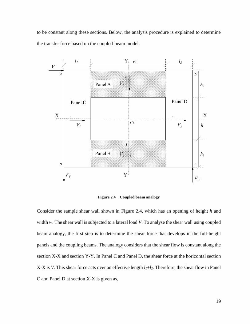
Figure 2.4 Coupled beam analogy
Consider the sample shear wall shown in Figure 2.4, which has an opening of height h and
width w. The shear wall is subjected to a lateral load V. To analyse the shear wall using coupled
beam analogy, the first step is to determine the shear force that develops in the full-height
panels and the coupling beams. The analogy considers that the shear flow is constant along the
section X-X and section Y-Y. In Panel C and Panel D, the shear force at the horizontal section
X-X is V. This shear force acts over an effective length l1+l2. Therefore, the shear flow in Panel
C and Panel D at section X-X is given as,
20
)( 21 ll
Vv (13)
where, l1 and l2 are defined in Figure 2.4. In Panel C, the shear flow v acts over a length l1 to
develop a shear force V1, which is given as,
)( 21
11
ll
lVV (14)
Similarly, in Panel D, the shear flow v acts over a length l2 to develop a shear force V2, which
is given as,
)( 21
22
ll
lVV (15)
Next, the shear force in the coupling beams, Panel A and Panel B has to be determined. Prior
to determining the shear force in the coupling beams, it is useful to determine the reaction force
that develops at the base of the shear wall to prevent overturning. The hold-downs for the shear
wall are provided at B and C. The reaction forces at these hold-downs are FT and FC,
respectively, as shown in Figure 2.4. The reaction force FT can be calculated by considering
the equilibrium of the shear wall about C. The lateral load V acts at distance hu+h+hl from point
C. The clockwise moment due to the lateral load is V times the distance hu+h+hl. The reaction
force in the hold-down, FT, acts at a distance l1+w+l2 from the point C. The counter-clockwise
moment produced by this force is calculated as the reaction force FT multiplied by the distance
from point C, i.e., l1+w+l2. As the net moment at point C is zero, equating the moments, FT,
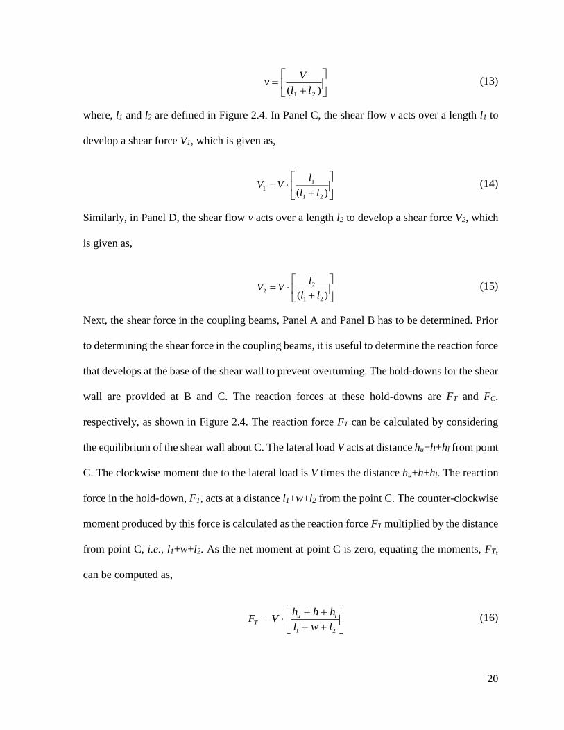
can be computed as,
21 lwl
hhhVF lu
T (16)
21
where, hu, h, hl, l1, w and l2 are defined in Figure 2.4. The net force in the vertical direction is
zero. This implies that the reaction force at the other hold-down, FC, is equal and opposite of
FT.
After obtaining the reaction forces, the shear forces in the coupling beams can also be
calculated. The horizontal section X-X and vertical section Y-Y divide the shear wall into four
quadrants. Consider the top left quadrant of Figure 2.4, which consists of a segment of Panel
C and Panel A. The quantity of interest here is the shear force, V3, which develops in the
coupling beam, Panel A. The shear force, V3, in this beam is constant along its length w. To
compute this shear force, the equilibrium of the quadrant is considered. The quadrant is under
stable equilibrium. Therefore, the net moment of all forces acting on this quadrant, i.e., V1 and
V3, about any point on the quadrant is zero. Consider the net moment about point A due to the
forces V1 and V3. V1 is the shear force in Panel C, which acts at a distance l1+w/2 from the point
A. V3, acts at a distance hu+h/2 from the point A. Equating the net moment at A due to V1 and
V3 to zero , V3 is given as,
2
2
1
13 wl
hh
VVu
(17)
Next, the shear force, V4, in the other coupling beam, Panel B is determined. To compute this
shear force, consider the sum of vertical forces at the section Y-Y shown in Figure 2.4. The
net force at the section is the reaction force FT. This implies that the sum of V3 and V4 should
be equal to FT. Hence, V4 is given as
34 VFV T (18)
22
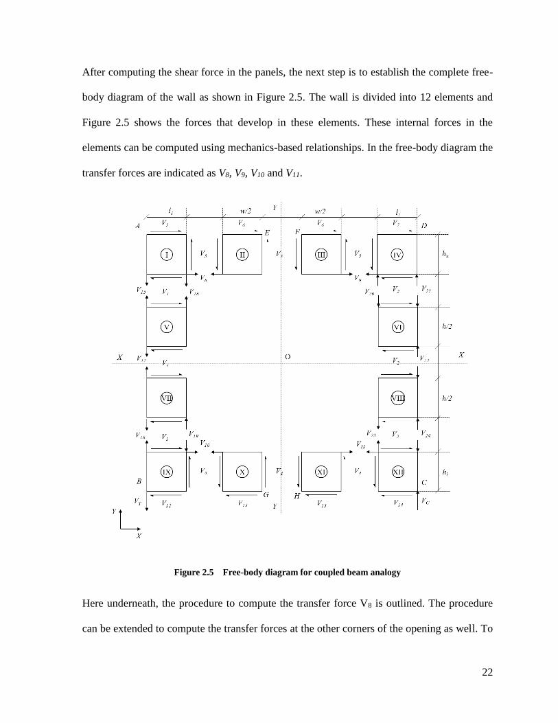
After computing the shear force in the panels, the next step is to establish the complete free-
body diagram of the wall as shown in Figure 2.5. The wall is divided into 12 elements and
Figure 2.5 shows the forces that develop in these elements. These internal forces in the
elements can be computed using mechanics-based relationships. In the free-body diagram the
transfer forces are indicated as V8, V9, V10 and V11.
Figure 2.5 Free-body diagram for coupled beam analogy
Here underneath, the procedure to compute the transfer force V8 is outlined. The procedure
can be extended to compute the transfer forces at the other corners of the opening as well. To
23
compute V8, consider the element II shown in Figure 2.5. This element is under equilibrium.
Therefore, the sum of moments created by all internal forces on this element about any point
on it is zero. So, consider the moment of all internal forces in the element about a point E, as
shown in Figure 2.5. The force V3 acts at a distance w/2 from the point E and creates a counter-
clockwise moment. The transfer force V8 acts at a distance hu from the point E, creating a
clockwise moment. As the sum of moments about point E is zero, V8 is given as,
uh
wV
V 23
8 (19)
where, w and hu are defined in Figure 2.5. Similarly, the transfer force V9, V10 and V11 can be
obtained. To determine the transfer force V9, consider moment about point F for element III.
Considering the equilibrium of element III about point F, the transfer force V9 is given as,
uh
wV
V 23
9 (20)
The transfer force V10 can be determined by considering moment about point G for element X.
Considering the equilibrium of element X about point G, the transfer force V10 is given as,
lh
wV
V 24
10 (21)
Similarly, the transfer force V11 is computed by considering the equilibrium of element XI
about point H. The transfer force V10 is given as,
24
lh
wV
V 24
11 (22)
A limitation of this method is that the minimum panel height above opening has to be 12 inches
(Yeh et al. 2011). A lower height results in large resolved shear forces causing overstressing
of the panel.
2.4 Diekmann Method
The Diekmann method is a variation of the coupled-beam analogy described in section 2.3.
The method was suggested by Edward Diekmann in response to the comparison of methods
presented by Martin (Martin 2005). The lateral load applied on the wall produces a horizontal
shear, which is resisted by the panels on either side of the opening. This is considered for
analysis in the drag-strut analogy and cantilevered beam analogy. But, the hold-down forces
produces a vertical shear in the panels above and below the opening. This effect is not
considered in drag-strut analogy and cantilevered beam analogy. By considering this effect,
the free-body diagram for the wall can be established, which is similar to the one shown in
Figure 2.5. The difference between coupled beam analogy and the Diekmann method is the
approach used to determine the vertical shear developing in the wall. Below, a simplified
methodology is explained to determine the transfer force based on the Diekmann model.
Consider the shear wall shown in Figure 2.6. The shear wall has an opening of height h and a
width w. The wall is analysed for a lateral load V applied along the top edge. The wall is
connected to the floor at its two bottom corners by hold-downs. The hold-downs develop
resisting force, which can be determined by equating the overturning moment from the lateral
load V to the resisting moment developed by the hold-down forces. The tensile hold-down
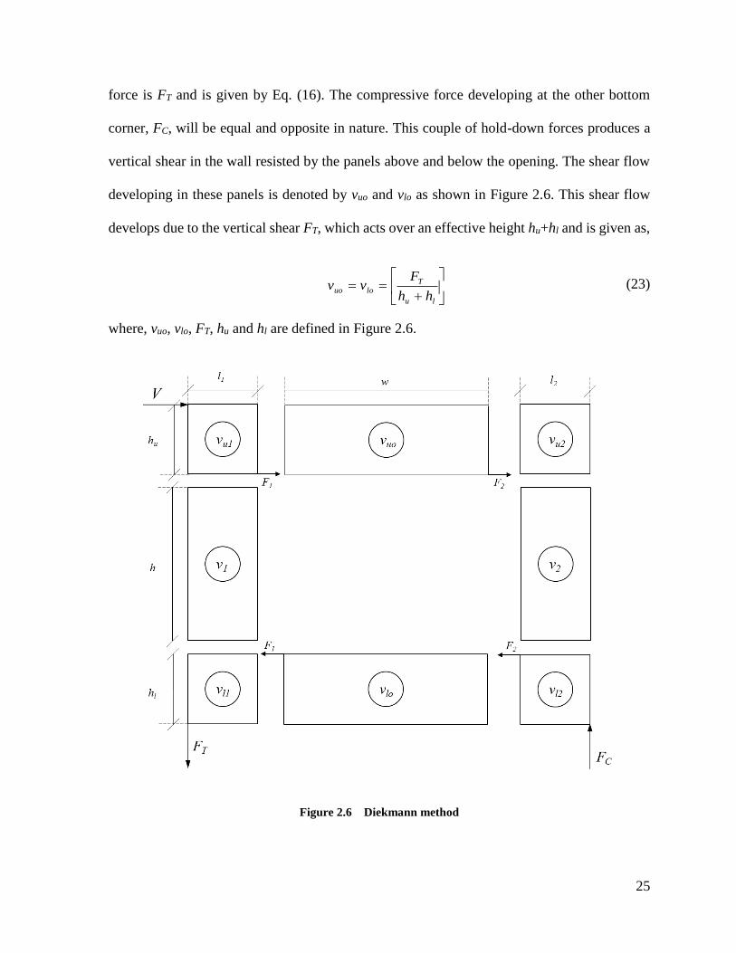
25
force is FT and is given by Eq. (16). The compressive force developing at the other bottom
corner, FC, will be equal and opposite in nature. This couple of hold-down forces produces a
vertical shear in the wall resisted by the panels above and below the opening. The shear flow
developing in these panels is denoted by vuo and vlo as shown in Figure 2.6. This shear flow
develops due to the vertical shear FT, which acts over an effective height hu+hl and is given as,
lu
Tlouo
hh
Fvv (23)
where, vuo, vlo, FT, hu and hl are defined in Figure 2.6.
Figure 2.6 Diekmann method
26
The shear flow in the panels above and below the opening are assumed to create a boundary
force at the top and bottom edge of the opening. This boundary force, FB, is the product of
shear flow in the panel, vuo or vlo, and the length that it acts over, i.e., w, which is given as,
wvF uoB (24)
where, w is the width of the opening over which the unit shear, vuo, acts. The boundary force,
FB, is distributed to the corners of the opening based on the relative width of the panels on
either side of the opening. This distributed force at the corner is the transfer force. Therefore,
the transfer force in the left-hand side top corner of the opening, F1, is given as,
21
1
1ll
lFF B
(25)
where, l1 and l2 are defined in Figure 2.6. Similarly, the transfer force at the right hand top
corner of the opening, F2, is given as,
21
22
ll
lFF B
(26)
The model as previously mentioned, works by developing the free-body diagram. Hence, the
other forces in the boundary members can be computed. These forces in boundary members,
though not the transfer force, are important in design of the structural members composing the
wall.
The above sections explain the analytical models available to determine the design transfer
force. In the next section, an example shear-wall will be analyzed. The results will be compared
with those from a finite element model in order to assess the accuracy of the previously
presented analytical methods.
27
2.5 Numerical Example
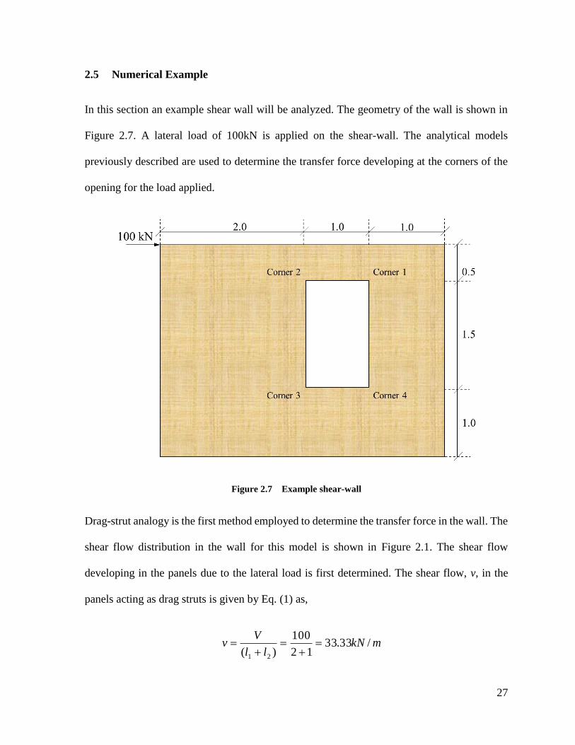
In this section an example shear wall will be analyzed. The geometry of the wall is shown in
Figure 2.7. A lateral load of 100kN is applied on the shear-wall. The analytical models
previously described are used to determine the transfer force developing at the corners of the
opening for the load applied.
Figure 2.7 Example shear-wall
Drag-strut analogy is the first method employed to determine the transfer force in the wall. The
shear flow distribution in the wall for this model is shown in Figure 2.1. The shear flow
developing in the panels due to the lateral load is first determined. The shear flow, v, in the
panels acting as drag struts is given by Eq. (1) as,
mkNll
Vv /33.33
12
100
)( 21
28
Similarly, the shear flow, vd, in the full-width panels above and below the opening is given by
Eq. (2) as,
mkNlwl
Vvd /00.25
112
100
)( 21
The difference in shear flow is assumed to produce the transfer force at the corners of the
opening. The transfer force, Fu, at the left-hand top corner of the opening is given by Eq. (3)
as,
kNvvlF du 67.1600.2533.3321
Similarly, the transfer force, Fl, at the right-hand top corner of the opening is given by Eq. (4)
as,
kNvvlF dl 33.833.3300.2512
The next model used to compute the transfer force is the cantilevered beam analogy. The
division of the wall into panels for analysis using this model is shown in Figure 2.2. The first
step is to compute the shear flow in each panel due to the lateral load. The shear flow, v, in the
cantilever piers on either side of the opening is given by Eq. (5) as,
mkNll
Vv /33.33
12
100
)( 21
29
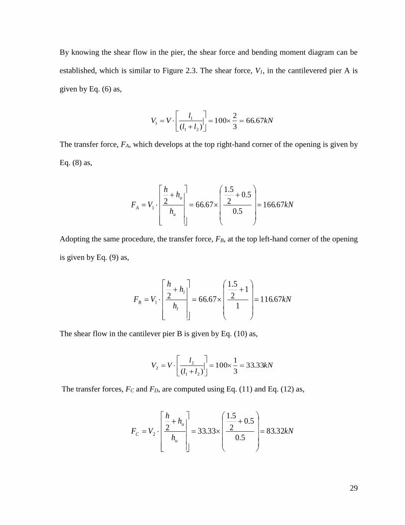
By knowing the shear flow in the pier, the shear force and bending moment diagram can be
established, which is similar to Figure 2.3. The shear force, V1, in the cantilevered pier A is
given by Eq. (6) as,
kNll
lVV 67.66
3
2100
)( 21
1
1
The transfer force, FA, which develops at the top right-hand corner of the opening is given by
Eq. (8) as,
kNh
hh
VFu
u
A 67.1665.0
5.02
5.1
67.6621
Adopting the same procedure, the transfer force, FB, at the top left-hand corner of the opening
is given by Eq. (9) as,
kNh
hh
VFl
l
B 67.1161
12
5.1
67.6621
The shear flow in the cantilever pier B is given by Eq. (10) as,
kNll
lVV 33.33
3
1100
)( 21
2
2
The transfer forces, FC and FD, are computed using Eq. (11) and Eq. (12) as,
kNh
hh
VFu
u
C 32.835.0
5.02
5.1
33.3322
30
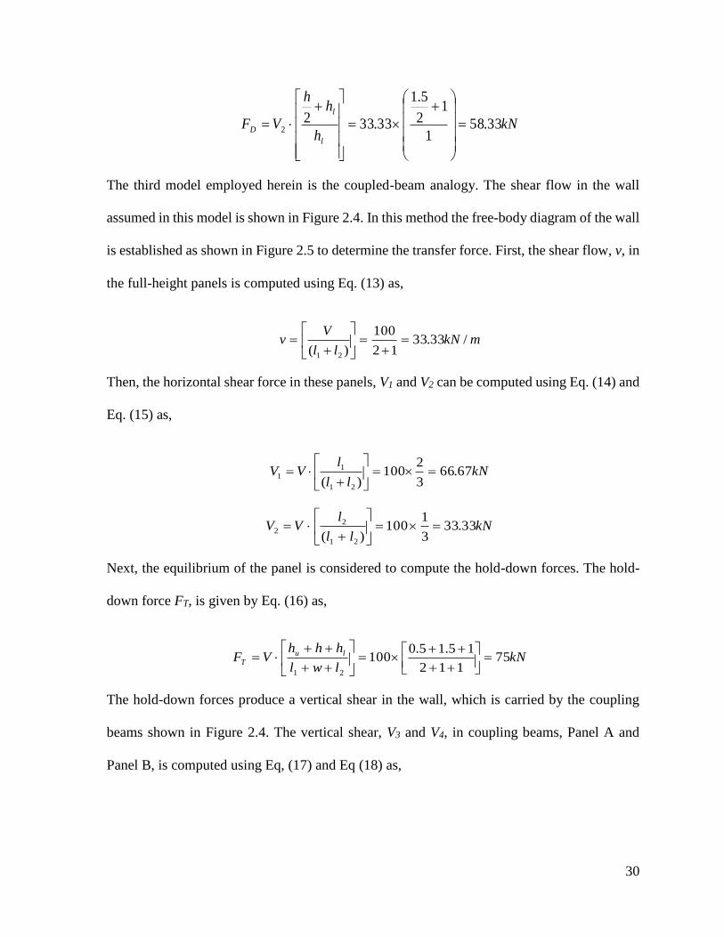
kNh
hh
VFl
l
D 33.581
12
5.1
33.3322
The third model employed herein is the coupled-beam analogy. The shear flow in the wall
assumed in this model is shown in Figure 2.4. In this method the free-body diagram of the wall
is established as shown in Figure 2.5 to determine the transfer force. First, the shear flow, v, in
the full-height panels is computed using Eq. (13) as,
mkNll
Vv /33.33
12
100
)( 21
Then, the horizontal shear force in these panels, V1 and V2 can be computed using Eq. (14) and
Eq. (15) as,
kNll
lVV 67.66
3
2100
)( 21
1
1
kNll
lVV 33.33
3
1100
)( 21
22
Next, the equilibrium of the panel is considered to compute the hold-down forces. The hold-
down force FT, is given by Eq. (16) as,
kNlwl
hhhVF lu
T 75112
15.15.0100
21
The hold-down forces produce a vertical shear in the wall, which is carried by the coupling
beams shown in Figure 2.4. The vertical shear, V3 and V4, in coupling beams, Panel A and
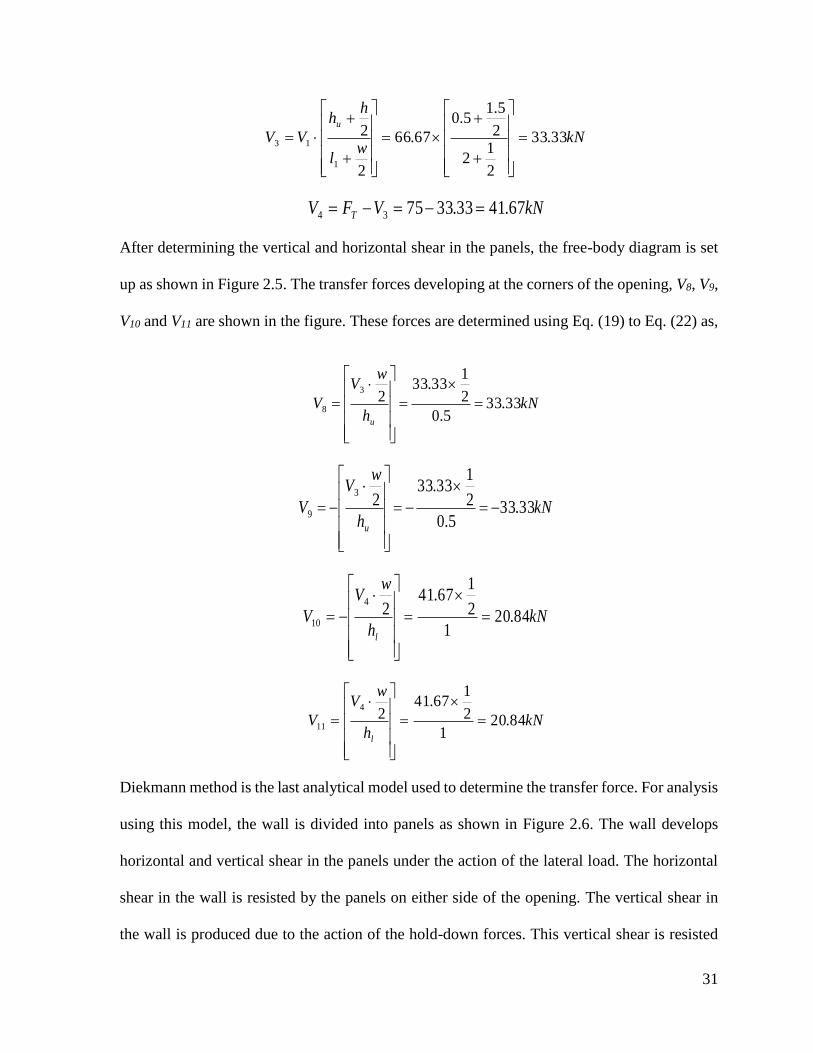
Panel B, is computed using Eq, (17) and Eq (18) as,
31
kNw
l
hh
VVu
33.33
2
12
2
5.15.0
67.66
2
2
1
13
kNVFV T 67.4133.337534
After determining the vertical and horizontal shear in the panels, the free-body diagram is set
up as shown in Figure 2.5. The transfer forces developing at the corners of the opening, V8, V9,
V10 and V11 are shown in the figure. These forces are determined using Eq. (19) to Eq. (22) as,
kNh
wV
Vu
33.335.0
2
133.33
23
8
kNh
wV
Vu
33.335.0
2
133.33
23
9
kNh
wV
Vl
84.201
2
167.41
24
10
kNh
wV
Vl
84.201
2
167.41
24
11
Diekmann method is the last analytical model used to determine the transfer force. For analysis
using this model, the wall is divided into panels as shown in Figure 2.6. The wall develops
horizontal and vertical shear in the panels under the action of the lateral load. The horizontal
shear in the wall is resisted by the panels on either side of the opening. The vertical shear in
the wall is produced due to the action of the hold-down forces. This vertical shear is resisted
32
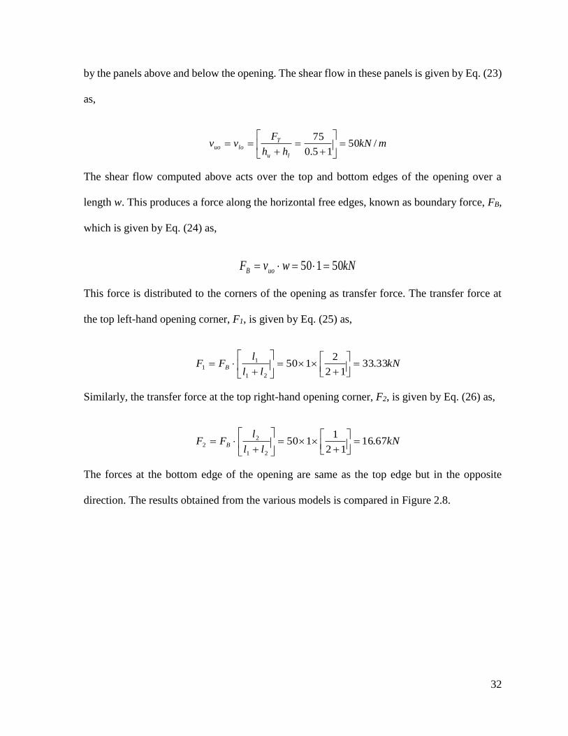
by the panels above and below the opening. The shear flow in these panels is given by Eq. (23)
as,
mkNhh
Fvv
lu
Tlouo /50
15.0
75
The shear flow computed above acts over the top and bottom edges of the opening over a
length w. This produces a force along the horizontal free edges, known as boundary force, FB,
which is given by Eq. (24) as,
kNwvF uoB 50150
This force is distributed to the corners of the opening as transfer force. The transfer force at
the top left-hand opening corner, F1, is given by Eq. (25) as,
kNll
lFF B 33.33
12
2150
21
11
Similarly, the transfer force at the top right-hand opening corner, F2, is given by Eq. (26) as,
kNll
lFF B 67.16
12
1150
21
22
The forces at the bottom edge of the opening are same as the top edge but in the opposite
direction. The results obtained from the various models is compared in Figure 2.8.
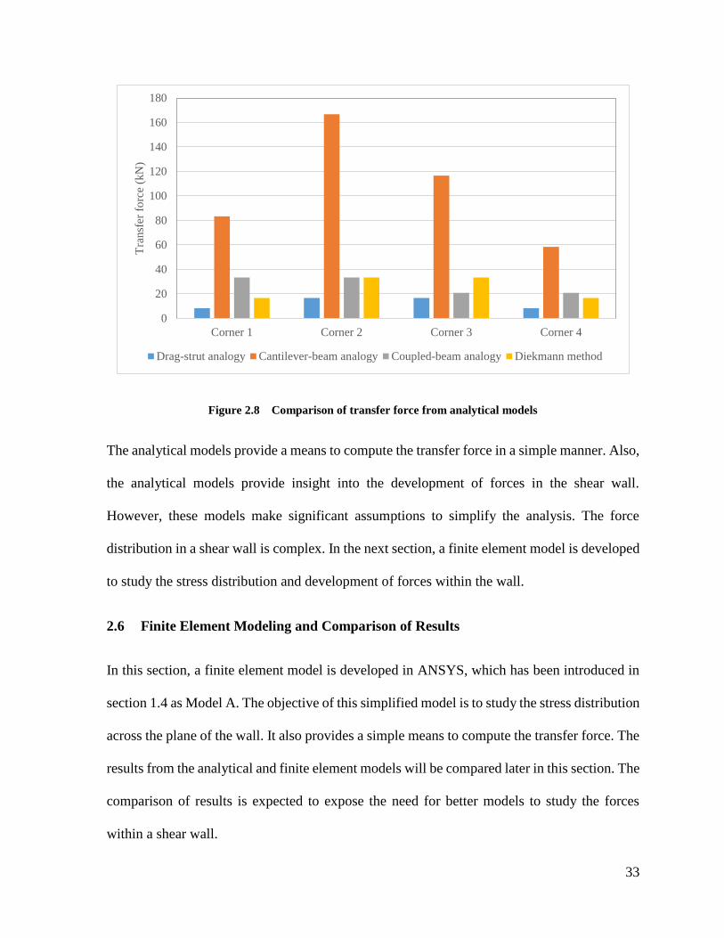
33
Figure 2.8 Comparison of transfer force from analytical models
The analytical models provide a means to compute the transfer force in a simple manner. Also,
the analytical models provide insight into the development of forces in the shear wall.
However, these models make significant assumptions to simplify the analysis. The force
distribution in a shear wall is complex. In the next section, a finite element model is developed
to study the stress distribution and development of forces within the wall.
2.6 Finite Element Modeling and Comparison of Results
In this section, a finite element model is developed in ANSYS, which has been introduced in
section 1.4 as Model A. The objective of this simplified model is to study the stress distribution
across the plane of the wall. It also provides a simple means to compute the transfer force. The
results from the analytical and finite element models will be compared later in this section. The
comparison of results is expected to expose the need for better models to study the forces
within a shear wall.
0
20
40
60
80
100
120
140
160
180
Corner 1 Corner 2 Corner 3 Corner 4
Tra
nsf
er f
orc
e (k
N)
Drag-strut analogy Cantilever-beam analogy Coupled-beam analogy Diekmann method
34
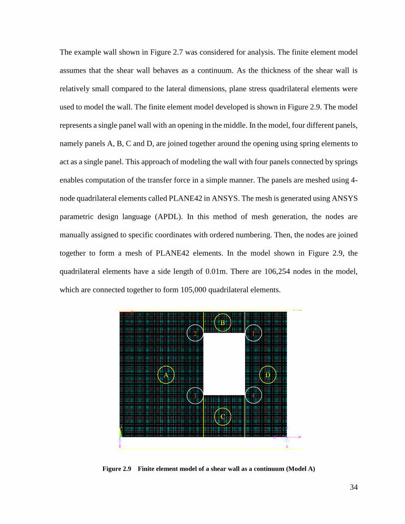
The example wall shown in Figure 2.7 was considered for analysis. The finite element model
assumes that the shear wall behaves as a continuum. As the thickness of the shear wall is
relatively small compared to the lateral dimensions, plane stress quadrilateral elements were
used to model the wall. The finite element model developed is shown in Figure 2.9. The model
represents a single panel wall with an opening in the middle. In the model, four different panels,
namely panels A, B, C and D, are joined together around the opening using spring elements to
act as a single panel. This approach of modeling the wall with four panels connected by springs
enables computation of the transfer force in a simple manner. The panels are meshed using 4-
node quadrilateral elements called PLANE42 in ANSYS. The mesh is generated using ANSYS
parametric design language (APDL). In this method of mesh generation, the nodes are
manually assigned to specific coordinates with ordered numbering. Then, the nodes are joined
together to form a mesh of PLANE42 elements. In the model shown in Figure 2.9, the
quadrilateral elements have a side length of 0.01m. There are 106,254 nodes in the model,
which are connected together to form 105,000 quadrilateral elements.
Figure 2.9 Finite element model of a shear wall as a continuum (Model A)
35
The four panels in the model are joined together using spring elements. In Figure 2.9, the
vertical lines (shown in yellow) emanating from the corners of the opening show the
intersection of the panels. The springs connecting the panels are distributed along these lines.
At the intersection, every node from either adjoining panel is connected using a pair of springs.
One spring acts in the horizontal direction and the other acts in the vertical direction, carrying
the forces that develop between the panels. Both the springs are unidirectional zero length
springs with high stiffness in the direction of orientation. The quadrilateral elements used to
mesh the panels have two degrees of freedom, translation in X and Y direction denoted as UX
and UY. This paired set of springs connect the degrees of freedom of the quadrilateral elements
across the intersection. The next aspect considered in modeling is the loading and boundary
conditions. The shear wall is considered to be simply-supported at the base as shown in Figure
2.9. A lateral load of 100kN is applied at the top left-hand corner of the wall.
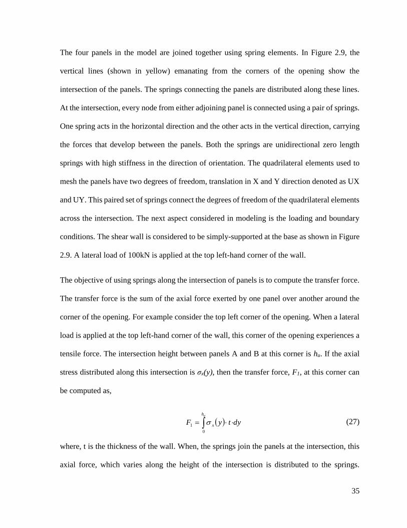
The objective of using springs along the intersection of panels is to compute the transfer force.
The transfer force is the sum of the axial force exerted by one panel over another around the
corner of the opening. For example consider the top left corner of the opening. When a lateral
load is applied at the top left-hand corner of the wall, this corner of the opening experiences a
tensile force. The intersection height between panels A and B at this corner is hu. If the axial
stress distributed along this intersection is σx(y), then the transfer force, F1, at this corner can
be computed as,
dytyFuh
x 0
1 (27)
where, t is the thickness of the wall. When, the springs join the panels at the intersection, this
axial force, which varies along the height of the intersection is distributed to the springs.

36
Therefore, the transfer force can be computed by summing the force in the springs at the
corners of the opening. For instance, the transfer force at the top left-hand corner of the opening
is computed by summing the tensile forces in the springs at the intersection between panels A
and B. Similarly, using the model, the transfer force at the other corners of the opening can be
computed. The transfer force computed at the corners of the opening is summarized in Table
2.1. The notation of corner numbers is shown in Figure 2.9.
Corner 1 Corner 2 Corner 3 Corner 4
-18.46 kN 30.32 kN -27.39 kN 12.10 kN
Table 2.1 Transfer force from the finite element model
Figure 2.10 Deformed shape of the wall under the action of a lateral load

37
The design transfer force is the maximum tensile transfer force that can develop at the corners
of the opening. The design transfer force is used to design reinforcing straps at the corners of
the opening. These reinforcing straps carry the tensile force preventing damage at the corners
of the opening. Figure 2.11 compares the transfer force obtained from the different analytical
models and the finite element model.
Figure 2.11 Comparison of design transfer force obtained from different models
The comparison in Figure 2.11 clearly shows the variation in results from different models.
The transfer force obtained from the finite element model can be considered as the most
reliable due to the better approximation of stress distribution in this model. Compared to the
finite element model, the drag-strut analogy severely under predicts the design transfer force
and the cantilever-beam model severely over predicts the design transfer force. This variation
in results obtained from these two models is mainly due to the assumptions made in the shear
flow distribution. The coupled-beam analogy and the Diekmann model provide reasonably
0
20
40
60
80
100
120
140
160
180
Corner 1 Corner 2 Corner 3 Corner 4
Tra
nsf
er f
orc
e (k
N)
Drag-strut analogy Cantilever-beam analogy Coupled-beam analogy
Diekmann method FE model
38
good approximation of the transfer force when compared to the finite element model. This
improvement in the result is primarily due to more detailed consideration of the shear flow
variation at different sections of the wall. The trend observed here is well documented in the
literature as well (Li et al. 2012; Robertson 2009). The Diekmann model has been regarded as
the most suitable model for determining the transfer force for window-type openings. The
coupled-beam analogy and the Diekmann method are based on establishing the free-body
diagram. The computation of shear flow in the panels is a pre-requisite for developing the free-
body diagram. In the presence of a door-type opening, the coupled-beam analogy is not
applicable because in this model, as the height of the panel above or below the opening tends
to zero, the transfer force tends towards infinity. The Diekmann model, which is also based on
similar stress distribution assumption over predicts the transfer force. Finite element modeling
provides an alternative approach to determine the transfer force. With finite element modeling,
the stress distribution can be captured in more detail. This aids in predicting the transfer force
accurately. Moreover, finite element models can be improved based on availability of data to
represent the structure as close to reality as possible.
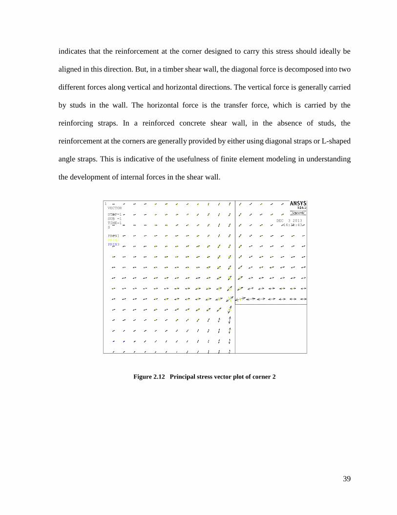
An advantage of finite element modeling is the capability to study the principal stress plot.
Figure 2.12 shows the principal stress vector plot of corner 2 of the model. From this plot, the
direction of principal stress and the type of stress developing at the corner can be identified.
From Figure 2.12, it can be seen that corner 2 is subjected to tensile stress. The length of the
principal stress vector is proportional to its magnitude. In the figure, closer to the corner, the
length of vectors increases. This indicates that the magnitude of stress is much larger closer to
the corner due to stress concentration. The cumulative effect of this stress concentration is the
transfer force. The stress developing at the corner is aligned in an inclined direction. This
39
indicates that the reinforcement at the corner designed to carry this stress should ideally be
aligned in this direction. But, in a timber shear wall, the diagonal force is decomposed into two
different forces along vertical and horizontal directions. The vertical force is generally carried
by studs in the wall. The horizontal force is the transfer force, which is carried by the
reinforcing straps. In a reinforced concrete shear wall, in the absence of studs, the
reinforcement at the corners are generally provided by either using diagonal straps or L-shaped
angle straps. This is indicative of the usefulness of finite element modeling in understanding
the development of internal forces in the shear wall.
Figure 2.12 Principal stress vector plot of corner 2
1
DEC 3 2013
16:31:43
VECTOR
STEP=1
SUB =1
TIME=1
S
PRIN1
PRIN2
PRIN3
40
2.7 Conclusions
In this chapter, the application of four different analytical models to determine the transfer
force around opening corners was explained. Also, a finite element model was developed that
could provide the transfer force at the corners of the opening. The finite element model can
provide results such as the principal stress vectors, which are useful in determining the type of
stress for which reinforcements need to be designed.
The Diekmann model was observed to be most suitable analytical model for determining the
transfer force around window-type openings. The analytical models fail in their application to
walls with multiple openings and door-type openings, which can be analysed using the finite
element model. The coupled-beam analogy is not applicable when there is panel missing above
or below the opening and the Diekmann model is found to over predict the transfer force (Yeh
et al. 2011).
41
Chapter 3: CLT Shear Wall with a Cut-out Opening
Construction of CLT shear walls with openings generally follows two different practices and
each practice has its own design considerations. This chapter focuses on understanding the
reinforcement requirements for the first construction practice in which an opening is cut-out in
the wall. The development of two finite element models used to analyse this construction type
is discussed in this chapter along with the results obtained from finite element analysis. The
first model is a three-dimensional finite element model and the second model is a frame model,
both of which help in analysing the stress distribution around an opening. The second
construction practice of coupled-panel CLT shear walls with openings is discussed in the next
chapter.
3.1 In-plane Behaviour of CLT
It is necessary to study the in-plane behaviour of CLT to understand the type of stress and force
for which reinforcements need to be designed for at the corners of a cut-out opening. The
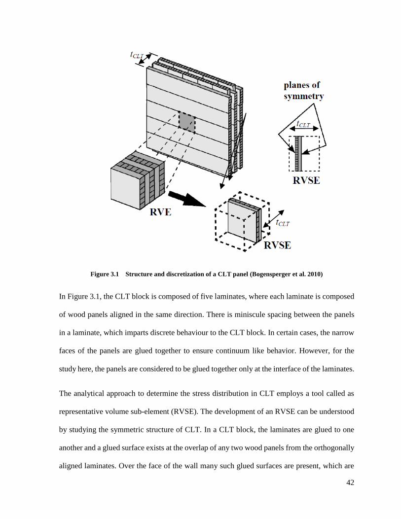
complex structure of CLT is shown in Figure 3.1. The figure shows a CLT block consisting of
five laminates with adjacent laminates aligned orthogonally. This layered arrangement coupled
with the orthotropic nature of wood results in complex behaviour of CLT under the action of
in-plane loads. An analytical approach to explain the stress distribution in a CLT panel was
presented by Bogensperger et al., (2010).
42
Figure 3.1 Structure and discretization of a CLT panel (Bogensperger et al. 2010)
In Figure 3.1, the CLT block is composed of five laminates, where each laminate is composed
of wood panels aligned in the same direction. There is miniscule spacing between the panels
in a laminate, which imparts discrete behaviour to the CLT block. In certain cases, the narrow
faces of the panels are glued together to ensure continuum like behavior. However, for the
study here, the panels are considered to be glued together only at the interface of the laminates.
The analytical approach to determine the stress distribution in CLT employs a tool called as
representative volume sub-element (RVSE). The development of an RVSE can be understood
by studying the symmetric structure of CLT. In a CLT block, the laminates are glued to one
another and a glued surface exists at the overlap of any two wood panels from the orthogonally
aligned laminates. Over the face of the wall many such glued surfaces are present, which are
43
responsible for transfer of force from one laminate to another. The CLT block can be
discretized into smaller elements called as the representative volume elements (RVE) based on
symmetry of the system as shown in Figure 3.1. Each RVE, has planes of symmetry in the
thickness direction as CLT consists of numerous layers. In the case considered here, as there
are five laminates, there are three planes of a symmetry in each RVE. Therefore, the RVE can
be discretized into three smaller repetitive units along these planes of symmetry called as
representative volume sub-elements (RVSE). Each RVSE consists of a single glued surface
and panels associated with that glued surface. The thickness of each RVSE depends on the
laminates it is associated to, the guidelines for which have been outlined by Bogensperger et
al., (2010).
The RVSE is a useful tool in understanding the stress distribution in a CLT block under the
action of an in-plane load. Bogensperger et al., (2010) state that the stress distribution in an
RVSE can be assumed to be constituted of two different mechanisms, a shear mechanism and
a torsion mechanism. These two mechanisms do not exist independently, but their combined
effect helps to analyse the stress distribution in CLT.
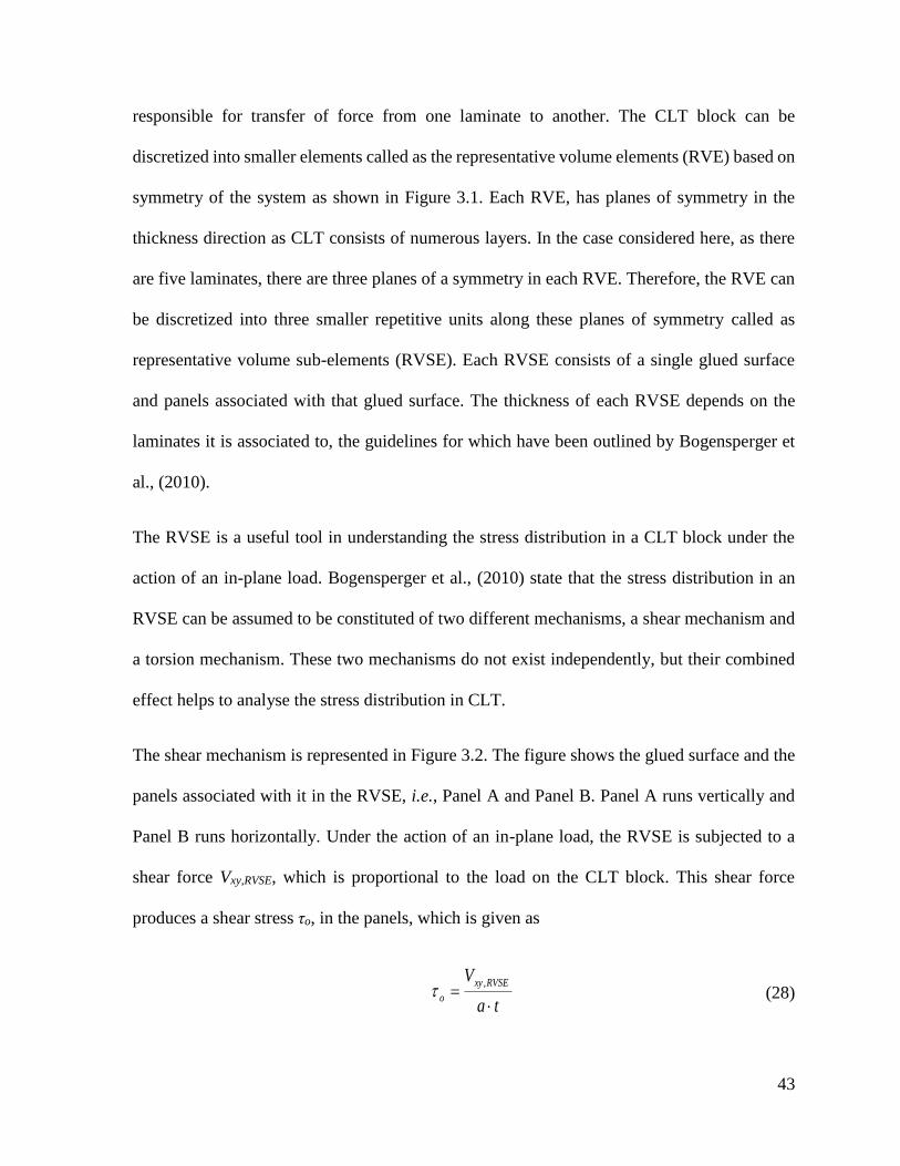
The shear mechanism is represented in Figure 3.2. The figure shows the glued surface and the
panels associated with it in the RVSE, i.e., Panel A and Panel B. Panel A runs vertically and
Panel B runs horizontally. Under the action of an in-plane load, the RVSE is subjected to a
shear force Vxy,RVSE, which is proportional to the load on the CLT block. This shear force
produces a shear stress τo, in the panels, which is given as
ta
V RVSExy
o
,
(28)
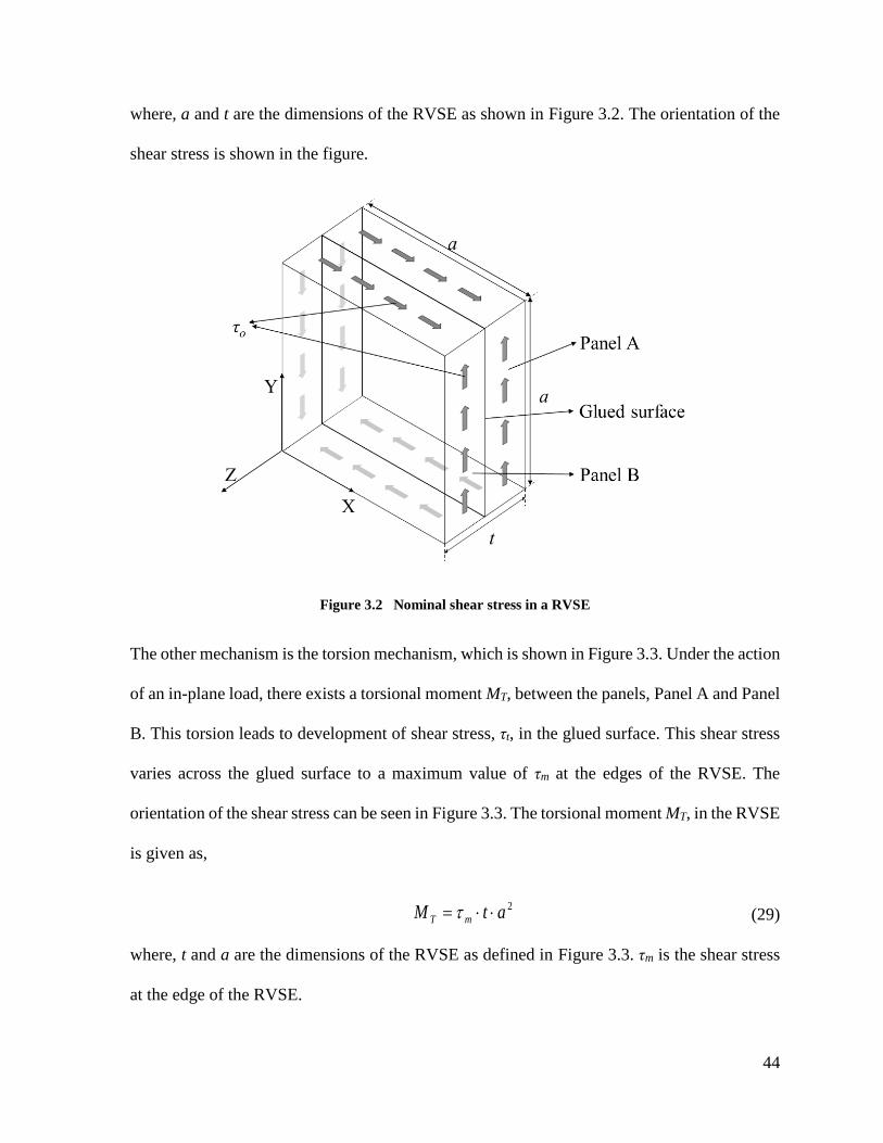
44
where, a and t are the dimensions of the RVSE as shown in Figure 3.2. The orientation of the
shear stress is shown in the figure.
Figure 3.2 Nominal shear stress in a RVSE
The other mechanism is the torsion mechanism, which is shown in Figure 3.3. Under the action
of an in-plane load, there exists a torsional moment MT, between the panels, Panel A and Panel
B. This torsion leads to development of shear stress, τt, in the glued surface. This shear stress
varies across the glued surface to a maximum value of τm at the edges of the RVSE. The
orientation of the shear stress can be seen in Figure 3.3. The torsional moment MT, in the RVSE
is given as,
2atM mT (29)
where, t and a are the dimensions of the RVSE as defined in Figure 3.3. τm is the shear stress
at the edge of the RVSE.

45
Figure 3.3 Torsional shear stress in a RVSE
The combined effect of the two mechanisms described above provides an analytical
approximation of the stress distribution in the RVSE, which is shown in Figure 3.4. Panel A
runs vertically and has vertical free edges along which the shear stress is zero. Similarly, the
shear stress along the horizontal free edges of Panel B is zero. The shear stress along all the
edges by the shear mechanism is τo. The shear stress along all the edges is τm from the torsion
mechanism. The sum of these two mechanisms provides the net shear stress. As the shear stress
at the free edge of the RVSE is zero, the sum of τo and τm is zero. Therefore, the relationship
between the two mechanisms is,
vo (30)
Along the non-free edges of the panels, the shear stress is τv. This shear stress is the sum of the
shear stress from the two mechanisms, i.e., τo and τm. Using Eq. (30), the shear stress at the
non-free edges is computed to be,
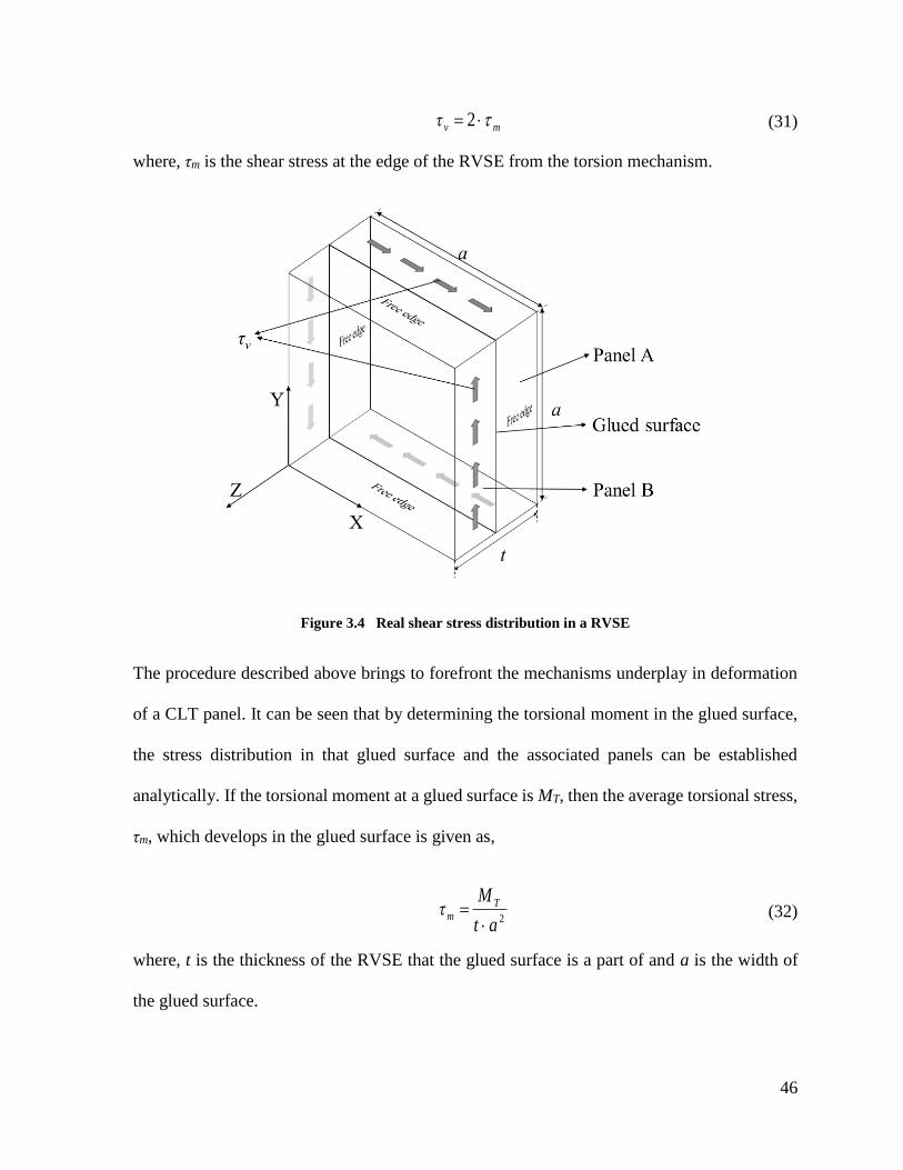
46
mvτ 2 (31)
where, τm is the shear stress at the edge of the RVSE from the torsion mechanism.
Figure 3.4 Real shear stress distribution in a RVSE
The procedure described above brings to forefront the mechanisms underplay in deformation
of a CLT panel. It can be seen that by determining the torsional moment in the glued surface,
the stress distribution in that glued surface and the associated panels can be established
analytically. If the torsional moment at a glued surface is MT, then the average torsional stress,
τm, which develops in the glued surface is given as,
2at
Mτ T
m
(32)
where, t is the thickness of the RVSE that the glued surface is a part of and a is the width of
the glued surface.
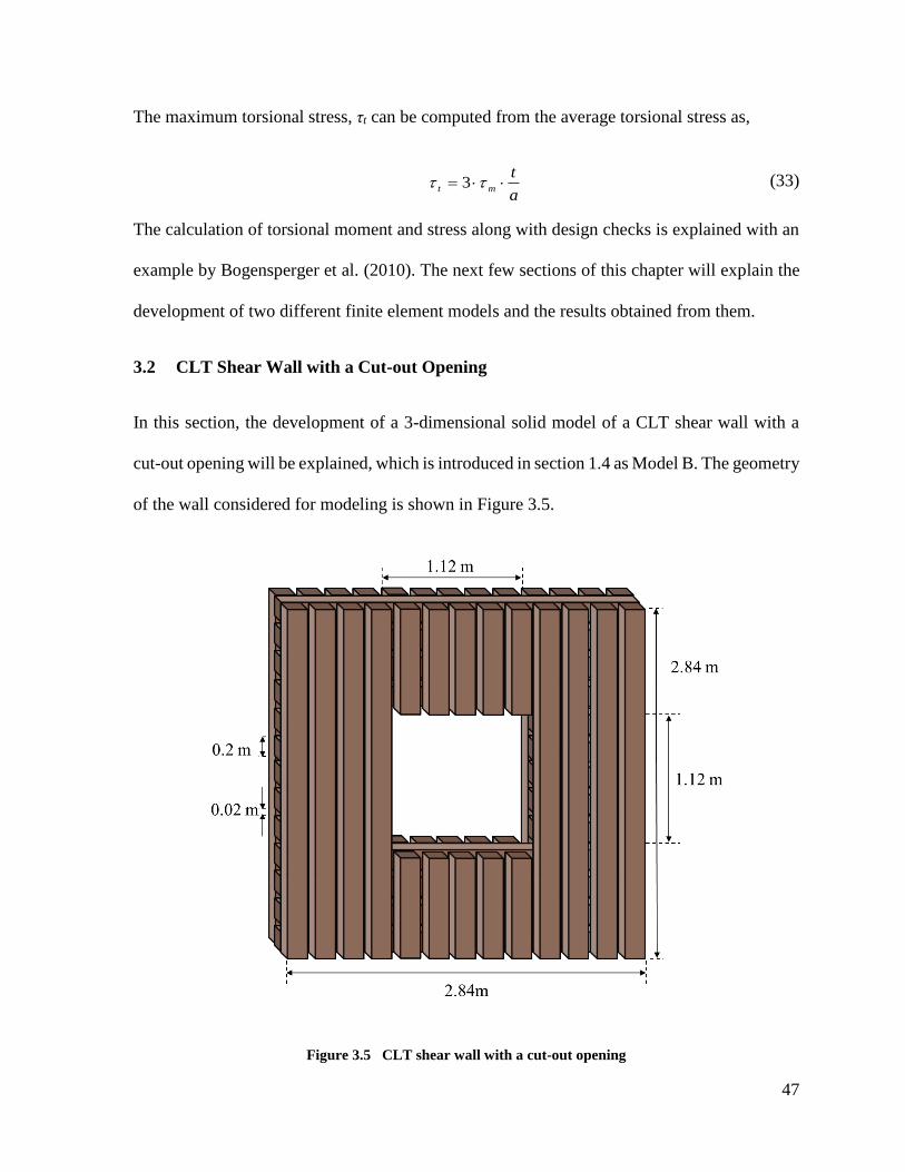
47
The maximum torsional stress, τt can be computed from the average torsional stress as,
a
tmt 3 (33)
The calculation of torsional moment and stress along with design checks is explained with an
example by Bogensperger et al. (2010). The next few sections of this chapter will explain the
development of two different finite element models and the results obtained from them.
3.2 CLT Shear Wall with a Cut-out Opening
In this section, the development of a 3-dimensional solid model of a CLT shear wall with a
cut-out opening will be explained, which is introduced in section 1.4 as Model B. The geometry
of the wall considered for modeling is shown in Figure 3.5.
Figure 3.5 CLT shear wall with a cut-out opening

48
Figure 3.5 shows a square wall of side 2.84m, composed of three laminates with a total
thickness of 0.12m. At the center of the wall, an opening is cut-out of width 1.12m and height
1.12m. Each laminate in the wall is composed of 13 wood panels of width 0.2m, thickness
0.04m and height 2.84m. The spacing between panels in a laminate is assumed to be 0.02m,
which is usually due to engineering limitations or provided intentionally. The spacing between
the panels is limited by functional and aesthetic requirements. In the wall considered here, the
narrow faces of the panels are not considered to be glued together. The three dimensional finite
element model developed in ANSYS for the wall is shown in Figure 3.6.
Figure 3.6 3-dimensional finite element model of a CLT shear wall with a cut-out opening (Model B)
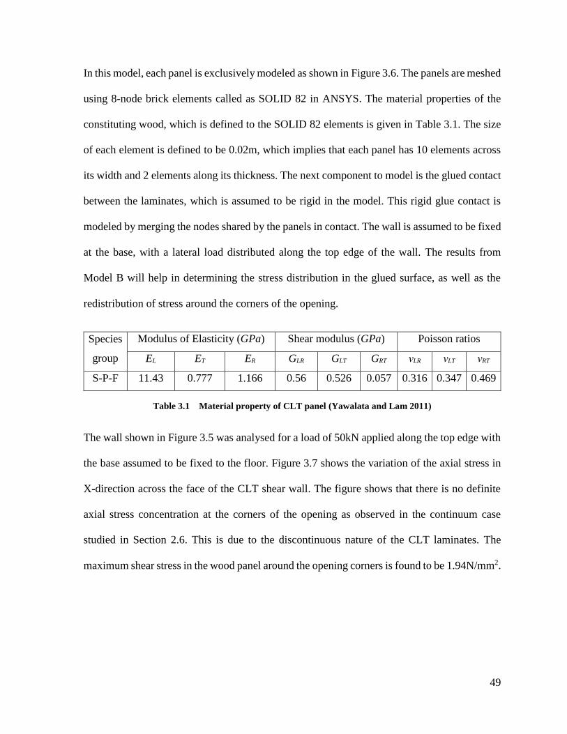
49
In this model, each panel is exclusively modeled as shown in Figure 3.6. The panels are meshed
using 8-node brick elements called as SOLID 82 in ANSYS. The material properties of the
constituting wood, which is defined to the SOLID 82 elements is given in Table 3.1. The size
of each element is defined to be 0.02m, which implies that each panel has 10 elements across
its width and 2 elements along its thickness. The next component to model is the glued contact
between the laminates, which is assumed to be rigid in the model. This rigid glue contact is
modeled by merging the nodes shared by the panels in contact. The wall is assumed to be fixed
at the base, with a lateral load distributed along the top edge of the wall. The results from
Model B will help in determining the stress distribution in the glued surface, as well as the
redistribution of stress around the corners of the opening.
Species
group
Modulus of Elasticity (GPa) Shear modulus (GPa) Poisson ratios
EL ET ER GLR GLT GRT νLR νLT νRT
S-P-F 11.43 0.777 1.166 0.56 0.526 0.057 0.316 0.347 0.469
Table 3.1 Material property of CLT panel (Yawalata and Lam 2011)
The wall shown in Figure 3.5 was analysed for a load of 50kN applied along the top edge with
the base assumed to be fixed to the floor. Figure 3.7 shows the variation of the axial stress in
X-direction across the face of the CLT shear wall. The figure shows that there is no definite
axial stress concentration at the corners of the opening as observed in the continuum case
studied in Section 2.6. This is due to the discontinuous nature of the CLT laminates. The
maximum shear stress in the wood panel around the opening corners is found to be 1.94N/mm2.
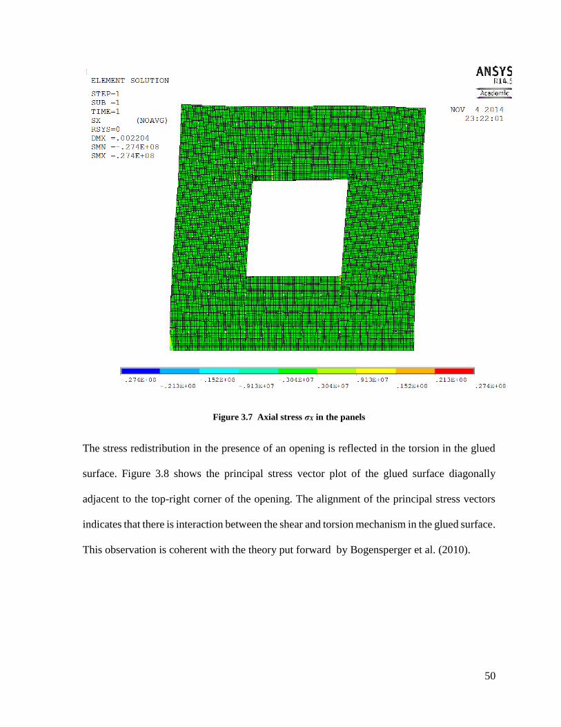
50
Figure 3.7 Axial stress σX in the panels
The stress redistribution in the presence of an opening is reflected in the torsion in the glued
surface. Figure 3.8 shows the principal stress vector plot of the glued surface diagonally
adjacent to the top-right corner of the opening. The alignment of the principal stress vectors
indicates that there is interaction between the shear and torsion mechanism in the glued surface.
This observation is coherent with the theory put forward by Bogensperger et al. (2010).
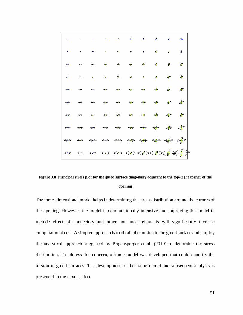
51
Figure 3.8 Principal stress plot for the glued surface diagonally adjacent to the top-right corner of the
opening
The three-dimensional model helps in determining the stress distribution around the corners of
the opening. However, the model is computationally intensive and improving the model to
include effect of connectors and other non-linear elements will significantly increase
computational cost. A simpler approach is to obtain the torsion in the glued surface and employ
the analytical approach suggested by Bogensperger et al. (2010) to determine the stress
distribution. To address this concern, a frame model was developed that could quantify the
torsion in glued surfaces. The development of the frame model and subsequent analysis is
presented in the next section.
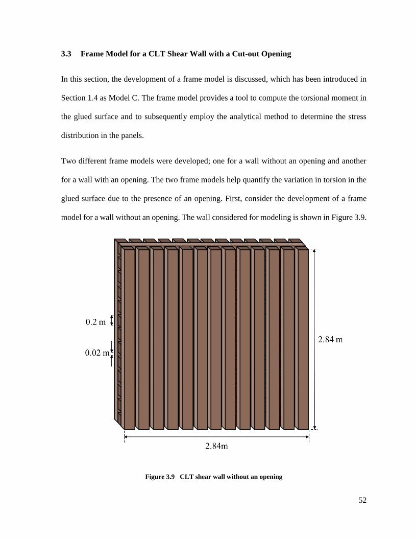
52
3.3 Frame Model for a CLT Shear Wall with a Cut-out Opening
In this section, the development of a frame model is discussed, which has been introduced in
Section 1.4 as Model C. The frame model provides a tool to compute the torsional moment in
the glued surface and to subsequently employ the analytical method to determine the stress
distribution in the panels.
Two different frame models were developed; one for a wall without an opening and another
for a wall with an opening. The two frame models help quantify the variation in torsion in the
glued surface due to the presence of an opening. First, consider the development of a frame
model for a wall without an opening. The wall considered for modeling is shown in Figure 3.9.
Figure 3.9 CLT shear wall without an opening
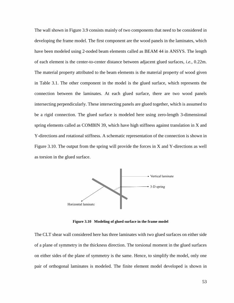
53
The wall shown in Figure 3.9 consists mainly of two components that need to be considered in
developing the frame model. The first component are the wood panels in the laminates, which
have been modeled using 2-noded beam elements called as BEAM 44 in ANSYS. The length
of each element is the center-to-center distance between adjacent glued surfaces, i.e., 0.22m.
The material property attributed to the beam elements is the material property of wood given
in Table 3.1. The other component in the model is the glued surface, which represents the
connection between the laminates. At each glued surface, there are two wood panels
intersecting perpendicularly. These intersecting panels are glued together, which is assumed to
be a rigid connection. The glued surface is modeled here using zero-length 3-dimensional
spring elements called as COMBIN 39, which have high stiffness against translation in X and
Y-directions and rotational stiffness. A schematic representation of the connection is shown in
Figure 3.10. The output from the spring will provide the forces in X and Y-directions as well
as torsion in the glued surface.
Figure 3.10 Modeling of glued surface in the frame model
The CLT shear wall considered here has three laminates with two glued surfaces on either side
of a plane of symmetry in the thickness direction. The torsional moment in the glued surfaces
on either sides of the plane of symmetry is the same. Hence, to simplify the model, only one
pair of orthogonal laminates is modeled. The finite element model developed is shown in
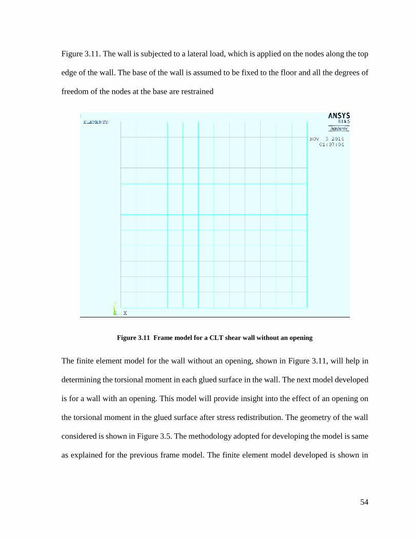
54
Figure 3.11. The wall is subjected to a lateral load, which is applied on the nodes along the top
edge of the wall. The base of the wall is assumed to be fixed to the floor and all the degrees of
freedom of the nodes at the base are restrained
Figure 3.11 Frame model for a CLT shear wall without an opening
The finite element model for the wall without an opening, shown in Figure 3.11, will help in
determining the torsional moment in each glued surface in the wall. The next model developed
is for a wall with an opening. This model will provide insight into the effect of an opening on
the torsional moment in the glued surface after stress redistribution. The geometry of the wall
considered is shown in Figure 3.5. The methodology adopted for developing the model is same
as explained for the previous frame model. The finite element model developed is shown in

55
Figure 3.12. The loading and boundary conditions are same as applied on the model shown in
Figure 3.11.
The torsional moment at each glued surface in the wall can be obtained from the model using
the COMBIN39 spring elements. A comparison of the torsional moment at each glued surface
between the two frame models will provide an insight into the effect of the opening. The stress
distribution in the glued surface and across the face of the wall can now be determined using
Eq. (31), Eq. (32) and Eq. (33). Failure in the glued surface and wood panels is brittle in nature
and damage at these locations need to be avoided.
Figure 3.12 Frame model for a CLT shear wall with a cut-out opening (Model C)

56
3.4 Results from the Frame Models (Model C)
The frame models discussed in Section 3.3 provide a tool to determine the torsion in the glued
surfaces. In this section, the results from the analysis of the two frame models developed is
presented and the shear stress obtained is compared to the value obtained using the three-
dimensional finite element model. The three dimensional finite element model was subjected
to a lateral load of 50kN. As the frame model considers only half the thickness of the wall in
analysis, the load applied also needs to be halved. Therefore, a lateral load of 25kN is applied
along the top edge of both the frame models and the torsional moment in each glued surface is
obtained.
First, the results from analysis of the frame model for a wall without an opening is presented.
Figure 3.13 shows the torsion in each glued surface across the face of the wall between two
CLT laminates for a lateral load of 25kN. The glued surfaces at the base of the wall have no
torsion due to the fixed boundary condition assigned to the model. The torsional moment is
evenly distributed in the glued surfaces in the middle due to even stress distribution. The
torsion in glued surfaces towards the periphery of the wall decreases due to boundary effects.

57
Figure 3.13 Torsion (Nm) in each glued surface of a CLT shear wall
The frame model with an opening provides the torsional moment in each glued surface, which
is shown in Figure 3.14. The load and boundary conditions on the wall are same as in the
previous case. The torsional moment is not equally distributed over the face of the wall due to
stress redistribution around the opening. The glued surfaces along the free edges of the opening
experience significantly lower torsional moment due to the free boundary condition. The lower
torsion in these glued surfaces results in increased torsion in the glued surfaces adjacent to
them. This effect is most profound in the glued surfaces located at the corners of the opening,
which have been highlighted in red in Figure 3.14.
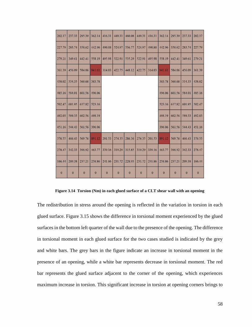
58
Figure 3.14 Torsion (Nm) in each glued surface of a CLT shear wall with an opening
The redistribution in stress around the opening is reflected in the variation in torsion in each
glued surface. Figure 3.15 shows the difference in torsional moment experienced by the glued
surfaces in the bottom left quarter of the wall due to the presence of the opening. The difference
in torsional moment in each glued surface for the two cases studied is indicated by the grey
and white bars. The grey bars in the figure indicate an increase in torsional moment in the
presence of an opening, while a white bar represents decrease in torsional moment. The red
bar represents the glued surface adjacent to the corner of the opening, which experiences
maximum increase in torsion. This significant increase in torsion at opening corners brings to
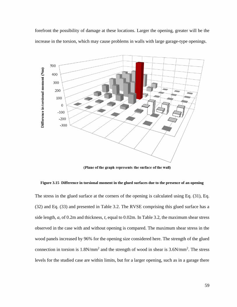
59
forefront the possibility of damage at these locations. Larger the opening, greater will be the
increase in the torsion, which may cause problems in walls with large garage-type openings.
Figure 3.15 Difference in torsional moment in the glued surfaces due to the presence of an opening
The stress in the glued surface at the corners of the opening is calculated using Eq. (31), Eq.
(32) and Eq. (33) and presented in Table 3.2. The RVSE comprising this glued surface has a
side length, a, of 0.2m and thickness, t, equal to 0.02m. In Table 3.2, the maximum shear stress
observed in the case with and without opening is compared. The maximum shear stress in the
wood panels increased by 96% for the opening size considered here. The strength of the glued
connection in torsion is 1.8N/mm2 and the strength of wood in shear is 3.6N/mm2. The stress
levels for the studied case are within limits, but for a larger opening, such as in a garage there
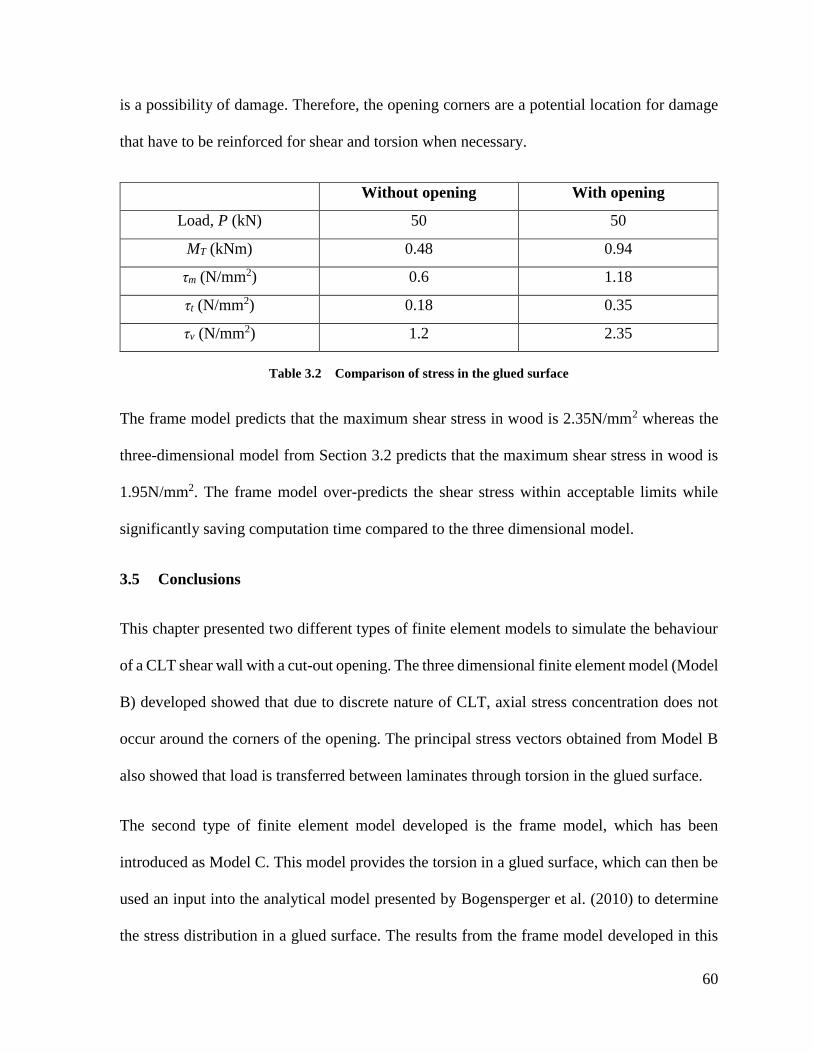
60
is a possibility of damage. Therefore, the opening corners are a potential location for damage
that have to be reinforced for shear and torsion when necessary.
Without opening With opening
Load, P (kN) 50 50
MT (kNm) 0.48 0.94
τm (N/mm2) 0.6 1.18
τt (N/mm2) 0.18 0.35
τv (N/mm2) 1.2 2.35
Table 3.2 Comparison of stress in the glued surface
The frame model predicts that the maximum shear stress in wood is 2.35N/mm2 whereas the
three-dimensional model from Section 3.2 predicts that the maximum shear stress in wood is
1.95N/mm2. The frame model over-predicts the shear stress within acceptable limits while
significantly saving computation time compared to the three dimensional model.
3.5 Conclusions
This chapter presented two different types of finite element models to simulate the behaviour
of a CLT shear wall with a cut-out opening. The three dimensional finite element model (Model
B) developed showed that due to discrete nature of CLT, axial stress concentration does not
occur around the corners of the opening. The principal stress vectors obtained from Model B
also showed that load is transferred between laminates through torsion in the glued surface.
The second type of finite element model developed is the frame model, which has been
introduced as Model C. This model provides the torsion in a glued surface, which can then be
used an input into the analytical model presented by Bogensperger et al. (2010) to determine
the stress distribution in a glued surface. The results from the frame model developed in this
61
chapter showed that there is stress redistribution as indicated by increase in torsion in the glued
surface adjacent to opening corners. The subsequent calculation of stress also showed that there
is a possibility of shear failure in wood around the opening corners. The results though are not
conclusive as the stress values have been obtained using an analytical model. Experimental
testing of such wall set-ups need to be conducted in future to understand the reinforcement
requirements in more detail. Nonetheless, the results from the finite element models indicate
the type of stresses that develop at the corners of the opening for which reinforcements have
to be designed.
62
Chapter 4: Coupled-Panel CLT Shear Walls
In this chapter, the focus is on CLT shear walls with coupled-panels around openings, which
is a commonly observed construction practice in North America. The analysis of this
construction practice is carried out using a finite element model calibrated to experimental
data, which has been introduced in section 1.4 as Model D. This chapter explains the
development of the finite element model and the results obtained from it. This construction
approach is popular because of three reasons. First, the use of smaller panels to form a wall
with an opening reduces the wastage of material, which amounts to substantial savings in large-
scale projects. Secondly, the process of cutting an opening in a CLT shear wall, which was
described in the previous chapter, is difficult and requires skilled labour and expensive tools
for cutting. Thirdly, by coupling the panels together using metal connectors, the wall has an
additional source of ductility. Ductility in timber walls has been observed to significantly
increase the reliability and robustness of the walls (Kirkegaard et al. 2011) making them more
viable for use in high seismic zones.
In the coupled-wall construction practice, under the action of a lateral load, the deformation in
the wall is mainly concentrated to the connectors. Due to this characteristic, the torsional
mechanism and related failure in CLT discussed in the previous chapter will not be of
significant concern. In the next section, the development of an experimentally calibrated finite
element model will be discussed. The model development procedure will be first validated by
simulating an experiment from literature.

63
4.1 Modeling a Coupled-Panel CLT Shear Wall
In this section, the development of a finite element model for a coupled-panel CLT shear wall
will be discussed. This model focuses on simulating the connection between the panels and
establishing a modeling procedure. The wall considered for modeling is shown in Figure 4.1,
which has a dimension of 2.95m x 2.95m and is composed of a 5-layered CLT panel with a
total thickness of 85mm. The wall consists of two panels connected together using a half lap
joint. The wall panel is connected to the floor of the set-up by two hold-downs at the edges of
the wall and four angle brackets as shown in the figure. This test set up was analysed by Gavric
et al. (2012) to study the seismic performance of the CLT shear walls. However, the results
from the test have been used here to validate the modeling approach by conducting a push-
over analysis.
Figure 4.1 Coupled-panel CLT shear wall (Gavric et al. 2012)
64
The CLT shear wall shown in Figure 4.1 has different components, such as the CLT wall panel,
wall-to-floor connection, panel-to-panel connection, wall-to-floor contact and panel-to-panel
contact. These components have been modeled explicitly and calibrated to experimentally
determined behaviour. In the next few sections of this chapter, the modeling of each of these
components will be explained.
4.2 Modeling the CLT Panels
Under the action of a lateral load, the CLT panels in the wall undergo only in-plane
deformation. Hence, plane stress quadrilateral elements called as PLANE42 were used to
model the CLT panels. The CLT panel is composed of laminates, which exhibit orthotropic
material behaviour that has been presented previously in Table 3.1. This material behaviour is
incorporated into the model by homogenizing the material property over the numerous layers.
The CLT Handbook (Gagnon and Popovski 2011) describes a procedure for homogenization
of the material property using the concept of k-factors from composite theory. Figure 4.2 and
Figure 4.3 present snippets from the CLT handbook, which explain the calculation of the k-
factors and the effective homogenized properties of the CLT panel. k3 and k4 are the k-factors
that have to be computed in this case for determining the effective panel properties under the
action of an in-plane load. In the equations for the k-factors, Eo and E90 are the moduli of
elasticity in the lateral and longitudinal directions. ai is the thickness of the ith laminate in the
CLT board. The homogenized material property for the CLT laminate manufactured by
Structurlam (Structurlam n.d.) is presented in Table 4.1, which is the material model input for
the plane stress elements.
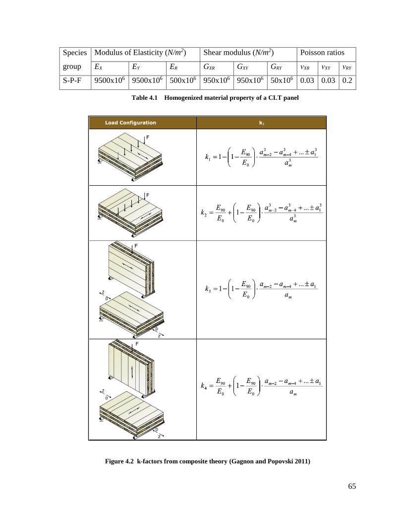
65
Species
group
Modulus of Elasticity (N/m2) Shear modulus (N/m2) Poisson ratios
EX EY ER GXR GXY GRY νXR νXY νRY
S-P-F 9500x106 9500x106 500x106 950x106 950x106 50x106 0.03 0.03 0.2
Table 4.1 Homogenized material property of a CLT panel
Figure 4.2 k-factors from composite theory (Gagnon and Popovski 2011)
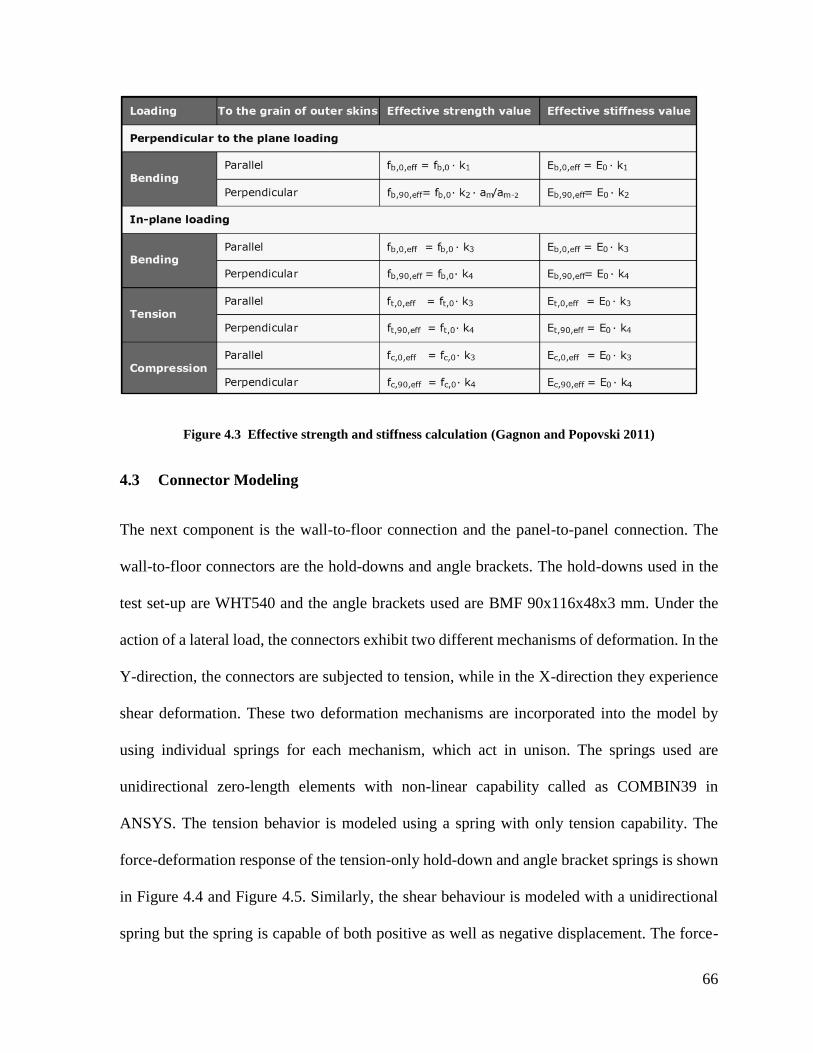
66
Figure 4.3 Effective strength and stiffness calculation (Gagnon and Popovski 2011)
4.3 Connector Modeling
The next component is the wall-to-floor connection and the panel-to-panel connection. The
wall-to-floor connectors are the hold-downs and angle brackets. The hold-downs used in the
test set-up are WHT540 and the angle brackets used are BMF 90x116x48x3 mm. Under the
action of a lateral load, the connectors exhibit two different mechanisms of deformation. In the
Y-direction, the connectors are subjected to tension, while in the X-direction they experience
shear deformation. These two deformation mechanisms are incorporated into the model by
using individual springs for each mechanism, which act in unison. The springs used are
unidirectional zero-length elements with non-linear capability called as COMBIN39 in
ANSYS. The tension behavior is modeled using a spring with only tension capability. The
force-deformation response of the tension-only hold-down and angle bracket springs is shown
in Figure 4.4 and Figure 4.5. Similarly, the shear behaviour is modeled with a unidirectional
spring but the spring is capable of both positive as well as negative displacement. The force-
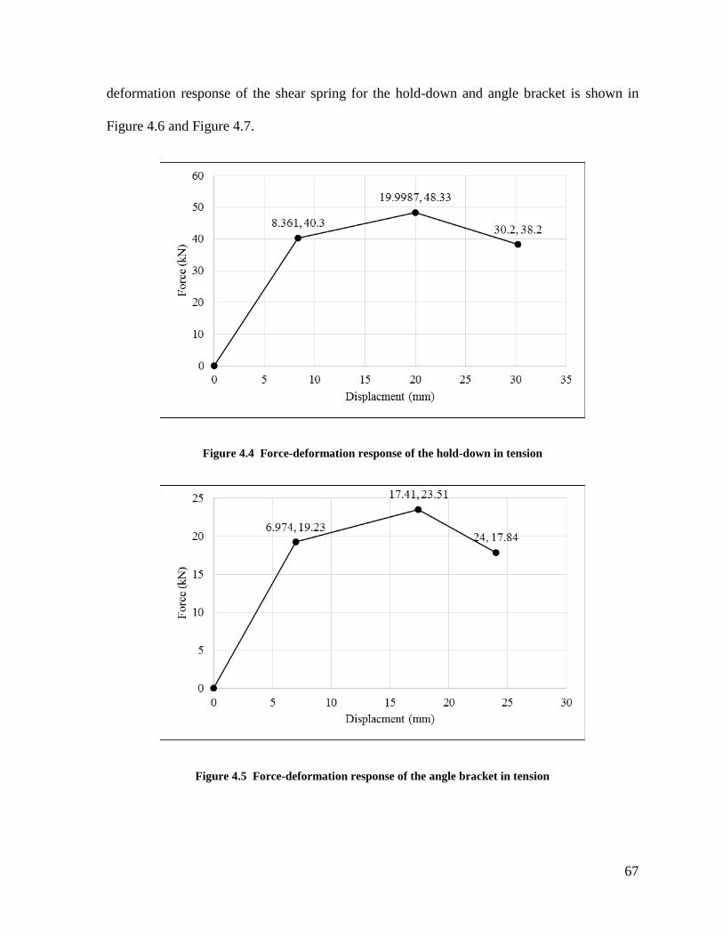
67
deformation response of the shear spring for the hold-down and angle bracket is shown in
Figure 4.6 and Figure 4.7.
Figure 4.4 Force-deformation response of the hold-down in tension
Figure 4.5 Force-deformation response of the angle bracket in tension

68
Figure 4.6 Force-deformation response of the hold-down in shear
Figure 4.7 Force-deformation response of the angle bracket in shear
The panels are joined together with a half-lap joint with an overlap length of 50mm using self-
tapping screws type HBSΦ8x80mm at 150mm c/c spacing. The screws in this joint were
modeled using COMBIN39 springs with unidirectional behaviour. Each screw was modeled
using a pair of zero-length springs, one for deformation in X-direction and the other for
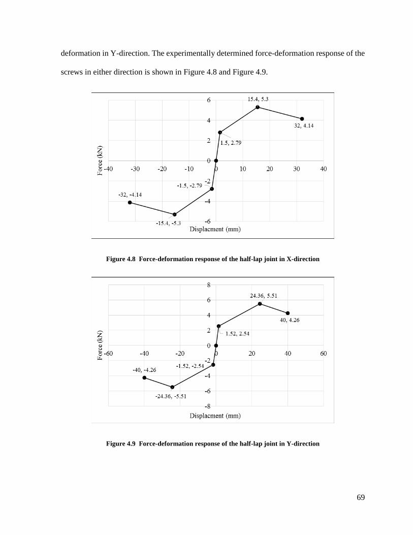
69
deformation in Y-direction. The experimentally determined force-deformation response of the
screws in either direction is shown in Figure 4.8 and Figure 4.9.
Figure 4.8 Force-deformation response of the half-lap joint in X-direction
Figure 4.9 Force-deformation response of the half-lap joint in Y-direction
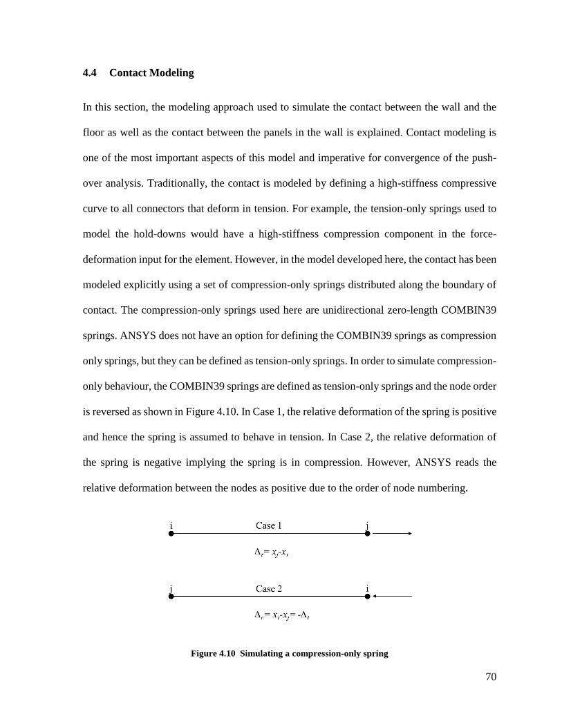
70
4.4 Contact Modeling
In this section, the modeling approach used to simulate the contact between the wall and the
floor as well as the contact between the panels in the wall is explained. Contact modeling is
one of the most important aspects of this model and imperative for convergence of the push-
over analysis. Traditionally, the contact is modeled by defining a high-stiffness compressive
curve to all connectors that deform in tension. For example, the tension-only springs used to
model the hold-downs would have a high-stiffness compression component in the force-
deformation input for the element. However, in the model developed here, the contact has been
modeled explicitly using a set of compression-only springs distributed along the boundary of
contact. The compression-only springs used here are unidirectional zero-length COMBIN39
springs. ANSYS does not have an option for defining the COMBIN39 springs as compression
only springs, but they can be defined as tension-only springs. In order to simulate compression-
only behaviour, the COMBIN39 springs are defined as tension-only springs and the node order
is reversed as shown in Figure 4.10. In Case 1, the relative deformation of the spring is positive
and hence the spring is assumed to behave in tension. In Case 2, the relative deformation of
the spring is negative implying the spring is in compression. However, ANSYS reads the
relative deformation between the nodes as positive due to the order of node numbering.
Figure 4.10 Simulating a compression-only spring
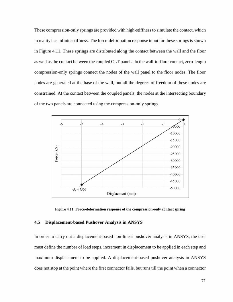
71
These compression-only springs are provided with high-stiffness to simulate the contact, which
in reality has infinite stiffness. The force-deformation response input for these springs is shown
in Figure 4.11. These springs are distributed along the contact between the wall and the floor
as well as the contact between the coupled CLT panels. In the wall-to-floor contact, zero-length
compression-only springs connect the nodes of the wall panel to the floor nodes. The floor
nodes are generated at the base of the wall, but all the degrees of freedom of these nodes are
constrained. At the contact between the coupled panels, the nodes at the intersecting boundary
of the two panels are connected using the compression-only springs.
Figure 4.11 Force-deformation response of the compression-only contact spring
4.5 Displacement-based Pushover Analysis in ANSYS
In order to carry out a displacement-based non-linear pushover analysis in ANSYS, the user
must define the number of load steps, increment in displacement to be applied in each step and
maximum displacement to be applied. A displacement-based pushover analysis in ANSYS
does not stop at the point where the first connector fails, but runs till the point when a connector

72
experiences negative force for a positive displacement. Therefore, the user must always check
back the solution obtained to determine the exact load step at which the wall failed. For the
test set-up considered here, a maximum displacement of 35mm is applied. Figure 4.12 shows
the finite element model that has been developed to simulate the test set-up shown in Figure
4.1 under the action of a lateral load.
Figure 4.12 Finite element model of the test set-up by Gavric et al. (2012)
The deformation of the wall is shown in Figure 4.13. The shear deformation between the
coupled-panels is clearly visible in the figure. The pushover curve obtained through the
simulation is shown in Figure 4.14. The force-deformation response obtained matches to the
experimental response observed by Gavric et al. (2012). This indicates that the modeling
procedure adopted here appropriate and can be extended to simulate the behaviour of a
coupled-panel CLT shear wall with an opening.
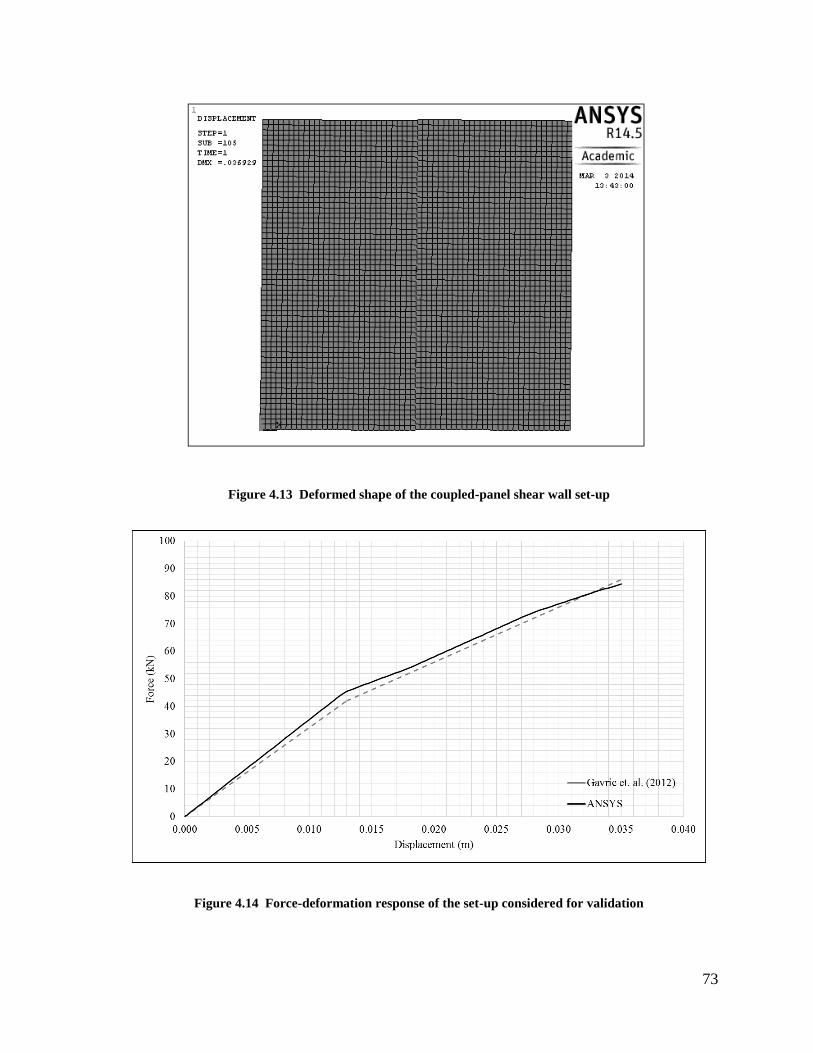
73
Figure 4.13 Deformed shape of the coupled-panel shear wall set-up
Figure 4.14 Force-deformation response of the set-up considered for validation
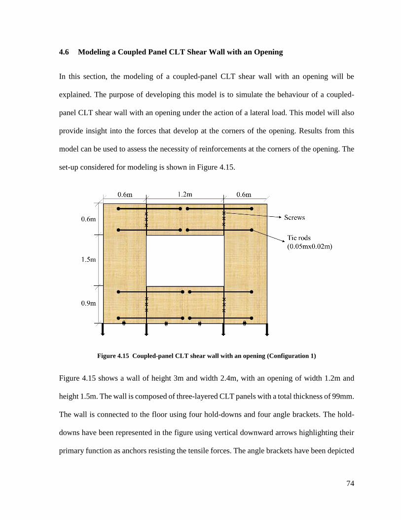
74
4.6 Modeling a Coupled Panel CLT Shear Wall with an Opening
In this section, the modeling of a coupled-panel CLT shear wall with an opening will be
explained. The purpose of developing this model is to simulate the behaviour of a coupled-
panel CLT shear wall with an opening under the action of a lateral load. This model will also
provide insight into the forces that develop at the corners of the opening. Results from this
model can be used to assess the necessity of reinforcements at the corners of the opening. The
set-up considered for modeling is shown in Figure 4.15.
Figure 4.15 Coupled-panel CLT shear wall with an opening (Configuration 1)
Figure 4.15 shows a wall of height 3m and width 2.4m, with an opening of width 1.2m and
height 1.5m. The wall is composed of three-layered CLT panels with a total thickness of 99mm.
The wall is connected to the floor using four hold-downs and four angle brackets. The hold-
downs have been represented in the figure using vertical downward arrows highlighting their
primary function as anchors resisting the tensile forces. The angle brackets have been depicted
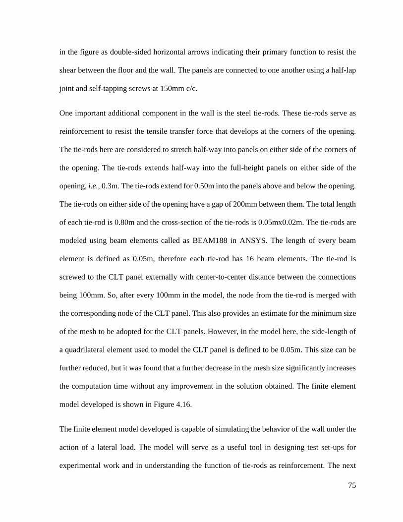
75
in the figure as double-sided horizontal arrows indicating their primary function to resist the
shear between the floor and the wall. The panels are connected to one another using a half-lap
joint and self-tapping screws at 150mm c/c.
One important additional component in the wall is the steel tie-rods. These tie-rods serve as
reinforcement to resist the tensile transfer force that develops at the corners of the opening.
The tie-rods here are considered to stretch half-way into panels on either side of the corners of
the opening. The tie-rods extends half-way into the full-height panels on either side of the
opening, i.e., 0.3m. The tie-rods extend for 0.50m into the panels above and below the opening.
The tie-rods on either side of the opening have a gap of 200mm between them. The total length
of each tie-rod is 0.80m and the cross-section of the tie-rods is 0.05mx0.02m. The tie-rods are
modeled using beam elements called as BEAM188 in ANSYS. The length of every beam
element is defined as 0.05m, therefore each tie-rod has 16 beam elements. The tie-rod is
screwed to the CLT panel externally with center-to-center distance between the connections
being 100mm. So, after every 100mm in the model, the node from the tie-rod is merged with
the corresponding node of the CLT panel. This also provides an estimate for the minimum size
of the mesh to be adopted for the CLT panels. However, in the model here, the side-length of
a quadrilateral element used to model the CLT panel is defined to be 0.05m. This size can be
further reduced, but it was found that a further decrease in the mesh size significantly increases
the computation time without any improvement in the solution obtained. The finite element
model developed is shown in Figure 4.16.
The finite element model developed is capable of simulating the behavior of the wall under the
action of a lateral load. The model will serve as a useful tool in designing test set-ups for
experimental work and in understanding the function of tie-rods as reinforcement. The next
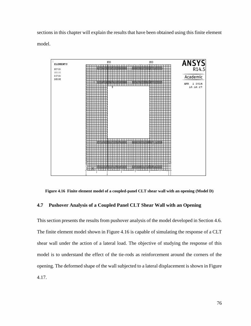
76
sections in this chapter will explain the results that have been obtained using this finite element
model.
Figure 4.16 Finite element model of a coupled-panel CLT shear wall with an opening (Model D)
4.7 Pushover Analysis of a Coupled Panel CLT Shear Wall with an Opening
This section presents the results from pushover analysis of the model developed in Section 4.6.
The finite element model shown in Figure 4.16 is capable of simulating the response of a CLT
shear wall under the action of a lateral load. The objective of studying the response of this
model is to understand the effect of the tie-rods as reinforcement around the corners of the
opening. The deformed shape of the wall subjected to a lateral displacement is shown in Figure
4.17.
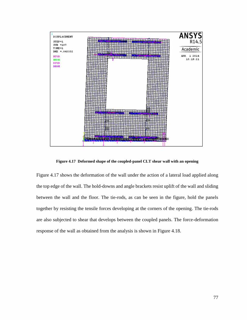
77
Figure 4.17 Deformed shape of the coupled-panel CLT shear wall with an opening
Figure 4.17 shows the deformation of the wall under the action of a lateral load applied along
the top edge of the wall. The hold-downs and angle brackets resist uplift of the wall and sliding
between the wall and the floor. The tie-rods, as can be seen in the figure, hold the panels
together by resisting the tensile forces developing at the corners of the opening. The tie-rods
are also subjected to shear that develops between the coupled panels. The force-deformation
response of the wall as obtained from the analysis is shown in Figure 4.18.
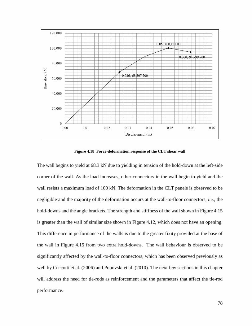
78
Figure 4.18 Force-deformation response of the CLT shear wall
The wall begins to yield at 68.3 kN due to yielding in tension of the hold-down at the left-side
corner of the wall. As the load increases, other connectors in the wall begin to yield and the
wall resists a maximum load of 100 kN. The deformation in the CLT panels is observed to be
negligible and the majority of the deformation occurs at the wall-to-floor connectors, i.e., the
hold-downs and the angle brackets. The strength and stiffness of the wall shown in Figure 4.15
is greater than the wall of similar size shown in Figure 4.12, which does not have an opening.
This difference in performance of the walls is due to the greater fixity provided at the base of
the wall in Figure 4.15 from two extra hold-downs. The wall behaviour is observed to be
significantly affected by the wall-to-floor connectors, which has been observed previously as
well by Ceccotti et al. (2006) and Popovski et al. (2010). The next few sections in this chapter
will address the need for tie-rods as reinforcement and the parameters that affect the tie-rod
performance.
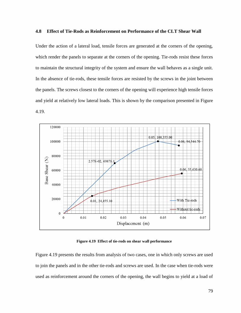
79
4.8 Effect of Tie-Rods as Reinforcement on Performance of the CLT Shear Wall
Under the action of a lateral load, tensile forces are generated at the corners of the opening,
which render the panels to separate at the corners of the opening. Tie-rods resist these forces
to maintain the structural integrity of the system and ensure the wall behaves as a single unit.
In the absence of tie-rods, these tensile forces are resisted by the screws in the joint between
the panels. The screws closest to the corners of the opening will experience high tensile forces
and yield at relatively low lateral loads. This is shown by the comparison presented in Figure
4.19.
Figure 4.19 Effect of tie-rods on shear wall performance
Figure 4.19 presents the results from analysis of two cases, one in which only screws are used
to join the panels and in the other tie-rods and screws are used. In the case when tie-rods were
used as reinforcement around the corners of the opening, the wall begins to yield at a load of
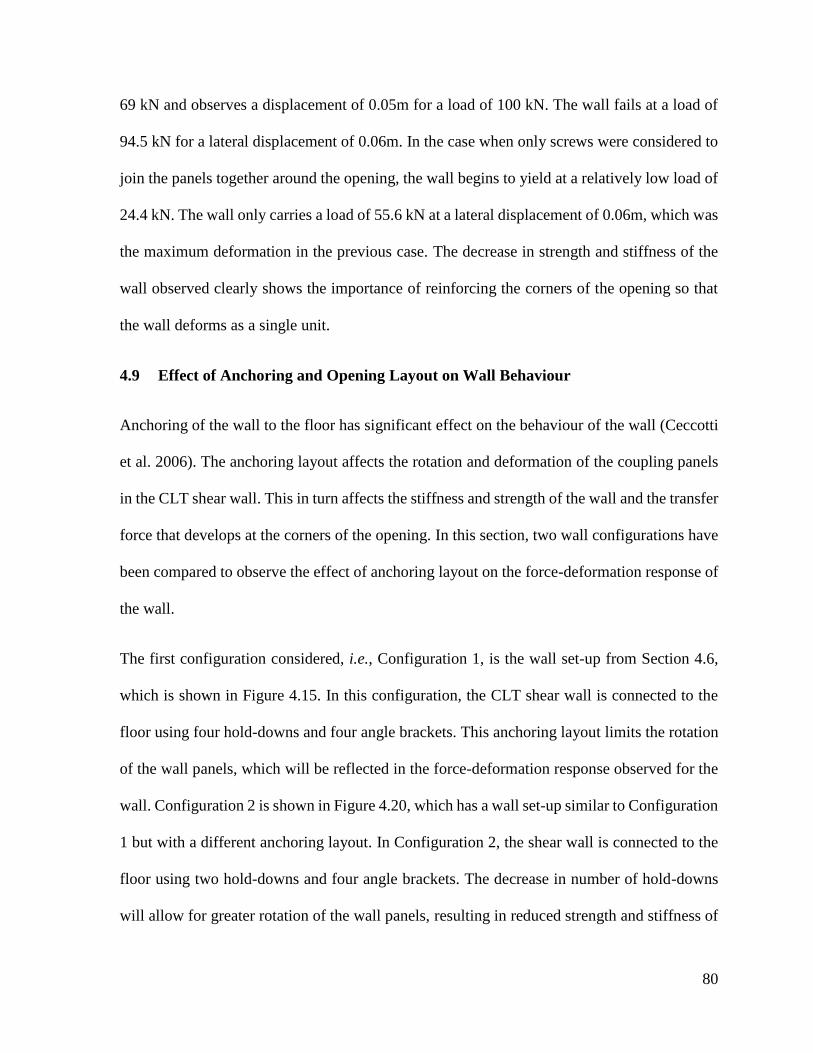
80
69 kN and observes a displacement of 0.05m for a load of 100 kN. The wall fails at a load of
94.5 kN for a lateral displacement of 0.06m. In the case when only screws were considered to
join the panels together around the opening, the wall begins to yield at a relatively low load of
24.4 kN. The wall only carries a load of 55.6 kN at a lateral displacement of 0.06m, which was
the maximum deformation in the previous case. The decrease in strength and stiffness of the
wall observed clearly shows the importance of reinforcing the corners of the opening so that
the wall deforms as a single unit.
4.9 Effect of Anchoring and Opening Layout on Wall Behaviour
Anchoring of the wall to the floor has significant effect on the behaviour of the wall (Ceccotti
et al. 2006). The anchoring layout affects the rotation and deformation of the coupling panels
in the CLT shear wall. This in turn affects the stiffness and strength of the wall and the transfer
force that develops at the corners of the opening. In this section, two wall configurations have
been compared to observe the effect of anchoring layout on the force-deformation response of
the wall.
The first configuration considered, i.e., Configuration 1, is the wall set-up from Section 4.6,
which is shown in Figure 4.15. In this configuration, the CLT shear wall is connected to the
floor using four hold-downs and four angle brackets. This anchoring layout limits the rotation
of the wall panels, which will be reflected in the force-deformation response observed for the
wall. Configuration 2 is shown in Figure 4.20, which has a wall set-up similar to Configuration
1 but with a different anchoring layout. In Configuration 2, the shear wall is connected to the
floor using two hold-downs and four angle brackets. The decrease in number of hold-downs
will allow for greater rotation of the wall panels, resulting in reduced strength and stiffness of
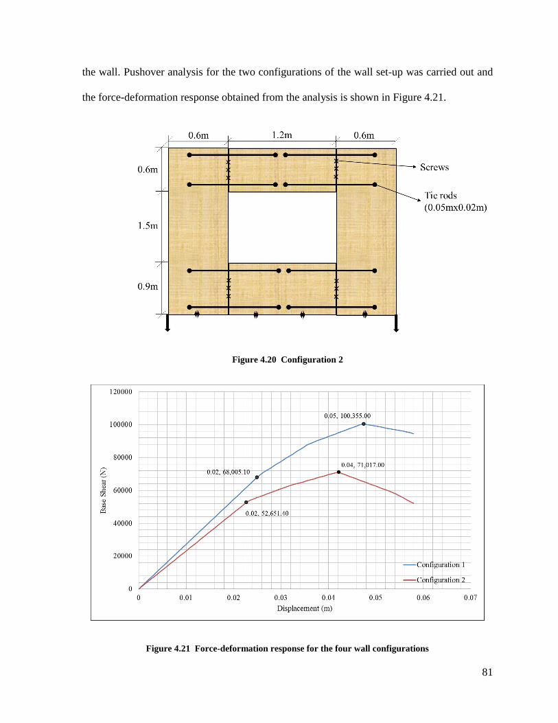
81
the wall. Pushover analysis for the two configurations of the wall set-up was carried out and
the force-deformation response obtained from the analysis is shown in Figure 4.21.
Figure 4.20 Configuration 2
Figure 4.21 Force-deformation response for the four wall configurations
82
Figure 4.21 shows that the anchoring layout significantly affects the strength and stiffness of
the CLT shear wall. Configuration 1 has a yield strength of 68kN and maximum strength of
100 kN, whereas Configuration 2 has a yield strength of 52 kN and a maximum strength of 72
kN. The increase in strength and stiffness of Configuration 1 compared to Configuration 2 is
due to the reduced rotation of the CLT wall panels. The two additional hold-downs in
Configuration 1 can resist greater uplift and shear forces and reduce the deformation in the
anchors, which in turn leads to reduced rotation and displacement of the wall panels.
The study in this section shows that the anchoring layout plays a significant role in determining
the maximum base shear the wall will be subjected to. As the transfer force is a function of this
base shear, the design transfer force will depend on the anchoring layout. Moreover, the
anchoring layout will affect the shear force that develops between the panels, which will be
resisted by the tie-rods and panel-to-panel connectors.
4.10 Design Transfer Force from the Diekmann Model and Finite Element Models
In this section, the effect of anchoring layout on the design transfer force is studied. Also, the
Diekmann model has been used to determine the design transfer force in the tie-rods to assess
its applicability for the two wall configurations introduced in the previous section.
The Diekmann method provides the transfer force, FT, which develops at the edge of the
opening. The tie-rod however, is located at an edge-distance, e, from the free-edge of the
opening as shown in Figure 4.22. Therefore, the transfer force obtained using the Diekmann
model has to be corrected for this edge-distance to determine the force in the tie-rods, FTR.
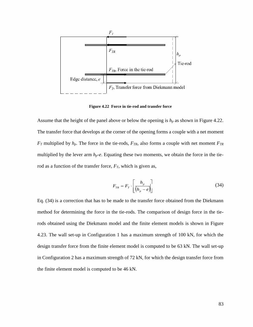
83
Figure 4.22 Force in tie-rod and transfer force
Assume that the height of the panel above or below the opening is hp as shown in Figure 4.22.
The transfer force that develops at the corner of the opening forms a couple with a net moment
FT multiplied by hp. The force in the tie-rods, FTR, also forms a couple with net moment FTR
multiplied by the lever arm hp-e. Equating these two moments, we obtain the force in the tie-
rod as a function of the transfer force, FT, which is given as,
eh
hFF
p
p
TTR (34)
Eq. (34) is a correction that has to be made to the transfer force obtained from the Diekmann
method for determining the force in the tie-rods. The comparison of design force in the tie-
rods obtained using the Diekmann model and the finite element models is shown in Figure
4.23. The wall set-up in Configuration 1 has a maximum strength of 100 kN, for which the
design transfer force from the finite element model is computed to be 63 kN. The wall set-up
in Configuration 2 has a maximum strength of 72 kN, for which the design transfer force from
the finite element model is computed to be 46 kN.
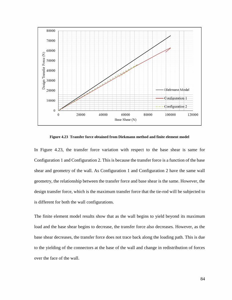
84
Figure 4.23 Transfer force obtained from Diekmann method and finite element model
In Figure 4.23, the transfer force variation with respect to the base shear is same for
Configuration 1 and Configuration 2. This is because the transfer force is a function of the base
shear and geometry of the wall. As Configuration 1 and Configuration 2 have the same wall
geometry, the relationship between the transfer force and base shear is the same. However, the
design transfer force, which is the maximum transfer force that the tie-rod will be subjected to
is different for both the wall configurations.
The finite element model results show that as the wall begins to yield beyond its maximum
load and the base shear begins to decrease, the transfer force also decreases. However, as the
base shear decreases, the transfer force does not trace back along the loading path. This is due
to the yielding of the connectors at the base of the wall and change in redistribution of forces
over the face of the wall.
85
Figure 4.23 also shows a comparison between the transfer forces obtained using the finite
element models and the Diekmann model. For Configuration 1, the Diekmann model predicts
a design transfer force of 75 kN, whereas the finite element model predicts a design transfer
force of 63 kN. Similarly, for Configuration 2, the Diekmann model predicts a design transfer
force of 54 kN, whereas the finite element model predicts a design transfer force of 46 kN.
This indicates that the Diekmann model over predicts the design transfer force with an error of
19% and 17% for Configuration 1 and Configuration 2, respectively. As the transfer force from
the Diekmann model is over-predicted within reasonable limits, it can be used for design of
tie-rods for Configuration 1 and Configuration 2 and other such configurations. However, for
other opening layouts such as door-type openings and garage-type openings, there is a need
for further investigation.
4.11 Effect of Tie-Rod Stiffness on Performance of the CLT Shear Wall
In this section, the effect of tie-rod stiffness on the performance of the shear wall is studied.
The objective is to identify the relationship between the stiffness of the tie-rod and performance
of the wall. The previous finite element model presented has explicit modeling of the wall-to-
floor connectors, which significantly affects the performance of the shear wall. In order to
isolate the effect of tie-rod stiffness on the shear wall performance, the wall was considered to
be simply supported at the base in the analysis here. Five different trials were conducted,
wherein the thickness of the tie-rods was varied from 1cm to 5cm, to assess the effect of tie-
rod stiffness on the shear wall behaviour. The force-deformation response for the five trials
with varying tie-rod thickness is presented in Figure 4.24.
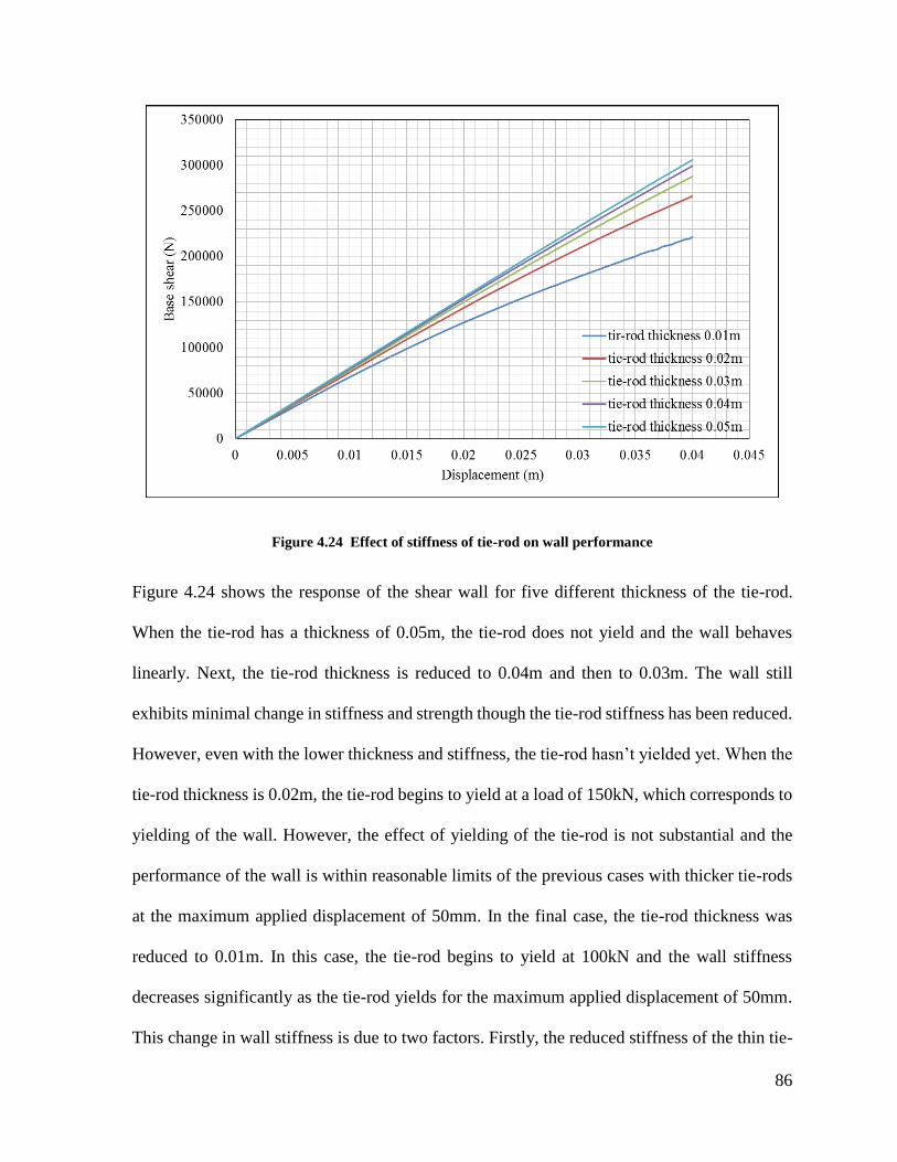
86
Figure 4.24 Effect of stiffness of tie-rod on wall performance
Figure 4.24 shows the response of the shear wall for five different thickness of the tie-rod.
When the tie-rod has a thickness of 0.05m, the tie-rod does not yield and the wall behaves
linearly. Next, the tie-rod thickness is reduced to 0.04m and then to 0.03m. The wall still
exhibits minimal change in stiffness and strength though the tie-rod stiffness has been reduced.
However, even with the lower thickness and stiffness, the tie-rod hasn’t yielded yet. When the
tie-rod thickness is 0.02m, the tie-rod begins to yield at a load of 150kN, which corresponds to
yielding of the wall. However, the effect of yielding of the tie-rod is not substantial and the
performance of the wall is within reasonable limits of the previous cases with thicker tie-rods
at the maximum applied displacement of 50mm. In the final case, the tie-rod thickness was
reduced to 0.01m. In this case, the tie-rod begins to yield at 100kN and the wall stiffness
decreases significantly as the tie-rod yields for the maximum applied displacement of 50mm.
This change in wall stiffness is due to two factors. Firstly, the reduced stiffness of the thin tie-
87
rods contributes directly to lower the stiffness of the wall. Secondly, as the tie-rod begins to
yield, its stiffness decreases significantly, which results in large deformations at the corners of
the opening. This in turn prevents the wall to deform as a single unit, further decreasing the
stiffness of the wall. Therefore, it is preferred to design the tie-rods to behave linearly at loads
lower than the desired strength of the wall. This will ensure that even at the maximum load of
the wall, the system will deform as a single unit. Consider the wall presented in Section 4.6,
which had a maximum load of 100kN. For this wall, a tie-rod of thickness 0.01m would be
sufficient as the tie-rod begins to yield at this load. The study in this section shows that the tie-
rods should preferably be designed to behave linearly for the design load on the wall.
4.12 Conclusions
In this chapter, the use of tie-rods as reinforcement around opening corners in a coupled panel
CLT shear wall has been discussed. A finite element model is developed that can simulate the
behaviour of a coupled panel CLT shear wall with an opening. The finite element model was
then used to highlight the increase in strength and stiffness of the wall when tie-rods are used
as reinforcements around the opening corners.
The modeling approach developed was then used to simulate the behaviour of two different
wall configurations, which highlighted the effect of anchoring on the performance of the shear
wall. The design transfer force for the two wall configurations was also observed to be
significantly affected by the anchoring layout. The Diekmann method was used to determine
the design transfer force and found to provide reasonable estimates for Configuration 1 and
Configuration 2. Therefore the Diekmann model can be used to determine the design transfer
force for reinforcing corners of a simple window-type opening in a CLT shear wall.

88
The effect of tie-rod thickness on the wall behaviour was also studied and it was found that
over designing the tie-rods has minimal impact on the wall performance. Also, yielding of the
tie-rods significantly reduced the wall stiffness and strength. The results from the finite element
analysis indicate that a capacity-based design of the tie-rods to ensure their linear behaviour is
suitable for optimum performance of the wall.
89
Chapter 5: Linear Regression Model for Stiffness of a Wall
In this chapter, the development of a linear regression model to predict the stiffness of a CLT
shear wall with a window-type opening is explained. The previous chapters in this thesis
focused on the forces around corners of an opening and reinforcement requirements. The
objective in this chapter is to develop a regression model that provides insight into the effect
of material property and geometry of the wall on its stiffness. As this probabilistic model
provides a physical quantity as output, it can also be incorporated into the unified reliability
analysis (URA) (Haukaas 2008) framework for performance-based earthquake engineering
(PBEE). An important assumption in this model is that the wall is simply supported at the base.
As the wall-to-floor connection contributes significantly to the force-deformation response of
a wall, the regression model developed here cannot be used to predict the wall behaviour.
5.1 General Form of a Linear Regression Model
A linear regression model is a predictive model, which predicts a response y based on certain
physically measurable variables. The general form a linear regression model is,
kk xxxxy ...332211 (35)
where, y is the response that the regression model predicts, sometimes called as response or
output. xi are the physically measurable variables called as regressors or explanatory variables.
θi are the model parameters, which are also called as regression coefficient. ε represents the
model error, i.e., the difference model prediction and observed response. The model is linear
with respect to the model parameters and not the explanatory variables. This implies that in a
linear regression model the model parameters have unit power, but the explanatory variables
can take the form (x1)0.5 or (x2/x3).
90
Let x denote the k-dimensional vector of explanatory variables. Each trial of the experiment
can be represented by a vector x of the explanatory variables and response y. For n such trials,
the observations of these trials can be collected in an n-by-k dimensional matrix, X and an n-
dimensional vector of y. Similarly, the model parameters can be collected in an n-by-k
dimensional matrix θ. The discrepancy between model prediction and observation can be
represented by a vector ε. The information collected in n-trials can be contained in the
following system of equations,
εθXy (36)
where, ε represents the discrepancy between the observed response y and the value predicted
by the regression model. Eq. (36) forms the basis for determining the characteristics of θ and
ε, which is the primary objective in regression analysis. The inference of the model parameters
θ and the error ε is first carried out using the method of ordinary least squares to obtain point
estimates and then using Bayesian inference.
The method of ordinary least squares provides point estimates of model parameters θ and ε
(Box and Tiao 2001). This does not yield a probabilistic model but provides useful insight and
serves as an input for the Bayesian approach. In this approach, the point estimate of θ is
obtained by minimizing the sum of squared errors. The point estimate of model parameters, θ,
is denoted by θ̂ . The sum of squared errors is given as,
22
2
2
1
2.... n ε (37)
By introducing Eq. (36), the point estimate θ̂ is given as,
22minargmin argˆ Xθyεθ (38)
91
The solution can be obtained by equating the derivative of the objective function with respect
to θ to zero, which is given as,
022
2
XθXyX
θ
XθyTT (39)
Solving Eq. (39) the point estimate θ̂ is given as,
yXXXθTT 1ˆ
(40)
The model error, ε, in the method of ordinary least squares is calculated as the difference
between each observation, y, and the corresponding prediction, kk xθxθxθ ˆ....ˆˆ2211 . It
is assumed that each error is a random variable with zero mean and standard deviation σ, i.e.,
ε~(0, σ2In). The observed error, ε, is given as the difference between the observed response y
and the predicted response X θ̂ . Therefore, based on classical statistics, the estimate of the
standard deviation, σ, is given as,
θXyθXy ˆˆ12
T
kns (41)
where, s is the estimate of σ, often called as the standard error. θXy ˆ is the observed error ε.
k is the number of explanatory variables in the model and n is the number of trials of the
experiment. After determining the point estimates of the model parameters and the standard
errors, a Bayesian approach can be adopted to determine the same in a probabilistic manner.
In the Bayesian approach, the model parameters, θ, and the model error, ε, are treated as
random variables. In a classical regression model, the model error, ε, is normally distributed
with zero mean and standard deviation σ. The objective of Bayesian inference is to determine
the probability distribution of θ as well as σ. Assuming non-informative priors for the
92
distribution of θ and σ, given the observations of y, the posterior distribution of θ is the
multivariate t-distribution, which is given as,
kv
TT
kk
Tk
vsvv
skv
f(
2
1
2
2
ˆˆ1
2
1
2
1
2
1
)θθXXθθ
XX
θ (42)
and the posterior distribution of σ is given by the inverse chi-squared distribution as,
22 ) vvsf( (43)
where, v is the degrees of freedom given as the difference between n and k. θ̂ and s are important
quantities in the posterior probability distributions. This implies that error in estimation of θ̂
and s will affect the Bayesian estimates as well. The explanation in this section provides
necessary insight into the procedure adopted to determine the model parameters and model
error.
5.2 Model Development
The regression model is a predictive model based on statistical analysis of an observed
response. In order to carry out the statistical analysis, repeated trials of an experiment need to
be observed. In this chapter, the experiment is the lateral loading of a simply-supported CLT
shear wall with an opening and the observed response is the stiffness of the wall. The trials of
this experiment is carried out using the finite element model, Model A, whose development
has been explained in Section 2.6.
The regression model takes regressors as input, which in this case are the geometrical and
material parameters of the CLT shear wall, which are summarized in Table 5.1. The
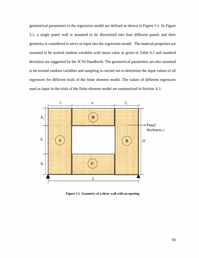
93
geometrical parameters in the regression model are defined as shown in Figure 5.1. In Figure
5.1, a single panel wall is assumed to be discretized into four different panels and their
geometry is considered to serve as input into the regression model. The material properties are
assumed to be normal random variables with mean value as given in Table 4.1 and standard
deviation are suggested by the JCSS Handbook. The geometrical parameters are also assumed
to be normal random variables and sampling is carried out to determine the input values of all
regressors for different trials of the finite element model. The values of different regressors
used as input in the trials of the finite element model are summarized in Section A.1.
Figure 5.1 Geometry of a shear wall with an opening
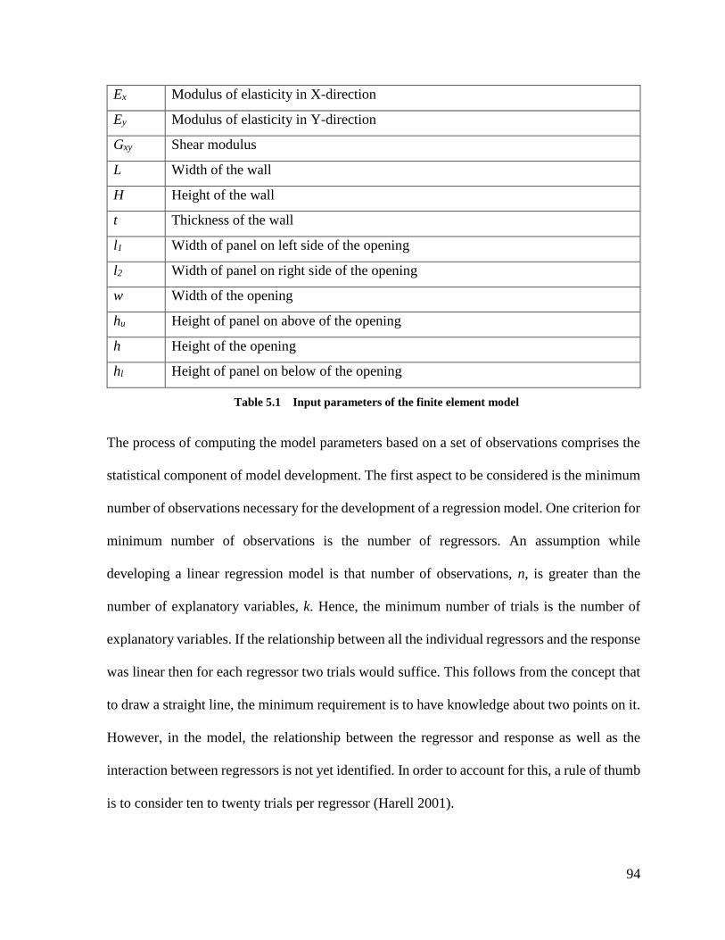
94
Ex Modulus of elasticity in X-direction
Ey Modulus of elasticity in Y-direction
Gxy Shear modulus
L Width of the wall
H Height of the wall
t Thickness of the wall
l1 Width of panel on left side of the opening
l2 Width of panel on right side of the opening
w Width of the opening
hu Height of panel on above of the opening
h Height of the opening
hl Height of panel on below of the opening
Table 5.1 Input parameters of the finite element model
The process of computing the model parameters based on a set of observations comprises the
statistical component of model development. The first aspect to be considered is the minimum
number of observations necessary for the development of a regression model. One criterion for
minimum number of observations is the number of regressors. An assumption while
developing a linear regression model is that number of observations, n, is greater than the
number of explanatory variables, k. Hence, the minimum number of trials is the number of
explanatory variables. If the relationship between all the individual regressors and the response
was linear then for each regressor two trials would suffice. This follows from the concept that
to draw a straight line, the minimum requirement is to have knowledge about two points on it.
However, in the model, the relationship between the regressor and response as well as the
interaction between regressors is not yet identified. In order to account for this, a rule of thumb
is to consider ten to twenty trials per regressor (Harell 2001).
95
The wall as shown in Figure 5.1 is discretized into four panels on sides of the opening. Length
of the wall, L and height of the wall, H, are not independent explanatory variables as they are
related to the length and height of each individual panel. Therefore, there are a total of ten
independent explanatory variables, which implies around 200 trials are necessary for
developing the regression model. An initial regression analysis can be performed with these
parameters as regressors. The response of the model is stiffness of the wall, Kw, which is given
as the lateral load necessary for unit lateral deformation of the wall, i.e., P/∆.
The regression analysis is carried out in Rt, an in-house computer program developed for multi-
model probabilistic analysis. The observations are input into the program to obtain the model
parameters and the standard error, which can be studied to provide insight into effect of various
regressors on the stiffness of the wall. The algorithm employed to determine the model
parameters is explained in Section 5.1. The regression model for stiffness of a CLT shear wall
is given as,
thhhwl
lGEEK
lu
xyyxw
10987625
14321 (44)
where, Kw is the stiffness of the CLT shear wall. The regressors in the model are explained in
Table 5.1. The distribution of the model parameters obtained from the regression analysis is
shown in Table 5.2. The standard deviation of the model error is normally distributed with
mean 1.25x1006 and standard deviation 6.45x1004.
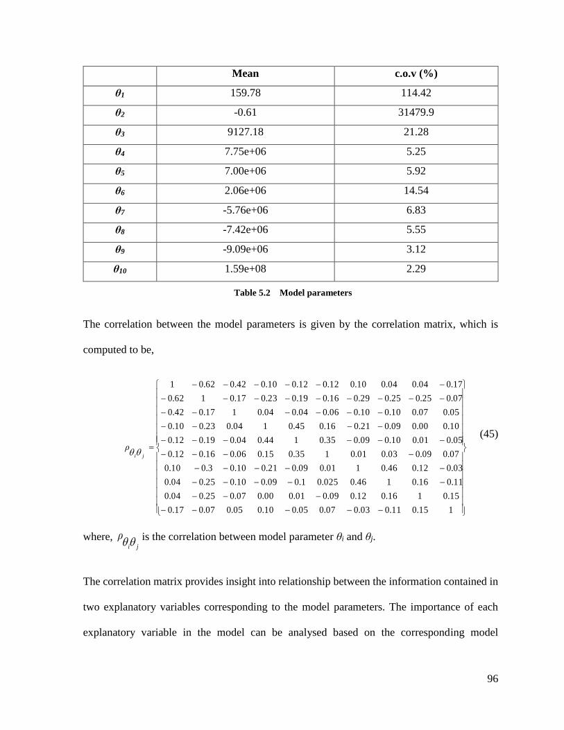
96
Mean c.o.v (%)
θ1 159.78 114.42
θ2 -0.61 31479.9
θ3 9127.18 21.28
θ4 7.75e+06 5.25
θ5 7.00e+06 5.92
θ6 2.06e+06 14.54
θ7 -5.76e+06 6.83
θ8 -7.42e+06 5.55
θ9 -9.09e+06 3.12
θ10 1.59e+08 2.29
Table 5.2 Model parameters
The correlation between the model parameters is given by the correlation matrix, which is
computed to be,
115.011.003.007.005.010.005.007.017.0
15.0116.012.009.001.000.007.025.004.0
11.016.0146.0025.01.009.010.025.004.0
03.012.046.0101.009.021.010.03.010.0
07.009.003.001.0135.015.006.016.012.0
05.001.010.009.035.0144.004.019.012.0
10.000.009.021.016.045.0104.023.010.0
05.007.010.010.006.004.004.0117.042.0
07.025.025.029.016.019.023.017.0162.0
17.004.004.010.012.012.010.042.062.01
ji
ρ
(45)
where, ji
ρ is the correlation between model parameter θi and θj.
The correlation matrix provides insight into relationship between the information contained in
two explanatory variables corresponding to the model parameters. The importance of each
explanatory variable in the model can be analysed based on the corresponding model
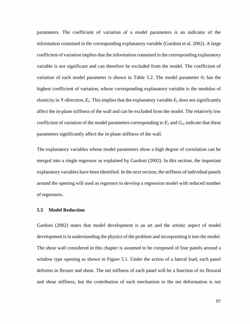
97
parameters. The coefficient of variation of a model parameters is an indicator of the
information contained in the corresponding explanatory variable (Gardoni et al. 2002). A large
coefficient of variation implies that the information contained in the corresponding explanatory
variable is not significant and can therefore be excluded from the model. The coefficient of
variation of each model parameter is shown in Table 5.2. The model parameter θ2 has the
highest coefficient of variation, whose corresponding explanatory variable is the modulus of
elasticity in Y-direction, Ey. This implies that the explanatory variable Ey does not significantly
affect the in-plane stiffness of the wall and can be excluded from the model. The relatively low
coefficient of variation of the model parameters corresponding to Ex and Gxy indicate that these
parameters significantly affect the in-plane stiffness of the wall.
The explanatory variables whose model parameters show a high degree of correlation can be
merged into a single regressor as explained by Gardoni (2002). In this section, the important
explanatory variables have been identified. In the next section, the stiffness of individual panels
around the opening will used as regressor to develop a regression model with reduced number
of regressors.
5.3 Model Reduction
Gardoni (2002) states that model development is an art and the artistic aspect of model
development is in understanding the physics of the problem and incorporating it into the model.
The shear wall considered in this chapter is assumed to be composed of four panels around a
window type opening as shown in Figure 5.1. Under the action of a lateral load, each panel
deforms in flexure and shear. The net stiffness of each panel will be a function of its flexural
and shear stiffness, but the contribution of each mechanism to the net deformation is not
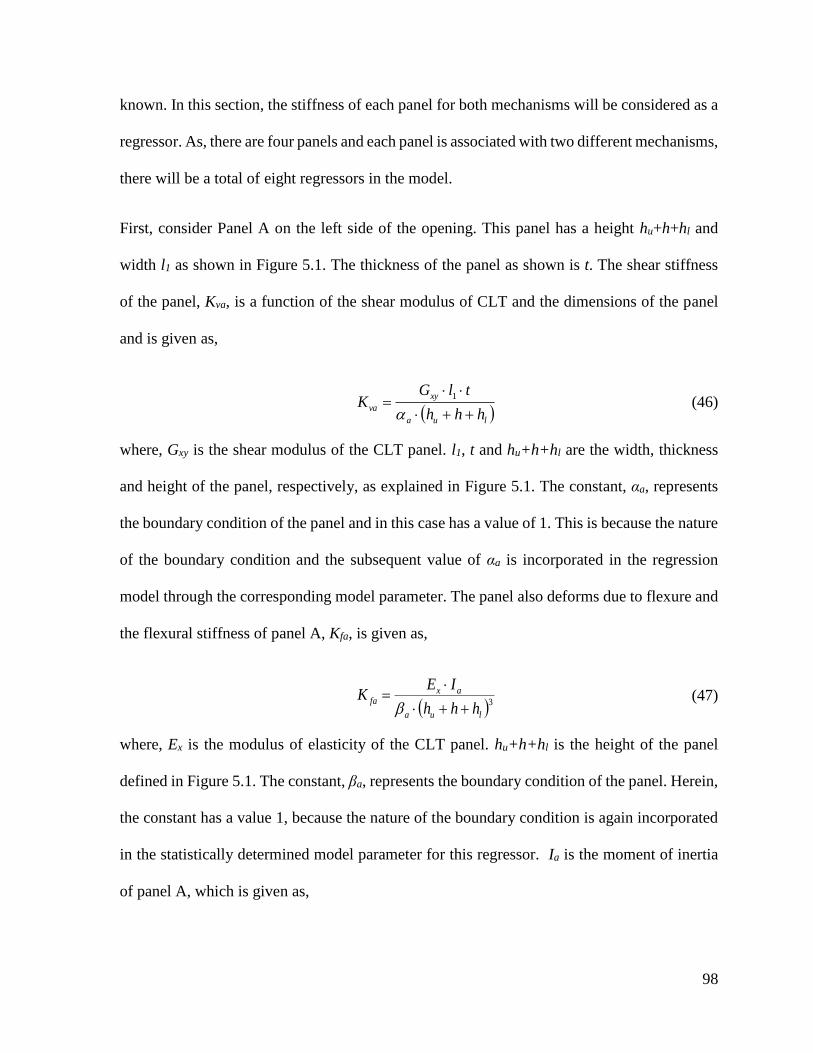
98
known. In this section, the stiffness of each panel for both mechanisms will be considered as a
regressor. As, there are four panels and each panel is associated with two different mechanisms,
there will be a total of eight regressors in the model.
First, consider Panel A on the left side of the opening. This panel has a height hu+h+hl and
width l1 as shown in Figure 5.1. The thickness of the panel as shown is t. The shear stiffness
of the panel, Kva, is a function of the shear modulus of CLT and the dimensions of the panel
and is given as,
lua
xy
vahhh
tlGK
1 (46)
where, Gxy is the shear modulus of the CLT panel. l1, t and hu+h+hl are the width, thickness
and height of the panel, respectively, as explained in Figure 5.1. The constant, αa, represents
the boundary condition of the panel and in this case has a value of 1. This is because the nature
of the boundary condition and the subsequent value of αa is incorporated in the regression
model through the corresponding model parameter. The panel also deforms due to flexure and
the flexural stiffness of panel A, Kfa, is given as,
3lua
axfa
hhh
IEK
(47)
where, Ex is the modulus of elasticity of the CLT panel. hu+h+hl is the height of the panel
defined in Figure 5.1. The constant, βa, represents the boundary condition of the panel. Herein,
the constant has a value 1, because the nature of the boundary condition is again incorporated
in the statistically determined model parameter for this regressor. Ia is the moment of inertia
of panel A, which is given as,

99
12
3
1ltI a
(48)
where, l1 and t are the width and thickness of the panel respectively, as shown in Figure 5.1.
Similarly, the shear and flexural stiffness of panel B, C and D can be established. Panel B has
a shear stiffness, Kvb, which is given as,
ub
xy
vbh
twGK
(49)
where, Gxy is the shear modulus of the CLT panel. w, t and hu are the width, thickness and
height of panel B respectively as defined in Figure 5.1. The constant, αb, represents the
boundary condition of the panel and in this case has a value of 1.
The flexural stiffness of panel B, Kfb, is given as,
3ub
bx
fbh
IEK
(50)
where, Ex is the modulus of elasticity of the CLT panel and hu is the height of the panel as
defined in Figure 5.1. The constant, βb, representing the boundary condition of the panel, has
a value of 1. Ib is the moment of inertia of panel A, which is given as,
12
3wtI b
(51)
where, w and t are the width and thickness of the panel respectively, as shown in Figure 5.1.
Next, consider the deformation of panel C. The panel has a shear stiffness, Kvc, which is given
as,

100
lc
xy
vch
twGK
(52)
where, Gxy is the shear modulus of the CLT panel. w, t and hl are the dimensions of panel B
defined in Figure 5.1. The constant, αc, representing the boundary condition of the panel has a
value of 1.
The flexural stiffness of panel B, Kfc, is given as,
3
lc
cx
fch
IEK
(53)
where, Ex is the modulus of elasticity of the CLT panel and hl is the height of the panel as
defined in Figure 5.1. The constant, βc, representing the boundary condition of the panel, has
a value of 1. Ic is the moment of inertia of panel A, which is given as,
12
3wtI b
(54)
where, w and t are the width and thickness of the panel respectively, as shown in Figure 5.1.
Next, consider the deformation of the full-height panel to the right-side of the opening, which
is denoted as panel D in Figure 5.1. The panel has a shear stiffness, Kvd, which is given as,
lud
xy
vdhhh
tlGK
2 (55)
where, Gxy is the shear modulus of the CLT panel. l2, t and hl+h+hl are the dimensions of panel
B as defined in Figure 5.1. The constant, αd, representing the boundary condition of the panel
has a value of 1. The flexural stiffness of panel D, Kfd, is given as,
3
lud
dx
fdhhh
IEK
(56)

101
where, Ex is the modulus of elasticity of the CLT panel and hl+h+hl is the height of the panel
as defined in Figure 5.1. The constant, βd, representing the boundary condition of the panel,
has a value of 1. Id is the moment of inertia of panel A, which is given as,
12
3
2ltI d
(57)
where, l2 and t are the width and thickness of the panel respectively, as shown in Figure 5.1.
This completes the definition of the regressors to be included in the regression model for
stiffness of the wall. Eq. (46) to Eq. (57) can be used to determine the regressors in the model
for input into Rt to carry out a model inference analysis.
The regression model for stiffness of a CLT shear wall with a window type opening is given
as,
vdfdvcfcvbfbvafaw KKKKKKKKK 87654321 (58)
where, Kw is the stiffness of the CLT shear wall with a window-type opening. The regressors
in the model are the flexural and shear stiffness of each panel shown in Figure 5.1. The model
parameters obtained from the model inference analysis in Rt is shown in Table 5.3. The model
error has zero mean and a standard deviation σ, which is a random variable. The standard
deviation of the model error is normally distributed with mean 1.52x1006 and standard
deviation 7.86x1004. The model parameter of a regressor in the model includes the factor for
contribution of the mechanism to the net deformation of the wall as well as the factor for the
boundary condition of each panel. A look at the coefficient of variation of the model parameters
in Table 5.3 shows that each model parameter is important to the model and has significant
information.
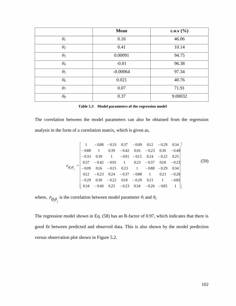
102
Mean c.o.v (%)
θ1 0.16 46.06
θ2 0.41 10.14
θ3 0.00091 94.75
θ4 -0.01 96.38
θ5 -0.00064 97.34
θ6 0.021 40.76
θ7 0.07 71.91
θ8 0.37 9.00032
Table 5.3 Model parameters of the regression model
The correlation between the model parameters can also be obtained from the regression
analysis in the form of a correlation matrix, which is given as,
1850260340230250400340
8501210290180220300290
2602101880370240230120
3402908801230150160090
2301803702301910420370
2502202401509101390330
4003002301604203901880
3402901200903703308801
.......
.......
.......
.......
.......
.......
.......
.......
ρji
(59)
where, ji
ρ is the correlation between model parameter θi and θj.
The regression model shown in Eq. (58) has an R-factor of 0.97, which indicates that there is
good fit between predicted and observed data. This is also shown by the model prediction
versus observation plot shown in Figure 5.2.
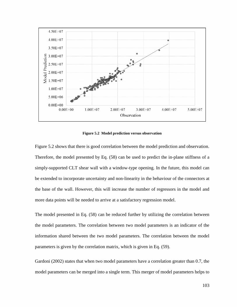
103
Figure 5.2 Model prediction versus observation
Figure 5.2 shows that there is good correlation between the model prediction and observation.
Therefore, the model presented by Eq. (58) can be used to predict the in-plane stiffness of a
simply-supported CLT shear wall with a window-type opening. In the future, this model can
be extended to incorporate uncertainty and non-linearity in the behaviour of the connectors at
the base of the wall. However, this will increase the number of regressors in the model and
more data points will be needed to arrive at a satisfactory regression model.
The model presented in Eq. (58) can be reduced further by utilizing the correlation between
the model parameters. The correlation between two model parameters is an indicator of the
information shared between the two model parameters. The correlation between the model
parameters is given by the correlation matrix, which is given in Eq. (59).
Gardoni (2002) states that when two model parameters have a correlation greater than 0.7, the
model parameters can be merged into a single term. This merger of model parameters helps to
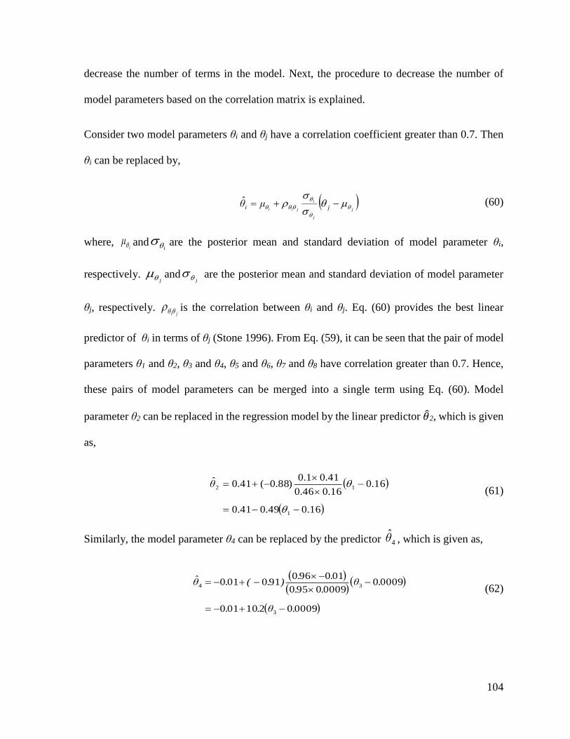
104
decrease the number of terms in the model. Next, the procedure to decrease the number of
model parameters based on the correlation matrix is explained.
Consider two model parameters θi and θj have a correlation coefficient greater than 0.7. Then
θi can be replaced by,
j
j
i
jii ji μθ
ˆ (60)
where, i
μ andi
are the posterior mean and standard deviation of model parameter θi,
respectively. j
andj are the posterior mean and standard deviation of model parameter
θj, respectively. ji
is the correlation between θi and θj. Eq. (60) provides the best linear
predictor of θi in terms of θj (Stone 1996). From Eq. (59), it can be seen that the pair of model
parameters θ1 and θ2, θ3 and θ4, θ5 and θ6, θ7 and θ8 have correlation greater than 0.7. Hence,
these pairs of model parameters can be merged into a single term using Eq. (60). Model
parameter θ2 can be replaced in the regression model by the linear predictor 𝜃2, which is given
as,
16.049.041.0
16.016.046.0
41.01.0)88.0(41.0ˆ
1
12
θ (61)
Similarly, the model parameter θ4 can be replaced by the predictor 4θ̂ , which is given as,
00090210010
0009000090950
010960910010ˆ
3
34
.θ..
.θ..
..).(.θ
(62)
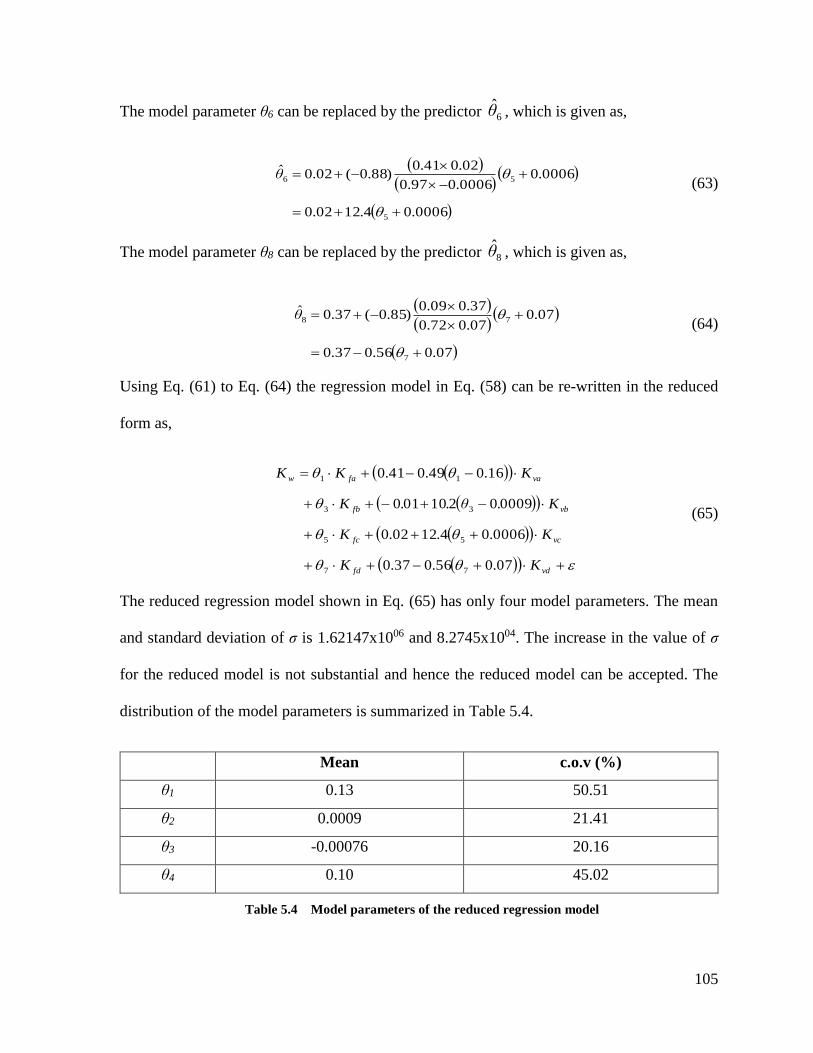
105
The model parameter θ6 can be replaced by the predictor 6θ̂ , which is given as,
0006.04.1202.0
0006.00006.097.0
02.041.0)88.0(02.0ˆ
5
56
θ (63)
The model parameter θ8 can be replaced by the predictor 8θ̂ , which is given as,
07.056.037.0
07.007.072.0
37.009.0)85.0(37.0ˆ
7
78
θ (64)
Using Eq. (61) to Eq. (64) the regression model in Eq. (58) can be re-written in the reduced
form as,
vdfd
vcfc
vbfb
vafaw
KK
KK
K.θ..K
KKK
07.056.037.0
0006.04.1202.0
00090210010
16.049.041.0
77
55
33
11
(65)
The reduced regression model shown in Eq. (65) has only four model parameters. The mean
and standard deviation of σ is 1.62147x1006 and 8.2745x1004. The increase in the value of σ
for the reduced model is not substantial and hence the reduced model can be accepted. The
distribution of the model parameters is summarized in Table 5.4.
Mean c.o.v (%)
θ1 0.13 50.51
θ2 0.0009 21.41
θ3 -0.00076 20.16
θ4 0.10 45.02
Table 5.4 Model parameters of the reduced regression model

106
The correlation between the model parameters is given as,
1006.007.076.0
006.0132.033.0
07.032.0127.0
76.033.027.01
ji
ρ
(66)
Therefore, Eq. (58) and Eq. (65) can be used to determine the in-plane stiffness of a simply-
supported CLT shear wall with a window-type opening. In the future, Eq. (65) can be improved
by obtaining more data, preferably experimental data and incorporating the behaviour of
connectors as regressors in the model. This will significantly increase the confidence in the
predictions from the regression model.

107
Chapter 6: Conclusion and Future Work
This chapter presents a broader perspective of the results from this thesis. The objective of this
chapter is to demonstrate the manner in which this thesis addresses present research gap and
provides a foundation for future work in this field.
6.1 Conclusion
The introduction chapter highlighted the lack of research carried out in applying the FTAO
design paradigm to CLT shear walls. The literature review also highlighted the need for better
models to determine the transfer force at the corners of an opening. The analytical models in
literature for FTAO were developed for designing reinforcements around the corners of
openings in timber frame shear walls.
This thesis addresses the development of transfer force around opening corners in CLT shear
walls. The focus of this thesis is to study the development of transfer force in CLT as opposed
to the more widely researched field of timber-frame shear walls. The objective is to understand
the type of transfer force that develops in CLT for different construction practices.
The methodology adopted to analyse CLT shear walls is development of finite element models
in ANSYS. Numerical models developed address the difference in stress redistribution
observed for different construction practices. The library of numerical models presented help
in simulating the behaviour of CLT shear walls with different types of openings.
The models are also amenable for use in different seismic design frameworks such as PBEE,
DDBD and force-based design. The models can be used for capacity-based design of shear
walls and to design appropriate connection layouts.
108
6.2 Future Work
The scope for the future in this project lies in two directions. Firstly, there has been no
experimental work conducted in this project. It will be an asset to conduct an experimental
investigation to corroborate the predictions from the numerical models. Also, analysis of the
cut-out opening type construction practice indicates that shear in wood panels around opening
corners could be a potential source of failure, which needs to be experimentally verified.
Tie-rods have been recommended for reinforcing the corners of an opening in a coupled-panel
CLT wall. The Diekmann method can be used to design the tie-rods for a wall set-up to
experimentally verify the importance of reinforcing opening corners.
The second aspect to be considered in the future would be improvement of the models
developed in this thesis. In the future, the models can be improved to capture visual damage in
connectors, CLT panels and the glued surface. Connection models can be improved to
incorporate cyclic behaviour for use in dynamic analysis. The finite element models can be
used in a unified reliability analysis framework to optimize the cross-section, length and
location of the tie-rods as well as design of the wall anchors. The linear regression model
presented in this thesis can be refined in future to incorporate the non-linearity and uncertainty
in behaviour of anchors and other wall connectors
George E. P. Box in his book Empirical Model-Building and Response Surfaces wrote,
“Essentially, all models are wrong, but some are useful.” The scope for the future is to make
use of the models in this thesis, to develop a PBEE framework for design of CLT shear walls
based on force transfer around openings.
109
References
ANSYS. (2012). ANSYS Mechanical APDL Command Reference.
ANSYS. (2012). ANSYS Mechanical APDL Element Reference.
Ang, A. H. S., and Tang, Wi. S. (2006). Probability Concepts in Engineering: Emphasis on
Applications to Civil and Environmental Engineering.
Ashtari, S. (2012). “In-plane Stiffness of Cross-laminated Timber Floors.” University of
British Columbia, (M.A.Sc. Thesis).
Blasetti, A., Hoffman, R., and Dinehart, D. W. (2006). “A Simplified Wood Sheathing
Connection Model using ANSYS.” 2006 ANSYS Conference, Pittsburgh, PA.
Blasetti, A., Hoffman, R., and Dinehart, D. W. (2008). “Simplified hysteretic finite-element
model for wood and viscoelastic polymer connections for the dynamic analysis of shear
walls.” Journal of structural engineering, 134(1), 77–86.
Bogensperger, T., Moosbrugger, T., and Silly, G. (2010). “Verification of CLT-plates under
loads in plane.” World Conference on Timber Engineering, 20–24.
Box, G. E., and Tiao, G. C. (2001). Bayesian inference in statistical analysis. John Wiley &
Sons.
Breyer, D. E., and Ank, J. A. (1980). Design of wood structures. Mc-Graw Hill Book
Company.
Breyer, D. E., Fridley, K. J., Cobeen, K. E., and Pollock, D. G. (2007). “Shearwalls.” Design
of Wood Structures.
Ceccotti, A., and Follesa, M. (2006). “Seismic behaviour of multi-storey X-lam buildings.”
COST E29 International Workshop on Earthquake Engineering on Timber Structures.
Ceccotti, A., Follesa, M., and Karacabeyli, E. (2000). “3D seismic analysis of multi-storey
wood frame construction.” Atti del World Conference on Timber Engineering.
Ceccotti, A., Follesa, M., Lauriola, M. P., and Sandhaas, C. (2006). “Sofie Project–Test Results
on the Lateral Resistance of Cross-Laminated Wooden Panels.” Proceedings of the First
European Conference on Earthquake Engineering and Seismicity, 3.
Ceccotti, A., and Karacabeyli, E. (2002). “Validation of Seismic Design Parameters for Wood-
frame Shearwall Systems.” Canadian Journal of Civil Engineering, 29(3), 484–498.
“CST Innovations.” (2011). <http://www.cstinnovations.ca/sustainability.php>.
110
Diekmann, E. F. (1995). “Diaphragms and Shearwalls.” Wood Engineering and Construction
Handbook, K. F. Faherty and T. G. Williamson, eds., 8.1–8.78.
Dolan, J. D. (1989). “The Dynamic Response of Timber Shear Walls.” University of British
Columbia, Ph.D. Thes(October).
Dolan, J. D., and Heine, C. P. (1997). Monotonic Tests of Wood-frame Shear Walls with
Various Openings and Base Restraint Configurations. Virginia Polytechnic Institute and
State University, Blacksburg.
Dujic, B., Klobcar, S., and Zarnic, R. (2008). “Shear Capacity of Cross-Laminated Wooden
Walls.” Proceedings of the 40th CIB-W18 Meeting., Vol. 40.
“Earthquakes Canada.” (2014). Natural Resources Canada,
<http://www.earthquakescanada.nrcan.gc.ca/recent/maps-cartes/index-
eng.php?tpl_region=west&maptype=1y>.
Filiatrault, A., and Folz, B. (2002). “Performance-based Seismic Design of Wood Framed
Buildings.” Journal of Structural Engineering, 128(1), 39–47.
Filiatrault, A., Isoda, H., and Folz, B. (2003). “Hysteretic Damping of Wood Framed
Buildings.” Engineering Structures, 25(4), 461–471.
Folz, B., and Filiatrault, A. (2004). “Seismic Analysis of Woodframe Structures. I: Model
Formulation.” Journal of Structural Engineering, 130(9), 1353–1360.
Gagnon, S., and Popovski, M. (2011). “Structural design of cross-laminated timber elements.”
CLT Handbook.
Gardoni, P., Der Kiureghian, A., and Mosalam, K. M. (2002). “Probabilistic capacity models
and fragility estimates for reinforced concrete columns based on experimental
observations.” Journal of Engineering Mechanics, 128(October), 1024–1038.
Gavric, I. (2012). “Seismic Behaviour of Cross-Laminated Timber Buildings.” University of
Trieste, (Ph.D. Thesis).
Gavric, I., Rinaldin, G., Amadio, C., Fragiacomo, M., and Ceccotti, A. (2012). “Experimental-
numerical analyses of the seismic behaviour of cross-laminated wall systems.” 15th
World Conference on Earthquake Engineering.
Gsell, D., Feltrin, G., Schubert, S., Steiger, R., and Motavalli, M. (2007). “Cross-Laminated
Timber Plates : Evaluation and Verification of Homogenized Elastic Properties.” Journal
of Structural Engineering, 133(January), 132–138.
Harell, F. E. (2001). Regression modeling strategies: with applications to linear models,
logistic regression, and survival analysis. Springer.
111
Haukaas, T. (2008). “Unified reliability and design optimization for earthquake engineering.”
Probabilistic Engineering Mechanics, 23(4), 471–481.
IBC, I. (2006). “International building code.” International Code Council, Inc.(formerly
BOCA, ICBO and SBCCI).
Joebstl, R., Bogensperger, T., and Schickhofer, G. (2008). “In-plane Shear Strength of Cross
Laminated Timber.” Proceedings of CIB-W18 Timber Engineering, (August).
Kirkegaard, P. H., Sørensen, J. D., Čizmar, D., and Rajčić, V. (2011). “System Reliability of
Timber Structures with Ductile Behaviour.” Engineering Structures, Elsevier Ltd, 33(11),
3093–3098.
Kuilen, J. W. G. V. De, Ceccotti, A., Xia, Z., and He, M. (2011). “Very Tall Wooden Buildings
with Cross Laminated Timber.” Procedia Engineering, 14, 1621–1628.
Li, M., Lam, F., Yeh, B., Skaggs, T., Rammer, D., and Wacker, J. (2012). “Modeling Force
Transfer around Openings in Wood-Frame Shear Walls.” Journal of Structural
Engineering, 138(12), 1419–1426.
Lindt, J. W. van de, Rosowsky, D. V, Pang, W., and Pei, S. (2013). “Performance-Based
Seismic Design of Mid-Rise Woodframe Buildings.” Journal of Structural Engineering,
139(8), 1294–1302.
Line, P., and Douglas, B. K. (1996). “Perforated Shearwall Design Method.” International
Wood Engineering Conference, 28–31.
Mahsuli, M., and Haukaas, T. (2013a). “Computer program for multimodel reliability and
optimization analysis.” Journal of Computing in Civil Engineering, 27(1), 87–98.
Mahsuli, M., and Haukaas, T. (2013b). “Seismic risk analysis with reliability methods, part I:
Models.” Structural Safety, 42, 54–62.
Martin, Z. (2005). “Design of Wood Structural Panel Shear Walls with Openings: A
Comparison of Methods.” Wood Design Focus, 15(1), 18–20.
Moosbrugger, T., Guggenberger, W., and Bogensperger, T. (2006). “Cross-Laminated Timber
Wall Segments under Homogeneous Shear — with and without Openings.” WCTE 2006-
9th International Conference on Timber Engineering.
Noory, M., Smith, I., and Asiz, A. (2010). “Tests and Numerical Models for Shear-walls with
Various Layers.” 11th World Conference on Timber Engineering, 20–24.
Pang, W., and Rosowsky, D. (2007). “Direct Displacement Procedure for Performance-based
Seismic Design of Multistory Woodframe Structures.” NEESWood Report NW, 2(June).
112
Pei, S., Popovski, M., and Lindt, J. W. Van De. (2012). “Seismic Design of a Multi-story Cross
Laminated Timber Building based on Component Level Testing.” World Conference on
Timber Engineering, (July), 244–252.
Popovski, M., Karacabeyli, E., and Ceccotti, A. (2011). “Seismic Performance of Cross-
laminated Timber Buildings.” CLT Handbook, FP Innovation.
Popovski, M., Schneider, J., and Schweinsteiger, M. (2010). “Lateral Load Resistance of
Cross-laminated Wood Panels.” World Conference on Timber Engineering, 20–24.
Robertson, A. (2009). “Design for Force Transfer Around Openings: A Comparison of
Methodologies.” Robertson and Associates.
Rosowsky, D. (2002). “Reliability-based Seismic Design of Wood Shear Walls.” Journal of
Structural Engineering, (November), 1439–1453.
Salenikovich, A. J., and Dolan, J. D. (2003). “The Racking Performance of Shear Walls with
Various Aspect Ratios: Part 1- Monotonic Tests of Fully Anchored Walls.” Forest
Products Journal, 53(10), 65–73.
Schneider, J., Stiemer, S., Tesfamariam, S., Karacabeyli, E., and Popovski, M. (2012).
“Damage Assessment of Cross Laminated Timber Connections Subjected to Simulated
Earthquake Loads.” World Conference on Timber Engineering, 15(July), 398–406.
Skaggs, T., Yeh, B., Lam, F., Rammer, D., and Wacker, J. (2010). “Full-Scale Shear Wall
Tests for Force Transfer Around Openings.” International Council for Research and
Innovation in Building and Construction-Working Commission W18--Timber Structures,
22–26.
Stone, C. J. (1996). A course in probability and statistics. Duxbury Press.
Structurlam. (n.d.). Cross-Laminated Timber Design Guide.
Yawalata, D., and Lam, F. (2011). Development of Technology for Cross Laminated Timber
Building Systems. Vancouver.
Yeh, B., Skaggs, T., Lam, F., Li, M., Rammer, D., and Wacker, J. (2011). Evaluation of Force
Transfer Around Openings – Experimental and Analytical Studies.
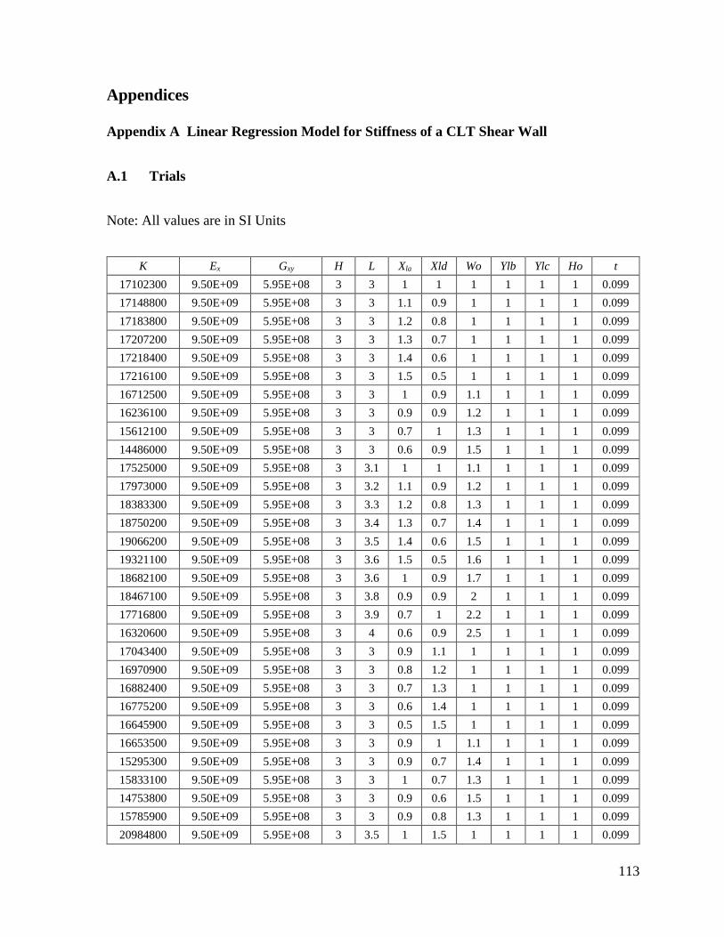
113
Appendices
Appendix A Linear Regression Model for Stiffness of a CLT Shear Wall
A.1 Trials
Note: All values are in SI Units
K Ex Gxy H L Xla Xld Wo Ylb Ylc Ho t
17102300 9.50E+09 5.95E+08 3 3 1 1 1 1 1 1 0.099
17148800 9.50E+09 5.95E+08 3 3 1.1 0.9 1 1 1 1 0.099
17183800 9.50E+09 5.95E+08 3 3 1.2 0.8 1 1 1 1 0.099
17207200 9.50E+09 5.95E+08 3 3 1.3 0.7 1 1 1 1 0.099
17218400 9.50E+09 5.95E+08 3 3 1.4 0.6 1 1 1 1 0.099
17216100 9.50E+09 5.95E+08 3 3 1.5 0.5 1 1 1 1 0.099
16712500 9.50E+09 5.95E+08 3 3 1 0.9 1.1 1 1 1 0.099
16236100 9.50E+09 5.95E+08 3 3 0.9 0.9 1.2 1 1 1 0.099
15612100 9.50E+09 5.95E+08 3 3 0.7 1 1.3 1 1 1 0.099
14486000 9.50E+09 5.95E+08 3 3 0.6 0.9 1.5 1 1 1 0.099
17525000 9.50E+09 5.95E+08 3 3.1 1 1 1.1 1 1 1 0.099
17973000 9.50E+09 5.95E+08 3 3.2 1.1 0.9 1.2 1 1 1 0.099
18383300 9.50E+09 5.95E+08 3 3.3 1.2 0.8 1.3 1 1 1 0.099
18750200 9.50E+09 5.95E+08 3 3.4 1.3 0.7 1.4 1 1 1 0.099
19066200 9.50E+09 5.95E+08 3 3.5 1.4 0.6 1.5 1 1 1 0.099
19321100 9.50E+09 5.95E+08 3 3.6 1.5 0.5 1.6 1 1 1 0.099
18682100 9.50E+09 5.95E+08 3 3.6 1 0.9 1.7 1 1 1 0.099
18467100 9.50E+09 5.95E+08 3 3.8 0.9 0.9 2 1 1 1 0.099
17716800 9.50E+09 5.95E+08 3 3.9 0.7 1 2.2 1 1 1 0.099
16320600 9.50E+09 5.95E+08 3 4 0.6 0.9 2.5 1 1 1 0.099
17043400 9.50E+09 5.95E+08 3 3 0.9 1.1 1 1 1 1 0.099
16970900 9.50E+09 5.95E+08 3 3 0.8 1.2 1 1 1 1 0.099
16882400 9.50E+09 5.95E+08 3 3 0.7 1.3 1 1 1 1 0.099
16775200 9.50E+09 5.95E+08 3 3 0.6 1.4 1 1 1 1 0.099
16645900 9.50E+09 5.95E+08 3 3 0.5 1.5 1 1 1 1 0.099
16653500 9.50E+09 5.95E+08 3 3 0.9 1 1.1 1 1 1 0.099
15295300 9.50E+09 5.95E+08 3 3 0.9 0.7 1.4 1 1 1 0.099
15833100 9.50E+09 5.95E+08 3 3 1 0.7 1.3 1 1 1 0.099
14753800 9.50E+09 5.95E+08 3 3 0.9 0.6 1.5 1 1 1 0.099
15785900 9.50E+09 5.95E+08 3 3 0.9 0.8 1.3 1 1 1 0.099
20984800 9.50E+09 5.95E+08 3 3.5 1 1.5 1 1 1 1 0.099
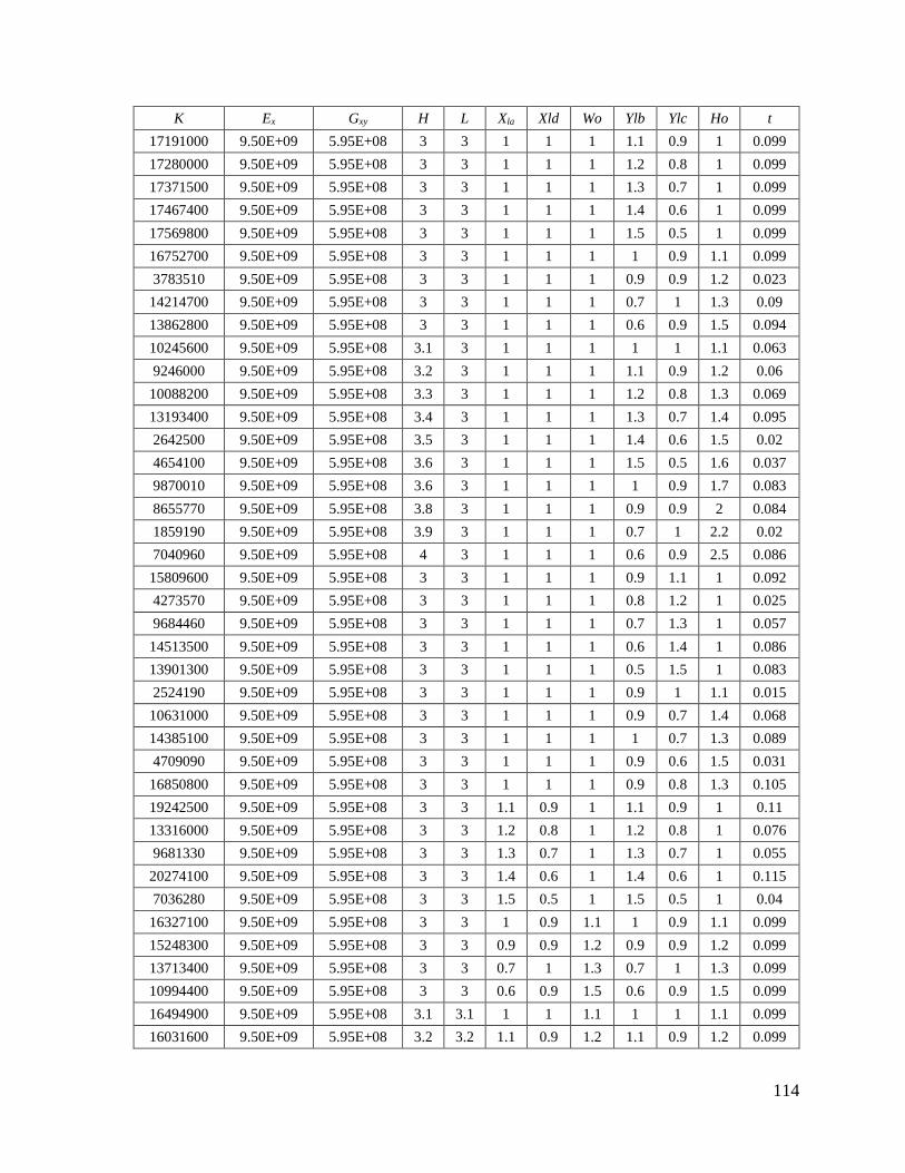
114
K Ex Gxy H L Xla Xld Wo Ylb Ylc Ho t
17191000 9.50E+09 5.95E+08 3 3 1 1 1 1.1 0.9 1 0.099
17280000 9.50E+09 5.95E+08 3 3 1 1 1 1.2 0.8 1 0.099
17371500 9.50E+09 5.95E+08 3 3 1 1 1 1.3 0.7 1 0.099
17467400 9.50E+09 5.95E+08 3 3 1 1 1 1.4 0.6 1 0.099
17569800 9.50E+09 5.95E+08 3 3 1 1 1 1.5 0.5 1 0.099
16752700 9.50E+09 5.95E+08 3 3 1 1 1 1 0.9 1.1 0.099
3783510 9.50E+09 5.95E+08 3 3 1 1 1 0.9 0.9 1.2 0.023
14214700 9.50E+09 5.95E+08 3 3 1 1 1 0.7 1 1.3 0.09
13862800 9.50E+09 5.95E+08 3 3 1 1 1 0.6 0.9 1.5 0.094
10245600 9.50E+09 5.95E+08 3.1 3 1 1 1 1 1 1.1 0.063
9246000 9.50E+09 5.95E+08 3.2 3 1 1 1 1.1 0.9 1.2 0.06
10088200 9.50E+09 5.95E+08 3.3 3 1 1 1 1.2 0.8 1.3 0.069
13193400 9.50E+09 5.95E+08 3.4 3 1 1 1 1.3 0.7 1.4 0.095
2642500 9.50E+09 5.95E+08 3.5 3 1 1 1 1.4 0.6 1.5 0.02
4654100 9.50E+09 5.95E+08 3.6 3 1 1 1 1.5 0.5 1.6 0.037
9870010 9.50E+09 5.95E+08 3.6 3 1 1 1 1 0.9 1.7 0.083
8655770 9.50E+09 5.95E+08 3.8 3 1 1 1 0.9 0.9 2 0.084
1859190 9.50E+09 5.95E+08 3.9 3 1 1 1 0.7 1 2.2 0.02
7040960 9.50E+09 5.95E+08 4 3 1 1 1 0.6 0.9 2.5 0.086
15809600 9.50E+09 5.95E+08 3 3 1 1 1 0.9 1.1 1 0.092
4273570 9.50E+09 5.95E+08 3 3 1 1 1 0.8 1.2 1 0.025
9684460 9.50E+09 5.95E+08 3 3 1 1 1 0.7 1.3 1 0.057
14513500 9.50E+09 5.95E+08 3 3 1 1 1 0.6 1.4 1 0.086
13901300 9.50E+09 5.95E+08 3 3 1 1 1 0.5 1.5 1 0.083
2524190 9.50E+09 5.95E+08 3 3 1 1 1 0.9 1 1.1 0.015
10631000 9.50E+09 5.95E+08 3 3 1 1 1 0.9 0.7 1.4 0.068
14385100 9.50E+09 5.95E+08 3 3 1 1 1 1 0.7 1.3 0.089
4709090 9.50E+09 5.95E+08 3 3 1 1 1 0.9 0.6 1.5 0.031
16850800 9.50E+09 5.95E+08 3 3 1 1 1 0.9 0.8 1.3 0.105
19242500 9.50E+09 5.95E+08 3 3 1.1 0.9 1 1.1 0.9 1 0.11
13316000 9.50E+09 5.95E+08 3 3 1.2 0.8 1 1.2 0.8 1 0.076
9681330 9.50E+09 5.95E+08 3 3 1.3 0.7 1 1.3 0.7 1 0.055
20274100 9.50E+09 5.95E+08 3 3 1.4 0.6 1 1.4 0.6 1 0.115
7036280 9.50E+09 5.95E+08 3 3 1.5 0.5 1 1.5 0.5 1 0.04
16327100 9.50E+09 5.95E+08 3 3 1 0.9 1.1 1 0.9 1.1 0.099
15248300 9.50E+09 5.95E+08 3 3 0.9 0.9 1.2 0.9 0.9 1.2 0.099
13713400 9.50E+09 5.95E+08 3 3 0.7 1 1.3 0.7 1 1.3 0.099
10994400 9.50E+09 5.95E+08 3 3 0.6 0.9 1.5 0.6 0.9 1.5 0.099
16494900 9.50E+09 5.95E+08 3.1 3.1 1 1 1.1 1 1 1.1 0.099
16031600 9.50E+09 5.95E+08 3.2 3.2 1.1 0.9 1.2 1.1 0.9 1.2 0.099
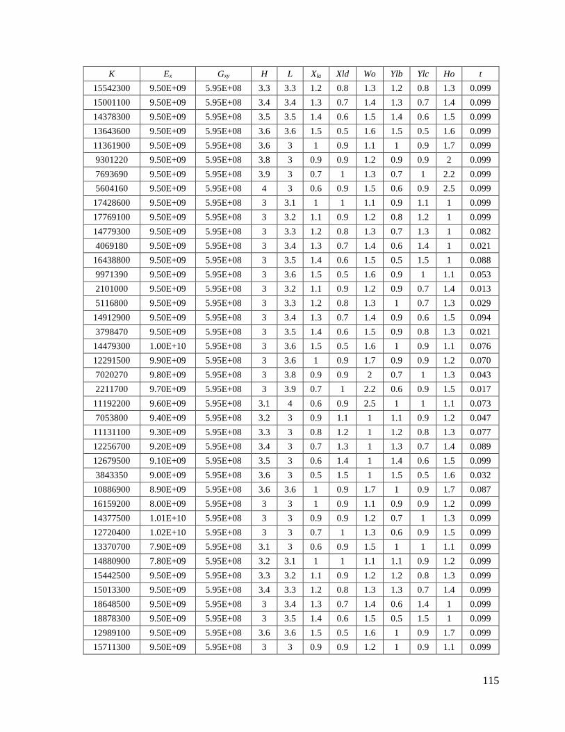
115
K Ex Gxy H L Xla Xld Wo Ylb Ylc Ho t
15542300 9.50E+09 5.95E+08 3.3 3.3 1.2 0.8 1.3 1.2 0.8 1.3 0.099
15001100 9.50E+09 5.95E+08 3.4 3.4 1.3 0.7 1.4 1.3 0.7 1.4 0.099
14378300 9.50E+09 5.95E+08 3.5 3.5 1.4 0.6 1.5 1.4 0.6 1.5 0.099
13643600 9.50E+09 5.95E+08 3.6 3.6 1.5 0.5 1.6 1.5 0.5 1.6 0.099
11361900 9.50E+09 5.95E+08 3.6 3 1 0.9 1.1 1 0.9 1.7 0.099
9301220 9.50E+09 5.95E+08 3.8 3 0.9 0.9 1.2 0.9 0.9 2 0.099
7693690 9.50E+09 5.95E+08 3.9 3 0.7 1 1.3 0.7 1 2.2 0.099
5604160 9.50E+09 5.95E+08 4 3 0.6 0.9 1.5 0.6 0.9 2.5 0.099
17428600 9.50E+09 5.95E+08 3 3.1 1 1 1.1 0.9 1.1 1 0.099
17769100 9.50E+09 5.95E+08 3 3.2 1.1 0.9 1.2 0.8 1.2 1 0.099
14779300 9.50E+09 5.95E+08 3 3.3 1.2 0.8 1.3 0.7 1.3 1 0.082
4069180 9.50E+09 5.95E+08 3 3.4 1.3 0.7 1.4 0.6 1.4 1 0.021
16438800 9.50E+09 5.95E+08 3 3.5 1.4 0.6 1.5 0.5 1.5 1 0.088
9971390 9.50E+09 5.95E+08 3 3.6 1.5 0.5 1.6 0.9 1 1.1 0.053
2101000 9.50E+09 5.95E+08 3 3.2 1.1 0.9 1.2 0.9 0.7 1.4 0.013
5116800 9.50E+09 5.95E+08 3 3.3 1.2 0.8 1.3 1 0.7 1.3 0.029
14912900 9.50E+09 5.95E+08 3 3.4 1.3 0.7 1.4 0.9 0.6 1.5 0.094
3798470 9.50E+09 5.95E+08 3 3.5 1.4 0.6 1.5 0.9 0.8 1.3 0.021
14479300 1.00E+10 5.95E+08 3 3.6 1.5 0.5 1.6 1 0.9 1.1 0.076
12291500 9.90E+09 5.95E+08 3 3.6 1 0.9 1.7 0.9 0.9 1.2 0.070
7020270 9.80E+09 5.95E+08 3 3.8 0.9 0.9 2 0.7 1 1.3 0.043
2211700 9.70E+09 5.95E+08 3 3.9 0.7 1 2.2 0.6 0.9 1.5 0.017
11192200 9.60E+09 5.95E+08 3.1 4 0.6 0.9 2.5 1 1 1.1 0.073
7053800 9.40E+09 5.95E+08 3.2 3 0.9 1.1 1 1.1 0.9 1.2 0.047
11131100 9.30E+09 5.95E+08 3.3 3 0.8 1.2 1 1.2 0.8 1.3 0.077
12256700 9.20E+09 5.95E+08 3.4 3 0.7 1.3 1 1.3 0.7 1.4 0.089
12679500 9.10E+09 5.95E+08 3.5 3 0.6 1.4 1 1.4 0.6 1.5 0.099
3843350 9.00E+09 5.95E+08 3.6 3 0.5 1.5 1 1.5 0.5 1.6 0.032
10886900 8.90E+09 5.95E+08 3.6 3.6 1 0.9 1.7 1 0.9 1.7 0.087
16159200 8.00E+09 5.95E+08 3 3 1 0.9 1.1 0.9 0.9 1.2 0.099
14377500 1.01E+10 5.95E+08 3 3 0.9 0.9 1.2 0.7 1 1.3 0.099
12720400 1.02E+10 5.95E+08 3 3 0.7 1 1.3 0.6 0.9 1.5 0.099
13370700 7.90E+09 5.95E+08 3.1 3 0.6 0.9 1.5 1 1 1.1 0.099
14880900 7.80E+09 5.95E+08 3.2 3.1 1 1 1.1 1.1 0.9 1.2 0.099
15442500 9.50E+09 5.95E+08 3.3 3.2 1.1 0.9 1.2 1.2 0.8 1.3 0.099
15013300 9.50E+09 5.95E+08 3.4 3.3 1.2 0.8 1.3 1.3 0.7 1.4 0.099
18648500 9.50E+09 5.95E+08 3 3.4 1.3 0.7 1.4 0.6 1.4 1 0.099
18878300 9.50E+09 5.95E+08 3 3.5 1.4 0.6 1.5 0.5 1.5 1 0.099
12989100 9.50E+09 5.95E+08 3.6 3.6 1.5 0.5 1.6 1 0.9 1.7 0.099
15711300 9.50E+09 5.95E+08 3 3 0.9 0.9 1.2 1 0.9 1.1 0.099

116
K Ex Gxy H L Xla Xld Wo Ylb Ylc Ho t
14380500 9.50E+09 5.95E+08 3 3 0.7 1 1.3 0.9 0.9 1.2 0.099
12202300 9.50E+09 5.95E+08 3 3 0.6 0.9 1.5 0.7 1 1.3 0.099
12492400 9.50E+09 5.95E+08 3 3.1 1 1 1.1 0.6 0.9 1.5 0.085
11738000 9.50E+09 5.95E+08 3.1 3.2 1.1 0.9 1.2 1 1 1.1 0.07
7289530 9.50E+09 5.95E+08 3.2 3.3 1.2 0.8 1.3 1.1 0.9 1.2 0.045
11692600 9.50E+09 5.95E+08 3.3 3.4 1.3 0.7 1.4 1.2 0.8 1.3 0.075
4023260 9.50E+09 5.95E+08 3.5 3.5 1.4 0.6 1.5 1.4 0.6 1.5 0.027
2103700 9.50E+09 5.95E+08 3.6 3.6 1.5 0.5 1.6 1.5 0.5 1.6 0.014
11524900 9.50E+09 5.95E+08 3.6 3.6 1 0.9 1.7 1 0.9 1.7 0.094
12066100 9.50E+09 6.00E+08 3 3 0.9 0.7 1.4 0.9 0.7 1.4 0.091
7117820 9.50E+09 6.10E+08 3 3 1 0.7 1.3 0.9 0.9 1.2 0.047
10621700 9.50E+09 6.20E+08 3 3 0.9 0.6 1.5 0.7 1 1.3 0.081
7152040 9.50E+09 6.30E+08 3 3 0.9 0.8 1.3 0.6 0.9 1.5 0.054
4658650 1.00E+10 6.40E+08 3.1 3 1 0.9 1.1 1 1 1.1 0.028
12434700 9.90E+09 6.50E+08 3.2 3 0.9 0.9 1.2 1.1 0.9 1.2 0.081
3292410 9.80E+09 6.90E+08 3.3 3 0.7 1 1.3 1.2 0.8 1.3 0.023
4680990 9.10E+09 7.00E+08 3.4 3.5 1.4 0.6 1.5 1.3 0.7 1.4 0.028
13717700 9.00E+09 5.50E+08 3.5 3.6 1.5 0.5 1.6 1.4 0.6 1.5 0.099
12504000 8.90E+09 5.40E+08 3.6 3.6 1 0.9 1.7 1.5 0.5 1.6 0.099
10402000 8.00E+09 5.70E+08 3.6 3 0.9 0.9 1.2 1 0.9 1.7 0.099
13409900 1.01E+10 5.80E+08 3 3 0.7 1 1.3 0.7 1 1.3 0.099
10183800 1.02E+10 5.00E+08 3 3 0.6 0.9 1.5 0.6 0.9 1.5 0.099
12344700 7.90E+09 4.50E+08 3.1 3.1 1 1 1.1 1 1 1.1 0.088
2168170 7.80E+09 8.00E+08 3.2 3.2 1.1 0.9 1.2 1.1 0.9 1.2 0.012
7146740 9.50E+09 3.00E+08 3.3 3.3 1.2 0.8 1.3 1.2 0.8 1.3 0.069
11176400 9.50E+09 4.40E+08 3.4 3.4 1.3 0.7 1.4 1.3 0.7 1.4 0.087
2364930 9.50E+09 4.10E+08 3.5 3.5 1.4 0.6 1.5 1.4 0.6 1.5 0.02
9245670 9.50E+09 7.20E+08 3.6 3.6 1.5 0.5 1.6 1.5 0.5 1.6 0.059
13976800 9.50E+09 7.30E+08 3.6 3.6 1 0.9 1.7 1 0.9 1.7 0.099
26032700 9.88E+09 6.06E+08 2.8 3.2 0.8 1.4 1 1.5 0.5 0.8 0.119
9212300 9.27E+09 5.77E+08 3.8 2.7 1 1.1 0.6 1.5 0.9 1.4 0.084
10295800 9.82E+09 5.54E+08 3.4 2.8 1 0.5 1.3 1.1 1.3 1 0.088
14671100 9.28E+09 5.94E+08 3.1 3.2 1.4 0.5 1.3 1 0.8 1.3 0.096
20178000 9.77E+09 5.68E+08 3.2 3.5 1.2 1.3 1 0.8 1.4 1 0.107
25214400 9.74E+09 5.36E+08 2.7 3.7 1.3 1.5 0.9 0.7 0.7 1.3 0.113
19776100 1.02E+10 6.40E+08 3 3.2 1 1.5 0.7 0.5 1.2 1.3 0.101
20698400 8.88E+09 5.33E+08 3.2 3.6 1.4 1.5 0.7 0.9 1.3 1 0.102
10959100 8.71E+09 6.13E+08 3.5 2.8 1.1 1 0.7 1 1.4 1.1 0.082
17776600 1.02E+10 6.14E+08 2.3 2.1 0.5 0.9 0.7 1.1 0.5 0.7 0.106
19850500 9.37E+09 5.88E+08 2.8 3.3 0.9 1.2 1.2 0.9 0.7 1.2 0.104
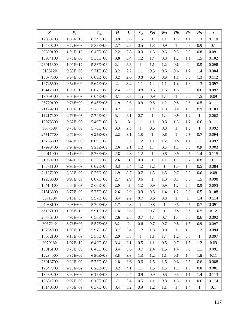
117
K Ex Gxy H L Xla Xld Wo Ylb Ylc Ho t
19063700 1.00E+10 6.34E+08 3.9 3.6 1.5 1 1.1 1.5 1.1 1.3 0.119
16480200 9.77E+09 5.33E+08 2.7 2.7 0.5 1.3 0.9 1 0.8 0.9 0.1
23800100 1.01E+10 6.40E+08 2.2 2.8 0.9 1.3 0.6 0.5 0.9 0.8 0.091
13984100 8.75E+09 5.38E+08 3.8 3.4 1.2 1.4 0.8 1.2 1.1 1.5 0.102
28911800 1.01E+10 5.86E+08 2.1 3.3 1 1.1 1.2 0.6 1 0.5 0.098
8105220 9.33E+09 5.71E+08 3.2 2.2 1.1 0.5 0.6 0.6 1.2 1.4 0.084
13877500 9.94E+09 6.09E+08 3.2 2.6 0.8 0.9 0.9 1.1 0.8 1.3 0.112
12745500 9.54E+09 5.67E+08 4 3.4 1.1 1.2 1.1 1.4 1.3 1.3 0.097
19417800 1.01E+10 6.07E+08 2.4 2.9 0.8 0.6 1.5 1.3 0.5 0.6 0.092
17009500 9.04E+09 6.04E+08 3.1 3.8 1.5 0.9 1.4 1 0.6 1.5 0.09
28779100 9.76E+09 6.48E+08 1.9 2.6 0.9 0.5 1.2 0.8 0.6 0.5 0.111
21199200 1.02E+10 5.78E+08 3.2 3.8 1.1 1.4 1.3 0.8 1.5 0.9 0.103
12217300 8.73E+09 5.78E+08 3.1 3.1 0.7 1 1.4 0.9 1.2 1 0.082
18978500 9.32E+09 5.49E+08 3.1 3 1.1 1.1 0.8 1.3 1.2 0.6 0.111
9677690 9.78E+09 5.78E+08 3.3 2.3 1 0.5 0.8 1 1.3 1 0.092
27517700 9.79E+09 6.25E+08 2.2 3.1 1.5 1 0.6 1 0.5 0.7 0.094
19785800 9.45E+09 6.09E+08 3 3.5 1.2 1.1 1.2 0.8 1.1 1.1 0.097
17990400 8.94E+09 5.32E+08 2.6 3.1 1.2 1.4 0.5 1.2 0.5 0.9 0.082
20011000 9.14E+09 5.76E+08 2.8 2.8 1.2 1 0.6 0.9 0.5 1.4 0.115
21989200 9.47E+09 6.36E+08 2.6 3 0.9 1 1.1 1.1 0.7 0.8 0.1
16771100 9.91E+09 6.02E+08 3.3 3.4 1.2 1.2 1 1.5 1.3 0.5 0.084
24127200 8.83E+09 5.76E+08 1.9 3.7 0.7 1.5 1.5 0.7 0.6 0.6 0.08
12288800 9.91E+09 6.07E+08 2.7 2.9 0.6 1 1.3 0.7 0.5 1.5 0.098
16514100 8.84E+09 5.64E+08 2.9 3 1.2 0.9 0.9 1.2 0.8 0.9 0.093
21513800 8.77E+09 5.75E+08 2.6 2.9 0.9 0.6 1.4 1.2 0.9 0.5 0.108
8571390 9.10E+09 5.57E+08 3.4 2.2 0.7 0.6 0.9 1 1 1.4 0.114
24933100 9.98E+09 5.70E+08 1.7 2.8 1 0.8 1 0.5 0.5 0.7 0.091
36197100 1.03E+10 5.91E+08 1.8 2.8 1.1 0.7 1 0.8 0.5 0.5 0.12
20386700 8.96E+09 6.50E+08 2.6 2.8 0.7 1.4 0.7 1.4 0.6 0.6 0.092
8067240 8.76E+09 5.57E+08 3.2 2 0.6 0.7 0.7 0.8 1.5 0.9 0.097
15254900 1.03E+10 5.97E+08 3.7 3.4 1.2 1.3 0.9 1 1.5 1.2 0.094
18632100 9.11E+09 5.55E+08 2.9 3.5 1 1.1 1.4 1.2 0.7 1 0.097
8070180 1.02E+10 6.42E+08 3.4 2.1 0.5 1.1 0.5 0.7 1.5 1.2 0.09
16016100 9.73E+09 6.46E+08 3.4 3.6 0.7 1.4 1.5 1.4 0.9 1.1 0.091
19234000 9.87E+09 6.50E+08 3.5 3.6 1.3 1.2 1.1 0.6 1.4 1.5 0.11
26013700 9.21E+09 5.73E+08 1.8 3.6 0.6 1.5 1.5 0.6 0.6 0.6 0.088
19547800 9.37E+09 6.20E+08 3.2 4.1 1.1 1.5 1.5 1.2 1.2 0.8 0.081
13459200 8.92E+09 6.15E+08 3 2.4 0.9 0.9 0.6 0.5 1.1 1.4 0.113
15681200 9.92E+09 6.13E+08 3 2.4 0.5 1.1 0.8 1.3 1.1 0.6 0.114
16140300 8.76E+09 6.37E+08 3.4 3.2 0.9 1.2 1.1 1 1.4 1 0.1
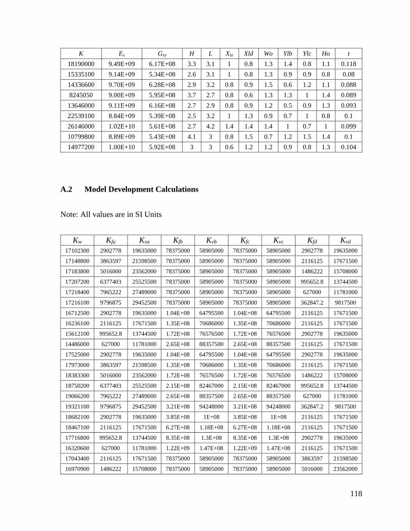
118
K Ex Gxy H L Xla Xld Wo Ylb Ylc Ho t
18190000 9.49E+09 6.17E+08 3.3 3.1 1 0.8 1.3 1.4 0.8 1.1 0.118
15335100 9.14E+09 5.34E+08 2.6 3.1 1 0.8 1.3 0.9 0.9 0.8 0.08
14336600 9.70E+09 6.28E+08 2.9 3.2 0.8 0.9 1.5 0.6 1.2 1.1 0.088
8245050 9.00E+09 5.95E+08 3.7 2.7 0.8 0.6 1.3 1.3 1 1.4 0.089
13646000 9.11E+09 6.16E+08 2.7 2.9 0.8 0.9 1.2 0.5 0.9 1.3 0.093
22539100 8.84E+09 5.39E+08 2.5 3.2 1 1.3 0.9 0.7 1 0.8 0.1
26146000 1.02E+10 5.61E+08 2.7 4.2 1.4 1.4 1.4 1 0.7 1 0.099
10799800 8.89E+09 5.43E+08 4.1 3 0.8 1.5 0.7 1.2 1.5 1.4 0.1
14977200 1.00E+10 5.92E+08 3 3 0.6 1.2 1.2 0.9 0.8 1.3 0.104
A.2 Model Development Calculations
Note: All values are in SI Units
Kw Kfa Kva Kfb Kvb Kfc Kvc Kfd Kvd
17102300 2902778 19635000 78375000 58905000 78375000 58905000 2902778 19635000
17148800 3863597 21598500 78375000 58905000 78375000 58905000 2116125 17671500
17183800 5016000 23562000 78375000 58905000 78375000 58905000 1486222 15708000
17207200 6377403 25525500 78375000 58905000 78375000 58905000 995652.8 13744500
17218400 7965222 27489000 78375000 58905000 78375000 58905000 627000 11781000
17216100 9796875 29452500 78375000 58905000 78375000 58905000 362847.2 9817500
16712500 2902778 19635000 1.04E+08 64795500 1.04E+08 64795500 2116125 17671500
16236100 2116125 17671500 1.35E+08 70686000 1.35E+08 70686000 2116125 17671500
15612100 995652.8 13744500 1.72E+08 76576500 1.72E+08 76576500 2902778 19635000
14486000 627000 11781000 2.65E+08 88357500 2.65E+08 88357500 2116125 17671500
17525000 2902778 19635000 1.04E+08 64795500 1.04E+08 64795500 2902778 19635000
17973000 3863597 21598500 1.35E+08 70686000 1.35E+08 70686000 2116125 17671500
18383300 5016000 23562000 1.72E+08 76576500 1.72E+08 76576500 1486222 15708000
18750200 6377403 25525500 2.15E+08 82467000 2.15E+08 82467000 995652.8 13744500
19066200 7965222 27489000 2.65E+08 88357500 2.65E+08 88357500 627000 11781000
19321100 9796875 29452500 3.21E+08 94248000 3.21E+08 94248000 362847.2 9817500
18682100 2902778 19635000 3.85E+08 1E+08 3.85E+08 1E+08 2116125 17671500
18467100 2116125 17671500 6.27E+08 1.18E+08 6.27E+08 1.18E+08 2116125 17671500
17716800 995652.8 13744500 8.35E+08 1.3E+08 8.35E+08 1.3E+08 2902778 19635000
16320600 627000 11781000 1.22E+09 1.47E+08 1.22E+09 1.47E+08 2116125 17671500
17043400 2116125 17671500 78375000 58905000 78375000 58905000 3863597 21598500
16970900 1486222 15708000 78375000 58905000 78375000 58905000 5016000 23562000
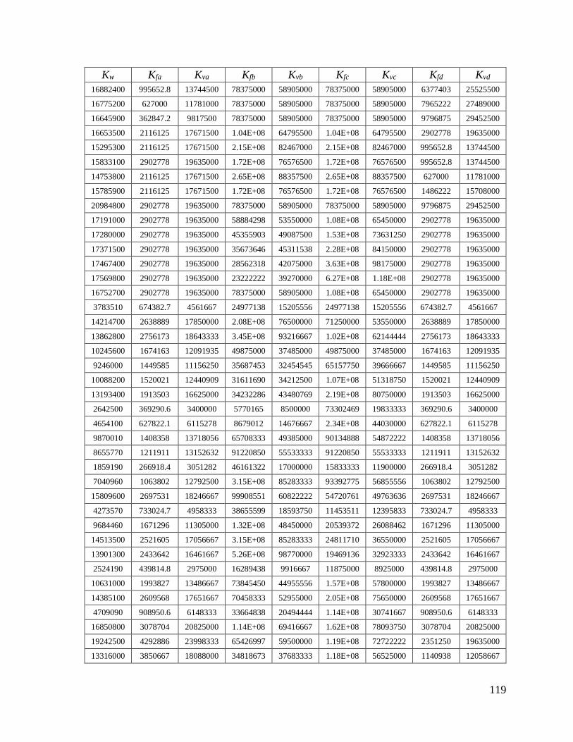
119
Kw Kfa Kva Kfb Kvb Kfc Kvc Kfd Kvd
16882400 995652.8 13744500 78375000 58905000 78375000 58905000 6377403 25525500
16775200 627000 11781000 78375000 58905000 78375000 58905000 7965222 27489000
16645900 362847.2 9817500 78375000 58905000 78375000 58905000 9796875 29452500
16653500 2116125 17671500 1.04E+08 64795500 1.04E+08 64795500 2902778 19635000
15295300 2116125 17671500 2.15E+08 82467000 2.15E+08 82467000 995652.8 13744500
15833100 2902778 19635000 1.72E+08 76576500 1.72E+08 76576500 995652.8 13744500
14753800 2116125 17671500 2.65E+08 88357500 2.65E+08 88357500 627000 11781000
15785900 2116125 17671500 1.72E+08 76576500 1.72E+08 76576500 1486222 15708000
20984800 2902778 19635000 78375000 58905000 78375000 58905000 9796875 29452500
17191000 2902778 19635000 58884298 53550000 1.08E+08 65450000 2902778 19635000
17280000 2902778 19635000 45355903 49087500 1.53E+08 73631250 2902778 19635000
17371500 2902778 19635000 35673646 45311538 2.28E+08 84150000 2902778 19635000
17467400 2902778 19635000 28562318 42075000 3.63E+08 98175000 2902778 19635000
17569800 2902778 19635000 23222222 39270000 6.27E+08 1.18E+08 2902778 19635000
16752700 2902778 19635000 78375000 58905000 1.08E+08 65450000 2902778 19635000
3783510 674382.7 4561667 24977138 15205556 24977138 15205556 674382.7 4561667
14214700 2638889 17850000 2.08E+08 76500000 71250000 53550000 2638889 17850000
13862800 2756173 18643333 3.45E+08 93216667 1.02E+08 62144444 2756173 18643333
10245600 1674163 12091935 49875000 37485000 49875000 37485000 1674163 12091935
9246000 1449585 11156250 35687453 32454545 65157750 39666667 1449585 11156250
10088200 1520021 12440909 31611690 34212500 1.07E+08 51318750 1520021 12440909
13193400 1913503 16625000 34232286 43480769 2.19E+08 80750000 1913503 16625000
2642500 369290.6 3400000 5770165 8500000 73302469 19833333 369290.6 3400000
4654100 627822.1 6115278 8679012 14676667 2.34E+08 44030000 627822.1 6115278
9870010 1408358 13718056 65708333 49385000 90134888 54872222 1408358 13718056
8655770 1211911 13152632 91220850 55533333 91220850 55533333 1211911 13152632
1859190 266918.4 3051282 46161322 17000000 15833333 11900000 266918.4 3051282
7040960 1063802 12792500 3.15E+08 85283333 93392775 56855556 1063802 12792500
15809600 2697531 18246667 99908551 60822222 54720761 49763636 2697531 18246667
4273570 733024.7 4958333 38655599 18593750 11453511 12395833 733024.7 4958333
9684460 1671296 11305000 1.32E+08 48450000 20539372 26088462 1671296 11305000
14513500 2521605 17056667 3.15E+08 85283333 24811710 36550000 2521605 17056667
13901300 2433642 16461667 5.26E+08 98770000 19469136 32923333 2433642 16461667
2524190 439814.8 2975000 16289438 9916667 11875000 8925000 439814.8 2975000
10631000 1993827 13486667 73845450 44955556 1.57E+08 57800000 1993827 13486667
14385100 2609568 17651667 70458333 52955000 2.05E+08 75650000 2609568 17651667
4709090 908950.6 6148333 33664838 20494444 1.14E+08 30741667 908950.6 6148333
16850800 3078704 20825000 1.14E+08 69416667 1.62E+08 78093750 3078704 20825000
19242500 4292886 23998333 65426997 59500000 1.19E+08 72722222 2351250 19635000
13316000 3850667 18088000 34818673 37683333 1.18E+08 56525000 1140938 12058667
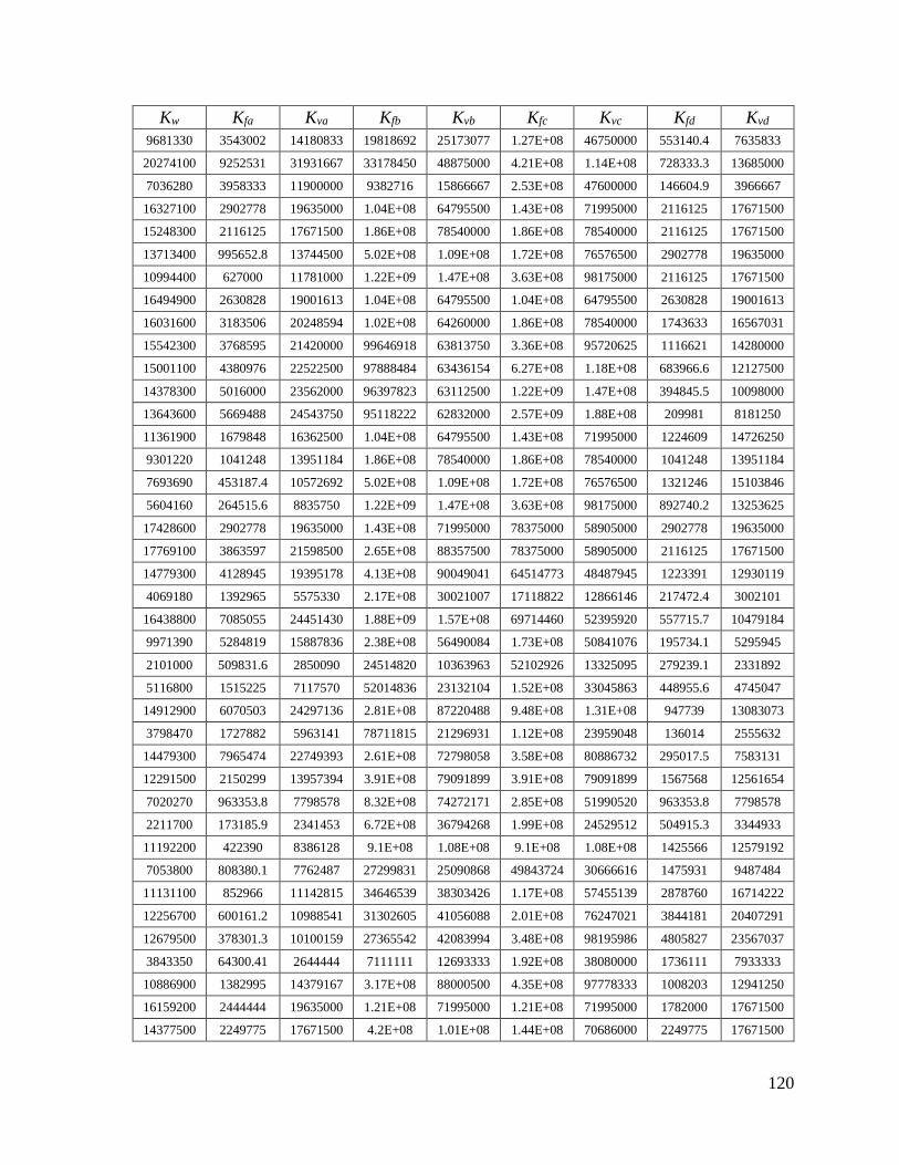
120
Kw Kfa Kva Kfb Kvb Kfc Kvc Kfd Kvd
9681330 3543002 14180833 19818692 25173077 1.27E+08 46750000 553140.4 7635833
20274100 9252531 31931667 33178450 48875000 4.21E+08 1.14E+08 728333.3 13685000
7036280 3958333 11900000 9382716 15866667 2.53E+08 47600000 146604.9 3966667
16327100 2902778 19635000 1.04E+08 64795500 1.43E+08 71995000 2116125 17671500
15248300 2116125 17671500 1.86E+08 78540000 1.86E+08 78540000 2116125 17671500
13713400 995652.8 13744500 5.02E+08 1.09E+08 1.72E+08 76576500 2902778 19635000
10994400 627000 11781000 1.22E+09 1.47E+08 3.63E+08 98175000 2116125 17671500
16494900 2630828 19001613 1.04E+08 64795500 1.04E+08 64795500 2630828 19001613
16031600 3183506 20248594 1.02E+08 64260000 1.86E+08 78540000 1743633 16567031
15542300 3768595 21420000 99646918 63813750 3.36E+08 95720625 1116621 14280000
15001100 4380976 22522500 97888484 63436154 6.27E+08 1.18E+08 683966.6 12127500
14378300 5016000 23562000 96397823 63112500 1.22E+09 1.47E+08 394845.5 10098000
13643600 5669488 24543750 95118222 62832000 2.57E+09 1.88E+08 209981 8181250
11361900 1679848 16362500 1.04E+08 64795500 1.43E+08 71995000 1224609 14726250
9301220 1041248 13951184 1.86E+08 78540000 1.86E+08 78540000 1041248 13951184
7693690 453187.4 10572692 5.02E+08 1.09E+08 1.72E+08 76576500 1321246 15103846
5604160 264515.6 8835750 1.22E+09 1.47E+08 3.63E+08 98175000 892740.2 13253625
17428600 2902778 19635000 1.43E+08 71995000 78375000 58905000 2902778 19635000
17769100 3863597 21598500 2.65E+08 88357500 78375000 58905000 2116125 17671500
14779300 4128945 19395178 4.13E+08 90049041 64514773 48487945 1223391 12930119
4069180 1392965 5575330 2.17E+08 30021007 17118822 12866146 217472.4 3002101
16438800 7085055 24451430 1.88E+09 1.57E+08 69714460 52395920 557715.7 10479184
9971390 5284819 15887836 2.38E+08 56490084 1.73E+08 50841076 195734.1 5295945
2101000 509831.6 2850090 24514820 10363963 52102926 13325095 279239.1 2331892
5116800 1515225 7117570 52014836 23132104 1.52E+08 33045863 448955.6 4745047
14912900 6070503 24297136 2.81E+08 87220488 9.48E+08 1.31E+08 947739 13083073
3798470 1727882 5963141 78711815 21296931 1.12E+08 23959048 136014 2555632
14479300 7965474 22749393 2.61E+08 72798058 3.58E+08 80886732 295017.5 7583131
12291500 2150299 13957394 3.91E+08 79091899 3.91E+08 79091899 1567568 12561654
7020270 963353.8 7798578 8.32E+08 74272171 2.85E+08 51990520 963353.8 7798578
2211700 173185.9 2341453 6.72E+08 36794268 1.99E+08 24529512 504915.3 3344933
11192200 422390 8386128 9.1E+08 1.08E+08 9.1E+08 1.08E+08 1425566 12579192
7053800 808380.1 7762487 27299831 25090868 49843724 30666616 1475931 9487484
11131100 852966 11142815 34646539 38303426 1.17E+08 57455139 2878760 16714222
12256700 600161.2 10988541 31302605 41056088 2.01E+08 76247021 3844181 20407291
12679500 378301.3 10100159 27365542 42083994 3.48E+08 98195986 4805827 23567037
3843350 64300.41 2644444 7111111 12693333 1.92E+08 38080000 1736111 7933333
10886900 1382995 14379167 3.17E+08 88000500 4.35E+08 97778333 1008203 12941250
16159200 2444444 19635000 1.21E+08 71995000 1.21E+08 71995000 1782000 17671500
14377500 2249775 17671500 4.2E+08 1.01E+08 1.44E+08 70686000 2249775 17671500
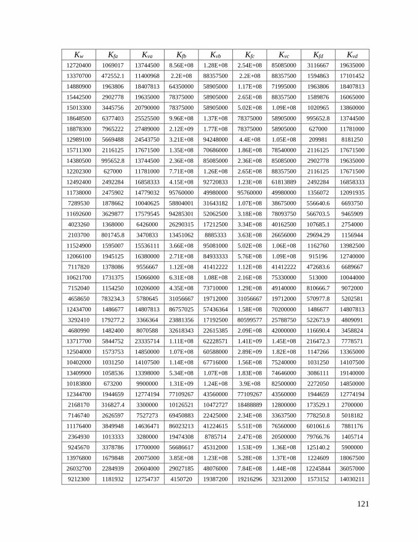
121
Kw Kfa Kva Kfb Kvb Kfc Kvc Kfd Kvd
12720400 1069017 13744500 8.56E+08 1.28E+08 2.54E+08 85085000 3116667 19635000
13370700 472552.1 11400968 2.2E+08 88357500 2.2E+08 88357500 1594863 17101452
14880900 1963806 18407813 64350000 58905000 1.17E+08 71995000 1963806 18407813
15442500 2902778 19635000 78375000 58905000 2.65E+08 88357500 1589876 16065000
15013300 3445756 20790000 78375000 58905000 5.02E+08 1.09E+08 1020965 13860000
18648500 6377403 25525500 9.96E+08 1.37E+08 78375000 58905000 995652.8 13744500
18878300 7965222 27489000 2.12E+09 1.77E+08 78375000 58905000 627000 11781000
12989100 5669488 24543750 3.21E+08 94248000 4.4E+08 1.05E+08 209981 8181250
15711300 2116125 17671500 1.35E+08 70686000 1.86E+08 78540000 2116125 17671500
14380500 995652.8 13744500 2.36E+08 85085000 2.36E+08 85085000 2902778 19635000
12202300 627000 11781000 7.71E+08 1.26E+08 2.65E+08 88357500 2116125 17671500
12492400 2492284 16858333 4.15E+08 92720833 1.23E+08 61813889 2492284 16858333
11738000 2475902 14779032 95760000 49980000 95760000 49980000 1356072 12091935
7289530 1878662 10040625 58804001 31643182 1.07E+08 38675000 556640.6 6693750
11692600 3629877 17579545 94285301 52062500 3.18E+08 78093750 566703.5 9465909
4023260 1368000 6426000 26290315 17212500 3.34E+08 40162500 107685.1 2754000
2103700 801745.8 3470833 13451062 8885333 3.63E+08 26656000 29694.29 1156944
11524900 1595007 15536111 3.66E+08 95081000 5.02E+08 1.06E+08 1162760 13982500
12066100 1945125 16380000 2.71E+08 84933333 5.76E+08 1.09E+08 915196 12740000
7117820 1378086 9556667 1.12E+08 41412222 1.12E+08 41412222 472683.6 6689667
10621700 1731375 15066000 6.31E+08 1.08E+08 2.16E+08 75330000 513000 10044000
7152040 1154250 10206000 4.35E+08 73710000 1.29E+08 49140000 810666.7 9072000
4658650 783234.3 5780645 31056667 19712000 31056667 19712000 570977.8 5202581
12434700 1486677 14807813 86757025 57436364 1.58E+08 70200000 1486677 14807813
3292410 179277.2 3366364 23881356 17192500 80599577 25788750 522673.9 4809091
4680990 1482400 8070588 32618343 22615385 2.09E+08 42000000 116690.4 3458824
13717700 5844752 23335714 1.11E+08 62228571 1.41E+09 1.45E+08 216472.3 7778571
12504000 1573753 14850000 1.07E+08 60588000 2.89E+09 1.82E+08 1147266 13365000
10402000 1031250 14107500 1.14E+08 67716000 1.56E+08 75240000 1031250 14107500
13409900 1058536 13398000 5.34E+08 1.07E+08 1.83E+08 74646000 3086111 19140000
10183800 673200 9900000 1.31E+09 1.24E+08 3.9E+08 82500000 2272050 14850000
12344700 1944659 12774194 77109267 43560000 77109267 43560000 1944659 12774194
2168170 316827.4 3300000 10126521 10472727 18488889 12800000 173529.1 2700000
7146740 2626597 7527273 69450883 22425000 2.34E+08 33637500 778250.8 5018182
11176400 3849948 14636471 86023213 41224615 5.51E+08 76560000 601061.6 7881176
2364930 1013333 3280000 19474308 8785714 2.47E+08 20500000 79766.76 1405714
9245670 3378786 17700000 56686617 45312000 1.53E+09 1.36E+08 125140.2 5900000
13976800 1679848 20075000 3.85E+08 1.23E+08 5.28E+08 1.37E+08 1224609 18067500
26032700 2284939 20604000 29027185 48076000 7.84E+08 1.44E+08 12245844 36057000
9212300 1181932 12754737 4150720 19387200 19216296 32312000 1573152 14030211

122
Kw Kfa Kva Kfb Kvb Kfc Kvc Kfd Kvd
10295800 1831841 14338824 1.19E+08 57616000 71998667 48752000 228980.1 7169412
14671100 6840335 25752774 1.63E+08 74131200 3.19E+08 92664000 311604.2 9197419
20178000 4594469 22791000 1.7E+08 75970000 31751002 43411429 5841463 24690250
25214400 10236473 29162370 1.95E+08 77873143 1.95E+08 77873143 15725123 33648889
19776100 3174330 21546667 2.35E+08 90496000 17012426 37706667 10713365 32320000
20698400 6320713 23785125 35513909 42284667 11784087 29274000 7774200 25484063
10959100 1847671 15797886 20414788 35186200 7439792 25133000 1388183 14361714
17776600 922937 14148696 23150567 41417091 2.47E+08 91117600 5382569 25467652
19850500 2697641 19656000 1.93E+08 81536000 4.09E+08 1.05E+08 6394408 26208000
19063700 5648370 29017692 39151414 55327067 99275750 75446000 1673591 19345128
16480200 516996.5 9870370 59346675 47970000 1.16E+08 59962500 9086730 25662963
23800100 5238546 23825455 1.32E+08 69888000 22671358 38826667 15787499 34414545
13984100 2341375 17329263 22029481 36584000 28600258 39909818 3718017 20217474
28911800 8890653 27346667 6.59E+08 1.15E+08 1.42E+08 68913600 11833459 30081333
8105220 2652251 16487625 65296000 47964000 8162000 23982000 249084.5 7494375
13877500 1449729 17052000 50817854 55806545 1.32E+08 76734000 2064165 19183500
12745500 1602910 15124725 37385667 43213500 46693796 46537615 2081014 16499700
19417800 2861654 18614667 1.19E+08 64435385 2.09E+09 1.68E+08 1207260 13961000
17009500 7681011 26303226 1.86E+08 76104000 8.61E+08 1.27E+08 1659098 15781935
28779100 9599226 34071158 3.05E+08 1.08E+08 7.23E+08 1.44E+08 1645958 18928421
21199200 3566992 20464813 3.77E+08 96742750 57165018 51596133 7353739 26046125
12217300 687155.2 10702323 2.25E+08 73727111 94773335 55295333 2003368 15289032
18978500 3851684 21623516 20090815 37500923 25543704 40626000 3851684 21623516
9677690 2086002 16113939 38381909 42540800 17470145 32723692 260750.3 8056970
27517700 24304723 40056818 16562988 35250000 1.33E+08 70500000 7201399 26704545
19785800 4886731 23629200 2.58E+08 88609500 99129773 64443273 3764027 21660100
17990400 6005446 20134154 4418632 18176667 61083167 43624000 9536425 23489846
20011000 6892708 28388571 25944568 44160000 1.51E+08 79488000 3988835 23657143
21989200 3272536 22015385 78900000 63600000 3.06E+08 99942857 4489076 24461538
16771100 3336944 18388364 20562370 33712000 31587619 38898462 3336944 18388364
24127200 2942096 16976842 5.79E+08 98742857 9.19E+08 1.15E+08 28949191 36378947
12288800 887959.8 13219111 5.18E+08 1.1E+08 1.42E+09 1.55E+08 4110925 22031852
16514100 4851299 21704276 28886309 39339000 97491292 59008500 2046642 16278207
21513800 3272661 21496154 1.25E+08 72450000 2.97E+08 96600000 969677.3 14330769
8571390 754021.4 13073118 62987423 57148200 62987423 57148200 474835.6 11205529
24933100 15404369 30511765 6.05E+08 1.04E+08 6.05E+08 1.04E+08 7887037 24409412
36197100 23470514 43340000 2.01E+08 88650000 8.23E+08 1.42E+08 6048374 27580000
20386700 1340418 16100000 8585708 29900000 1.09E+08 69766667 10723343 32200000
8067240 466498.7 10130438 47410092 47275375 7192287 25213533 740782.7 11818844
15254900 2745521 18200432 58669677 50506200 17383608 33670800 3490688 19717135
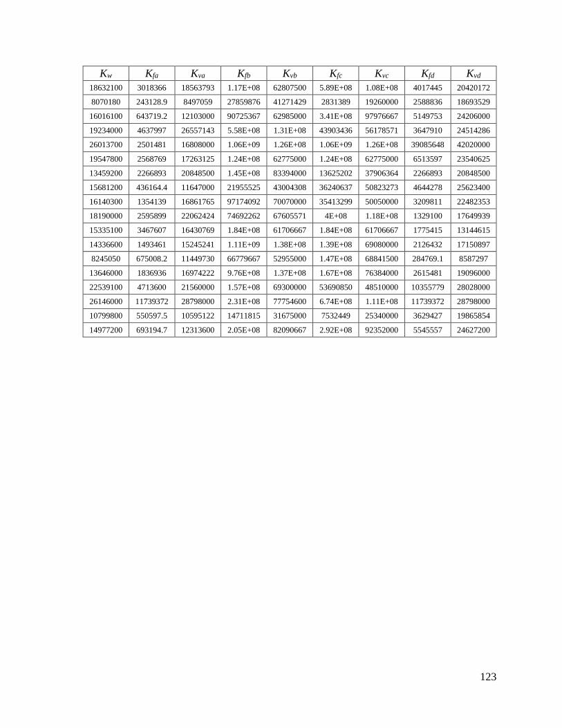
123
Kw Kfa Kva Kfb Kvb Kfc Kvc Kfd Kvd
18632100 3018366 18563793 1.17E+08 62807500 5.89E+08 1.08E+08 4017445 20420172
8070180 243128.9 8497059 27859876 41271429 2831389 19260000 2588836 18693529
16016100 643719.2 12103000 90725367 62985000 3.41E+08 97976667 5149753 24206000
19234000 4637997 26557143 5.58E+08 1.31E+08 43903436 56178571 3647910 24514286
26013700 2501481 16808000 1.06E+09 1.26E+08 1.06E+09 1.26E+08 39085648 42020000
19547800 2568769 17263125 1.24E+08 62775000 1.24E+08 62775000 6513597 23540625
13459200 2266893 20848500 1.45E+08 83394000 13625202 37906364 2266893 20848500
15681200 436164.4 11647000 21955525 43004308 36240637 50823273 4644278 25623400
16140300 1354139 16861765 97174092 70070000 35413299 50050000 3209811 22482353
18190000 2595899 22062424 74692262 67605571 4E+08 1.18E+08 1329100 17649939
15335100 3467607 16430769 1.84E+08 61706667 1.84E+08 61706667 1775415 13144615
14336600 1493461 15245241 1.11E+09 1.38E+08 1.39E+08 69080000 2126432 17150897
8245050 675008.2 11449730 66779667 52955000 1.47E+08 68841500 284769.1 8587297
13646000 1836936 16974222 9.76E+08 1.37E+08 1.67E+08 76384000 2615481 19096000
22539100 4713600 21560000 1.57E+08 69300000 53690850 48510000 10355779 28028000
26146000 11739372 28798000 2.31E+08 77754600 6.74E+08 1.11E+08 11739372 28798000
10799800 550597.5 10595122 14711815 31675000 7532449 25340000 3629427 19865854
14977200 693194.7 12313600 2.05E+08 82090667 2.92E+08 92352000 5545557 24627200