1

Forced Vibration of a Built-In Beam

Arnold Mukuvare

Group A1

Demonstrator: S. Mahabadi

SMOR: Dr N. Rockliff

Work carried out: April 24th

2013

Report completed: May 9th

2013

Abstract:

Forced vibration analysis is a very important phenomenon; these vibrations can give rise to a

lot of potential problems especially if the excitation force is periodic. The dynamic force can

either be externally applied or internally applied like the rotating machines. Oscillations can

be obtained from these vibrations and since all objects have a natural frequency which if the

forcing frequency reaches the system begins to oscillate with high amplitudes. The report is

taking the force to be a harmonic type ( ) Natural frequency results can be found in

many engineering tables but also can be determined experimentally or through calculations.

Theoretically it is shown in the report that the natural frequency is dependent on the Young’s

Modulus, length, breath, width and the total mass of that particular system. To investigate the

natural frequency a motor is used alongside with oscilloscopes to measure the circular

frequency and the amplitude relations. An error of 2.93% was obtained between the value of

the theoretical and experimental natural frequencies. Improvements could be made to this

experiment but the method proves to be a reliable way of predicting the value of the natural

frequency.

2

Contents

INTRODUCTION: ............................................................................................................................. 3

THEORY: ........................................................................................................................................... 3

PROCEDURES AND EQUIPMENT: ................................................................................................ 5

RESULTS: .......................................................................................................................................... 7

DISCUSSION: .................................................................................................................................... 9

CONCLUSION: ................................................................................................................................ 10

REFERENCES: ................................................................................................................................ 11

APPENDIX: ...................................................................................................................................... 12

3

INTRODUCTION:

One of the most common phenomena in engineering is the vibration of structures; there have

been many recorded failures of engineering systems as a result of not meeting excessive

vibration targets. In general if a dynamic system is acted upon by an applied external

harmonic force, the system begins to oscillate as a result. The oscillations can result in larger

amplitudes at certain frequency even at low periodic external forces. If the vibrations are such

that the frequency of the harmonic force is equal to the natural frequency of that particular

system then the system’s vibrations become excessive producing high amplitudes. This

phenomenon is known as resonance. The catastrophic collapse of the Tacoma Narrows

Bridge in 1940 shook engineers. At the time the most modern suspension bridge had failed as

a result of a light wind that caused the frequency of the vibrations to reach the bridge’s

natural frequency. On the day the bridge began to oscillate at exaggerated amplitudes and

collapsed.

Experimentally applying different frequencies to a system can give the natural frequency as

shown in figure (1). In this lab the frequency was found by using simple mass on a spring

analysis, changing the circular frequencies using a motor supported by a fixed beam.

Resonance can be obtained by the continued increase in the natural frequency which would

result in an increase in the amplitude from the oscillations.

It is worth noting that there are many several vibration types like (Free, Forced, Undamped

and Damped, Linear and Non-linear, and Deterministic and Random) vibrations. The

harmonic oscillations in this paper are induced by a periodic electric motor and are calculated

as Single Degree Of Freedom (SDOF).

THEORY:

The simplest system that can be used to demonstrate the steady state response of a single

degree of freedom oscillator is a mass on a spring system. (Nashif A.D., Jones D.I.G.,

Henderson J.P., 1985). An equation of motion can be considered in the analysis having

considered damping, acceleration and the spring constant. If a steady state harmonic

excitation is applied on the system would vibrate at amplitudes relating to the applied force’s

frequencies. Resonance will only be obtained only when the frequency from the excitation

force has reached the natural frequency of the system. The amplitudes of different forcing

frequencies can be decreased depending on the amount of damping that is available. The

presence of damping means that the maximum amplitude ratio occurs at a frequency lower

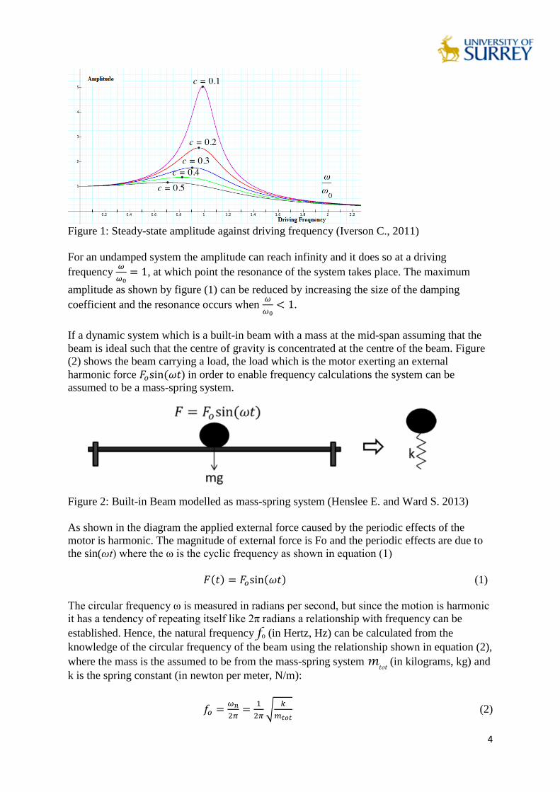
than the resonant frequency. Figure (1) shows the amplitude as a function of driving

frequency at different damping ratios ζ.

4

Figure 1: Steady-state amplitude against driving frequency (Iverson C., 2011)

For an undamped system the amplitude can reach infinity and it does so at a driving

frequency

, at which point the resonance of the system takes place. The maximum

amplitude as shown by figure (1) can be reduced by increasing the size of the damping

coefficient and the resonance occurs when

.

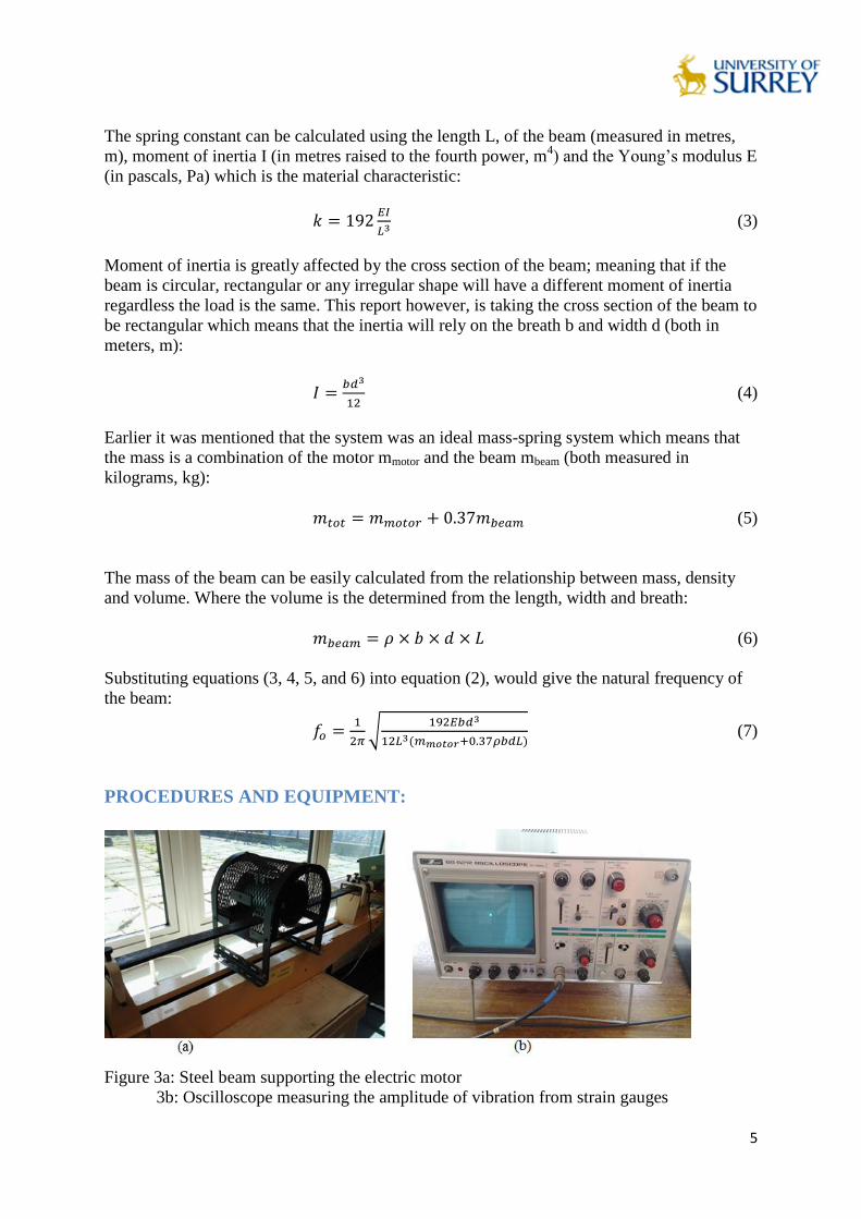
If a dynamic system which is a built-in beam with a mass at the mid-span assuming that the

beam is ideal such that the centre of gravity is concentrated at the centre of the beam. Figure

(2) shows the beam carrying a load, the load which is the motor exerting an external

harmonic force ( ) in order to enable frequency calculations the system can be

assumed to be a mass-spring system.

Figure 2: Built-in Beam modelled as mass-spring system (Henslee E. and Ward S. 2013)

As shown in the diagram the applied external force caused by the periodic effects of the

motor is harmonic. The magnitude of external force is Fo and the periodic effects are due to

the sin(ωt) where the ω is the cyclic frequency as shown in equation (1)

( ) ( ) (1)

The circular frequency ω is measured in radians per second, but since the motion is harmonic

it has a tendency of repeating itself like 2π radians a relationship with frequency can be

established. Hence, the natural frequency fo (in Hertz, Hz) can be calculated from the

knowledge of the circular frequency of the beam using the relationship shown in equation (2),

where the mass is the assumed to be from the mass-spring system mtot

(in kilograms, kg) and

k is the spring constant (in newton per meter, N/m):

√

(2)

5

The spring constant can be calculated using the length L, of the beam (measured in metres,

m), moment of inertia I (in metres raised to the fourth power, m4) and the Young’s modulus E

(in pascals, Pa) which is the material characteristic:

(3)

Moment of inertia is greatly affected by the cross section of the beam; meaning that if the

beam is circular, rectangular or any irregular shape will have a different moment of inertia

regardless the load is the same. This report however, is taking the cross section of the beam to

be rectangular which means that the inertia will rely on the breath b and width d (both in

meters, m):

(4)

Earlier it was mentioned that the system was an ideal mass-spring system which means that

the mass is a combination of the motor mmotor and the beam mbeam (both measured in

kilograms, kg):

(5)

The mass of the beam can be easily calculated from the relationship between mass, density

and volume. Where the volume is the determined from the length, width and breath:

(6)

Substituting equations (3, 4, 5, and 6) into equation (2), would give the natural frequency of

the beam:

√

( ) (7)

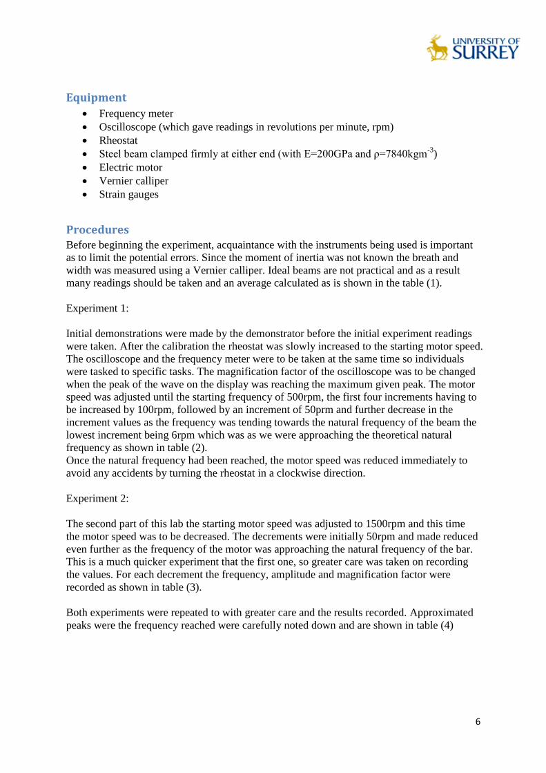
PROCEDURES AND EQUIPMENT:

Figure 3a: Steel beam supporting the electric motor

3b: Oscilloscope measuring the amplitude of vibration from strain gauges

6

Equipment

Frequency meter

Oscilloscope (which gave readings in revolutions per minute, rpm)

Rheostat

Steel beam clamped firmly at either end (with E=200GPa and ρ=7840kgm-3

)

Electric motor

Vernier calliper

Strain gauges

Procedures Before beginning the experiment, acquaintance with the instruments being used is important

as to limit the potential errors. Since the moment of inertia was not known the breath and

width was measured using a Vernier calliper. Ideal beams are not practical and as a result

many readings should be taken and an average calculated as is shown in the table (1).

Experiment 1:

Initial demonstrations were made by the demonstrator before the initial experiment readings

were taken. After the calibration the rheostat was slowly increased to the starting motor speed.

The oscilloscope and the frequency meter were to be taken at the same time so individuals

were tasked to specific tasks. The magnification factor of the oscilloscope was to be changed

when the peak of the wave on the display was reaching the maximum given peak. The motor

speed was adjusted until the starting frequency of 500rpm, the first four increments having to

be increased by 100rpm, followed by an increment of 50prm and further decrease in the

increment values as the frequency was tending towards the natural frequency of the beam the

lowest increment being 6rpm which was as we were approaching the theoretical natural

frequency as shown in table (2).

Once the natural frequency had been reached, the motor speed was reduced immediately to

avoid any accidents by turning the rheostat in a clockwise direction.

Experiment 2:

The second part of this lab the starting motor speed was adjusted to 1500rpm and this time

the motor speed was to be decreased. The decrements were initially 50rpm and made reduced

even further as the frequency of the motor was approaching the natural frequency of the bar.

This is a much quicker experiment that the first one, so greater care was taken on recording

the values. For each decrement the frequency, amplitude and magnification factor were

recorded as shown in table (3).

Both experiments were repeated to with greater care and the results recorded. Approximated

peaks were the frequency reached were carefully noted down and are shown in table (4)

7

RESULTS:

Table 1: Measurements of length, width and breath of the beam

1st 2nd 3rd 4th

5th

Average

Length (L)

±0.5mm

1115 1113 1114 - - 1114

Breath (b)

±0.01mm

50.18 50.08 50.02 50.10 50.08 50.09

Width (d)

±0.01mm

12.20 12.36 12.12 12.20 12.06 12.19

To calculate the moment of inertia of the beam the width and breath are substituted into

equation (4), where the width d is the smallest quantity, this is done when calculating the

moment of inertia to save as a safety minimal limit.

( )( )

The mass of the beam can be calculated using equation (6), since the quantities of the length;

breath and width have already been recorded. Mass of the beam will allow the calculation of

the theoretical frequency.

Table 2: Frequency-amplitude of first and repeated experiment of case 1

Where the frequency (f) and amplitude (δ)

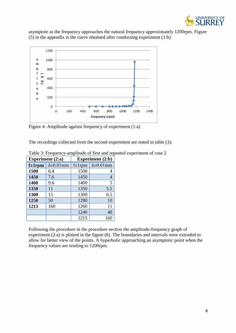
Using the information in the table (2), the amplitude against frequency of experiment (1:a) is

plotted in figure (4). The results show an asymptotic curve that approaches a point of

Experiment (1:a) Experiment (1:b)

f±1rpm δ±0.01mm f±1rpm δ±0.01mm

500 0.052 500 0.048

600 0.096 600 0.064

700 0.275 700 0.072

800 0.5 800 0.09

850 0.525 850 0.1

900 0.55 900 0.3

950 1.3 950 0.45

1000 2 1000 0.65

1030 2.4 1050 1.4

1060 2.8 1100 2.4

1090 8.8 1125 3.1

1120 13 1135 5

1150 51 1145 12

1160 130 1155 18

1165 210 1165 22

1170 440 1175 100

1176 960 1184 400

8

asymptote as the frequency approaches the natural frequency approximately 1200rpm. Figure

(5) in the appendix is the curve obtained after conducting experiment (1:b).

Figure 4: Amplitude against frequency of experiment (1:a)

The recordings collected from the second experiment are noted in table (3):

Table 3: Frequency-amplitude of first and repeated experiment of case 2

Experiment (2:a) Experiment (2:b)

f±1rpm δ±0.01mm f±1rpm δ±0.01mm

1500 6.4 1500 4

1450 7.6 1450 4

1400 9.6 1400 5

1350 11 1350 5.5

1300 15 1300 6.5

1250 50 1280 10

1213 160 1260 11

1240 48

1215 160

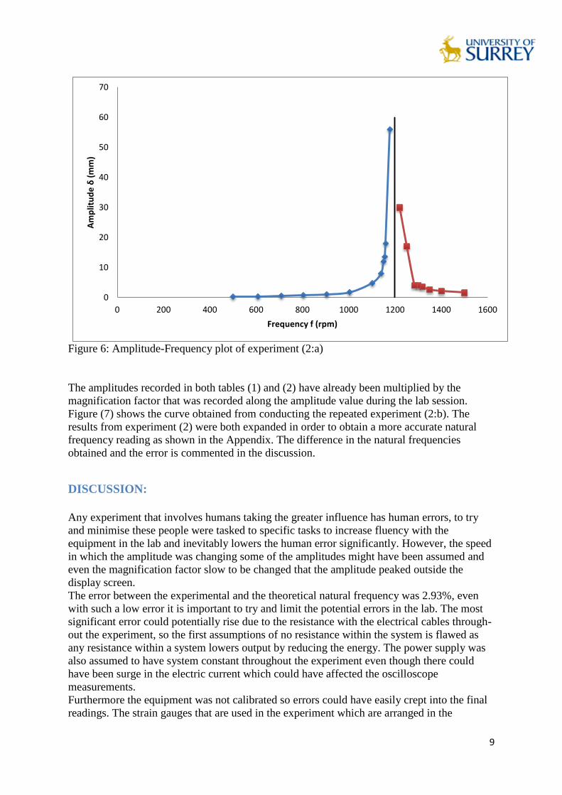
Following the procedure in the procedure section the amplitude-frequency graph of

experiment (2:a) is plotted in the figure (6). The boundaries and intervals were extruded to

allow for better view of the points. A hyperbolic approaching an asymptotic point when the

frequency values are tending to 1200rpm.

9

Figure 6: Amplitude-Frequency plot of experiment (2:a)

The amplitudes recorded in both tables (1) and (2) have already been multiplied by the

magnification factor that was recorded along the amplitude value during the lab session.

Figure (7) shows the curve obtained from conducting the repeated experiment (2:b). The

results from experiment (2) were both expanded in order to obtain a more accurate natural

frequency reading as shown in the Appendix. The difference in the natural frequencies

obtained and the error is commented in the discussion.

DISCUSSION:

Any experiment that involves humans taking the greater influence has human errors, to try

and minimise these people were tasked to specific tasks to increase fluency with the

equipment in the lab and inevitably lowers the human error significantly. However, the speed

in which the amplitude was changing some of the amplitudes might have been assumed and

even the magnification factor slow to be changed that the amplitude peaked outside the

display screen.

The error between the experimental and the theoretical natural frequency was 2.93%, even

with such a low error it is important to try and limit the potential errors in the lab. The most

significant error could potentially rise due to the resistance with the electrical cables through-

out the experiment, so the first assumptions of no resistance within the system is flawed as

any resistance within a system lowers output by reducing the energy. The power supply was

also assumed to have system constant throughout the experiment even though there could

have been surge in the electric current which could have affected the oscilloscope

measurements.

Furthermore the equipment was not calibrated so errors could have easily crept into the final

readings. The strain gauges that are used in the experiment which are arranged in the

0

10

20

30

40

50

60

70

0 200 400 600 800 1000 1200 1400 1600

Am

plit

ud

e δ

(m

m)

Frequency f (rpm)

10

Wheatstone bridge arrangement can measure different values in all of the resistors and

providing an error in the readings that are obtained. The temperature on the day rose steadily

and temperature can have a big effect on the material properties changing the ways in which

the atomic structures work due to excitement hence altering usual behaviours interestingly the

experiment considered that the temperature does not change and no reading were made

throughout the experiment. External forces vibrations were not considered this might have

had an additional effect to the external force.

The theoretical Young’s Modulus of the beam was not calculated and this can greatly affect

the final theoretical value also not determined was the density of the beam taking both

considerations into the theoretical calculations great differences might result in the final

theoretical value.

All the equipment in the experiment should be calibrated before the start of the experiment to

help obtain accurate values of and minimise the calibration error. A set power source that

supplies a steady current can also be used to eliminate the potential surge in the electric

current from the national grid. A computer can automatically receive the results and

simultaneously plotted, this would eliminate the human error caused by the delay.

Although there are many potential sources of errors as mentioned above, a low total

percentage error of 2.93% shows that the experiment is good way of finding the natural

frequency. This experiment is a very good way of finding the natural frequency and

improvement of the equipment can result in further reduction of the errors.

CONCLUSION:

The experiment was successful in obtaining the natural frequency of the beam with great

accuracy. Different beams with different Young’s modulus and lengths should be used to

validate the accuracy of our method. Also recording the room temperature before, during and

after the experiment should help improve the experiment. Ways of reducing the potential

errors in the lab have been discussed in the discussion section. The discussion section

outlines ways in which better results can be obtained.

11

REFERENCES:

[1] Rao S.S., 1990, Mechanical vibrations, Second Edition, Addison Wesley

[2] Steidel R.F Jr., 1979, An Introduction to Mechanical vibrations, Second Edition, John

Wiley and sons

[3] Thomson W.T., 1988, Theory of Vibration, Third Edition, Allen & Unwin

[4] Wahab M.A., 2008, Dynamics and Vibrations, An introduction, Revised First Edition,

John Wiley and sons

[5] Henslee. E. and Ward. S., 2013. Numerical and Experimental Methods: Background

Documents and Methods. University of Surrey

[6] Iverson C.. (11/01/11). Harmonically Driver Oscillators and Resonance. Available:

http://www.civerson.com/M275/pages/37.html. Last accessed 10th May 2015.

12

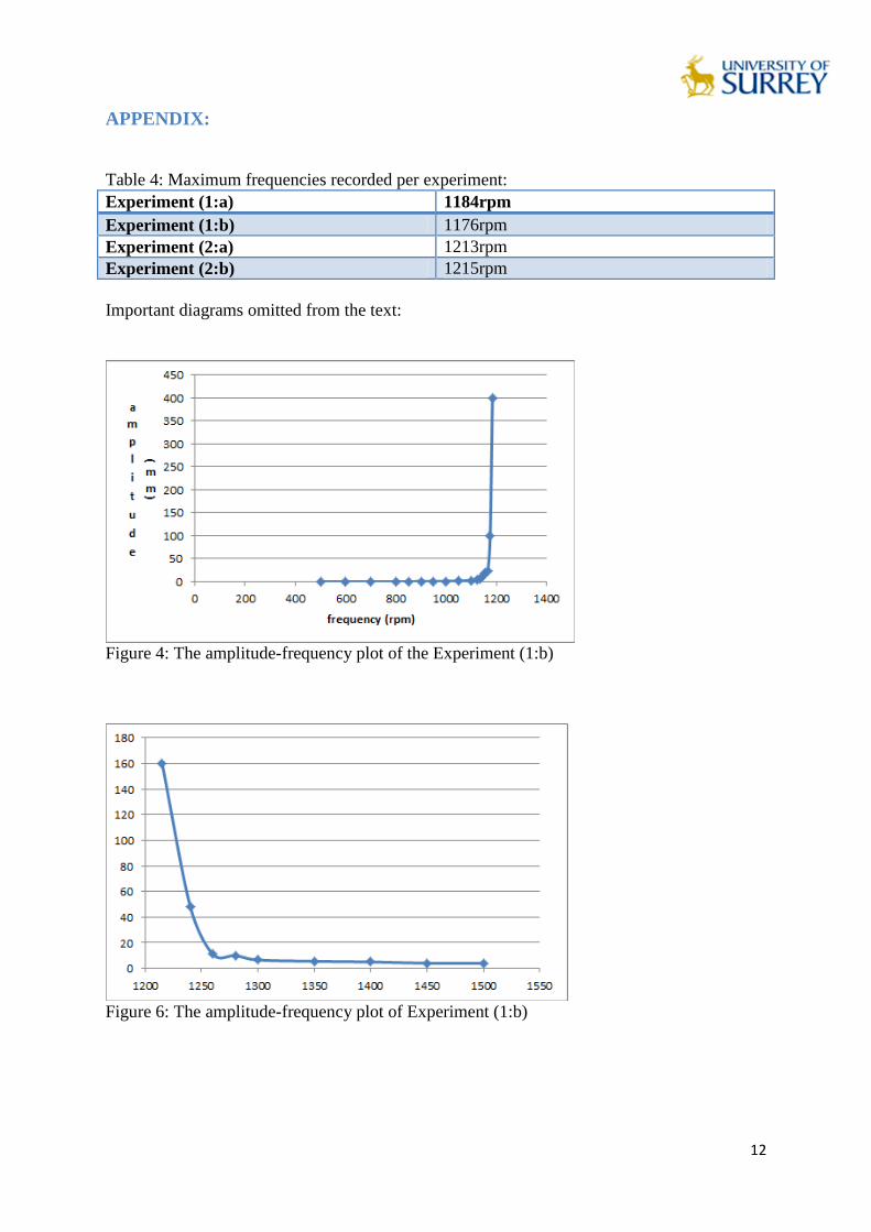
APPENDIX:

Table 4: Maximum frequencies recorded per experiment:

Experiment (1:a) 1184rpm

Experiment (1:b) 1176rpm

Experiment (2:a) 1213rpm

Experiment (2:b) 1215rpm

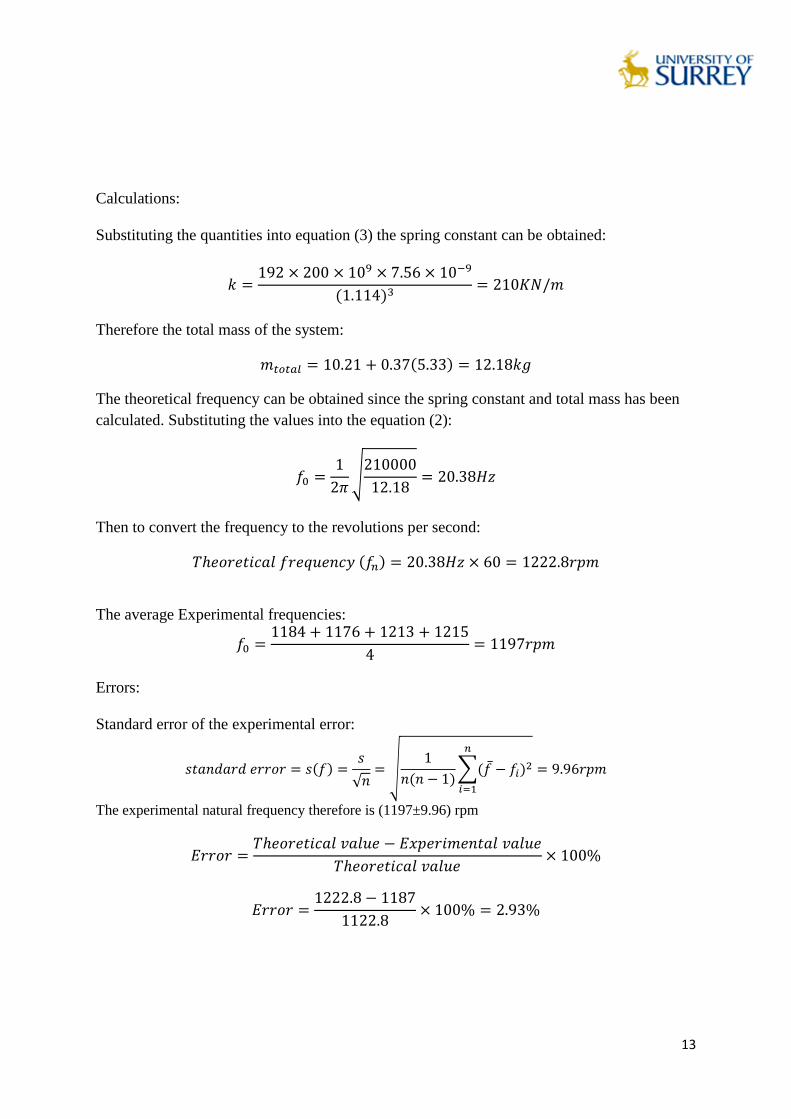
Important diagrams omitted from the text:

Figure 4: The amplitude-frequency plot of the Experiment (1:b)

Figure 6: The amplitude-frequency plot of Experiment (1:b)

13

Calculations:

Substituting the quantities into equation (3) the spring constant can be obtained:

( )

Therefore the total mass of the system:

( )

The theoretical frequency can be obtained since the spring constant and total mass has been

calculated. Substituting the values into the equation (2):

√

Then to convert the frequency to the revolutions per second:

( )

The average Experimental frequencies:

Errors:

Standard error of the experimental error:

( )

√ √

( )∑( ̅ )

The experimental natural frequency therefore is (1197±9.96) rpm