Embed Size (px)
Citation preview
Forced Vibrations
After studying the case of the free vibration, let us turn our attention to forced vibration. We will just study the mass-spring system, which is governed by the equation
𝑚𝑦′′ 𝑡 + 𝛾𝑦′ 𝑡 + 𝑘𝑦 𝑡 = 𝐹(𝑡) A simple case of forced vibration is a vertical mass-spring system that is subject to gravity.
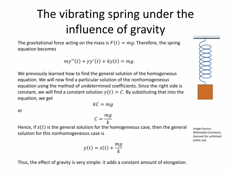
The vibrating spring under the influence of gravity
The gravitational force acting on the mass is 𝐹 𝑡 = 𝑚𝑚. Therefore, the spring equation becomes 𝑚𝑦′′ 𝑡 + 𝛾𝑦′ 𝑡 + 𝑘𝑦 𝑡 = 𝑚𝑚. We previously learned how to find the general solution of the homogeneous equation. We will now find a particular solution of the nonhomogeneous equation using the method of undetermined coefficients. Since the right side is constant, we will find a constant solution 𝑦 𝑡 = 𝐶. By substituting that into the equation, we get
𝑘𝐶 = 𝑚𝑚 or
𝐶 =𝑚𝑚𝑘
Hence, if z 𝑡 is the general solution for the homogeneous case, then the general solution for this nonhomogeneous case is
𝑦 𝑡 = 𝑧 𝑡 +𝑚𝑚𝑘
Thus, the effect of gravity is very simple: it adds a constant amount of elongation.
Image Source: Wikimedia Commons, licensed for unlimited public use.
Periodic forcing functions
We will now study a more difficult case, that of a periodic forcing function. This case is of great physical interest because mechanical and electric oscillators are often subject to periodic external forces. A circuit for example may be attached to an AC power source, or be exposed to radio waves. A mass-spring system like the shock absorbers in your car can be subject to periodic external forces as you drive on certain roads.
A general analysis of forced vibration with a periodic forcing term
Let us assume that the 𝐹(𝑡) in
𝑚𝑦′′ 𝑡 + 𝛾𝑦′ 𝑡 + 𝑘𝑦 𝑡 = 𝐹(𝑡) is periodic with frequency 𝜔 > 0 and of the form
𝐹 𝑡 = 𝐹0 cos𝜔𝑡 with a constant 𝐹0 > 0. We will try to find a particular solution y 𝑡 by using the method of undetermined coefficients:
y 𝑡 = 𝐴 cos𝜔𝑡 + 𝐵 sin𝜔𝑡
By substituting the assumed form of the solution into the differential equation, we get
𝑚𝜔2 −𝐴 cos𝜔𝑡 − 𝐵 sin𝜔𝑡 + 𝛾𝜔 −𝐴 sin𝜔𝑡 + 𝐵 cos𝜔𝑡+ 𝑘 𝐴 cos𝜔𝑡 + 𝐵 sin𝜔𝑡 = 𝐹0 cos𝜔𝑡
We simplify by combining cos and sin terms: cos𝜔𝑡 −m𝜔2A + 𝛾𝜔𝐵 + 𝑘𝐴 + sin𝜔𝑡 −𝑚𝜔2𝐵 − 𝛾𝜔𝐴 + 𝑘𝐵 = 𝐹0 cos𝜔𝑡 which leads to cos𝜔𝑡 𝛾𝜔𝐵 + (𝑘 −𝑚𝜔2)𝐴 + sin𝜔𝑡 −𝛾𝜔𝐴 + (𝑘 −𝑚𝜔2)𝐵 = 𝐹0 cos𝜔𝑡 In order for the two sides to be equal, we require
𝑘 −𝑚𝜔2 𝐴 + 𝛾𝜔𝐵 = 𝐹0
−𝛾𝜔𝐴 + 𝑘 −𝑚𝜔2 𝐵 = 0
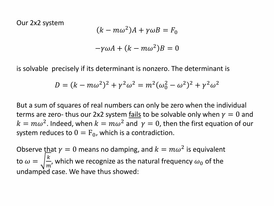
Our 2x2 system 𝑘 −𝑚𝜔2 𝐴 + 𝛾𝜔𝐵 = 𝐹0
−𝛾𝜔𝐴 + 𝑘 −𝑚𝜔2 𝐵 = 0
is solvable precisely if its determinant is nonzero. The determinant is
𝐷 = 𝑘 −𝑚𝜔2 2 + 𝛾2𝜔2 = 𝑚2 𝜔02 − 𝜔2 2 + 𝛾2𝜔2 But a sum of squares of real numbers can only be zero when the individual terms are zero- thus our 2x2 system fails to be solvable only when 𝛾 = 0 and 𝑘 = 𝑚𝜔2. Indeed, when 𝑘 = 𝑚𝜔2 and 𝛾 = 0, then the first equation of our system reduces to 0 = F0, which is a contradiction. Observe that 𝛾 = 0 means no damping, and 𝑘 = 𝑚𝜔2 is equivalent to 𝜔 = 𝑘
𝑚, which we recognize as the natural frequency 𝜔0 of the
undamped case. We have thus showed:
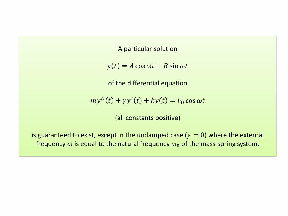
A particular solution
y 𝑡 = 𝐴 cos𝜔𝑡 + 𝐵 sin𝜔𝑡
of the differential equation
𝑚𝑦′′ 𝑡 + 𝛾𝑦′ 𝑡 + 𝑘𝑦 𝑡 = 𝐹0 cos𝜔𝑡
(all constants positive)
is guaranteed to exist, except in the undamped case (𝛾 = 0) where the external frequency 𝜔 is equal to the natural frequency 𝜔0 of the mass-spring system.
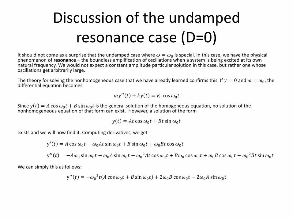
Discussion of the undamped resonance case (D=0)
It should not come as a surprise that the undamped case where 𝜔 = 𝜔0 is special. In this case, we have the physical phenomenon of resonance – the boundless amplification of oscillations when a system is being excited at its own natural frequency. We would not expect a constant amplitude particular solution in this case, but rather one whose oscillations get arbitrarily large. The theory for solving the nonhomogeneous case that we have already learned confirms this. If 𝛾 = 0 and 𝜔 = 𝜔0, the differential equation becomes
𝑚𝑦′′ 𝑡 + 𝑘𝑦 𝑡 = 𝐹0 cos𝜔0𝑡 Since y 𝑡 = 𝐴 cos𝜔0𝑡 + 𝐵 sin𝜔0𝑡 is the general solution of the homogeneous equation, no solution of the nonhomogeneous equation of that form can exist. However, a solution of the form
y 𝑡 = 𝐴𝑡 cos𝜔0𝑡 + 𝐵𝑡 sin𝜔0𝑡 exists and we will now find it. Computing derivatives, we get y′ 𝑡 = 𝐴 cos𝜔0𝑡 − 𝜔0𝐴𝑡 sin𝜔0𝑡 +𝐵 sin𝜔0𝑡 + 𝜔0𝐵𝑡 cos𝜔0𝑡 y′′ 𝑡 = −𝐴𝜔0 sin𝜔0𝑡 − 𝜔0𝐴 sin𝜔0𝑡 − 𝜔02𝐴𝑡 cos𝜔0𝑡 + 𝐵𝜔0 cos𝜔0𝑡 + 𝜔0𝐵 cos𝜔0𝑡 − 𝜔02𝐵𝑡 sin𝜔0𝑡 We can simply this as follows:
y′′ 𝑡 = −𝜔02𝑡 𝐴 cos𝜔0𝑡 + 𝐵 sin𝜔0𝑡 + 2𝜔0𝐵 cos𝜔0𝑡 − 2𝜔0𝐴 sin𝜔0𝑡
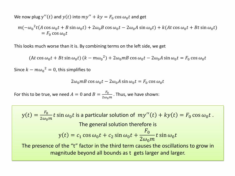
We now plug y′′ 𝑡 and 𝑦 𝑡 into 𝑚𝑦′′ + 𝑘𝑦 = 𝐹0 cos𝜔0𝑡 and get 𝑚(−𝜔0
2𝑡 𝐴 cos𝜔0𝑡 + 𝐵 sin𝜔0𝑡 + 2𝜔0𝐵 cos𝜔0𝑡 − 2𝜔0𝐴 sin𝜔0𝑡) + 𝑘(𝐴𝑡 cos𝜔0𝑡 + 𝐵𝑡 sin𝜔0𝑡)= 𝐹0 cos𝜔0𝑡
This looks much worse than it is. By combining terms on the left side, we get
(A𝑡 cos𝜔0𝑡 + 𝐵𝑡 sin𝜔0𝑡) (𝑘 − 𝑚𝜔02) + 2𝜔0𝑚𝐵 cos𝜔0𝑡 − 2𝜔0𝐴 sin𝜔0𝑡 = 𝐹0 cos𝜔0𝑡
Since 𝑘 − 𝑚𝜔0
2 = 0, this simplifies to
2𝜔0𝑚𝐵 cos𝜔0𝑡 − 2𝜔0𝐴 sin𝜔0𝑡 = 𝐹0 cos𝜔0𝑡 For this to be true, we need 𝐴 = 0 and 𝐵 = 𝐹0
2𝜔0𝑚 . Thus, we have shown:
y 𝑡 = 𝐹02𝜔0𝑚
𝑡 sin𝜔0𝑡 is a particular solution of 𝑚𝑦′′ 𝑡 + 𝑘𝑦 𝑡 = 𝐹0 cos𝜔0𝑡 . The general solution therefore is
y 𝑡 = 𝑐1 cos𝜔0𝑡 + 𝑐2 sin𝜔0𝑡 +𝐹0
2𝜔0𝑚𝑡 sin𝜔0𝑡
The presence of the “t” factor in the third term causes the oscillations to grow in magnitude beyond all bounds as t gets larger and larger.
Having successfully explored the special case where 𝐷 = 𝑘 − 𝑚𝜔2 2 + 𝛾2𝜔2 = 0, we now turn our attention to the case where 𝐷 > 0. Recall that in that case, a particular solution of the form y 𝑡 = 𝐴 cos𝜔𝑡 + 𝐵 sin𝜔𝑡 exists for the equation
𝑚𝑦′′ 𝑡 + 𝛾𝑦′ 𝑡 + 𝑘𝑦 𝑡 = 𝐹0 cos𝜔𝑡 and the coefficients A,B must satisfy
𝑘 − 𝑚𝜔2 𝐴 + 𝛾𝜔𝐵 = 𝐹0
−𝛾𝜔𝐴 + 𝑘 − 𝑚𝜔2 𝐵 = 0 Since the determinant 𝐷 is now assumed to be nonzero, we can use Cramer’s rule to solve for A and B:
𝐴 =𝐹0 𝑘 − 𝑚𝜔2
𝐷 =𝐹0𝑚 𝜔02 − 𝜔2
𝐷
B =𝐹0𝛾𝜔𝐷
We have thus found a particular solution of
𝑚𝑦′′ 𝑡 + 𝛾𝑦′ 𝑡 + 𝑘𝑦 𝑡 = 𝐹0 cos𝜔𝑡 for the case 𝐷 > 0:
y 𝑡 =𝐹0𝑚 𝜔02 − 𝜔2
𝐷 cos𝜔𝑡 +𝐹0𝛾𝜔𝐷
sin𝜔𝑡 Recall from a previous presentation that 𝑐1 cos𝜇𝑡 + 𝑐2 sin 𝜇𝑡 can be rewritten as a single, phase-shifted sine (or cosine) wave with amplitude
A = 𝑐12 + 𝑐22 It follows that the amplitude of our particular solution is
A =𝐹0𝐷 𝑚2 𝜔02 − 𝜔2 2 + 𝛾2𝜔2 =
𝐹0𝐷
Having found a particular solution, we turn our attention to the general solution. If 𝑦ℎ 𝑡 is the general solution of the homogeneous equation, then the general solution of the nonhomogeneous case is
y 𝑡 = 𝑦ℎ 𝑡 +𝐹0𝑚 𝜔02 − 𝜔2
𝐷 cos𝜔𝑡 +𝐹0𝛾𝜔𝐷 sin𝜔𝑡
Discussion of the case D>0 Recall that the determinant is 𝐷 = 𝑚2 𝜔02 − 𝜔2 2 + 𝛾2𝜔2. We will discuss the damped and the undamped situations separately. First let us discuss the damped case 𝛾 > 0. In that case, 𝐷 > 0 even when ω = 𝜔0. The general solution we found is
y 𝑡 = 𝑦ℎ 𝑡 +𝐹0𝑚 𝜔02 − 𝜔2
𝐷cos𝜔𝑡 +
𝐹0𝛾𝜔𝐷
sin𝜔𝑡particular solution
Let us simplify the notation by calling the particular solution 𝑦𝑝 𝑡 :
y 𝑡 = 𝑦ℎ 𝑡 + 𝑦𝑝 𝑡 Recall from a previous presentation that in the damped case, all solutions of the homogeneous equation decay exponentially. This means that over time, as 𝑡 → ∞, the term 𝑦ℎ 𝑡 goes to zero, and only the particular solution 𝑦𝑝 𝑡 remains.
This is why 𝑦ℎ 𝑡 is called the transient solution, whereas 𝑦𝑝 𝑡 is called the steady state solution or forced response. Over time, ALL solutions, regardless of the initial conditions, “settle into” (become approximately equal to ) the steady state solution. This is important because the transient solution 𝑦ℎ 𝑡 contains the information about the initial conditions whereas the steady state solution 𝑦𝑝 𝑡 does not. The damped, forced system “forgets” its initial condition over time. A physical interpretation of this phenomenon is that damping dissipates the energy embodied in the initial position and velocity, and that the long-term behavior of the system is solely determined by the external periodic force.
The damped case with D>0
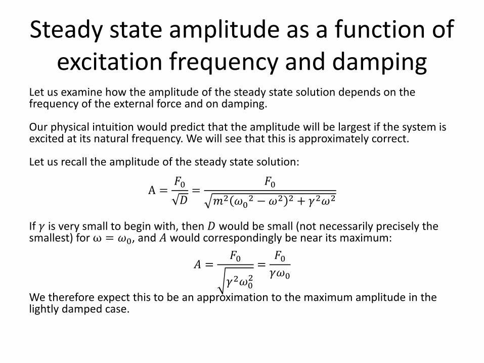
Steady state amplitude as a function of excitation frequency and damping
Let us examine how the amplitude of the steady state solution depends on the frequency of the external force and on damping. Our physical intuition would predict that the amplitude will be largest if the system is excited at its natural frequency. We will see that this is approximately correct. Let us recall the amplitude of the steady state solution:
A =𝐹0𝐷
=𝐹0
𝑚2 𝜔02 − 𝜔2 2 + 𝛾2𝜔2
If 𝛾 is very small to begin with, then 𝐷 would be small (not necessarily precisely the smallest) for ω = 𝜔0, and 𝐴 would correspondingly be near its maximum:
𝐴 =𝐹0
𝛾2𝜔02=
𝐹0𝛾𝜔0
We therefore expect this to be an approximation to the maximum amplitude in the lightly damped case.
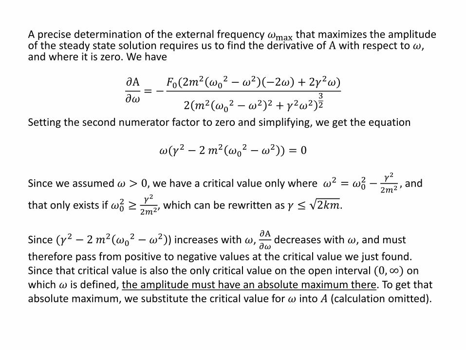
A precise determination of the external frequency 𝜔max that maximizes the amplitude of the steady state solution requires us to find the derivative of A with respect to 𝜔, and where it is zero. We have
𝜕A𝜕𝜔 = −
𝐹0(2𝑚2 𝜔02 − 𝜔2 −2𝜔 + 2𝛾2𝜔)
2 𝑚2 𝜔02 − 𝜔2 2 + 𝛾2𝜔232
Setting the second numerator factor to zero and simplifying, we get the equation
𝜔(𝛾2 − 2 𝑚2 𝜔02 − 𝜔2 ) = 0
Since we assumed 𝜔 > 0, we have a critical value only where 𝜔2 = 𝜔02 −𝛾2
2𝑚2 , and
that only exists if 𝜔02 ≥𝛾2
2𝑚2, which can be rewritten as 𝛾 ≤ 2𝑘𝑚. Since (𝛾2 − 2 𝑚2 𝜔02 − 𝜔2 ) increases with 𝜔, 𝜕A
𝜕𝜔 decreases with 𝜔, and must
therefore pass from positive to negative values at the critical value we just found. Since that critical value is also the only critical value on the open interval (0,∞) on which 𝜔 is defined, the amplitude must have an absolute maximum there. To get that absolute maximum, we substitute the critical value for 𝜔 into 𝐴 (calculation omitted).
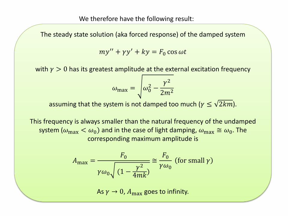
We therefore have the following result:
The steady state solution (aka forced response) of the damped system
𝑚𝑦′′ + 𝛾𝑦′ + 𝑘𝑦 = 𝐹0 cos𝜔𝑡
with 𝛾 > 0 has its greatest amplitude at the external excitation frequency
𝜔max = 𝜔02 −𝛾2
2𝑚2
assuming that the system is not damped too much (𝛾 ≤ 2𝑘𝑚).
This frequency is always smaller than the natural frequency of the undamped system (𝜔max < 𝜔0) and in the case of light damping, 𝜔max ≅ 𝜔0. The
corresponding maximum amplitude is
𝐴max =𝐹0
𝛾𝜔0 (1 − 𝛾24𝑚𝑘)
≅𝐹0𝛾𝜔0
for small 𝛾
As 𝛾 → 0, 𝐴max goes to infinity.
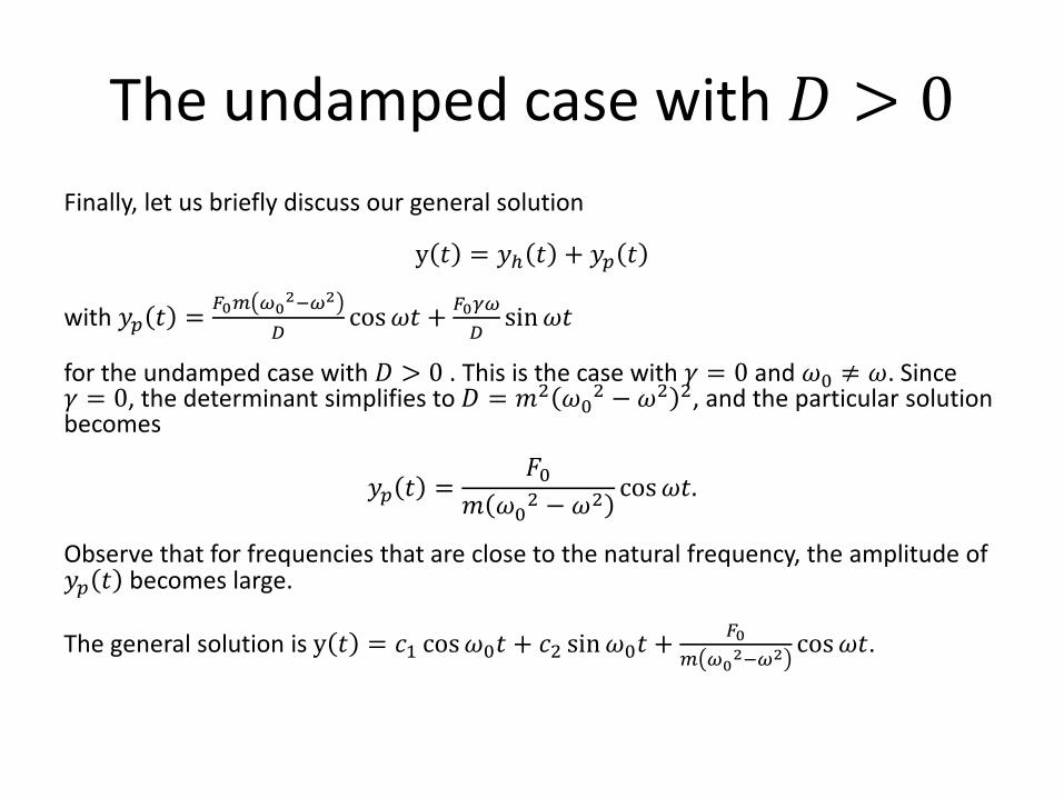
The undamped case with 𝐷 > 0 Finally, let us briefly discuss our general solution
y 𝑡 = 𝑦ℎ 𝑡 + 𝑦𝑝 𝑡 with 𝑦𝑝 𝑡 = 𝐹0𝑚 𝜔0
2−𝜔2
𝐷cos𝜔𝑡 + 𝐹0𝛾𝜔
𝐷sin𝜔𝑡
for the undamped case with 𝐷 > 0 . This is the case with 𝛾 = 0 and 𝜔0 ≠ 𝜔. Since 𝛾 = 0, the determinant simplifies to 𝐷 = 𝑚2 𝜔02 − 𝜔2 2, and the particular solution becomes
𝑦𝑝 𝑡 =𝐹0
𝑚 𝜔02 − 𝜔2 cos𝜔𝑡. Observe that for frequencies that are close to the natural frequency, the amplitude of 𝑦𝑝 𝑡 becomes large. The general solution is y 𝑡 = 𝑐1 cos𝜔0𝑡 + 𝑐2 sin𝜔0𝑡 + 𝐹0
𝑚 𝜔02−𝜔2 cos𝜔𝑡.
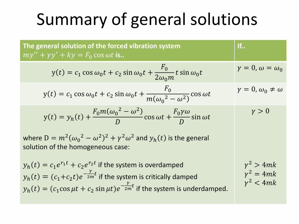
Summary of general solutions The general solution of the forced vibration system 𝑚𝑦′′ + 𝛾𝑦′ + 𝑘𝑦 = 𝐹0 cos𝜔𝑡 is..
If..
y 𝑡 = 𝑐1 cos𝜔0𝑡 + 𝑐2 sin𝜔0𝑡 +𝐹0
2𝜔0𝑚𝑡 sin𝜔0𝑡
𝛾 = 0, 𝜔 = 𝜔0
y 𝑡 = 𝑐1 cos𝜔0𝑡 + 𝑐2 sin𝜔0𝑡 +𝐹0
𝑚 𝜔02 − 𝜔2 cos𝜔𝑡 𝛾 = 0, 𝜔0 ≠ 𝜔
y 𝑡 = 𝑦ℎ 𝑡 +𝐹0𝑚 𝜔02 − 𝜔2
𝐷 cos𝜔𝑡 +𝐹0𝛾𝜔𝐷 sin𝜔𝑡
where D = 𝑚2 𝜔02 − 𝜔2 2 + 𝛾2𝜔2 and 𝑦ℎ 𝑡 is the general solution of the homogeneous case: 𝑦ℎ 𝑡 = 𝑐1𝑒𝑟1𝑡 + 𝑐2𝑒𝑟2𝑡 if the system is overdamped
𝑦ℎ 𝑡 = (𝑐1+𝑐2𝑡)𝑒− 𝛾2𝑚𝑡 if the system is critically damped
𝑦ℎ 𝑡 = (𝑐1cos𝜇𝑡 + 𝑐2 sin𝜇𝑡)𝑒−𝛾2𝑚𝑡 if the system is underdamped.
𝛾 > 0 𝛾2 > 4𝑚𝑘 𝛾2 = 4𝑚𝑘 𝛾2 < 4𝑚𝑘


![M P Jump3R - Everyone Forgets the Beginning [Completed]](https://img.pdfslide.net/doc/110x75/577cc6b91a28aba7119ef8b8/m-p-jump3r-everyone-forgets-the-beginning-completed.jpg)