Forcing a Distributed Glacier Mass Balance Model with the

Forcing a Distributed Glacier Mass Balance Model with the Regional ClimateModel REMO. Part I: Climate Model Evaluation

SVEN KOTLARSKI*

Max Planck Institute for Meteorology, Hamburg, Germany

FRANK PAUL

Department of Geography, University of Zurich, Zurich, Switzerland

DANIELA JACOB

Max Planck Institute for Meteorology, Hamburg, Germany

(Manuscript received 7 July 2008, in final form 13 July 2009)

ABSTRACT

A coupling interface between the regional climate model REMO and a distributed glacier mass balance

model is presented in a series of two papers. The first part describes and evaluates the reanalysis-driven

regional climate simulation that is used to force a mass balance model for two glaciers of the Swiss mass

balance network. The detailed validation of near-surface air temperature, precipitation, and global radiation

for the European Alps shows that the basic spatial and temporal patterns of all three parameters are

reproduced by REMO. Compared to the Climatic Research Unit (CRU) dataset, the Alpine mean tem-

perature is underestimated by 0.348C. Annual precipitation shows a positive bias of 17% (30%) with respect

to the uncorrected gridded ALP-IMP (CRU) dataset. A number of important and systematic model biases

arise in high-elevation regions, namely, a negative temperature bias in winter, a bias of seasonal precipitation

(positive or negative, depending on gridbox altitude and season), and an underestimation of springtime and

overestimation of summertime global radiation. These can be expected to have a strong effect on the sim-

ulated glacier mass balance. It is recommended to account for these shortcomings by applying correction

procedures before using the RCM output for subsequent mass balance modeling. Despite the obvious model

deficiencies in high-elevation regions, the new interface broadens the scope of application of glacier mass

balance models and will allow for a straightforward assessment of future climate change impacts.

1. Introduction

During the past 100 years mountain regions all around

the globe experienced considerable glacier mass losses

and large reductions in glacier area (WGMS 2008). The

European Alps, for instance, had lost about 50% of their

1850s ice mass by the 1980s (Haeberli and Hoelzle 1995)

and melt rates even accelerated toward the end of the

twentieth century (Paul et al. 2004; Zemp et al. 2008).

Such variations in glacier mass are determined by the

balance between incoming (mass gain) and outgoing (mass

loss) terms and the underlying processes are strongly

controlled by atmospheric factors.

To assess the response of a glacier’s mass balance to

changing atmospheric conditions, spatially distributed

mass balance models (MBMs) were applied in numer-

ous studies (e.g., Arnold et al. 1996; Hock 1999; Brock

et al. 2000; Klok and Oerlemans 2002; Machguth et al.

2006). Depending on their complexity, these models

incorporate a number of meteorological input parame-

ters and simulate the temporal evolution of mass bal-

ance terms (accumulation and ablation) in the course of

a year or over several years (Oerlemans 2001). The at-

mospheric forcing is usually provided by weather station

data near to or on the glacier surface, which are in-

terpolated to the required horizontal resolution of the

* Current affiliation: Institute for Atmospheric and Climate

Science, ETH Zurich, Zurich, Switzerland.

Corresponding author address: Sven Kotlarski, Institute for At-

mospheric and Climate Science, ETH Zurich, Universitaetstrasse

16, CH-8092 Zurich, Switzerland.

E-mail: [email protected]

15 MARCH 2010 K O T L A R S K I E T A L . 1589

DOI: 10.1175/2009JCLI2711.1

� 2010 American Meteorological Society

MBM. In most studies, only individual glaciers are

considered (e.g., Stahl et al. 2008). The step to larger re-

gions covering major river catchments or entire mountain

ranges has only seldom been made, although distributed

energy balance models are well suited for such large-

scale applications. This can partly be explained by the

fact that the application of an MBM to a large number

of individual glaciers simultaneously requires both in-

formation on glacier characteristics [i.e., extent and a

digital elevation model (DEM)] and atmospheric forc-

ing datasets with a high spatial resolution for a large

domain. In regions with good data coverage the latter

can often be provided by interpolated station data. This

is true for temperature and precipitation in the Euro-

pean Alps toward the end of the twentieth century.

However, the data coverage is sparser in most other

mountain regions, for other parameters than tempera-

ture and precipitation (e.g., global radiation) and for

periods before the 1970s. For this reason, global appli-

cations like the assessment of the contribution of glacier

melt to future sea level rise still apply a simplifying

degree-day approach (e.g., Van de Wal and Wild 2001;

Raper and Braithwaite 2006).

Instead of using interpolated station data as atmo-

spheric forcing, an increasingly interesting option for the

large-scale application of MBMs is to drive them with

output of regional climate models (RCMs). In recent

years, these models proved to be useful tools for the

analysis of regional energy and water cycles as well as for

the projection of climatic changes on a regional scale (e.g.,

Jacob et al. 2001; Kotlarski et al. 2005; Deque et al. 2005;

Jacob et al. 2007; Christensen and Christensen 2007).

Similarly to general circulation models (GCMs), RCMs

account for the most relevant processes, interactions and

feedbacks between climate system components in a phys-

ically consistent manner, producing a comprehensive set

of output data at a high horizontal resolution. In moun-

tainous terrain the latter is important in order to resolve

small-scale atmospheric circulations (e.g., those affected

by orographic details of the land surface; Giorgi 1990;

McGregor 1997). If driven by reanalysis or analysis data

at the lateral boundaries (i.e., observation-based prod-

ucts describing the large-scale state of the atmosphere)

RCMs are able to approximately reproduce observed

spatial and temporal climatic patterns (e.g., Frei et al.

2003; Semmler and Jacob 2004; Kotlarski et al. 2005).

Still, systematic errors and uncertainties of RCM data

have to be considered for certain parameters (e.g., for

precipitation in Alpine regions; Frei et al. 2003). Re-

garding the coupling to mass balance models a further

point is the apparent scale gap. The currently available

spatial resolution of multiyear RCM simulations (about

10–50 km) does not allow us to resolve individual gla-

ciers and is much coarser than the resolution of state-of-

the-art MBMs (10–100 m). This requires a further treat-

ment of RCM results and the definition of an appropriate

coupling interface between both models. Such an in-

terface has to account for the further downscaling of

RCM results to the target resolution of the MBM and

could optionally also correct for systematic errors in the

RCM output. Once this interface has been set up, the

effects of regional climatic changes on glacier mass bal-

ance can be assessed in a straightforward way.

The present study, consisting of two separate parts,

investigates the benefits and the limitations of forcing

a distributed glacier mass balance model with the output

of a state-of-the-art RCM. For this purpose, a test site in

the south-central part of Switzerland was chosen that

contains two glaciers of the Swiss mass balance network:

Gries Glacier and Basodino Glacier. For both glaciers

a spatially distributed MBM is applied using 1) obser-

vational meteorological data from a nearby weather

station (Robiei) and 2) the output of the regional climate

model Regional Model (REMO). The first part of our

study (this paper) presents and evaluates the RCM sim-

ulation that will be used to drive the MBM. A focus is laid

on high-elevation regions and on those parameters that

exert a primary influence on glacier mass balance and that

will later on be used to drive the MBM (temperature,

precipitation, global radiation). Specific questions that we

are trying to answer are the following: to what extent can

a state-of-the-art RCM reproduce the spatial and tem-

poral variation of parameters relevant for glacier mass

balance? Which biases do we have to expect in high-

elevation regions and what is their seasonal and altitudinal

variation? Is there a need for correcting RCM results

before feeding them into a glacier mass balance model?

The second part of the study (Paul and Kotlarski 2010,

hereafter Part II) describes the further downscaling

of the RCM data to the resolution of the MBM and

the results of the mass balance modeling, including the

comparison of the simulated glacier mass balance to

observations.

2. Data and methods

a. RCM data

Within the present study, the RCM REMO (Jacob

and Podzun 1997; Jacob 2001; Jacob et al. 2001) was

integrated for the period 1958–2002. REMO is a three-

dimensional, hydrostatic atmospheric circulation model

that is based on the numerical weather prediction model

Europa-Modell (EM; Majewski 1991) and that includes

the physical parameterization package of the general

circulation model ECHAM4 (Roeckner et al. 1996). In

the vertical, variations of the prognostic atmospheric

1590 J O U R N A L O F C L I M A T E VOLUME 23

variables are represented by a hybrid vertical coordinate

system (Simmons and Burridge 1981). For horizontal

discretization REMO uses a rotated latitude–longitude

coordinate system with standard grid spacings between

0.0888 (approximately 10 km 3 10 km) and 0.448 (ap-

proximately 50 km 3 50 km). The lateral boundary

conditions (LBCs) can either be provided by a GCM

simulation or by reanalysis or analysis products. In all

cases, the relaxation scheme according to Davies (1976)

is applied: the prognostic variables of the RCM are ad-

justed toward the large-scale forcing in a lateral sponge

zone of eight grid boxes with the LBC influence expo-

nentially decreasing toward the inner model domain.

At the lower boundary REMO is forced by the land

and sea surface characteristics (e.g., surface tempera-

ture, albedo, surface roughness length, etc.). The model

version applied within this study (REMO 5.3) uses the

so-called tile approach in which the total surface area of

an individual model grid box can consist of a land, a

water, and a sea ice fraction on a subgrid scale (expressed

in percent). So far, glaciers are not explicitly represented

in REMO’s land surface scheme. In the European Alps

their size is much smaller than the resolved scale of the

RCM. Only the polar ice sheets are explicitly accounted

for by a static, binary glacier mask that assigns ice sur-

face characteristics to certain grid boxes and that does

not change in time. The recent development of a glacier

subgrid parameterization scheme that allows for a dy-

namic fractional ice coverage can be expected to im-

prove this deficit (Kotlarski 2007).

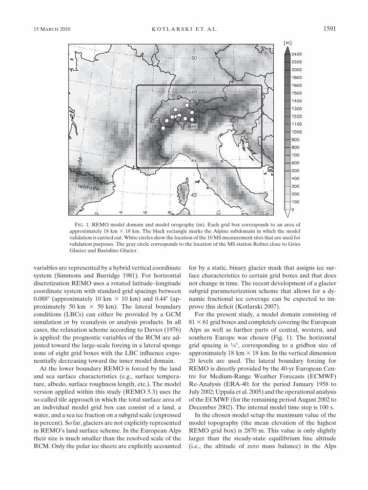
For the present study, a model domain consisting of

81 3 61 grid boxes and completely covering the European

Alps as well as further parts of central, western, and

southern Europe was chosen (Fig. 1). The horizontal

grid spacing is 1/68, corresponding to a gridbox size of

approximately 18 km 3 18 km. In the vertical dimension

20 levels are used. The lateral boundary forcing for

REMO is directly provided by the 40-yr European Cen-

tre for Medium-Range Weather Forecasts (ECMWF)

Re-Analysis (ERA-40; for the period January 1958 to

July 2002; Uppala et al. 2005) and the operational analysis

of the ECMWF (for the remaining period August 2002 to

December 2002). The internal model time step is 100 s.

In the chosen model setup the maximum value of the

model topography (the mean elevation of the highest

REMO grid box) is 2870 m. This value is only slightly

larger than the steady-state equilibrium line altitude

(i.e., the altitude of zero mass balance) in the Alps

FIG. 1. REMO model domain and model orography (m). Each grid box corresponds to an area of

approximately 18 km 3 18 km. The black rectangle marks the Alpine subdomain in which the model

validation is carried out. White circles show the location of the 10 MS measurement sites that are used for

validation purposes. The gray circle corresponds to the location of the MS station Robiei close to Gries

Glacier and Basodino Glacier.


during the last decades of the twentieth century (.2700 m

MSL in most regions; Zemp et al. 2007). This fact clearly

illustrates that, if the model results are to be used in mass

balance studies, a further downscaling of atmospheric

parameters has to be carried out in order to provide

a realistic atmospheric forcing at the site of individual

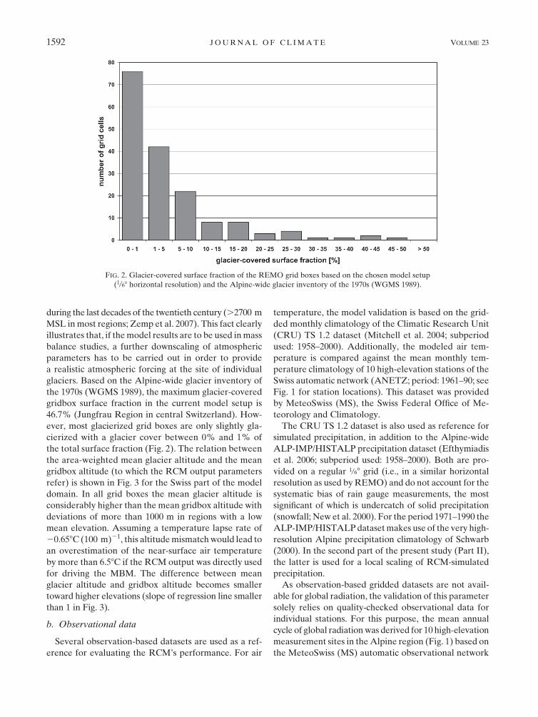
glaciers. Based on the Alpine-wide glacier inventory of

the 1970s (WGMS 1989), the maximum glacier-covered

gridbox surface fraction in the current model setup is

46.7% (Jungfrau Region in central Switzerland). How-

ever, most glacierized grid boxes are only slightly gla-

cierized with a glacier cover between 0% and 1% of

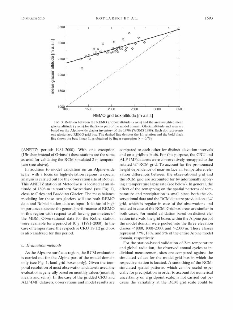
the total surface fraction (Fig. 2). The relation between

the area-weighted mean glacier altitude and the mean

gridbox altitude (to which the RCM output parameters

refer) is shown in Fig. 3 for the Swiss part of the model

domain. In all grid boxes the mean glacier altitude is

considerably higher than the mean gridbox altitude with

deviations of more than 1000 m in regions with a low

mean elevation. Assuming a temperature lapse rate of

20.658C (100 m)21, this altitude mismatch would lead to

an overestimation of the near-surface air temperature

by more than 6.58C if the RCM output was directly used

for driving the MBM. The difference between mean

glacier altitude and gridbox altitude becomes smaller

toward higher elevations (slope of regression line smaller

than 1 in Fig. 3).

b. Observational data

Several observation-based datasets are used as a ref-

erence for evaluating the RCM’s performance. For air

temperature, the model validation is based on the grid-

ded monthly climatology of the Climatic Research Unit

(CRU) TS 1.2 dataset (Mitchell et al. 2004; subperiod

used: 1958–2000). Additionally, the modeled air tem-

perature is compared against the mean monthly tem-

perature climatology of 10 high-elevation stations of the

Swiss automatic network (ANETZ; period: 1961–90; see

Fig. 1 for station locations). This dataset was provided

by MeteoSwiss (MS), the Swiss Federal Office of Me-

teorology and Climatology.

The CRU TS 1.2 dataset is also used as reference for

simulated precipitation, in addition to the Alpine-wide

ALP-IMP/HISTALP precipitation dataset (Efthymiadis

et al. 2006; subperiod used: 1958–2000). Both are pro-

vided on a regular 1/68 grid (i.e., in a similar horizontal

resolution as used by REMO) and do not account for the

systematic bias of rain gauge measurements, the most

significant of which is undercatch of solid precipitation

(snowfall; New et al. 2000). For the period 1971–1990 the

ALP-IMP/HISTALP dataset makes use of the very high-

resolution Alpine precipitation climatology of Schwarb

(2000). In the second part of the present study (Part II),

the latter is used for a local scaling of RCM-simulated

precipitation.

As observation-based gridded datasets are not avail-

able for global radiation, the validation of this parameter

solely relies on quality-checked observational data for

individual stations. For this purpose, the mean annual

cycle of global radiation was derived for 10 high-elevation

measurement sites in the Alpine region (Fig. 1) based on

the MeteoSwiss (MS) automatic observational network

FIG. 2. Glacier-covered surface fraction of the REMO grid boxes based on the chosen model setup

(1/68 horizontal resolution) and the Alpine-wide glacier inventory of the 1970s (WGMS 1989).


(ANETZ; period: 1981–2000). With one exception

(Ulrichen instead of Grimsel) these stations are the same

as used for validating the RCM-simulated 2-m tempera-

ture (see above).

In addition to model validation on an Alpine-wide

scale, with a focus on high-elevation regions, a special

analysis is carried out for the observation site of Robiei.

This ANETZ station of MeteoSwiss is located at an al-

titude of 1898 m in southern Switzerland (see Fig. 1),

close to Gries and Basodino Glacier. The mass balance

modeling for these two glaciers will use both REMO

data and Robiei station data as input. It is thus of high

importance to assess the general performance of REMO

in this region with respect to all forcing parameters of

the MBM. Observational data for the Robiei station

were available for a period of 10 yr (1991–2000). In the

case of temperature, the respective CRU TS 1.2 grid box

is also analyzed for this period.

c. Evaluation methods

As the Alps are our focus region, the RCM evaluation

is carried out for the Alpine part of the model domain

only (see Fig. 1, land grid boxes only). Given the tem-

poral resolution of most observational datasets used, the

evaluation is generally based on monthly values (monthly

means and sums). In the case of the gridded CRU and

ALP-IMP datasets, observations and model results are

compared to each other for distinct elevation intervals

and on a gridbox basis. For this purpose, the CRU and

ALP-IMP datasets were conservatively remapped to the

rotated 1/68 RCM grid. To account for the pronounced

height dependence of near-surface air temperature, ele-

vation differences between the observational grid and

the RCM grid are accounted for by additionally apply-

ing a temperature lapse rate (see below). In general, the

effect of the remapping on the spatial patterns of tem-

perature and precipitation is small since both the ob-

servational data and the RCM data are provided on a 1/68

grid, which is regular in case of the observations and

rotated in case of the RCM. Gridbox areas are similar in

both cases. For model validation based on distinct ele-

vation intervals, the grid boxes within the Alpine part of

the model domain were pooled into the three elevation

classes ,1000, 1000–2000, and .2000 m. These classes

represent 77%, 18%, and 5% of the entire Alpine model

domain, respectively.

For the station-based validation of 2-m temperature

and global radiation, the observed annual cycles at in-

dividual measurement sites are compared against the

simulated values for the model grid box in which the

respective station is located. A smoothing of the RCM-

simulated spatial patterns, which can be useful espe-

cially for precipitation in order to account for numerical

uncertainty on a gridpoint scale, is not carried out be-

cause the variability at the RCM grid scale could be

FIG. 3. Relation between the REMO gridbox altitude (x axis) and the area-weighted mean

glacier altitude (y axis) for the Swiss part of the model domain. Glacier altitude and area are

based on the Alpine-wide glacier inventory of the 1970s (WGMS 1989). Each dot represents

one glacierized REMO grid box. The dashed line denotes the 1:1 relation and the bold black

line shows the best linear fit as obtained by linear regression (r 5 0.76).


important for mass balance forcing. Furthermore, the

use of nonsmoothed fields allows for a better visibility of

shortcomings of the native RCM dataset. In the case of

2-m temperature, the elevation difference between the

RCM grid box and the measurement site is explicitly

accounted for by applying a monthly and regionally

varying temperature lapse rate to the model output. For

this purpose, monthly lapse rates for the period 1961–90

were computed for the surroundings of each individual

MeteoSwiss measurement site based on the CRU TS 1.2

temperature dataset (see above). Lapse rates were de-

rived by regressing the mean monthly temperature at

25 CRU grid boxes (square of 5 3 5 boxes with the

measurement site located in the center grid box) against

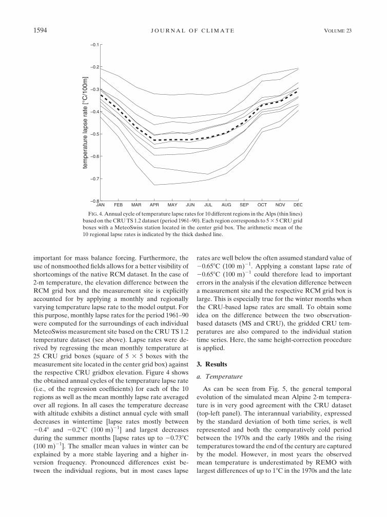
the respective CRU gridbox elevation. Figure 4 shows

the obtained annual cycles of the temperature lapse rate

(i.e., of the regression coefficients) for each of the 10

regions as well as the mean monthly lapse rate averaged

over all regions. In all cases the temperature decrease

with altitude exhibits a distinct annual cycle with small

decreases in wintertime [lapse rates mostly between

20.48 and 20.28C (100 m)21] and largest decreases

during the summer months [lapse rates up to 20.738C

(100 m)21]. The smaller mean values in winter can be

explained by a more stable layering and a higher in-

version frequency. Pronounced differences exist be-

tween the individual regions, but in most cases lapse

rates are well below the often assumed standard value of

20.658C (100 m)21. Applying a constant lapse rate of

20.658C (100 m)21 could therefore lead to important

errors in the analysis if the elevation difference between

a measurement site and the respective RCM grid box is

large. This is especially true for the winter months when

the CRU-based lapse rates are small. To obtain some

idea on the difference between the two observation-

based datasets (MS and CRU), the gridded CRU tem-

peratures are also compared to the individual station

time series. Here, the same height-correction procedure

is applied.

3. Results

a. Temperature

As can be seen from Fig. 5, the general temporal

evolution of the simulated mean Alpine 2-m tempera-

ture is in very good agreement with the CRU dataset

(top-left panel). The interannual variability, expressed

by the standard deviation of both time series, is well

represented and both the comparatively cold period

between the 1970s and the early 1980s and the rising

temperatures toward the end of the century are captured

by the model. However, in most years the observed

mean temperature is underestimated by REMO with

largest differences of up to 18C in the 1970s and the late

FIG. 4. Annual cycle of temperature lapse rates for 10 different regions in the Alps (thin lines)

based on the CRU TS 1.2 dataset (period 1961–90). Each region corresponds to 5 3 5 CRU grid

boxes with a MeteoSwiss station located in the center grid box. The arithmetic mean of the

10 regional lapse rates is indicated by the thick dashed line.


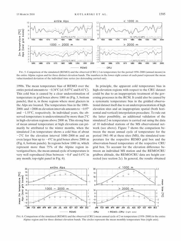
1990s. The mean temperature bias of REMO over the

entire period amounts to 20.348C (cf. 8.078C and 8.418C).

This cold bias is caused by a clear underestimation of

temperature in grid boxes above 1000 m (Fig. 5, bottom

panels), that is, in those regions where most glaciers in

the Alps are located. The temperature bias in the 1000–

2000- and .2000-m elevation intervals amounts to 20.978

and 21.558C, respectively. In individual years, the ob-

served temperature is underestimated by more than 28C

in high-elevation regions above 2000 m. This strong bias

of mean annual temperature at high elevations can pri-

marily be attributed to the winter months, when the

simulated 2-m temperature shows a cold bias of about

228C for the elevation interval 1000–2000 m and an

even larger bias up to 248C in grid boxes above 2000 m

(Fig. 6, bottom panels). In regions below 1000 m, which

represent more than 75% of the Alpine region in-

vestigated here, the mean annual cycle of temperature is

very well reproduced (bias between 20.48 and 0.48C in

any month; top-right panel in Fig. 6).

In principle, the apparent cold temperature bias in

high-elevation regions with respect to the CRU dataset

could be due to an inappropriate treatment of the gov-

erning processes in the RCM. It could also be caused by

a systematic temperature bias in the gridded observa-

tional dataset itself due to an underrepresentation of high

elevation sites and an inappropriate spatial (both hori-

zontal and vertical) interpolation procedure. To rule out

the latter possibility, an additional validation of the

simulated 2-m temperature is carried out using the data

of 10 individual stations of the MS observational net-

work (see above). Figure 7 shows the comparison be-

tween the mean annual cycle of temperature for the

period 1961–90 at these sites (MS), the simulated tem-

perature for the respective REMO grid box and the

observation-based temperature of the respective CRU

grid box. To account for the elevation difference be-

tween an individual MS station and the REMO/CRU

gridbox altitude, the REMO/CRU data are height cor-

rected (see section 2c). In general, the results obtained

FIG. 5. Comparison of the simulated (REMO) and the observed (CRU) 2-m temperature for the period 1958–2000 (annual means) in

the entire Alpine region and for three distinct elevation bands. The numbers in the lower-right corner of each panel represent the mean

value/standard deviation of the individual time series (no detrending carried out).

FIG. 6. Comparison of the simulated (REMO) and the observed (CRU) mean annual cycle of 2-m temperature (1958–2000) in the entire

Alpine region and for three distinct elevation bands. The circles represent the mean monthly temperature bias (right axis).


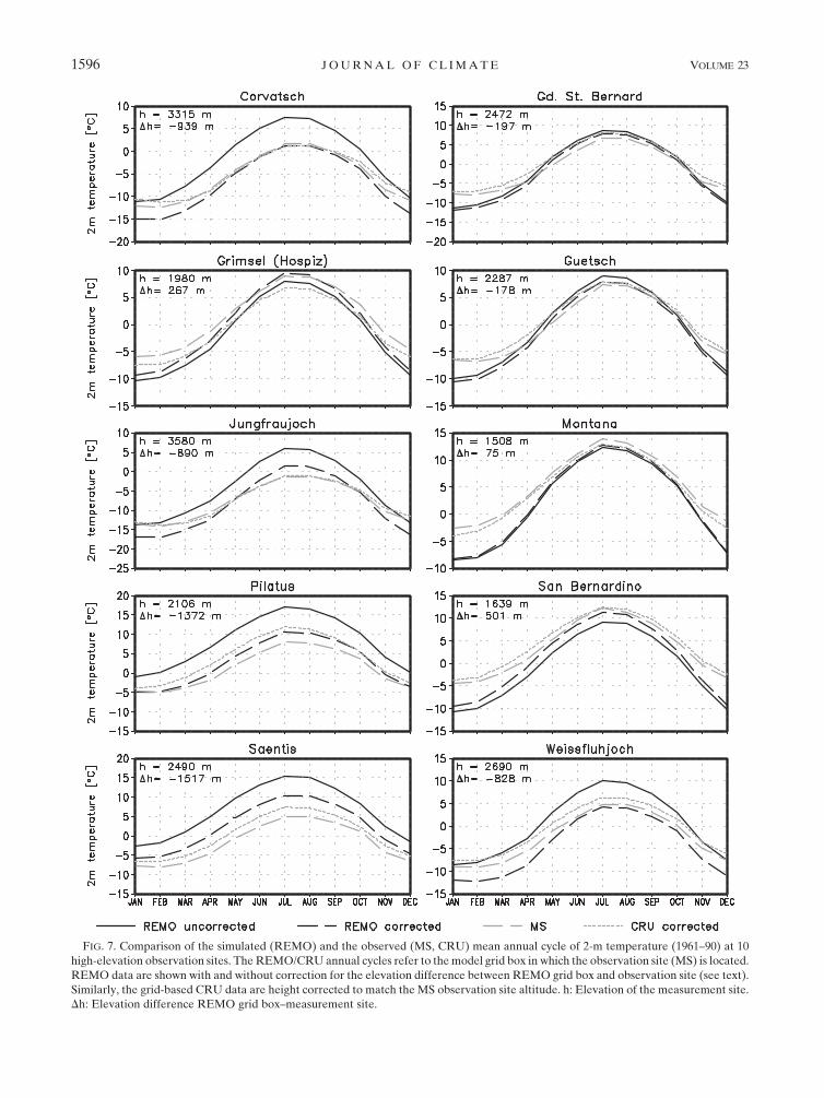
FIG. 7. Comparison of the simulated (REMO) and the observed (MS, CRU) mean annual cycle of 2-m temperature (1961–90) at 10

high-elevation observation sites. The REMO/CRU annual cycles refer to the model grid box in which the observation site (MS) is located.

REMO data are shown with and without correction for the elevation difference between REMO grid box and observation site (see text).

Similarly, the grid-based CRU data are height corrected to match the MS observation site altitude. h: Elevation of the measurement site.

Dh: Elevation difference REMO grid box–measurement site.


for the individual elevation intervals are confirmed in

this analysis. Except for Pilatus and Saentis, the height-

corrected REMO temperature shows a pronounced cold

bias with respect to the MS observations in winter. This is

true for stations that lie above the mean REMO gridbox

altitude (e.g., Corvatsch, Jungfraujoch, and Weissfluhjoch)

and for stations with a lower elevation (e.g., Grimsel and

San Bernardino). Hence, the obvious underestimation

of wintertime temperature is probably not due to wrong

assumptions concerning the temperature lapse rate in this

season (which is applied during the height-correction

procedure) but rather points to a systematic model bias.

In summer, on the other hand, the simulated height-

corrected temperature is relatively close to the MS ob-

servations. The only exceptions are Jungfraujoch, Pilatus,

and Saentis, where REMO shows a positive summer bias

of more than 28C. At these sites the measurement sta-

tion is located at a much higher altitude than the re-

spective REMO grid box and the model bias could

partly be caused by inaccuracies in the height-correction

procedure (i.e., by errors in the temperature lapse rate

assumed for the summer months).

At most sites, the height-corrected temperature of the

CRU dataset approximately corresponds to the MS data.

Exceptions are Grimsel and Pilatus where CRU and MS

disagree by more than 28C during the summer months.

Generally, the pronounced negative wintertime bias of

REMO with respect to the MS observations is larger

than the difference between the two observational data-

sets, which points to a ‘‘true’’ and systematic model bias

rather than to inaccuracies in the reference datasets.

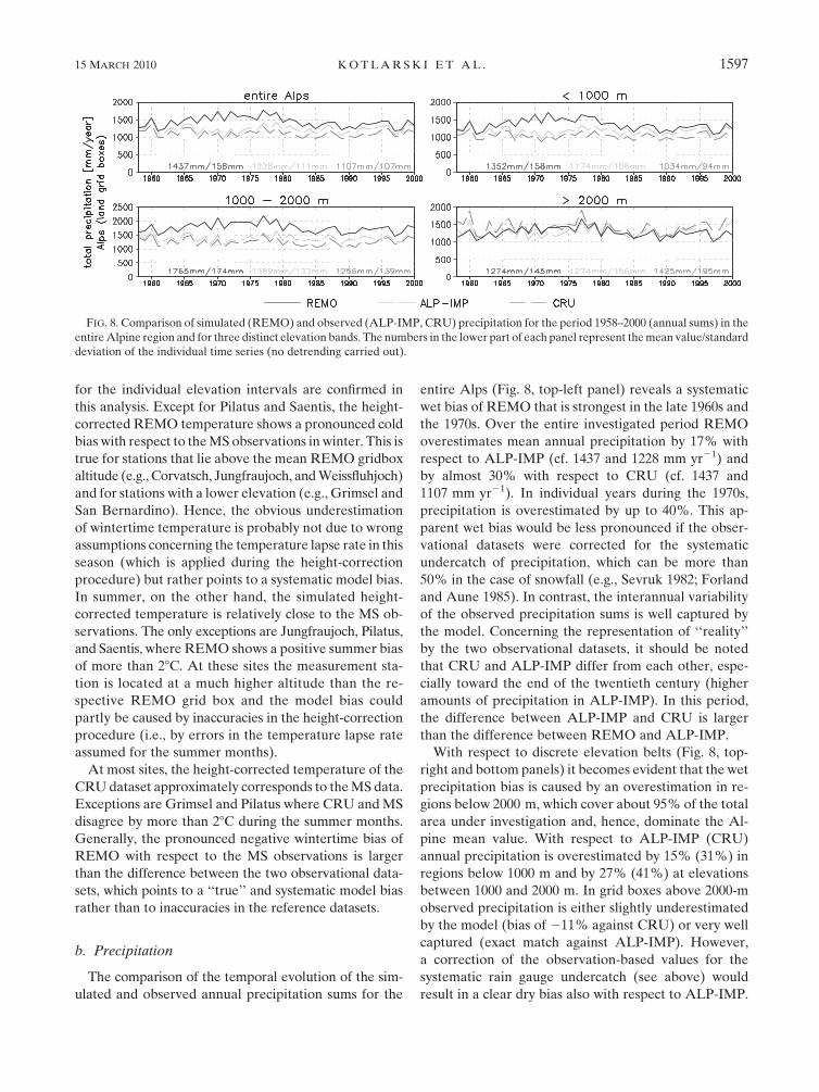
b. Precipitation

The comparison of the temporal evolution of the sim-

ulated and observed annual precipitation sums for the

entire Alps (Fig. 8, top-left panel) reveals a systematic

wet bias of REMO that is strongest in the late 1960s and

the 1970s. Over the entire investigated period REMO

overestimates mean annual precipitation by 17% with

respect to ALP-IMP (cf. 1437 and 1228 mm yr21) and

by almost 30% with respect to CRU (cf. 1437 and

1107 mm yr21). In individual years during the 1970s,

precipitation is overestimated by up to 40%. This ap-

parent wet bias would be less pronounced if the obser-

vational datasets were corrected for the systematic

undercatch of precipitation, which can be more than

50% in the case of snowfall (e.g., Sevruk 1982; Forland

and Aune 1985). In contrast, the interannual variability

of the observed precipitation sums is well captured by

the model. Concerning the representation of ‘‘reality’’

by the two observational datasets, it should be noted

that CRU and ALP-IMP differ from each other, espe-

cially toward the end of the twentieth century (higher

amounts of precipitation in ALP-IMP). In this period,

the difference between ALP-IMP and CRU is larger

than the difference between REMO and ALP-IMP.

With respect to discrete elevation belts (Fig. 8, top-

right and bottom panels) it becomes evident that the wet

precipitation bias is caused by an overestimation in re-

gions below 2000 m, which cover about 95% of the total

area under investigation and, hence, dominate the Al-

pine mean value. With respect to ALP-IMP (CRU)

annual precipitation is overestimated by 15% (31%) in

regions below 1000 m and by 27% (41%) at elevations

between 1000 and 2000 m. In grid boxes above 2000-m

observed precipitation is either slightly underestimated

by the model (bias of 211% against CRU) or very well

captured (exact match against ALP-IMP). However,

a correction of the observation-based values for the

systematic rain gauge undercatch (see above) would

result in a clear dry bias also with respect to ALP-IMP.

FIG. 8. Comparison of simulated (REMO) and observed (ALP-IMP, CRU) precipitation for the period 1958–2000 (annual sums) in the

entire Alpine region and for three distinct elevation bands. The numbers in the lower part of each panel represent the mean value/standard

deviation of the individual time series (no detrending carried out).


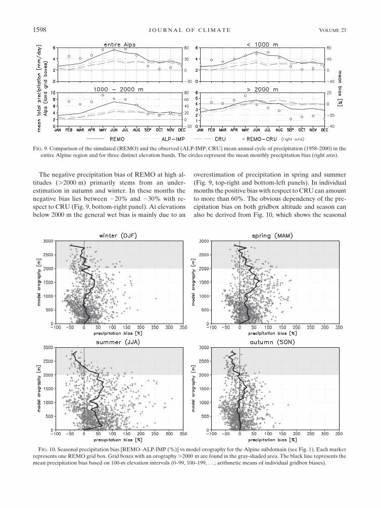
The negative precipitation bias of REMO at high al-

titudes (.2000 m) primarily stems from an under-

estimation in autumn and winter. In these months the

negative bias lies between 220% and 230% with re-

spect to CRU (Fig. 9, bottom-right panel). At elevations

below 2000 m the general wet bias is mainly due to an

overestimation of precipitation in spring and summer

(Fig. 9, top-right and bottom-left panels). In individual

months the positive bias with respect to CRU can amount

to more than 60%. The obvious dependency of the pre-

cipitation bias on both gridbox altitude and season can

also be derived from Fig. 10, which shows the seasonal

FIG. 9. Comparison of the simulated (REMO) and the observed (ALP-IMP, CRU) mean annual cycle of precipitation (1958–2000) in the

entire Alpine region and for three distinct elevation bands. The circles represent the mean monthly precipitation bias (right axis).

FIG. 10. Seasonal precipitation bias [REMO–ALP-IMP (%)] vs model orography for the Alpine subdomain (see Fig. 1). Each marker

represents one REMO grid box. Grid boxes with an orography .2000 m are found in the gray-shaded area. The black line represents the

mean precipitation bias based on 100-m elevation intervals (0–99, 100–199, . . .; arithmetic means of individual gridbox biases).


precipitation bias for each individual grid box against

altitude. The black line in each panel denotes the mean

bias for each 100-m elevation interval (arithmetic mean

of individual gridbox biases). In addition to the general

dependence of the precipitation bias on the altitude,

Fig. 10 also reveals that elevation is not the only con-

trolling factor. The seasonal bias is subject to a consider-

able spread between individual grid boxes of the same

elevation interval. In summertime, for instance, precip-

itation biases in grid boxes above 2000-m range from

260% to 1170% (bottom-left panel). Still, the majority

of high-elevation boxes shows a clear underestimation of

precipitation in summer, autumn, and winter, which is in

some cases larger than 50% (top-left and bottom panels).

With increasing elevation the negative bias generally

becomes more pronounced. In individual high-elevation

grid boxes, precipitation can also be overestimated by

more than 50%. In contrast to this, springtime precip-

itation is overestimated by the model in most grid boxes

independent of their altitude (top-right panel). In all

seasons the maximum mean precipitation bias is found at

altitudes between 1500 and 1800 m. The largest positive

biases arise in the summer season and below 2000 m,

with an overestimation of precipitation by more than

250% in individual grid boxes (bottom-left panel).

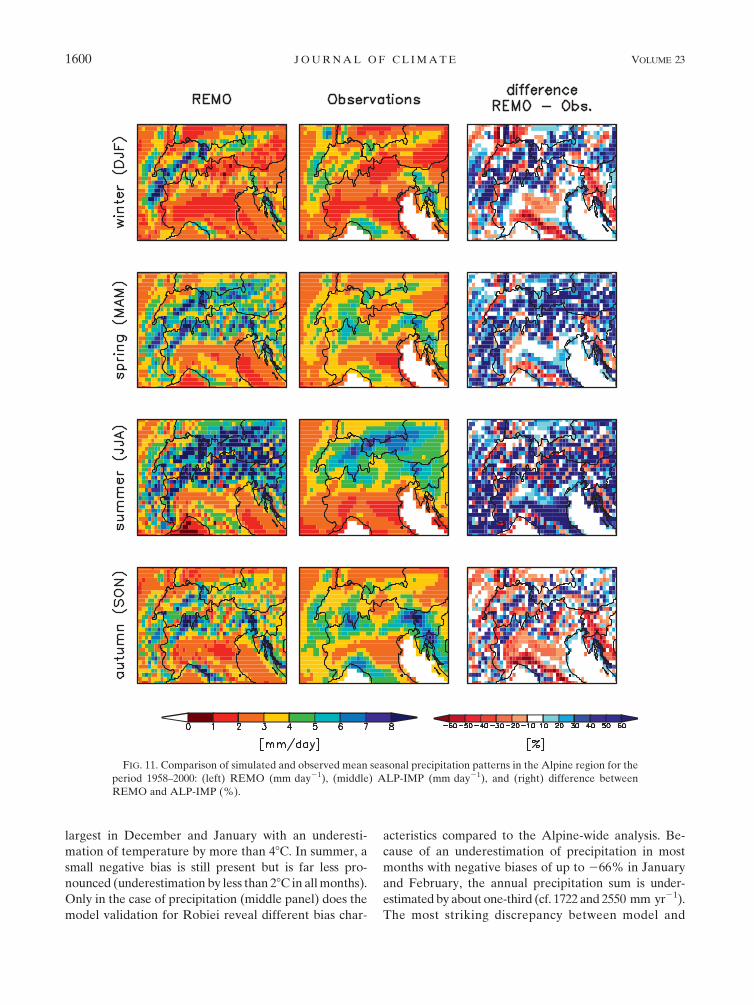
The strong overestimation of summertime precip-

itation in large parts of the study region also becomes

evident when comparing the simulated and the observed

(ALP-IMP) spatial patterns of mean seasonal pre-

cipitation (Fig. 11). A large number of grid boxes in the

Alpine region show a clear positive bias of more than

60% in summer. Still, precipitation in regions along the

southern Alpine ridge (southern Switzerland) and along

the ridge of the Jura Mountains (northwestern border

of Switzerland) is considerably underestimated by the

model. This discrepancy between the precipitation bias

at grid boxes located along local orographic maxima

(negative bias) and their neighboring regions (strong

positive bias) becomes even more evident in winter (top

panels in Fig. 11). Apparently, the model systematically

dislocates precipitation from ridges to the forelands

causing a negative precipitation bias at high-elevation

sites in all seasons. The large-scale seasonal precipitation

patterns (highest precipitation sums in the Alpine region

except for some dry inner-alpine regions, lower sums in

the surrounding regions) are still well captured by the

model.

c. Global radiation

Global radiation often constitutes the primary source

of melt energy on glaciers and plays a key role for glacier

mass balance (e.g., Oerlemans 2001). An accurate de-

scription of the global radiation flux is therefore of high

importance in mass balance modeling. In the RCM

downscaling approach presented in Part II, the global

radiation flux as simulated by REMO is used as an input

for the distributed MBM.

Figure 12 presents a comparison between the simu-

lated (REMO) and the observed (MS) mean annual

cycle of global radiation for 10 high-elevation measure-

ment sites of the Swiss automatic network, all of them

located above 1300 m. Model and observations are in

good agreement with respect to the basic characteristics

of the annual cycle (mean value and amplitude). Still,

important and systematic model biases arise in individual

seasons. At all sites the mean monthly radiation bias

(circles in Fig. 12) is subject to a pronounced variability

on a monthly basis with maximum values in summer

(July or August, depending on the site, but positive in all

cases) and a minimum in spring (March or April, de-

pending on the site as well, but negative in all cases). At

most stations the positive radiation bias in summer

amounts to several tens of watts per meters squared with

maximum values up to 60 W m22 (July at Pilatus). In

contrast to this, a systematic negative bias of the simu-

lated global radiation flux seems to prevail in winter and

especially in spring. Here, observations are underesti-

mated by more than 50 W m22 at individual stations

(Corvatsch, Guetsch, Jungfraujoch, and Weissfluhjoch).

The only exception is the valley station of Ulrichen

where the simulated springtime global radiation flux

corresponds very well to the observations and negative

biases are smaller than 20 W m22. At very high altitudes

(Corvatsch, Gd. St. Bernard, Jungfraujoch, Saentis, and

Weissfluhjoch), the combination of a negative radiation

bias in spring and a positive summer bias results in

a backward shift of the annual maximum of global ra-

diation by 1–2 months from April–May to June–July in

the model simulation compared to observations.

d. Focus Robiei

In addition to the Alpine-wide analysis presented

above, the performance of REMO is assessed in detail

for the site of Robiei. This station is located close to

Gries and Basodino Glacier, the two glaciers under in-

vestigation in Part II of this study. Figure 13 shows a

comparison of the simulated annual cycle for tempera-

ture, precipitation, and global radiation against Robiei

station data (and against CRU in case of temperature)

for the period 1991–2000. This analysis basically con-

firms the results of the Alpine-wide model evaluation:

systematic model biases that were discovered on the

Alpine scale are also found for the specific site of Robiei.

For instance, REMO strongly underestimates winter-

time temperature with respect to the Robiei station data

and the respective CRU grid box (left panel). Biases are


largest in December and January with an underesti-

mation of temperature by more than 48C. In summer, a

small negative bias is still present but is far less pro-

nounced (underestimation by less than 28C in all months).

Only in the case of precipitation (middle panel) does the

model validation for Robiei reveal different bias char-

acteristics compared to the Alpine-wide analysis. Be-

cause of an underestimation of precipitation in most

months with negative biases of up to 266% in January

and February, the annual precipitation sum is under-

estimated by about one-third (cf. 1722 and 2550 mm yr21).

The most striking discrepancy between model and

FIG. 11. Comparison of simulated and observed mean seasonal precipitation patterns in the Alpine region for the

period 1958–2000: (left) REMO (mm day21), (middle) ALP-IMP (mm day21), and (right) difference between

REMO and ALP-IMP (%).


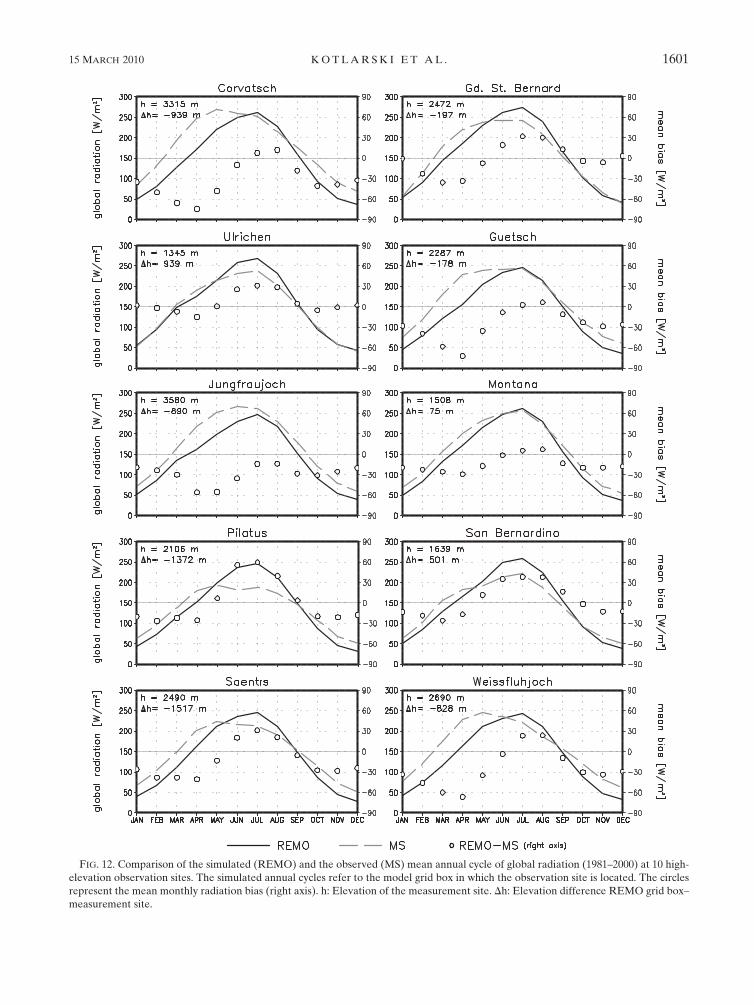
FIG. 12. Comparison of the simulated (REMO) and the observed (MS) mean annual cycle of global radiation (1981–2000) at 10 high-

elevation observation sites. The simulated annual cycles refer to the model grid box in which the observation site is located. The circles

represent the mean monthly radiation bias (right axis). h: Elevation of the measurement site. Dh: Elevation difference REMO grid box–

measurement site.


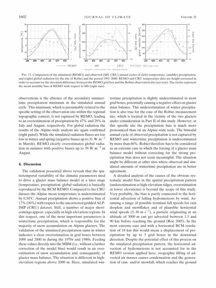
observations is the absence of the secondary summer-

time precipitation minimum in the simulated annual

cycle. This minimum, which is presumably related to the

specific setting of the observation site within the regional

topographic context, is not captured by REMO, leading

to an overestimation of precipitation by 47% and 29% in

July and August, respectively. For global radiation the

results of the Alpine-wide analysis are again confirmed

(right panel). While the simulated radiation fluxes are too

low in winter and spring (negative biases up to 31 W m22

in March), REMO clearly overestimates global radia-

tion in summer with positive biases up to 39 W m22 in

August.

4. Discussion

The validation presented above reveals that the spa-

tiotemporal variability of the climatic parameters used

to drive a glacier mass balance model at a later stage

(temperature, precipitation, global radiation) is basically

reproduced by the RCM REMO. Compared to the CRU

dataset the Alpine mean temperature is underestimated

by 0.348C. Annual precipitation shows a positive bias of

17% (30%) with respect to the uncorrected gridded ALP-

IMP (CRU) dataset. Still, a number of major short-

comings appear, especially in high-elevation regions. In

this respect, one of the most important parameters is

wintertime precipitation, which is responsible for the

majority of snow accumulation on Alpine glaciers. The

validation of the simulated precipitation sums in winter

indicates a clear overestimation in grid boxes between

1000 and 2000 m during the 1970s and 1980s. Feeding

these values directly into the MBM (i.e., without a further

correction of the model bias) would result in an over-

estimation of snow accumulation and, consequently, of

glacier mass balance. The situation is different in high-

elevation regions above 2000 m. Here, simulated win-

tertime precipitation is slightly underestimated in most

grid boxes, potentially causing a negative effect on glacier

mass balance. This underestimation of winter precipita-

tion is also true for the case of the Robiei measurement

site, which is located in the vicinity of the two glaciers

under consideration in Part II of this study. However, at

this specific site the precipitation bias is much more

pronounced than on an Alpine-wide scale. The bimodal

annual cycle of observed precipitation is not captured by

REMO and wintertime precipitation is underestimated

by more than 60%. Robiei therefore has to be considered

as an extreme case in which the forcing of a glacier mass

balance model without correcting for the strong pre-

cipitation bias does not seem meaningful. The situation

might be different at other sites where observed and sim-

ulated amounts of wintertime precipitation are in better

agreement.

A detailed analysis of the causes of the obvious sys-

tematic model bias in the spatial precipitation pattern

(underestimation at high-elevation ridges, overestimation

at lower elevations) is beyond the scope of this study.

Very probably, the bias is partly connected to the hori-

zontal advection of falling hydrometeors by wind. As-

suming a range of possible terminal fall speeds for rain

droplets and snowflakes and of plausible horizontal

wind speeds (5–30 m s21), a particle originating at an

altitude of 3000 m can get advected between 1.5 and

90 km before reaching the ground (Roe 2005). In the

most extreme case and with a horizontal RCM resolu-

tion of 18 km this would mean a displacement of pre-

cipitation by up to 5 grid boxes in the downwind

direction. Despite the potential effect of this process on

the simulated precipitation pattern, the horizontal ad-

vection of hydrometeors is not accounted for in the

REMO version applied here: orographic lifting of ad-

vected air masses causes condensation and the genera-

tion of rain- and/or snowfall, which reaches the ground

FIG. 13. Comparison of the simulated (REMO) and observed (MS, CRU) annual cycles of (left) temperature, (middle) precipitation,

and (right) global radiation for the site of Robiei and the period 1991–2000. REMO and CRU temperature data are height corrected in

order to account for the elevation difference between the REMO grid box and the Robiei observation site (see text). The circles represent

the mean monthly bias of REMO with respect to MS (right axis).


in the same time step at the base of the vertical gridbox

column. This neglect of the advection of falling pre-

cipitation can lead to a systematic overestimation of

precipitation on the windward slopes and an under-

estimation downwind. The recent development of an

online advection scheme for precipitation (Gottel 2009)

shows that the explicit consideration of the drift of fall-

ing hydrometeors can considerably reduce the pre-

cipitation bias of REMO at high altitudes. Gottel (2009)

applied REMO at a horizontal resolution of about

10 km 3 10 km, but it can be expected that a similar

effect, though less pronounced, would appear for the

resolution applied in the present study (18 km 3 18 km).

A further reason for the elevation-dependent pre-

cipitation bias could be the use of a nonsmoothed model

topography, which can lead to sharp gradients of to-

pography between adjacent grid boxes and the genera-

tion of small-scale gravity waves. On the coarse model

grid scale, the latter can only be represented in an ap-

proximate manner which potentially causes a disloca-

tion of zones of up- and downdraft (e.g., Gaßmann

2002). This, in turn, could result in a too early conden-

sation of atmospheric water vapor and a too early oc-

currence of rain- and snowfall when humid air masses

are lifted by an orographic obstacle.

Besides the model’s precipitation bias a further im-

portant point for mass balance modeling is the cold

temperature bias at high altitudes for most parts of the

year. This bias would generally lead to an overestimation

of the fraction of solid precipitation (snowfall) and,

hence, to an increase in snow accumulation with a positive

effect on glacier mass balance. The general underesti-

mation of temperature would also cause a reduction of

melt rates through a reduced flux of sensible heat toward

the glacier surface, resulting in a positive bias of glacier

mass balance. However, summer temperature biases

(which are less pronounced in REMO) are much more

important for this effect than inaccuracies in modeled

winter temperature (which is strongly underestimated

by REMO). A positive effect on glacier mass balance

can also be assumed for the negative bias of springtime

global radiation at high-elevation sites. This phenome-

non can possibly be attributed to errors in the simulated

cloud cover since clouds exert a primary influence on

the incoming surface radiation fluxes. A possible over-

estimation of springtime cloud cover could be connected

to the overestimation of precipitation in most grid boxes

in this season (see above), indicating that a general

positive bias of large-scale humidity might be a further

possible reason for the precipitation bias of REMO.

Model deficiencies related to clouds and their in-

fluence on radiative processes are probably also re-

sponsible for the systematic overestimation of global

radiation at high-elevation sites in summer. Here, the

lower radiation flux in the observational dataset might

be connected to orographically induced convective ac-

tivity and the formation of convective clouds. These

processes are not explicitly resolved by the RCM. They

are treated by the model’s convection parameterization

scheme in a strongly simplified manner and without a

direct influence of convective clouds on radiative pro-

cesses. Concerning the larger observed solar radiation

flux in winter and spring, a further reason could be

multiple reflection of solar radiation on surrounding

snow-covered slopes, a process that is also not consid-

ered in REMO.

Finally, it should be mentioned that in the region of

interest (in high-altitude Alpine terrain) the coverage of

meteorological stations is usually very sparse and errors

of meteorological measurements themselves are largest.

The uncertainty of observation-based datasets used for

model validation is thus relatively large, especially in the

case of precipitation.

5. Conclusions

The present study investigates the potential of using

RCM output as an atmospheric forcing for distributed

glacier mass balance models in the European Alps, a

region with a complex topography and a high spatial

variability of atmospheric quantities. The detailed vali-

dation of those parameters that will serve as input to the

mass balance model (near-surface air temperature, pre-

cipitation, and global radiation) shows that the basic

spatial and temporal variabilities of all three parameters

are reproduced by REMO. This provides confidence in

the general applicability of REMO data for mass bal-

ance modeling. However, regarding the specific ques-

tions raised in the introductory chapter, important and

systematic RCM deficiencies are detected at high ele-

vations. If applied without further bias correction, some

of these deficiencies have a high potential to cause errors

in the subsequent simulation of glacier mass balance

[viz., the bias of winter precipitation (positive or nega-

tive, depending primarily on gridbox altitude), the neg-

ative temperature bias in winter, and the overestimation

of summertime global radiation]. It is thus recommended

to account for these known deficiencies by applying cor-

rection procedures before using the RCM output for

subsequent impact studies. Implicitly, such a correction

could also account for inconsistencies in the atmospheric

forcing related to different surface conditions in the

RCM and the MBM, respectively (e.g., ice-free surface

in the RCM versus ice-covered surface in the MBM).

Concerning climate change studies, the general question

arises whether RCM biases are stationary in time


(i.e., whether the same correction can be applied for today’s

and for future climatic conditions). There is strong evidence

that this assumption is not necessarily valid (Christensen

et al. 2008). We also fully recognize that different RCMs

might perform differently in high-mountain topography.

These aspects have been and are still under investigation

in several model intercomparison studies such as the

Prediction of Regional Scenarios and Uncertainties for

Defining European Climate Change Risks and Effects

(PRUDENCE; Christensen et al. 2007) and Ensemble-

based Predictions of Climate Changes and their Impacts

(ENSEMBLES) (Hewitt 2005). We start here with just

one single RCM in order to investigate the principal

challenges of an RCM–MBM coupling.

Whether RCM biases are corrected prior to forcing an

MBM or not, a further downscaling of the RCM output

to the scale required by distributed MBMs is necessary.

Although the RCM resolution used in the present study

(approximately 18 km 3 18 km) is comparatively high,

it does not yet correspond to the MBM scale. The same

is true for most other impact models (e.g., catchment-

scale water balance models). A straightforward way to

bridge the apparent scale gap is the further redistri-

bution of atmospheric quantities on the RCM subgrid

scale using high-resolution observational datasets (local

scaling of precipitation) and/or a known altitudinal de-

pendence of parameters like precipitation and temper-

ature. Local scaling of RCM-simulated precipitation

could also be combined with a bias correction as applied

in Widmann et al. (2003) and Fruh et al. (2006). For the

present two-part study we have decided to first present

the original RCM output in Part I (in order to detect

principle RCM shortcomings) and to bridge the scale

gap for the specific application of the impact model af-

terward (Part II).

Despite the encountered RCM biases at high eleva-

tions, a number of obvious advantages justify the use of

RCM data as an input to glacier mass balance models.

Especially in regions with a low density of meteorolog-

ical measurement networks, RCMs can provide useful

information on the scale of entire mountain ranges. This,

however, implies that systematic model biases are known

and could be corrected for. Furthermore, the develop-

ment of an RCM–MBM interface will facilitate the use of

RCM climate change scenarios for the assessment of fu-

ture changes in glacier area and volume. One advantage

of this physical downscaling method compared to a sta-

tistical downscaling of coarse-resolution GCM climate

change signals to the sites of individual glaciers (e.g.,

Schneeberger et al. 2001; Reichert et al. 2002; Radic and

Hock 2006) is that an RCM responds in a physically

consistent way to different external forcings, such as

changes in atmospheric greenhouse gas concentrations

(Wilby et al. 2000). Unless the RCM output is being

postprocessed on an individual-parameter basis (e.g.,

bias correction for individual output parameters) the

relation between the simulated values of, for example,

precipitation, air temperature, and radiation is physi-

cally consistent and meaningful. The full potential of

such an approach could only be exploited with an MBM

that is based on the calculation of the complete surface

energy balance and that considers the respective prog-

nostic variables of the RCM.

The setup and the testing of the RCM–MBM interface

for two glaciers of the Swiss mass balance will be pre-

sented in Part II.

Acknowledgments. This study received financial sup-

port from a grant by the Swiss National Science Foun-

dation (Grant 21-105214/1), the EU-funded action COST

719 (BBW C001.0041), and the International Max Planck

Research School on Earth System Modelling (IMPRS-

ESM). We thank Thomas Bosshard for his support in data

analysis and four anonymous reviewers for their helpful

and constructive comments.

REFERENCES

Arnold, N. S., I. C. Willis, M. J. Sharp, K. S. Richards, and

W. J. Lawson, 1996: A distributed surface energy-balance

model for a small valley glacier. I. Development and testing

for Haut Glacier d’Arolla, Valais, Switzerland. J. Glaciol., 42,

77–89.

Brock, B. W., I. C. Willis, M. J. Sharp, and N. S. Arnold, 2000:

Modelling seasonal and spatial variations in the surface energy

balance of Haut Glacier d’Arolla, Switzerland. Ann. Glaciol.,

31, 53–62.

Christensen, J. H., and O. B. Christensen, 2007: A summary of the

PRUDENCE model projections of changes in European cli-

mate by the end of this century. Climatic Change, 81, 7–30.

——, T. R. Carter, M. Rummukainen, and G. Amanatidis, 2007:

Evaluating the performance and utility of regional climate

models: The PRUDENCE project. Climatic Change, 81, 1–6.

——, F. Boberg, O. B. Christensen, and P. Lucas-Picher, 2008: On

the need for bias correction of regional climate change pro-

jections of temperature and precipitation. Geophys. Res. Lett.,

35, L20709, doi:10.1029/2008GL035694.

Davies, H. C., 1976: A lateral boundary formulation for multi-level

prediction models. Quart. J. Roy. Meteor. Soc., 102, 405–418.

Deque, M., and Coauthors, 2005: Global high resolution versus

Limited Area Model climate change projections over Europe:

Quantifying confidence level from PRUDENCE results. Cli-

mate Dyn., 25, 653–670.

Efthymiadis, D., P. Jones, K. Briffa, I. Auer, R. Bohm, W. Schoner,

C. Frei, and J. Schmidli, 2006: Construction of a 10-min-

gridded precipitation data set for the Greater Alpine Region

for 1800-2003. J. Geophys. Res., 111, D01105, doi:10.1029/

2005JD006120.

Forland, E. J., and B. Aune, 1985: Comparison of Nordic methods

for point precipitation correction. Correction of Precipitation

Measurements, Zurcher Geographische Schriften 23, B. Sevruk,

Ed., Geographisches Institut ETH Zurich, 239–244.


Frei, C., J. H. Christensen, M. Deque, D. Jacob, R. G. Jones, and

P. L. Vidale, 2003: Daily precipitation statistics in regional

climate models: Evaluation and intercomparison for the

European Alps. J. Geophys. Res., 108, 4124, doi:10.1029/

2002JD002287.

Fruh, B., J. W. Schipper, A. Pfeiffer, and V. Wirth, 2006: A prag-

matic approach for downscaling precipitation in alpine-scale

complex terrain. Meteor. Z., 15, 631–646.

Gaßmann, A., 2002: Numerische Verfahren in der nichthy-

drostatischen Modellierung und ihr Einfluss auf die Gute der

Niederschlagsvorhersage (Numerical methods in nonhydrostatic

modelling and their influence on the quality of the precipitation

forecast). Ph.D. thesis, University of Bonn, 91 pp.

Giorgi, F., 1990: Simulation of regional climate using a limited

area model nested in a general circulation model. J. Climate, 3,

941–963.

Gottel, H., 2009: Einfluss der nichthydrostatischen Modellierung

und der Niederschlagsverdriftung auf die Ergebnisse region-

aler Klimamodellierung (Influence of nonhydrostatic model-

ling and precipitation drift on regional climate model results).

Ph.D. thesis, University of Hamburg/Max Planck Institute for

Meteorology, Hamburg, Germany, 126 pp.

Haeberli, W., and M. Hoelzle, 1995: Application of inventory data

for estimating characteristics of and regional climate-change

effects on mountain glaciers: A pilot study with the European

Alps. Ann. Glaciol., 21, 206–212.

Hewitt, C., 2005: The ENSEMBLES Project—Providing ensemble-

based predictions of climate changes and their impacts. EGGS

Newsl., 13, 22–25.

Hock, R., 1999: A distributed temperature-index ice- and snowmelt

model including potential direct solar radiation. J. Glaciol., 45,

101–111.

Jacob, D., 2001: A note to the simulation of the annual and inter-

annual variability of the water budget over the Baltic Sea

drainage basin. Meteor. Atmos. Phys., 77, 61–73.

——, and R. Podzun, 1997: Sensitivity studies with the regional

climate model REMO. Meteor. Atmos. Phys., 63, 119–129.

——, and Coauthors, 2001: A comprehensive model inter-comparison

study investigating the water budget during the BALTEX-

PIDCAP period. Meteor. Atmos. Phys., 77, 19–43.

——, and Coauthors, 2007: An inter-comparison of regional cli-

mate models for Europe: Model performance in present-day

climate. Climatic Change, 81, 31–52.

Klok, E. J., and J. Oerlemans, 2002: Model study of the spatial

distribution of the energy and mass balance of Morter-

atschgletscher, Switzerland. J. Glaciol., 48, 505–518.

Kotlarski, S., 2007: A subgrid glacier parameterisation for use in

regional climate modelling. Ph.D. thesis, Reports on Earth

System Science, Rep. 42, Max Planck Institute for Meteorol-

ogy, Hamburg, Germany, 199 pp. [Available online at http://

www.mpimet.mpg.de/fileadmin/publikationen/Reports/WEB_

BzE_42.pdf.]

——, A. Block, U. Bohm, D. Jacob, K. Keuler, R. Knoche,

D. Rechid, and A. Walter, 2005: Regional climate model

simulations as input for hydrological applications: Evaluation

of uncertainties. Adv. Geosci., 5, 119–125.

Machguth, H., F. Paul, M. Hoelzle, and W. Haeberli, 2006: Dis-

tributed glacier mass-balance modelling as an important

component of modern multi-level glacier monitoring. Ann.

Glaciol., 43, 335–343.

Majewski, D., 1991: The Europa-Modell of the Deutscher Wetter-

dienst. Vol. 2, ECMWF Seminar on Numerical Methods in

Atmospheric Models, ECMWF, 147–191.

McGregor, J. L., 1997: Regional Climate Modelling. Meteor. At-

mos. Phys., 63, 105–117.

Mitchell, T. D., T. R. Carter, P. D. Jones, M. Hulme, and M. New,

2004: A comprehensive set of high-resolution grids of monthly

climate for Europe and the globe: The observed record (1901-

2000) and 16 scenarios (2001-2100). Tyndall Centre Working

Paper No. 55, Tyndall Centre for Climate Change Research,

30 pp.

New, M., M. Hulme, and P. Jones, 2000: Representing twentieth-

century space–time climate variability. Part II: Develop-

ment of 1901–96 monthly grids of terrestrial surface climate.

J. Climate, 13, 2217–2238.

Oerlemans, J., 2001: Glaciers and Climate Change. A. A. Balkema,

148 pp.

Paul, F., and S. Kotlarski, 2010: Forcing a distributed glacier mass

balance model with the regional climate model REMO. Part II:

Downscaling strategy and results for two Swiss glaciers.

J. Climate, 23, 1607–1620.

——, A. Kaab, M. Maisch, T. Kellenberger, and W. Haeberli,

2004: Rapid disintegration of Alpine glaciers observed with

satellite data. Geophys. Res. Lett., 31, L21402, doi:10.1029/

2004GL020816.

Radic, V., and R. Hock, 2006: Modeling future glacier mass balance

and volume changes using ERA-40 reanalysis and climate

models: A sensitivity study at Storglaciaren, Sweden. J. Geo-

phys. Res., 111, F03003, doi:10.1029/2005JF000440.

Raper, S. C. B., and R. J. Braithwaite, 2006: Low sea level rise

projections from mountain glaciers and icecaps under global

warming. Nature, 439, 311–313.

Reichert, B. K., L. Bengtsson, and J. Oerlemans, 2002: Recent

glacier retreat exceeds internal variability. J. Climate, 15,

3069–3081.

Roe, G. H., 2005: Orographic precipitation. Annu. Rev. Earth

Planet. Sci., 33, 645–671.

Roeckner, E., and Coauthors, 1996: The atmospheric general cir-

culation model ECHAM-4: Model description and simulation

of present-day climate. Rep. 218, Max Planck Institute for

Meteorology, Hamburg, Germany, 90 pp.

Schneeberger, C., O. Albrecht, H. Blatter, M. Wild, and R. Hock,

2001: Modelling the response of glaciers to a doubling in

atmospheric CO2: A case study of Storglaciaren, northern

Sweden. Climate Dyn., 17, 825–834.

Schwarb, M., 2000: The Alpine precipitation climate—Evaluation

of a high-resolution analysis scheme using comprehensive

rain-gauge data. Ph.D. thesis, Swiss Federal Institute of

Technology, Zurich, Switzerland, 131 pp.

Semmler, T., and D. Jacob, 2004: Modeling extreme precipitation

events—A climate change simulation for Europe. Global

Planet. Change, 44, 119–127.

Sevruk, B., 1982: Methods of correction for systematic errors in

point precipitation measurement for operational use. WMO

Hydrol. Rep. 21, WMO 589, WMO, 91 pp.

Simmons, A. J., and D. M. Burridge, 1981: An energy and angular-

momentum conserving vertical finite-difference scheme and

hybrid vertical coordinate. Mon. Wea. Rev., 109, 758–766.

Stahl, K., R. D. Moore, J. M. Shea, D. Hutchinson, and A. J. Cannon,

2008: Coupled modelling of glacier and streamflow response to

future climate scenarios. Water Resour. Res., 44, W02422,

doi:10.1029/2007WR005956.

Uppala, S. M., and Coauthors, 2005: The ERA-40 Re-Analysis.

Quart. J. Roy. Meteor. Soc., 131, 2961–3012.

Van de Wal, R. S. W., and M. Wild, 2001: Modelling the response of

glaciers to climate change by applying volume-area scaling in


combination with a high resolution GCM. Climate Dyn., 18,

359–366.

WGMS, 1989: World glacier inventory—Status 1988. W. Haeberli

et al., Eds., World Glacier Monitoring Service, 458 pp.

——, 2008: Global glacier changes: Facts and figures. M. Zemp

et al., Eds., World Glacier Monitoring Service, 88 pp.

Widmann, M., C. S. Bretherton, and E. P. Salathe Jr., 2003: Sta-

tistical precipitation downscaling over the northwestern United

States using numerically simulated precipitation as a predictor.

J. Climate, 16, 799–816.

Wilby, R. L., L. E. Hay, W. J. Gutowski Jr., R. W. Arritt, E. S. Takle,

Z. Pan, G. Leavesley, and M. P. Clark, 2000: Hydrological re-

sponses to dynamically and statistically downscaled climate

model output. Geophys. Res. Lett., 27, 1199–1202.

Zemp, M., M. Hoelzle, and W. Haeberli, 2007: Distributed

modelling of the regional climatic equilibrium line altitude of

glaciers in the European Alps. Global Planet. Change, 56,

83–100.

——, F. Paul, M. Hoelzle, and W. Haeberli, 2008: Glacier fluctu-

ations in the European Alps 1850–2000: An overview and

spatio-temporal analysis of available data. The Darkening

Peaks: Glacial Retreat in Scientific and Social Context, B. Orlove,

E. Wiegandt, and B. Luckman, Eds., University of California

Press, 152–167.


Documents

Forcing a Distributed Glacier Mass Balance Model with the