Forecast Skill of Synoptic Conditions Associated with

Forecast Skill of Synoptic Conditions Associated with Santa Ana Windsin Southern California

CHARLES JONES

Institute for Computational Earth System Science, University of California, Santa Barbara, Santa Barbara, California

FRANCIS FUJIOKA

U.S. Department of Agriculture, Forest Service, Pacific Southwest Research Station, Riverside, California

LEILA M. V. CARVALHO

Institute for Computational Earth System Science, and Department of Geography, University of California,

Santa Barbara, Santa Barbara, California

(Manuscript received 2 March 2010, in final form 20 May 2010)

ABSTRACT

Santa Ana winds (SAW) are synoptically driven mesoscale winds observed in Southern California usually

during late fall and winter. Because of the complex topography of the region, SAW episodes can sometimes be

extremely intense and pose significant environmental hazards, especially during wildfire incidents. A simple

set of criteria was used to identify synoptic-scale conditions associated with SAW events in the NCEP–

Department of Energy (DOE) reanalysis. SAW events start in late summer and early fall, peak in December–

January, and decrease by early spring. The typical duration of SAW conditions is 1–3 days, although extreme

cases can last more than 5 days. SAW events exhibit large interannual variations and possible mechanisms

responsible for trends and low-frequency variations need further study. A climate run of the NCEP Climate

Forecast System (CFS) model showed good agreement and generally small differences with the observed

climatological characteristics of SAW conditions.

Nonprobabilistic and probabilistic forecasts of synoptic-scale conditions associated with SAW were derived

from NCEP CFS reforecasts. The CFS model exhibits small systematic biases in sea level pressure and surface

winds in the range of a 1–4-week lead time. Several skill measures indicate that nonprobabilistic forecasts of

SAW conditions are typically skillful to about a 6–7-day lead time and large interannual variations are ob-

served. NCEP CFS reforecasts were also applied to derive probabilistic forecasts of synoptic conditions

during SAW events and indicate skills to about a 6-day lead time.

1. Introduction

Southern California is characterized by complex to-

pography that fundamentally influences the climate of the

region. During fall and winter, a downslope flow known

locally as the Santa Ana winds (SAW) occasionally affects

Southern California (Lea 1969; McCutchan and Schroeder

1973; Small 1995; Raphael 2003; Hughes and Hall 2009).

A surface high pressure system over the Great Basin and

a low pressure system offshore of Southern California

induce a synoptic pressure gradient that drives surface

winds into the Los Angeles Basin from the northeast

quadrant (Whiteman 2000). The winds can squeeze

through the Santa Clara River Valley and the Cajon and

Banning Passes that open to the Los Angeles Basin, with

wind speeds that can reach hurricane strength in some

locations (Fig. 1). During SAW occurrences, it has been

noted that offshore flow can sometimes appreciably ex-

tend to adjacent waters of the California Bight and parts

of Baja California with strong surface wind jets, dust,

and wildfire smoke plumes, substantially modifying ther-

modynamical, upwelling, and biophysical processes within

the coastal waters (Lynn and Svejkovsky 1984; Castro

et al. 2003; Hu and Liu 2003; Trasvina et al. 2003; Sosa-

Avalos et al. 2005; Castro et al. 2006).

Corresponding author address: Dr. Charles Jones, Institute for

Computational Earth System Science, University of California,

Santa Barbara, Santa Barbara, CA 93106.

E-mail: [email protected]

4528 M O N T H L Y W E A T H E R R E V I E W VOLUME 138

DOI: 10.1175/2010MWR3406.1

� 2010 American Meteorological Society

Previous studies based on weather station data and/or

coarse synoptic weather charts have shown that SAW

occurrences are more frequent in fall and winter months

with peak activity in December and January. Usually,

offshore winds tend to pick up in the morning hours during

SAW events and may persist throughout the day unless

interactions with sea-breeze circulations occur. Climato-

logical studies of SAW include Raphael (2003), who used

33 yr of daily weather maps and a subjective method to

identify SAW occurrences. Conil and Hall (2006) per-

formed simulations with a mesoscale numerical model and

employed an objective classification scheme to demon-

strate that SAW is one of three distinct modes of weather

regimes in Southern California.

One of the most notorious environmental hazards

associated with SAW is wildfire (Schroeder and Buck

1970; Small 1995; Westerling et al. 2003). The intense

downslope winds frequently become hot and dry de-

scending to lower elevations, rapidly increasing the ig-

nitability of fuels and the spread of fire so as to make

predictions of wildfire behavior and fire fighting ex-

tremely difficult (Schroeder et al. 1964, 264–274; Ryan

1969; Minnich 1987; Keeley and Fotheringham 2001;

Moritz 2003; Westerling et al. 2003; Keeley et al. 2004;

Miller and Schlegel 2006). Transport of wildfire smoke

and desert dust can also dramatically alter visibility and air

quality with serious health, social, and economic conse-

quences (Svejkovsky 1985; Reheis and Kihl 1995; Corbett

1996; Lu et al. 2003; Westerling et al. 2003; Phuleria et al.

2005; Wu et al. 2006).

This paper is part of an ongoing research effort to fur-

ther understand the dynamics and predictability of SAW

and its local environmental impacts such as wildfires and

interactions with coastal waters of Southern California.

Here we focus on the synoptic-scale conditions that lead

to Santa Ana winds; namely, the development of the

surface high pressure over the Great Basin, surface low

pressure off the coast of Southern California, and north-

easterly winds over the Los Angeles Basin. Three specific

objectives focus on aspects of SAW at the synoptic scale.

First, the climatological properties of the synoptic-scale

conditions associated with SAW are assessed. This is ac-

complished using the National Centers for Environmental

Prediction–Department of Energy (NCEP–DOE) rean-

alysis and a climate run of the NCEP Climate Forecast

System (CFS) model. Second, the forecast skill of synoptic-

scale conditions associated with SAW is investigated.

Ideally, one would like to investigate this problem us-

ing a large sample of forecasts derived from an opera-

tional numerical weather prediction model with high

spatial resolution. Although NCEP routinely uses sev-

eral mesoscale forecast models [e.g., North American

Mesoscale (NAM), 12 km; Rapid Update Cycle (RUC),

13 km and 20 km], publicly available forecasts from

these models are limited to less than 3 yr of data (see

online at http://nomads.ncdc.noaa.gov). In addition,

occasional changes in data assimilation and physical

parameterizations in the operational models make eval-

uation of forecast skill more complicated. For these rea-

sons, the forecast skill of synoptic-scale conditions

FIG. 1. Geographic features of Southern California. Shading indicates orography and arrows the main regions

where Santa Ana winds are typically intense: 1) Santa Clara River Valley, 2) Cajon Pass between San Gabriel and the

San Bernardino Mountains, and 3) Banning Pass between San Bernardino and the San Jacinto Mountains.

DECEMBER 2010 J O N E S E T A L . 4529

associated with SAW is evaluated here using 28 yr of

NCEP CFS reforecasts (CFSR). Third, this paper com-

pares the skills of nonprobabilistic and probabilistic

forecasts of synoptic conditions associated with SAW

events. The paper is organized as follows. Section 2

describes the datasets used in this research. Section 3

discusses the statistical characteristics of SAW in the

observations and climate run of the CFS model. The

methodology to produce forecasts of SAW conditions

and forecast evaluation are presented in section 4.

Section 5 summarizes the main conclusions of this

study.

2. Data

Synoptic conditions associated with SAW events and

their climatological characteristics were studied with sea

level pressure and surface zonal and meridional wind

components (10 m above terrain) from the NCEP–

DOE global reanalysis II (Kanamitsu et al. 2002). The

NCEP–DOE reanalysis updated the NCEP–National

Center for Atmospheric Research (NCAR) reanalysis

(usually known as reanalysis I). The NCEP–DOE data

are also available at the same spatial and vertical resolu-

tion and 6-hourly intervals as reanalysis I. Most impor-

tantly, the NCEP–DOE reanalysis fixed known human

errors contained in the reanalysis (Kanamitsu et al. 2002).

In this study, daily averages from 1979 to 2008 were used

at 2.58 latitude–longitude resolution. Since the NCEP–

DOE reanalysis has low resolution, climatological char-

acteristics of SAW events were further described with the

North American Regional Reanalysis (NARR; Mesinger

et al. 2006). The NARR dataset derives from first-guess

forecasts with the NCEP Eta regional numerical model

and a comprehensive data assimilation system. The Eta

model used 32-km horizontal grid spacing and 45 vertical

layers to produce meteorological fields at 3-h intervals.

Lateral boundary conditions for the Eta first-guess fore-

casts came from the NCEP–DOE reanalysis 2. The

NARR domain covers all of North America, Green-

land, Central America, and parts of northern South

America. An important improvement of NARR rela-

tive to previous global reanalyses was the assimilation

of precipitation from rain gauges over the United

States, Canada, and Mexico and satellite-derived pre-

cipitation over the oceans. Daily averages of zonal and

meridional components of the wind at 10 m (U, V),

temperature at 2 m (T), relative humidity at 2 m (RH),

and precipitation (P) for the period 1979–2008 were

used.

Forecasts of synoptic conditions associated with SAW

were developed in this study with NCEP CFSR. A

comprehensive discussion of the CFS model version 1

and reforecasts is provided by Saha et al. (2006). The

NCEP–DOE reanalysis and the NCEP Global Ocean

Data Assimilation System (GODAS) were used to

provide atmospheric and oceanic initial conditions for

the reforecasts. NCEP uses CFSR runs to calibrate

and evaluate the skill of seasonal forecasts. Each run

consists of a full 9-month integration. The reforecasts

cover the entire year and are available from 1981 to

2008.

Each ensemble run is based on 15 initial conditions

(ICs) spanning each month. The first 5 ICs are on the

9th–13th; the second 5 ICs are on the 19th–23rd; and

the last 5 ICs are on the second-to-last day of the month,

the last day of the month, and the first, second, and third

days of the next month. The dates of ICs were selected

to coincide with the generation of real-time atmospheric

and oceanic fields and to stay within computing require-

ments (see Saha et al. 2006 for details). This study focuses

on daily fields of sea level pressure (SLP) and 10-m surface

winds from 1981 to 2008 and at lead times of 1–28 days.

The NCEP–DOE reanalysis was used to validate the CFS

forecasts of synoptic conditions associated with SAW

events.

The climatological characteristics of SAW events were

additionally examined in a Coupled Model Intercom-

parison Project (CMIP) run of the CFS model. Daily

averages of SLP, U, and V at 10 m were used for a total

of 32 yr. Additional details are discussed in Wang et al.

(2005).

3. Climatology of synoptic conditions during SAWevents

In this section, we analyze the climatological charac-

teristics of SAW conditions in the observations (i.e.,

NCEP–DOE reanalysis) and CMIP run of the CFS model.

The definition adopted here for synoptic-scale conditions

associated with SAW events is the simplest possible and

includes the essential ingredients of high surface pressures

over the Great Basin, low surface pressures off the coast of

Southern California, and northeasterly winds over the Los

Angeles Basin.

The identification of SAW days was done in the fol-

lowing way. For any given day, the spatial mean of SLP

was subtracted from the daily SLP map to generate

anomalies in the domain (308–508N, 1308–1008W). That

day was considered a SAW event if all of the following

three conditions were satisfied:

1) At least 30% of the Great Basin domain (358–458N,

1208–107.58W) had positive SLP anomalies.

2) The domain off the coast of Southern California (308–

358N, 1208–1158W) had negative SLP anomalies.


3) Surface winds over the Los Angeles Basin (32.58–358N,

117.58–1158W) were from the northeast quadrant

(wind direction between 08 and 908). This location

corresponds to one grid point from the NCEP–DOE

reanalysis located over the Los Angeles Basin.

The definition of SAW was applied to the NCEP–

DOE reanalysis fields (1981–2008) and a 32-yr run of the

CMIP CFS model. For both datasets, synoptic condi-

tions associated with Santa Ana winds were identified

when all three conditions above were met. Note that this

study focuses on the synoptic-scale conditions associ-

ated with SAW events and, given the low spatial reso-

lution of the reanalysis and CFS, the above conditions

do not resolve mesoscale-to-local features related to

SAW. Furthermore, in order to include synoptic con-

ditions associated with weak and very intense SAW

events, the definition above does not impose a priori

cutoff thresholds on SLP gradients and surface winds.

The criteria above ensure that the statistics analyzed here

include a wide range of synoptic-scale conditions that

define SAW events. It is important to note, however, that

from the wildfire management perspective, one would

like to include surface wind speeds and relative humidity

in the definition of SAW events, given their substantial

influence on wildfire behavior. Unfortunately, surface

relative humidity from the CMIP CFS run and CFS

reforecasts were not available to this study.

While criteria I–III could also have been applied to

NARR, the resolution of the NARR data would have to

be degraded (to 2.58 latitude–longitude) for the analysis

to be consistent with the CFS CMIP run and CFSR

forecasts. We recall also that CFS reforecasts were ini-

tialized with NCEP–DOE reanalysis. Last, while different

criteria have been proposed for SAW events (Small 1995;

Raphael 2003; Conil and Hall 2006; Hughes and Hall

2009), the definition above allows a simple methodology

to analyze the climatological characteristics and forecast

skill of basic SAW conditions.

Figure 2 shows the observed composite pattern of

SAW events with high SLP over the Great Basin (ex-

ceeding 1030 hPa), low SLP off the coast of Southern

California, and northeasterly winds over the Los Angeles

Basin. The climatology of SAW conditions in the CFS

(Fig. 3) compares relatively well with the observations,

although some differences are apparent. The maximum

SLP over the Great Basin is less than in the observations.

In addition, the southwest–northeast gradient in SLP is

stronger in the observations than in the CFS model.

Other systematic biases in the CFS model are discussed in

the next section.

Figure 4 (top) shows the monthly mean number of

independent SAW events in the observations and CFS

climate run. An independent event is defined as one or

more consecutive days of SAW conditions and separated

from other occurrences by at least 1 day. The observed

mean number of SAW events is consistent with previous

studies and shows an increase in October, maximum in

December–January, and decrease by April–May. The

distribution of SAW events in the CFS model follows

the same pattern, although it tends to underestimate the

frequency of events. In addition, the observations show

that SAW events (Fig. 4, bottom) typically last between

1 and 3 days (about 76% of the distribution) and, on rare

FIG. 2. Composites of sea level pressure (contours) and 10-m

surface winds (vectors). Composites are for 936 days of Santa Ana

wind conditions identified with NCEP–DOE reanalysis (1979–

2008). The inset shows the scale for vectors. The contour interval is

2 hPa. The square region (thick lines) indicates the Great Basin

domain.

FIG. 3. As in Fig. 2, but for synoptic conditions associated with

Santa Ana winds identified from CFS climate run. The total

number of days is 1181.


occasions, they last more than 5 consecutive days. The

durations of SAW events in the CFS model agree well

with the observations, with differences less than 7%.

The SLP difference between the Great Basin and

Southern California during SAW events was investigated

in the following way. For each event, the difference be-

tween SLP at each grid point in the Great Basin domain

and the grid point in the Los Angeles Basin was com-

puted. Figure 5 shows the frequency distributions of the

maximum SLP difference between the Great Basin and

Southern California for both NCEP–DOE reanalysis and

CFS CMIP run. Both distributions have positive skew-

ness and the CFS model overestimates maximum SLP

differences between 5 and 15 hPa and underestimates

maximum SLP differences larger than 15 hPa.

The observed interannual distribution in the occur-

rence of SAW events (Fig. 6) shows large variations

ranging from a minimum of 8 events in 1995–96 to a

maximum of 26 events in 1987–88 and 25 events in

2007–08. An important question is whether low-frequency

modes of large-scale variability in the climate system can

considerably modulate seasonal occurrences of SAW.

One possible candidate is the El Nino–Southern Os-

cillation (ENSO), which is the most significant mode of

interannual variability. Based on data from 1968 to 2000,

Raphael (2003) suggested that most warm ENSO cases

tend to be associated with below-average frequency of

Santa Ana events. In that study, time series of Southern

Oscillation index (SOI) were not well correlated with

seasonal frequency of Santa Anas during September–

April. However, Raphael (2003) argues that significant

positive correlations are found in February and March,

which indicates that possible modulations of ENSO on

SAW events are more likely to be found late in the sea-

son. Differences in methodology, datasets, and the small

sample size (28 yr) used in our study make the compari-

son difficult to infer statistically significant relationships

between SAW and ENSO.

Since the low horizontal resolution of the reanalysis

does not resolve mesoscale features associated with SAW

in Southern California, composites based on NARR data

were also computed for the SAW days identified pre-

viously. The events used in the composites were identified

with NCEP–DOE reanalysis. To characterize wildfire

potential associated with SAW, we calculated the Fosberg

Fire Weather index (FWI; Fosberg 1978) under Santa

Ana conditions. Historically, FWI was developed to track

the diurnal variability and short-term impacts of weather

on wildfire potential and wildfire management (Goodrick

2002). FWI is a nonlinear filter in which surface temper-

ature and humidity are used to compute equilibrium

moisture content, which is then combined with wind speed

to approximate flame length as suggested by Byram

(1959). FWI assumes a fine fuel type but does not in-

clude information about fuels on the landscape, in con-

trast to the National Fire–Danger Rating System (Cohen

and Deeming 1985). Specifically, FWI is calculated as

FWI 5

ffiffiffiffiffiffiffiffiffiffiffiffiffiffi

1 1 V2p

0.3002(1� 2a 1 1.5a2 � 0.5a3), (1)

where V is surface wind speed (in mph) and a is the

equilibrium moisture content given by

FIG. 4. (top) Mean number of Santa Ana wind events per month.

(bottom) Frequency distribution of duration of events. The dark

bars refer to NCEP–DOE reanalysis and the clear bars refer to the

CFS climate run.

FIG. 5. Frequency distribution of maximum sea level pressure

difference between the Great Basin (358–458N, 1208–107.58W) and

Southern California (308–358N, 1208–1158W) domains. The dark

bars refer to the NCEP–DOE reanalysis and the clear bars refer to

CFS climate run.


a 5

�0.032 29 1 0.281 073RH� 0.000 578TRH if RH , 102.227 49 1 0.160 107RH� 0.014 78T if 10 # RH , 5021.0606 1 0.005 565RH2 � 0.000 35TRH� 0.483 199RH if RH $ 50

8

<

:

, (2)

where RH is relative humidity (%) and T is surface

temperature (8F). Here, if the hourly precipitation P $

0.25 mm, then a 5 30. FWI is defined to range between

0 and 100, so that FWI values greater than 100 are set to

100. Typically, if temperatures are above 608F, RH less

than 20%, and sustained surface winds above 20 mph,

FWI values are above 50. The NCEP Storm Prediction

Center uses this value as the minimum threshold for

critical fire weather conditions (Taylor et al. 2003).

Figure 7 shows the composite of FWI patterns during

synoptic conditions that lead to SAW events. The

overall pattern indicates that NARR realistically char-

acterizes northeasterly winds over most of the moun-

tains and coastal areas over Southern California.

Although the resolution of NARR is not high enough to

resolve terrain features that influence SAW, it never-

theless shows the intensification of wind speeds from the

Mojave Desert toward the coast. In particular, intense

FIG. 6. Interannual distribution of number of Santa Ana wind events. Events were identified

with the NCEP–DOE reanalysis and counted from 1 Sep to 30 Apr of the following year.

FIG. 7. Composite of Santa Ana winds represented by NARR data. A total of 936 Santa Ana

wind days were identified with NCEP–DOE reanalysis. The vectors indicate 10-m surface

winds and the shading indicates the fire weather index. The inset shows the scale for vectors.

The contours indicate an elevation at a 200-m interval.


surface winds are seen over the Santa Clara River Valley

to the southeast of the San Rafael Mountains, in the San

Gabriel Mountains, and in a small area farther south

near San Diego and Imperial Counties. Note also that

since criteria I–III do not involve thresholds in SLP dif-

ferences and surface wind speeds, the composite includes

a broad range of weak-to-intense SAW events, and FWI

values are typically 30–40 over the main mountain passes.

An apparent limitation of the low resolution of

NARR is that it depicts SAW from an unlikely north-

west direction over most of the coastal waters. In con-

trast, Kanamitsu and Kanamaru (2007) produced a 57-yr

California Reanalysis Downscaling at 10 km (CaRD10)

using a regional spectral model forced with initial and

boundary conditions from the NCEP–DOE reanalysis

(Kanamitsu et al. 2002). Their comparison of NARR

and CaRD10 for one case study showed that the 10-km

resolution extended northeasterly winds offshore of

Southern California (Kanamaru and Kanamitsu 2007),

a result dramatically illustrated by smoke plumes that

extended southwestward from fires in Southern California

under Santa Ana conditions (see their Fig. 4). Moreover,

CaRD10 air temperature anomalies at 2 m indicated

greater warming than NARR on the lee side of the coastal

mountains.

Likewise, Hu and Liu (2003) compared ocean surface

winds from the Quick Scatterometer (QuikSCAT) sat-

ellite data and NCEP Eta model (12-km grid spacing)

during an intense SAW event. While the NCEP Eta

model was successful in predicting offshore winds over

Southern California, there were considerable discrep-

ancies between the forecast winds and QuikSCAT winds

over the oceans. The Eta model predicted less intense

and alongshore surface winds. They speculated that the

differences were likely associated with the vertical co-

ordinate used in the NCEP Eta model (also used in

NARR). According to Gallus and Klemp (2000), the step-

terrain coordinate used in the NCEP Eta model cannot

properly simulate downslope flow because, instead of

descending, the flow separates downstream of the moun-

tain and produces a zone of artificially weak flow.

4. Forecasts of synoptic-scale conditions duringSanta Ana winds

In this section, we examine in detail the forecast skills

of synoptic-scale conditions associated with SAW. The

focus here is on the period 1 October–31 March, when

SAW activity is highest. The first task was to assess the

forecast bias in the CFS model (Saha et al. 2006). This

was accomplished by computing the mean systematic

error between CFS and NCEP–DOE reanalysis for each

lead time of 1–28 days during the period 1 October–31

March. Figure 8 shows the mean model bias in SLP

averaged during October–March and lead times of

1–4 weeks. In general, the model bias is less than 61 hPa

over most of the western United States. The model bias

shows positive values over California, Arizona, and parts

of Nevada, Utah, and New Mexico, and negative values

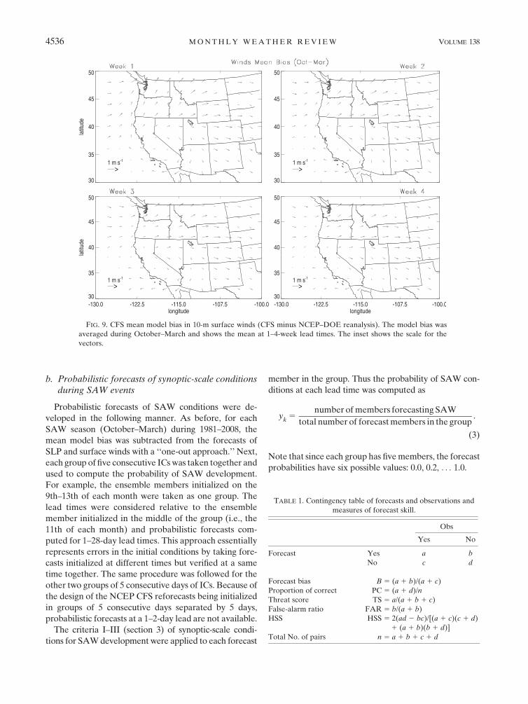
elsewhere. Likewise, the CFS model bias in the surface

zonal U and meridional V wind components were com-

puted and indicate an anticyclonic bias centered over

central California (Fig. 9). In general, the model bias in

surface winds is on the order of 1 m s21 or less. Pre-

sumably because of the small model climate drift on

short time scales, the model bias also does not change

significantly during weeks 1–4.

a. Nonprobabilistic forecasts of synoptic-scaleconditions during SAW events

Nonprobabilistic forecasts of synoptic conditions as-

sociated with SAW were evaluated by cross validation

(Wilks 2006). For each extended winter season (October–

March) during 1981–2008, the mean model bias was

subtracted from the forecasts of SLP and surface winds

with a ‘‘one out approach,’’ that is, that season was ex-

cluded from the computation of mean model bias [see

Saha et al. (2006) for additional discussion]. Next, the

forecasts of SLP and surface winds were analyzed for

each validation day during 1 October–31 March and

lead time 1–28 days. If criteria I–III (section 3) were met,

the forecast was ‘‘yes’’—synoptic-scale conditions in-

dicated SAW development at that lead time. If the

conditions were not met, the forecast was ‘‘no,’’ indicating

no conditions for SAW development. The observed re-

cords of SAW occurrences derived from NCEP–DOE

reanalysis (section 3) were used to validate the forecasts.

The total number of pairs of forecasts–observations

for each lead time of 1–28 days varied between 2430

and 2457 because the CFS reforecasts were initialized

in groups of 5 consecutive days separated by 5 days. The

pairs of forecasts–observations were aggregated into a

2 3 2 contingency table and several forecast skill mea-

sures computed [Table 1; see Wilks (2006) for details].

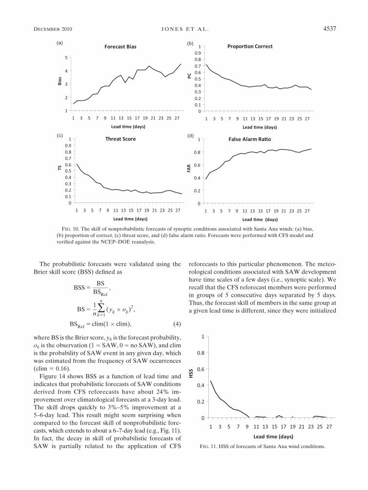
Figure 10 shows some skill score measures. The forecast

bias as a function of lead time (Fig. 10a) indicates that

nonprobabilistic forecasts derived from CFS reforecasts

tend to overforecast the synoptic conditions associated

with SAW events (unbiased forecasts have bias equal to

1). It is interesting to note that the forecast bias increases

almost linearly from 1- to 13-day lead time.

As a measure of forecast accuracy, Fig. 10b shows the

proportion of forecasts correctly indicating a maximum

of 0.71 at a 1-day lead, steadily decreasing to about 0.39

at an 11-day lead and remaining in the range of 0.34 for

long lead times. The threat score (Fig. 10c) starts from


0.60 for a 1-day lead and decreases rapidly to 0.21 at an

11-day lead time. The false alarm ratio measures the

reliability of the forecasts (Fig. 10d) and shows a value of

0.38 at a 1-day lead, increasing to 0.76 at a 9-day lead,

and then becoming nearly constant afterward.

The Heidke skill score (HSS) is a forecast skill

metric frequently used to summarize the results of

nonprobabilistic forecasts; it measures the normalized

proportion of correct forecasts after eliminating those

forecasts that would be correct just by chance (Wilks

2006). Perfect forecasts have HSS 5 1 and forecasts

with no skill have HSS 5 0. The HSS (Fig. 11) starts at

;0.45 for 1-day lead and decreases to 0 at 9-day lead

time.

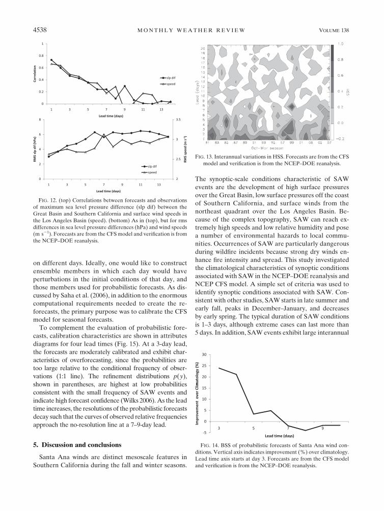
The CFS model forecast skill of SAW conditions was

further evaluated by considering two pairs of forecasts

and observations. The first one is the maximum sea level

pressure difference between the Great Basin and the

Los Angeles Basin, while the second is the surface wind

speeds in the Los Angeles Basin. Figure 12 (top) shows

correlations between forecasts and observations. The

correlations start from about 0.7 at a 1-day lead and

drop to about 0.2 at ;7-day lead time. Likewise, the

root-mean-square error between forecasts and obser-

vations (Fig. 12, bottom) indicates errors of about 3 hPa

at a 1-day lead in the maximum sea level pressure dif-

ference, increasing almost linearly to ;6 hPa at a 6-day

lead time. The errors in the surface wind speed grow

from 2.6 m s 21 at a 1-day lead to 3.1 m s21 at a 7-day

lead.

Taken together, the metrics above suggest that non-

probabilistic forecasts of synoptic-scale conditions that

lead to SAW development have some skill up to about

a 6–7-day lead time. Interannual variations in HSS were

further investigated by computing the score for each

extended winter season separately (Fig. 13). HSS $ 0.2

extends to about a 5-day lead time during most sea-

sons, while positive HSS values are still observed at a

9–12-day lead time in some seasons. The large inter-

annual variations in HSS reflect the interannual vari-

ability in the frequency of synoptic conditions associated

with Santa Ana winds. As previously discussed, ENSO

can partially explain some of the interannual variations

in SAW activity (Raphael 2003).

The results above emphasize the challenge of obtain-

ing accurate medium-to-extended range forecasts of con-

ditions conducive to dangerous wildfires in Southern

California. Additional study of high-resolution mesoscale

numerical models to provide detailed spatiotemporal

structures of SAW events is needed.

FIG. 8. CFS mean model bias in sea level pressure (hPa; CFS minus NCEP–DOE reanalysis). The model bias was

averaged during October–March and shows the mean at 1–4-week lead times. The contour interval is 0.25 hPa and

the zero line is omitted.


b. Probabilistic forecasts of synoptic-scale conditionsduring SAW events

Probabilistic forecasts of SAW conditions were de-

veloped in the following manner. As before, for each

SAW season (October–March) during 1981–2008, the

mean model bias was subtracted from the forecasts of

SLP and surface winds with a ‘‘one-out approach.’’ Next,

each group of five consecutive ICs was taken together and

used to compute the probability of SAW development.

For example, the ensemble members initialized on the

9th–13th of each month were taken as one group. The

lead times were considered relative to the ensemble

member initialized in the middle of the group (i.e., the

11th of each month) and probabilistic forecasts com-

puted for 1–28-day lead times. This approach essentially

represents errors in the initial conditions by taking fore-

casts initialized at different times but verified at a same

time together. The same procedure was followed for the

other two groups of 5 consecutive days of ICs. Because of

the design of the NCEP CFS reforecasts being initialized

in groups of 5 consecutive days separated by 5 days,

probabilistic forecasts at a 1–2-day lead are not available.

The criteria I–III (section 3) of synoptic-scale condi-

tions for SAW development were applied to each forecast

member in the group. Thus the probability of SAW con-

ditions at each lead time was computed as

yk

5number of members forecasting SAW

total number of forecast members in the group.

(3)

Note that since each group has five members, the forecast

probabilities have six possible values: 0.0, 0.2, . . . 1.0.

FIG. 9. CFS mean model bias in 10-m surface winds (CFS minus NCEP–DOE reanalysis). The model bias was

averaged during October–March and shows the mean at 1–4-week lead times. The inset shows the scale for the

vectors.

TABLE 1. Contingency table of forecasts and observations and

measures of forecast skill.

Obs

Yes No

Forecast Yes a b

No c d

Forecast bias B 5 (a 1 b)/(a 1 c)

Proportion of correct PC 5 (a 1 d)/n

Threat score TS 5 a/(a 1 b 1 c)

False-alarm ratio FAR 5 b/(a 1 b)

HSS HSS 5 2(ad 2 bc)/[(a 1 c)(c 1 d)

1 (a 1 b)(b 1 d)]

Total No. of pairs n 5 a 1 b 1 c 1 d


The probabilistic forecasts were validated using the

Brier skill score (BSS) defined as

BSS 5BS

BSRef

,

BS 51

n�

n

k51(y

k� o

k)2,

BSRef

5 clim(1� clim), (4)

where BS is the Brier score, yk is the forecast probability,

ok is the observation (1 5 SAW, 0 5 no SAW), and clim

is the probability of SAW event in any given day, which

was estimated from the frequency of SAW occurrences

(clim 5 0.16).

Figure 14 shows BSS as a function of lead time and

indicates that probabilistic forecasts of SAW conditions

derived from CFS reforecasts have about 24% im-

provement over climatological forecasts at a 3-day lead.

The skill drops quickly to 3%–5% improvement at a

5–6-day lead. This result might seem surprising when

compared to the forecast skill of nonprobabilistic fore-

casts, which extends to about a 6–7-day lead (e.g., Fig. 11).

In fact, the decay in skill of probabilistic forecasts of

SAW is partially related to the application of CFS

reforecasts to this particular phenomenon. The meteo-

rological conditions associated with SAW development

have time scales of a few days (i.e., synoptic scale). We

recall that the CFS reforecast members were performed

in groups of 5 consecutive days separated by 5 days.

Thus, the forecast skill of members in the same group at

a given lead time is different, since they were initialized

FIG. 10. The skill of nonprobabilistic forecasts of synoptic conditions associated with Santa Ana winds: (a) bias,

(b) proportion of correct, (c) threat score, and (d) false alarm ratio. Forecasts were performed with CFS model and

verified against the NCEP–DOE reanalysis.

FIG. 11. HSS of forecasts of Santa Ana wind conditions.


on different days. Ideally, one would like to construct

ensemble members in which each day would have

perturbations in the initial conditions of that day, and

those members used for probabilistic forecasts. As dis-

cussed by Saha et al. (2006), in addition to the enormous

computational requirements needed to create the re-

forecasts, the primary purpose was to calibrate the CFS

model for seasonal forecasts.

To complement the evaluation of probabilistic fore-

casts, calibration characteristics are shown in attributes

diagrams for four lead times (Fig. 15). At a 3-day lead,

the forecasts are moderately calibrated and exhibit char-

acteristics of overforecasting, since the probabilities are

too large relative to the conditional frequency of obser-

vations (1:1 line). The refinement distributions p(y),

shown in parentheses, are highest at low probabilities

consistent with the small frequency of SAW events and

indicate high forecast confidence (Wilks 2006). As the lead

time increases, the resolutions of the probabilistic forecasts

decay such that the curves of observed relative frequencies

approach the no-resolution line at a 7–9-day lead.

5. Discussion and conclusions

Santa Ana winds are distinct mesoscale features in

Southern California during the fall and winter seasons.

The synoptic-scale conditions characteristic of SAW

events are the development of high surface pressures

over the Great Basin, low surface pressures off the coast

of Southern California, and surface winds from the

northeast quadrant over the Los Angeles Basin. Be-

cause of the complex topography, SAW can reach ex-

tremely high speeds and low relative humidity and pose

a number of environmental hazards to local commu-

nities. Occurrences of SAW are particularly dangerous

during wildfire incidents because strong dry winds en-

hance fire intensity and spread. This study investigated

the climatological characteristics of synoptic conditions

associated with SAW in the NCEP–DOE reanalysis and

NCEP CFS model. A simple set of criteria was used to

identify synoptic conditions associated with SAW. Con-

sistent with other studies, SAW starts in late summer and

early fall, peaks in December–January, and decreases

by early spring. The typical duration of SAW conditions

is 1–3 days, although extreme cases can last more than

5 days. In addition, SAW events exhibit large interannual

FIG. 12. (top) Correlations between forecasts and observations

of maximum sea level pressure difference (slp dif) between the

Great Basin and Southern California and surface wind speeds in

the Los Angeles Basin (speed). (bottom) As in (top), but for rms

differences in sea level pressure differences (hPa) and wind speeds

(m s21). Forecasts are from the CFS model and verification is from

the NCEP–DOE reanalysis.

FIG. 13. Interannual variations in HSS. Forecasts are from the CFS

model and verification is from the NCEP–DOE reanalysis.

FIG. 14. BSS of probabilistic forecasts of Santa Ana wind con-

ditions. Vertical axis indicates improvement (%) over climatology.

Lead time axis starts at day 3. Forecasts are from the CFS model

and verification is from the NCEP–DOE reanalysis.


variations and possible mechanisms responsible for trends

and low-frequency variations need further study. A cli-

mate run of the CFS model showed good agreement with

the observed climatological characteristics of SAW con-

ditions and generally small differences (roughly, mean sea

level pressure differences 61 hPa and mean surface wind

differences of 1 m s21 or less), which is an encouraging

result for the prospect of forecasting such conditions.

Nonprobabilistic and probabilistic forecasts of synoptic-

scale conditions associated with SAW events were de-

rived from NCEP CFS reforecasts. The CFS model

exhibits small mean systematic biases in SLP and surface

winds in the range of a 1–4-week lead time. Several skill

measures indicate that nonprobabilistic forecasts of SAW

conditions extend to about a 6–7-day lead time. In con-

trast, probabilistic forecasts of SAW conditions show less

skill and improvements upon climatological forecasts

extend to about a 5–6-day lead. The decrease in skill

of probabilistic forecasts arises from the design of the

CFS reforecasts, in which the ensemble members were

generated by ICs in groups of 5 consecutive days sepa-

rated by 5 days. A different approach to constituting

ensemble members might be needed to produce proba-

bilistic forecasts of synoptic-scale conditions of SAW on

lead times of 2–3 weeks.

Evidently, the most important aspect of Santa Ana

winds for fire managers is the strong surface winds cou-

pled to high temperatures and low humidity, which are

highly conducive to the spread of wildfires. These mete-

orological aspects were not addressed here because of the

low spatial resolution of the NCEP–DOE reanalysis and

CFS model. The NARR dataset realistically represents

monthly frequencies of SAW occurrences (not shown)

and spatial patterns of northeasterly winds over Southern

California. The 32-km horizontal grid spacing of NARR,

however, is not able to resolve local details associated

with SAW, especially its extension over coastal waters

and formation of surface wind jets. Nevertheless, the

FIG. 15. Attributes diagrams of probabilistic forecasts of Santa Ana wind conditions at lead times of 3, 5, 7, and

9 days. Curves show observed relative frequency of Santa Ana winds conditional on I 5 6 possible probability

forecasts. Numbers in parentheses indicate relative frequency of use of forecast values, p(yi). The ‘‘.’’ symbols show

average frequencies of observations (in the vertical axis) and forecasts (horizontal axis). Solid 1:1 lines indicate

perfect calibration. Forecasts are from CFS model and verification from NCEP–DOE reanalysis.


comprehensive NARR products derived with advanced

data assimilation system can be useful to further down-

scale atmospheric conditions associated with SAW events.

High-resolution dynamical downscaling studies of SAW

currently under way will be presented in a future paper.

Acknowledgments. The North American Regional

Reanalysis was provided by the NOAA/OAR/ESRL

PSD, Boulder, Colorado, from their Web site online at

http://www.cdc.noaa.gov; their support is greatly appre-

ciated. This work is part of Cooperative Agreement 06-

JV-11272165-057 between the University of California,

Santa Barbara, and the USDA Forest Service, Pacific

Southwest Research Station in Riverside, California.

C. Jones and L. Carvalho also thank the support of NOAA

OGP Climate Test Bed (Grant NA08OAR4310698).

REFERENCES

Byram, G. M., 1959: Combustion of forest fuels. Forest Fire Control

and Use, K. P. Davis, Ed., McGraw Hill, 61–89.

Castro, R., A. Pares-Sierra, and S. G. Marinone, 2003: Evolution

and extension of the Santa Ana winds of February 2002 over

the ocean, off California and the Baja California Peninsula.

Cien. Mar., 29, 275–281.

——, A. Mascarenhas, A. Martinez-Diaz-De-Leon, R. Durazo,

and E. Gil-Silva, 2006: Spatial influence and oceanic thermal

response to Santa Ana events along the Baja California Pen-

insula. Atmosfera, 19, 195–211.

Cohen, J. D., and J. E. Deeming, 1985: The national fire-danger

rating system: Basic equations. General Tech. Rep. PSW-82,

U.S. Department of Agriculture, Forest Service, Pacific

Southwest Forest and Range Experiment Station, Berkeley,

CA, 16 pp.

Conil, S., and A. Hall, 2006: Local modes of atmospheric vari-

ability: A case study of southern California. J. Climate, 19,

4308–4325.

Corbett, S. W., 1996: Asthma exacerbations during Santa Ana

winds in southern California. Wilderness Environ. Med., 7,

304–311.

Fosberg, M. A., 1978: Weather in wildland fire management: The

fire weather index. Proc. Conf. on Sierra Nevada Meteorology,

Lake Tahoe, CA, Amer. Meteor. Soc., 1–4.

Gallus, W. A., Jr., and J. B. Klemp, 2000: Behavior of flow over step

orography. Mon. Wea. Rev., 128, 1153–1164.

Goodrick, C. L., 2002: Modification of the Fosberg fire weather

index to include drought. Int. J. Wildland Fire, 11, 205–211.

Hu, H., and W. T. Liu, 2003: Oceanic thermal and biological re-

sponses to Santa Ana winds. Geophys. Res. Lett., 30, 1596,

doi:10.1029/2003GL017208.

Hughes, M., and A. Hall, 2009: Local and synoptic mechanisms

causing Southern California’s Santa Ana winds. Climate Dyn.,

34, 847–857, doi:10.1007/s00382-009-0650-4.

Kanamaru, H., and M. Kanamitsu, 2007: Fifty-seven-year Cal-

ifornia Reanalysis Downscaling at 10 km (CaRD10). Part II:

Comparison with North American Regional Reanalysis.

J. Climate, 20, 5572–5592.

Kanamitsu, M., and H. Kanamaru, 2007: Fifty-seven-year Cal-

ifornia Reanalysis Downscaling at 10 km (CaRD10). Part I:

System detail and validation with observations. J. Climate, 20,

5553–5571.

——, W. Ebisuzaki, J. Woollen, S.-K. Yang, J. J. Hnilo, M. Fiorino,

and G. L. Potter, 2002: NCEP-DOE AMIP-II Reanalysis

(R-2). Bull. Amer. Meteor. Soc., 83, 1631–1643.

Keeley, J. E., and C. J. Fotheringham, 2001: Historic fire regime in

Southern California shrub lands. Conserv. Biol., 15, 1536–

1548.

——, ——, and M. A. Moritz, 2004: Lessons from the October 2003

wildfires in Southern California. J. For., 102, 26–31.

Lea, D. H., 1969: Some climatological aspects of Santa Ana winds

at Point Mugu. Pacific Missile Range, Point Mugu, CA, 125 pp.

Lu, R., R. P. Turco, K. Stolzenbach, S. K. Friedlander, C. Xiong,

K. Schiff, L. Tiefenthaler, and G. Wang, 2003: Dry deposition

of airborne trace metals on the Los Angeles Basin and adja-

cent coastal waters. J. Geophys. Res., 108, 4074, doi:10.1029/

2001JD001446.

Lynn, R. J., and J. Svejkovsky, 1984: Remotely sensed sea-surface

temperature variability off California during a Santa Ana

clearing. J. Geophys. Res., 89, 8151–8162.

McCutchan, M. H., and M. J. Schroeder, 1973: Classification of

meteorological patterns in Southern California by discrimi-

nant analysis. J. Appl. Meteor., 12, 571–577.

Mesinger, F., and Coauthors, 2006: North American Regional

Reanalysis. Bull. Amer. Meteor. Soc., 87, 343–360.

Miller, L. N., and N. J. Schlegel, 2006: Climate change projected

fire weather sensitivity: California Santa Ana wind occurrence.

Geophys. Res. Lett., 33, L15711, doi:10.1029/2006GL025808.

Minnich, R. A., 1987: Fire behavior in Southern California chap-

arral before fire control: The Mount Wilson burns at the turn

of the century. Ann. Assoc. Amer. Geogr., 77, 599–618.

Moritz, M. A., 2003: Spatiotemporal analysis of controls on

shrubland fire regimes: Age dependency and fire hazard.

Ecology, 84, 351–361.

Phuleria, H. C., P. M. Fine, Y. F. Zhu, and C. Sioutas, 2005: Air

quality impacts of the October 2003 Southern California wild-

fires. J. Geophys. Res., 110, D07S20, doi:10.1029/2004JD004626.

Raphael, M. N., 2003: The Santa Ana winds of California. Earth

Interactions, 7. [Available online at http://EarthInteractions.

org.]

Reheis, M. C., and R. Kihl, 1995: Dust deposition in southern

Nevada and California, 1984–1989—Relations to climate,

source area, and source lithology. J. Geophys. Res., 100, 8893–

8918.

Ryan, C. C., 1969: A vertical perspective of Santa Ana winds in

a canyon. U.S.D.A. Forest Service Research Paper PSW-52,

12 pp.

Saha, S., and Coauthors, 2006: The NCEP Climate Forecast Sys-

tem. J. Climate, 19, 3483–3517.

Schroeder, M. J., and C. C. Buck, 1970: Fire weather. U.S.D.A.

Forest Service, Agriculture Handbook, 229 pp.

——, M. Glovinsky, V. F. Henricks, F. C. Hood, and M. K. Hull,

1964: Synoptic weather types associated with critical fire

weather. Rep. 0036944, Pacific Southwest Forest and Range

Experiment Station, Berkeley, CA, 503 pp.

Small, I. J., 1995: Santa Ana Winds and the fire outbreak of fall

1993. Tech. Memo., NOAA/NWS, 48 pp.

Sosa-Avalos, R., G. Gaxiola-Castro, R. Durazo, and B. G. Mitchell,

2005: Effect of Santa Ana winds on bio-optical properties off

Baja California. Cien. Mar., 31, 339–348.

Svejkovsky, J., 1985: Santa Ana airflow observed from wildfire

smoke patterns in satellite imagery. Mon. Wea. Rev., 113,

902–906.


Taylor, S. J., R. Bright, G. Carbin, P. Bothwell, and R. Naden, 2003:

Using short range ensemble model data in national fire weather

outlooks. Extended Abstracts, Fifth Symp. on Fire and Forest

Meteorology and Second Int. Wildland Fire Ecology and Fire

Management Congress, Orlando, FL, Amer. Meteor. Soc., 2.7.

Trasvina, A., M. Ortiz-Figueroa, H. Herrera, M. A. Cosio, and

E. Gonzalez, 2003: ‘Santa Ana’ winds and upwelling fila-

ments off Northern Baja California. Dyn. Atmos. Oceans, 37,113–129.

Wang, W., S. Saha, H.-L. Pan, S. Nadiga, and G. White, 2005:

Simulation of ENSO in the new NCEP Coupled Forecast

System Model (CFS03). Mon. Wea. Rev., 133, 1574–1593.

Westerling, A. L., D. R. Cayan, T. J. Brown, B. L. Hall, and

L. G. Riddle, 2003: Climate, Santa Ana winds and autumn

wildfires in southern California. Eos, Trans. Amer. Geophys.

Union, 85, 289–300.

Whiteman, C. D., 2000: Mountain Meteorology: Fundamentals and

Applications. Oxford University Press, 355 pp.

Wilks, D. S., 2006: Statistical Methods in the Atmospheric Sciences.

2nd ed. Academic Press, Inc., 648 pp.

Wu, J., A. M. Winer, and R. J. Delfino, 2006: Exposure assessment

of particulate matter air pollution before, during, and after

the 2003 Southern California wildfires. Atmos. Environ., 40,

3333–3348.


Documents

Forecast Skill of Synoptic Conditions Associated with