HAL Id: halshs-01679456https://halshs.archives-ouvertes.fr/halshs-01679456

Preprint submitted on 9 Jan 2018

HAL is a multi-disciplinary open accessarchive for the deposit and dissemination of sci-entific research documents, whether they are pub-lished or not. The documents may come fromteaching and research institutions in France orabroad, or from public or private research centers.

L’archive ouverte pluridisciplinaire HAL, estdestinée au dépôt et à la diffusion de documentsscientifiques de niveau recherche, publiés ou non,émanant des établissements d’enseignement et derecherche français ou étrangers, des laboratoirespublics ou privés.

Forecasting and risk management in the Vietnam StockExchange

Manh Ha Nguyen, Olivier Darné

To cite this version:Manh Ha Nguyen, Olivier Darné. Forecasting and risk management in the Vietnam Stock Exchange.2018. �halshs-01679456�

EA 4272

Forecasting and risk management in the Vietnam Stock Exchange

Manh Ha Nguyen* Olivier Darné*

2018/03

(*) LEMNA - Université de Nantes

Laboratoire d’Economie et de Management Nantes-Atlantique

Université de Nantes Chemin de la Censive du Tertre – BP 52231

44322 Nantes cedex 3 – France http://www.lemna.univ-nantes.fr/

Tél. +33 (0)2 40 14 17 17 – Fax +33 (0)2 40 14 17 49

Docu

men

t de T

rava

il W

orkin

g Pa

per

1

Forecasting and risk management in the Vietnam Stock Exchange

NGUYEN Manh Ha1 2

LEMNA, University of Nantes

DARNÉ Olivier3

LEMNA, University of Nantes

Abstract

This paper analyzes volatility models and their risk forecasting abilities with the presence

of jumps for the Vietnam Stock Exchange (VSE). We apply GARCH-type models, which capture

short and long memory and the leverage effect, estimated from both raw and filtered returns.

The data sample covers two VSE indexes, the VN index and HNX index, provided by the Ho Chi

Minh City Stock Exchange (HOSE) and Hanoi Stock Exchange (HNX), respectively, during the

period 2007 - 2015. The empirical results reveal that the FIAPARCH model is the most suitable

model for the VN index and HNX index.

Keywords: Vietnam Stock exchange, volatility, GARCH models, Value-at-Risk.

JEL Classification: C22, C53, G10, G17

1 IAE Nantes, Institute of Economics and Management, Chemin de la Censive du Tertre, BP 52231, 44322 Nantes

Cedex 3, France. Phone: +33 (0)2 40 14 17 00. Fax: +33 (0)2 40 14 17 17. E-mail: manh-ha.nguyen@etu.univ-

nantes.fr.

2 Faculty of Banking and Finance, Foreign Trade University. 91 Chua Lang Street, Dong Da District, Hanoi City.

Phone: +84 (04) 32595158 (ext: 280,284). Fax: +84 (04) 38343605

3 IAE Nantes, Institute of Economics and Management, Chemin de la Censive du Tertre, BP 52231, 44322 Nantes

Cedex 3, France. Phone: +33 (0) 2 40 14 17 05. Fax: +33 (0)2 40 14 17 17. E-mail: Olivier.Darne@univ-nantes.fr.

2

1. Introduction

Together with the banking system, the stock market is an important financial source for

the economy. Conversely, changes in policies and legal instruments and the variability of

macroeconomic indicators have an impact on stock market returns and volatility. Compared to

other stock markets in the world, the Vietnamese stock exchange (VSE) is rather young. The

first trading of the Ho Chi Minh Stock Exchange (HOSE) was started on July 28, 2000 with

only two securities, and that of the Hanoi Stock Exchange (HNX) was on July 14, 2005. After

more than 10 years of operation, despite much volatility, the VSE has thrived significantly. The

number of listed companies has been considerably increased from only 2 listed companies in

July 2000 to 453 in 2009 and 694 in 2011. By the end of 2015, 684 tickers and fund

certificates had been listed on the HOSE and HNX, with a total value of USD 24.32 billion,

corresponding to an increase of 25% in comparison with 2014. In addition, the market

capitalization reached approximately USD 59.321 billion, which was equivalent to 30.7% of

the GDP of the country. However, the average daily trading volume is quite small,

approximately USD 113.04 million.4

During the financial crisis of 2007-2009, world stock markets witnessed a fall in their

asset price and exhibited volatility. The VSE had also experienced several difficulties, and the

bubble burst. Both the VN index (HOSE) and the HNX index (HNX) declined by nearly 70%

in 2008, one of the biggest loss ever seen in any of the world stock markets. Since 2009, the

VSE has been still unstable, with high volatility. In this context, an empirical study on the

volatility of the VSE is required.

Volatility in the equity market, which is a fundamental concept in the discipline of finance,

has been seen as a measure of the uncertainty of investment’s rate of return. As a proxy of risk,

modeling and forecasting stock market volatility have become a concerned subject of numerous

4 Note that the HOSE and HNX exchanges are categorized as frontier market country (i.e., non-investible markets) by the Financial Times and the London Stock Exchange (FTSE).

3

empirical and theoretical contributions over past decades. Forecasting and modeling stock

volatility are crucial inputs for pricing derivatives and for trading and hedging strategies.

Furthermore, the extreme volatility could disrupt the smooth functioning of the financial system

and lead to structural or regulatory changes. Therefore, it is important to understand the behavior

of return volatility. Autoregressive Conditional Heteroskedasticity (ARCH) introduced by

Engle (1982), independently extended to the Generalized ARCH (GARCH) model by

Bollerslev (1986) and Taylor (1986), and improved GARCH-type models have been developed

to capture the most important stylized facts of stock returns, which are heavy-tailed distributed,

volatility clustering, leverage effect and long memory volatility. To examine the characteristics

of VSE return volatility, this paper uses 10 members of GARCH family models, namely,

GARCH, EGARCH, GJR-GARCH, IGARCH, RiskMetrics, APARCH, FIGARCH,

FIAPARCH, FIEGARCH and HYGARCH models.

However, it is well known that stock markets are subject to some drastic shocks, called

large shocks, outliers or jumps (references). This type of event includes, for example, oil

shocks, wars, financial slumps, changes of policy regimes, and natural disasters. These shocks

may have undesirable effects on the tests of conditional homoscedasticity (e.g., van Dijk et al.,

1999; Carnero et al., 2007), the identification and estimation of GARCH models governing the

conditional volatility of returns, and thus on the out-of-sample volatility forecasts (e.g., Franses

and Ghijsels, 1999; Carnero et al., 2007, 2012; Charles, 2008) and Value-at-Risk predictions

(e.g., Mancini and Trojani, 2011; Iqbal and Mukherjee, 2012; Dupuis et al., 2015). In this paper,

we thus address jumps in two ways. First, we detect jumps in the VSE returns from the additive

jump detection procedure in GARCH models proposed by Franses and Ghijsels (1999), and

then apply GARCH-type models on the filtered returns. Then, we use the back-testing of Kupiec

(1995) and Engle and Manganelli (2004) to compare the predictive ability of models estimated

from the original and adjusted-outlier returns in terms of forecasting market, in particular from

Value-at-Risk (VaR).

4

The paper is organized as follows. The literature review is given in Section 2. Section 3

describes the Vietnam stock exchange. Section 4 presents the methodology and provides data

information. The empirical results are discussed in Section 5. Section 6 analyzes the VaR and

back-testing. Section 7 provides some concluding comments.

2. Literature review

This section pays special attention to the empirical studies relating to Vietnam's young

stock market. One of the first studies developed by Vuong (2004) finds evidence of GARCH

effects on return series of ten listed companies and the VN index during the period of 2000-

2003. In another study, Farber et al. (2006) show that the HOSE presents an anomaly of stock

returns and a strong herd effect by using the daily stock return from 2000 to 2006. The authors

also argue that the ARMA-GARCH model is the best one in the case of serial correlations and

fat-tailed for the stabilized period. However, Do et al. (2009) use GARCH(1,1) and GJR-

GARCH(1,1) to characterize the returns and volatility of ASEAN emerging stock markets

(Indonesia, Malaysia, the Philippines, Thailand and Vietnam), incorporating with the effects

from the international gold market. The GJR-GARCH(1,1) model seems to be effective in

describing daily stock returns’ features for most of these stock markets, except Vietnam.

However, as the exogenous variables (the one-day-lagged returns and the one-day-lagged return

volatility in the PM London Gold Fix) are introduced, GARCH(1,1)-X captures better stock

market volatility behavior than the GJR-GARCH(1,1)-X, except for Indonesia. Daily closing

data of the stock market indexes and the PM London Gold Fix were selected in the period from

July 28, 2000 to October 31, 2008.

More recently, Truong (2012), employing the OLS and GARCH (1,1) model for daily

return of HNX index series from 2002 to 2011, evidences the day-of-the-week effects on stock

returns and the presence of volatility in the HNX market. Similarly, Le et al. (2012) evaluate

5

the day-of-the-week of eight stock market indexes from both developed and developing

countries including Vietnam over the period 2002-2008 through a broad set of econometric

models, notably GARCH, modified GARCH (daily dummies added into the conditional

variance equation of standard GARCH), modified GARCH-M, modified TGARCH and

modified EGARCH models. Similar to Truong (2012), the authors note a negative Tuesday

return in the case of Vietnam, which is reliably documented in eight models.

The GARCH family models have also been applied to examine the effects of external

shocks on the VSE. For instance, Chang et al. (2009) adopt a non-linear threshold model with

the bivariate Momentum Threshold Error-Correction Model- Glosten, Jagannathan and Runkle

GARCH (MTECM-GJR-GARCH(1,1)) process to consider the asymmetric return and

volatility transmission relationships between exchange rate and stock prices in Vietnam. Daily

closing values of Vietnamese stock price and exchange rates are collected from Datastream for

the period from July 28, 2000 to December 29, 2006, a total of 1,416 observations. The leverage

effect is evidenced in both the Vietnam exchange rate and stock markets. Then, they are a strong

interaction between the stock price and exchange rate. The empirical results indicate that

Vietnam stock prices will revert to the long-term equilibrium level when a disequilibrium term

created by changes to the exchange rate market. Using the same model, Chang and Su (2010)

find that the development of Japan and Singapore stock markets influences the VSE. Moreover,

they confirm the existence of asymmetric volatility effect in the VSE. In contrast, Tran (2011)

suggests that the effects of shocks on volatility were symmetric in the VSE. The author also

explores the relevance of GARCH models in explaining stock return dynamics and volatility

on the Vietnamese stock market during the period January - October 2009. Luu (2011) uses

ARMA-GARCH and ARMA-EGARCH models to examine the relationship between the US

and the VSE. The research analyzes 1,483 daily observations from 2003-2009. The author finds

evidence that the S&P500 index has a positive and strong significant influence on the VN index

return. However, there is no evidence of volatility spillover effects between the two indexes.

6

Moreover, several recent studies focus on the effect of macroeconomic factors on the

VSE. For instance, Vo and Batten (2010) investigate the relationship between liquidity and

stock returns in the VSE during the financial crisis period by using a data set ranging from 2006

to 2010. They reveal that liquidity positively affected stock returns. In another work, Vo (2016)

suggests that institutional investors stabilized the stock return volatility in the HOSE for the

period 2006–2012. Finally, according to Vo and Nguyen (2011), GARCH and GARCH-in-

mean (GARCH-M) models are the appropriate models in describing daily stock returns’

features. The data employed in this study comprise 2,121 observations of daily closing stock

price index of the HOSE, obtained from March 01, 2002 to August 31, 2010. Regarding

structural breaks, the number of volatility shifts significantly decreases in comparison with the

raw return series when applying ICSS to standardized residuals filtered from the GARCH (1,1)

model.

Furthermore, some other authors have adopted the Value-at-Risk model (VaR) to

determine and predict the level of risk when investing in the VSE. More recently, Vo et al.

(2010), employing the GARCH and the VaR model for daily return of VN index series from

2000 to 2010, evidences the GARCH effects on stock returns and the presence of a weak-form

efficient market in the HOSE. The authors also argue that the IGARCH model is the best one

to determine VaR. Similarly, Hoang et al. (2011) confirm that the daily return of the VN index

in the period from July 28, 2000 to March 31, 2011 can be captured by the GARCH (1,1) model.

In particular, through the VaR model on the VN index, GARCH forecasts fairly accurately the

risk of capital loss of the portfolio, thus supporting investors in making reasonable decisions on

fund allocation. Meanwhile, Hoang et al. (2015) have adopted the model GARCH-EVT

(Extreme Value Theory)-Copula, normal distribution and empirical distribution to estimate the

VaR (Value at Risk) and ES (Expected Shortfall) of some shares listed on the Vietnamese stock

market. The study used data from January 02, 2007 to December 28, 2012 and comprised 11

series of stock returns. Back-testing VaR and ES results showed that the conditional Copula

7

method and EVT are appropriate and reflect the actual value of losses on the portfolio more

precisely than yield stocks with a normal distribution.

3. Overview of the Vietnam stock exchange

Vietnam has made significant progress in the transition from a centrally planned economy

to a market-oriented system. Political and economic reforms (Đổi Mới) launched in 1986 have

transformed the country from one of the poorest in the world, with GDP per capita (current

USD) of approximately USD 143, to lower middle income status within a quarter of a century

with approximately USD 2,100 by the end of 2015. Vietnam’s economy continued to strengthen

in 2015, with an estimated GDP growth rate of 6.86% for the entire year.

Together with the positive changes in the economic situation, the financial background in

Vietnam has also changed significantly. Capital market development has also been considered

an important factor that facilitates the ongoing banking sector reforms. Established in 1990,

Vietnam’s banking industry has grown tremendously from a mono-banking system to a huge

network of banks and financial institutions. Over the past 25 years, the Vietnamese government

has initiated many banking reforms for decades to improve the efficiency and competitiveness

of the banking system in the country, in particular through the privatization of its state-owned

banks. By 2015, Vietnam’s banking sector comprised 7 state-owned commercial banks

(SOCBs), 28 joint stock banks (JSBs), 50 foreign bank branches, 3 joint venture banks, 5 banks

with 100% foreign capital and two development and policy banks.

Moreover, reforming State-owned enterprises (SOEs) is the biggest concern in Vietnam.

The government plans to undertake reforms through equalization and subsequent initial public

offerings (IPOs), which are expected to improve the SOEs efficiency and productivity. The

SOE reforms undertaken by the Government has resulted in the development of capital markets.

8

Consequently, the Government established the State Securities Commission (SSC) in 1997 and

set the necessary legal framework.

As a result of these changes, two stock markets, the HOSE and HNX, have been

established. The Ho Chi Minh City Securities Trading Center (HOSTC), which was established

in July 28, 2000, became the HOSE on August 8, 2007. The HOSE is currently the largest stock

exchange in Vietnam, which is the market for big corporations with capital greater than USD

5.51 million. The second securities trading center, the Hanoi Securities Trading Center

(HASTC), opened in March 2005 and is oriented for small and medium companies with capital

from USD 0.688 million. In January 2009, according to a decision of the Prime Minister of

Vietnam, the HASTC was renamed and restructured as the Hanoi Stock Exchange (HNX).

The first transaction of the HOSE started on July 28, 2000 with only two listed companies,

notably the Saigon Cable and Telecommunication Material Joint Stock Company (SAM) and

Refrigeration Electrical Engineering Joint Stock Company (REE), with a total market

capitalization of USD 30,600. The VSE experienced very slow growth during the beginning

period. By the end of 2000, there were only 5 stockholding companies listed with market

capitalization accounting for 0.2% GDP in 2000. From 2001 to 2004, there were only 26

stockholding listed companies with total capital of USD 0.269 billion. Total market

capitalization just reached 0.54% of GDP in 2004. In 2005, there was an optimistic outlook for

the securities market. By the end of 2005, there were 38 shareholdings listed companies on the

HOSTC and HASTC, which were mainly restructured SOEs through equalization. The total of

market capitalization reached USD 0.583 billion in 2005, contributing 1.01% of GDP. In

general, before 2006, the VSE was operated in a tentative manner.

9

Figure 1: The number of listed companies on the HOSE and HNX during 2000-2015

Source: Author’s estimation from HOSE and HNX Annual Reports for 2000 - 2015

With some encouraging policies and positive responses from domestic and international

investors, 2006 was considered a boom year for the VSE with 151 newly listed companies.

Since 2006, the VSE has become very active in terms of quantity and quality. By the end of

2006, there were 193 listed companies on the HOSE and HNX. Total stocks circulated in the

markets increased 8 times compared to the entire previous period of 2000 - 2005. The total

market capitalization by the end of 2006 reached USD 13.776 billion (equivalent to 20.76% of

GDP), 20 times higher than that in 2005.

Following the success of 2006, in 2007, the Vietnam government made a set of promoting

measures for its stock markets, including promoting the equalization of SOEs and implement

the Law on Securities. Consequently, on March 12, 2007, the VN index (HOSE) reached a

record height of 1,170.67 points. Similarly, the HNX index had ending at 242.89 points

(+146.65 points), increasing by 153.37% compared to 2006. The total market capitalization had

a record of USD 30.690 billion (equivalent to 39.64% of GDP).

0

50

100

150

200

250

300

350

400

450

2000 2001 2002 2003 2004 2005 2006 2007 2008 2009 2010 2011 2012 2013 2014 2015

HOSE HNX

10

Influenced by the global economic crisis, the year of 2008 was a volatile and disastrous

one for the VSE. Record inflation and a large trade deficit led to a macro-financial imbalance.

In this context, the Government tightened its monetary policy and domestic banks reduced their

capital into stock markets. The market capitalization plunged with a loss of approximately USD

16 billion. The 2008 turmoil caused an end to eight years of gains on the HOSE and three years

of gains on the HNX. Both the VN and the HNX indexes declined by nearly 70% in 2008, one

of the biggest losses ever seen in any world stock market. The HNX index even fell below its

starting point of 100 in November 2008.

The year of 2009 was marked by the arrival of three biggest ex-SOE companies on the

HOSE, notably, the Vietnam Insurance Corporation (Bao Viet), Bank for Foreign Trade of

Vietnam (Vietcombank), and Industrial and Commercial Bank of Vietnam (Vietinbank). The

total value of market capitalization reached over USD 34.578 billion (32.62% of GDP). By the

end of 2010, with 642 joint-stock companies, Vietnam’s total market capitalization reached

USD 38.2 billion. Since 2012, VSE has borne many negative impacts of macroeconomic

instability such as high inflation and that of the liquidity of the banking system. For instance,

market capitalization decreased significantly, reaching only USD 25.785 billion, dropping

25.7% compared to that by the end of 2010, accounting for 19.02% of GDP. Moreover, as

displayed in Figure 2, in comparison with other countries in the region, the market

capitalization/GDP ratio of the VSE is the lowest.

11

Figure 2: Market capitalization/GDP (%) of ASEAN’s countries

Source: Author’s calculation from WDI’s data and HOS and, HNX Annual Reports in 2011

While most regional equity markets recovered quickly after the 2007 financial crisis,

Vietnam has not yet reached its record level again. The market capitalization in 2012 gained

only 24% of GDP. Furthermore, the number of newly listed companies on the HNX has dropped

significantly from 104 in 2010 to 14 in 2012.

Currently, although the world economy still contains many uncertainties, Vietnam’s

economy has recovered fairly. For instance, after reaching the peak of 18.68% in 2011,

Vietnam’s inflation rate has fallen into single digits since 2012 and has steadily decreased in

the following years, as reported in Table 1. In this period, following the recovery of economic

activities, market capitalization has also grown steadily. In this context, more private investors

have engaged in the stock markets, and the stock market has been playing an increasingly more

important role in Vietnam’s economy.

19.020

72.445

217.379

132.781

43.686

73.643

0.000

50.000

100.000

150.000

200.000

250.000

Vietnam Thailand Singapore Malaysia Indonesia Philippines

12

Table 1: The growth of GDP and CPI of Vietnam over 2010-2015

2010 2011 2012 2013 2014 2015

GDP growth (annual %) 6.42 6.24 5.25 5.42 5.98 6.68

Inflation, consumer prices

(annual %)

8.86 18.68 9.09 6.59 4.09 0.63

Source: Author’s calculation from WDI’s data

The world economy in 2015 experienced many up and down trends such as the plunge of

China’s economy and stock market, exchange rate issues, the movement of international capital

flows, and plummeting oil prices. However, Vietnam’s stock markets in 2015 remained

relatively stable and were considered a bright spot for attracting foreign capital inflows relative

to other regional countries. In 2015, the GDP of Vietnam grew by 6.68%, outperforming the

previous figure of 5.98% in 2014 and achieving the peak for the last 5 years. Similarly, inflation

in 2015 slightly increased by 0.63%, recorded as the lowest rate over the last 15 years. As result,

the stock market in 2015 closed with the VN Index reaching 579.03 points, up 5.5% over the

beginning of the year but it still fell short of investors’ expectations. Market capitalization raised

through the stock market hit USD 139.599 billion, accounting for 30.64% of GDP. Furthermore,

the quantity of listed companies had increased from 642 listed companies in 2010 to 684

companies in 2015 to diversify goods in the stock market.

13

Figure 3: Market capitalization of the VSE over 2000-2015

Source: Author’s calculation from HOSE and HNX Annual Reports during 2000 – 2015

Since its establishment in July 2000, Vietnam’s stock market has strengthened and

expanded the financial system, as it serves trade, hedge, and diversify and pool risks. It has

become a critical channel in terms of producing an efficient allocation of capital, and short and

long-term investments, which contribute to the expansion of business operations, and has

become more diversified and effective for an overall domestic economy. The stock market has

assumed a developmental role in global economics and the financial system of Vietnam.

0.000

10.000

20.000

30.000

40.000

50.000

60.000

70.000

2000 2001 2002 2003 2004 2005 2006 2007 2008 2009 2010 2011 2012 2013 2014 2015

market capitalization (billion USD) market capitalization (% of GDP)

14

Figure 4: The comparison between Vietnam’s GDP growth and Market capitalization

during 2000-2015

Source: Author’s calculation from WDI’s data, and HOSE and HNX Annual Reports during

2000 - 2015

Stock market activity also plays an important role in determining the level of economic

development. As seen in Figure 4, there is a relative co-movement in the relationship between

Vietnam’s economic growth and market capitalization. Vietnam achieved an approximate 8%

in annual GDP growth from 1990 to 1997, and it continued at approximately 7% from 2000 to

2005. Continuously, Vietnam had the record of having GDP growth at 6.98% and 7.13% in

2006 and 2007, and experienced an inflation rate of 7.39% and 8.30%, respectively. Vietnam

is becoming the world's second-fastest growing economy, following China only. This is also a

booming period for the Vietnamese stock market with growth in listed companies (250) and

market capitalization (39.64%). Due to the deeper integration into the world's economy,

Vietnam has been heavily influenced by the 2007 financial crisis. Vietnam's economic growth

had fallen to 5.66%, and its inflation had reached a record of 23.12%. These events mark a

0

5

10

15

20

25

30

35

40

45

0.00

1.00

2.00

3.00

4.00

5.00

6.00

7.00

8.00

2000200120022003200420052006200720082009201020112012201320142015

GDP growth (annual %) Market capitalization (% of GDP)

15

significant decrease in the VSE’s activities. As the economy has become stable since 2012, the

stock market has also grown steadily.

Figure 5: Structure of Vietnam’s GDP by sector during 1990-2015

Source: Author’s calculation from WDI’s data

We now turn to the composition of the VSE. As shown in Figure 5, during the early years

of economic reforms, agriculture played a key role in the national economy. The contribution

of the agricultural sector to GDP was 32.94% during the period 1990-1995. This figure steadily

decreased during the following five-year periods (1996-2000), 25.85%, 22.32%, 20.89% and

18.95%, respectively. In the context of industrializing and modernizing Vietnam’s economy,

industry and the services sector have played an increasingly decisive role in economic growth.

Particularly from 2001, the service sector has gradually set its position in an increasing

32.9425.854 22.318 20.89 18.952

26.7133.106 39.566 41.36

36.726

40.35 41.04 38.116 37.75

40.308

0.00

20.00

40.00

60.00

80.00

100.00

120.00

1990-1995 1996-2000 2001-2005 2006-2010 2011-2015

Agriculture, value added (% of GDP) Industry, value added (% of GDP)

Services, etc., value added (% of GDP)

16

contribution through each stage. This is also illustrated by an increasing number of listed

companies on the VSE. The listed companies are mainly concentrated in the financial sector

and industrial areas, with the percentages 41.16% and 34.36%, respectively, in 2009. Since

2014, the financial sector has retained its leading position (24.5%), followed by consumer

staples (21.8%), and utilities (15.2%). On January 25, 2015, the HOSE officially announced the

Sectoral Index of Global Industry Classification Standard GICS®5, in which the financial sector

has retained its first place (41.47%), followed by consumer staples (21.05%), and utilities

(12.24%) on the HOSE. Similarly, on the HNX, the financial and industrial sectors have taken

the first and second positions with 35.06% and 17.11%, respectively, followed by the oil and

gas mining sector with 12.42%, and the construction sector with 12.02%.

5 MSCI and Standard & Poor’s developed the Global Industry Classification Standard (GICS), seeking to offer an efficient investment tool to capture the breadth, depth and evolution of industry sectors. It consists of 10 sectors, 24 industry groups, 67 industries and 156 sub-industries

17

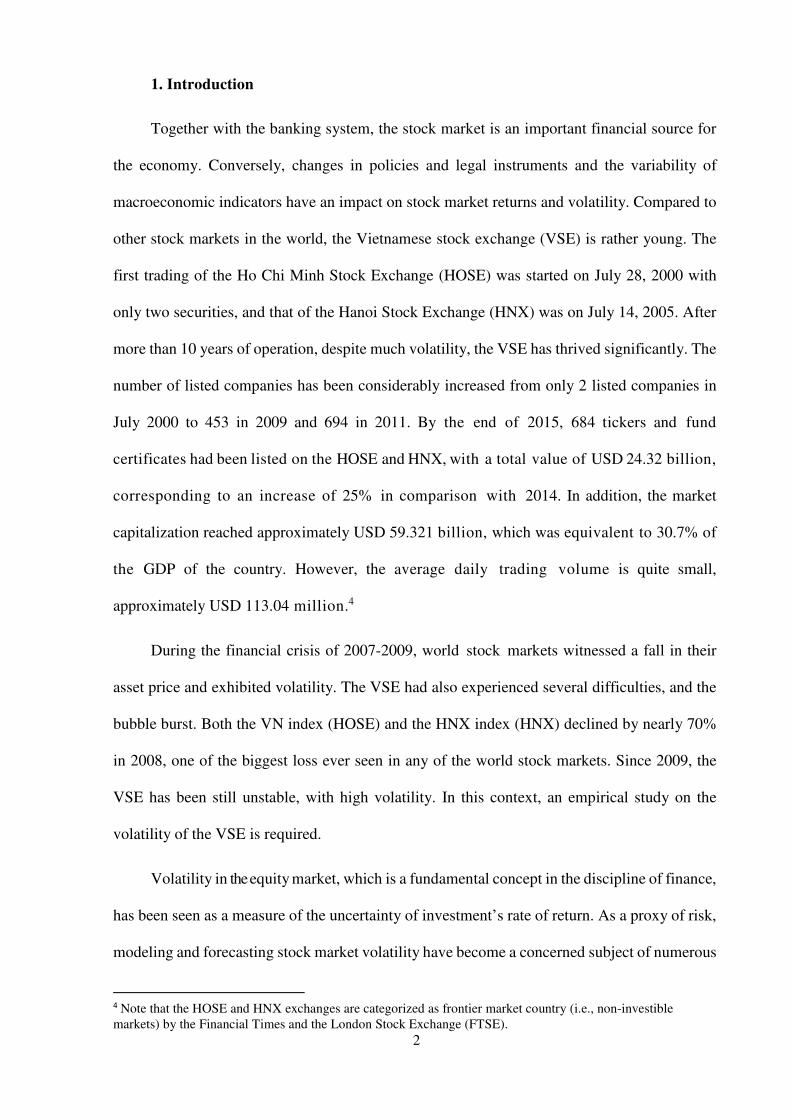
Figure 6: Structure of listed value by sector on the HOSE and HNX, 2016

Source: Author’s calculation from HOSE’s data and HNX’s data

After 16 years of operation, the development of the VSE has also been explained by the

contribution of both domestic and foreign investors. Foreign investors’ activities in the stock

market have been still prudentially controlled. In 2003, foreign ownership in listed companies

was limited up to 30% of company capital. However, since September 2005, the Government

has expanded the limitation of foreign securities in investor ownership from 30% up to 49%

(except companies in the banking field). Compared to Decree 58/2012, Decree 60/2015

abandoned the limit of the ownership percentage of foreign investors. Accordingly, except for

HOSE HNX

2% 1%5%

7%

41%9%

21%

2%

12%

Health Care Energy

Consumer Discretionary Materials

Financial Industrials

Consumer Staples Information Technology

Utilities

1%

12%

10%

12%

35%

17%

6%

1%

5%

1%

Health CareMining, Oil and GasTrade and accommodation services, mealsConstructFinancialIndustrialsReal estateScience and technology; administrative and support servicesTransportation and storageInformation, communications and other activities

18

the international commitments of Vietnam as integration and business conditions, the

proportion of foreign ownership is unrestricted in public companies, unless stated in company

rules.

Figure 7: The number of foreign investors in the VSE during 2006-2015

Source: Author’s calculation from the VSD’s data

Before 2005, the role of foreign investors was not featured in the Vietnamese stock

market. Since 2006, foreign investors have participated quite actively in the market. In 2006,

there were 3,050 individuals and 239 organizations with trading codes. By the end of 2015, the

Vietnamese Stock Depository (VSD) had granted stock transactions code for 18,607 foreign

investors, including 2,879 organizations and 15,728 individual investors, increasing 99.65%

and 17.43%, respectively, compared to those in 2010.

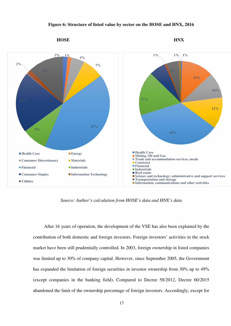
Moreover, the amount of capital transactions by foreign investors in the VSE has been

increasing significantly. In 2009, foreign investors purchased nearly 70.26 million shares and

sold approximately 65.56 million shares. Foreign investors have focused on purchasing blue-

chips stocks with high market value and selling stocks with low value. The net buying value of

foreign investors reached its record of USD 805.68 million in 2010. In general, foreign

investors’ participation has increased market liquidity for transactions worth approximately

0

2000

4000

6000

8000

10000

12000

14000

16000

18000

2006 2007 2008 2009 2010 2011 2012 2013 2014 2015

Individuals Organizations

19

26.32% of the total market trading, which could result in better and more efficient capital

allocation. Additionally, foreign investors’ participation has contributed to making corporate

governance more transparent and closer to international practices and thus to promoting the

image of Vietnam's economy.

Figure 8: The comparison of transaction value of foreign investors and the overall

market trading

Source: Author’s calculation from the HOSE’s data

4. Overview on GARCH models

4.1. The GARCH model

Autoregressive conditionally heteroscedastic (ARCH) models introduced by Engle

(1982), extended to GARCH models, independently, by Bollerslev (1986) and Taylor (1986),

have become important tools in the analysis of time series data, particularly in financial

applications to analyze and forecast volatility. They have been proved to be sufficient in

capturing the most important stylized facts of stock return, which are time-varying volatility,

heavy-tailed distribution, volatility clustering and volatility persistence.

One weaknesses of the ARCH model is that it requires too many parameters and a high

order q to capture the volatility process. To reduce this limitation, Bollerslev (1986) and Taylor

15.3

19.61

35.99

28.3131.99

25.1427.92

0

5

10

15

20

25

30

35

40

2009 2010 2011 2012 2013 2014 2015

Buy Sell Buy + Sell

20

(1986) independently proposed the Generalized ARCH (GARCH) model. The GARCH model,

which is an extension of the ARCH model, not only keeps all the characteristics of the ARCH

model but also reduces the number of estimated parameters by imposing nonlinear restrictions.

The GARCH model has been raised with a new term, the lagged conditional variance term

(����� ). An unexpected increase or decrease in returns at time t will generate an increase in the

expected variability in the next period. The standard GARCH (1,1) can be given by:

r� = μ + ε� = μ+σ�z�, ~NID(0,1) (1)

where �� is the daily return at time t computed as �� = ln(��/����) x 100, with �� ������� the

stock prices at time t and (t-1), µ is the conditional mean of the asset return r�, ε� = σ��� is the

prediction error, σ� > 0 is the conditional standard deviation of the underlying asset return

(denoted volatility) and the standardized error �� ∼ NID(0, 1).

��� = ! + "#���� + $����� (2)

A sufficient condition of the GARCH(1, 1) model for the conditional variance to be

positive is ω > 0, α > 0, β ≥ 0.6 The stationary of the process is achieved when the restriction α

+ β < 1 is satisfied. Ling and McAleer (2002a, 2002b) have derived the regularity conditions of

a GARCH(1,1) model, defined as follows: %&#��' = (��)�* < ∞ if α + β < 1 and %&#�-' < ∞

6 Nelson and Cao (1992) show that the restrictions imposed by Bollerslev (1986), i.e., the non-negativity of all parameters in

the condition variance specification, can be substantially relaxed. They derive necessary and sufficient conditions for the GARCH(1,1) model. More specifically, some of the parameters are allowed to have a negative sign. Note that the Nelson and Cao (1992) conditions are implemented in econometric packages such as G@RCH package for Ox.

21

if ."� + 2"$ + $� <1, where k is the conditional fourth moment of ��.7 Ng and McAleer (2004)

show the importance to verify these conditions.

The sum of α and β quantifies the persistence of shocks to conditional variance, meaning that

the effect of a volatility shock vanishes over time at an exponential rate. The GARCH models

are short-term memory, which define explicitly an intertemporal causal dependence based on a

past time path. In such a model, the probability of a price increasing or decreasing is a function

of both the current state of the price but also the prices assumed in the previous instants.

Another linear GARCH-class model is the IGARCH model of Engle and Bollerslev

(1986), which can capture infinite persistence in the conditional variance. It means that a shock

of variance in the current conditions will have an impact on the predicted values in the future.

The model setting of the IGARCH(1,1) model is similar to that of GARCH(1,1), but the

coefficients α and β satisfy the condition that α + β = 1. This parameter restriction is imposed

when estimating the conditional variance specification. The unconditional variance of an

IGARCH model is not finite, implying the complete persistence of such a shock, that is, multi-

period forecasts of volatility will tend upwards. The IGARCH(1,1) can be written as:

��� = ! + "#���� + (1 − ")����� (3)

Additionally, The RiskMetrics volatility specification of JP Morgan is also a special case

of the IGARCH and GARCH models, where the autoregressive parameter is set at a pre-

specified value of 0.94 and the coefficient of #���� , is equal to 0.06. It is widely used to forecast

7 Under the assumption of Normal distribution, k = 3, and thus, the condition becomes 3"� + 2"$ + $� <1. See Ling and

McAleer (2002a, 2002b) for other distributions.

22

short term variations and is defined as:

��� = 0.06#���� + 0.94����� (4)

The GARCH model possesses many advantages, but it also has some limitations in

estimating the volatility. First, GARCH is symmetric and does not measure the asymmetric

leverage effect, where increases in volatility are larger when previous returns are negative than

when they have the same magnitude but are positive. Indeed, GARCH equally evaluated good

and bad information in the stock market. The asymmetric volatility property is explained in the

literature in terms of the leverage effect and the volatility feedback effect. The leverage

hypothesis (Black, 1976; Christie, 1982; Schwert, 1989) suggests that bad news (negative return

shocks) increases financial leverage and makes the stocks riskier, which in turn increases

market volatility. The volatility feedback hypothesis relies on the widely documented finding

of volatility persistence (see Bollerslev et al., 1992) and time-varying risk premiums (see

French et al., 1987; Campbell and Hentchel, 1992). As the volatility feedback story goes, bad

news brings higher current stock volatility, which induces market participants to revise upward

the conditional variance since volatility is persistent. Increased conditional variance leads to an

instantaneous decline in market price so that investors can be compensated in the form of

additional expected return. Thus, in the case of bad news, the volatility feedback effect further

strengthens the leverage effect. Second, the constraint of non-negative parameters involves the

conditional variance, which is not negative. Thus, a shock, no matter what its sign is, always

has a positive effect on the volatility. To solve these drawbacks, the GARCH model has been

further improved. To capture the asymmetric leverage volatility effect, a new class of GARCH

models was introduced with the asymmetric (non-linear) GARCH models, such as the GJR-

GARCH model by Glosten, Jagannathan and Runkel (1993), the exponential GARCH

23

(EGARCH) model by Nelson (1991), and the asymmetric power ARCH (APARCH) model by

Ding et al. (1993).

4.2. The asymmetric GARCH models

The GJR model developed by Glosten et al. (1993) is constructed to capture the potential

larger impact of negative shocks on return volatility. The specification for the conditional

variance of GJR-GARCH(1,1) model is:

��� = ! + "#���� + 67���#���� + $����� (5)

where 7���is an indicator variable taking value one if the residual (#�) is smaller than zero and

the value zero if the residual (#�) is not smaller than zero. The coefficient 6 captures the

asymmetric effect of a negative shock on the conditional variance as opposed to a positive

shock. γ > 0, is the asymmetric leverage coefficient, which describes the volatility leverage

effect. The volatility is positive if α > 0, γ ≥ 0, α + γ ≥ 0 and β ≥ 0. The process is defined as

stationary if the constraint α + β + (γ/2) < 1 is satisfied. Ling and McAleer (2002b) have derived

the regularity conditions for a GJR-GARCH(1,1), defined as follows: %&#��' < ∞ if α + β + γδ

<1 and %&#�-' < ∞ if k"� + 2"$ +$� + $6 + ."6 + .96� < 1.8 The GJR-GARCH model

nets the GARCH model when γ = 0.

Another popular nonlinear GARCH-class model, which can also depict the volatility

leverage effect, is the Exponential GARCH (EGARCH) one proposed by Nelson (1991). As

8 Under a Normal distribution and a Student-t(v) distribution, with v > 5, 9 = �� . See Ling and McAleer (2002a, 2002b) for

other distributions.

24

opposed to GJR-GARCH, the conditional variance of the EGARCH is always positive even if

the parameter values are negative; thus, there is no need for parameter restrictions to impose

non-negativity. The EGARCH(1,1) model is given as:

log(���) = ! +>�?��� + >�(|?���| − E|?���|) + $log(����� ) (6)

where >�B|��| − %(|#�|)Cdetermines the size effect and the term >��� define the sign effect of

the shocks on volatility, with �� is the standardized residual. The specification of the volatility

in terms of its logarithmic transformation implies that the parameters in this model are not

restricted to positive values. β measures the persistence in conditional volatility irrespective of

anything occurring in the market. According to Alexander (2009), volatility will take a long

time to die out following a crisis in the market when β is relatively large. Furthermore, a

sufficient condition for the stationarity of the EGARCH model is |$| < 1. The θ parameter

measures the asymmetry or the leverage effect, the parameter of importance, so that the

EGARCH model allows for the testing of asymmetries. If >� = 0, then the model is symmetric.

If >� < 0, positive shocks (good news) will create less volatility than negative ones, and this

impact is vice versa when >� > 0.

Another variant of the asymmetric GARCH model is the asymmetric power ARCH

(APARCH) model of Ding et al. (1993). The APARCH model is defined as:

��D= ! + "(|#���| − 6#���)D+ $����D (7)

25

where ! > 0, α ≥ 0 and β ≥ 0. The parameter 9 (9 > 0) plays the role of a Box-Cox

transformation of the conditional standard deviation �� while 6 reflects the so-called leverage

effect, with -1 < γ < 1. Furthermore, the condition for the existence of %(��D) is given by ακ +

β < 1, where κ = %(|#� − 1| − 6#���)D, which depends on the error distribution. Ding et al.

(1993) derive the expression of κ for Gaussian errors, and Lambert and Laurent (2001) and

Karanasos and Kim (2006) obtain it for Skewed-Student and Student distributions, respectively.

The APARCH model includes several GARCH extensions as special cases, including the

GARCH(1,1) model when 9 = 2 and 6 = 0, and the GJR-GARCH (1,1) one when 9 = 2.

4.3. The long-memory GARCH models

A GARCH model features an exponential decay in the autocorrelation of conditional

variances. However, it has been noted that squared and absolute returns of financial assets

typically have serial correlations that are slow to decay similar to those of an I(d) process. A

shock in the volatility series seems to have very long memory and impact on future volatility

over a long horizon. The IGARCH model captures this effect but a shock in this model has an

impact upon future volatility over an infinite horizon, and the unconditional variance does not

exist for this model. This model implies that shocks to the conditional variance persist

indefinitely, and this is difficult to reconcile with the persistence observed after large shocks,

such as the crash of October 1987, as well as with the perceived behavior of agents who do not

appear to frequently and radically alter the composition of their portfolios, as would be implied

by IGARCH (Mills, 1990). Thus, the widespread observation of the IGARCH behavior may be

an artifact of a long memory.

If the IGARCH model assumes that the impact of shocks on the conditional variance does

not dissipate over time but continues infinitely, the fractionally integrated GARCH

(FIGARCH) model of Baillie et al. (1996) encompasses the possibility of persistent but not

26

necessarily permanent shocks to volatility, in which the conditional variance at time t is an

infinite moving average of the squared realizations of the series up to time t−1. The FIGARCH

(1,d,1) model can be written as:

��� = ! + &1 − (1 − $G)��((1 − ∅G)(1 − G)I'#�� (8)

where 0 ≤ d ≤ 1, ω > 0, ϕ and β < 1, and d is the fractional integration parameter while L is the

lag operator. Conrad and Haag (2006) have derived necessary and sufficient conditions for the

non-negativity of the conditional variance in the FIGARCH (1,d,1) model.

The degree of hyperbolic decay in the long-memory property is governed by the

parameter d, which allows autocorrelations to decay at a slow hyperbolic rate. One advantage

of the FIGARCH model is that it can describe three different situations in which reflect the

impacts of lagged squared innovations on the conditional variance: (1) the intermediate ranges

of persistence given by 0 < d < 1, implying a long-memory behavior and a slow rate of decay

after a volatility shock; (2) the complete integrated persistence of volatility shocks associated

with d = 1 (IGARCH model); and (3) the geometric decay associated with d = 0 (GARCH

model).

Davidson (2004) proposed another long-memory model of the conditional variance, the

hyperbolic GARCH (HYGARCH) model, a special case of GARCH and FIGARCH, with

success in modeling the long-run dynamics in the conditional variance of several financial time

series. While sharing the desired properties of the covariance stationarity with GARCH model,

the HYGARCH one still obeys hyperbolically decaying impulse response coefficients, as does

27

the FIGARCH model.9 It can be viewed as a two-component GARCH specification with one

component being GARCH and the other being FIGARCH. The HYGARCH (1,d,1) model is

defined as follows:

��� = ! + {1 − (1 − $G)��∅G&1 + .(1 − G)I − 1'}#�� (9)

where 0 ≤ d ≤1, ω > 0, k ≥ 0, φ, β > 1 and L is the lag operator. The HYGARCH model nests

the FIGARCH and GARCH models when k = 1 and 0, respectively. For 0 < k < 1 this process

is stationary, while for k > 1, it implies that this process is non-stationary. Conrad (2010) has

derived non-negativity conditions for the HYGARCH (1,d,1) model that are necessary and

sufficient.

4.4. The asymmetric and long-memory GARCH models

The FIGARCH (p,d,q) model explained earlier the persistence, fat-tailed and volatility

clustering in the series. One limit of this model is the variance structure depends only on the

sign of innovations t, which is contrary to the empirical behavior of stock market prices, which

allows for the leverage effect. To accommodate for asymmetries between positive and negative

shocks, Bollerslev and Mikkelsen (1996) extend the FIGARCH process to FIEGARCH, to

correspond with Nelson’s (1991) EGARCH model to allow for asymmetry. Thus, this model

accounts for long memory in volatility (fractional integration, as in the FIGARCH model of

Baillie et al. (1996)) and asymmetric volatility reaction to positive and negative return

9 The HYGARCH model permits the existence of second moments at more extreme amplitudes compared with the simple IGARCH and FIGARCH models. Thus, the HYGARCH model is covariance stationary while the IGARCH and FIGARCH models are not covariance stationary.

28

innovations (the exponential feature, as in Nelson's (1991) EGARCH model). The

FIEGARCH(1,d,1) model is given as:

ln(���) = ω + (1 − G)I"M(����) + $Nn(����� )

g(��) = >�(|��| − %(|��|)) + >��� (10)

Note that the functional form for g(��) accommodates the asymmetric relationship

between stock returns and volatility changes associated with the leverage effect by both a “sign

effect”, >���, and a “size effect”, >�(|��| − %(|��|)). %(|��|)depends on the assumption made

on the unconditional density of��,with �� is the standardized residual. For Normal distribution

%(|��|) = O2/P. Same as the EGARCH model, this model does not impose any positivity

restrictions on the coefficients of the volatility (α, β, >�and >�). The FIEGARCH (1,d,1)

specification nests the conventional EGARCH model for d = 0.

Finally, the fourth class of GARCH model is associated with the combined stylized

features of long memory and asymmetric volatility. Tse (1998) developed the fractionally

integrated asymmetric power ARCH (FIAPARCH) model, through the expansion of the

APARCH model to a process that is fractionally integrated such as the FIGARCH specification,

and the FIGARCH process modification to allow for asymmetry. The FIAPARCH (1,d,1)

model can then be written as follows:

��� = ! + &1 − (1 − $G)��(1 − ∅G)(1 − G)I'(|#�| − 6#�)D (11)

where 0 ≤ d ≤ 1, ω and δ > 0, ϕ and β < 1, and −1 < γ < 1. The FIAPARCH process is therefore

reduced to the FIGARCH one when γ = 0 and δ = 2.

29

4.5. Outlier data in GARCH model

Excess kurtosis and volatility clustering are some important parameters to determine

high-frequency time series of returns on financial assets. The common method to access this

pattern is the GARCH model, which is used to model these two stylized facts and forecast their

volatility. The GARCH model, however, still remains a problem about excess kurtosis (Baillie

and Bollerslev, 1989) in the residuals standardized by the conditional volatility. An alternative

study is to address the outliers in returns series, which give better solutions, while the GARCH

model cannot fulfill it (Balke and Fomby, 1994; Fiorentini and Maravall, 1996). There are some

undesirable effects on the identification and the estimation of GARCH models governing the

conditional volatility of returns (e.g., Franses and Ghijsels, 1999; Carnero et al., 2007, 2012,

2016; Charles, 2008; Raziq et al., 2017).

A number of procedures have been developed to identify these outliers on linear models

(e.g., Tsay, 1986; Chang et al., 1988; Chen and Liu, 1993). Nevertheless, it is well known that

the world is not linear, and neither are financial data. There are several methods for detecting

outliers in a nonlinear setting (Hotta and Tsay, 1999; Sakata and White, 1998; Franses and

Ghijsels, 1999; Franses and van Dijk, 2000; Charles and Darné, 2005; Doornik and Ooms,

2005, Zhang and King, 2005; Grané and Veiga, 2014) based on intervention analysis as

originally proposed by Box and Tiao (1975). Here, we use the method proposed by Franses and

Ghijsels (1999) to detect and correct additive outliers (AOs) when using GARCH models.

Consider the return series ��, which is defined in Eq. (1), and the conditional volatility

follows a GARCH(1,1) model given by:

��� = ! + "#���� + $����� (12)

30

The GARCH(1,1) model can be rewritten as an ARMA(1,1) model for #��

#�� = ω + (α + β)#���� + T� − βT��� (13)

where T� =#�� - ��. The additive outliers (AO) can be modeled by regression polynomials as

follows:

U�� =#�� + !ξ(W)7�(X) (14)

where 7�(X) is the indicator function defined as 7�(X) = 1 if t = τ, and zero otherwise, with τ the

date of outlier occurring, ω and Y(W) denote the mangnitude and the dynamic pattern of the

outlier effect, respectively, with Y(W) = 1.

An AO is related to an exogenous change that directly affects the series and only its level

of the given observation at time t = τ. We can write Eq. (14) as

T� = �Z��[\ + P(W)#�� (15)

Similarly, the observed residuals �� are given by

�� = �Z��[\ + P(W)U�� =T� + P(W)!ξ(W)7�(X) (16)

Expression (17) can be interpreted as a regression model for ��, i.e.,

�� = ω]� +T� (17)

with ]� = 0, and t<τ, ]� = 1 f and t=τ, ]^_` = −P`.

Detection of outliers is based on the following statistic:

31

X̂(X) = ((b(^)cbd )(∑ ]��f�g^ )�/� = ((∑ ]�h�f�g^ )/�ij)(∑ ]��f�g^ )��/� (18)

where �ij� denotes the estimated variance of the residual process.

5. Data description

In this paper, we use the VN index of the HOSE and the HNX index of the HNX to capture

the main characteristics of the VSE. Moreover, to increase the persuasiveness of our study, we

use the FTSE Vietnam Index as another alternative market indicator.

The VN and HNX indexes are composite indexes calculated from prices of all common

stocks traded on the official Vietnam stock exchange. Specifically, the VN index is a market

capitalization weighted price index, which compares the current market value of all listed

common shares to the value on the base date of July 28, 2000 - the first traded session on the

market. Similar to the VN index, the HNX index has been calculated since July 14, 2005. The

VN and HNX indexes were initially set at 100 points.

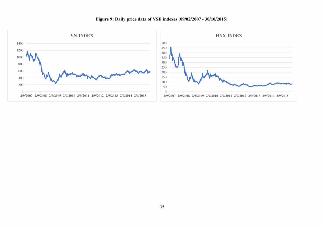
In this paper, we collect the daily data from Thomson Datastream. We use 2,266

observations for the two stock exchanges of Vietnam over the period from February 09, 2007

to October 15, 2015. Figure 9 and 10 display the prices and returns of VSE indexes.

32

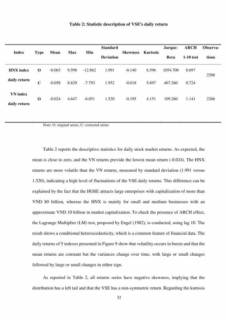
Table 2: Statistic description of VSE’s daily return

Note: O: original series, C: corrected series

Table 2 reports the descriptive statistics for daily stock market returns. As expected, the

mean is close to zero, and the VN returns provide the lowest mean return (-0.024). The HNX

returns are more volatile than the VN returns, measured by standard deviation (1.991 versus

1.520), indicating a high level of fluctuations of the VSE daily returns. This difference can be

explained by the fact that the HOSE attracts large enterprises with capitalization of more than

VND 80 billion, whereas the HNX is mainly for small and medium businesses with an

approximate VND 10 billion in market capitalization. To check the presence of ARCH effect,

the Lagrange Multiplier (LM) test, proposed by Engel (1982), is conducted, using lag 10. The

result shows a conditional heteroscedasticity, which is a common feature of financial data. The

daily returns of 5 indexes presented in Figure 9 show that volatility occurs in bursts and that the

mean returns are constant but the variances change over time, with large or small changes

followed by large or small changes in either sign.

As reported in Table 2, all returns series have negative skewness, implying that the

distribution has a left tail and that the VSE has a non-symmetric return. Regarding the kurtosis

Index Type Mean Max Min Standard

Deviation Skewness Kurtosis

Jarque-

Bera

ARCH

1-10 test

Observa-

tions

HNX index

daily return

O -0.063 9.598 -12.862 1.991 -0.140 6.596 1054.700 0.697 2266

C -0.058 8.829 -7.793 1.952 -0.018 5.697 407.260 0.724

VN index

daily return O -0.024 4.647 -6.051 1.520 -0.195 4.151 109.260 1.141 2266

33

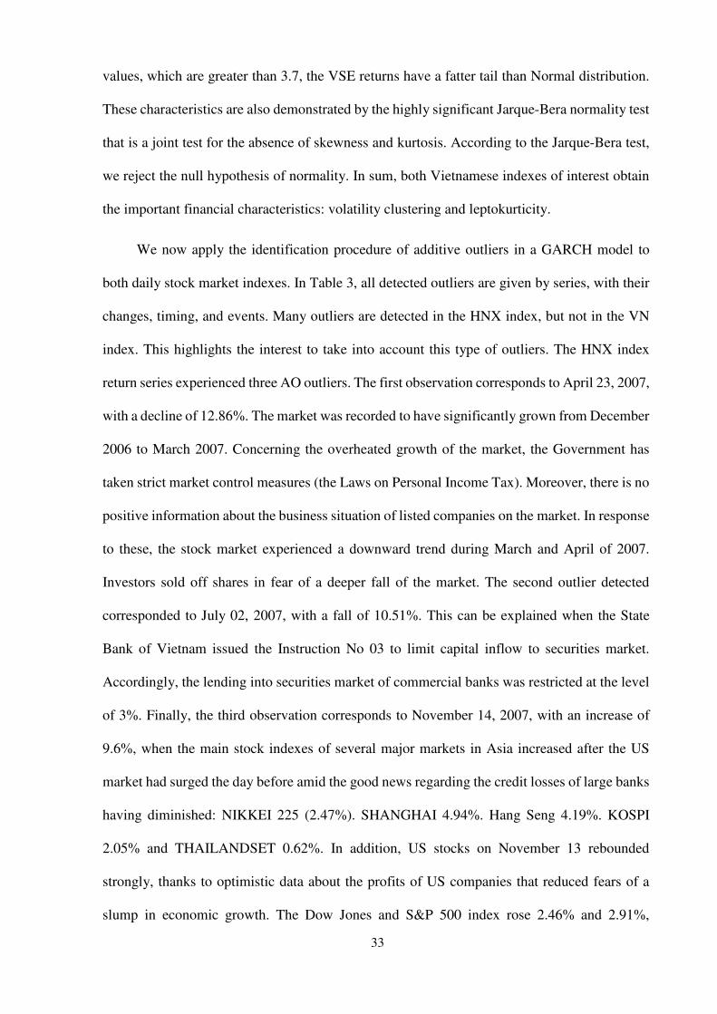
values, which are greater than 3.7, the VSE returns have a fatter tail than Normal distribution.

These characteristics are also demonstrated by the highly significant Jarque-Bera normality test

that is a joint test for the absence of skewness and kurtosis. According to the Jarque-Bera test,

we reject the null hypothesis of normality. In sum, both Vietnamese indexes of interest obtain

the important financial characteristics: volatility clustering and leptokurticity.

We now apply the identification procedure of additive outliers in a GARCH model to

both daily stock market indexes. In Table 3, all detected outliers are given by series, with their

changes, timing, and events. Many outliers are detected in the HNX index, but not in the VN

index. This highlights the interest to take into account this type of outliers. The HNX index

return series experienced three AO outliers. The first observation corresponds to April 23, 2007,

with a decline of 12.86%. The market was recorded to have significantly grown from December

2006 to March 2007. Concerning the overheated growth of the market, the Government has

taken strict market control measures (the Laws on Personal Income Tax). Moreover, there is no

positive information about the business situation of listed companies on the market. In response

to these, the stock market experienced a downward trend during March and April of 2007.

Investors sold off shares in fear of a deeper fall of the market. The second outlier detected

corresponded to July 02, 2007, with a fall of 10.51%. This can be explained when the State

Bank of Vietnam issued the Instruction No 03 to limit capital inflow to securities market.

Accordingly, the lending into securities market of commercial banks was restricted at the level

of 3%. Finally, the third observation corresponds to November 14, 2007, with an increase of

9.6%, when the main stock indexes of several major markets in Asia increased after the US

market had surged the day before amid the good news regarding the credit losses of large banks

having diminished: NIKKEI 225 (2.47%). SHANGHAI 4.94%. Hang Seng 4.19%. KOSPI

2.05% and THAILANDSET 0.62%. In addition, US stocks on November 13 rebounded

strongly, thanks to optimistic data about the profits of US companies that reduced fears of a

slump in economic growth. The Dow Jones and S&P 500 index rose 2.46% and 2.91%,

34

respectively, and the NASDAQ index rose 89.52 points (up 3.46%). In addition, oil prices fell

below $92 per barrel, which also boosted the stock market.

After applying the outlier detection method, we observed that the coefficient of skewness

of the HNX index decreased and was still negative. As result, the presence of asymmetry in

those returns was rejected. Additionally, the excess kurtosis remained significant for all series

but the values are less important than the original series. The coefficients of skewness and

kurtosis along with the Jarque-Bera (JB) test support the view that the distribution of series is

not Normal and in particular seems leptokurtic and volatility clustering, coinciding with the

empirical findings of the original return series. Finally, the outlier-filtered returns also exhibit

conditional heteroscedasticity.

Overall, the descriptive statistics suggest that an appropriate model of VSE return

volatility should account for its time-varying nature and the non-Normality of VSE returns, as

do the GARCH-type models.

Table 3: Outliers in volatility of VSE

Series Date Changes Events

HNX-index 23/04/2007 -12.86% Fearing the decline of the strong market, investors withdrew the

capital

02/07/2007 -10.51% Instruction No 3 of State Bank, limited capital inflow of

securities market.

14/11/2007 9.6% US stocks on November 13 rebounded strongly, and the main

stock indexes of several major markets in Asia increased.

35

Figure 9: Daily price data of VSE indexes (09/02/2007 - 30/10/2015)

0

200

400

600

800

1000

1200

1400

2/9/2007 2/9/2008 2/9/2009 2/9/2010 2/9/2011 2/9/2012 2/9/2013 2/9/2014 2/9/2015

VN-INDEX

0

50

100

150

200

250

300

350

400

450

500

2/9/2007 2/9/2008 2/9/2009 2/9/2010 2/9/2011 2/9/2012 2/9/2013 2/9/2014 2/9/2015

HNX-INDEX

36

Figure 10: Daily return of VSE (09/02/2007 - 30/10/2015)

-0.08

-0.06

-0.04

-0.02

0

0.02

0.04

0.06

2/9/2007 2/9/2008 2/9/2009 2/9/2010 2/9/2011 2/9/2012 2/9/2013 2/9/2014 2/9/2015

VN-index daily return

-0.15

-0.1

-0.05

0

0.05

0.1

0.15

2/9/2007 2/9/2008 2/9/2009 2/9/2010 2/9/2011 2/9/2012 2/9/2013 2/9/2014 2/9/2015

HNX-index daily return

37

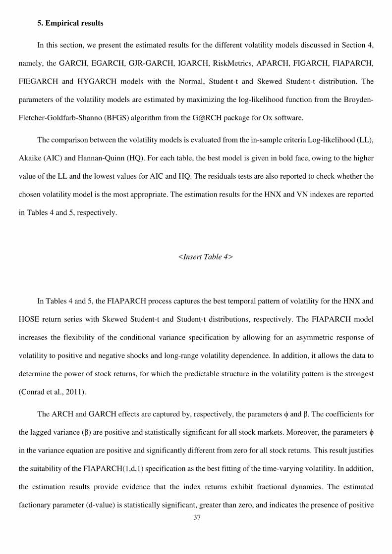
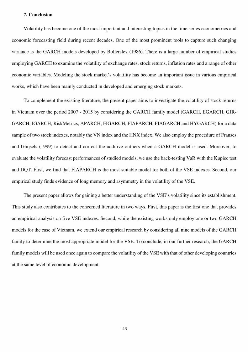
5. Empirical results

In this section, we present the estimated results for the different volatility models discussed in Section 4,

namely, the GARCH, EGARCH, GJR-GARCH, IGARCH, RiskMetrics, APARCH, FIGARCH, FIAPARCH,

FIEGARCH and HYGARCH models with the Normal, Student-t and Skewed Student-t distribution. The

parameters of the volatility models are estimated by maximizing the log-likelihood function from the Broyden-

Fletcher-Goldfarb-Shanno (BFGS) algorithm from the G@RCH package for Ox software.

The comparison between the volatility models is evaluated from the in-sample criteria Log-likelihood (LL),

Akaike (AIC) and Hannan-Quinn (HQ). For each table, the best model is given in bold face, owing to the higher

value of the LL and the lowest values for AIC and HQ. The residuals tests are also reported to check whether the

chosen volatility model is the most appropriate. The estimation results for the HNX and VN indexes are reported

in Tables 4 and 5, respectively.

<Insert Table 4>

In Tables 4 and 5, the FIAPARCH process captures the best temporal pattern of volatility for the HNX and

HOSE return series with Skewed Student-t and Student-t distributions, respectively. The FIAPARCH model

increases the flexibility of the conditional variance specification by allowing for an asymmetric response of

volatility to positive and negative shocks and long-range volatility dependence. In addition, it allows the data to

determine the power of stock returns, for which the predictable structure in the volatility pattern is the strongest

(Conrad et al., 2011).

The ARCH and GARCH effects are captured by, respectively, the parameters ϕ and β. The coefficients for

the lagged variance (β) are positive and statistically significant for all stock markets. Moreover, the parameters ϕ

in the variance equation are positive and significantly different from zero for all stock returns. This result justifies

the suitability of the FIAPARCH(1,d,1) specification as the best fitting of the time-varying volatility. In addition,

the estimation results provide evidence that the index returns exhibit fractional dynamics. The estimated

factionary parameter (d-value) is statistically significant, greater than zero, and indicates the presence of positive

38

persistence phenomenon in the index series volatility. Thus, the volatility displays the long memory or long-range

dependence property. The results show that the HOSE returns seem to have a lower degree of long-memory

behavior than the HNX returns (d = 0.455 and 0.644, respectively). Moreover, the power term δ (HNX: 2.023,

HOSE: 1.719) of stock returns for the predictable structure in the volatility pattern is positive and statistically

significant for all stock markets. In addition, the estimates for the asymmetric parameter γ are positive and

statistically significant for all stock market returns, confirming the assumption of the asymmetric effect. Indeed,

a positive value of γ means that past negative shocks have a more severe impact on current conditional volatility

than past positive shocks. That is, negative shocks give rise to higher volatility than positive shocks. Note that

the HOSE index exhibits a higher degree of asymmetry than the HNX index (HNX: 0.108, HOSE: 0.139).

In addition, the degree of asymmetry can be calculated by the formula |kl�km|kl_km for the EGARCH model and

(α+γ)/α for the GJR-GARCH model. With the EGARCH model, the results show that the degree of asymmetry

of the VN return is larger than that of the HNX return, 1.328 versus 1.255. Moreover, we also obtain the same

results with the GJR-GARCH. In particular, the degree of asymmetry of the HNX return is 1.547, while that of

the VN return is 1.584.

Panel B of Table 4 shows that the better specification of the HNX index is the FIGARCH model with a

Student distribution when the data are cleaned of outliers. This result shows that the asymmetric effect disappears

when outliers are taken into account, suggesting that the presence of outliers can bias the identification and

estimation of asymmetric GARCH-type models, as found by Carnero et al. (2016).

<Insert Table 5>

These results indicate that the asymmetric effect is present in the markets as earlier suggested by Chang et

al. (2009). However, in the case of emerging stock markets such as Vietnam, due to the lack of professionalism,

investors buy and sell under the impact of herd mentality. As a result, the bad news quickly spreads and rather

than good news, deeply influences the market.

39

6. Value-at-Risk

During the last decade, Value-at-Risk (commonly known as VaR) has become one of the most popular

techniques to measure financial risk. The VaR method aims to capture the market risk of an asset portfolio. It

measures the maximum potential loss of a given portfolio over a prescribed holding period at a given confidence

level, which is typically chosen between 1% and 5%. Therefore, after investigating the volatility of the VSE

through a GARCH analysis, we apply the VaR technique to forecast the VSE risk level.

In mathematical terms, the VaR on day t at level α for a sample of returns is defined as the corresponding

empirical quantile at α%:

��:��~o(p, ��)

" = ��(�� < q�r)) (19)

where �� is the daily return at time t, and Pr is the probability.

Back-testing is a statistical procedure, in which actual profits and losses are systematically compared to

corresponding VaR estimates. Initially, to assess the accuracy of the model-based VaR estimates, Kupiec (1995)

provided a likelihood ratio test (LR) for testing whether the failure rate of the model is statistically equal to the

expected one (unconditional coverage). Consider that o =∑ 7�s�g� is the number of exceptions in the sample size

T:

7� = t 1, uv�� <q�r�0,uv�� >q�r�

40

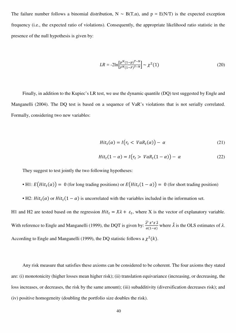
The failure number follows a binomial distribution, N ∼ B(T,α), and p = E(N/T) is the expected exception

frequency (i.e., the expected ratio of violations). Consequently, the appropriate likelihood ratio statistic in the

presence of the null hypothesis is given by:

Gr = -2lnwxy(��x)z{y|y(��|)z{y}~~�(1) (20)

Finally, in addition to the Kupiec’s LR test, we use the dynamic quantile (DQ) test suggested by Engle and

Manganelli (2004). The DQ test is based on a sequence of VaR’s violations that is not serially correlated.

Formally, considering two new variables:

�u��(") = 7B�� <q�r�(")C − " (21)

�u��(1 − ") = 7B�� >q�r�(1 − ")C − " (22)

They suggest to test jointly the two following hypotheses:

• H1: %B�u��(")C = 0(for long trading positions) or %B�u��(1 − ")C = 0 (for short trading position)

• H2: �u��(") or �u��(1 − ") is uncorrelated with the variables included in the information set.

H1 and H2 are tested based on the regression �u�� = �� +#�, where X is the vector of explanatory variable.

With reference to Engle and Manganelli (1999), the DQT is given by: ��������)(��)) where ��is the OLS estimates of �.

According to Engle and Manganelli (1999), the DQ statistic follows a ~�(.).

Any risk measure that satisfies these axioms can be considered to be coherent. The four axioms they stated

are: (i) monotonicity (higher losses mean higher risk); (ii) translation equivariance (increasing, or decreasing, the

loss increases, or decreases, the risk by the same amount); (iii) subadditivity (diversification decreases risk); and

(iv) positive homogeneity (doubling the portfolio size doubles the risk).

41

VaR fails to meet the subadditivity axiom and therefore is criticized for not being a coherent risk measure.

However, Expected Shortfall (ESF) or Conditional Value at Risk (CVaR) can be mentioned as a risk measure

that overcomes these weaknesses and has become increasingly used. ESF is an alternative to VaR that is more

sensitive to the shape of the loss distribution in the tail of the distribution. Expected Shortfall is a coherent, and

moreover a spectral, measure of financial portfolio risk. It requires a quantile-level q and is defined to be the

expected loss of portfolio value given that a loss is occurring at or below the q-quantile. ES is the conditional

expectation of the return given that it exceeds the VaR.

Let X be a continuous random variable representing loss. Given a parameter 0 < α < 1, the α-CVaR of X

is:

�q�r)(�) = %&�|� ≥ q�r)(�)' (23)

Tables 6 and 7 report our empirical results of the VaR at 1% and 5%, respectively, and the Kupiec and DQ

back-testing tests. Back-testing VaR is also employed to validate the forecast performances of volatility models.

The selected estimation and evaluation periods for each index are similar to the ones used in the out-of-sample

forecast evaluation procedure. We apply the prediction performance of the VaR to the selected GARCH-class

specifications by computing the out-of-sample forecasts. As mentioned above, the out-of-sample time series of

the VN index and HNX index cover the period from January 2, 2012 to October 19, 2015, including 991 daily

observations. A 5% VaR for each index is calculated and examined with ESF, Kupiec and DQ tests to evaluate

the volatility forecast performances of studied models.

Regarding the 5% VaR results reported in Table 6, we find that most of selected models perform well. This

result provides strong evidence that the GARCH-class models are able to capture the major stylized facts of

Vietnam’s stock market return and volatility dynamics.

With reference to DQ and Kupiec tests, we find that the FIAPARCH specifications with Skewed Student-t

distributed (or Student-t distributions) innovations provide better forecasts for all the critical levels. Specifically,

the p-values corresponding to the Kupiec LR test and the DQ test statistics are greater for all selected stock

42

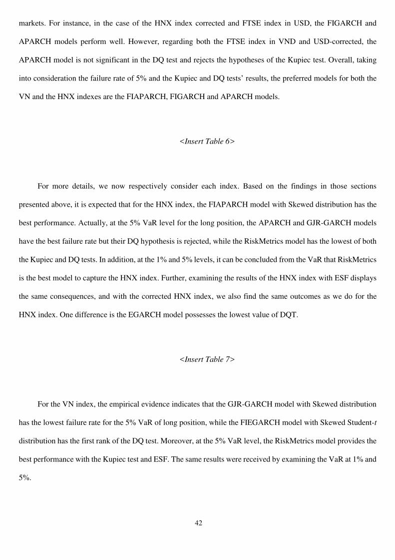
markets. For instance, in the case of the HNX index corrected and FTSE index in USD, the FIGARCH and

APARCH models perform well. However, regarding both the FTSE index in VND and USD-corrected, the

APARCH model is not significant in the DQ test and rejects the hypotheses of the Kupiec test. Overall, taking

into consideration the failure rate of 5% and the Kupiec and DQ tests’ results, the preferred models for both the

VN and the HNX indexes are the FIAPARCH, FIGARCH and APARCH models.

<Insert Table 6>

For more details, we now respectively consider each index. Based on the findings in those sections

presented above, it is expected that for the HNX index, the FIAPARCH model with Skewed distribution has the

best performance. Actually, at the 5% VaR level for the long position, the APARCH and GJR-GARCH models

have the best failure rate but their DQ hypothesis is rejected, while the RiskMetrics model has the lowest of both

the Kupiec and DQ tests. In addition, at the 1% and 5% levels, it can be concluded from the VaR that RiskMetrics

is the best model to capture the HNX index. Further, examining the results of the HNX index with ESF displays

the same consequences, and with the corrected HNX index, we also find the same outcomes as we do for the

HNX index. One difference is the EGARCH model possesses the lowest value of DQT.

<Insert Table 7>

For the VN index, the empirical evidence indicates that the GJR-GARCH model with Skewed distribution

has the lowest failure rate for the 5% VaR of long position, while the FIEGARCH model with Skewed Student-t

distribution has the first rank of the DQ test. Moreover, at the 5% VaR level, the RiskMetrics model provides the

best performance with the Kupiec test and ESF. The same results were received by examining the VaR at 1% and

5%.

43

7. Conclusion

Volatility has become one of the most important and interesting topics in the time series econometrics and

economic forecasting field during recent decades. One of the most prominent tools to capture such changing

variance is the GARCH models developed by Bollerslev (1986). There is a large number of empirical studies

employing GARCH to examine the volatility of exchange rates, stock returns, inflation rates and a range of other

economic variables. Modeling the stock market’s volatility has become an important issue in various empirical

works, which have been mainly conducted in developed and emerging stock markets.

To complement the existing literature, the present paper aims to investigate the volatility of stock returns

in Vietnam over the period 2007 - 2015 by considering the GARCH family model (GARCH, EGARCH, GJR-

GARCH, IGARCH, RiskMetrics, APARCH, FIGARCH, FIAPARCH, FIAGARCH and HYGARCH) for a data

sample of two stock indexes, notably the VN index and the HNX index. We also employ the procedure of Franses

and Ghijsels (1999) to detect and correct the additive outliers when a GARCH model is used. Moreover, to

evaluate the volatility forecast performances of studied models, we use the back-testing VaR with the Kupiec test

and DQT. First, we find that FIAPARCH is the most suitable model for both of the VSE indexes. Second, our

empirical study finds evidence of long memory and asymmetry in the volatility of the VSE.

The present paper allows for gaining a better understanding of the VSE’s volatility since its establishment.

This study also contributes to the concerned literature in two ways. First, this paper is the first one that provides

an empirical analysis on five VSE indexes. Second, while the existing works only employ one or two GARCH

models for the case of Vietnam, we extend our empirical research by considering all nine models of the GARCH

family to determine the most appropriate model for the VSE. To conclude, in our further research, the GARCH

family models will be used once again to compare the volatility of the VSE with that of other developing countries

at the same level of economic development.

44

References

1. Abed R.E, Zouheir Mighri, Z., Maktouf, S., 2016. Empirical analysis of asymmetries and long memory

among international stock market returns: A Multivariate FIAPARCH-DCC approach. Journal of Statistical and

Econometric Methods, 5 (1), 1-28.

2. Ali, S.O., Mhmoud, A.S., 2013. Estimating Stock Returns Volatility of Khartoum Stock Exchange

through GARCH Models, Journal of American Science, 9(11), 132-144.

3. Aloui C., Hamida, H.B., 2014. Modelling and forecasting value at risk and expected shortfall for GCC

stock markets: Do long memory, structural breaks, asymmetry, and fat-tails matter?, North American Journal of

Economics and Finance, 29, 349-380.

4. Angelidis, T., Benos, A., Degiannakis, S., 2004. The use of GARCH models in VaR estimation,

Statistical Methodology, 1, 105–128.

5. Awartani, B.M.A., Corradi, V., 2005. Predicting the volatility of the S&P-500 stock index via GARCH

models: The role of asymmetries. International Journal of Forecasting, 21, 167-183.

6. Baillie, R.T., Bollerslev T., Mikkelsen H.O., 1996. Fractionally integrated generalized autoregressive

conditional heteroscedasticity. Journal of Econometrics, 74, 3-30.

7. Baillie, R. T., Han, Y. W., Myers, R. J., Song, J., 2007. Long memory models for daily and high

frequency commodity futures returns. The Journal of Futures Markets, 27, 643-668.

8. Baillie, R.T., DeGennaro, R.P, 1990. Stock Returns and Volatility. Journal of Financial & Quantitative

Analysis, 25(2), 203-214.

9. Baillie, R.T., G. Geoffrey Booth G.G., Tse Y., Zabotina, T., 2002. Price discovery and common factor

models. Journal of Financial Markets, 5, 309–321.

10. Bollerslev T., Mikkelsen H.O., 1996. Modeling and pricing long memory in stock market volatility.

Journal of Econometrics, 73, 151-184.

11. Brailsford T.J., Faff R.W., 1996. An evaluation of volatility forecasting techniques. Journal of Banking

& Finance, 20, 419-438.

12. Chang H. L., Su C. W, Lai Y. C., 2009. Asymmetric Price Transmissions between the Exchange Rate

and Stock Market in Vietnam. International Research Journal of Finance and Economics, 23. 1450-2887.

45

13. Carnero, M.A., Peña, D., Ruiz, E., 2007. Effects of outliers on the identification and estimation of the

GARCH models. Journal of Time Series Analysis, 28, 471-497.

14. Carnero, M.A., Peña, D., Ruiz, E., 2012. Estimating GARCH volatility in the presence of outliers.

Economics Letters, 114, 86-90.

15. Carnero, M.A., Perez, A., Ruiz, E., 2016. Identification of asymmetric conditional heteroscedasticity

in the presence of outliers. SERIEs, 7, 179-201.

16. Charles, A., 2008. Forecasting Volatility with Outliers in GARCH model. Journal of Forecasting, 27,

551-565.

17. Charles, A., Darné. O., 2005. Outliers and GARCH Models in Financial Data. Economics Letters, 86,

347-352.

18. Cheong, C.W, 2009. Modeling and forecasting crude oil markets using ARCH-type models. Energy

Policy, 37, 2346–2355.

19. Chkili, W., Aloui, C., Nguyen D.K., 2012. Asymmetric effects and long memory in dynamic volatility

relationships between stock returns and exchange rates. Journal of International Financial Markets, Institutions

and Money, 22(4), 738-757.

20. Christoffersen, P., Pelletier, D., 2003. Backtesting Value-at-Risk: A Duration-Based Approach.

Journal of Financial Econometrics, 2 (1), 84-108.

21. Conrad, C., Karanasos, M., Zeng, N., 2011. Multivariate fractionally integrated APARCH modeling

of stock market volatility: A multi-country study. Journal of Empirical Finance, 18, 147–159.

22. Dimson, E., Marsh, P., 1990. Volatility forecasting without data-snooping. Journal of Banking and

Finance, 14, 399-421.

23. Do, Q.G., McAleer, M., Sriboonchitta, S., 2009. Effects of international gold market on stock exchange

volatility: Evidence from Asean emerging stock markets. Economics Bulletin, 29(2), 599-610.

24. Dupuis, D.J., Papageorgiou, N., Rémillard, B., 2015. Robust conditional variance and Value-at-Risk

estimation. Journal of Financial Econometrics, 13(4), 896-921.

25. Farber, A., Nguyen, V.N., Vuong, Q.H., 2006. Policy impacts on the Vietnam stock market: The case

of anomaly and disequilibria 2000-2006. WP-CEB working paper, 06/005.

46

26. Gencer, H.G., Demiralay, S., 2016. Volatility Modeling and Value-at-Risk (VaR) Forecasting of

Emerging Stock Markets in the Presence of Long Memory, Asymmetry, and Skewed Heavy Tails. Emerging

Markets Finance & Trade, 52, 639–657.

27. Hoang, D.M., Pham, T.H.T., Dinh, T.H.T., Nguyen, T.T.T., Pham, T.N., 2015. Measuring the risk of

portfolio by VaR model and ES: an experimental research in Vietnam stock market. Working paper 05/2015.

28. Hoang, D.V.A, Dang, H.M., 2011. The quality of forecasting the market risk by value at risk model:

an experimental study on VN-index. Economic research, 6, 19-27.

29. Iqbal, F., Mukherjee, K., 2012. A study of Value-at-Risk based on M-estimators of the conditional

heteroscedastic models. Journal of Forecasting, 31, 377-390.

30. Jin, H. J., and Frechette, D., 2004. Fractional integration in agricultural futures price volatilities.

American Journal of Agricutural Economics, 86, 432-443.

31. Joshi, P., 2012. Financial Crisis and Volatility Behaviour of Stock Markets of Asia. Quest-Journal of

Management and Research, 2(2), 35-44

32. Kang, S.H., Yoon, S.M., 2008. Asymetry and long memory features in volatility: Evidence from Korea

stock market, The Korean Economic Review, 24 (2), 383-412.

33. Le, T. N., Le, L. H., Ha, M. T., Vuong, Q. D., Amonhaemanon, D., 2012. Day-Of-The-Week in

different stock markets: New evidence on model-dependency in testing seasonalities in stock returns. CAS

Discussion paper No 85.

34. Ling, S., McAleer, M., 2002a. Necessary and Sufficient Moment Conditions for the GARCH(r, s) and

Asymmetric Power GARCH(r, s) Models. Econometric Theory, 18 (3), 722-729.

35. Ling, S., McAleer, M., 2002b. Stationarity and the existence of moments of a family of GARCH

processes. Journal of Econometrics, 106 (1), 109-117.

36. Luu, T.T., 2011. The relationship between the United State and Vietnam stock markets. The

International Journal of Business and Finance Research, 5 (1), 77-89.

37. Maillet, B.B., Merlin, P.M., 2009. Outliers Detection, Correction of Financial Time-Series Anomalies

and Distributional Timing for Robust Efficient Higher-Order Moment Asset Allocations. Available at SSRN:

http://ssrn.com/abstract=1413623 or http://dx.doi.org/10.2139/ssrn.1413623

47

38. Mancini, L., Trojani, F., 2011. Journal of Financial Econometrics, 9 (2), 281-313.

39. McMillan, D., Speight, A., Apgwily O., 2000. Forecasting UK stock market volatility. Applied

Financial Economics, 10, 435- 448.

40. McMillan, D.G., Kambouroudis, D., 2009. Are RiskMetrics forecasts good enough? Evidence from 31

stock markets, International Review of Financial Analysis, 18 ,117–124

41. Najand, M., 2002. Forecasting Stock Index Futures Price Volatility: Linear vs. Nonlinear Models. The

Financial Review, 37, 93-104.

42. Peters, J.P., 2001. Estimating and forecasting volatility of stock indices using asymmetric GARCH

models and (Skewed) Student-t densities. Working paper, University of Liege.

43. Poterba, J.M, Summers, L.H., 1986. The persistence of volatility and stock market fluctuations.

American Economic Review, 76(5), 1142-1151.

44. Raziq, A., Iqbal, F., Talpur, G.H., 2017. Effects of additive outliers on asymmetric GARCH models.

Pakistan Journal of Statistics, 33(1), 63-74.

45. Tran, M. T., 2011. Modeling Volatility Using GARCH Models: Evidence from Vietnam. Economics

Bulletin, 31 (3), 1935-1942.

46. Truong D. L., 2012. Day-of-the-week effect on stock returns and volatility: The case of Ho Chi Minh

Stock Exchange, Vietnam. Asian Journal of Management Research, 2 (1), 711-721.

47. Tse, Y.K., 1991. Stock returns volatility in the Tokyo Stock Exchange. Japan and the World Economy,

3, 285-298.

48. Vo X.V., Nguyen T.K.N, 2011. Volatility in stock return series of Vietnam stock market. Science &

Technology Development, 14, Q3 - 2011.

49. Vo, T.T.A., Nguyen, A.T., 2010. Value at risk model on equity investment for the VN-index. Banking

Technology Review, 57 (12/2010), 42-46.

50. Vo, X.V., 2016. Does institutional ownership increase stock return volatility? Evidence from Vietnam.

International Review of Financial Analysis, 45, 54–61.

51. Vo, X.V., Batten J., 2010. An Empirical Investigation of Liquidity and Stock Returns Relationship in

Vietnam Stock Markets during Financial Crisis. MPRA Paper No. 29862.

48

52. Vuong, Q.H., 2004. The empirical evidence of GARCH effects on return series: Vietnam stock market

2000-2003. Journal of Maths Application, 2 (1), 15-30.

49

Table 4: Estimation results of different volatility models for Hanoi Stock exchanges (HNX - HNX-index)

Model

Distrib.

Parameters In-sample criteria Residuals tests

ω α β γ δ/k d ϕ ν θ1 θ2 LL AIC HQ Q(10) Q2(10) LM(10)

HNX index

GARCH Gauss 0.101** 0.189** 0.798** -4361.236 3.853 3.857 117.242 7.017 0.697 (2.954) (5.587) (24.870) (0.000) (0.535) (0.728)

Student 0.067** 0.219** 0.792** 5.695 -4280.695 3.783 3.787 118.251 8.499 0.879

(3.030) (7.055) (30.930) (7.585) (0.386) (0.553)

Skew 0.065** 0.222** 0.792** -4280.172 3.783 3.789 117.400 8.514 0.881

(2.913) (6.949) (30.670) (0.385) (0.551)

EGARCH Gauss 1.337 0.949 -0.033 0.311 -4379.737 3.870 3.875 114.018 5.918 0.558

(8.313) (70.970) (-1.403) (7.545) (0.000) (0.748) (0.849)

Student 1.032 0.960 5.318 -0.042 0.370 -4288.200 3.790 3.796 117.507 4.043 0.382

(5.922) (88.320) (7.944) (-2.312) (8.984) (0.000) (0.909) (0.955)

Skew n/a n/a n/a n/a -4285.429

(n/a) (n/a) (n/a) (n/a)

GJR-GARCH Gauss 0.107** 0.150** 0.792** 0.082* -4354.887 3.848 3.853 123.240 5.624 0.558 (2.949) (6.738) (23.290) (1.804) (0.000) (0.689) (0.849)

Student 0.075** 0.185** 0.780** 0.089** 5.722** -4277.066 3.780 3.786 122.060 8.015 0.847

(3.113) (7.092) (28.440) (2.270) (7.539) (0.432) (0.583)

Skew 0.073** 0.185** 0.780** 0.097** -4076.083 3.780 3.787 120.539 7.936 0.839

(3.001) (7.010) (27.990) (2.372) (0.440) (0.590)

IGARCH Gauss 0.090** 0.203** 0.797 -4362.171 3.853 3.856 117.506 7.438 0.744 (3.031) (6.165) (-) (0.000) (0.490) (0.683)

Student 0.073** 0.207** 0.793 5.960** -4281.022 3.782 3.786 118.191 8.161 0.835 (3.481) (8.170) (-) (8.417) (0.000) (0.418) (0.595)

Skew 0.072** 0.207** 0.793 -4280.646 3.783 3.787 117.561 8.124 0.830

(3.448) (8.094) (-) (0.421) (0.600)

RiskMetrics Gauss 0.060 0.940 -4419.535 3.903 3.906 103.231 27.901 2.573

(0.000) (0.000) (0.004)

Student 0.060 0.940 5.932** -4334.618 3.829 3.833 101.827 27.969 2.579 (10.300) (0.000) (0.000) (0.004)

Skew 0.060 0.940 -4332.912 3.829 3.833 99.920 28.080 2.590

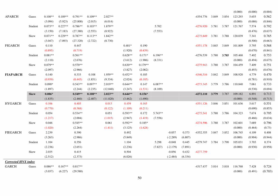
50

(0.000) (0.000) (0.004)

APARCH Gauss 0.108** 0.189** 0.791** 0.109** 2.027** -4354.776 3.849 3.854 123.293 5.655 0.562 (3.094) (5.923) (25.800) (2.015) (6.014) (0.000) (0.686) (0.846)

Student 0.073** 0.227** 0.786** 0.103** 1.879** 5.702 -4276.920 3.781 3.787 121.767 7.574 0.792

(3.150) (7.183) (27.380) (2.553) (8.922) (7.553) (0.476) (0.637)

Skew 0.071** 0.229** 0.787** 0.113** 1.842** -4275.849 3.781 3.788 120.039 7.341 0.765

(3.047) (7.093) (27.320) (2.722) (8.730) (0.500) (0.663)

FIGARCH Gauss 0.110 0.447 0.481* 0.190 -4351.178 3.845 3.849 101.809 5.795 0.568

(0.895) (0.719) (1.920) (0.439) (0.670) (0.841)

Student 0.081** 0.561** 0.628** 0.171* 6.196** -4276.539 3.780 3.785 105.468 7.402 0.753 (2.110) (2.676) (3.612) (1.906) (8.331) (0.000) (0.494) (0.675)

Skew 0.079** 0.570** 0.630** 0.179** -4275.943 3.780 3.787 104.459 7.409 0.751

(2.097) (2.966) (3.827) (2.082) (0.493) (0.676)

FIAPARCH Gauss 0.140 0.333 0.108 1.959** 0.452** 0.105 -4346.516 3.842 3.849 108.920 4.779 0.470

(0.939) (0.445) (1.851) (9.334) (2.024) (0.185) (0.781) (0.910)

Student 0.090* 0.543** 0.097** 2.019** 0.644** 0.147 6.087** -4273.345 3.779 3.786 110.840 7.061 0.733

(1.897) (2.244) (2.235) (12.040) (3.247) (1.531) (8.109) (0.530) (0.694)

Skew 0.086* 0.549** 0.108** 2.023** 0.644** 0.156* -4272.110 3.779 3.787 109.182 6.891 0.713

(1.835) (2.460) (2.407) (11.820) (3.462) (1.690) (0.000) (0.548) (0.713)

HYGARCH Gauss 0.106 0.405 0.013 0.459 0.165 -4351.126 3.846 3.851 101.636 5.617 0.551

(0.770) (0.368) (0.122) (1.109) (0.211) (0.690) (0.855)

Student 0.054 0.534** 0.051 0.593** 0.172 5.743** -4275.541 3.780 3.786 104.323 7.674 0.795

(1.217) (2.004) (1.015) (2.947) (1.419) (7.556) (0.466) (0.634)

Skew 0.046 0.545** 0.061 0.592** 0.185* -4274.596 3.780 3.787 102.601 7.689 0.796

(1.020) (2.264) (1.411) (3.125) (1.628) (0.000) (0.464) (0.73)

FIEGARCH Gauss 2.239 0.390 0.492 -0.057 0.373 -4352.355 3.847 3.852 106.745 4.109 0.408

(3.263) (2.986) (5.849) (-2.289) (6.807) (0.000) (0.904) (0.944)

Student 1.104 0.356 1.104 5.298 -0.048 0.445 -4279.747 3.784 3.790 105.031 3.703 0.374

(2.236) (2.651) (2.236) (7.827) (-2.179) (7.891) (0.000) (0.930) (0.958)

Skew 2.035 0.415 0.504 -0.056 0.432 -4277.759

(2.512) (2.373) (6.026) (-2.484) (6.334)

Corrected HNX index

GARCH Gauss 0.086** 0.167** 0.817** -4317.437 3.814 3.818 116.768 7.428 0.724 (3.037) (6.227) (29.580) (0.000) (0.491) (0.703)

51

Student 0.058** 0.202** 0.806** 6.240** -4259.105 3.764 3.768 116.714 9.241 0.943

(3.021) (7.427) (34.860) (7.235) (0.322) (0.492)

Skew 0.056** 0.204** 0.806** -4258.298 3.764 3.769 115.826 9.201 0.940

(2.888) (7.277) (34.480) (0.326) (0.495)

EGARCH Gauss 1.300 0.955 -0.021 0.291 -4346.148

(8.171) (81.080) (-1.056) (7.596)

Student 1.012 0.964 5.696 -0.038 0.356 -4270.370 3.774 3.780 116.718 4.301 0.396

(5.658) (95.840) (7.478) (-2.211) (9.108) (0.000) (0.890) (0.949)

Skew 2.286 0.965 -0.046 0.368 -4267.083 3.772 3.779 113.644 4.519 0.419

(3.441) (94.040) (-2.490) (8.799) (0.000) (0.874) (0.938)

GJR-GARCH Gauss 0.091** 0.142** 0.812** 0.057* -4313.723 3.812 3.816 121.095 5.743 0.560 (3.000) (6.862) (27.230) (1.666) (0.000) (0.676) (0.847)

Student 0.065** 0.172** 0.796** 0.077** 6.261** -4225.804 3.762 3.767 120.113 8.135 0.846

(3.103) (7.247) (32.060) (2.225) (7.153) (0.420) (0.584)

Skew 0.063** 0.171** 0.795** 0.086** -4254.426 3.761 3.768 118.582 7.961 0.828

(2.977) (7.153) (31.410) (2.363) (0.437) (0.602)

IGARCH Gauss 0.073** 0.183** 0.817 -4319.191 3.815 3.818 117.263 8.006 0.784 (3.122) (6.321) (-) (0.000) (0.433) (0.644) Student 0.062** 0.194** 0.806 6.461** -4259.279 3.763 3.767 116.672 8.932 0.904 (3.508) (8.453) (-) (7.799) (0.000) (0.348) (0.529)

Skew 0.062** 0.193** 0.807 -4258.614 3.763 3.768 115.956 8.821 0.891

(3.473) (8.370) (-) (0.358) (0.541)

RiskMetrics Gauss 0.060 0.940 -4374.795 3.864 3.867 107.733 36.647 3.192

(0.000) (0.000) (0.000) Student 0.060 0.940 6.417** -4307.921 3.806 3.809 106.122 36.601 3.191 (9.509) (0.000) (0.000) (0.000) Skew 0.060 0.940 -4305.969 3.805 3.810 104.235 36.568 3.192

(0.000) (0.000) (0.000)

APARCH Gauss 0.102** 0.165** 0.794** 0.075* 2.448** -4312.010 3.811 3.817 121.877 6.223 0.619 (2.895) (5.312) (26.570) (1.790) (6.188) (0.000) (0.622) (0.799) Student 0.066** 0.207** 0.791** 0.088** 2.151** 6.295** -4255.636 3.762 3.769 120.304 8.694 0.918 (3.015) (7.172) (29.160) (2.321) (8.398) (7.128) (0.000) (0.369) (0.515)

Skew 0.064** 0.212** 0.791** 0.098** 2.108** -4254.326 3.762 3.769 118.746 8.372 0.881

(2.912) (7.073) (29.070) (2.514) (8.291) (0.398) (0.550)

52

Notes: the numbers in parentheses are p-values of estimations. LL is the log-likelihood value. AIC, HQ correspond to the Akaike, Hannan-Quinn, respectively.

Q(10) and Q2(10)are, respectively, the Box Pierce statistics at lag10 of the standardized and squared standardized residuals. LM(10) is the ARCH LM test at lag 10.

** and * denote significance at the 1% and 5% levels, respectively.

FIGARCH Gauss 0.085 0.587 0.566** 0.241 -4312.299 3.811 3.815 103.060 6.301 0.612

(1.516) (1.856) (2.167) (1.829) (0.614) (0.805)

Student 0.066** 0.598** 0.635** 0.190** 6.733** -4255.120 3.761 3.766 104.750 7.473 0.751

(2.087) (3.299) (3.748) (2.472) (7.658) (0.000) (0.487) (0.677)

Skew 0.064** 0.608** 0.638** 0.197** -4254.177 3.761 3.767 103.691 7.462 0.747

(2.068) (3.737) (4.029) (2.644) (0.488) (0.681)

FIAPARCH Gauss 0.094 0.494 0.079 2.023** 0.518 0.195 -4309.487 3.810 3.816 107.905 4.792 0.466

(0.960) (0.702) (1.354) (12.170) (1.354) (0.507) (0.780) (0.913)

Student 0.059 0.553** 0.084** 2.165** 0.642** 0.153 6.394** -4251.642 3.760 3.767 109.201 7.462 0.782

(1.454) (2.108) (2.073) (12.840) (3.053) (1.467) (7.386) (0.488) (0.646)

Skew 0.053 0.558** 0.097** 2.182** 0.643** 0.162* -4249.839 3.759 3.767 107.297 7.200 0.752

(1.285) (2.339) (2.284) (12.640) (3.313) (1.642) (0.515) (0.676)

HYGARCH Gauss 0.092 0.602** -0.011 0.588** 0.237** -4312.208 3.811 3.817 103.467 6.450 0.627

(1.411) (2.027) (-0.286) (2.065) (2.141) (0.597) (0.792)

Student 0.041 0.570** 0.043 0.595** 0.196** 6.266** -4254.271 3.761 3.768 103.648 7.629 0.780

(1.013) (2.552) (0.962) (3.118) (2.002) (7.138) (0.471) (0.649)

Skew 0.034 0.581** 0.054 0.594** 0.209** -4252.936 3.761 3.768 101.876 7.606 0.776

(0.801) (2.938) (1.116) (3.349) (2.239) (0.473) (0.652)

FIEGARCH Gauss 2.091 0.411 0.495 -0.046 0.354 -4324.727 3.822 3.828 107.298 5.044 0.494

(3.053) (2.746) (5.248) (-2.062) (6.144) (0.000) (0.830) (0.895)

Student 1.126 0.343 0.559 5.642 -0.045 0.433 -4263.145 3.769 3.775 104.565 3.718 0.375

(2.166) (2.343) (6.808) (7.397) (-2.086) (7.600) (0.000 0.929) (0.958)

Skew 2.092 0.420 0.513 -0.053 0.416 -4260.935

(2.542) (2.063) (5.422) (-2.427) (5.697)

53

Table 5: Estimation results of different volatility models for Ho Chi Minh Stock exchanges (HOSE - VN index)

Model Distrib Parameters In-sample criteria Residuals tests

ω α β γ δ/k d ϕ v θ1 θ2 LL AIC HQ Q(10) Q2(10) LM(10)

GARCH Gauss 0.100** 0.161** 0.794** -3871.995 3.421 3.425 147.739 12.231 1.141

(2.927) (5.504) (19.680) (0.000) (0.141) (0.327)

Student 0.082** 0.193** 0.782** 9.861** -3850.972 3.403 3.408 142.691 14.479 1.491

(3.055) (5.950) (20.680) (4.742) (0.000) (0.070) (0.136)

Skew 0.078** 0.183** 0.790** -3847.837 3.401 3.407 144.348 14.265 1.438

(3.093) (6.085) (21.890) (0.000) (0.075) (0.157)

EGARCH Gauss 0.723 0.945 -0.032 0.255 -3883.713 3.432 3.437 146.608 17.722 1.634

(7.120) (58.060) (-2.229) (6.187) (0.000) (0.039) (0.091)

Student 0.593 0.951 8.546 -0.045 0.321 -3853.734 3.407 3.412 141.216 12.592 1.179

(4.719) (65.540) (5.317) (-2.891) (7.025) (0.000) (0.182) (0.300)

Skew 0.196 0.952 -0.040 0.313 -3852.844

(0.628) (68.060) (-2.550) (6.946)

GJR-GARCH Gauss 0.109** 0.128** 0.786** 0.070** -3867.301 3.418 3.422 152.337 10.447 0.995

(2.983) (5.659) (18.780) (2.378) (0.000) (0.235) (0.445)

Student 0.091** 0.152** 0.771** 0.089** 9.784** -3846.171 3.400 3.406 146.229 13.540 1.431

(3.218) (6.000) (19.940) (2.662) (4.719) (0.000) (0.095) (0.160)

Skew 0.087** 0.152** 0.779** 0.074** -3844.433 3.399 3.406 147.439 13.560 1.417

(3.202) (6.004) (20.650) (2.296) (0.000) (0.094) (0.166)

IGARCH Gauss 0.055** 0.179** 0.821 -3880.877 3.428 3.431 144.150 15.290 1.482

(2.591) (4.836) (0.000) (0.054) (0.140)

Student 0.063** 0.210** 0.790 8.489** -3852.705 3.404 3.408 139.779 16.480 1.786

(2.936) (5.612) (5.286) (0.000) (0.036) (0.058)

Skew 0.058** 0.202** 0.798 -3849.922 3.402 3.407 141.491 16.369 1.743

(2.961) (5.660) (0.000) (0.037) (0.066)

RiskMetrics Gauss 0.060 0.940 -3921.591 3.464 3.467 141.058 56.093 4.674

(0.000) (0.000) (0.000)

Student 0.060 0.940 9.675** -3892.780 3.439 3.443 140.035 55.639 4.647

(5.912) (0.000) (0.000) (0.000)

54

Skew 0.060 0.940 -3888.747 3.437 3.441 140.526 55.858 4.660

(0.000) (0.000) (0.000)

APARCH Gauss 0.113** 0.161** 0.780** 0.106** 2.105** -3867.177 3.419 3.424 152.766 10.204 0.979

(2.767) (5.534) (17.150) (2.874) (7.099) (0.000) (0.251) (0.460)

Student 0.087** 0.194** 0.780** 0.121** 1.824** 9.654** -3845.958 3.401 3.407 145.432 13.380 1.386

(3.043) (6.130) (19.070) (3.177) (7.308) (4.767) (0.000) (0.099) (0.181)

Skew 0.084** 0.187** 0.786** 0.103** 1.860** -3844.293 3.400 3.407 146.791 13.496 1.388

(3.033) (6.121) (19.670) (2.641) (7.391) (0.000) (0.096) (0.179)

FIGARCH Gauss 0.138** 0.199 0.344** 0.082 -3863.390 3.414 3.419 135.550 7.209 0.707

(2.264) (1.181) (5.666) (0.537) (0.514) (0.719)

Student 0.089** 0.375** 0.453** 0.166 10.398** -3843.221 3.397 3.403 133.238 9.461 0.977

(2.357) (2.641) (5.861) (1.491) (4.657) (0.305) (0.461)

Skew 0.083** 0.389** 0.445** 0.183* -3840.470 3.396 3.402 134.250 9.032 0.927

(2.319) (2.739) (5.710) (1.666) (0.000) (0.340) (0.507)

FIAPARCH Gauss 0.184** 0.235 0.131** 1.731** 0.348** 0.096 -3858.035 3.411 3.418 140.375 7.287 0.698

(2.709) (1.599) (2.836) (10.430) (6.238) (0.733) (0.506) (0.728)

Student 0.128** 0.382** 0.139** 1.719** 0.455** 0.154* 10.445** -3837.842 3.394 3.402 137.522 9.305 0.936

(2.918) (3.148) (3.121) (9.312) (6.465) (1.645) (4.654) (0.000) (0.317) (0.499)

Skew 0.122** 0.396** 0.119** 1.745** 0.455** 0.167 -3836.600 3.394 3.402 138.179 9.163 0.924

(2.866) (3.210) (2.586) (9.575) (6.300) (1.776) (0.329) (0.510)

HYGARCH Gauss 0.168** 0.276 -0.055 0.395** 0.124 -3863.082 3.415 3.420 137.080 7.210 0.707

(2.011) (1.436) (-0.710) (3.652) (0.822) (0.514) (0.719)

Student 0.083 0.365** 0.009 0.444** 0.163 10.315** -3843.029 3.398 3.405 132.902 9.450 0.977

(1.404) (2.252) (0.151) (4.120) (1.412) (4.605) (0.306) (0.461)

Skew 0.084 0.391** -0.002 0.447** 0.184* -3840.469 3.397 3.404 134.319 9.039 0.927

(1.505) (2.448) (-0.033) (4.009) (1.665) (0.339) (0.507)

FIEGARCH Gauss 0.959 0.451 0.429 -0.060 0.322 -3863.448 3.415 3.421 133.468 8.165 0.779

(3.515) (3.800) (6.661) (-3.414) (6.979) (0.000) (0.518) (0.650)

Student 0.672 0.494 0.463 9.280 -0.064 0.349 -3840.146 3.396 3.402 132.574 7.959 0.765

(2.147) (4.139) (7.607) (4.885) (-3.736) (7.206) (0.000) (0.538) (0.663)

Skew 0.941 0.496 0.463 -0.066 0.345 -3839.929

(1.179) (4.346) (7.815) (-3.821) (7.045)

55

Notes: the numbers in parentheses are p-values of estimations. LL is the log-likelihood value. AIC, HQ correspond to the Akaike, Hannan-Quinn, respectively.

Q(10) and Q2(10) are, respectively, the Box Pierce statistics at lag10 of the standardized and squared standardized residuals. LM(10) is the ARCH LM test at lag 10.

** and * denote significance at the 1% and 5% levels, respectively.

56

Table 6: VaR forecast evaluation for HNX index

Model Distrib. Parameters

Quantile Failure (LRT) DQT ESF VaR 5% VaR 1%

HNX-index GARCH Gauss 0.050 0.033 6.562 7.605 -3.418

0.010 0.369

EGARCH (1,0) Student 0.050 0.034 5.745 6.642 -3.400

0.017 0.467

GJR-GARCH Gauss 0.050 0.032 7.441 8.070 -3.486

0.006 0.326

IGARCH Gauss 0.050 0.035 4.989 6.352 -3.323

0.026 0.499

Student 0.050 0.038 3.071 5.643 -3.207 -2.461 -3.485 0.080 0.582

Riskmetrics Gauss 0.050 0.049 0.006 4.829 -3.137 -2.035 -2.883 0.936 0.681

Student 0.050 0.049 0.006 4.828 -3.137 -2.059 -2.917 0.936 0.681

Skew 0.050 0.057 0.850 6.158 -2.979 -2.045 -2.896 0.357 0.521

APARCH Gauss 0.050 0.032 7.441 8.079 -3.486

0.006 0.326

FIGARCH Student 0.050 0.039 2.543 5.332 -3.189 -2.519 -3.568 0.111 0.620

FIAPARCH Skew 0.050 0.042 1.274 5.315 -3.108 -2.473 -3.503 0.259 0.622

FIEGARCH (1,d,0) Gauss 0.050 0.036 4.293 6.970 -3.376

0.038 0.432

Student 0.050 0.035 4.989 11.539 -3.390

0.026 0.117

HNX-index corrected GARCH Gauss 0.050 0.035 4.989 6.306 -3.333

0.026 0.505

EGARCH (1,0) Student 0.050 0.034 5.745 6.628 -3.400

0.017 0.469

Skew 0.050 0.044 0.679 3.141 -3.104 -2.364 -3.348 0.410 0.872

GJR-GARCH Gauss 0.050 0.034 5.745 6.507 -3.446

0.017 0.482

IGARCH Gauss 0.050 0.037 3.654 5.361 -3.248 -2.406 -3.408 0.056 0.616

Student 0.050 0.038 3.071 5.517 -3.207 -2.400 -3.399 0.080 0.597

Riskmetrics Gauss 0.050 0.049 0.006 4.830 -3.137 -2.036 -2.884 0.936 0.681

Student 0.050 0.049 0.006 4.827 -3.137 -2.056 -2.913 0.936 0.681

Skew 0.050 0.057 0.850 6.156 -2.979 -2.041 -2.891 0.357 0.522

APARCH Gauss 0.050 0.034 5.745 6.862 -3.351

0.017 0.443

Student 0.050 0.036 4.293 5.877 -3.244

0.038 0.554

FIGARCH Student 0.050 0.039 2.543 5.199 -3.189 -2.447 -3.466

57

Notes: In the dynamic quantile regression, p = 5. The best model is one with the least rejections. The p-values for

the Kupiec’s (1995) and Manganelli (2004) tests are displayed in parentheses. ESF refers to the expected shortfall.

VaR(1%) and VaR(5%) correspond to VaR at 1% and 5% level, respectively.

0.111 0.636

FIEGARCH (1,d,0) Gauss 0.050 0.038 3.071 5.466 -3.363 -2.143 -3.036

0.080 0.603

Student 0.050 0.034 5.745 6.626 -3.400

0.017 0.469

58

Table 7: VaR forecast evaluation for VN-index

Model Distrib. Parameters

Quantile Failure (LRT) DQT ESF VaR 5% VaR 1%

VN-index

GARCH Gauss 0.050 0.039 2.543 11.691 -2.862 -2.021 -2.862 0.111 0.111

Student 0.050 0.042 1.274 16.614 -2.776 -2.021 -2.862 0.259 0.020

Skew 0.050 0.034 5.745 .NaN -2.714

0.017 0.000

EGARCH Gauss 0.050 0.035 4.989 9.057 -2.926

0.026 0.249

Student 0.050 0.041 1.646 8.466 -2.772 -1.950 -2.761 0.200 0.293

GJR-GARCH Gauss 0.050 0.039 2.543 11.329 -2.862 -2.008 -2.844 0.111 0.125

Student 0.050 0.039 2.543 10.067 -2.770 -2.008 -2.844 0.111 0.185

Skew 0.050 0.031 8.385 .NaN -2.667

0.004 0.000

IGARCH Gauss 0.050 0.041 1.646 10.478 -2.771 -2.018 -2.858 0.200 0.163

Student 0.050 0.044 0.679 12.555 -2.677 -2.018 -2.858 0.410 0.084

Skew 0.050 0.040 2.068 10.595 -2.720 -2.015 -2.855 0.150 0.157

Riskmetrics Gauss 0.050 0.049 0.006 11.171 -2.672 -1.781 -2.523 0.936 0.131

Student 0.050 0.053 0.247 13.128 -2.556 -1.781 -2.522 0.619 0.069

Skew 0.050 0.049 0.006 11.113 -2.672 -1.782 -2.524 0.936 0.134

APARCH Gauss 0.050 0.039 2.543 11.350 -2.862 -2.030 -2.875 0.111 0.124

Student 0.050 0.040 2.068 10.279 -2.822 -2.030 -2.875 0.150 0.173

Skew 0.050 0.030 9.396 .NaN -2.645

0.002 0.000

FIGARCH Skew 0.050 0.037 3.654 .NaN -2.626

0.056 0.000

FIAPARCH Student 0.050 0.047 0.140 10.966 -2.657 -1.845 -2.613 0.708 0.140

FIEGARCH (1,d,0) Gauss 0.050 0.047 0.140 7.063 -2.716 -1.768 -2.504

0.708 0.422

59

Notes: In the dynamic quantile regression, p = 5. The best model is one with the least rejections. The p-values for the

Kupiec’s (1995) and Manganelli (2004) tests are displayed in parentheses. ESF refers to the expected shortfall.

Student 0.050 0.043 0.952 6.062 -2.757 -1.924 -2.725

0.329 0.533