Embed Size (px)
Citation preview

ISNB 978-9984-888-20-0
GINTERS BUŠS
FORECASTING AND SIGNAL EXTRACTION WITH
REGULARISED MULTIVARIATE DIRECT FILTER APPROACH
WORKING PAPER
6 / 2012
© Latvijas Banka, 2012
This source is to be indicated when reproduced.

1
FORECASTING AND SIGNAL EXTRACTION WITH REGULARISED MULTIVARIATE DIRECT FILTER APPROACH
CONTENTS
Abstract 2 Introduction 3 1. Regularised Multivariate Direct Filter Approach 4 1.1 Univariate direct filter approach 5 1.2 Multivariate direct filter approach 6 1.3 Rewriting filtration problem in a least squares form 7 1.4 Regularisation 8 1.5 Level and time shift constraints 10 1.6 Effective degrees of freedom 11 2. Tracking Economic Activity in the Euro Area 11 2.1 Tracking trendcycle in yearly growth of GDP 11 2.1.1 Target 12 2.1.2 Explanatory variables 12 2.1.3 Regularisation features 12 2.1.4 Indicator design 22 2.2 Tracking trendcycle in quarterly growth of GDP 26 2.2.1 Target and data 26 2.2.2 Indicator design 26 3. Robustness Check on Less Homogeneous Dataset for Latvia 30 Conclusions 34 Appendix 34 Bibliography 38
ABBREVIATIONS
CSB – Central Statistical Bureau DE – Germany d.f. – degrees of freedom DFT – discrete Fourier transform DG Ecfin – Directorate General for Economic and Financial Affairs (e.)d.f. – (effective) degrees of freedom EA – euro area EE – Estonia ES – Spain EU – European Union Eurocoin – Euro Area Business Cycle Coincidence Indicator FR – France GDP – gross domestic product IT – Italy Latcoin – Latvian Business Cycle Coincidence Indicator LT – Lithuania LV – Latvia MSFE – mean squared filter error NSA – seasonally unadjusted q-o-q – quarter-on-quarter RMDFA – regularised multivariate direct filter approach SA – seasonally adjusted US – United States w.r.t. – with respect to y-o-y – year-on-year
2
FORECASTING AND SIGNAL EXTRACTION WITH REGULARISED MULTIVARIATE DIRECT FILTER APPROACH
ABSTRACT
The paper studies regularised direct filter approach as a tool for high-dimensional filtering and real-time signal extraction. It is shown that the regularised filter is able to process high-dimensional data sets by controlling for effective degrees of freedom and that it is computationally fast. The paper illustrates the features of the filter by tracking the medium-to-long-run component in GDP growth for the euro area, including replication of Eurocoin-type behavior as well as producing more timely indicators. A further robustness check is performed on a less homogeneous dataset for Latvia. The resulting real-time indicators are found to track economic activity in a timely and robust manner. The regularised direct filter approach can thus be considered a promising tool for both concurrent estimation and forecasting using high-dimensional datasets and a decent alternative to the dynamic factor methodology.
Keywords: high-dimensional filtering, real-time estimation, coincident indicator, leading indicator, parameter shrinkage, business cycles, dynamic factor model
JEL codes: C13, C32, E32, E37
The author thanks Marc Wildi for valuable discussions. All remaining errors are the author's own. Disclaimer: This report is released to inform interested parties of research and to encourage discussion. The views expressed in this paper are those of the author and do not necessarily reflect the views of the Bank of Latvia.
3
FORECASTING AND SIGNAL EXTRACTION WITH REGULARISED MULTIVARIATE DIRECT FILTER APPROACH
INTRODUCTION
Nowadays, gathering rich datasets is relatively easy. A more difficult exercise is effectively using them for a particular problem at hand. This paper adds to the literature on forecasting, regularisation, shrinkage, and high-dimensional estimation (see, ridge regression in, e.g. Tikhonov and Arsenin (1977) and Hoerl and Kennard (1970), lasso in Tibshirani (1996), least angle regression in Efron et al. (2004), Bayesian shrinkage in, e.g. Doan, Litterman and Sims (1984), factor models in Stock and Watson (2002) and Forni et al. (2000), (2005)) by exploring the properties of a regularised multivariate direct filter approach (RMDFA in short (Wildi (2012)) in signal extraction and forecasting using many variables.
Wildi (2012) derives the regularised multivariate filter as a successor to an unregularised direct filter approach (Wildi (2011)) but does not study its properties either using generated or real-world data. Thus, this paper is the first paper known to the author that studies and implements the RMDFA to data. Furthermore, this paper studies how the RMDFA could be implemented to high-dimensional real-world datasets. This paper finds that filter regularisation helps in real-time signal extraction, since it controls for effective degrees of freedom, thus allowing to control for overfitting that can have degrading effects on out-of-sample performance. Another advantage of a regularised filter is that it allows for high-dimensional data to enter the filter and, therefore, further robustify the outcome. As it is shown in the paper, a particular regularisation feature used in the paper might remind about the "lag decay" term in Minnessota prior (e.g. Doan, Litterman and Sims (1984)) in Bayesian econometrics. Forcing more distant filter coefficients to zero both saves degrees of freedom and effectively shortens the filter, thus making it more responsive to the changing environment. Another regularisation feature studied in this paper is cross-sectional shrinkage that makes filter coefficients to behave similarly for similar series. The cross-sectional shrinkage has been found useful, particularly so if the dataset is rather homogeneous.
As an application, the filter is applied to up to 72 variables in order to track the medium-to-long-run component of the euro area GDP growth. Both yearly and quarterly growth rates of GDP are considered. The results show that the filter output is robust and able to mimic as well as to produce more timely indicators than an established Eurocoin indicator (Altissimo et al. (2010)) that is based on the dynamic factor methodology (Forni et al. (2000), (2005)). Comparison of the RMDFA to the dynamic factor methodology of Forni et al. (2005) is especially important, since both methods have much in common and also feature some clear-cut differences. First, while the dynamic factor methodology shrinks the dimension of dataset to a few unobserved factors and, thus, has a few parameters to estimate, the RMDFA does not shrink the dimension of dataset but rather imposes restrictions on coefficient behavior. Therefore, the RMDFA can be involved in computing hundreds or even thousands of coefficients. Nonetheless, controlling for effective degrees of freedom helps avoid the overparameterisation problem and, thus, achieve good out-of-sample behavior. The paper illustrates this point by computing more than 800 filter coefficients for less than 150 observations long sample. Second, the dynamic factor methodology of Forni et al. (2005), as most other factor methods, including Stock and Watson (2002), extracts factors from the explanatory dataset independently of what is the target variable. If irrelevant variables dominate the dataset, the extracted generalised principal components would have little in common
4
FORECASTING AND SIGNAL EXTRACTION WITH REGULARISED MULTIVARIATE DIRECT FILTER APPROACH
with the target. Thus, careful pre-selection of explanatory variables is a prerequisite for a successful application of the factor methodology. By contrast, the RMDFA is more robust to such an error, since the filter would put smaller weights on irrelevant variables, and higher weights on more relevant ones. Therefore, the RMDFA requires potentially less work in the variable pre-selection step.
As a robustness check, the filter is applied to a less homogeneous dataset for Latvia and is proved to stand the test.
The paper is structured as follows. Section 1 introduces new regularisation features in the direct filter approach. Subsections 2.1 and 2.2 illustrate the new features of the filter by creating indicators for yearly and quarterly growth rates of the euro area GDP respectively. Section 3 performs a robustness check on a less homogeneous dataset for Latvia. Appendix lists the data and their transformations.
1. REGULARISED MULTIVARIATE DIRECT FILTER APPROACH
Regularised multivariate direct filter approach is a regularised version of the multivariate direct filter approach (Wildi (2011)), which has been found to be useful in creating real-time indicators (Bušs (2012)).
However, the unregularised multivariate direct filter contains many parameters whose number increases with filter's dimension. Thus, the filter in Wildi (2011) cannot be too long or cannot contain tens of macroeconomic variables due to the limited sample size typically observed in macroeconomics, otherwise the filter would be overparameterised and the filter output would have poor out-of-sample quality. One way of increasing the cross-sectional dimension of the filter would be to decrease the length of the filter accordingly, and that indeed has been coded in the algorithm used in Bušs (2012). However, the length of the filter cannot be decreased infinitely, since it is bounded to zero, while too short a filter would result in deteriorating quality of its output. Therefore, similar to standard econometric practices in parameter shrinkage (ridge regression in, e.g. Tikhonov and Arsenin (1977) and Hoerl and Kennard (1970), lasso in Tibshirani (1996), least angle regression in Efron et al. (2004), Bayesian shrinkage in, e.g. Doan, Litterman and Sims (1984)), it would be reasonable to attempt to shrink the filter parameters as well in order to allow for controlling for effective degrees of freedom and using high-dimensional datasets. Such an attempt is made in Wildi (2012) that introduces three shrinkage parameters in a multivariate direct filter approach (Wildi (2011)) that control for cross-sectional shrinkage and shrinkage along time dimension and impose smoothness of filter coefficients. The three shrinkage dimensions can be imposed in any of their combinations or all of them can be set to zero so that the new filter replicates the one discussed in Wildi (2011).
In order to introduce the new regularisation features, this paper builds on the classical filtration problem. Since details on technicalities can be found in Wildi (2011), (2012), this section just summarises the main elements of a customised filter necessary to introduce the new regularisation features later in the section.
We denote as the output of a symmetric, possibly bi-infinite filter ∑ applied to input series :
5
FORECASTING AND SIGNAL EXTRACTION WITH REGULARISED MULTIVARIATE DIRECT FILTER APPROACH
∑
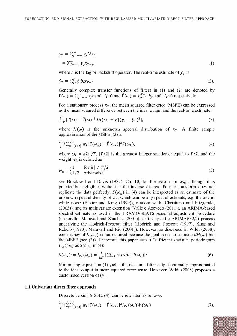
∑ , (1)
where is the lag or backshift operator. The real-time estimate of is
∑ (2).
Generally complex transfer functions of filters in (1) and (2) are denoted by Γ ∑ exp and Γ ∑ exp respectively.
For a stationary process , the mean squared filter error (MSFE) can be expressed as the mean squared difference between the ideal output and the real-time estimate:
|Γ Γ | , (3)
where is the unknown spectral distribution of . A finite sample approximation of the MSFE, (3) is
∑ // |Γ Γ | , (4)
where 2 / , /2 is the greatest integer smaller or equal to /2, and the weight is defined as
1 for| | /21/2 otherwise, (5)
see Brockwell and Davis (1987), Ch. 10, for the reason for ; although it is practically negligible, without it the inverse discrete Fourier transform does not replicate the data perfectly. in (4) can be interpreted as an estimate of the unknown spectral density of , which can be any spectral estimate, e.g. the one of white noise (Baxter and King (1999)), random walk (Christiano and Fitzgerald, (2003)), and its multivariate extension (Valle e Azevedo (2011)), an ARIMA-based spectral estimate as used in the TRAMO/SEATS seasonal adjustment procedure (Caporello, Maravall and Sánchez (2001)), or the specific ARIMA(0,2,2) process underlying the Hodrick-Prescott filter (Hodrick and Prescott (1997), King and Rebelo (1993), Maravall and Rio (2001)). However, as discussed in Wildi (2008), consistency of is not required because the goal is not to estimate but the MSFE (see (3)). Therefore, this paper uses a "sufficient statistic" periodogram
as in (4):
: |∑ exp | (6).
Minimising expression (4) yields the real-time filter output optimally approximated to the ideal output in mean squared error sense. However, Wildi (2008) proposes a customised version of (4).
1.1 Univariate direct filter approach
Discrete version MSFE, (4), can be rewritten as follows:
∑ // |Γ Γ | (7),
6
FORECASTING AND SIGNAL EXTRACTION WITH REGULARISED MULTIVARIATE DIRECT FILTER APPROACH
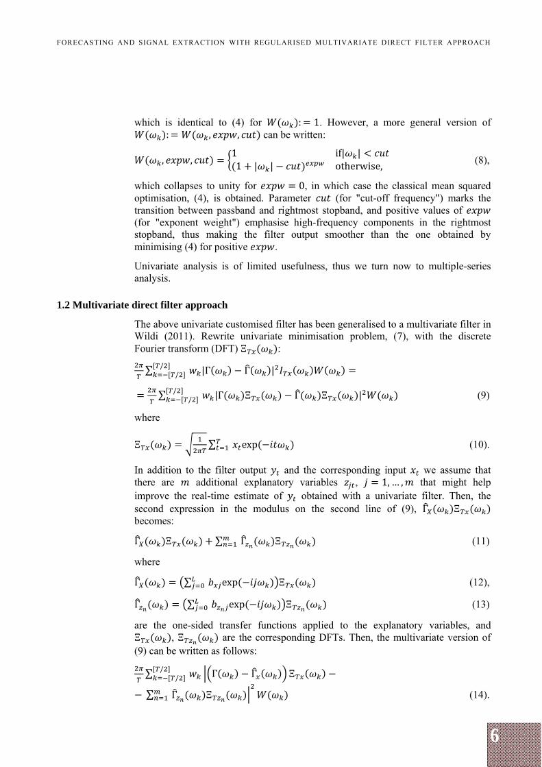
which is identical to (4) for : 1. However, a more general version of : , , can be written:
, ,1 if| |1 | | otherwise, (8),
which collapses to unity for 0, in which case the classical mean squared optimisation, (4), is obtained. Parameter (for "cut-off frequency") marks the transition between passband and rightmost stopband, and positive values of (for "exponent weight") emphasise high-frequency components in the rightmost stopband, thus making the filter output smoother than the one obtained by minimising (4) for positive .
Univariate analysis is of limited usefulness, thus we turn now to multiple-series analysis.
1.2 Multivariate direct filter approach
The above univariate customised filter has been generalised to a multivariate filter in Wildi (2011). Rewrite univariate minimisation problem, (7), with the discrete Fourier transform (DFT) Ξ :
∑ // |Γ Γ |
∑ // |Γ Ξ Γ Ξ | (9)
where
Ξ ∑ exp (10).
In addition to the filter output and the corresponding input we assume that there are additional explanatory variables , 1,… , that might help improve the real-time estimate of obtained with a univariate filter. Then, the second expression in the modulus on the second line of (9), Γ Ξ becomes:
Γ Ξ ∑ Γ Ξ (11)
where
Γ ∑ exp Ξ (12),
Γ ∑ exp Ξ (13)
are the one-sided transfer functions applied to the explanatory variables, and Ξ , Ξ are the corresponding DFTs. Then, the multivariate version of (9) can be written as follows:
∑ // Γ Γ Ξ
∑ Γ Ξ (14).
7
FORECASTING AND SIGNAL EXTRACTION WITH REGULARISED MULTIVARIATE DIRECT FILTER APPROACH
1.3 Rewriting filtration problem in a least squares form
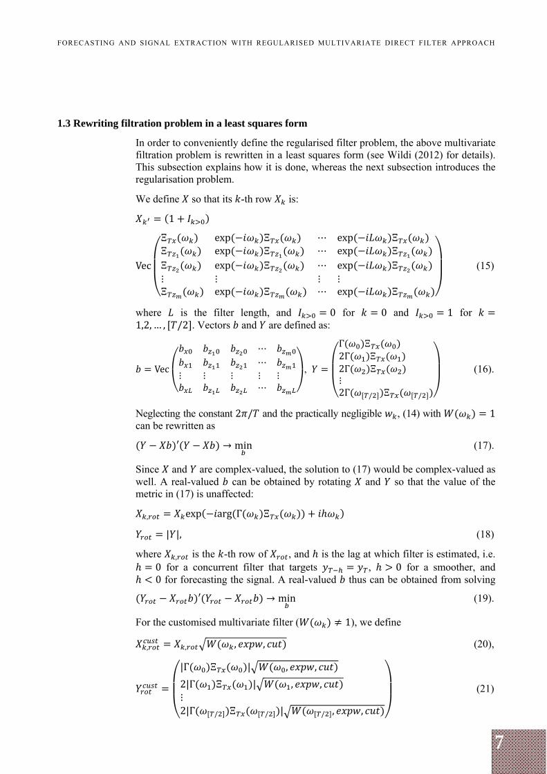
In order to conveniently define the regularised filter problem, the above multivariate filtration problem is rewritten in a least squares form (see Wildi (2012) for details). This subsection explains how it is done, whereas the next subsection introduces the regularisation problem.
We define so that its -th row is:
1
Vec
Ξ exp Ξ ⋯ exp ΞΞ exp Ξ ⋯ exp ΞΞ exp Ξ ⋯ exp Ξ⋮ ⋮ ⋮ ⋮Ξ exp Ξ ⋯ exp Ξ
(15)
where is the filter length, and 0 for 0 and 1 for 1,2, … , /2 . Vectors and are defined as:
Vec
⋯⋯
⋮ ⋮ ⋮ ⋮ ⋮⋯
,
Γ Ξ2Γ Ξ2Γ Ξ⋮2Γ / Ξ /
(16).
Neglecting the constant 2 / and the practically negligible , (14) with 1 can be rewritten as
′ → min (17).
Since and are complex-valued, the solution to (17) would be complex-valued as well. A real-valued can be obtained by rotating and so that the value of the metric in (17) is unaffected:
, exp arg Γ Ξ
| |, (18)
where , is the -th row of , and is the lag at which filter is estimated, i.e. 0 for a concurrent filter that targets , 0 for a smoother, and 0 for forecasting the signal. A real-valued thus can be obtained from solving
′ → min (19).
For the customised multivariate filter ( 1), we define
, , , , (20),
|Γ Ξ | , ,
2|Γ Ξ | , ,⋮2|Γ / Ξ / | / , ,
(21)
8
FORECASTING AND SIGNAL EXTRACTION WITH REGULARISED MULTIVARIATE DIRECT FILTER APPROACH
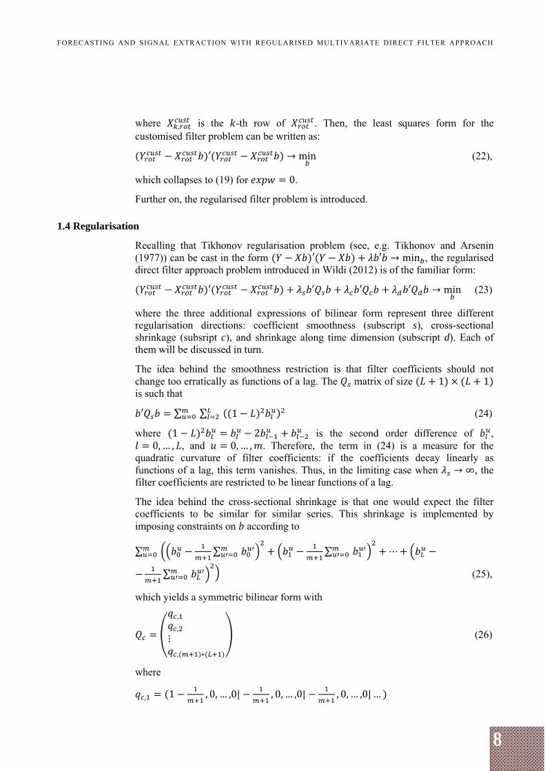
where , is the -th row of . Then, the least squares form for the customised filter problem can be written as:
′ → min (22),
which collapses to (19) for 0.
Further on, the regularised filter problem is introduced.
1.4 Regularisation
Recalling that Tikhonov regularisation problem (see, e.g. Tikhonov and Arsenin (1977)) can be cast in the form ′ ′ → min , the regularised direct filter approach problem introduced in Wildi (2012) is of the familiar form:
′ ′ ′ ′ → min (23)
where the three additional expressions of bilinear form represent three different regularisation directions: coefficient smoothness (subscript s), cross-sectional shrinkage (subsript c), and shrinkage along time dimension (subscript d). Each of them will be discussed in turn.
The idea behind the smoothness restriction is that filter coefficients should not change too erratically as functions of a lag. The matrix of size 1 1 is such that
′ ∑ ∑ 1 (24)
where 1 2 is the second order difference of , 0, … , , and 0,… , . Therefore, the term in (24) is a measure for the
quadratic curvature of filter coefficients: if the coefficients decay linearly as functions of a lag, this term vanishes. Thus, in the limiting case when → ∞, the filter coefficients are restricted to be linear functions of a lag.
The idea behind the cross-sectional shrinkage is that one would expect the filter coefficients to be similar for similar series. This shrinkage is implemented by imposing constraints on according to
∑ ∑ ∑ ⋯
∑ (25),
which yields a symmetric bilinear form with
,
,
⋮, ∗
(26)
where
, 1 , 0, … ,0| , 0, … ,0| , 0, … ,0|…
9
FORECASTING AND SIGNAL EXTRACTION WITH REGULARISED MULTIVARIATE DIRECT FILTER APPROACH
, 0,1 , 0, … ,0|0, , 0, … ,0|0 , 0, … ,0|…
, 0,0,1 , 0, … ,0|0,0, , 0, … ,0|0,0, , 0, … ,0|…
… , ∗ 0,0, … , |0,0, … , |0,0, … , | …
|0,0, … ,1 (27),
so that each block separated by | is of length 1. Thus, there are 1's on the
diagonal of and periodically arranged 's, which account for the central
means in (25).
A higher gives preference for more similar filters across series, and the limiting case → ∞ ensures that the filter coefficients are identical across series.
Finally, the idea behind the shrinkage across time dimension is that a practitioner might give preference for the filter coefficients that decay to zero progressively as functions of a lag. For a Bayesian econometrician, this would remind of the lag decay in the Minnesota prior (see, e.g. Doan, Litterman and Sims (1984)). This shrinkage is implemented by setting so that
′ ∑ ∑ (28)
where is the -th element of
∨ , | ∨ |, | ∨ |, … , | ∨ | (29)
where is set to : 1 , ∨ denotes themax ⋅ function, and signifies the lag at which filter is estimated, i.e. 0 means a concurrent filter that targets
, 0 means that the filter is the smoother, and 0 means that the filter is targeted to forecast the signal periods ahead. When estimating for
0, a practitioner would want to assign the largest filter weight to observations coinciding with . Thus, (29) ensures that minimum regularisation is imposed on lag (since ∨ ), and a decay is emphasised symmetrically on both sides away from the target lag . A higher ensures a faster coefficient decay to zero as a function of the lag.
Since the regularisation is cast in bilinear forms, the problem in (23) has an analytic solution. Setting 0 gives the unregularised filter problem in (22). Or, setting 0 but letting some of the regularisation lambdas positive gives the regularised classical multivariate filter problem. It has been found in this paper that the lag decay shrinkage is the most useful of the three regularisation types for the application at hand, followed by the cross-sectional shrinkage.
The next section describes an application of the filter obtained by solving (23) subject to two potential constraints: first and/or second order constraints, which are explained in the following subsection.
10
FORECASTING AND SIGNAL EXTRACTION WITH REGULARISED MULTIVARIATE DIRECT FILTER APPROACH
1.5 Level and time shift constraints
The first order constraint imposes specific values on amplitude functions in frequency zero. For a bandpass, one would typically set amplitudes at frequency zero to be zero, ensuring that a bandpass puts zero weight on trend frequency, while for a univariate lowpass one would typically set amplitude at frequency zero to unity, to ensure that a lowpass tracks the level/scale of the target; such a restriction is related to assuming that the target has a unit root at frequency zero, i.e. it is a first order integrated process.
For a multivariate filter, the optimal constrained level of the amplitude at frequency zero is less clearly cut. This level can be set to an inverse of the number of explanatory variables for all of the variables, if all explanatory variables follow about the same trend. However, the latter might not always be the case, and, thus, a better outcome could be obtained by differentiating the amplitude constraint at frequency zero for various explanatory variables. An example of such a differentiation of the constraint is provided in the empirical section.
In practice, one can choose between using or not using the level constraint at ones own discretion. This constraint is implemented by the following restriction:
⋯ (30)
where is the value at which the transfer function for variable is set at frequency zero, and is the targeted lag ( 0 for a concurrent filter, 0 for a smoother, and 0 for forecasting the signal).
The second order constraint restricts the time shift of the filter at zero frequency to vanish, and is related to assuming that the target variable has two unit-roots in frequency zero, in which case the first and the second order constraints would be both implemented. In practice, however, the usage of the constraints are up to the practitioner's agenda, and one could use the time shift constraint without imposing the level constraint, the combination of the constraints that can not be straightforwardly imposed in the time domain. The second order constraint is imposed by forcing the derivative of the transfer function at frequency zero to vanish, which results in the following coefficient constraint:
1 2 ⋯ 2 ⋯
0 (31)
where is the targeted lag ( 0 for a concurrent filter, 0 for a smoother, and 0 for forecasting the signal).
Both constraints can be implemented by selecting any two of the coefficients but is implemented by constraining and , so as to avoid a conflicting situation between these constraints and the regularisation, e.g. a lag decay agenda for large enough.
The constrained regularised filter problem is solved by rewriting filter coefficient vector as follows:
, (32)
11
FORECASTING AND SIGNAL EXTRACTION WITH REGULARISED MULTIVARIATE DIRECT FILTER APPROACH
where is the vector of freely determined filter coefficients, plugging (32) in (23), solving for , and then plugging the estimate of in (32) to get the estimate of (see Wildi (2012) for details).
1.6 Effective degrees of freedom
In an unconstrained ordinary least squares framework, the (regression) degrees of freedom are the number of estimated parameters. Given a well-posed ordinary least squares problem ′ → min, the fitted values of can be written in
terms of a hat or smoother matrix S, which is just a projection matrix P:
′ ′ (33).
The degrees of freedom are the trace of projection matrix:
. . (34),
which equals to rank .
For a regularised problem as in expression (23), ′′ ′ ′ → min the smoother matrix is no longer
an orthogonal projection but the same notion applies. Denoting the fitted value of by and the corresponding smoother matrix by , we obtain:
′ ′ (35),
so that , and the effective degrees of freedom (or, effective number of parameters) are the trace of :
. . . (36)
(see, e.g. Moody (1992), Hodges and Sargent (2001)).
Effective degrees of freedom are useful in controlling for an overfitting and, consequently, in controlling for an out-of-sample performance.
2. TRACKING ECONOMIC ACTIVITY IN THE EURO AREA
2.1 Tracking trendcycle in yearly growth of GDP
This section discusses the new regularisation features of the multivariate filter by creating two real-time indicator designs for the euro area GDP. The two indicator designs differ by the input data transformation and according modifications in their filter designs. The first design discussed in this subsection considers yearly growth rates of real GDP, while the second one discussed in the next subsection considers quarterly growth rates of real GDP. Potential users of those indicators then can form a subjective preference between the two. More discussion follows in the respective subsections focusing on each design separately, starting with the yearly growth design.
12
FORECASTING AND SIGNAL EXTRACTION WITH REGULARISED MULTIVARIATE DIRECT FILTER APPROACH
2.1.1 Target
The filter is set to target an ideal lowpass of yearly growth of real GDP with cut-off wave length 12 months. The quarterly GDP data are taken from the first quarter of 1995 onwards as published by the Eurostat. The data are linearly interpolated to monthly frequency, logged, yearly differenced and demeaned before their spectral content enters the filter.
2.1.2 Explanatory variables
Monthly business and consumer confidence indicators published by DG Ecfin and other monthly variables are used as explanatory variables. In total, 72 monthly variables are used. The choice of the indicators is based on economic relevance and data availability. Appendix contains a complete list of input data and their transformations. DG Ecfin data are usually published at the end of the reference month, except December, for which data are published in early January. DG Ecfin business and consumer survey data are almost unrevised: this applies both to seasonally unadjusted and seasonally adjusted data, as the latter is the product of the seasonal adjustment program Dainties, which does not revise historic data as new ones come in1. The above-mentioned considerations make DG Ecfin data convenient for real-time filtration. Some other explanatory data happen to be revised but the effect of their revision on the filter output is considered to be of minor extent and, therefore, the final revision data are used.
All explanatory variables are taken from January 1995 onwards, standardised to zero mean and unit variance. Integrated data are made non-integrated by suitable transformations. Appendix lists the data and their transformations.
2.1.3 Regularisation features
We now examine the regularisation features of the filter. For visual tractability and due to numerical issues (an unregularised filter crashes for a high-dimensional input data when the number of estimated filter parameters reaches that of sample observations), only nine survey variables are used to analyse the filter effect. More data are added further on in the section. The nine variables are business and consumer confidence data: production trend observed in recent months (industry), assessment of order-book levels (industry), assessment of stocks of finished products (industry), production expectations for the months ahead (industry), employment expectations for the months ahead (industry), confidence indicator in construction, confidence indicator in retail, consumer confidence indicator, and confidence indicator in services.
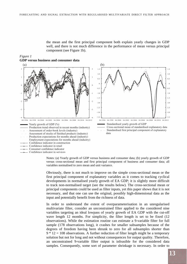
In order to motivate the chosen transformation of data, it is illustrative to plot the transformed target variable and explanatory variables. Figure 1a shows standardised yearly growth of EA GDP versus standardised business and consumer data. Explanatory data are well aligned with the yearly growth of GDP. Extracting the cross-sectional mean and the first principal component of the standardised explanatory data, and plotting against standardised yearly growth of GDP shows that 1 For details, see The joint harmonized EU programme of business and consumer surveys, User Guide,
2007, European Commission Directorate-General for Economic and Financial Affairs, available at http://ec.europa.eu/economy_finance/db_indicators/surveys/documents/userguide_en.pdf
13
FORECASTING AND SIGNAL EXTRACTION WITH REGULARISED MULTIVARIATE DIRECT FILTER APPROACH
the mean and the first principal component both explain yearly changes in GDP well, and there is not much difference in the performance of mean versus principal component (see Figure 1b).
Figure 1 GDP versus business and consumer data
Notes: (a) Yearly growth of GDP versus business and consumer data; (b) yearly growth of GDP versus cross-sectional mean and first principal component of business and consumer data; all variables normalised to zero mean and unit variance. Obviously, there is not much to improve on the simple cross-sectional mean or the first principal component of explanatory variables as it comes to tracking cyclical developments in normalised yearly growth of EA GDP; it is slightly more difficult to track non-normalised target (see the results below). The cross-sectional mean or principal components could be used as filter inputs, yet this paper shows that it is not necessary, and that one can use the original, possibly high-dimensional data as the input and potentially benefit from the richness of data.
In order to understand the extent of overparameterisation in an unregularised multivariate filter, consider an unconstrained filter applied to the considered nine variables targeting an ideal lowpass of yearly growth of EA GDP with the cut-off wave length 12 months. For simplicity, the filter length is set to be fixed (12 observations). While the estimation routine can estimate a 9-variable filter for full sample (178 observations long), it crashes for smaller subsamples because of the degrees of freedom having been shrunk to zero for all subsamples shorter than 9 * 12 = 108 observations. A further reduction of filter length might be a temporary solution but not for long and not without consequences for output quality. Therefore, an unconstrained 9-variable filter output is infeasible for the considered data samples. Consequently, some sort of parameter shrinkage is necessary. In order to
14
FORECASTING AND SIGNAL EXTRACTION WITH REGULARISED MULTIVARIATE DIRECT FILTER APPROACH
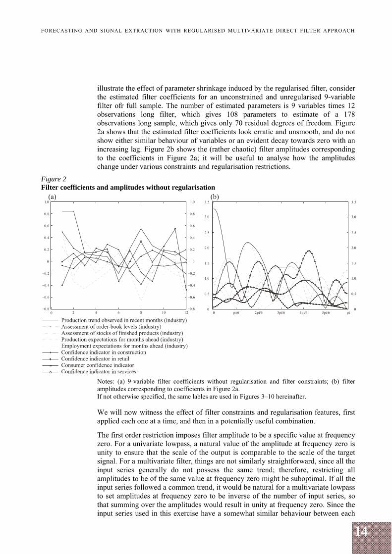
illustrate the effect of parameter shrinkage induced by the regularised filter, consider the estimated filter coefficients for an unconstrained and unregularised 9-variable filter ofr full sample. The number of estimated parameters is 9 variables times 12 observations long filter, which gives 108 parameters to estimate of a 178 observations long sample, which gives only 70 residual degrees of freedom. Figure 2a shows that the estimated filter coefficients look erratic and unsmooth, and do not show either similar behaviour of variables or an evident decay towards zero with an increasing lag. Figure 2b shows the (rather chaotic) filter amplitudes corresponding to the coefficients in Figure 2a; it will be useful to analyse how the amplitudes change under various constraints and regularisation restrictions.
Figure 2 Filter coefficients and amplitudes without regularisation
Notes: (a) 9-variable filter coefficients without regularisation and filter constraints; (b) filter amplitudes corresponding to coefficients in Figure 2a. If not otherwise specified, the same lables are used in Figures 3–10 hereinafter. We will now witness the effect of filter constraints and regularisation features, first applied each one at a time, and then in a potentially useful combination.
The first order restriction imposes filter amplitude to be a specific value at frequency zero. For a univariate lowpass, a natural value of the amplitude at frequency zero is unity to ensure that the scale of the output is comparable to the scale of the target signal. For a multivariate filter, things are not similarly straightforward, since all the input series generally do not possess the same trend; therefore, restricting all amplitudes to be of the same value at frequency zero might be suboptimal. If all the input series followed a common trend, it would be natural for a multivariate lowpass to set amplitudes at frequency zero to be inverse of the number of input series, so that summing over the amplitudes would result in unity at frequency zero. Since the input series used in this exercise have a somewhat similar behaviour between each
15
FORECASTING AND SIGNAL EXTRACTION WITH REGULARISED MULTIVARIATE DIRECT FILTER APPROACH
other, the latter approach is used in this exercise; however, there might be potential gains by using a more sophisticated amplitude constraint that would differentiate amplitude values at frequency zero for different input series; one such approach is discussed in the section below when applying the filter to a higher-dimensional set of explanatory variables.
The first order constraint saves one d.f. per input series, thus nine d.f. are saved for an unregularised nine-variable filter.
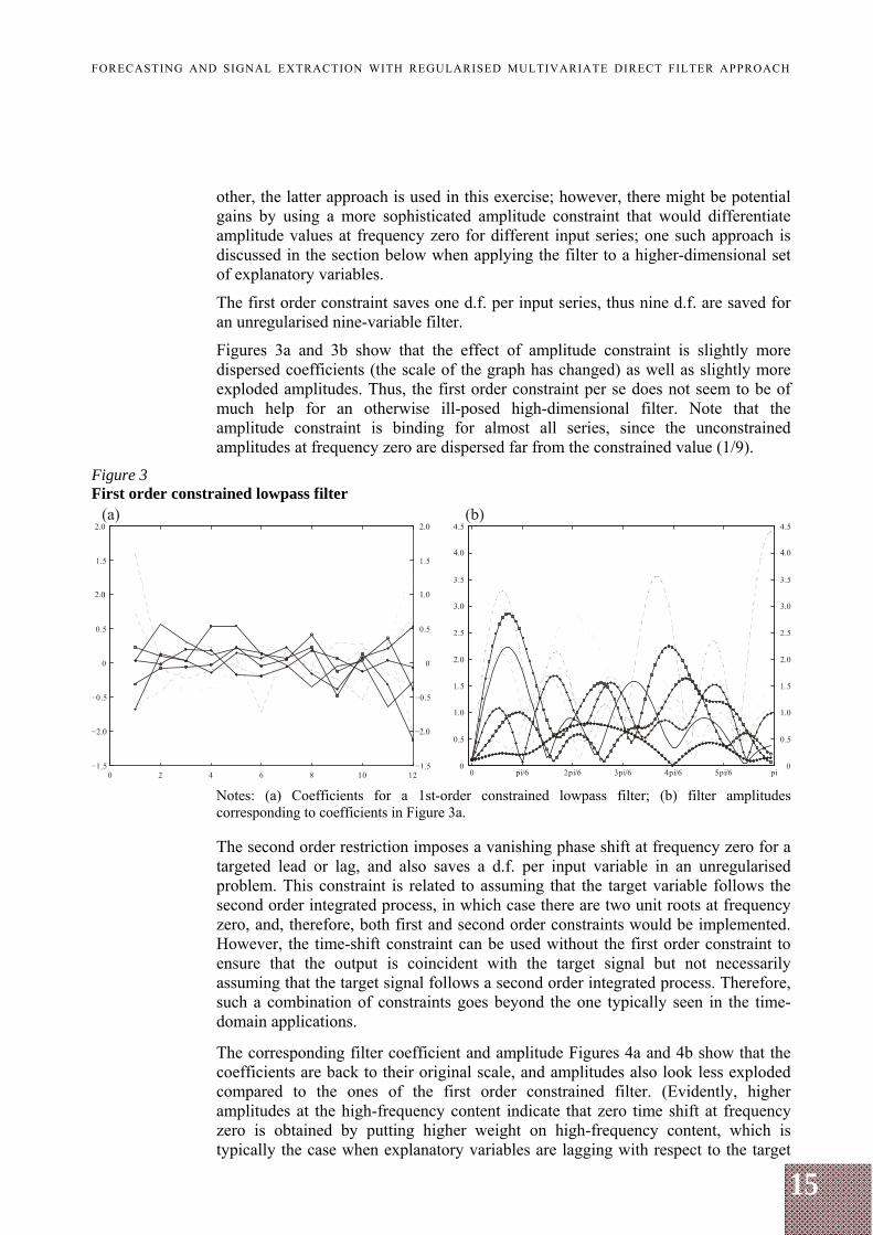
Figures 3a and 3b show that the effect of amplitude constraint is slightly more dispersed coefficients (the scale of the graph has changed) as well as slightly more exploded amplitudes. Thus, the first order constraint per se does not seem to be of much help for an otherwise ill-posed high-dimensional filter. Note that the amplitude constraint is binding for almost all series, since the unconstrained amplitudes at frequency zero are dispersed far from the constrained value (1/9).
Figure 3 First order constrained lowpass filter
Notes: (a) Coefficients for a 1st-order constrained lowpass filter; (b) filter amplitudes corresponding to coefficients in Figure 3a. The second order restriction imposes a vanishing phase shift at frequency zero for a targeted lead or lag, and also saves a d.f. per input variable in an unregularised problem. This constraint is related to assuming that the target variable follows the second order integrated process, in which case there are two unit roots at frequency zero, and, therefore, both first and second order constraints would be implemented. However, the time-shift constraint can be used without the first order constraint to ensure that the output is coincident with the target signal but not necessarily assuming that the target signal follows a second order integrated process. Therefore, such a combination of constraints goes beyond the one typically seen in the time-domain applications.
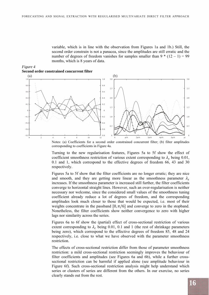
The corresponding filter coefficient and amplitude Figures 4a and 4b show that the coefficients are back to their original scale, and amplitudes also look less exploded compared to the ones of the first order constrained filter. (Evidently, higher amplitudes at the high-frequency content indicate that zero time shift at frequency zero is obtained by putting higher weight on high-frequency content, which is typically the case when explanatory variables are lagging with respect to the target
16
FORECASTING AND SIGNAL EXTRACTION WITH REGULARISED MULTIVARIATE DIRECT FILTER APPROACH
variable, which is in line with the observation from Figures 1a and 1b.) Still, the second order constrain is not a panacea, since the amplitudes are still erratic and the number of degrees of freedom vanishes for samples smaller than 9 * (12 – 1) = 99 months, which is 8 years of data.
Figure 4 Second order constrained concurrent filter
Notes: (a) Coefficients for a second order constrained concurrent filter; (b) filter amplitudes corresponding to coefficients in Figure 4a.
Turning to the new regularisation features, Figures 5a to 5f show the effect of coefficient smoothness restriction of various extent corresponding to being 0.01, 0.1 and 1, which correspond to the effective degrees of freedom 66, 43 and 30 respectively.
Figures 5a to 5f show that the filter coefficients are no longer erratic; they are nice and smooth, and they are getting more linear as the smoothness parameter increases. If the smoothness parameter is increased still further, the filter coefficients converge to horizontal straight lines. However, such an over-regularisation is neither necessary nor welcome, since the considered small values of the smoothness tuning coefficient already reduce a lot of degrees of freedom, and the corresponding amplitudes look much closer to those that would be expected, i.e. most of their weights concentrate in the passband 0, /6 and converge to zero in the stopband. Nonetheless, the filter coefficients show neither convergence to zero with higher lags nor similarity across the series.
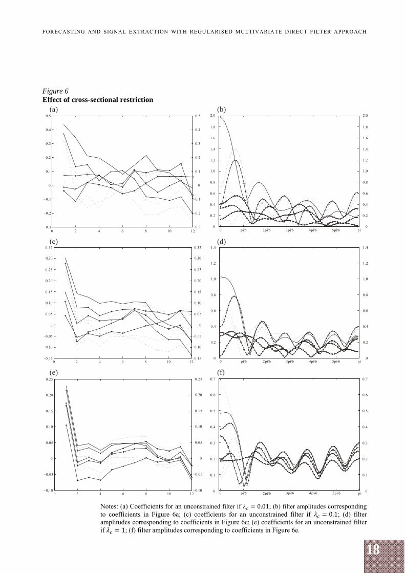
Figures 6a to 6f show the (partial) effect of cross-sectional restriction of various extent corresponding to being 0.01, 0.1 and 1 (the rest of shrinkage parameters being zero), which correspond to the effective degrees of freedom 85, 48 and 24 respectively, i.e. close to what we have observed with the parameter smoothness restriction.
The effects of cross-sectional restriction differ from those of parameter smoothness restriction: a mild cross-sectional restriction seemingly improves the behaviour of filter coefficients and amplitudes (see Figures 6a and 6b), while a further cross-sectional restriction can be harmful if applied alone (see amplitude behaviour in Figure 6f). Such cross-sectional restriction analysis might help understand which series or clusters of series are different from the others. In our exercise, no series clearly stands out from the rest.

17
FORECASTING AND SIGNAL EXTRACTION WITH REGULARISED MULTIVARIATE DIRECT FILTER APPROACH
Figure 5 Effect of coefficient smoothness restriction
Notes: (a) Coefficients for an unconstrained filter if 0.01; (b) filter amplitudes corresponding to coefficients in Figure 5a; (c) coefficients for an unconstrained filter if 0.1; (d) filter amplitudes corresponding to coefficients in Figure 5c; (e) coefficients for an unconstrained filter if 1; (f) filter amplitudes corresponding to coefficients in Figure 5e.
18
FORECASTING AND SIGNAL EXTRACTION WITH REGULARISED MULTIVARIATE DIRECT FILTER APPROACH
Figure 6 Effect of cross-sectional restriction
Notes: (a) Coefficients for an unconstrained filter if 0.01; (b) filter amplitudes corresponding to coefficients in Figure 6a; (c) coefficients for an unconstrained filter if 0.1; (d) filter amplitudes corresponding to coefficients in Figure 6c; (e) coefficients for an unconstrained filter if 1; (f) filter amplitudes corresponding to coefficients in Figure 6e.
19
FORECASTING AND SIGNAL EXTRACTION WITH REGULARISED MULTIVARIATE DIRECT FILTER APPROACH
Figure 7 Effects of longitudinal shrinkage
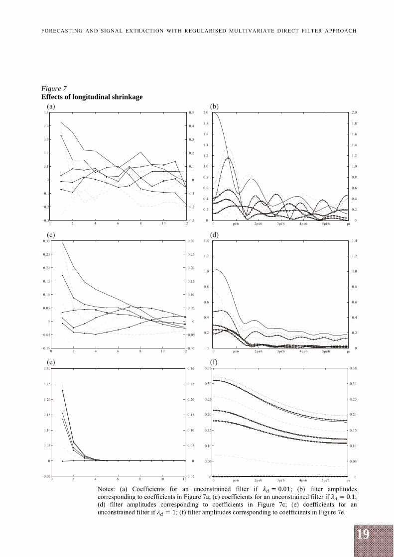
Notes: (a) Coefficients for an unconstrained filter if 0.01; (b) filter amplitudes corresponding to coefficients in Figure 7a; (c) coefficients for an unconstrained filter if 0.1; (d) filter amplitudes corresponding to coefficients in Figure 7c; (e) coefficients for an unconstrained filter if 1; (f) filter amplitudes corresponding to coefficients in Figure 7e.
20
FORECASTING AND SIGNAL EXTRACTION WITH REGULARISED MULTIVARIATE DIRECT FILTER APPROACH
As for the third regularisation feature, Figures 7a to 7f show the effect of longitudinal shrinkage, i.e. a lag decay restriction of various extent corresponding to
being 0.01, 0.1 and 1, which correspond to the effective degrees of freedom 82, 30 and 5 respectively and reflect a stronger shrinkage than we have observed with parameter smoothness or cross-sectional restriction.
Figures 7a to 7f show that a lag decay restriction forces filter coefficients to shrink towards zero as functions of lag, and that a sufficiently high shrinkage parameter yields filter coefficients to be non-zero for a small number of lags. Figure 7 shows that a sufficiently high longitudinal shrinkage forces filter amplitudes to shrink towards zero (see the scale of Figure 7f) and flatten, resembling those of an allpass filter, which is an expected behaviour, since a short filter cannot discriminate between frequencies effectively.
The coefficients in Figure 7c are rather smooth resembling the effect of parameter smoothness restriction. Also, Figure 7 shows that the longitudinal restriction forces filter coefficients to behave somewhat similarly across series, which reminds of the cross-sectional shrinkage. These effects might suggest that the lag decay shrinkage is the most useful of all three shrinkages. Still, the longitudinal shrinkage might conflict, for example, with the parameter smoothness restriction for a sufficiently high lag decay restriction (see Figure 7e). But, instead of using both longitudinal and parameter smoothness regularisation features, one might just loosen the lag decay restriction.
The findings in this paper indeed suggest that the longitudinal shrinkage might be the most useful of the three regularisation features. Moreover, this paper will use only the longitudinal and the cross-sectional shrinkages from the considered regularisation "troika", since the parameter smoothness restriction can be obtained implicitly by the former two.
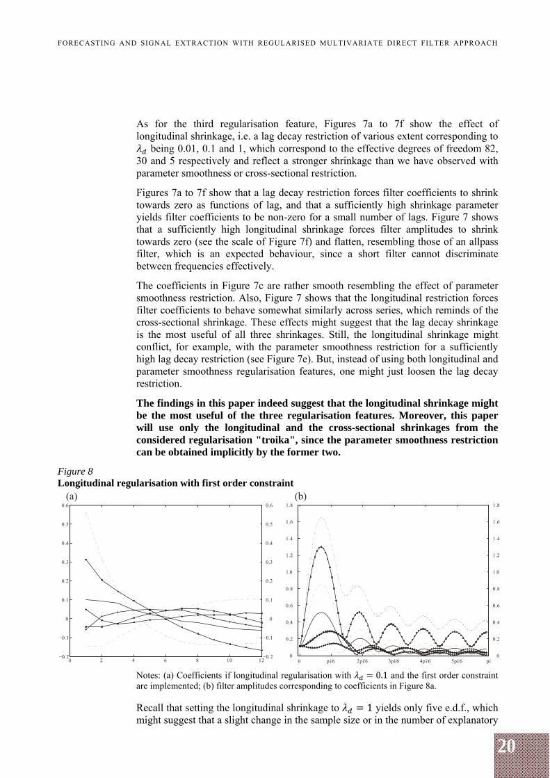
Figure 8 Longitudinal regularisation with first order constraint
Notes: (a) Coefficients if longitudinal regularisation with 0.1 and the first order constraint are implemented; (b) filter amplitudes corresponding to coefficients in Figure 8a. Recall that setting the longitudinal shrinkage to 1 yields only five e.d.f., which might suggest that a slight change in the sample size or in the number of explanatory
21
FORECASTING AND SIGNAL EXTRACTION WITH REGULARISED MULTIVARIATE DIRECT FILTER APPROACH
series could yield close to zero e.d.f. Indeed, the estimation routine can break up if severe regularisation is imposed. Therefore, empirical work should be conducted with caution so that a sufficient number of effective degrees of freedom are given to the estimation routine. Otherwise, the estimation routine will not work not because of overparameterisation but because of "underparameterisation".
Filter constraints have been found to be useful in real-time signal extraction (Bušs (2012)). Therefore, we consider the effect of longitudinal shrinkage combined with either first or second order constraint, or both.
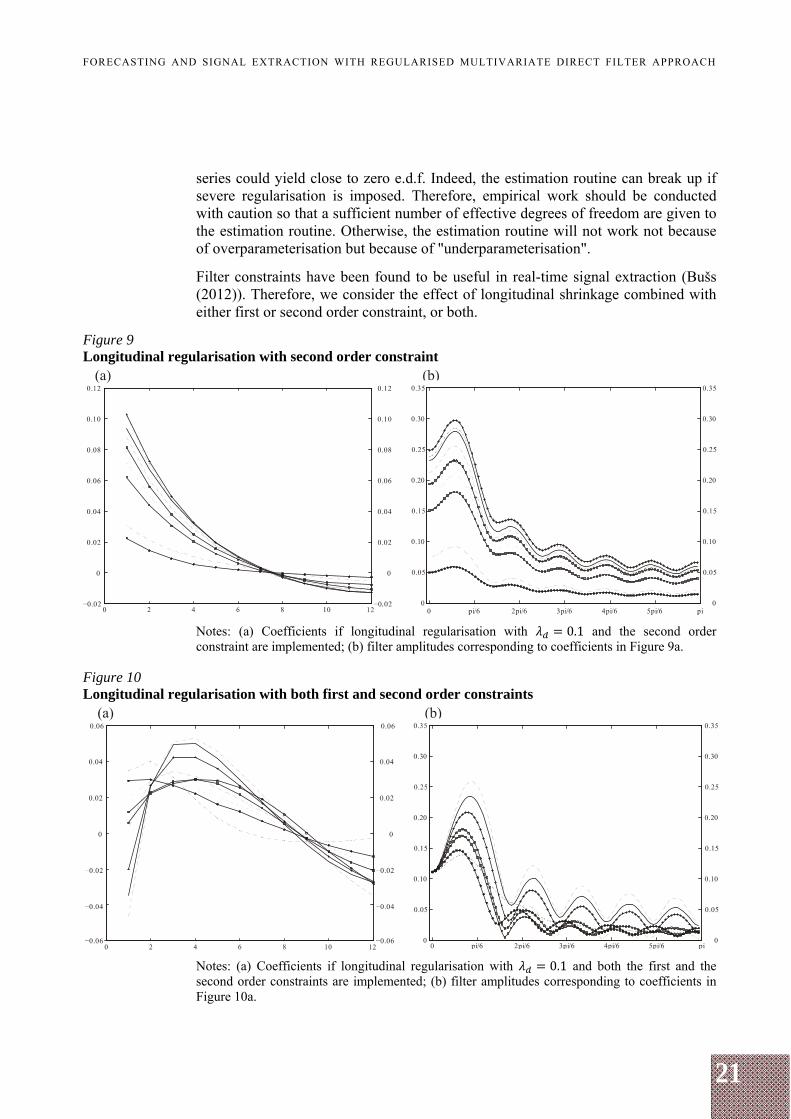
Figure 9 Longitudinal regularisation with second order constraint
Notes: (a) Coefficients if longitudinal regularisation with 0.1 and the second order constraint are implemented; (b) filter amplitudes corresponding to coefficients in Figure 9a.
Figure 10 Longitudinal regularisation with both first and second order constraints
Notes: (a) Coefficients if longitudinal regularisation with 0.1 and both the first and the second order constraints are implemented; (b) filter amplitudes corresponding to coefficients in Figure 10a.
22
FORECASTING AND SIGNAL EXTRACTION WITH REGULARISED MULTIVARIATE DIRECT FILTER APPROACH
Implementation of the first order constraint together with the longitudinal shrinkage yields similarly behaving coefficients and amplitudes whose values at frequency zero are an inverse of the number of input variables, i.e. 1/9. The amplitude values tend to diverge sharply and mostly increase for passband frequencies, afterwards tending to converge and decrease. Instability of the amplitudes at low frequencies might be explained by the restrictive nature of the first order constraint: it forces all amplitudes to be of the same small value, although the unrestricted amplitudes are somewhat dispersed around frequency zero. Also, some of the coefficients are negative at low lags, which can be considered as an unwelcome effect for the dataset where each series correlates positively with the target.
The second order constraint slightly increases the dispersion of coefficients but otherwise does not add drastic changes to the regularised filter.
Implementing both constraints simultaneously is the most restrictive case. Figures 10a and 10b show that the filter coefficients behave more similarly across the series than in the case of no constraint or just the first order constraint (notice the scale of graphs), and so the corresponding amplitudes are less dispersed than in the case of no constraint or just the first order constraint. Still, the negative coefficient values implied by the first order constraint might be considered as somewhat implausible or unwanted, while the cause of their implausibility as restrictive and somewhat arbitrary amplitude constraint. Therefore, if the first order constraint is to be used, one should think of plausible values for amplitudes at frequency zero. Otherwise, instead of using the amplitude constraint, the practitioner might be willing to use the cross-sectional shrinkage as a tool to help controlling for degrees of freedom (at least for rather homogeneous datasets).
2.1.4 Indicator design
The chosen real-time filter design for the yearly growth rate of the EA GDP is thus a regularised, second order constrained lowpass filter with possibly positive longitudinal and cross-sectional shrinkages ( , ) and no parameter smoothness restriction ( ).
Applying the filter to all 72 variables requires more stringent shrinkage. This is done by increasing the longitudinal shrinkage parameter to 0.2 and the cross-sectional shrinkage parameter to 5. The rationale for the chosen shrinkage parameters is as follows. The previous subsection shows that the longitudinal shrinkage is more aggressive than the cross-sectional one. Thus, the longitudinal shrinkage parameter cannot be set too high, since the filter will be effectively too short (filter coefficients will be zero for larger lags). Therefore, in order not to reduce the filter length to an inappropriate value (since a too short filter cannot discriminate between frequencies effectively), the rest of d.f. reduction can be achieved by cross-sectional shrinkage. Increasing the cross-sectional shrinkage parameter to infinity yields filters for all variables to converge, and d.f. to reduce. Thus, increasing the extent of cross-sectional shrinkage does not yield a fatal outcome and, thus, is less harmful than increasing the extent of longitudinal shrinkage. This consideration can be viewed as satisfactory at least for sufficiently homogeneous datasets, which is the case for the EA dataset because it is dominated by a large number of survey data. Indeed, for the EA dataset, increasing the cross-sectional shrinkage parameter to, say, 20, would yield less d.f. but hardly any
23
FORECASTING AND SIGNAL EXTRACTION WITH REGULARISED MULTIVARIATE DIRECT FILTER APPROACH
difference in the filter output. Yet, there is a good reason to allow some d.f. for the filter if the input dataset is heterogeneous.
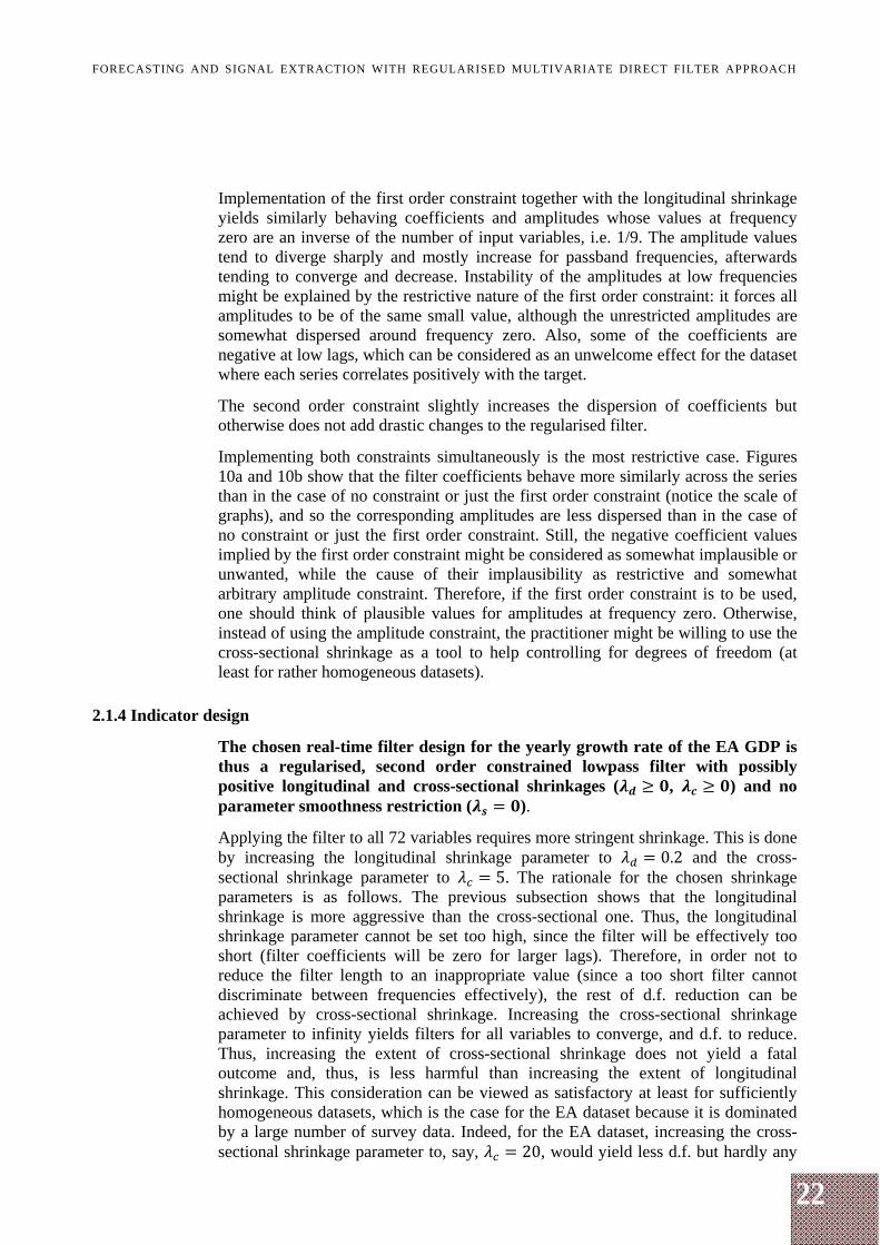
The filter coefficients and amplitudes are shown in Figures 11a and 11b respectively. The figure labels are removed due to over-cluttering.
Figure 11 Concurrent 72-variable filter with second order constraint, , . ,
Notes: (a) Coefficients for concurrent 72-variable filter with second order constraint, 0, 0.2, 5; (b) filter amplitudes corresponding to coefficients in Figure 11a.
The resulting filter coefficients and amplitudes look plausible. The coefficients for small lags are positive and decay smoothly to zero with a higher lag order. Filters with coefficients that do not shrink to zero at higher lag orders can be argued to be suboptimal or incomplete. The amplitudes also look plausible: there is some d.f. so that they are not the same for all variables but they are still close to each other, have the most weight in the passband, and decay towards zero in the stopband.
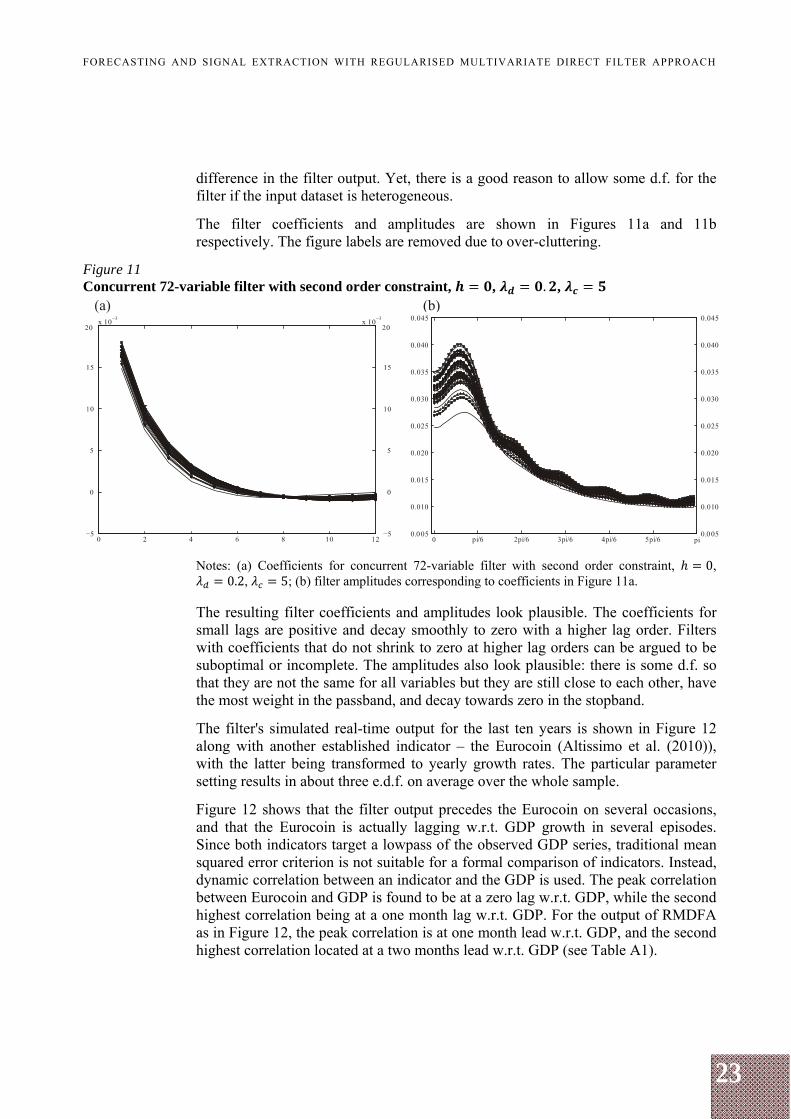
The filter's simulated real-time output for the last ten years is shown in Figure 12 along with another established indicator – the Eurocoin (Altissimo et al. (2010)), with the latter being transformed to yearly growth rates. The particular parameter setting results in about three e.d.f. on average over the whole sample.
Figure 12 shows that the filter output precedes the Eurocoin on several occasions, and that the Eurocoin is actually lagging w.r.t. GDP growth in several episodes. Since both indicators target a lowpass of the observed GDP series, traditional mean squared error criterion is not suitable for a formal comparison of indicators. Instead, dynamic correlation between an indicator and the GDP is used. The peak correlation between Eurocoin and GDP is found to be at a zero lag w.r.t. GDP, while the second highest correlation being at a one month lag w.r.t. GDP. For the output of RMDFA as in Figure 12, the peak correlation is at one month lead w.r.t. GDP, and the second highest correlation located at a two months lead w.r.t. GDP (see Table A1).
24
FORECASTING AND SIGNAL EXTRACTION WITH REGULARISED MULTIVARIATE DIRECT FILTER APPROACH
Figure 12 Output of regularised 72-variable filter with , . ,
Note: Output of the filter tracking trendcycle in y-o-y EA GDP versus Eurocoin transformed to represent yearly growth rates.
Forecasting
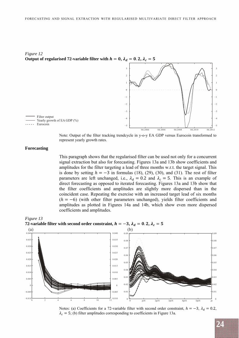
This paragraph shows that the regularised filter can be used not only for a concurrent signal extraction but also for forecasting. Figures 13a and 13b show coefficients and amplitudes for the filter targeting a lead of three months w.r.t. the target signal. This is done by setting 3 in formulas (18), (29), (30), and (31). The rest of filter parameters are left unchanged, i.e., 0.2 and 5. This is an example of direct forecasting as opposed to iterated forecasting. Figures 13a and 13b show that the filter coefficients and amplitudes are slightly more dispersed than in the coincident case. Repeating the exercise with an increased target lead of six months ( 6) (with other filter parameters unchanged), yields filter coefficients and amplitudes as plotted in Figures 14a and 14b, which show even more dispersed coefficients and amplitudes.
Figure 13 72-variable filter with second order constraint, , . ,
Notes: (a) Coefficients for a 72-variable filter with second order constraint, 3, 0.2, 5; (b) filter amplitudes corresponding to coefficients in Figure 13a.
25
FORECASTING AND SIGNAL EXTRACTION WITH REGULARISED MULTIVARIATE DIRECT FILTER APPROACH
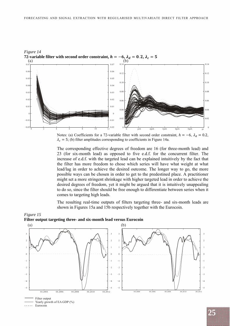
Figure 14 72-variable filter with second order constraint, , . ,
Notes: (a) Coefficients for a 72-variable filter with second order constraint, 6, 0.2, 5; (b) filter amplitudes corresponding to coefficients in Figure 14a.
The corresponding effective degrees of freedom are 16 (for three-month lead) and 23 (for six-month lead) as opposed to five e.d.f. for the concurrent filter. The increase of e.d.f. with the targeted lead can be explained intuitively by the fact that the filter has more freedom to chose which series will have what weight at what lead/lag in order to achieve the desired outcome. The longer way to go, the more possible ways can be chosen in order to get to the predestined place. A practitioner might set a more stringent shrinkage with higher targeted lead in order to achieve the desired degrees of freedom, yet it might be argued that it is intuitively unappealing to do so, since the filter should be free enough to differentiate between series when it comes to targeting high leads.
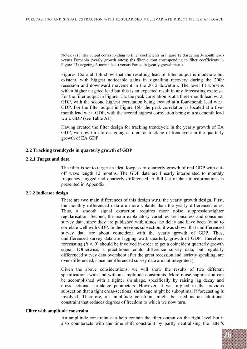
The resulting real-time outputs of filters targeting three- and six-month leads are shown in Figures 15a and 15b respectively together with the Eurocoin.
Figure 15 Filter output targeting three- and six-month lead versus Eurocoin
26
FORECASTING AND SIGNAL EXTRACTION WITH REGULARISED MULTIVARIATE DIRECT FILTER APPROACH
Notes: (a) Filter output corresponding to filter coefficients in Figure 12 (targeting 3-month lead) versus Eurocoin (yearly growth rates); (b) filter output corresponding to filter coefficients in Figure 13 (targeting 6-month lead) versus Eurocoin (yearly growth rates). Figures 15a and 15b show that the resulting lead of filter output is moderate but existent, with biggest noticeable gains in signalling recovery during the 2009 recession and downward movement in the 2012 downturn. The level fit worsens with a higher targeted lead but this is an expected result in any forecasting exercise. For the filter output in Figure 15a, the peak correlation is at a three-month lead w.r.t. GDP, with the second highest correlation being located at a four-month lead w.r.t. GDP. For the filter output in Figure 15b, the peak correlation is located at a five-month lead w.r.t. GDP, with the second highest correlation being at a six-month lead w.r.t. GDP (see Table A1).
Having created the filter design for tracking trendcycle in the yearly growth of EA GDP, we now turn to designing a filter for tracking of trendcycle in the quarterly growth of EA GDP.
2.2 Tracking trendcycle in quarterly growth of GDP
2.2.1 Target and data
The filter is set to target an ideal lowpass of quarterly growth of real GDP with cut-off wave length 12 months. The GDP data are linearly interpolated to monthly frequency, logged and quarterly differenced. A full list of data transformations is presented in Appendix.
2.2.2 Indicator design
There are two main differences of this design w.r.t. the yearly growth design. First, the monthly differenced data are more volatile than the yearly differenced ones. Thus, a smooth signal extraction requires more noise suppression/tighter regularisation. Second, the main explanatory variables are business and consumer survey data, since they are published with almost no delay and have been found to correlate well with GDP. In the previous subsection, it was shown that undifferenced survey data are about coincident with the yearly growth of GDP. Thus, undifferenced survey data are lagging w.r.t. quarterly growth of GDP. Therefore, forecasting ( 0) should be involved in order to get a coincident quarterly growth signal. (Otherwise, a practitioner could difference survey data, but regularly differenced survey data overshoot after the great recession and, strictly speaking, are over-differenced, since undifferenced survey data are not integrated.)
Given the above considerations, we will show the results of two different specifications with and without amplitude constraints. More noise suppression can be accomplished with a tighter shrinkage, specifically by raising lag decay and cross-sectional shrinkage parameters. However, it was argued in the previous subsection that a tight cross-sectional shrinkage might be suboptimal if forecasting is involved. Therefore, an amplitude constraint might be used as an additional constraint that reduces degrees of freedom to which we now turn.
Filter with amplitude constraint
An amplitude constraint can help contain the filter output on the right level but it also counteracts with the time shift constraint by partly neutralising the latter's
27
FORECASTING AND SIGNAL EXTRACTION WITH REGULARISED MULTIVARIATE DIRECT FILTER APPROACH
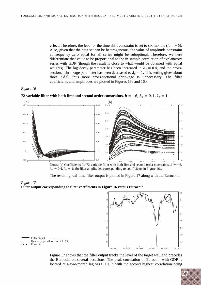
effect. Therefore, the lead for the time shift constraint is set to six months ( 6). Also, given that the data set can be heterogeneous, the value of amplitude constraint at frequency zero equal for all series might be suboptimal. Therefore, we here differentiate that value to be proportional to the in-sample correlation of explanatory series with GDP (though the result is close to what would be obtained with equal weights). The lag decay parameter has been increased to 0.4, and the cross-sectional shrinkage parameter has been decreased to 1. This setting gives about three e.d.f., thus more cross-sectional shrinkage is unnecessary. The filter coefficients and amplitudes are plotted in Figures 16a and 16b.
Figure 16
72-variable filter with both first and second order constraints, , . ,
Notes: (a) Coefficients for 72-variable filter with both first and second order constraints, 6,
0.4, 1; (b) filter amplitudes corresponding to coefficients in Figure 16a.
The resulting real-time filter output is plotted in Figure 17 along with the Eurocoin.
Figure 17 Filter output corresponding to filter coefficients in Figure 16 versus Eurocoin
Figure 17 shows that the filter output tracks the level of the target well and precedes the Eurocoin on several occasions. The peak correlation of Eurocoin with GDP is located at a two-month lag w.r.t. GDP, with the second highest correlation being
28
FORECASTING AND SIGNAL EXTRACTION WITH REGULARISED MULTIVARIATE DIRECT FILTER APPROACH
located at a one-month lag w.r.t. GDP. For the RMDFA output in Figure 17, the peak correlation is located at a one-month lag w.r.t. GDP, with the second highest correlation being at a zero-month lag w.r.t. GDP (see Table A1).
Note that the true real-time performance of Eurocoin begins in mid-2009; after that period, the difference between the performance of the two indicators is slightly more evident.
Filter without amplitude constraint
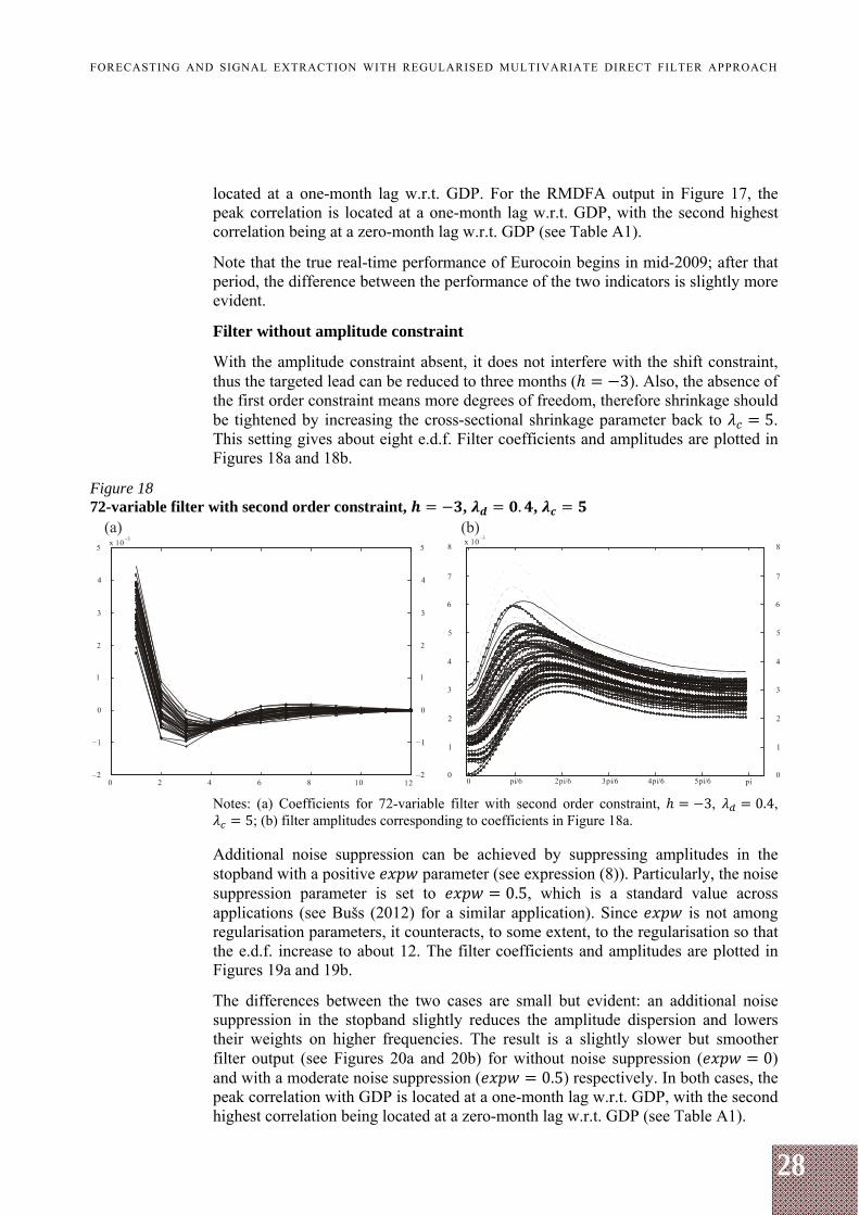
With the amplitude constraint absent, it does not interfere with the shift constraint, thus the targeted lead can be reduced to three months ( 3). Also, the absence of the first order constraint means more degrees of freedom, therefore shrinkage should be tightened by increasing the cross-sectional shrinkage parameter back to 5. This setting gives about eight e.d.f. Filter coefficients and amplitudes are plotted in Figures 18a and 18b.
Figure 18 72-variable filter with second order constraint, , . ,
Notes: (a) Coefficients for 72-variable filter with second order constraint, 3, 0.4, 5; (b) filter amplitudes corresponding to coefficients in Figure 18a.
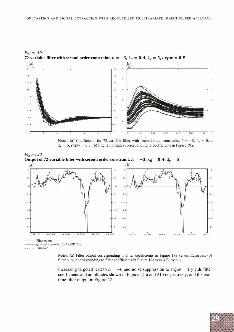
Additional noise suppression can be achieved by suppressing amplitudes in the stopband with a positive parameter (see expression (8)). Particularly, the noise suppression parameter is set to 0.5, which is a standard value across applications (see Bušs (2012) for a similar application). Since is not among regularisation parameters, it counteracts, to some extent, to the regularisation so that the e.d.f. increase to about 12. The filter coefficients and amplitudes are plotted in Figures 19a and 19b.
The differences between the two cases are small but evident: an additional noise suppression in the stopband slightly reduces the amplitude dispersion and lowers their weights on higher frequencies. The result is a slightly slower but smoother filter output (see Figures 20a and 20b) for without noise suppression ( 0) and with a moderate noise suppression ( 0.5) respectively. In both cases, the peak correlation with GDP is located at a one-month lag w.r.t. GDP, with the second highest correlation being located at a zero-month lag w.r.t. GDP (see Table A1).
29
FORECASTING AND SIGNAL EXTRACTION WITH REGULARISED MULTIVARIATE DIRECT FILTER APPROACH
Figure 19 72-variable filter with second order constraint, , . , , .
Notes: (a) Coefficients for 72-variable filter with second order constraint, 3, 0.4, 5, 0.5; (b) filter amplitudes corresponding to coefficients in Figure 19a.
Figure 20 Output of 72-variable filter with second order constraint, , . ,
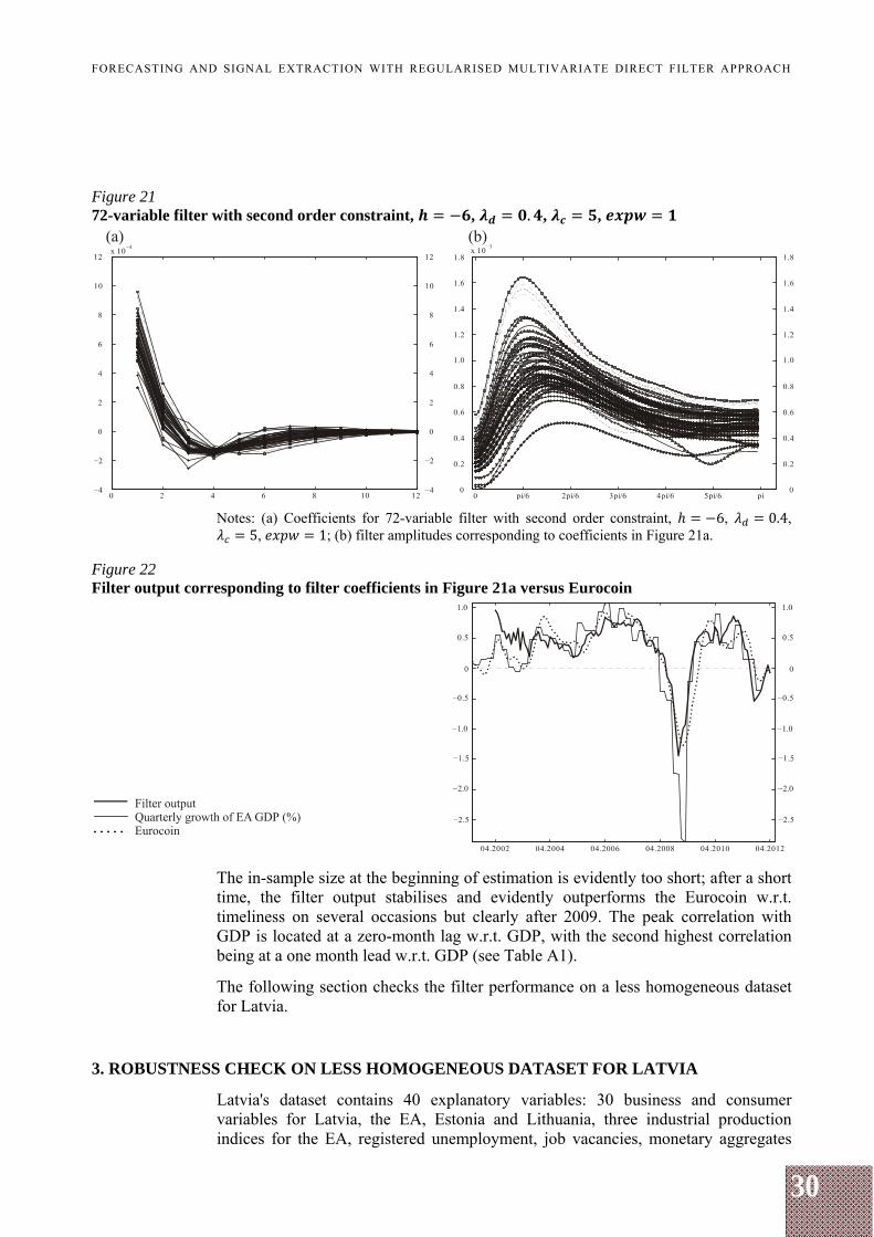
Notes: (a) Filter output corresponding to filter coefficients in Figure 18a versus Eurocoin; (b) filter output corresponding to filter coefficients in Figure 19a versus Eurocoin. Increasing targeted lead to 6 and noise suppression to 1 yields filter coefficients and amplitudes shown in Figures 21a and 21b respectively, and the real-time filter output in Figure 22.
30
FORECASTING AND SIGNAL EXTRACTION WITH REGULARISED MULTIVARIATE DIRECT FILTER APPROACH
Figure 21 72-variable filter with second order constraint, , . , ,
Notes: (a) Coefficients for 72-variable filter with second order constraint, 6, 0.4, 5, 1; (b) filter amplitudes corresponding to coefficients in Figure 21a.
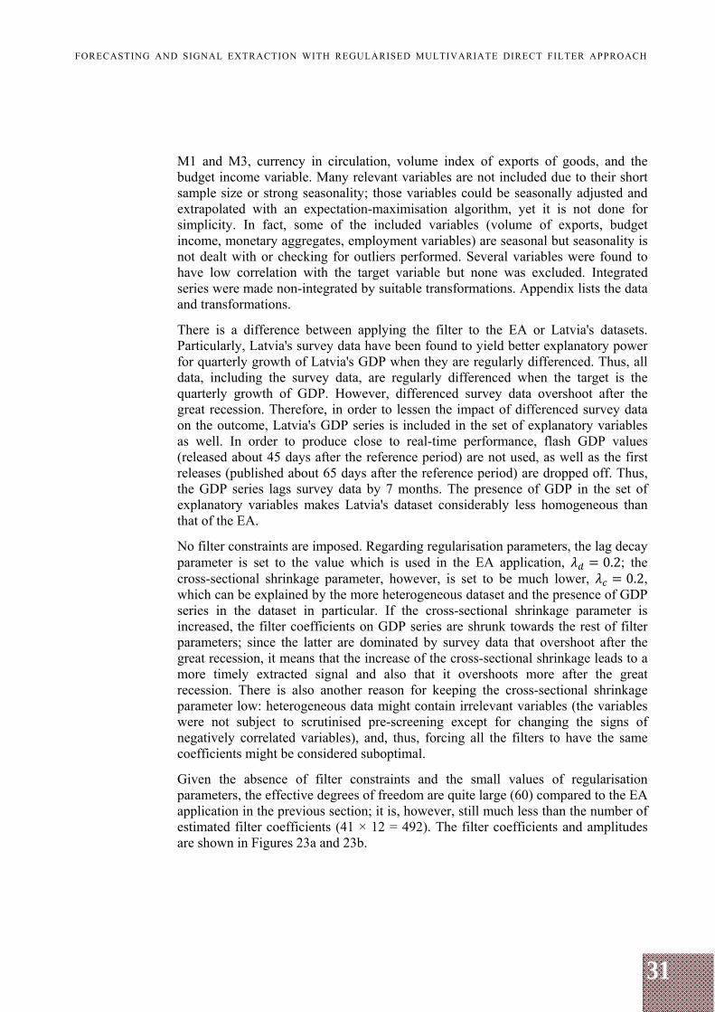
Figure 22 Filter output corresponding to filter coefficients in Figure 21a versus Eurocoin
The in-sample size at the beginning of estimation is evidently too short; after a short time, the filter output stabilises and evidently outperforms the Eurocoin w.r.t. timeliness on several occasions but clearly after 2009. The peak correlation with GDP is located at a zero-month lag w.r.t. GDP, with the second highest correlation being at a one month lead w.r.t. GDP (see Table A1).
The following section checks the filter performance on a less homogeneous dataset for Latvia.
3. ROBUSTNESS CHECK ON LESS HOMOGENEOUS DATASET FOR LATVIA
Latvia's dataset contains 40 explanatory variables: 30 business and consumer variables for Latvia, the EA, Estonia and Lithuania, three industrial production indices for the EA, registered unemployment, job vacancies, monetary aggregates
31
FORECASTING AND SIGNAL EXTRACTION WITH REGULARISED MULTIVARIATE DIRECT FILTER APPROACH
M1 and M3, currency in circulation, volume index of exports of goods, and the budget income variable. Many relevant variables are not included due to their short sample size or strong seasonality; those variables could be seasonally adjusted and extrapolated with an expectation-maximisation algorithm, yet it is not done for simplicity. In fact, some of the included variables (volume of exports, budget income, monetary aggregates, employment variables) are seasonal but seasonality is not dealt with or checking for outliers performed. Several variables were found to have low correlation with the target variable but none was excluded. Integrated series were made non-integrated by suitable transformations. Appendix lists the data and transformations.
There is a difference between applying the filter to the EA or Latvia's datasets. Particularly, Latvia's survey data have been found to yield better explanatory power for quarterly growth of Latvia's GDP when they are regularly differenced. Thus, all data, including the survey data, are regularly differenced when the target is the quarterly growth of GDP. However, differenced survey data overshoot after the great recession. Therefore, in order to lessen the impact of differenced survey data on the outcome, Latvia's GDP series is included in the set of explanatory variables as well. In order to produce close to real-time performance, flash GDP values (released about 45 days after the reference period) are not used, as well as the first releases (published about 65 days after the reference period) are dropped off. Thus, the GDP series lags survey data by 7 months. The presence of GDP in the set of explanatory variables makes Latvia's dataset considerably less homogeneous than that of the EA.
No filter constraints are imposed. Regarding regularisation parameters, the lag decay parameter is set to the value which is used in the EA application, 0.2; the cross-sectional shrinkage parameter, however, is set to be much lower, 0.2, which can be explained by the more heterogeneous dataset and the presence of GDP series in the dataset in particular. If the cross-sectional shrinkage parameter is increased, the filter coefficients on GDP series are shrunk towards the rest of filter parameters; since the latter are dominated by survey data that overshoot after the great recession, it means that the increase of the cross-sectional shrinkage leads to a more timely extracted signal and also that it overshoots more after the great recession. There is also another reason for keeping the cross-sectional shrinkage parameter low: heterogeneous data might contain irrelevant variables (the variables were not subject to scrutinised pre-screening except for changing the signs of negatively correlated variables), and, thus, forcing all the filters to have the same coefficients might be considered suboptimal.
Given the absence of filter constraints and the small values of regularisation parameters, the effective degrees of freedom are quite large (60) compared to the EA application in the previous section; it is, however, still much less than the number of estimated filter coefficients (41 × 12 = 492). The filter coefficients and amplitudes are shown in Figures 23a and 23b.
32
FORECASTING AND SIGNAL EXTRACTION WITH REGULARISED MULTIVARIATE DIRECT FILTER APPROACH
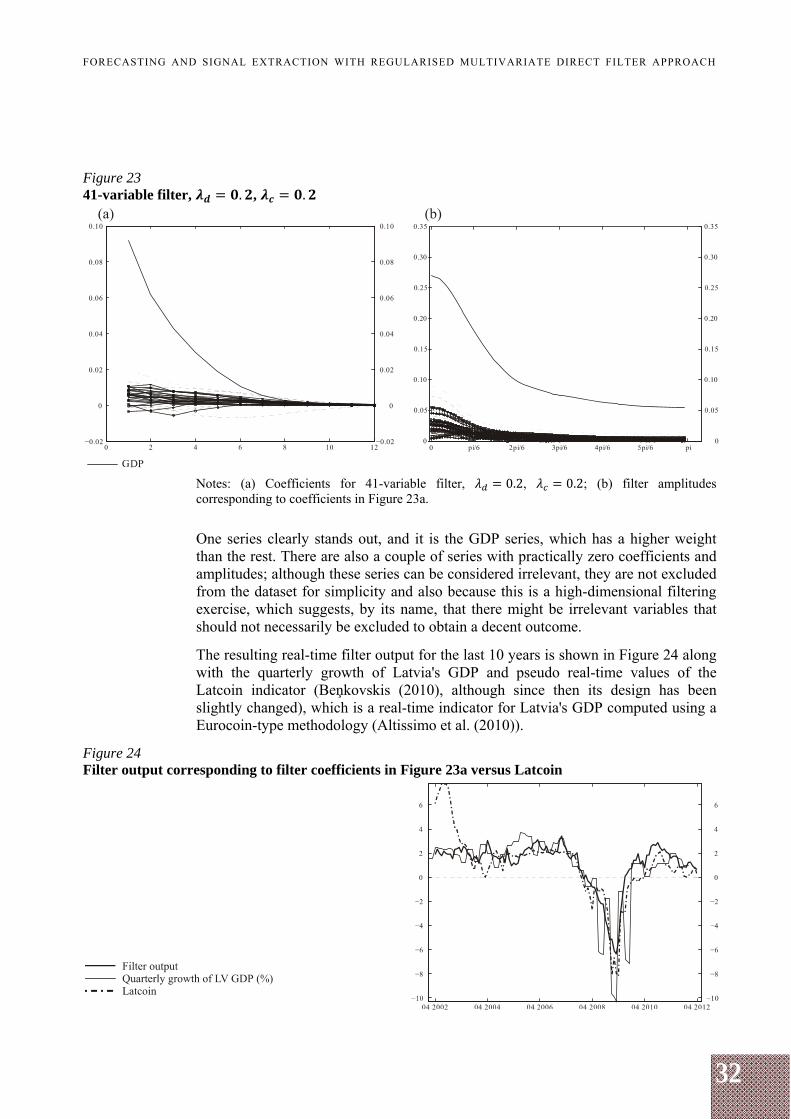
Figure 23 41-variable filter, . , .
Notes: (a) Coefficients for 41-variable filter, 0.2, 0.2; (b) filter amplitudes corresponding to coefficients in Figure 23a.
One series clearly stands out, and it is the GDP series, which has a higher weight than the rest. There are also a couple of series with practically zero coefficients and amplitudes; although these series can be considered irrelevant, they are not excluded from the dataset for simplicity and also because this is a high-dimensional filtering exercise, which suggests, by its name, that there might be irrelevant variables that should not necessarily be excluded to obtain a decent outcome.
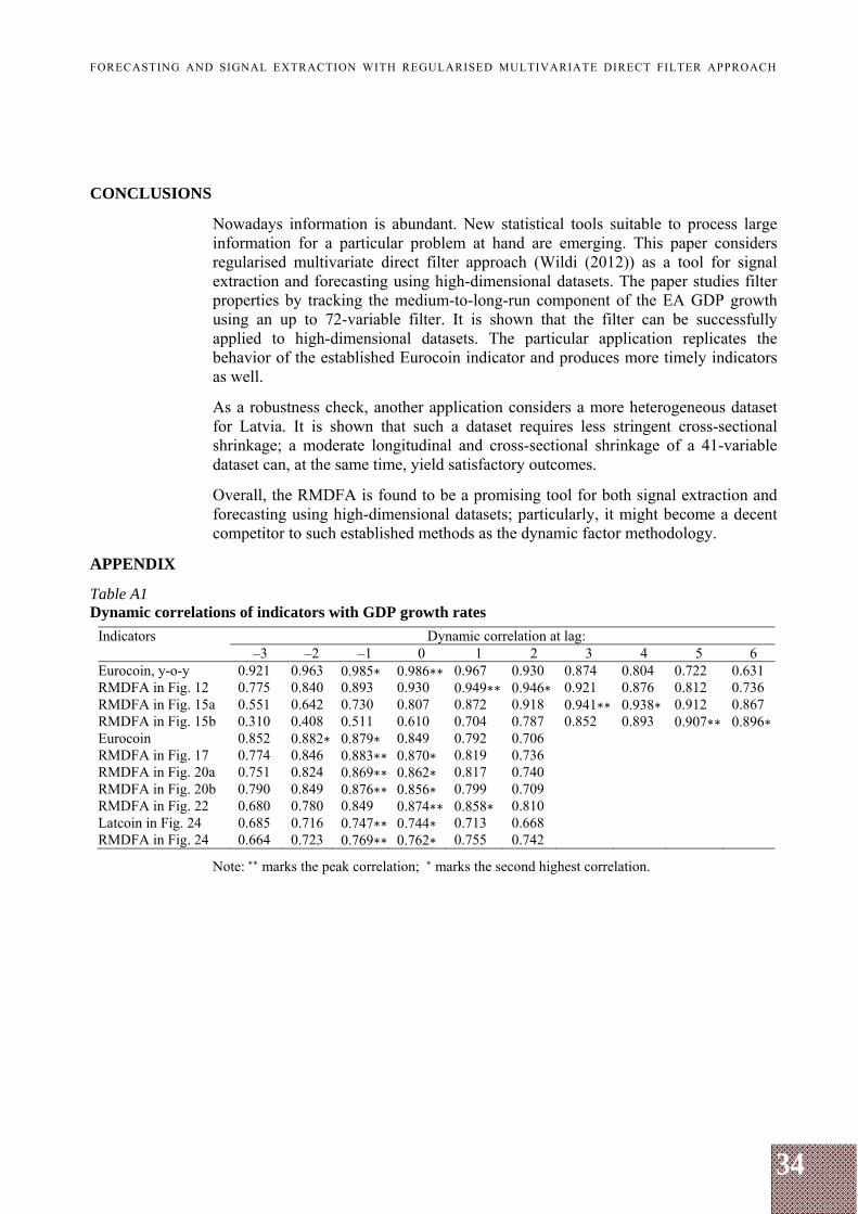
The resulting real-time filter output for the last 10 years is shown in Figure 24 along with the quarterly growth of Latvia's GDP and pseudo real-time values of the Latcoin indicator (Beņkovskis (2010), although since then its design has been slightly changed), which is a real-time indicator for Latvia's GDP computed using a Eurocoin-type methodology (Altissimo et al. (2010)).
Figure 24 Filter output corresponding to filter coefficients in Figure 23a versus Latcoin

33
FORECASTING AND SIGNAL EXTRACTION WITH REGULARISED MULTIVARIATE DIRECT FILTER APPROACH
Figure 24 shows that the filter output is almost coincident with the Latcoin yet smoother during the great recession period and slightly faster during the recovery phase. It also appears to be more robust for smaller samples despite more parameters contained. The peak correlations indicate that both indicators are almost coincident with GDP (see Table A1).
34
FORECASTING AND SIGNAL EXTRACTION WITH REGULARISED MULTIVARIATE DIRECT FILTER APPROACH
CONCLUSIONS
Nowadays information is abundant. New statistical tools suitable to process large information for a particular problem at hand are emerging. This paper considers regularised multivariate direct filter approach (Wildi (2012)) as a tool for signal extraction and forecasting using high-dimensional datasets. The paper studies filter properties by tracking the medium-to-long-run component of the EA GDP growth using an up to 72-variable filter. It is shown that the filter can be successfully applied to high-dimensional datasets. The particular application replicates the behavior of the established Eurocoin indicator and produces more timely indicators as well.
As a robustness check, another application considers a more heterogeneous dataset for Latvia. It is shown that such a dataset requires less stringent cross-sectional shrinkage; a moderate longitudinal and cross-sectional shrinkage of a 41-variable dataset can, at the same time, yield satisfactory outcomes.
Overall, the RMDFA is found to be a promising tool for both signal extraction and forecasting using high-dimensional datasets; particularly, it might become a decent competitor to such established methods as the dynamic factor methodology.
APPENDIX
Table A1 Dynamic correlations of indicators with GDP growth rates
Indicators Dynamic correlation at lag: –3 –2 –1 0 1 2 3 4 5 6
Eurocoin, y-o-y 0.921 0.963 0.985∗ 0.986∗∗ 0.967 0.930 0.874 0.804 0.722 0.631 RMDFA in Fig. 12 0.775 0.840 0.893 0.930 0.949∗∗ 0.946∗ 0.921 0.876 0.812 0.736 RMDFA in Fig. 15a 0.551 0.642 0.730 0.807 0.872 0.918 0.941∗∗ 0.938∗ 0.912 0.867 RMDFA in Fig. 15b 0.310 0.408 0.511 0.610 0.704 0.787 0.852 0.893 0.907∗∗ 0.896∗Eurocoin 0.852 0.882∗ 0.879∗ 0.849 0.792 0.706 RMDFA in Fig. 17 0.774 0.846 0.883∗∗ 0.870∗ 0.819 0.736 RMDFA in Fig. 20a 0.751 0.824 0.869∗∗ 0.862∗ 0.817 0.740 RMDFA in Fig. 20b 0.790 0.849 0.876∗∗ 0.856∗ 0.799 0.709 RMDFA in Fig. 22 0.680 0.780 0.849 0.874∗∗ 0.858∗ 0.810 Latcoin in Fig. 24 0.685 0.716 0.747∗∗ 0.744∗ 0.713 0.668 RMDFA in Fig. 24 0.664 0.723 0.769∗∗ 0.762∗ 0.755 0.742
Note:∗∗ marks the peak correlation; ∗ marks the second highest correlation.
35
FORECASTING AND SIGNAL EXTRACTION WITH REGULARISED MULTIVARIATE DIRECT FILTER APPROACH
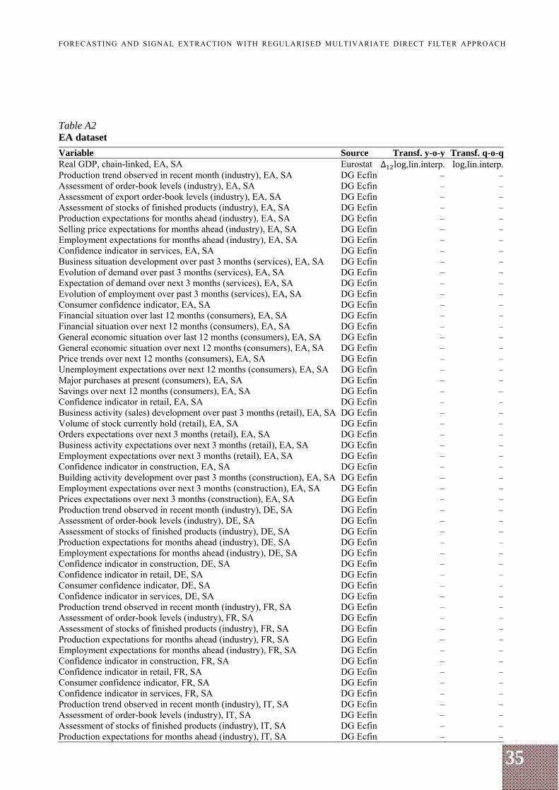
Table A2 EA dataset
Variable Source Transf. y-o-y Transf. q-o-q Real GDP, chain-linked, EA, SA Eurostat Δ log,lin.interp. log,lin.interp. Production trend observed in recent month (industry), EA, SA DG Ecfin – –Assessment of order-book levels (industry), EA, SA DG Ecfin – –Assessment of export order-book levels (industry), EA, SA DG Ecfin – –Assessment of stocks of finished products (industry), EA, SA DG Ecfin – –Production expectations for months ahead (industry), EA, SA DG Ecfin – –Selling price expectations for months ahead (industry), EA, SA DG Ecfin – –Employment expectations for months ahead (industry), EA, SA DG Ecfin – –Confidence indicator in services, EA, SA DG Ecfin – –Business situation development over past 3 months (services), EA, SA DG Ecfin – –Evolution of demand over past 3 months (services), EA, SA DG Ecfin – –Expectation of demand over next 3 months (services), EA, SA DG Ecfin – –Evolution of employment over past 3 months (services), EA, SA DG Ecfin – –Consumer confidence indicator, EA, SA DG Ecfin – –Financial situation over last 12 months (consumers), EA, SA DG Ecfin – –Financial situation over next 12 months (consumers), EA, SA DG Ecfin – –General economic situation over last 12 months (consumers), EA, SA DG Ecfin – –General economic situation over next 12 months (consumers), EA, SA DG Ecfin – –Price trends over next 12 months (consumers), EA, SA DG Ecfin – –Unemployment expectations over next 12 months (consumers), EA, SA DG Ecfin – –Major purchases at present (consumers), EA, SA DG Ecfin – –Savings over next 12 months (consumers), EA, SA DG Ecfin – –Confidence indicator in retail, EA, SA DG Ecfin – –Business activity (sales) development over past 3 months (retail), EA, SA DG Ecfin – –Volume of stock currently hold (retail), EA, SA DG Ecfin – –Orders expectations over next 3 months (retail), EA, SA DG Ecfin – –Business activity expectations over next 3 months (retail), EA, SA DG Ecfin – –Employment expectations over next 3 months (retail), EA, SA DG Ecfin – –Confidence indicator in construction, EA, SA DG Ecfin – –Building activity development over past 3 months (construction), EA, SA DG Ecfin – –Employment expectations over next 3 months (construction), EA, SA DG Ecfin – –Prices expectations over next 3 months (construction), EA, SA DG Ecfin – –Production trend observed in recent month (industry), DE, SA DG Ecfin – –Assessment of order-book levels (industry), DE, SA DG Ecfin – –Assessment of stocks of finished products (industry), DE, SA DG Ecfin – –Production expectations for months ahead (industry), DE, SA DG Ecfin – –Employment expectations for months ahead (industry), DE, SA DG Ecfin – –Confidence indicator in construction, DE, SA DG Ecfin – –Confidence indicator in retail, DE, SA DG Ecfin – –Consumer confidence indicator, DE, SA DG Ecfin – –Confidence indicator in services, DE, SA DG Ecfin – –Production trend observed in recent month (industry), FR, SA DG Ecfin – –Assessment of order-book levels (industry), FR, SA DG Ecfin – –Assessment of stocks of finished products (industry), FR, SA DG Ecfin – –Production expectations for months ahead (industry), FR, SA DG Ecfin – –Employment expectations for months ahead (industry), FR, SA DG Ecfin – –Confidence indicator in construction, FR, SA DG Ecfin – –Confidence indicator in retail, FR, SA DG Ecfin – –Consumer confidence indicator, FR, SA DG Ecfin – –Confidence indicator in services, FR, SA DG Ecfin – –Production trend observed in recent month (industry), IT, SA DG Ecfin – –Assessment of order-book levels (industry), IT, SA DG Ecfin – –Assessment of stocks of finished products (industry), IT, SA DG Ecfin – –Production expectations for months ahead (industry), IT, SA DG Ecfin – –
36
FORECASTING AND SIGNAL EXTRACTION WITH REGULARISED MULTIVARIATE DIRECT FILTER APPROACH
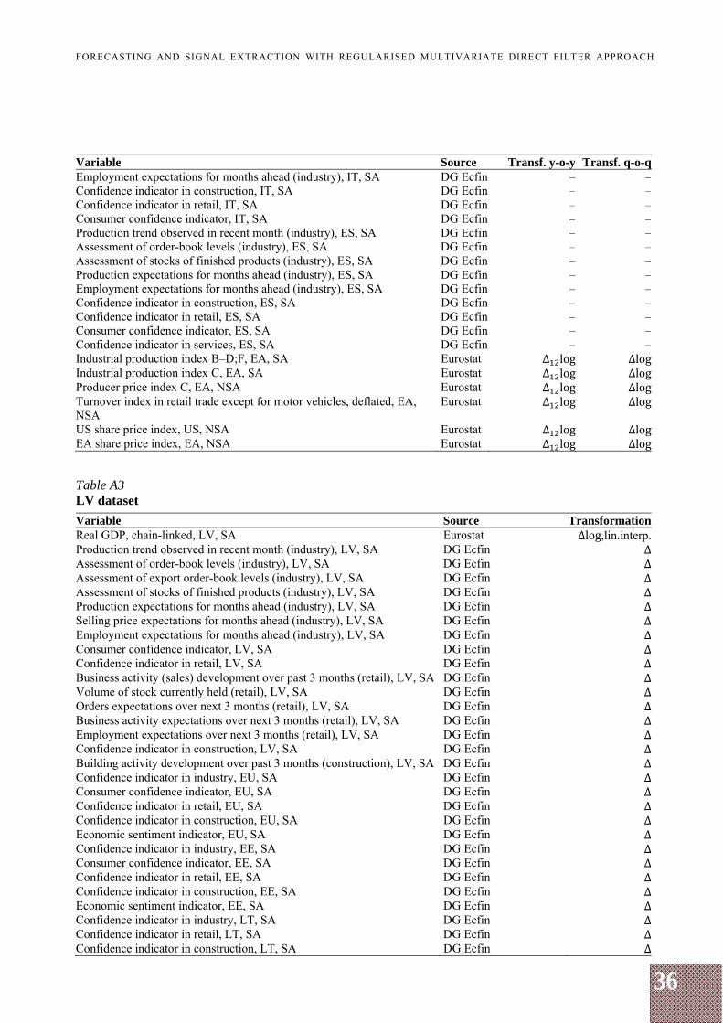
Variable Source Transf. y-o-y Transf. q-o-q Employment expectations for months ahead (industry), IT, SA DG Ecfin – –Confidence indicator in construction, IT, SA DG Ecfin – –Confidence indicator in retail, IT, SA DG Ecfin – –Consumer confidence indicator, IT, SA DG Ecfin – –Production trend observed in recent month (industry), ES, SA DG Ecfin – –Assessment of order-book levels (industry), ES, SA DG Ecfin – –Assessment of stocks of finished products (industry), ES, SA DG Ecfin – –Production expectations for months ahead (industry), ES, SA DG Ecfin – –Employment expectations for months ahead (industry), ES, SA DG Ecfin – –Confidence indicator in construction, ES, SA DG Ecfin – –Confidence indicator in retail, ES, SA DG Ecfin – –Consumer confidence indicator, ES, SA DG Ecfin – –Confidence indicator in services, ES, SA DG Ecfin – –Industrial production index B–D;F, EA, SA Eurostat Δ log ΔlogIndustrial production index C, EA, SA Eurostat Δ log ΔlogProducer price index C, EA, NSA Eurostat Δ log ΔlogTurnover index in retail trade except for motor vehicles, deflated, EA, NSA
Eurostat Δ log Δlog
US share price index, US, NSA Eurostat Δ log ΔlogEA share price index, EA, NSA Eurostat Δ log Δlog
Table A3 LV dataset
Variable Source Transformation Real GDP, chain-linked, LV, SA Eurostat Δlog,lin.interp. Production trend observed in recent month (industry), LV, SA DG Ecfin ΔAssessment of order-book levels (industry), LV, SA DG Ecfin ΔAssessment of export order-book levels (industry), LV, SA DG Ecfin ΔAssessment of stocks of finished products (industry), LV, SA DG Ecfin ΔProduction expectations for months ahead (industry), LV, SA DG Ecfin ΔSelling price expectations for months ahead (industry), LV, SA DG Ecfin ΔEmployment expectations for months ahead (industry), LV, SA DG Ecfin ΔConsumer confidence indicator, LV, SA DG Ecfin ΔConfidence indicator in retail, LV, SA DG Ecfin ΔBusiness activity (sales) development over past 3 months (retail), LV, SA DG Ecfin ΔVolume of stock currently held (retail), LV, SA DG Ecfin ΔOrders expectations over next 3 months (retail), LV, SA DG Ecfin ΔBusiness activity expectations over next 3 months (retail), LV, SA DG Ecfin ΔEmployment expectations over next 3 months (retail), LV, SA DG Ecfin ΔConfidence indicator in construction, LV, SA DG Ecfin ΔBuilding activity development over past 3 months (construction), LV, SA DG Ecfin ΔConfidence indicator in industry, EU, SA DG Ecfin ΔConsumer confidence indicator, EU, SA DG Ecfin ΔConfidence indicator in retail, EU, SA DG Ecfin ΔConfidence indicator in construction, EU, SA DG Ecfin ΔEconomic sentiment indicator, EU, SA DG Ecfin ΔConfidence indicator in industry, EE, SA DG Ecfin ΔConsumer confidence indicator, EE, SA DG Ecfin ΔConfidence indicator in retail, EE, SA DG Ecfin ΔConfidence indicator in construction, EE, SA DG Ecfin ΔEconomic sentiment indicator, EE, SA DG Ecfin ΔConfidence indicator in industry, LT, SA DG Ecfin ΔConfidence indicator in retail, LT, SA DG Ecfin ΔConfidence indicator in construction, LT, SA DG Ecfin Δ
37
FORECASTING AND SIGNAL EXTRACTION WITH REGULARISED MULTIVARIATE DIRECT FILTER APPROACH
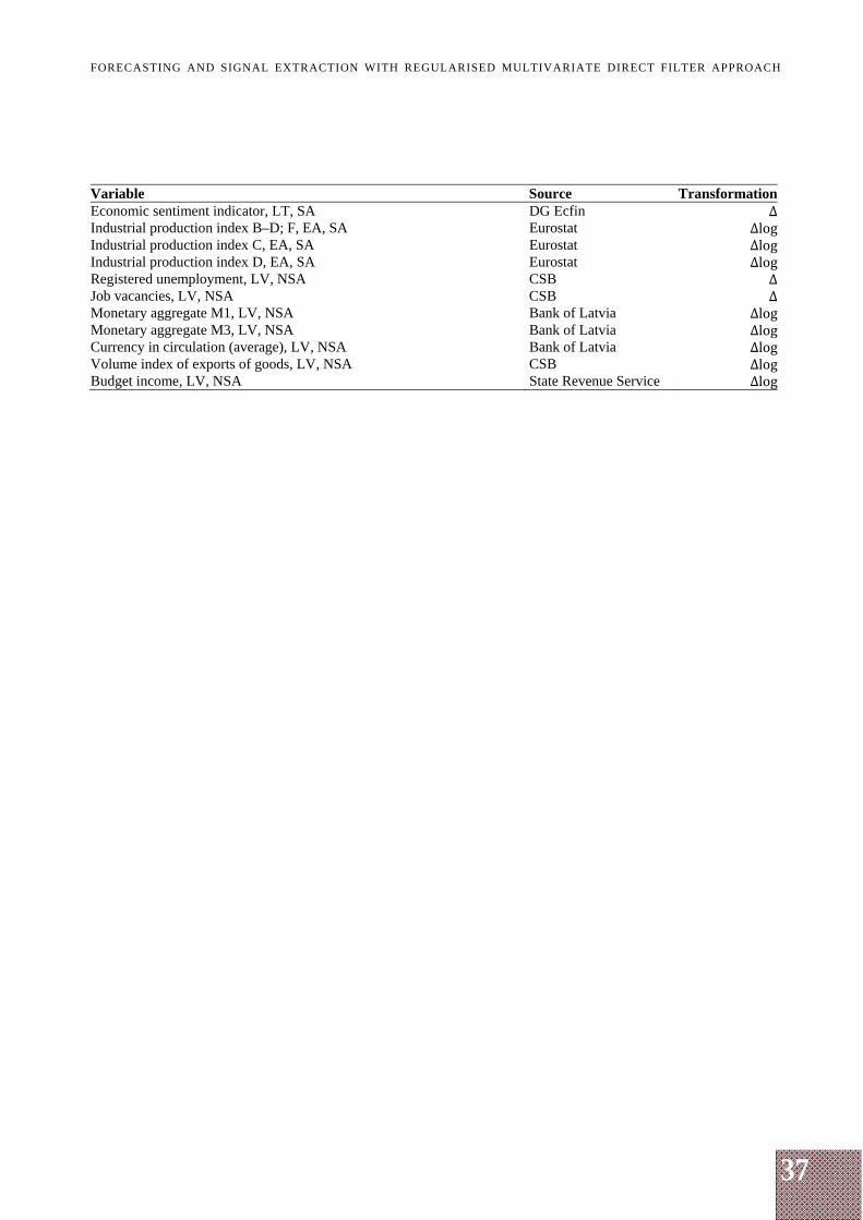
Variable Source Transformation Economic sentiment indicator, LT, SA DG Ecfin ΔIndustrial production index B–D; F, EA, SA Eurostat ΔlogIndustrial production index C, EA, SA Eurostat ΔlogIndustrial production index D, EA, SA Eurostat ΔlogRegistered unemployment, LV, NSA CSB ΔJob vacancies, LV, NSA CSB ΔMonetary aggregate M1, LV, NSA Bank of Latvia ΔlogMonetary aggregate M3, LV, NSA Bank of Latvia ΔlogCurrency in circulation (average), LV, NSA Bank of Latvia ΔlogVolume index of exports of goods, LV, NSA CSB ΔlogBudget income, LV, NSA State Revenue Service Δlog
38
FORECASTING AND SIGNAL EXTRACTION WITH REGULARISED MULTIVARIATE DIRECT FILTER APPROACH
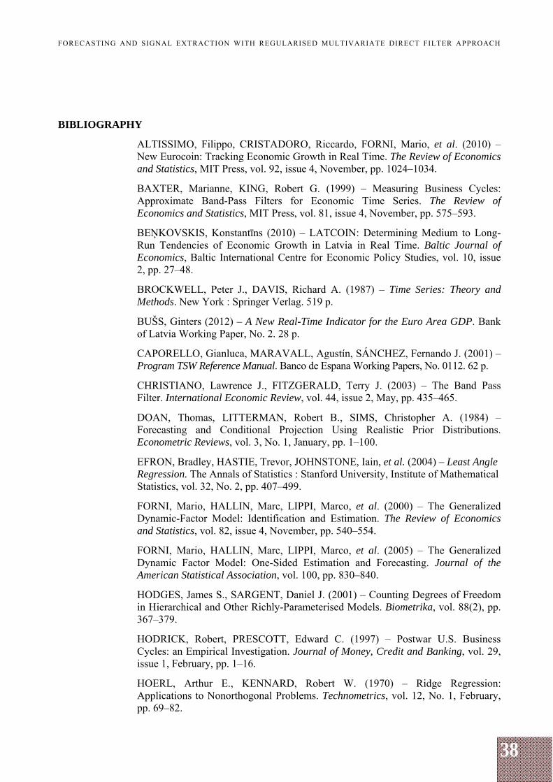
BIBLIOGRAPHY
ALTISSIMO, Filippo, CRISTADORO, Riccardo, FORNI, Mario, et al. (2010) – New Eurocoin: Tracking Economic Growth in Real Time. The Review of Economics and Statistics, MIT Press, vol. 92, issue 4, November, pp. 1024–1034.
BAXTER, Marianne, KING, Robert G. (1999) – Measuring Business Cycles: Approximate Band-Pass Filters for Economic Time Series. The Review of Economics and Statistics, MIT Press, vol. 81, issue 4, November, pp. 575–593.
BEŅKOVSKIS, Konstantīns (2010) – LATCOIN: Determining Medium to Long-Run Tendencies of Economic Growth in Latvia in Real Time. Baltic Journal of Economics, Baltic International Centre for Economic Policy Studies, vol. 10, issue 2, pp. 27–48.
BROCKWELL, Peter J., DAVIS, Richard A. (1987) – Time Series: Theory and Methods. New York : Springer Verlag. 519 p.
BUŠS, Ginters (2012) – A New Real-Time Indicator for the Euro Area GDP. Bank of Latvia Working Paper, No. 2. 28 p.
CAPORELLO, Gianluca, MARAVALL, Agustín, SÁNCHEZ, Fernando J. (2001) – Program TSW Reference Manual. Banco de Espana Working Papers, No. 0112. 62 p.
CHRISTIANO, Lawrence J., FITZGERALD, Terry J. (2003) – The Band Pass Filter. International Economic Review, vol. 44, issue 2, May, pp. 435–465.
DOAN, Thomas, LITTERMAN, Robert B., SIMS, Christopher A. (1984) – Forecasting and Conditional Projection Using Realistic Prior Distributions. Econometric Reviews, vol. 3, No. 1, January, pp. 1–100.
EFRON, Bradley, HASTIE, Trevor, JOHNSTONE, Iain, et al. (2004) – Least Angle Regression. The Annals of Statistics : Stanford University, Institute of Mathematical Statistics, vol. 32, No. 2, pp. 407–499.
FORNI, Mario, HALLIN, Marc, LIPPI, Marco, et al. (2000) – The Generalized Dynamic-Factor Model: Identification and Estimation. The Review of Economics and Statistics, vol. 82, issue 4, November, pp. 540–554.
FORNI, Mario, HALLIN, Marc, LIPPI, Marco, et al. (2005) – The Generalized Dynamic Factor Model: One-Sided Estimation and Forecasting. Journal of the American Statistical Association, vol. 100, pp. 830–840.
HODGES, James S., SARGENT, Daniel J. (2001) – Counting Degrees of Freedom in Hierarchical and Other Richly-Parameterised Models. Biometrika, vol. 88(2), pp. 367–379.
HODRICK, Robert, PRESCOTT, Edward C. (1997) – Postwar U.S. Business Cycles: an Empirical Investigation. Journal of Money, Credit and Banking, vol. 29, issue 1, February, pp. 1–16.
HOERL, Arthur E., KENNARD, Robert W. (1970) – Ridge Regression: Applications to Nonorthogonal Problems. Technometrics, vol. 12, No. 1, February, pp. 69–82.
39
FORECASTING AND SIGNAL EXTRACTION WITH REGULARISED MULTIVARIATE DIRECT FILTER APPROACH
KING, Robert G., REBELO, Sergio T. (1993) – Low Frequency Filtering and Real Business Cycles. Journal of Economic Dynamics and Control, vol. 17, issue 1–2, pp. 207–231.
MARAVALL, Agustin, RIO, Ana del (2001) – Time Aggregation and the Hodrick-Prescott Filter. Banco de Espana Working Papers, No. 0108, March. 44 p.
MOODY, John E. (1992) – The Effective Number of Parameters: an Analysis of Generalization and Regularization in Nonlinear Learning Systems. In: Advances in Neural Information Processing Systems 4. Edited by J. E. Moody, S. J. Hanson and R. P. Lippmann. San Mateo : Morgan Kaufmann, pp. 847–854.
STOCK, James H., WATSON, Mark W. (2002) – Macroeconomic Forecasting Using Diffusion Indexes. Journal of Business & Economic Statistics, vol. 20, No. 2, pp. 147–162.
TIBSHIRANI, Robert (1996) – Regression Shrinkage and Selection via the Lasso. Journal of the Royal Statistical Society, Series B (Methodological), vol. 58, No. 1, pp. 267–288.
TIKHONOV, Andrey, ARSENIN, Vasiliy (1977) – Solutions of Ill-Posed Problems. Washington : V. H. Winston & Sons. 258 p.
VALLE E AZEVEDO, João (2011) – A Multivariate Band-Pass Filter for Economic Time Series. Journal of the Royal Statistical Society Series C, vol. 60, issue 1, January, pp. 1–30.
WILDI, Marc (2008) – Real-Time Signal-Extraction: Beyond Maximum Likelihood Principles. October [cited 30 November 2012]. Available: http://blog.zhaw.ch/idp/sefblog/uploads/Wildi_Real_Time_SE_0810010.pdf.
WILDI, Marc (2011) – I-DFA and I-MDFA: Companion Paper to R-code Published on SEFBlog. IDP-Working Paper, March [cited 30 November 2012]. Available: http://blog.zhaw.ch/idp/sefblog/uploads/working_paper1.pdf.
WILDI, Marc (2012) – Elements of Forecasting and Signal Extraction. IDP-Working Paper, August [cited 30 November 2012]. Available: http://blog.zhaw.ch/idp/sefblog/uploads/elements_3007.pdf.