Forecasting annual natural gas consumption via the

RESEARCH ARTICLE

Forecasting annual natural gas consumption via the applicationof a novel hybrid model

Feng Gao1,2& Xueyan Shao1,2

Received: 27 October 2020 /Accepted: 28 December 2020# The Author(s), under exclusive licence to Springer-Verlag GmbH, DE part of Springer Nature 2021

AbstractAccurate prediction of natural gas consumption (NGC) can offer effective information for energy planning and policy-making. Inthis study, a novel hybrid forecasting model based on support vector machine (SVM) and improved artificial fish swarmalgorithm (IAFSA) is proposed to predict annual NGC. An adaptive learning strategy based on sigmoid function is introducedto improve the performance of traditional artificial fish swarm algorithm (AFSA), which provides a dynamic adjustment forparameter moving step step and visual scope visual. IAFSA is used to obtain the optimal parameters of SVM. In addition, theannual NGC data of China is selected as an example to evaluate the prediction performance of the proposed model. Experimentalresults reveal that the proposed model in this study outperforms the benchmark models such as artificial neural network (ANN)and partial least squares regression (PLS). The mean absolute percentage error (MAPE), root mean squared error (RMSE), andmean absolute error (MAE) values are as low as 0.512, 1.4958, and 1.0940. Finally, the proposed model is employed to predictNGC in China from 2020 to 2025.

Keywords Support vectormachine . Improved artificial fish swarm algorithm . Natural gas consumption forecasting

Introduction

Global warming is a serious problem for countries all over theworld, threatening the survival and development of humanbeings. Overuse of traditional fossil energy is the main causeof global warming. After the Copenhagen Conference, mostcountries began to explore clean and low-carbon energy tran-sition, striving to reduce carbon emissions (Lu et al. 2020).Due to its cleanliness and high efficiency, natural gas becomesthe best transitional energy in the process of clean and low-carbon energy transition. According to BP Energy Outlook2020, it is projected that the global demand for natural gaswill grow robustly over the next 15 years (BP 2020). As thedemand rises, it is necessary for governments to formulate areasonable natural gas plan in advance to ensure sufficientnatural gas supplies and transmission infrastructures.

Improper estimation of natural gas consumption (NGC) maylead to the imbalance of natural gas supply and demand, caus-ing social economic losses (Shaikh and Ji 2016).Consequently, accurate prediction of NGC has great signifi-cance to the formulation of an energy policy and plan.

However, forecasting NGC is a challenging task. NGC isaffected by various external factors, such as population andeconomic development, and the relationship between influ-ence factors and NGC is nonlinear (Kavaklioglu 2011).Besides, the natural gas consumption time series (in particularyearly) data have the characteristics of nonlinearity, volatility,and small samples (Lu et al. 2020). In this case, it is verydifficult to establish an accurate prediction model. Therefore,how to improve the prediction accuracy of NGC is a veryimportant issue in the field of energy prediction.

Up to now, a large number of scholars have conductedstudies on NGC prediction methods. Grey forecastingmodels and regression models are the most popularmethods, widely used in NGC forecasting. For example,Shaikh et al. (2017) and Ding (2018) constructed China’syearly NGC forecasting model by utilizing grey models.Ozdemir et al. (2016) and Melikoglu (2013) employed linearregression to forecast natural gas demand in Turkey. With thedevelopment of artificial intelligence technology, machine

Responsible Editor: Marcus Schulz

* Xueyan [email protected]

1 Institutes of Science and Development, Chinese Academy ofSciences, Beijing 100190, China

2 University of Chinese Academy of Sciences, Beijing 100049, China

https://doi.org/10.1007/s11356-020-12275-w

/ Published online: 7 January 2021

Environmental Science and Pollution Research (2021) 28:21411–21424

http://crossmark.crossref.org/dialog/?doi=10.1007/s11356-020-12275-w&domain=pdf

mailto:[email protected]

learning forecasting models have been introduced to predictNGC. Szoplik (2015) used artificial neural networks (ANN) toforecast daily NGC in Szczecin (Poland). Wei et al. (2019)proposed a hybrid model combining improved singular spec-trum analysis and long short-term memory to forecast dailyNGC.

Despite some progress made in NGC prediction modelstudies, there are still some research gaps worthy of furtherexploration. In the current researches, the annual NGC fore-casting is mainly based on grey prediction models and multi-ple regression models. To the best of our knowledge, there arefew studies which apply machine learning models for long-term (annual) NGC forecasting. In fact, some machine learn-ing models, such as support vector machine (SVM), haveexcellent fitting capabilities for nonlinear small sample data.For instance, Kavaklioglu (2011) applied SVM to predictTurkey’s electricity consumption using data from 1975 to2006. The first 26 data are used for training and theremaining data are used for testing. Compared with randomwalk, SVMhas a lower error.Ma et al. (2019) employed SVMto forecast building energy consumption in southern Chinawith the test sample from 2000 to 2014. Forecasting resultsshow that SVM can estimate building energy consumptionwith accuracy with MSE less than 0.001. However, the learn-ing performance and generalization ability of SVM largelydepends on the model parameters (Cherkassky and Ma2004). To tackle this problem, some intelligent optimizationalgorithms are used to optimize parameters of SVM, such asgenetic algorithm (GA) (Huang and Wang 2006) and particleswarm optimization algorithm (PSO) (Jiang et al. 2011; Menget al. 2014). But these traditional intelligent optimization al-gorithms are prone to premature maturity and fall into localoptimum (Chen et al. 2008), which may reduce the predictionaccuracy.

In this paper, a novel hybrid forecasting model is proposedto predict annual NGC. The proposed model combines sup-port vector machine (SVM) and improved artificial fishswarm algorithm (IAFSA), making full use of the ability toprocess small samples of SVM and the global optimizationcapabilities of IAFSA. IAFSA is used to optimize the param-eters of SVM. The purpose of this study is to improve theprediction accuracy of NGC and provide more effective infor-mation for energy planning and policy-making.

The main contributions of this study are concluded as fol-lows: First, an adaptive learning strategy based on sigmoidfunction is introduced to improve the traditional artificial fishswarm algorithm (AFSA), dealing with imbalance betweenlocal search and global search caused by fixed initial values.Three standard test functions are used to verify the strategy.Simulating results reveal that IAFSA has stronger search abil-ity. Second, a novel hybrid model based on SVM and IAFSAis proposed to predict annual NGC. China’s NGC data isapplied to validate forecasting performance of the proposed

model. Experimental results show that the proposed modelperforms much better than benchmark models.

The rest of this study is organized as follows: “Literaturereview” presents the previous literature. “Methodology” intro-duces the foundation of support vector machine (SVM) andartificial fish swarm algorithm (AFSA), and proposes the im-proved artificial fish swarm algorithm (IAFSA). “Data de-scription” describes the data in detail. “Experimental resultsand discussion” presents the experimental results of IAFSA-SVM and compares with benchmark models to demonstratethe forecasting performance of IAFSA-SVM. “Conclusionsand future work” draws some conclusions and proposes futurework.

Literature review

Influence factors of NGC

Analyzing and finding out the influence factors of natural gasconsumption (NGC) is the key to forecasting NGC. In recentyears, a large amount of literature has conducted research onthe influencing factors of NGC, as summarized in Table 1. Forexample, Wang and Li (2020) applied grey relationship anal-ysis to study the influence factors of natural gas demand inChina’s eastern, central, and western regions. Results showedthat GDP, energy consumption structure, urbanization rate,industrial structure, and population density are the main fac-tors affecting China’s natural gas demand. Similarly,Melikoglu (2013) selected GDP and population as influencefactors to estimate Turkey’s NGC. Besides GDP andpopulation, Wadud et al. (2011) considered natural gas pricesas the main external driver that affect Bangladesh’s NGC.According to his study, the relationship between NGC andGDP is positive while the relationship between NGC andnatural gas price is negative. Khan (2015) studied the relation-ship between income, natural gas price and price of substi-tutes, and Pakistan’s NGC. The research results reveal thatincome is positively correlated with NGC in the short andlong run, and natural gas price is negatively correlated withNGC. The price of substitutes has no significant impact onNGC in the short run, but has a weak positive correlation inthe long run. Furthermore, through qualitative analysis,Hongxun and Hui (2019) found out the factors affectingChina’s NGC including GDP, total population, urbanizationrate, natural gas pipeline construction, energy consumptionstructure, carbon emissions, etc.

The above-mentioned literature analyzed the factors affect-ing NGC from various aspects, and verified the relationshipbetween various influence factors and NGC. Due to differentconditions and development stages in various countries, theinfluencing factors of NGC are different. To sum up, gross

21412 Environ Sci Pollut Res (2021) 28:21411–21424

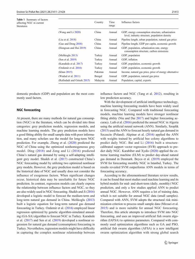
domestic products (GDP) and population are the most com-monly used factors.

NGC forecasting

At present, there are many methods for natural gas consump-tion (NGC) in the literature, which can be divided into threecategories: grey prediction models, regression models, andmachine learning models. The grey prediction models havea good fitting ability for small sample data with poor informa-tion, and many scholars use the model for long-term NGCprediction. For example, Zheng et al. (2020) predicted theNGC of China using the optimized nonhomogeneous greymodel. Ding (2018) and Zeng and Li (2016) predictedChina’s natural gas demand by using a self-adapting intelli-gent grey model. Shaikh et al. (2017) constructed China’sNGC forecasting model by utilizing two optimized nonlineargrey models. However, the grey prediction model is based onthe historical data of NGC and usually does not consider theinfluence of exogenous factors. When significant changesoccur, historical data may be unreliable for future NGCprediction. In contrast, regression models can clearly expressthe relationship between influence factors and NGC, so theyare also widely used in NGC forecasting. Shaikh and Ji (2016)developed a logistic model to forecast the medium-term andlong-term natural gas demand in China. Melikoglu (2013)built a logistic equation for long-term natural gas demandforecasting in Turkey. Ozdemir et al. (2016) employed linearregression optimized by genetic algorithm-simulated anneal-ing (GA-SA) algorithm to forecast NGC in Turkey. Karadedeet al. (2017) and Sen et al. (2019) developed a nonlinear re-gression for natural gas demand (consumption) forecasting inTurkey. Nevertheless, regressionmodels might have difficultyin capturing the complex nonlinear relationship between

influence factors and NGC (Tang et al. 2012), resulting inlow prediction accuracy.

With the development of artificial intelligence technology,machine learning forecasting models have been widely usedin forecasting NGC. Compared with traditional forecastingmodels, machine learning models have stronger nonlinearfitting ability (Niu and Dai 2017) and higher forecasting ac-curacy. Laib et al. (2016) predicted the annual NGC in Algeriausing the artificial neural network (ANN). Similarly, Szoplik(2015) used the ANN to forecast hourly natural gas demand inSzczecin (Poland). Akpinar et al. (2016) applied the ANNwith weights trained by artificial bee colony algorithms topredict daily NGC. Bai and Li (2016) built a structure-calibrated support vector regression (SVR) approach to pre-dict daily NGC. Karabiber and Xydis (2020) applied the ex-treme learning machine (ELM) to predict day-ahead naturalgas demand in Denmark. Beyca et al. (2019) employed theSVM for forecasting monthly NGC in Istanbul, Turkey. Theresults revealed SVM outperforms ANN models in terms offorecasting accuracy.

According to the aforementioned literature review results,it can be found that most studies used machine learning and itshybrid models for mid- and short-term (daily, monthly) NGCprediction, and only a few studies applied ANN to predictannual NGC. However, ANN requires a lot of training data,which is not suitable for annual NGC data (small samples).Compared with ANN, SVM adopts the structural risk mini-mization criterion to process small sample data (Mirzaei et al.2015) and is more suitable for annual NGC forecasting.Therefore, this article attempts to introduce SVM into NGCforecasting, and uses an improved artificial fish swarm algo-rithm (IAFSA) to optimize parameters. Compared with com-monly used optimization algorithms such as GA and PSO,artificial fish swarm algorithm (AFSA) is a new intelligentswarm optimization algorithm with strong global search

Table 1 Summary of factorsaffecting NGC in currentliteratures

Country Timerange

Influence factors

(Wang and Li 2020) China Annual GDP, energy consumption structure, urbanizationlevel, industry structure, population density

(Liu et al. 2018) China Annual Pipeline length, urban population, natural gas price

(Gao and Dong 2018) China Annual Pipeline length, GDP per capita, economic growth

(Hongxun and Hui 2019) China Annual GDP, population, urbanization rate, energyconsumption structure, carbon emissions

(Melikoglu 2013) Turkey Annual GDP, population

(Sen et al. 2019) Turkey Annual GDP, inflation

(Karadede et al. 2017) Turkey Annual GDP, population, economic growth

(Ozdemir et al. 2016) Turkey Annual GDP, population, economic growth

(Khan 2015) Pakistan Annual Income, natural gas price, price of energy alternative

(Wadud et al. 2011) Bengal Annual GDP, population, natural gas price

(Rafindadi and Ozturk 2015) Malaysia Annual Population, capital, exports

21413Environ Sci Pollut Res (2021) 28:21411–21424

ability and good robustness, and is not sensitive to initial pa-rameters (Chen et al. 2008). In order to further improve theoptimization accuracy, an adaptive leaning strategy based onsigmoid function is introduced to improve AFSA.

Methodology

SVM

Support vector machine (SVM) is a machine learning algo-rithm based on the principles of structural risk minimization(Xue and Yang 2016). It has good generalization ability forsmall sample, nonlinear and high-dimensional feature data(Mirzaei et al. 2015). Not only does SVM perform well inclassification prediction, but it can also be used in regressionestimation problems (Vapnik 1998). The support vector re-gression model has good fitting and predictive ability underthe condition of small sample and nonlinearity.

Given the training set is (Xi, yi), i = 1, 2,…, n, X ∈ Rm, y ∈R, where Xi is the input vector and yi is the output vector. Theregression function can be expressed as

f xð Þ ¼ ω∙Xð Þ þ b;ω∈Rm; b∈R ð1Þwhere ω is the weighted vector, b is the bias, and Rm and Rrepresent m-dimensional vector space and one-dimensionalvector space respectively.

We can estimate ω and b through structural risk minimiza-tion; the expression is as follows:

minR fð Þ ¼ 1

2ωk k2 þ C

2∑n

i¼1L yi; f X ið Þð Þ ð2Þ

where L is loss function and C is penalty factor.

Introducing the relaxation variables ξi and ξ*i , formula (2) can

be transformed into a convex quadratic optimization problem:

min1

2ωk k2 þ C∑n

i¼1 ξi þ ξ*i� � ð3Þ

s:t:yi−ω∙X i−b≤εþ ξiω∙X i þ b−yi≤εþ ξ*i

ξi; ξ*i ≥0; i ¼ 1; 2;…; n

8<: ð4Þ

The Lagrange function is introduced and converted intodual form:

max −1

2∑n

i; j¼1αi−α*

i

� �α j−α*

j

� �X i∙X j� �

−ε∑ni¼1 αi þ α*

i

� �þ ∑ni¼1yi αi−α*

i

� �ð5Þ

s:t: ∑ni¼1 αi−α*

i

� � ¼ 0;αi;α*i ∈ 0;C½ � ð6Þ

The regression function is as follows:

f Xð Þ ¼ ∑ni¼1 αi−α*

i

� �X i;Xð Þ þ b ð7Þ

Introducing kernel function, formula (7) can be expressedas

f Xð Þ ¼ ∑ni¼1 αi−α*

i

� �K X i;Xð Þ þ b ð8Þ

where K(Xi, X) is the kernel function.The selection of kernel functions is a key issue of the SVM

method, and different kernel functions can lead to differentgeneralization and learning ability of prediction models (Luet al. 2019). There are three kinds of kernel functions whichare commonly used: polynomial function (Eq. (9)), radial ba-sis function (Eq. (10)), and linear function (Eq. (11)).

K X i;Xð Þ ¼ X i∙X þ 1ð Þd ð9Þ

K X i;Xð Þ ¼ e−γ

�X i−X

�� 2

ð10ÞK X i;Xð Þ ¼ X i∙X ð11Þ

Among them, radial basis kernel function, also calledGaussian kernel function, has excellent adaptability and rec-ognition accuracy for small sample and nonlinear problems.Therefore, this study uses the radial basis kernel function. ForSVMwith radial basis kernel function, the parameters includepenalty factor C and kernel parameter γ.

IAFSA

Artificial fish swarm algorithm

Artificial fish swarm algorithm (AFSA) is a new bionic opti-mization algorithm, proposed by Xiaolei Li in 2002 (Li et al.2002). The core idea is to solve the optimization problem bysimulating the behaviors of natural fish searching for food inwater. In AFSA, the position of the artificial fish represents afeasible solution to the optimization problem. The optimiza-tion goal of AFSA is to find the position with the highest foodconcentration among the fish swarm, which also representsthe optimal solution of the optimization problem (Zhenget al. 2019).

Suppose the search space isD-dimensional and there are Nartificial fishes in total. The current position of fish i isXi = (x1, x2,…, xD)(i = 1, 2, ..,N), and the fitness function alsocalled objective function, which means the food concentrationof current position, is Yi = f(Xi). The distance between fish iand fish j can be calculated by dij = ‖Xi − Xj‖. There are someother important parameters, including the moving step step,visual scope visual, crowded degree δ, and so on. In AFSA, anartificial fish performs preying behavior, swarming behavior,following behavior, and random behavior to search for the


position with higher food concentration and record the opti-mal position on the bulletin board.

(1) Preying behavior

Preying behavior is a behavior in which an artificial fishswims to the positionwith higher food concentration. Supposethe current position of the artificial fish i is Xi, we randomlyselect a new position Xjwithin its visual scope (dij < visual); Yiand Yj are the corresponding fitness values. If, in a minimumproblem, Yj < Yi, Xi moves a step toward Xj. Otherwise, con-tinue to search within its visual scope and judge whether thenew position satisfies the forward condition. If it still cannotbe satisfied when the number of tries is greater than the max-imum number of tries, perform random behavior. Preying be-havior can be expressed as follows:

X next ¼ X i þ randðÞ∙step∙ X j−X i

X j−X i�� ð12Þ

where rand() represents a random number between 0 and 1,and Xnext is the next position of artificial fish i.

(2) Random behavior

Random behavior is a behavior in which the artificial fishswims randomly within its visual scope, which is a defaultbehavior of preying behavior. Random behavior can beexpressed as follows:

X j ¼ X i þ randðÞ∙step ð13Þ

(3) Swarming behavior

In order to avoid danger, a fish swarm will spontaneouslygather in groups. Within the visual scope of Xi(dij < visual), Xcis the central position of the fish swarm, and nf is the number

of companions. If Yc n f < δY i, it means that Xc is not toocrowded with higher food concentration; Xi moves a step to-ward Xc. Otherwise, perform preying behavior. The swarmingbehavior can be expressed as follows:

X next ¼ X i þ randðÞ∙step∙ X c−X i

X c−X ik k ð14Þ

(4) Following behavior

When one or more artificial fish find food, fish nearby willfollow. Within a visual scope of Xi(dij < visual), Xmax is the

position with the highest food concentration. If Ymax nf < δY i,

it means Xmax is not too crowded with higher food concentra-tion; Xi moves a step toward Xmax. Otherwise, conduct preyingbehavior. The following behavior can be expressed as follows:

X next ¼ X i þ randðÞ∙step∙ Xmax−X i

Xmax−X ik k ð15Þ

(5) Bulletin board

The bulletin board is a place to record the status of the bestindividual. After an iteration, each artificial fish will compareits current fitness value with the fitness value recorded on thebulletin board. If it is less than the fitness value on the bulletinboard, update the bulletin board with the current position andfitness value; otherwise, the state of the bulletin board willremain unchanged. When the iteration of the whole algorithmis finished, the output value of the bulletin board is the optimalvalue (Bai et al. 2017).

Improved AFSA

In artificial fish swarm algorithm (AFSA), moving step step(hereafter step) and visual scope visual (hereafter visual) aretwo important parameters, influencing the optimization per-formance of the algorithm. But they are fixed values, remain-ing unchanged during the iteration process, which makes itdifficult to give suitable initial values. If the values of stepand visual are too large, the artificial fish can move to theglobal optimal value rapidly in the early stage, but there willbe an oscillation phenomenon in the later stage and it is diffi-cult to reach the optimal value accurately. If the values are toosmall, the artificial fish can reach the optimal value accuratelybut converge slowly, easy to fall into local optimum.

In order to tackle the problem aforementioned, an adaptivelearning strategy of step and visual is proposed in this study.Inspired by the characteristics of sigmoid function, a dynam-ical weight is introduced to adjust step and visual of artificialfish to balance local search and global search. In the iterationprocess of IAFSA, the larger step and visual make the algo-rithm quickly converge and jump out of the local optimum inthe early stage. The smaller step and visual can make thealgorithm accurately approach the global optimum and im-prove the accuracy in the later stage. The improved stepand visual are expressed as follows:

μ ¼ 1−1

1þ e−iter

itermax−α

β ; 0≤α;β≤1ð16Þ

stepiter ¼ stepiter−1∙μ ð17Þvisualiter ¼ visualiter−1∙μ ð18Þ


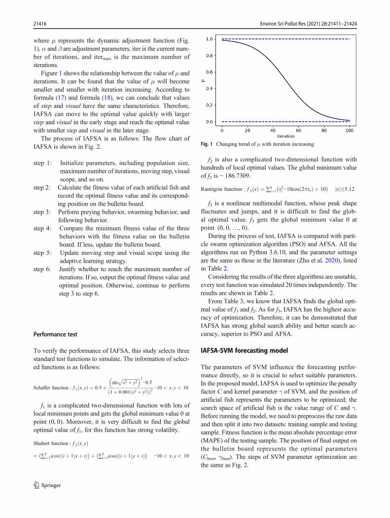
where μ represents the dynamic adjustment function (Fig.1), α and β are adjustment parameters, iter is the current num-ber of iterations, and itermax is the maximum number ofiterations.

Figure 1 shows the relationship between the value of μ anditerations. It can be found that the value of μ will becomesmaller and smaller with iteration increasing. According toformula (17) and formula (18), we can conclude that valuesof step and visual have the same characteristics. Therefore,IAFSA can move to the optimal value quickly with largerstep and visual in the early stage and reach the optimal valuewith smaller step and visual in the later stage.

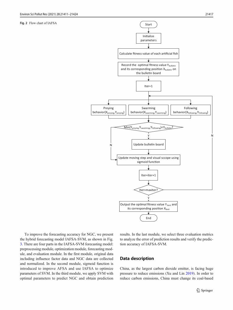
The process of IAFSA is as follows: The flow chart ofIAFSA is shown in Fig. 2.

step 1: Initialize parameters, including population size,maximum number of iterations, moving step, visualscope, and so on.

step 2: Calculate the fitness value of each artificial fish andrecord the optimal fitness value and its correspond-ing position on the bulletin board.

step 3: Perform preying behavior, swarming behavior, andfollowing behavior.

step 4: Compare the minimum fitness value of the threebehaviors with the fitness value on the bulletinboard. If less, update the bulletin board.

step 5: Update moving step and visual scope using theadaptive learning strategy.

step 6: Justify whether to reach the maximum number ofiterations. If so, output the optimal fitness value andoptimal position. Otherwise, continue to performstep 3 to step 6.

Performance test

To verify the performance of IAFSA, this study selects threestandard test functions to simulate. The information of select-ed functions is as follows:

Schaffer function : f 1 x; yð Þ ¼ 0:5þsin

ffiffiffiffiffiffiffiffiffiffiffiffiffiffix2 þ y2

p� �2−0:5

1þ 0:001 x2 þ y2ð Þð Þ2 −10 < x; y < 10

f1 is a complicated two-dimensional function with lots oflocal minimum points and gets the global minimum value 0 atpoint (0, 0). Moreover, it is very difficult to find the globaloptimal value of f1, for this function has strong volatility.

Shubert function : f 2 x; yð Þ

¼ ∑5i¼1icos iþ 1ð Þxþ ið Þ� �þ ∑5

i¼1icos iþ 1ð Þyþ ið Þ� �−10 < x; y < 10

f2 is also a complicated two-dimensional function withhundreds of local optimal values. The global minimum valueof f2 is − 186.7309.

Rastrigrin function : f 3 xð Þ ¼ ∑ni¼1 x2i −10cos 2πxið Þ þ 10

� �xj j≤5:12

f3 is a nonlinear multimodal function, whose peak shapefluctuates and jumps, and it is difficult to find the glob-al optimal value. f3 gets the global minimum value 0 atpoint (0, 0,…, 0).

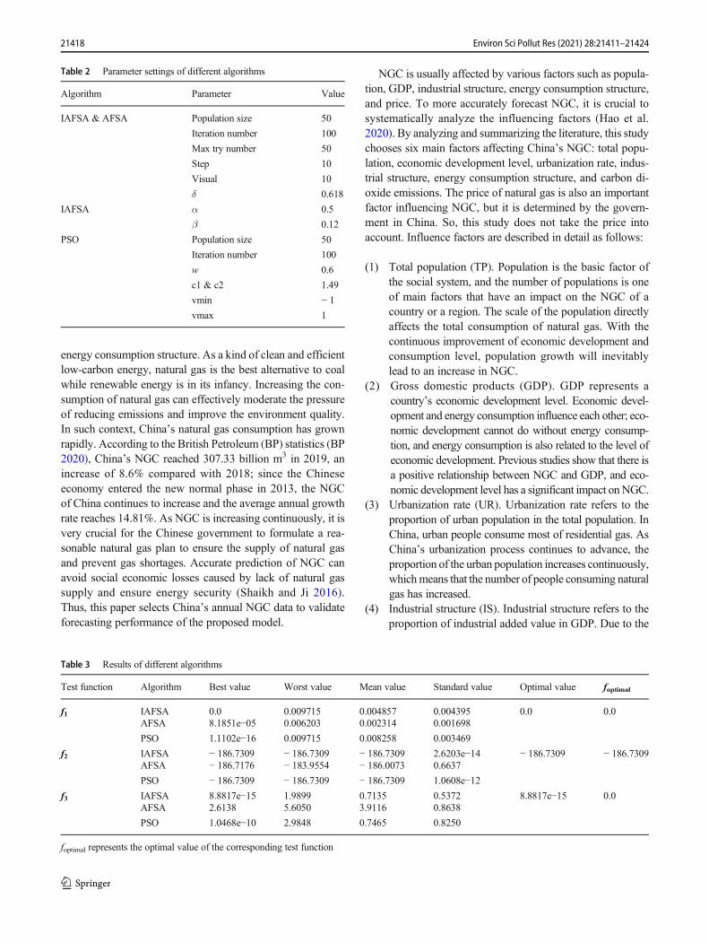
During the process of test, IAFSA is compared with parti-cle swarm optimization algorithm (PSO) and AFSA. All thealgorithms run on Python 3.6.10, and the parameter settingsare the same as those in the literature (Zhu et al. 2020), listedin Table 2.

Considering the results of the three algorithms are unstable,every test function was simulated 20 times independently. Theresults are shown in Table 2.

From Table 3, we know that IAFSA finds the global opti-mal value of f1 and f2. As for f3, IAFSA has the highest accu-racy of optimization. Therefore, it can be demonstrated thatIAFSA has strong global search ability and better search ac-curacy, superior to PSO and AFSA.

IAFSA-SVM forecasting model

The parameters of SVM influence the forecasting perfor-mance directly, so it is crucial to select suitable parameters.In the proposed model, IAFSA is used to optimize the penaltyfactor C and kernel parameter γ of SVM, and the position ofartificial fish represents the parameters to be optimized; thesearch space of artificial fish is the value range of C and γ.Before running the model, we need to preprocess the raw dataand then split it into two datasets: training sample and testingsample. Fitness function is the mean absolute percentage error(MAPE) of the testing sample. The position of final output onthe bulletin board represents the optimal parameters(Cbest, γbest). The steps of SVM parameter optimization arethe same as Fig. 2.

Fig. 1 Changing trend of μ with iteration increasing


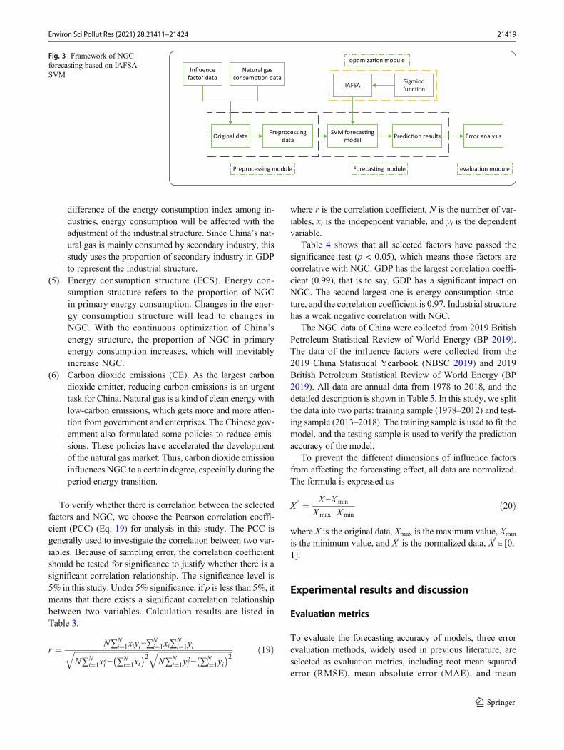
To improve the forecasting accuracy for NGC, we presentthe hybrid forecasting model IAFSA-SVM, as shown in Fig.3. There are four parts in the IAFSA-SVM forecasting model:preprocessingmodule, optimizationmodule, forecastingmod-ule, and evaluation module. In the first module, original dataincluding influence factor data and NGC data are collectedand normalized. In the second module, sigmoid function isintroduced to improve AFSA and use IAFSA to optimizeparameters of SVM. In the third module, we apply SVM withoptimal parameters to predict NGC and obtain prediction

results. In the last module, we select three evaluation metricsto analyze the error of prediction results and verify the predic-tion accuracy of IAFSA-SVM.

Data description

China, as the largest carbon dioxide emitter, is facing hugepressure to reduce emissions (Xu and Lin 2019). In order toreduce carbon emissions, China must change its coal-based

Start

Ini�alize parameters

Calculate fitness value of each ar�ficial fish

Record the op�mal fitness value Ybulle�nand its corresponding posi�on Xbulle�n on

the bulle�n board

Preying behavior(Xpreying,Ypreying)

Swarming behavior(Xswarming,Yswarming)

Following behavior(Xfollowing,Yfollowing)

Min(Ypreying,Yswarming,Yfollowing)<Ybulle�n?

Update bulle�n board

Iter>maxiter?

Output the op�mal fitness value Y best and its corresponding posi�on Xbest

Y

End

Y

Update moving step and visual sccope using sigmoid func�on

N

Iter=1

Iter=iter+1

N

Fig. 2 Flow chart of IAFSA


energy consumption structure. As a kind of clean and efficientlow-carbon energy, natural gas is the best alternative to coalwhile renewable energy is in its infancy. Increasing the con-sumption of natural gas can effectively moderate the pressureof reducing emissions and improve the environment quality.In such context, China’s natural gas consumption has grownrapidly. According to the British Petroleum (BP) statistics (BP2020), China’s NGC reached 307.33 billion m3 in 2019, anincrease of 8.6% compared with 2018; since the Chineseeconomy entered the new normal phase in 2013, the NGCof China continues to increase and the average annual growthrate reaches 14.81%. As NGC is increasing continuously, it isvery crucial for the Chinese government to formulate a rea-sonable natural gas plan to ensure the supply of natural gasand prevent gas shortages. Accurate prediction of NGC canavoid social economic losses caused by lack of natural gassupply and ensure energy security (Shaikh and Ji 2016).Thus, this paper selects China’s annual NGC data to validateforecasting performance of the proposed model.

NGC is usually affected by various factors such as popula-tion, GDP, industrial structure, energy consumption structure,and price. To more accurately forecast NGC, it is crucial tosystematically analyze the influencing factors (Hao et al.2020). By analyzing and summarizing the literature, this studychooses six main factors affecting China’s NGC: total popu-lation, economic development level, urbanization rate, indus-trial structure, energy consumption structure, and carbon di-oxide emissions. The price of natural gas is also an importantfactor influencing NGC, but it is determined by the govern-ment in China. So, this study does not take the price intoaccount. Influence factors are described in detail as follows:

(1) Total population (TP). Population is the basic factor ofthe social system, and the number of populations is oneof main factors that have an impact on the NGC of acountry or a region. The scale of the population directlyaffects the total consumption of natural gas. With thecontinuous improvement of economic development andconsumption level, population growth will inevitablylead to an increase in NGC.

(2) Gross domestic products (GDP). GDP represents acountry’s economic development level. Economic devel-opment and energy consumption influence each other; eco-nomic development cannot do without energy consump-tion, and energy consumption is also related to the level ofeconomic development. Previous studies show that there isa positive relationship between NGC and GDP, and eco-nomic development level has a significant impact onNGC.

(3) Urbanization rate (UR). Urbanization rate refers to theproportion of urban population in the total population. InChina, urban people consume most of residential gas. AsChina’s urbanization process continues to advance, theproportion of the urban population increases continuously,whichmeans that the number of people consuming naturalgas has increased.

(4) Industrial structure (IS). Industrial structure refers to theproportion of industrial added value in GDP. Due to the

Table 2 Parameter settings of different algorithms

Algorithm Parameter Value

IAFSA & AFSA Population size 50

Iteration number 100

Max try number 50

Step 10

Visual 10

δ 0.618

IAFSA α 0.5

β 0.12

PSO Population size 50

Iteration number 100

w 0.6

c1 & c2 1.49

vmin − 1

vmax 1

Table 3 Results of different algorithms

Test function Algorithm Best value Worst value Mean value Standard value Optimal value foptimal

f1 IAFSA 0.0 0.009715 0.004857 0.004395 0.0 0.0AFSA 8.1851e−05 0.006203 0.002314 0.001698

PSO 1.1102e−16 0.009715 0.008258 0.003469

f2 IAFSA − 186.7309 − 186.7309 − 186.7309 2.6203e−14 − 186.7309 − 186.7309AFSA − 186.7176 − 183.9554 − 186.0073 0.6637

PSO − 186.7309 − 186.7309 − 186.7309 1.0608e−12f3 IAFSA 8.8817e−15 1.9899 0.7135 0.5372 8.8817e−15 0.0

AFSA 2.6138 5.6050 3.9116 0.8638

PSO 1.0468e−10 2.9848 0.7465 0.8250

foptimal represents the optimal value of the corresponding test function


difference of the energy consumption index among in-dustries, energy consumption will be affected with theadjustment of the industrial structure. Since China’s nat-ural gas is mainly consumed by secondary industry, thisstudy uses the proportion of secondary industry in GDPto represent the industrial structure.

(5) Energy consumption structure (ECS). Energy con-sumption structure refers to the proportion of NGCin primary energy consumption. Changes in the ener-gy consumption structure will lead to changes inNGC. With the continuous optimization of China’senergy structure, the proportion of NGC in primaryenergy consumption increases, which will inevitablyincrease NGC.

(6) Carbon dioxide emissions (CE). As the largest carbondioxide emitter, reducing carbon emissions is an urgenttask for China. Natural gas is a kind of clean energy withlow-carbon emissions, which gets more and more atten-tion from government and enterprises. The Chinese gov-ernment also formulated some policies to reduce emis-sions. These policies have accelerated the developmentof the natural gas market. Thus, carbon dioxide emissioninfluences NGC to a certain degree, especially during theperiod energy transition.

To verify whether there is correlation between the selectedfactors and NGC, we choose the Pearson correlation coeffi-cient (PCC) (Eq. 19) for analysis in this study. The PCC isgenerally used to investigate the correlation between two var-iables. Because of sampling error, the correlation coefficientshould be tested for significance to justify whether there is asignificant correlation relationship. The significance level is5% in this study. Under 5% significance, if p is less than 5%, itmeans that there exists a significant correlation relationshipbetween two variables. Calculation results are listed inTable 3.

r ¼ N∑Ni¼1xiyi−∑

Ni¼1xi∑

Ni¼1yiffiffiffiffiffiffiffiffiffiffiffiffiffiffiffiffiffiffiffiffiffiffiffiffiffiffiffiffiffiffiffiffiffiffiffiffiffiffi

N∑Ni¼1x

2i − ∑N

i¼1xi� �2q ffiffiffiffiffiffiffiffiffiffiffiffiffiffiffiffiffiffiffiffiffiffiffiffiffiffiffiffiffiffiffiffiffiffiffiffiffiffi

N∑Ni¼1y

2i − ∑N

i¼1yi� �2q ð19Þ

where r is the correlation coefficient, N is the number of var-iables, xi is the independent variable, and yi is the dependentvariable.

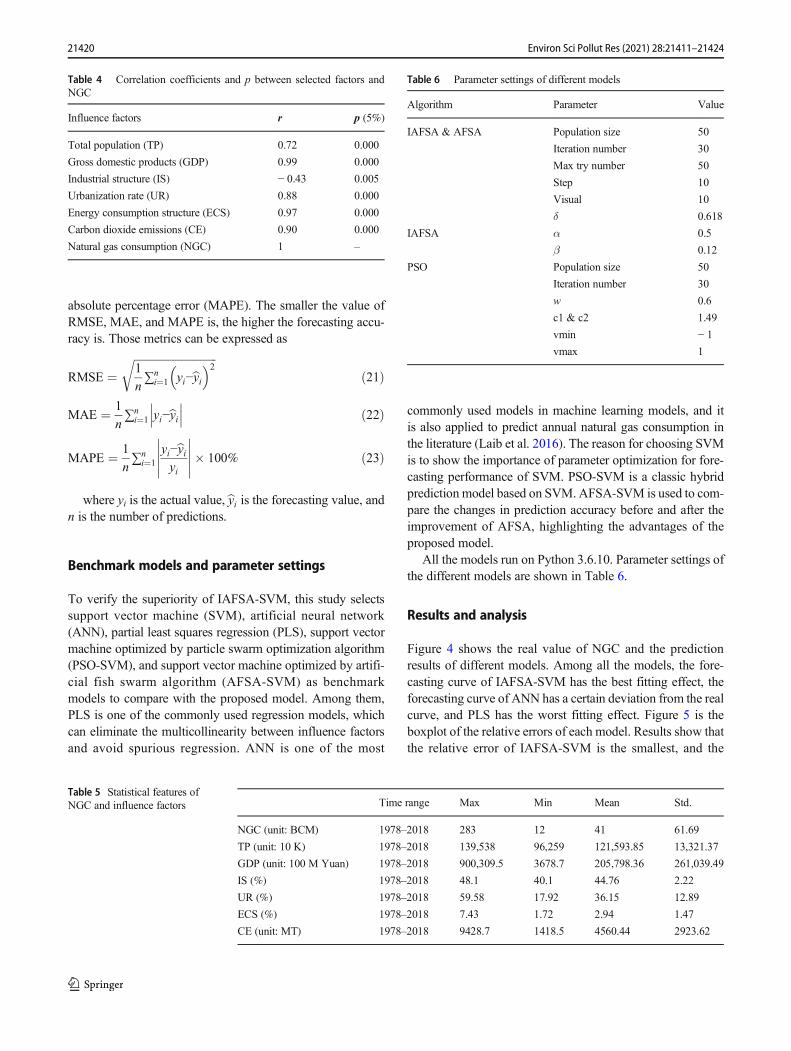
Table 4 shows that all selected factors have passed thesignificance test (p < 0.05), which means those factors arecorrelative with NGC. GDP has the largest correlation coeffi-cient (0.99), that is to say, GDP has a significant impact onNGC. The second largest one is energy consumption struc-ture, and the correlation coefficient is 0.97. Industrial structurehas a weak negative correlation with NGC.

The NGC data of China were collected from 2019 BritishPetroleum Statistical Review of World Energy (BP 2019).The data of the influence factors were collected from the2019 China Statistical Yearbook (NBSC 2019) and 2019British Petroleum Statistical Review of World Energy (BP2019). All data are annual data from 1978 to 2018, and thedetailed description is shown in Table 5. In this study, we splitthe data into two parts: training sample (1978–2012) and test-ing sample (2013–2018). The training sample is used to fit themodel, and the testing sample is used to verify the predictionaccuracy of the model.

To prevent the different dimensions of influence factorsfrom affecting the forecasting effect, all data are normalized.The formula is expressed as

X0 ¼ X−Xmin

Xmax−Xminð20Þ

where X is the original data, Xmax is the maximum value, Xmin

is the minimum value, and X′ is the normalized data, X′ ∈ [0,1].

Experimental results and discussion

Evaluation metrics

To evaluate the forecasting accuracy of models, three errorevaluation methods, widely used in previous literature, areselected as evaluation metrics, including root mean squarederror (RMSE), mean absolute error (MAE), and mean

Original data Preprocessing data

SVM forecas�ng model Predic�on results

IAFSA

Error analysis

Preprocessing module

Sigmiod func�on

Forecas�ng module evalua�on module

op�miza�on moduleInfluence

factor dataNatural gas

consump�on data

Fig. 3 Framework of NGCforecasting based on IAFSA-SVM


absolute percentage error (MAPE). The smaller the value ofRMSE, MAE, and MAPE is, the higher the forecasting accu-racy is. Those metrics can be expressed as

RMSE ¼ffiffiffiffiffiffiffiffiffiffiffiffiffiffiffiffiffiffiffiffiffiffiffiffiffiffiffiffiffiffi1

n∑n

i¼1 yi−byi� �2r

ð21Þ

MAE ¼ 1

n∑n

i¼1 yi−byi�� ð22Þ

MAPE ¼ 1

n∑n

i¼1

yi−byiyi

�� 100% ð23Þ

where yi is the actual value, byi is the forecasting value, andn is the number of predictions.

Benchmark models and parameter settings

To verify the superiority of IAFSA-SVM, this study selectssupport vector machine (SVM), artificial neural network(ANN), partial least squares regression (PLS), support vectormachine optimized by particle swarm optimization algorithm(PSO-SVM), and support vector machine optimized by artifi-cial fish swarm algorithm (AFSA-SVM) as benchmarkmodels to compare with the proposed model. Among them,PLS is one of the commonly used regression models, whichcan eliminate the multicollinearity between influence factorsand avoid spurious regression. ANN is one of the most

commonly used models in machine learning models, and itis also applied to predict annual natural gas consumption inthe literature (Laib et al. 2016). The reason for choosing SVMis to show the importance of parameter optimization for fore-casting performance of SVM. PSO-SVM is a classic hybridprediction model based on SVM. AFSA-SVM is used to com-pare the changes in prediction accuracy before and after theimprovement of AFSA, highlighting the advantages of theproposed model.

All the models run on Python 3.6.10. Parameter settings ofthe different models are shown in Table 6.

Results and analysis

Figure 4 shows the real value of NGC and the predictionresults of different models. Among all the models, the fore-casting curve of IAFSA-SVM has the best fitting effect, theforecasting curve of ANN has a certain deviation from the realcurve, and PLS has the worst fitting effect. Figure 5 is theboxplot of the relative errors of each model. Results show thatthe relative error of IAFSA-SVM is the smallest, and the

Table 4 Correlation coefficients and p between selected factors andNGC

Influence factors r p (5%)

Total population (TP) 0.72 0.000

Gross domestic products (GDP) 0.99 0.000

Industrial structure (IS) − 0.43 0.005

Urbanization rate (UR) 0.88 0.000

Energy consumption structure (ECS) 0.97 0.000

Carbon dioxide emissions (CE) 0.90 0.000

Natural gas consumption (NGC) 1 –

Table 5 Statistical features ofNGC and influence factors Time range Max Min Mean Std.

NGC (unit: BCM) 1978–2018 283 12 41 61.69

TP (unit: 10 K) 1978–2018 139,538 96,259 121,593.85 13,321.37

GDP (unit: 100 M Yuan) 1978–2018 900,309.5 3678.7 205,798.36 261,039.49

IS (%) 1978–2018 48.1 40.1 44.76 2.22

UR (%) 1978–2018 59.58 17.92 36.15 12.89

ECS (%) 1978–2018 7.43 1.72 2.94 1.47

CE (unit: MT) 1978–2018 9428.7 1418.5 4560.44 2923.62

Table 6 Parameter settings of different models

Algorithm Parameter Value

IAFSA & AFSA Population size 50

Iteration number 30

Max try number 50

Step 10

Visual 10

δ 0.618

IAFSA α 0.5

β 0.12

PSO Population size 50

Iteration number 30

w 0.6

c1 & c2 1.49

vmin − 1

vmax 1


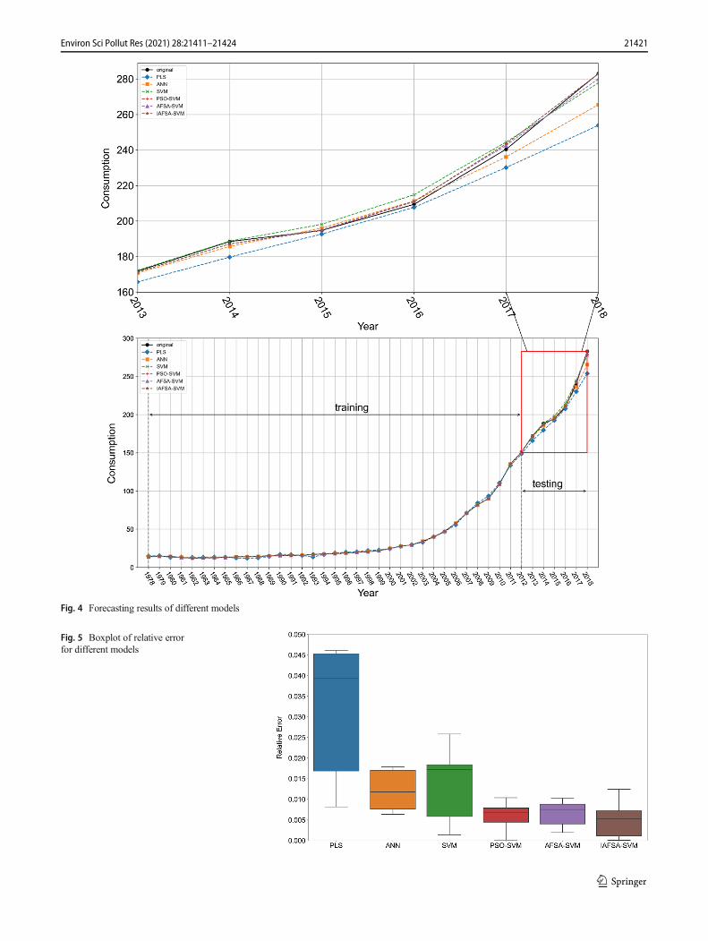
Fig. 4 Forecasting results of different models

Fig. 5 Boxplot of relative errorfor different models


relative error of PLS is the largest. The relative error of allmodels is no more than 5%.

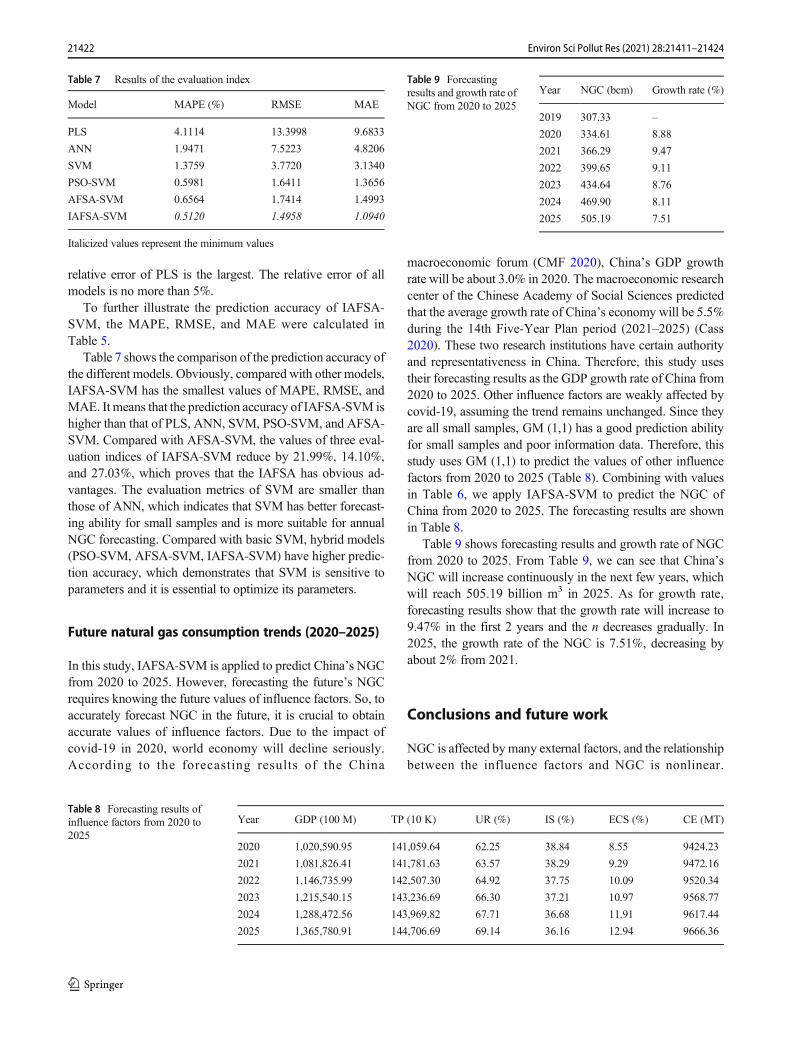
To further illustrate the prediction accuracy of IAFSA-SVM, the MAPE, RMSE, and MAE were calculated inTable 5.

Table 7 shows the comparison of the prediction accuracy ofthe different models. Obviously, compared with other models,IAFSA-SVM has the smallest values of MAPE, RMSE, andMAE. It means that the prediction accuracy of IAFSA-SVM ishigher than that of PLS, ANN, SVM, PSO-SVM, and AFSA-SVM. Compared with AFSA-SVM, the values of three eval-uation indices of IAFSA-SVM reduce by 21.99%, 14.10%,and 27.03%, which proves that the IAFSA has obvious ad-vantages. The evaluation metrics of SVM are smaller thanthose of ANN, which indicates that SVM has better forecast-ing ability for small samples and is more suitable for annualNGC forecasting. Compared with basic SVM, hybrid models(PSO-SVM, AFSA-SVM, IAFSA-SVM) have higher predic-tion accuracy, which demonstrates that SVM is sensitive toparameters and it is essential to optimize its parameters.

Future natural gas consumption trends (2020–2025)

In this study, IAFSA-SVM is applied to predict China’s NGCfrom 2020 to 2025. However, forecasting the future’s NGCrequires knowing the future values of influence factors. So, toaccurately forecast NGC in the future, it is crucial to obtainaccurate values of influence factors. Due to the impact ofcovid-19 in 2020, world economy will decline seriously.According to the forecasting results of the China

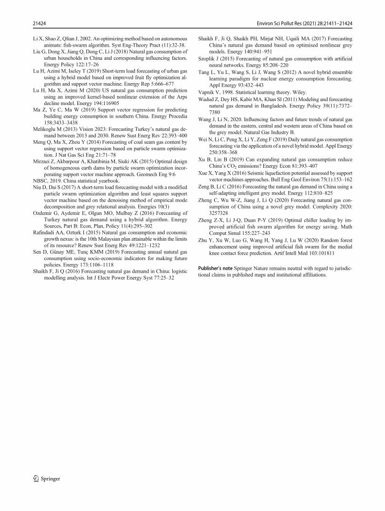
macroeconomic forum (CMF 2020), China’s GDP growthrate will be about 3.0% in 2020. The macroeconomic researchcenter of the Chinese Academy of Social Sciences predictedthat the average growth rate of China’s economy will be 5.5%during the 14th Five-Year Plan period (2021–2025) (Cass2020). These two research institutions have certain authorityand representativeness in China. Therefore, this study usestheir forecasting results as the GDP growth rate of China from2020 to 2025. Other influence factors are weakly affected bycovid-19, assuming the trend remains unchanged. Since theyare all small samples, GM (1,1) has a good prediction abilityfor small samples and poor information data. Therefore, thisstudy uses GM (1,1) to predict the values of other influencefactors from 2020 to 2025 (Table 8). Combining with valuesin Table 6, we apply IAFSA-SVM to predict the NGC ofChina from 2020 to 2025. The forecasting results are shownin Table 8.

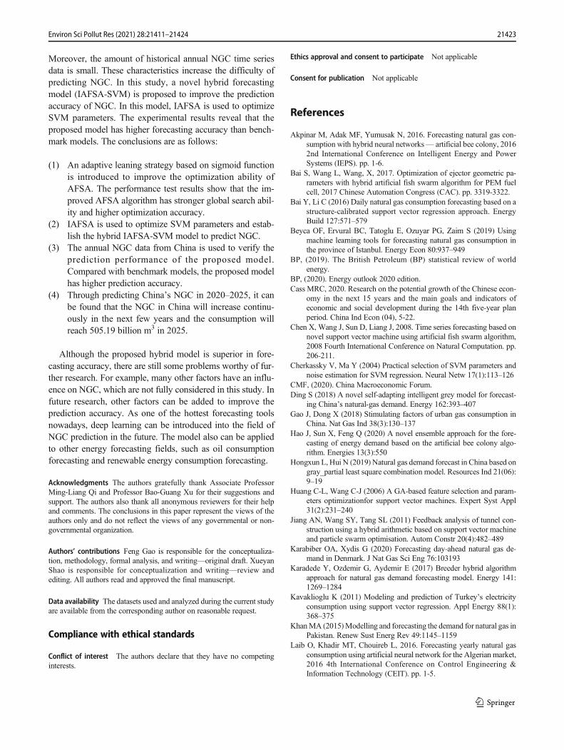
Table 9 shows forecasting results and growth rate of NGCfrom 2020 to 2025. From Table 9, we can see that China’sNGC will increase continuously in the next few years, whichwill reach 505.19 billion m3 in 2025. As for growth rate,forecasting results show that the growth rate will increase to9.47% in the first 2 years and the n decreases gradually. In2025, the growth rate of the NGC is 7.51%, decreasing byabout 2% from 2021.

Conclusions and future work

NGC is affected bymany external factors, and the relationshipbetween the influence factors and NGC is nonlinear.

Table 7 Results of the evaluation index

Model MAPE (%) RMSE MAE

PLS 4.1114 13.3998 9.6833

ANN 1.9471 7.5223 4.8206

SVM 1.3759 3.7720 3.1340

PSO-SVM 0.5981 1.6411 1.3656

AFSA-SVM 0.6564 1.7414 1.4993

IAFSA-SVM 0.5120 1.4958 1.0940

Italicized values represent the minimum values

Table 8 Forecasting results ofinfluence factors from 2020 to2025

Year GDP (100 M) TP (10 K) UR (%) IS (%) ECS (%) CE (MT)

2020 1,020,590.95 141,059.64 62.25 38.84 8.55 9424.23

2021 1,081,826.41 141,781.63 63.57 38.29 9.29 9472.16

2022 1,146,735.99 142,507.30 64.92 37.75 10.09 9520.34

2023 1,215,540.15 143,236.69 66.30 37.21 10.97 9568.77

2024 1,288,472.56 143,969.82 67.71 36.68 11.91 9617.44

2025 1,365,780.91 144,706.69 69.14 36.16 12.94 9666.36

Table 9 Forecastingresults and growth rate ofNGC from 2020 to 2025

Year NGC (bcm) Growth rate (%)

2019 307.33 –

2020 334.61 8.88

2021 366.29 9.47

2022 399.65 9.11

2023 434.64 8.76

2024 469.90 8.11

2025 505.19 7.51


Moreover, the amount of historical annual NGC time seriesdata is small. These characteristics increase the difficulty ofpredicting NGC. In this study, a novel hybrid forecastingmodel (IAFSA-SVM) is proposed to improve the predictionaccuracy of NGC. In this model, IAFSA is used to optimizeSVM parameters. The experimental results reveal that theproposed model has higher forecasting accuracy than bench-mark models. The conclusions are as follows:

(1) An adaptive leaning strategy based on sigmoid functionis introduced to improve the optimization ability ofAFSA. The performance test results show that the im-proved AFSA algorithm has stronger global search abil-ity and higher optimization accuracy.

(2) IAFSA is used to optimize SVM parameters and estab-lish the hybrid IAFSA-SVM model to predict NGC.

(3) The annual NGC data from China is used to verify theprediction performance of the proposed model.Compared with benchmark models, the proposed modelhas higher prediction accuracy.

(4) Through predicting China’s NGC in 2020–2025, it canbe found that the NGC in China will increase continu-ously in the next few years and the consumption willreach 505.19 billion m3 in 2025.

Although the proposed hybrid model is superior in fore-casting accuracy, there are still some problems worthy of fur-ther research. For example, many other factors have an influ-ence on NGC, which are not fully considered in this study. Infuture research, other factors can be added to improve theprediction accuracy. As one of the hottest forecasting toolsnowadays, deep learning can be introduced into the field ofNGC prediction in the future. The model also can be appliedto other energy forecasting fields, such as oil consumptionforecasting and renewable energy consumption forecasting.

Acknowledgments The authors gratefully thank Associate ProfessorMing-Liang Qi and Professor Bao-Guang Xu for their suggestions andsupport. The authors also thank all anonymous reviewers for their helpand comments. The conclusions in this paper represent the views of theauthors only and do not reflect the views of any governmental or non-governmental organization.

Authors’ contributions Feng Gao is responsible for the conceptualiza-tion, methodology, formal analysis, and writing—original draft. XueyanShao is responsible for conceptualization and writing—review andediting. All authors read and approved the final manuscript.

Data availability The datasets used and analyzed during the current studyare available from the corresponding author on reasonable request.

Compliance with ethical standards

Conflict of interest The authors declare that they have no competinginterests.

Ethics approval and consent to participate Not applicable

Consent for publication Not applicable

References

Akpinar M, Adak MF, Yumusak N, 2016. Forecasting natural gas con-sumption with hybrid neural networks— artificial bee colony, 20162nd International Conference on Intelligent Energy and PowerSystems (IEPS). pp. 1-6.

Bai S, Wang L, Wang, X, 2017. Optimization of ejector geometric pa-rameters with hybrid artificial fish swarm algorithm for PEM fuelcell, 2017 Chinese Automation Congress (CAC). pp. 3319-3322.

Bai Y, Li C (2016) Daily natural gas consumption forecasting based on astructure-calibrated support vector regression approach. EnergyBuild 127:571–579

Beyca OF, Ervural BC, Tatoglu E, Ozuyar PG, Zaim S (2019) Usingmachine learning tools for forecasting natural gas consumption inthe province of Istanbul. Energy Econ 80:937–949

BP, (2019). The British Petroleum (BP) statistical review of worldenergy.

BP, (2020). Energy outlook 2020 edition.Cass MRC, 2020. Research on the potential growth of the Chinese econ-

omy in the next 15 years and the main goals and indicators ofeconomic and social development during the 14th five-year planperiod. China Ind Econ (04), 5-22.

Chen X, Wang J, Sun D, Liang J, 2008. Time series forecasting based onnovel support vector machine using artificial fish swarm algorithm,2008 Fourth International Conference on Natural Computation. pp.206-211.

Cherkassky V, Ma Y (2004) Practical selection of SVM parameters andnoise estimation for SVM regression. Neural Netw 17(1):113–126

CMF, (2020). China Macroeconomic Forum.Ding S (2018) A novel self-adapting intelligent grey model for forecast-

ing China’s natural-gas demand. Energy 162:393–407Gao J, Dong X (2018) Stimulating factors of urban gas consumption in

China. Nat Gas Ind 38(3):130–137Hao J, Sun X, Feng Q (2020) A novel ensemble approach for the fore-

casting of energy demand based on the artificial bee colony algo-rithm. Energies 13(3):550

Hongxun L, Hui N (2019) Natural gas demand forecast in China based ongray_partial least square combination model. Resources Ind 21(06):9–19

Huang C-L, Wang C-J (2006) A GA-based feature selection and param-eters optimizationfor support vector machines. Expert Syst Appl31(2):231–240

Jiang AN, Wang SY, Tang SL (2011) Feedback analysis of tunnel con-struction using a hybrid arithmetic based on support vector machineand particle swarm optimisation. Autom Constr 20(4):482–489

Karabiber OA, Xydis G (2020) Forecasting day-ahead natural gas de-mand in Denmark. J Nat Gas Sci Eng 76:103193

Karadede Y, Ozdemir G, Aydemir E (2017) Breeder hybrid algorithmapproach for natural gas demand forecasting model. Energy 141:1269–1284

Kavaklioglu K (2011) Modeling and prediction of Turkey’s electricityconsumption using support vector regression. Appl Energy 88(1):368–375

KhanMA (2015)Modelling and forecasting the demand for natural gas inPakistan. Renew Sust Energ Rev 49:1145–1159

Laib O, Khadir MT, Chouireb L, 2016. Forecasting yearly natural gasconsumption using artificial neural network for the Algerian market,2016 4th International Conference on Control Engineering &Information Technology (CEIT). pp. 1-5.


LiX, Shao Z, QIian J, 2002. An optimizingmethod based on autonomousanimats: fish-swarm algorithm. Syst Eng-Theory Pract (11):32-38.

Liu G, Dong X, Jiang Q, Dong C, Li J (2018) Natural gas consumption ofurban households in China and corresponding influencing factors.Energy Policy 122:17–26

Lu H, Azimi M, Iseley T (2019) Short-term load forecasting of urban gasusing a hybrid model based on improved fruit fly optimization al-gorithm and support vector machine. Energy Rep 5:666–677

Lu H, Ma X, Azimi M (2020) US natural gas consumption predictionusing an improved kernel-based nonlinear extension of the Arpsdecline model. Energy 194:116905

Ma Z, Ye C, Ma W (2019) Support vector regression for predictingbuilding energy consumption in southern China. Energy Procedia158:3433–3438

Melikoglu M (2013) Vision 2023: Forecasting Turkey’s natural gas de-mand between 2013 and 2030. Renew Sust Energ Rev 22:393–400

Meng Q, Ma X, Zhou Y (2014) Forecasting of coal seam gas content byusing support vector regression based on particle swarm optimiza-tion. J Nat Gas Sci Eng 21:71–78

Mirzaei Z, Akbarpour A, Khatibinia M, Siuki AK (2015) Optimal designof homogeneous earth dams by particle swarm optimization incor-porating support vector machine approach. Geomech Eng 9:6

NBSC, 2019. China statistical yearbook.Niu D, Dai S (2017) A short-term load forecasting model with a modified

particle swarm optimization algorithm and least squares supportvector machine based on the denoising method of empirical modedecomposition and grey relational analysis. Energies 10(3)

Ozdemir G, Aydemir E, Olgun MO, Mulbay Z (2016) Forecasting ofTurkey natural gas demand using a hybrid algorithm. EnergySources, Part B: Econ, Plan, Policy 11(4):295–302

Rafindadi AA, Ozturk I (2015) Natural gas consumption and economicgrowth nexus: is the 10thMalaysian plan attainable within the limitsof its resource? Renew Sust Energ Rev 49:1221–1232

Sen D, Günay ME, Tunç KMM (2019) Forecasting annual natural gasconsumption using socio-economic indicators for making futurepolicies. Energy 173:1106–1118

Shaikh F, Ji Q (2016) Forecasting natural gas demand in China: logisticmodelling analysis. Int J Electr Power Energy Syst 77:25–32

Shaikh F, Ji Q, Shaikh PH, Mirjat NH, Uqaili MA (2017) ForecastingChina’s natural gas demand based on optimised nonlinear greymodels. Energy 140:941–951

Szoplik J (2015) Forecasting of natural gas consumption with artificialneural networks. Energy 85:208–220

Tang L, Yu L, Wang S, Li J, Wang S (2012) A novel hybrid ensemblelearning paradigm for nuclear energy consumption forecasting.Appl Energy 93:432–443

Vapnik V, 1998. Statistical learning theory. Wiley.Wadud Z, Dey HS, Kabir MA, Khan SI (2011) Modeling and forecasting

natural gas demand in Bangladesh. Energy Policy 39(11):7372–7380

Wang J, Li N, 2020. Influencing factors and future trends of natural gasdemand in the eastern, central and western areas of China based onthe grey model. Natural Gas Industry B.

Wei N, Li C, Peng X, Li Y, Zeng F (2019) Daily natural gas consumptionforecasting via the application of a novel hybridmodel. Appl Energy250:358–368

Xu B, Lin B (2019) Can expanding natural gas consumption reduceChina’s CO2 emissions? Energy Econ 81:393–407

Xue X, Yang X (2016) Seismic liquefaction potential assessed by supportvector machines approaches. Bull Eng Geol Environ 75(1):153–162

Zeng B, Li C (2016) Forecasting the natural gas demand in China using aself-adapting intelligent grey model. Energy 112:810–825

Zheng C, Wu W-Z, Jiang J, Li Q (2020) Forecasting natural gas con-sumption of China using a novel grey model. Complexity 2020:3257328

Zheng Z-X, Li J-Q, Duan P-Y (2019) Optimal chiller loading by im-proved artificial fish swarm algorithm for energy saving. MathComput Simul 155:227–243

Zhu Y, Xu W, Luo G, Wang H, Yang J, Lu W (2020) Random forestenhancement using improved artificial fish swarm for the medialknee contact force prediction. Artif Intell Med 103:101811

Publisher’s note Springer Nature remains neutral with regard to jurisdic-tional claims in published maps and institutional affiliations.


Documents

Forecasting annual natural gas consumption via the