Embed Size (px)
Citation preview
8/13/2019 Forecasting Demand for Petroleum Products in Ghana EDITED
http://slidepdf.com/reader/full/forecasting-demand-for-petroleum-products-in-ghana-edited 1/20
Journal of Economics and Sustainable Development www.iiste.org
1
Forecasting Demand for Petroleum Products in Ghana
Using Time Series Models
Godfred Kwame Abledu(PhD)1*, Boakye Agyemang2,and Semevor Reubin3
1. School of Applied Science and Technology, Koforidua Polytechnic, PO Box 981,Koforidua, Ghana
2. Statistics Department, Koforidua Polytechnic, PO Box 981, Koforidua, Ghana
3. Applied Mathematics Department, Koforidua Polytechnic, PO Box 981, Koforidua,Ghana
* E-mail of the corresponding author: [email protected]
Abstract
The objective of this study was to forecast and analyse the demand for petroleum
products in Ghana using annual data from 2000-2010. It focused on studying the feasibilityforecast using nested conditional mean (ARMA) and conditional variance (GARCH, GJR,EGARCH) family of models under such volatile market conditions. A regression based forecastfiltering simulation was proposed and studied for any improvements in the forecast results.
Keywords: time Series models, regression model, forecast filtering, petroleum products,stationarity of time Series data.
1. Introduction
The demand for petroleum has increased in the last decade all over the world includingthe United States, Middle Eastern nations, and other Asian nations, which has contributed in thehigh prices. The demand for petroleum products in India has been increasing at a rate higher thanthe increase of domestic availability (Banapurmath, et. al., 2011). At the same time, there iscontinuous pressure on emission control through periodically tightened regulations particularlyin metropolitan cities. Over the period 1980-2008, the price of crude oil had fluctuatedsignificantly, with a mean, minimum and maximum values of $ 32.31 (bbl), $ 12.72 (bbl) and $140 (bbl) respectively(WAMA(2008). The above statistics, in addition to a standard deviation of 17.08 over the sample period show that the prices of crude have always been characterized withsevere instability. Monthly fluctuations have in fact been more severe than these annual trends,with the price of crude oil reaching $140 (bbl) in July 2008. Such instability in the prices of crude oil is bound to cause macroeconomic distortions, especially in net-oil importing countries,like some ECOWAS countries (WAMA, 2008).
Ghana’s demand for crude oil and refined petroleum products has also been growing overthe past decade, and, the country’s demand for oil increased dramatically surprising many energy
analysts. This growth has been driven by socio-economic and technical factors that have
8/13/2019 Forecasting Demand for Petroleum Products in Ghana EDITED
http://slidepdf.com/reader/full/forecasting-demand-for-petroleum-products-in-ghana-edited 2/20
Journal of Economics and Sustainable Development www.iiste.org
2
influenced each category of final energy use. These changing petroleum requirements are closelyrelated to its high rates of growth in economic output and personal incomes. The growth inincomes and the accompanying changes in petroleum demand are themselves driven by anongoing population shift from rural to urban areas. That growing urban population is demandingnew vehicles and new roads, raising the demand for energy in the transportation sector. The
growth in output in the industrial sector is driving the high demand for petrochemical feedstocks, including naphtha-based petrochemicals, which are similar in composition to motorgasoline. Fluid catalytic cracking of heavy ends to high-value liquid fuels is a common unitoperation in oil refineries (Khan, et al., 2011). In this process, the heavy feedstock that containssulfur is cracked to light products
At the core of the development of every nation is petroleum. Currently, petroleum isamong the most important natural resources. Every nation uses petroleum products such asgasoline, jet fuel, liquefied petroleum gas and diesel to run cars, trucks, aircraft and othervehicles. There is therefore the need to build stocks to meet the seasonal demands. In the longterm, blending non-petroleum additives into petroleum products such as ethanol or other
oxygenating agents into gasoline will be necessary to reduce crude oil demand. Efficient refiningcapacity is a requirement to meet the demand of the nations. The past few years have witnessedan increased impetus toward renewable energy to replace fossil fuels that has been driven bothby environmental and national security concerns (Hensel, 2011).
Many researchers analyzing the demand for petroleum products have looked at theaggregate consumption of petroleum. Sa'ad(2009), used annual time series data for the period1973 to 2007 in two econometric techniques namely the structural time series model (STSM) andunrestricted error correction model (UECM) to estimate demand for petroleum products. Theresults from both models revealed that the demand for petroleum products is price inelastic. Therobust optimization methodology is applied to deal with uncertainties in the prices of saleable
products, operating costs, product demand, and product yield in the context of refineryoperational planning (Leiras, et al , 2010 and Munim, et al.,2010
MATERIALS AND METHOD
Conditional mean models were used to forecast mean while the conditional variancemodels were used for forecasting variance or volatility in the demand for oil. In this study, thenesting of these two models was used first to forecast the conditional mean and then theconditional variance was estimated to get the value of forecast demands for oil(Shrivastava,2009). After analysis of data for quarter 1 (Q1r) and quarter 2 (Q2r), ARMA(2,2) models hadbeen found most appropriate for forecasting mean, hence ARMA(2,2) and(GARCH(1,1)/GJR(1,1) /EGARCH(1,1)) were used for forecasting oil demand for 2012 and
2013.
The conditional mean and variance models have been viewed from a linear filteringperspective, and then the application of the iterated conditional expectations to the recursiveequations was conducted, one forecast period at a time (Dhar, et. al. , 2009). For example for
8/13/2019 Forecasting Demand for Petroleum Products in Ghana EDITED
http://slidepdf.com/reader/full/forecasting-demand-for-petroleum-products-in-ghana-edited 3/20
Journal of Economics and Sustainable Development www.iiste.org
3
forecasting demand for the second quarter (Q2), demand data were taken of quarter 1 (Q1) andforecast using above defined method has been done. Using observed quarter 2(Q2) demand asdependent variable and (ARMA/GARCH) forecast as independent variable regression model wasobtained. Calculation of quarter 3 demand (Q3r) using observed data of Q2 was obtained usingnested models and the regression model obtained in the previous step was used to filter quarter 3
(Q3) demand forecast.
Conditional variance models (Shrivastava, 2009), unlike the traditional or extreme valueestimators, incorporate time varying characteristics of second moment/volatility explicitly. Thefollowing models fall into the category of conditional volatility models(Hull, 2006):
i. ARCH (m) Model (Auto Regressive Conditional Heteroscedasticity)ii. EWMA Model (Exponentially Weighted Moving Average Model)
iii. GARCH(a,b)Model(Generalized Autoregressive Conditional Heteroscedasticity).iv. EGARCH Model.
The stationarity was tested using ADF test with and without drift and trend, the AR(p)was determined using PACF and MA(q) was determined using ACF. The number of laggedterms to be included in the model was identified based on the minimum value of AIC and SBCcriteria. The ARMA model was tested for ARCH effects using the ARCH LM test and themeasures of performance were calculated for the static and dynamic forecasts made for the out-sample period. The in-sample data constituting 80% was used for estimating the coefficients of the parameters and 20% the out-of- sample data was forecasted.
The forecasted results from random walk model, ARMA, ARMA-GARCH, ARMA-EGARCH models using static and dynamic forecasting were compared based on the predictivepower using the three forecasting accuracy measures: Root Mean Square Error, Mean AbsoluteError and Thiel Inequality Coefficient. Theil’s U statistic was rescaled and decomposed into 3proportions of inequality – bias, variance and covariance – such that bias + variance +
covariance = 1 and these measures were also calculated.
1.1. Autoregressive Moving Average( ARMA )Models
The Autoregressive Moving Average (ARMA) Models have been used by manyresearcher for forecasting(Shrivastava, et, al. , 2010; Abu and Behrooz, 2011) . Given a time
series of data t Z , the ARMA model is a tool for understanding and, perhaps, predicting future
values in this series. The model consists of two parts, an autoregressive (AR) part and a movingaverage (MA) part. The model is usually then referred to as the ARMA (a, b) model where “a” isthe order of the autoregressive part and “b” is the order of the moving average part. The notationARMA (a, b) refers to the model with “a” autoregressive terms and “b” moving-average terms.
This model contains the AR(a) and MA(b) models. A time series t Z follows an ARMA (1, 1)
model if it satisfies
b
i
it iit
a
i
it Z k Z 11
1 ωαβω , where { t ω } is a white noise series. The
above equation implies that the forecast value is depended on the past value and previous shocks.
8/13/2019 Forecasting Demand for Petroleum Products in Ghana EDITED
http://slidepdf.com/reader/full/forecasting-demand-for-petroleum-products-in-ghana-edited 4/20
Journal of Economics and Sustainable Development www.iiste.org
4
The notation MA(b) which refers to the moving average model of order b is written as
b
i
it it t k Z 1
ωαω and the notation AR(a) which refers to the autoregressive model of order
a, is written as it
a
i
it Z k Z
1
1 βω where thebαα ,...,1
are the parameters of the model, μ is
the expectation of Zt (often assumed to equal to 0), and thebt t ωω ,..., are again, white noise error
terms.
The Autoregressive Moving Average model(ARMA) is a method which can be usedwhen the time series variable is related to past values of itself. By regressing Zt on somecombination of its past values, we are able to derive a forecasting equation. We expect theautoregressive technique to perform reasonably well for a time series that:
1. Is not extremely volatile and does not contain extreme amounts of randommovement.
2. Requires “q” short-term or medium- term forecast, that is less than two years
The fact that the autoregressive procedure does not perform well on a time series is not aserious disadvantage. Practically all forecasting techniques perform poorly in this situation.Suppose we want to predict the values of Z t using the previous observation, we use the expanded
equation: 22110 t t t Z b Z bb Z , where t takes the values = 3, 4, 5, …. The values 0b , 1b , and
2b are the least squares regression estimates obtained from any multiple linear regression. There
are two predictor variables here, the lagged variables, 1t Z and 2t Z . The above equation is a
second order autoregressive equation because it uses the two lagged terms. In general, the ath –
order autoregressive equation is given as :^
22110 ... at at t t Z b Z b Z bb Z , and
,...2,1 aat
The assumption underlying the ARMA model is that the future value of a variable is alinear function of past observations and random errors. In this model it is possible to find anadequate description of data set. This method consists of four steps:
1. Model identification,2. Parameter estimation,3. Diagnostic checking and4. Forecasting.In the identification step, it can be seen that a model generated from an ARMA process may
contain some autocorrelation properties, so there will be some potential models that can fit thedata set but the best fitted model is selected according to AIC information criteria. Stationarity isa necessary condition in building an ARMA model used for forecasting, so data transformation isoften required to make the time series to be stationary. In this study, the unit root test, known as
8/13/2019 Forecasting Demand for Petroleum Products in Ghana EDITED
http://slidepdf.com/reader/full/forecasting-demand-for-petroleum-products-in-ghana-edited 5/20
Journal of Economics and Sustainable Development www.iiste.org
5
the Dickey and Fuller test (Shrivastava, et, al., 2010; Gujarati, 2006; Abu and Behrooz, 2011 ), isused to test the stationarity of the time series.
Based on the result obtained, the data set is stationary at first difference even with theexistence of structural break. Once a tentative model is obtained, estimation of the model
parameters is applicable. The parameters are estimated such that an overall measure of errors isminimized. The third step is diagnostic checking for model adequacy. Autocorrelation and alsoserial correlation of the residuals are used to test the goodness of fit of the tentatively obtainedmodel to the original data. When the final model is approved then it will be used for predictionof future values of the oil demand.
1.2. The ARCH/GARCH Models
The first model that provides a systematic framework for volatility modeling is the ARCH
model of Engle (Gujarati, 2006). The basic idea of the ARCH model is that the shock αt of an
asset return is serially uncorrected but dependent; also the dependence of αt can be described by
a simple quadratic function of its lagged values. Specifically, an ARCH (m) model assumes that
t t t a σε ,
2 2 2
0 1 1 .....t t m t ma aσ α α α (Gujarati, 2006), where t ε is a sequence of
independent and identically distributed (i.i.d.) random variables with mean zero and variance 1,
0 0α and 0i
α for 0i . The coefficient iα must satisfy some regularity condition to ensure
that the unconditional variance of t a is finite. In practices, t ε is often assumed to follow the
standard normal or a standardized student t distribution or a generalized error distribution.
GARCH models are used as a successful treatment to the financial data which oftendemonstrate time-persistence, volatility clustering and deviation from the normal distribution.Among the earliest models is Engel (1982) linear ARCH model, which captures the time varying
feature of the conditional variance. Bollerslev (1986) develops Generalized ARCH (GARCH)model, allowing for persistency of the conditional variance and more efficient testing. Engle andBollerslev (1986) invent the Integrated GARCH (IGARCH) model that provides consistentestimation under the unit root condition. Engle, Lilien, and Robins (1987) design the ARCH-in-Mean (ARCH-M) model to allow for time varying conditional mean. Nelson’s (1990a & b)Exponential GARCH (EGARCH) model allows asymmetric effects and negative coefficients inthe conditional variance function.
The leveraged GARCH (LGARCH) model documented in Glosten, Jagannathan andRunkle (1993) takes into account the asymmetric effects of shocks from different directions.Since their introduction by Engle (1982), Autoregressive Conditional Heteroskedastic (ARCH)models and their extension by Bollerslev (1986) to generalised ARCH (GARCH) processes,
GARCH models have been used widely by practitioners. At a first glance, their structure mayseem simple, but their mathematical treatment has turned out to be quite complex. Although theARCH is simple, it often requires many parameters to adequately describe the volatility processof an asset return some alternative models must be sought. Shrivastava, et al. (2010) andHull(2006) proposed a useful extension known as the generalized ARCH (GARCH) model. An
8/13/2019 Forecasting Demand for Petroleum Products in Ghana EDITED
http://slidepdf.com/reader/full/forecasting-demand-for-petroleum-products-in-ghana-edited 6/20
Journal of Economics and Sustainable Development www.iiste.org
6
important feature of GARCH-type models is that the unconditional volatility σ depends on the
entire sample, while the conditional volatilities t σ are determined by model parameters and
recent return observations.
Let t t ε be a sequence of independent and identically distributed (i.i.d.) random
variables, and let 1,2,3,..., p and 0o p . Further, let 0 0α , 1 1, ..., 0 pα α ,
0 pα , 1 1,..., 0qβ β and 0qβ be non-negative parameters. A GARCH(p, q) process
t X t with volatility process is t t σ is then a solution to the equations:
t t t X σ ε
,t (1)
2 2 2
1 1
1 1
p q
t t i t j t
i j
X σ α α β σ
,t (2)
where the process t t σ is non-negative. The sequence t t ε is referred to as the
driving noise sequence. GARCH (p, 0) processes are called ARCH (p) processes. The case of aGARCH (0, q) process is excluded since in that case, the volatility equation (2) decouples fromthe observed process and the driving noise sequence.
It is a desirable property thatt σ should depend only on the past
innovations ( )t h hε , that is, it is measurable with respect to σ algebra generated by
( )t h hε . If this condition holds, we shall call the GARCH (p, q) process causal. Then
t X is measurable with respect to σ algebra0( : )t h hσ ε , generated by 0( )t h hε .
Also,t
σ is independent of 0
( )t h hε , andt
X is independent of ( : )t h hσ ε , for
fixed t . The requirement that all the coefficients 1,..., pα α and1,..., qβ β are non-negative ensures
that2σ is non-negative, so that
t σ can indeed be defined as the square root of 2σ .
Equation(1) is the mean equation and is specified as an AR(p) process.
Equation (2) is the conditional variance equation and it is specified as the GARCH(1,
1) process. Conditional variance models (Shrivastava, 2009), unlike the traditional or extremevalue estimators, incorporate time varying characteristics of second moment/volatility explicitly.By successively substituting for the lagged conditional variance into equation(2), the
following expression is obtained:
201 111
t i t iih
αα β ε
β
(3)
8/13/2019 Forecasting Demand for Petroleum Products in Ghana EDITED
http://slidepdf.com/reader/full/forecasting-demand-for-petroleum-products-in-ghana-edited 7/20
Journal of Economics and Sustainable Development www.iiste.org
7
An ordinary sample variance would give each of the past squares an equalweight rather than declining weights. Thus the GARCH variance is like a sample
variance but it emphasizes the most recent observations. Sincet h is the one period
ahead forecast variance based on past data, it is called the conditional variance. The
squared residual is given by:
2
t t t v hε (4)
Equation (4) is by definition unpredictable based on the past. Substituting
equation (4) into equation(2) yields an alternative expression as follows:
2 2
1 1 1( )t t t t v vε ω α β ε β (5)
From the structure of the model, it is seen that large past squared shocks 2
1
m
t i ia
imply
a large conditional variance 2
t σ for the innovation t a
.
Consequently, t a tends to assume a large
value (in modulus). This means that, under the ARCH framework, large shock tend to befollowed by another shock; because a large variance does not necessarily produce a largerealization. It only says that the probability of obtaining a large variate is greater than that of asmaller variance. To understand the ARCH models, it pays to carefully study ARCH (I) model
t t t a σε ,
2 2
0 1 1,t t aσ α α where 0 0α and 0
I α . The unconditional mean of t a remains
zero because
1 / 0t t t t t E a E E a F E E σ ε (6)
The conditional variance if at can be obtained as
2 2 2 2
1 0 1 1 0 1 1var / .t t t t t t a E a E E a F E a E aα α α α
Because t a is a stationary process with 2
1 0t E a 2
1 1var vart t t a a E a .
Therefore, we
have 0 1var vart t a aα α and 0
1
var .1
t a α
α
Since the variance of t
a must be positive,
we require 10 1α . In some applications, we need higher order moments of t a to exist and,
hence, 1α must also satisfy some additional constraints. For instance, to satisfy its tail behavior,
we require that the fourth moment of t a is finite. Under the normality assumption, we have
2 2
4 2 2
1 1 0 1 1 / 3 / 3t t t t t E a F E a F aα α (Brockwell and Davis, 1996).
Therefore , 2
4 4 2 2 2 2 4
1 0 1 1 0 0 1 1 1 1 / 3 3 2t t t t t t
E a E E a F E a E a aα α α α α α
8/13/2019 Forecasting Demand for Petroleum Products in Ghana EDITED
http://slidepdf.com/reader/full/forecasting-demand-for-petroleum-products-in-ghana-edited 8/20
Journal of Economics and Sustainable Development www.iiste.org
8
If t a is fourth – order stationary with
4
4 t m E a , then we have
2
4 0 0 1 1 43 2 vart m a mα α α α
2 210 1 4
1
3 1 2 31
mαα αα
Consequently
2
0 1
4 2
1 1
3 1.
1 1 3m
α α
α α
This result has two important implications: since the fourth moment of t a is positive, we
see that 1α must also satisfy the condition 3
11 3 0;α that is, 2
110
3α ; and the
unconditional Kurtosis of t a is
24 2
20 1 1 1
2 2 2 320 11 1
1 1 13 31 31 1 3var
t
t
E a
a
α α α αα αα α
(7)
Thus, the excess of t a is positive and the tail distribution of t a is heavier than that of a
normal distribution. In other words, the shock t a of a conditional Gaussian ARCH (I) model is
more likely than Gaussian white noise series to produce “outcome”. This is in agreement with
the empirical finding that “outliers” appear more often in asset returns than that implied by an iidsequence of normal random variates. These properties continue to hold for general ARCHmodels, but the formula becomes more complicated for higher order ARCH models.
The condition 0i
α in 2 2 2
0 1 1 ....t t m t ma aσ α α α can be related. It is a condition to
ensure that the conditional variance2
t σ is positive for all t. The model has some weakness: itassume that positive and negative shocks have the same effects on volatility because it dependson the square of the previous shocks. In practices it is well known that price of a financial assetresponds differently to positive and negative shocks.
The ARCH model is rather restrictive. For instance, 2
1α of an ARCH (I) model must be
in the interval 103
if the series has a finite fourth moment. The constraint becomes
complicated for higher order ARCH models. In limits, the ability of ARCH models withGaussian innovations is to capture excess kurtosis. The ARCH model does not provide any newinsight for understanding the sources of variation of a financial time series. It merely provides amechanical way to describe the behavior of the conditional variation. It gives no indications of what causes such behavior to occur. ARCH models are likely to over predict the volatilitybecause they respond slowly to large isolated shocks to the return series(Brockwell and Davis,1996).
8/13/2019 Forecasting Demand for Petroleum Products in Ghana EDITED
http://slidepdf.com/reader/full/forecasting-demand-for-petroleum-products-in-ghana-edited 9/20
Journal of Economics and Sustainable Development www.iiste.org
9
1.3. The EGARCH Model
This model is used to allow for symmetric effects between positive and negative assetreturns. An EGARCH (m, s) model can be written as (Dhar, et. Al. , 2009).
t t t a σε ,
12 1 1
0 1
1
1 ...
1 ....
s
s
t t m
m
B B In g B B
β βσ α εα α
(8)
wher 0α is a constant, B is the back-shift (or lag) operator such that 1t t Bg gε ε and
11 ... B s Bβ β are polynomials with zeros outside the unit circle and have no common
factors. By outside the unit circle, we mean that absolute values of the zeros are greater than 1.
Here, it is understood that 0iα for i > m and 0 jβ for j > s. The latter constraint on αi and β i
implies that the unconditional variance αt is finite, whereas its conditional variance 2
t σ evolves
over time, and t ε is often assumed to be a standard normal standardized student-t distribution or
generalized error distribution:
2 2 20 1
1 1
m m
t i t j t j
i i
σ α α α β σ
(9)
reduces to a pure ARCH (m) model if S=0.The αi and β i are referred to as ARCH and GARCH parameters respectively. The
unconditional mean of 2( )t In σ is 0α . It uses logged conditional variance to relax the positiveness
constraint of model coefficients. The use of ( )t g ε enables the model to respond asymmetrically
to the positive and negative lagged values of αt . The model is nonlinear if 0θ . Since negativeshocks tend to have larger impacts, we expect θ to be negative. For higher order EGARCHmodel, the nonlinearity becomes much more complicated. This model can be used to obtainmultistep ahead volatility forecasts.
1.4. Fitting the Parameters of the ModelOnce a model is selected and data are collected, it is the job of the researcher to estimate
the parameters of the Model. These are values that best fit the historical data. It is hypothesizedthat the resulting model will provide a prediction of the future observation. It is alsohypothesized that all values in a given sample are equal.
The time series model includes one or more parameters. We identify the estimated values
with a hat. For instance, the estimated value of β is denoted .β
The procedure also provide
estimates of the standard deviation of the noise, εσ .
1.5. Forecasting from The ModelThe main purpose of modeling a time series is to make forecasts which are then used directlyfor making decisions. In this analysis, we let the current time be T, and assume that the demandfor periods 1 through T are known. We now want to forecast the demand for the period (T+ς ).
8/13/2019 Forecasting Demand for Petroleum Products in Ghana EDITED
http://slidepdf.com/reader/full/forecasting-demand-for-petroleum-products-in-ghana-edited 10/20
Journal of Economics and Sustainable Development www.iiste.org
10
The unknown demand is the random variable X(T+ς )., and its realization is x (T+ ς ).. Our
forecast for the realization is T x
ς .
1.6. Measuring the Accuracy of the ModelThe forecast error is the difference between the realization and the forecast. Thus
eς = x(T+ς )...- T
x ς . (10)
Assuming the model is correct, then we have
ςe = [ ] E X T T
xες ς ς (11)
We investigate the probability distribution of the error by computing its mean and
variance. One desirable characteristics of the forecast T x ς is that it is unbiased. For an unbiasedestimate, the expected value of the forecast is the same as the expected value of the time series.
Because t ε is assumed to have a mean of zero, an unbiased forecast implies ][ ςε E . The fact that
the noise in independent from one period to the next period means that the variance of the error
is: [ ] { [ ] } [ ]t T T T Var Var E X x Var
ς ς ςε ε and
2)()( 22 σςσςσε
E
. (12)
2. DATA ANALYSIS AND RESULTS
2.1. Data and method of analysis
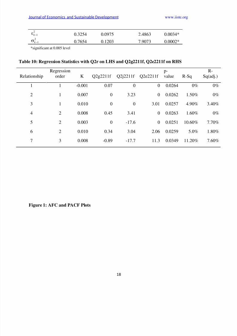
The data for the study was obtained from Tema Oil refinery. The AFC and the PACF of the time series are shown in Figure 1. The PACF shows a single spike at the first lag and the
ACF shows a tapering pattern. The positive, geometrically decaying pattern of the AFC, coupledwith single significant coefficient 11 strongly suggest an AR(1){=ARMA(1,0)} process.
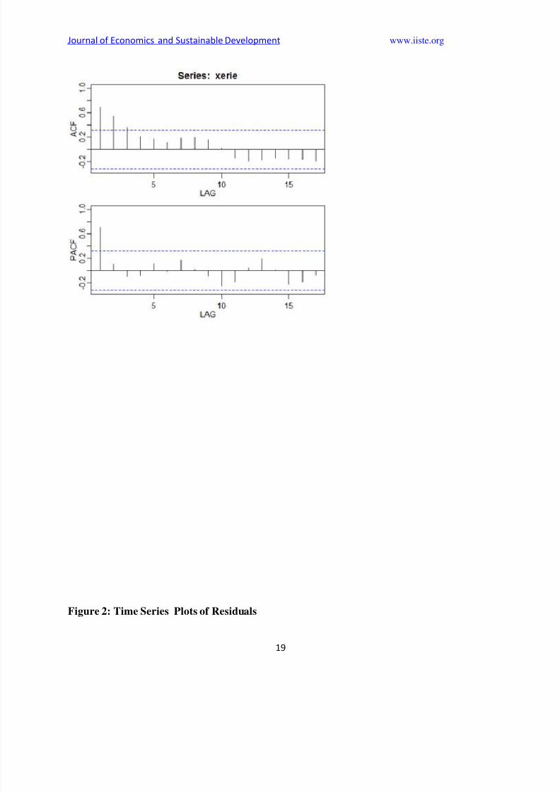
The time series plot(Figure 2) of the standardized residuals mostly indicates that there is notrend in the residuals, no outliers, and in general, no changing variance across time. The ACF of the residuals shows no significant autocorrelations, an indication of a good result. The Q-Q plotis a normal probability plot. It doesn’t look too bad, so the assumption of normally distributed
residuals looks okay. The bottom plot gives p-values for the Ljung-Box-Pierce statistics for eachlag up to 20. These statistics consider the accumulated residual autocorrelation from lag 1 up toand including the lag on the horizontal axis. The dashed blue line is at 0.05. All p-values areabove it indicating that this is a good result
The time series data ranged from January 2000 until December 2012. The coefficient of variation (V) was used to measure the index of instability of the time series data. The coefficientof variation (V) is defined as:
V Y
(13)
8/13/2019 Forecasting Demand for Petroleum Products in Ghana EDITED
http://slidepdf.com/reader/full/forecasting-demand-for-petroleum-products-in-ghana-edited 11/20
Journal of Economics and Sustainable Development www.iiste.org
11
where σ is the standard deviation and
1
1 n
t
t
Y Y n
(14)
is the mean of petroleum prices changes.
A completely stable data has V = 1, but unstable data are characterized by a V>1(Telesca et al., 2008). Regression analysis was used to test whether trends and seasonal factorsexist in the time series data. The existence of linear trend factors was tested through thisregression equation:
0 1Y T , 20,WN (15)
Stationarity is tested using unit root test. The stochastic time series of interest is Zt.
Taking the first difference we have the following: µ 1321 t t Z A A A Z where t Z is the first
difference, t is the trend variable taking on the values from 1, 2, 3, …, n. and Z t-1 is the oneperiod lagged value of the variable Z. The null hypothesis is that A3, the coefficient of Zt-1 iszero. That is to say that the underlying time series is nonstationary. This is called the unit roothypothesis. We proceed to show that a3, the estimated value of A3 is zero. The unit root test isused since we have already assumed that the time series is nonstationary. The tau test whosecritical values are tabulated by the creators on the basis on Monte Carlo simulation areused(Gujarati, 2006 ). The rule for testing the hypothesis is that if the computed t(tau) value of the estimated A3 is greater (in absolute value) than the critical Dickey Fuller(DF) tau values, wereject the root hypothesis, that is, we conclude that the said time series is stationary. On the otherhand, if the computed tau value is smaller (in absolute values) than the critical DF tau values, wedo not reject the unit hypothesis. In that case, the time series is nonstationary.
Data in Table 1 describe the nested ARMA(2,2) and GARCH(1,1) models. The forecastshave closest mean with respect to observed mean while EGARCH(1,1) model has shownmaximum correlation with the observed Q2 returns. In all these cases Q1 returns data is used tocalculate GARCH family model’s parameters.
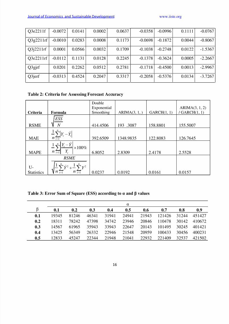
2.2. Empirical Results
Eight model selection criteria as suggested by Ramanathan (2002) were used to choosethe best forecasting models among ARIMA and GARCH models, while the best time seriesmethods for forecasting demand for petroleum products was chosen based on the values of four
criteria, namely RMSE, MAE, MAPE and U-statistics (Table 2). Finally, the selected model wasused to perform short-term forecasting for the next twelve months for demand for petroleumproducts starting from January 2013 until December 2013.

8/13/2019 Forecasting Demand for Petroleum Products in Ghana EDITED
http://slidepdf.com/reader/full/forecasting-demand-for-petroleum-products-in-ghana-edited 12/20
Journal of Economics and Sustainable Development www.iiste.org
12
The results showed that the coefficient of variation (V) of the time series data was 1.312(V>1). Because the V value was closed to 1, it was concluded that the time series data was stable(Telesca et al., 2008). The results of the regression analysis had shown that positive linear trendfactor existed in the time series data but seasonal factor was not. Referring to the AugmentedDickey-Fuller tests results, the time series data of the study was not stationary. But after the first
order of differencing was carried out, the time series data became stationary.
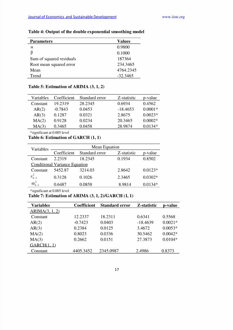
The double exponential smoothing method was used as the regression result had shownthat positive linear trend factor exists in the time series data. Double exponential smoothingmodels consisted with two parameters which were symbolized as α for the mean and β for thetrend. The best model of the double exponential smoothing was selected based on the lowestvalue of MSE (Mean Square Error) from the combination of α and β with condition 0<α, β<1.
The result showed that the combination α = 0.9 and β = 0.1 was the best forecastingmodel of double exponential smoothing method (Table 3). The double exponential smoothingmodel was written in equation form, from Table 4, as
4764.2345 *( 32.3465)T k F a bh h
All models which fulfilled the criteria of p+q≤5 have been considered and compared inthis study. There were twenty ARIMA (p, d, q) models which fulfilled the criteria(Table 5). Theparameters of the models were estimated with the least square method. Parameters which werenot significant at 5% confidence level were dropped from the model. Using the eight modelselection criteria suggested by Ramanathan (2002), the ARIMA (3, 1, 2) model was selected asthe best model among the other ARIMA models. However, the parameters of AR (1) and MA (1)were found not significant and thus dropped from the model.
Identification and estimation of GARCH (p, q) models in this study were done by
following the four steps that were ARCH effect checking, estimation, model checking andforecasting. Four GARCH (p,q) models were selected and compared, namely GARCH (1, 1),GARCH (1, 2), GARCH (2, 1) and GARCH (2, 2). Using the eight model selection criteriasuggested by Ramanathan (2002), the GARCH (1, 1) model was selected as the best modelamong the other three GARCH models(Table 6). ARCH effect which was tested by using aregression analysis existed in the ARIMA (3, 1, 2) model. What this meant was that the ARIMA(3, 1, 2) model could be mixed with the best GARCH model (i.e., GARCH(1, 1)). Four modelselection criteria were used to select the best forecasting model from the four different types of time series methods. Based on the results of the ex-post forecasting (starting from January untilDecember 2013), the ARIMA (3, 1, 2)/GARCH (1, 1) model was the best short-term forecastingmodel for the demand for petroleum products (Table 9).
A linear relationship between Q2r and GARCH family forecast for differentcombinations was also obtained. R-sq values in table of models gave the percentage of variationswhich the regression was able to explain. It was clear that relationship (7) best explains the
8/13/2019 Forecasting Demand for Petroleum Products in Ghana EDITED
http://slidepdf.com/reader/full/forecasting-demand-for-petroleum-products-in-ghana-edited 13/20
Journal of Economics and Sustainable Development www.iiste.org
13
variations in the actual returns and forecasted returns, while relationship (5) was the second bestin explaining the variations while relationship (3) was the third best in Table 8.
To determine whether there is significant difference for the mean demand and thestandard deviation values of the observed and predicted data for each month, a z-test (for means)
and F-test (for standard deviations) were applied (Haan, 1977; Devore and Peck, 1993). Sincemonthly mean values from observed and predicted data is between z-critical table values (± 1.96for 2 tailed at the 5% significance level), the data support the claim that there is no differencebetween the mean values of observed and predicted data. Similarly, monthly standard deviationvalues from observed and predicted data were smaller than F- critical table values at the 5%significance level. Furthermore, these results show that the predicted data preserve the basicstatistical properties of the observed series.
The coefficient of correlation (R), which measures the strength of the associationbetween 2 variables, and the significance level (Rsig) related to the R of regression shows thatthere is a statistically significant linear relationship between the observed and predicted data. Onthe other hand, the coefficient of determination (R-square), which is interpreted as theproportionate reduction of total variation associated with the use of the predictor variable (theobserved data in this study), and adjusted R-square measure, which presents the sample responseof the population for each regression, were close to one. In addition, the results (F-value and FSig)concerning tests applied for determining whether the estimated regression functions adequatelyfit the data emphasize that the association between the observed and predicted monthly datasequences is linear. Based on these results, it is concluded that the selected best ARIMA modelfor each station can make accurate estimates.
CONCLUSION
Seven multiple regression relationships for different combination of nested ARMA /
GARCH were used to filter their Q3 demand forecast. Filtered result analysis showsimprovements in the correlation coefficient of the forecast demands and observed Q3 demands.Correlation coefficient is positive in some simulations, which were always negative withGARCH family model’s forecast. Regression filtered results follow market trend better, whileother descriptive parameters like variance, skewness and kurtosis become more comparable toactual Q3 demand. Therefore the proposed simulation framework under given observations tosome extent has improved nested conditional mean and variance models forecast of Q3 forecastfor petroleum products under such market conditions of 2013. However, it is not generallypossible to get a definite relationship between observed and forecasted result.
This study also investigated four different types of univariate time series methods,
namely exponential smoothing, ARIMA, GARCH and the mixed ARIMA/GARCH. The resultsshowed that the mixed ARIMA/GARCH model outperformed the exponential smoothing,ARIMA and GARCH for forecasting the demand for petroleum products.
References
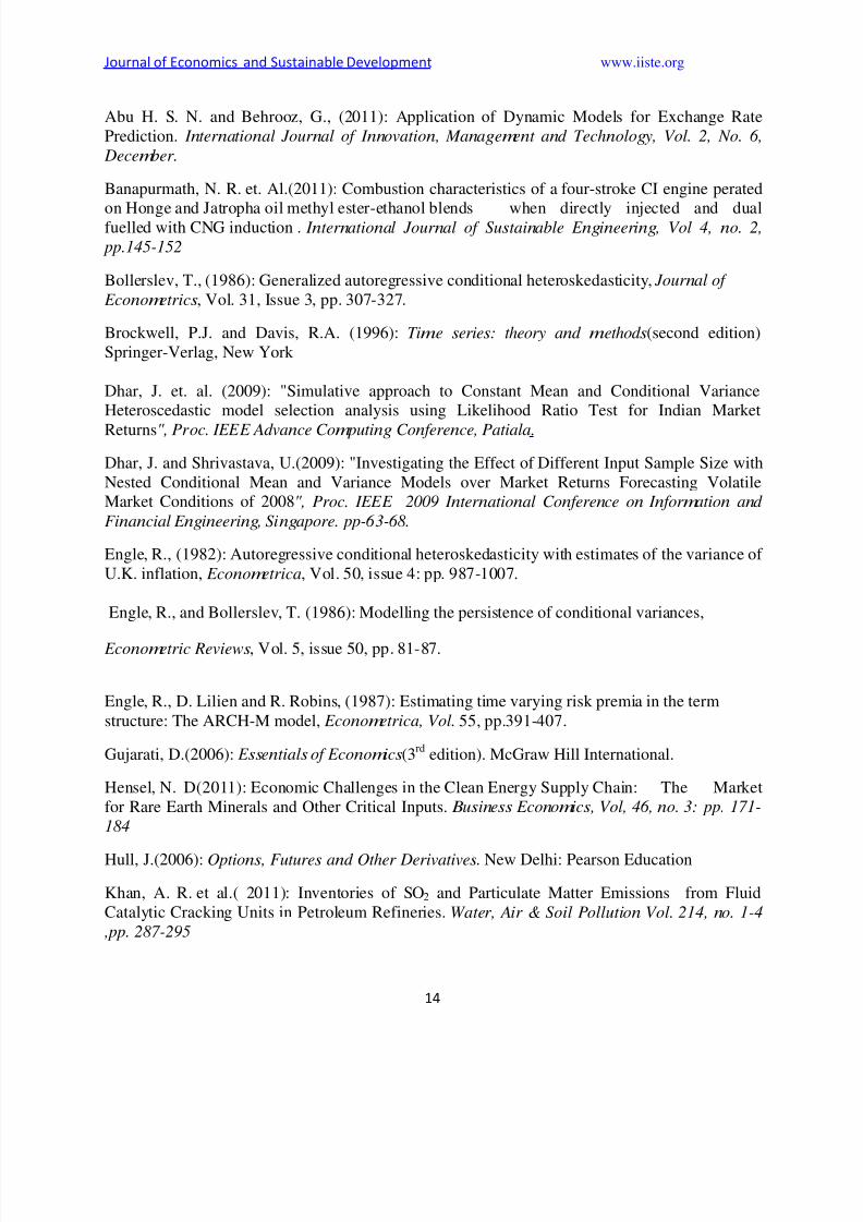
8/13/2019 Forecasting Demand for Petroleum Products in Ghana EDITED
http://slidepdf.com/reader/full/forecasting-demand-for-petroleum-products-in-ghana-edited 14/20
Journal of Economics and Sustainable Development www.iiste.org
14
Abu H. S. N. and Behrooz, G., (2011): Application of Dynamic Models for Exchange RatePrediction. International Journal of Innovation, Management and Technology, Vol. 2, No. 6,
December.
Banapurmath, N. R. et. Al.(2011): Combustion characteristics of a four-stroke CI engine perated
on Honge and Jatropha oil methyl ester-ethanol blends when directly injected and dualfuelled with CNG induction . International Journal of Sustainable Engineering, Vol 4, no. 2,
pp.145-152
Bollerslev, T., (1986): Generalized autoregressive conditional heteroskedasticity, Journal of
Econometrics, Vol. 31, Issue 3, pp. 307-327.
Brockwell, P.J. and Davis, R.A. (1996): Time series: theory and methods(second edition)Springer-Verlag, New York
Dhar, J. et. al. (2009): "Simulative approach to Constant Mean and Conditional VarianceHeteroscedastic model selection analysis using Likelihood Ratio Test for Indian Market
Returns", Proc. IEEE Advance Computing Conference, Patiala.
Dhar, J. and Shrivastava, U.(2009): "Investigating the Effect of Different Input Sample Size withNested Conditional Mean and Variance Models over Market Returns Forecasting VolatileMarket Conditions of 2008", Proc. IEEE 2009 International Conference on Information and
Financial Engineering, Singapore. pp-63-68.
Engle, R., (1982): Autoregressive conditional heteroskedasticity with estimates of the variance of U.K. inflation, Econometrica, Vol. 50, issue 4: pp. 987-1007.
Engle, R., and Bollerslev, T. (1986): Modelling the persistence of conditional variances,
Econometric Reviews, Vol. 5, issue 50, pp. 81-87.
Engle, R., D. Lilien and R. Robins, (1987): Estimating time varying risk premia in the termstructure: The ARCH-M model, Econometrica, Vol. 55, pp.391-407.
Gujarati, D.(2006): Essentials of Economics(3rd
edition). McGraw Hill International.
Hensel, N. D(2011): Economic Challenges in the Clean Energy Supply Chain: The Marketfor Rare Earth Minerals and Other Critical Inputs. Business Economics, Vol, 46, no. 3: pp. 171-
184
Hull, J.(2006): Options, Futures and Other Derivatives. New Delhi: Pearson Education
Khan, A. R. et al.( 2011): Inventories of SO2 and Particulate Matter Emissions from FluidCatalytic Cracking Units in Petroleum Refineries. Water, Air & Soil Pollution Vol. 214, no. 1-4
,pp. 287-295
8/13/2019 Forecasting Demand for Petroleum Products in Ghana EDITED
http://slidepdf.com/reader/full/forecasting-demand-for-petroleum-products-in-ghana-edited 15/20
Journal of Economics and Sustainable Development www.iiste.org
15
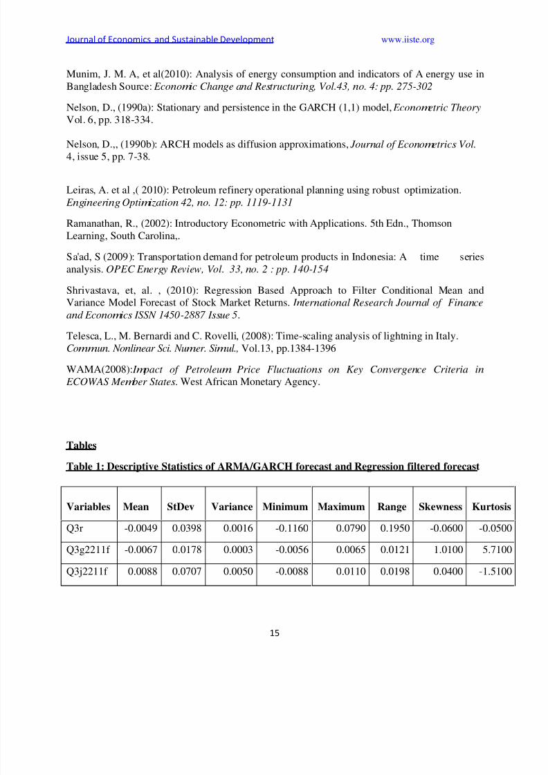
Munim, J. M. A, et al(2010): Analysis of energy consumption and indicators of A energy use inBangladesh Source: Economic Change and Restructuring, Vol.43, no. 4: pp. 275-302
Nelson, D., (1990a): Stationary and persistence in the GARCH (1,1) model, Econometric Theory
Vol. 6, pp. 318-334.
Nelson, D.,, (1990b): ARCH models as diffusion approximations, Journal of Econometrics Vol.
4, issue 5, pp. 7-38.
Leiras, A. et al ,( 2010): Petroleum refinery operational planning using robust optimization. Engineering Optimization 42, no. 12: pp. 1119-1131
Ramanathan, R., (2002): Introductory Econometric with Applications. 5th Edn., ThomsonLearning, South Carolina,.
Sa'ad, S (2009): Transportation demand for petroleum products in Indonesia: A time series
analysis. OPEC Energy Review, Vol. 33, no. 2 : pp. 140-154
Shrivastava, et, al. , (2010): Regression Based Approach to Filter Conditional Mean andVariance Model Forecast of Stock Market Returns. International Research Journal of Finance
and Economics ISSN 1450-2887 Issue 5.
Telesca, L., M. Bernardi and C. Rovelli, (2008): Time-scaling analysis of lightning in Italy.Commun. Nonlinear Sci. Numer. Simul., Vol.13, pp.1384-1396
WAMA(2008): Impact of Petroleum Price Fluctuations on Key Convergence Criteria in
ECOWAS Member States. West African Monetary Agency.
Tables
Table 1: Descriptive Statistics of ARMA/GARCH forecast and Regression filtered forecast
Variables Mean StDev Variance Minimum Maximum Range Skewness Kurtosis
Q3r -0.0049 0.0398 0.0016 -0.1160 0.0790 0.1950 -0.0600 -0.0500
Q3g2211f -0.0067 0.0178 0.0003 -0.0056 0.0065 0.0121 1.0100 5.7100
Q3j2211f 0.0088 0.0707 0.0050 -0.0088 0.0110 0.0198 0.0400 -1.5100
8/13/2019 Forecasting Demand for Petroleum Products in Ghana EDITED
http://slidepdf.com/reader/full/forecasting-demand-for-petroleum-products-in-ghana-edited 16/20
Journal of Economics and Sustainable Development www.iiste.org
16
Table 2: Criteria for Assessing Forecast Accuracy
Criteria Formula
DoubleExponential
Smoothing ARIMA(3, 1, ) GARCH(1, 1)
ARIMA(3, 1, 2)
/ GARCH(1, 1)
RSME
ESS
N 414.4506 193 .3087 158.8801 155.5007
MAE 1
1 n
t t
t
Y Y n
392.6509 1348.9835 122.8083 126.7645
MAPE 1
1100%
nt t
t t
Y Y
n Y
6.8052 2.8309 2.4178 2.5528
U-Statistics
2 2
1 1
1 1n n
t t
RSME
Y Y n n
0.0237 0.0192 0.0161 0.0157
Table 3: Error Sum of Square (ESS) according to α and β values
βα
0.1 0.2 0.3 0.4 0.5 0.6 0.7 0.8 0.9
0.1 19345 81246 46341 31941 24941 21943 121426 31244 451427
0.2 18311 78242 47398 34742 23946 20846 110478 30142 410672
0.3 14567 61965 35943 33943 22647 20143 101495 30245 4014210.4 13425 56349 26332 22946 21548 20959 100433 30456 400231
0.5 12833 45247 22344 21948 21041 22932 221409 32537 421502
Q3e2211f -0.0072 0.0141 0.0002 0.0637 -0.0358 -0.0996 0.1111 -0.0767
Q3g2211rf -0.0010 0.0283 0.0008 0.1173 -0.0698 -0.1872 0.0044 -0.8067
Q3j2211rf 0.0001 0.0566 0.0032 0.1709 -0.1038 -0.2748 0.0122 -1.5367
Q3e2211rf -0.0112 0.1131 0.0128 0.2245 -0.1378 -0.3624 0.0005 -2.2667
Q3gjrf 0.0201 0.2262 0.0512 0.2781 -0.1718 -0.4500 0.0013 -2.9967
Q3jerf -0.0313 0.4524 0.2047 0.3317 -0.2058 -0.5376 0.0134 -3.7267
8/13/2019 Forecasting Demand for Petroleum Products in Ghana EDITED
http://slidepdf.com/reader/full/forecasting-demand-for-petroleum-products-in-ghana-edited 17/20
Journal of Economics and Sustainable Development www.iiste.org
17
Table 4: Output of the double exponential smoothing model
Parameters Values
α 0.9800β 0.1000
Sum of squared residuals 187364Root mean squared error 234.3465
Mean 4764.2345
Trend -32.3465
Table 5: Estimation of ARIMA (3, 1, 2)
Variables Coefficient Standard error Z-statistic p-value
Constant 19.2319 28.2345 0.6934 0.4562
AR(2) -0.7843 0.0453 -18.4653 0.0001*
AR(3) 0.1287 0.0321 2.8675 0.0023*MA(2) 0.9128 0.0234 20.3465 0.0002*
MA(3) 0.3465 0.0458 28.9874 0.0134*
*significant at 0.005 level
Table 6: Estimation of GARCH (1, 1)
VariablesMean Equation
Coefficient Standard error Z-statistic p-value
Constant 2.2319 18.2345 0.1934 0.8502
Conditional Variance Equation
Constant 5452.87 3214.03 2.8642 0.0123*2
1εk 0.3128 0.1026 2.3465 0.0302*2
1k σ 0.6487 0.0858 8.9814 0.0134*
*significant at 0.005 level
Table 7: Estimation of ARIMA (3, 1, 2)/GARCH (1, 1)
Variables Coefficient Standard error Z-statistic p-value
ARIMA(3, 1, 2)
Constant 12.2337 18.2311 0.6341 0.5568
AR(2) -0.7423 0.0403 -18.4639 0.0021*
AR(3) 0.2384 0.0125 3.4672 0.0053*
MA(2) 0.8023 0.0336 30.5462 0.0042*
MA(3) 0.2662 0.0151 27.3873 0.0104*
GARCH(1, 1)
Constant 4405.3452 2345.0987 2.4986 0.8373
8/13/2019 Forecasting Demand for Petroleum Products in Ghana EDITED
http://slidepdf.com/reader/full/forecasting-demand-for-petroleum-products-in-ghana-edited 18/20
Journal of Economics and Sustainable Development www.iiste.org
18
2
1εk 0.3254 0.0975 2.4863 0.0034*2
1k σ 0.7654 0.1203 7.9073 0.0002*
*significant at 0.005 level
Figure 1: AFC and PACF Plots
Table 10: Regression Statistics with Q2r on LHS and Q2g2211f, Q2e2211f on RHS
RelationshipRegression
order K Q2g2211f Q2j2211f Q2e2211f p-value R-Sq
R-Sq(adj.)
1 1 -0.001 0.07 0 0 0.0264 0% 0%
2 1 0.007 0 3.23 0 0.0262 1.50% 0%
3 1 0.010 0 0 3.01 0.0257 4.90% 3.40%
4 2 0.008 0.45 3.41 0 0.0263 1.60% 0%
5 2 0.003 0 -17.6 0 0.0251 10.60% 7.70%
6 2 0.010 0.34 3.04 2.06 0.0259 5.0% 1.80%
7 3 0.008 -0.89 -17.7 11.3 0.0349 11.20% 7.60%
8/13/2019 Forecasting Demand for Petroleum Products in Ghana EDITED
http://slidepdf.com/reader/full/forecasting-demand-for-petroleum-products-in-ghana-edited 19/20
Journal of Economics and Sustainable Development www.iiste.org
19
Figure 2: Time Series Plots of Residuals
8/13/2019 Forecasting Demand for Petroleum Products in Ghana EDITED
http://slidepdf.com/reader/full/forecasting-demand-for-petroleum-products-in-ghana-edited 20/20
Journal of Economics and Sustainable Development www.iiste.org
20
.