Forecasting Environmental and Social Externalities ... · OCS Study BOEM 2015-053 Forecasting Environmental and Social Externalities Associated with Outer Continental Shelf (OCS)

OCS Study BOEM 2015-053

Forecasting Environmental and Social Externalities Associated with Outer Continental Shelf (OCS) Oil and Gas Development – Volume 2: Supplemental Information to the 2015 Revised Offshore Environmental Cost Model (OECM)

US Department of the Interior Bureau of Ocean Energy Management Headquarters December 2015

[This page intentionally left blank.]

OCS Study BOEM 2015-053

Forecasting Environmental and Social Externalities Associated with Outer Continental Shelf (OCS) Oil and Gas Development – Volume 2: Supplemental Information to the 2015 Revised Offshore Environmental Cost Model (OECM) Prepared by

Industrial Economics, Incorporated 2067 Massachusetts Avenue Cambridge, MA 02140 and SC&A, Incorporated

1608 Spring Hill Road, Suite 400

Vienna, VA 22182

US Department of the Interior Bureau of Ocean Energy Management Headquarters

December 2015

DISCLAIMER

Study concept, oversight, and funding were provided by the US Department of the Interior, Bureau of

Ocean Energy Management, Environmental Studies Program, Washington, DC, under Contract Number

GS-10F-0093K, order number M14PD00057. This report has been technically reviewed by BOEM and it

has been approved for publication. The views and conclusions contained in this document are those of the

authors and should not be interpreted as representing the opinions or policies of the US Government, nor

does mention of trade names or commercial products constitute endorsement or recommendation for use.

REPORT AVAILABILITY

To download a PDF file of this Environmental Studies Program report, go to the US Department of the

Interior, Bureau of Ocean Energy Management, Environmental Studies Program Information System

website and search on OCS Study BOEM 2015-053.

CITATION

Industrial Economics, Inc. and SC&A, Inc. 2015. Forecasting Environmental and Social Externalities

Associated with Outer Continental Shelf (OCS) Oil and Gas Development - Volume 2:

Supplemental Information to the 2015 Revised OECM. U.S. Department of the Interior, Bureau

of Ocean Energy Management. OCS Study BOEM 2015-053.

http://www.boem.gov/Environmental-Stewardship/Environmental-Studies-Program-Information-System.aspx

i

Contents

List of Figures ................................................................................................................................ iii

List of Tables ................................................................................................................................ iv

Abbreviations and Acronyms ........................................................................................................ vi

1. Introduction ..........................................................................................................................1

2. Energy Alternatives and the Environment ...........................................................................3

2.1 Overview of Energy Services ..................................................................................3

2.1.1 Oil and Gas Uses and Alternatives: Residential Sector ...............................6

2.1.2 Oil and Gas Uses and Alternatives: Commercial Sector .............................8

2.1.3 Oil and Gas Uses and Alternatives: Industrial Sector ..................................9

2.1.4 Oil and Gas Uses and Alternatives: Transportation Sector .......................10

2.1.5 Oil and Gas Uses and Alternatives: Electricity ..........................................10

2.2 Current and Future Production of Energy Sources ................................................11

2.2.1 Current and Future Energy Use .................................................................11

2.2.2 Renewable Energy Current and Future Use ...............................................12

2.2.3 Nuclear Energy Current and Future Use ....................................................23

2.2.4 Other Natural Gas Current and Future Use................................................24

2.2.5 Location of Solar Energy Facilities/Opportunities in the United States ....24

2.2.6 Location of wind Energy Facilities in the United States ...........................26

2.3 Environmental and Social Costs of Energy Sources ..............................................27

2.3.1 Overview of Environmental and Social Costs of Energy Sources ............27

2.3.2 Waste Management ....................................................................................28

2.3.3 Mining Health and Safety ..........................................................................29

2.3.4 Groundwater Impacts .................................................................................29

2.3.5 Surface Water Impacts ...............................................................................29

2.3.6 Air Quality Impacts ....................................................................................30

2.3.7 Socioeconomic Impacts .............................................................................31

2.3.8 Ecological and Wildlife Impacts ................................................................31

2.3.9 Onshore Spills ............................................................................................31

2.3.10 Environmental and Social Impacts by Energy Source ...............................32

2.4 References ..............................................................................................................58

3. Analysis of Impacts from Catastrophic Oil Spills .............................................................64

3.1 Response Costs ......................................................................................................65

3.1.1 Variability and Uncertainty of Response Costs .........................................65

3.1.2 Estimation of Response Costs by Region ..................................................66

3.2 Ecological Damages ...............................................................................................68

3.2.1 Gulf of Mexico ...........................................................................................69

3.2.2 Atlantic .......................................................................................................70

3.2.3 Cook Inlet...................................................................................................72

3.2.4 Arctic..........................................................................................................72

3.2.5 Summary ....................................................................................................73

3.3 Recreational Use ....................................................................................................73

ii

3.3.1 Shoreline Recreation and Boating .............................................................75

3.3.2 Wildlife Viewing .......................................................................................86

3.4 Commercial Fishing ...............................................................................................87

3.4.1 Commercial Fishing Approach ..................................................................88

3.5 Subsistence .............................................................................................................91

3.5.1 Cook Inlet...................................................................................................92

3.5.2 Arctic..........................................................................................................93

3.6 Fatal and Nonfatal Injuries .....................................................................................95

3.7 Value of Spilled Oil Not Recovered ......................................................................95

3.8 Impacts of Dispersants and In-Situ Burns .............................................................96

3.9 Uncertainties ..........................................................................................................96

3.10 References ............................................................................................................101

Appendix A: Damage Estimates for Additional CDE Scenarios in the Atlantic Region ..........108

Shoreline Recreation ........................................................................................................108

Inland Fishing ..................................................................................................................110

Commercial Fishing .........................................................................................................111

Uncertainty .......................................................................................................................112

Appendix B. Supplemental Recreational Use Values For The Gulf Of Mexico .......................113

iii

List of Figures

Figure 1. Primary energy consumption by fuel in the reference case, 1980–2040 (quadrillion

Btu) ................................................................................................................................12

Figure 2. Renewable electricity by fuel type in the Reference case, 2000–2040 (billion

kilowatt hours) ...................................................................................................................13

Figure 3. Electricity generation by type of biomass energy source ..............................................14

Table 8. Renewable generation amount and percentage of total energy produced ......................14

Table 9. Comparison of baseline, reference case, and REmap analysis energy supply and

demand ...............................................................................................................................16

Figure 4. Geographic market potential for biodiesel ....................................................................17

Figure 5. Geographic market potential for ethanol .......................................................................19

Figure 6. Geographic market potential for biomass energy ..........................................................20

Figure 7. Geographic market potential for geothermal energy .....................................................21

Figure 8. Top non-powered dams with hydroelectric energy potential ........................................22

Figure 9. Operational landfill gas projects and candidate landfills for future landfill gas

projects by state..................................................................................................................23

Figure 10. Geographic market potential for biomass gas .............................................................24

Figure 11. Geographic market potential for concentrating solar resources ..................................25

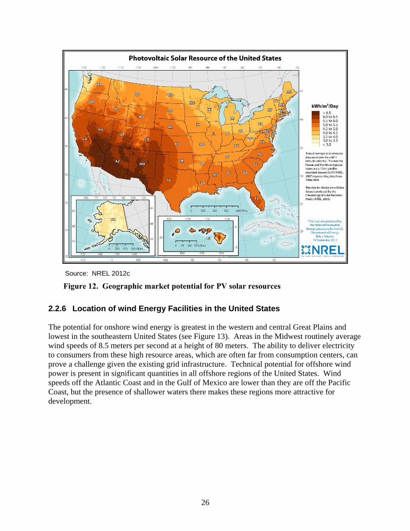
Figure 12. Geographic market potential for PV solar resources ...................................................26

Figure 13. Geographic market potential for wind energy .............................................................27

Figure 14. Map of recreation sites sampled in the Deepwater Horizon lost recreational use

assessment ..........................................................................................................................77

iv

List of Tables

Table 1. 2013 residential energy end-use splits, by fuel type (quadrillion Btu) .............................7

Table 2. AEO2015 residential energy source projections ..............................................................7

Table 3. 2013 commercial energy end-use splits, by fuel type (quadrillion Btu) ...........................8

Table 4. AEO2015 commercial energy source projections ............................................................9

Table 5. AEO2015 industrial sector energy source projections .....................................................9

Table 6. AEO2015 transportation sector energy source projections ............................................10

Table 7. AEO2015 electricity fuel projections .............................................................................11

Table 8. Renewable generation amount and percentage of total energy produced ......................14


demand ...............................................................................................................................16

Table 10. Onshore oil and gas production ....................................................................................33

Table 11. Oil and gas imports .......................................................................................................35

Table 12. Coal production.............................................................................................................36

Table 13. Biofuels .........................................................................................................................39

Table 14. Biomass .........................................................................................................................41

Table 15. Geothermal....................................................................................................................43

Table 16. Hydroelectric ................................................................................................................45

Table 17. Municipal waste ............................................................................................................47

Table 18. Nuclear ..........................................................................................................................49

Table 19. Other natural gas ...........................................................................................................51

Table 20. Other oil ........................................................................................................................52

Table 21. Solar ..............................................................................................................................54

Table 22. Wind (onshore and offshore) ........................................................................................56

Table 23. Distribution of shoreline habitat ...................................................................................67

Table 24. Estimated response costs per barrel by geographic region ...........................................68

Table 25. NRDA estimates of ecological damages from past spills on the Gulf Coast

(2017$) ...............................................................................................................................70

Table 26. NRDA estimates of ecological damages from past spills on the Atlantic Coast

(2017$) ...............................................................................................................................71

Table 27. Range of NRDA costs by geographic region (2017$) ..................................................73

Table 28. Duration of losses to shoreline recreation, by region and activity, for the

Deepwater Horizon lost recreational use assessment ........................................................77

v

Table 29. Deepwater Horizon shoreline and inland fishing study lost use estimates – tier 1 ......78

Table 30. Deepwater Horizon boating study lost use estimates - tier 1 ........................................78

Table 31. Summary of Tier 1 recreation impacts associated with the Deepwater Horizon

spill 79

Table 32. Tier 2 secondary shoreline study damages ....................................................................80

Table 33. Summary of recreational impacts associated with the Deepwater Horizon oil spill ....80

Table 34. Beach use baseline for the Atlantic ...............................................................................82

Table 35. Recreational inland angler trips baseline for the Atlantic : May – March impact

period 83

Table 36. Estimated reduction in recreational activitity in the Atlantic following a CDE ...........84

Table 37. Summary of recreational damages associated with a CDE in the Atlantic ...................84

Table 38. Estimated change in Gulf of Mexico landings volume following the Deepwater

Horizon oil spill .................................................................................................................89

Table 39. Estimated change in Gulf of Mexico landings revenue following the Deepwater

Horizon oil spill .................................................................................................................89

Table 40. Commercial fishery landings revenue in the mid-Atlantic (2017$) .............................91

Table 41. Average annual Cook Inlet commercial fishery landings (2017$) ...............................91

Table 42. Estimated Cook Inlet subsistence losses .......................................................................93

Table 43. Estimated Arctic subsistence losses ..............................................................................94

Table 44. Uncertainties, limitations, and assumptions of analysis ...............................................97

Table A-1. Baseline shoreline use for alternative scenarios: may of spill year through

November of the following year ......................................................................................109

Table A-2. Shoreline use damages summary for alternative scenarios ......................................110

Table A-3. inland fishing baseline for alternative scenarios: May of spill year through

March the following year .................................................................................................110

Table A-4. Inland fishing damages for alternative scenarios .....................................................111

Table A-5. Commercial fishing baseline and damages for alternative scenarios (2017$) .........112

Table B-1. Gulf of Mexico valuation studies for beach recreation .............................................113

Table B-2. GOM recreational fisher per trip valuation estimates ...............................................113

vi

Abbreviations and Acronyms

AEO2013 Annual Energy Outlook 2013

AEO2015 Annual Energy Outlook 2015

ARC Appalachian Regional Commission

BOEM Bureau of Ocean Energy Management

Btu British thermal unit (equal to about 1055 joules)

CAFE corporate average fuel economy

CDEs catastrophic discharge events

CO carbon monoxide

CSR Concentrating Solar Resources

DOE U.S. Department of Energy

DOI U.S. Department of the Interior

DOL U.S. Department of Labor

DPP Draft Proposed Program

DWH Deepwater Horizon

E&D exploration and development

EDWPC East Delhi Waste Processing Company Pvt. Ltd.

EGS Enhanced Geothermal System

EIA U.S. Energy Information Administration

EPA US Environmental Protection Agency

FAO Food and Agriculture Organization of the United Nations

FFV flexible-fuel vehicle

FWS U.S. Fish and Wildlife Service

GAO Government Accountability Office

GLC Great Lakes Commission

gW gigawatt

GWh gigawatt hour

IRENA International Renewable Energy Agency

kWh/m2 kilowatt hour per square meter

LCF latent cancer fatality

LFG landfill gas

LMOP Landfill Methane Outreach Program

LPG liquefied petroleum gas

m meter(s)

MarketSim Market Simulation Model

mmscfd Million Standard Cubic Feet per Day (gas distribution)

MMTCO2e/yr million metric tons of carbon dioxide equivalent per year

MRIP Marine Recreational Information Program

MSW municipal solid waste

MW megawatt

NMFS National Marine Fisheries Service

NOAA National Oceanic and Atmospheric Administration

NOx nitrogen oxides

NRC U.S. Nuclear Regulatory Commission

NRDA natural resource damage assessment

vii

NRDC Natural Resources Defense Council

NREL National Renewable Energy Laboratory

NSRE 2000 National Survey of Recreation in the Environment

NYT New York Times

OCS Outer Continental Shelf

OECM Offshore Environmental Cost Model

ORNL Oak Ridge National Laboratory

OSIR Oil Spill Intelligence Report

PBS Public Broadcasting System

PDARP Preliminary Damage Assessment and Restoration Plan

PJ petajoule

PM particulate matter

PV photovoltaic

PVC photovoltaic cell

RDF refuse-derived fuel

RUM Randomized Utility Maximization

SNG synthetic natural gas

SO2 sulfur dioxide

TEEIC Tribal Energy and Environmental Information Clearinghouse

TNC The Nature Conservancy

Trustees Deepwater Horizon Oil Spill Natural Resource Trustees

TVA Tennessee Valley Authority

TWh terawatt hours

USDA U.S. Department of Agriculture

USGS United States Geological Survey

UTTR undiscovered technically recoverable resources

VOC volatile organic compound

VSL value of a statistical life

WTG wind turbine generator

WTP willingness to pay

1

1. Introduction

The Bureau of Ocean Energy Management (BOEM) is charged with assisting the U.S. Secretary

of the Interior in carrying out the mandates of the Outer Continental Shelf (OCS) Lands Act

(Act), which calls for expedited exploration and development (E&D) of the OCS to, among other

goals, “reduce dependence on foreign sources and maintain a favorable balance of payments in

world trade.” The Act also requires that BOEM prepare forward-looking five year schedules of

proposed OCS lease sales that define as specifically as possible the size, timing, and location of

the OCS territory(ies) to be offered for lease. As part of the development of these “Five Year

Programs,” BOEM completes an analysis of the environmental and social costs attributable to

the exploration, development, production, and transport of oil and natural gas anticipated to

result from the Program proposal, net of the environmental and social costs attributable to the No

Action Alternative (NAA) (i.e., the costs associated with energy production from sources that

would substitute for OCS production in the absence of the Program) and net of any benefits

(measured as “negative costs”) attributable to OCS oil- and natural gas-related activities.

To estimate the anticipated environmental and social costs attributable to oil and natural gas

E&D activities on the OCS, as specified in an E&D scenario,1 BOEM utilizes the Offshore

Environmental Cost Model (OECM), a revised Microsoft (MS) Access-based model, which has

been updated in conjunction with development of the 2017-2022 Program. The OECM was

designed to focus on capturing the most significant environmental and social costs from the

proposed action and NAA. The report Forecasting Environmental and Social Externalaties

Associated with the Outer Continental Shelf (OCS) Oil and Gas Development – Volume 1: The

2015 Revised Offshore Environmental Cost Model (OECM) (BOEM 2015-052) presents the

model’s cost calculation methodologies as well as descriptions of each calculation driver,

including the sources of underlying data and any necessary assumptions. The purpose of this

companion report (Volume 2) is to present supplemental information on environmeantal and

social costs that BOEM considers in conjunction with the OECM results.

The OECM was designed to focus on the “main” energy market substitutions (i.e. increased

imports and onshore production of oil and natural gas, fuel switching to coal, and reduced

demand likely to occur as a direct result of programmatic decisions to make OCS oil and gas

resources unavailable to the market) but multiple other “minor” energy substitutes (those that

might occur in small quantities or without regard to programmatic decisions) exist. Chapter 2 of

this report, Energy Alternatives and the Environment, gives consideration of the full range of

possible energy sources sources that may potentially replace OCS production (including those

not directly evaluated in the OECM) and provides a qualitative discussion of their environmental

and social costs, recognizing that all energy sources have externalities. Specifically, the chapter

presents oil and gas uses and alternatives by sector (e.g. residential, commercial, industrial,

transportation, and electricity) and discusses current and future production trends and the

environmental and social costs of the different energy sources.

1 An E&D scenario defines the incremental level of OCS exploration, development, and production activity

anticipated to occur within planning areas expected to be made available for leasing in the BOEM Five Year OCS Oil and Gas Leasing Program. Elements of an E&D scenario include the number of exploration wells drilled, the number of platforms installed, the number of development wells drilled, miles of new pipeline constructed, anticipated aggregate oil and gas production, and the number of platforms removed.

2

While many of the impacts that the OECM estimates are associated with the possibility of oil

spills from pipelines, tankers, and OCS platforms, it does not include impacts from catastrophic

discharge events (CDEs) because these are extremely unlikely and their potential impacts

difficult to estimate due to large variability in the factors that contribute to impacts. To

supplement the costs considered in the OECM, Chapter 3 of this report, Analysis of Impacts from

a Catastrophic Spill provides information on the potential environmental and social costs of a

CDE. This chapter provides an overview of the available data and literature on potential CDE

impacts, including response costs, ecological impacts, recreational impacts, commercial fishing

impacts, fatal and nonfatal injuries, and value of oil spilled.

3

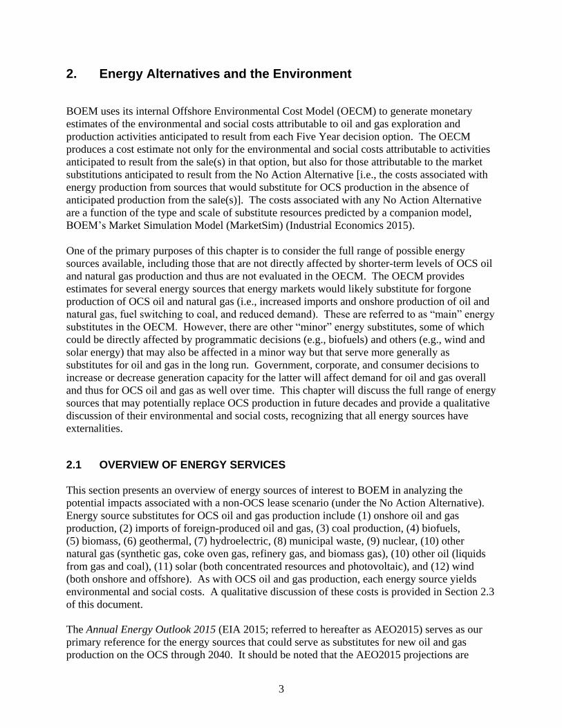
2. Energy Alternatives and the Environment

BOEM uses its internal Offshore Environmental Cost Model (OECM) to generate monetary

estimates of the environmental and social costs attributable to oil and gas exploration and

production activities anticipated to result from each Five Year decision option. The OECM

produces a cost estimate not only for the environmental and social costs attributable to activities

anticipated to result from the sale(s) in that option, but also for those attributable to the market

substitutions anticipated to result from the No Action Alternative [i.e., the costs associated with

energy production from sources that would substitute for OCS production in the absence of

anticipated production from the sale(s)]. The costs associated with any No Action Alternative

are a function of the type and scale of substitute resources predicted by a companion model,

BOEM’s Market Simulation Model (MarketSim) (Industrial Economics 2015).

One of the primary purposes of this chapter is to consider the full range of possible energy

sources available, including those that are not directly affected by shorter-term levels of OCS oil

and natural gas production and thus are not evaluated in the OECM. The OECM provides

estimates for several energy sources that energy markets would likely substitute for forgone

production of OCS oil and natural gas (i.e., increased imports and onshore production of oil and

natural gas, fuel switching to coal, and reduced demand). These are referred to as “main” energy

substitutes in the OECM. However, there are other “minor” energy substitutes, some of which

could be directly affected by programmatic decisions (e.g., biofuels) and others (e.g., wind and

solar energy) that may also be affected in a minor way but that serve more generally as

substitutes for oil and gas in the long run. Government, corporate, and consumer decisions to

increase or decrease generation capacity for the latter will affect demand for oil and gas overall

and thus for OCS oil and gas as well over time. This chapter will discuss the full range of energy

sources that may potentially replace OCS production in future decades and provide a qualitative

discussion of their environmental and social costs, recognizing that all energy sources have

externalities.

2.1 OVERVIEW OF ENERGY SERVICES

This section presents an overview of energy sources of interest to BOEM in analyzing the

potential impacts associated with a non-OCS lease scenario (under the No Action Alternative).

Energy source substitutes for OCS oil and gas production include (1) onshore oil and gas

production, (2) imports of foreign-produced oil and gas, (3) coal production, (4) biofuels,

(5) biomass, (6) geothermal, (7) hydroelectric, (8) municipal waste, (9) nuclear, (10) other

natural gas (synthetic gas, coke oven gas, refinery gas, and biomass gas), (10) other oil (liquids

from gas and coal), (11) solar (both concentrated resources and photovoltaic), and (12) wind

(both onshore and offshore). As with OCS oil and gas production, each energy source yields

environmental and social costs. A qualitative discussion of these costs is provided in Section 2.3

of this document.

The Annual Energy Outlook 2015 (EIA 2015; referred to hereafter as AEO2015) serves as our

primary reference for the energy sources that could serve as substitutes for new oil and gas

production on the OCS through 2040. It should be noted that the AEO2015 projections are

4

based generally on federal, state, and local laws and regulations in effect as of the end of October

2014. The potential impacts of pending or proposed legislation, regulations, and standards are

not reflected in the projections [for example, the U.S. Environmental Protection Agency’s

(EPA’s) proposed Clean Power Plan]. In certain situations, however, where it is clear that a law

or a regulation will take effect shortly after the publication of AEO2015, it may be considered in

the projection.

U.S. energy consumption is expected to grow at a modest rate over the AEO2015 projection

period, averaging 0.3% per year from 2013 through 2040 in the Reference case. A marginal

decrease in energy consumption in the transportation sector contrasts with growth in most other

sectors. Declines in energy consumption tend to result from the adoption of more energy-

efficient technologies and existing policies that promote increased energy efficiency.

The following briefly defines each energy source.

Onshore Oil and Gas Production is crude oil and natural gas supplied from resources in the

lower 48 states. Crude oil supply includes lease condensate, and natural gas is differentiated

between non-associated gas and associated-dissolved gas. Non-associated natural gas is gas in a

reservoir that is not in contact with significant quantities of crude oil. Associated-dissolved

natural gas consists of the combined volume of natural gas that occurs in crude oil reservoirs

either as free gas (associated) or as gas in solution with crude oil (dissolved).

Foreign Oil and Gas Imports represent crude oil and natural gas imported into the United States

from foreign countries.

Fuel Switching to Coal reflects increases in coal production to replace OCS oil and gas

production. It is important to note that coal is only a viable substitute for oil and gas for some

end-use sectors (e.g., electricity generation).

Biofuels are liquid fuels and blending components produced from biomass (plant) feedstocks and

are primarily used as energy for the transportation sector. Biodiesel, which is typically made

from soybean, canola, or other vegetable oils; animal fats; or recycled grease, is a biofuel that

can serve as a substitute for petroleum-derived diesel fuel or distillate fuel oil. Ethanol is a

biofuel that is used principally for blending in low concentrations with motor gasoline as an

oxygenate or octane enhancer. In high concentrations, ethanol is used to fuel alternative-fuel

vehicles specially designed for its use.

Biomass is an organic non-fossil material of biological origin that constitutes a renewable energy

source. Two major examples of biomass are wood/wood-derived fuels and biomass waste.

Wood and products derived from wood that are used as fuel include round wood (cord wood),

limb wood, wood chips, bark, sawdust, forest residues, charcoal, paper pellets, railroad ties,

utility poles, black liquor, red liquor, sludge wood, spent sulfite liquor, and other wood-based

solids and liquids. Biomass waste is organic non-fossil material of biological origin that is a

byproduct or a discarded product (e.g., agricultural crop byproducts).

5

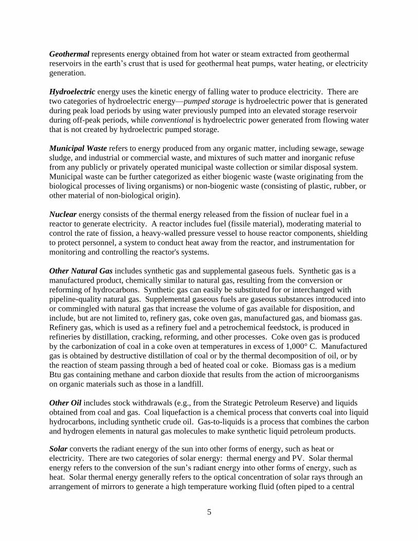
Geothermal represents energy obtained from hot water or steam extracted from geothermal

reservoirs in the earth’s crust that is used for geothermal heat pumps, water heating, or electricity

generation.

Hydroelectric energy uses the kinetic energy of falling water to produce electricity. There are

two categories of hydroelectric energy—pumped storage is hydroelectric power that is generated

during peak load periods by using water previously pumped into an elevated storage reservoir

during off-peak periods, while conventional is hydroelectric power generated from flowing water

that is not created by hydroelectric pumped storage.

Municipal Waste refers to energy produced from any organic matter, including sewage, sewage

sludge, and industrial or commercial waste, and mixtures of such matter and inorganic refuse

from any publicly or privately operated municipal waste collection or similar disposal system.

Municipal waste can be further categorized as either biogenic waste (waste originating from the

biological processes of living organisms) or non-biogenic waste (consisting of plastic, rubber, or

other material of non-biological origin).

Nuclear energy consists of the thermal energy released from the fission of nuclear fuel in a

reactor to generate electricity. A reactor includes fuel (fissile material), moderating material to

control the rate of fission, a heavy-walled pressure vessel to house reactor components, shielding

to protect personnel, a system to conduct heat away from the reactor, and instrumentation for

monitoring and controlling the reactor's systems.

Other Natural Gas includes synthetic gas and supplemental gaseous fuels. Synthetic gas is a

manufactured product, chemically similar to natural gas, resulting from the conversion or

reforming of hydrocarbons. Synthetic gas can easily be substituted for or interchanged with

pipeline-quality natural gas. Supplemental gaseous fuels are gaseous substances introduced into

or commingled with natural gas that increase the volume of gas available for disposition, and

include, but are not limited to, refinery gas, coke oven gas, manufactured gas, and biomass gas.

Refinery gas, which is used as a refinery fuel and a petrochemical feedstock, is produced in

refineries by distillation, cracking, reforming, and other processes. Coke oven gas is produced

by the carbonization of coal in a coke oven at temperatures in excess of 1,000° C. Manufactured

gas is obtained by destructive distillation of coal or by the thermal decomposition of oil, or by

the reaction of steam passing through a bed of heated coal or coke. Biomass gas is a medium

Btu gas containing methane and carbon dioxide that results from the action of microorganisms

on organic materials such as those in a landfill.

Other Oil includes stock withdrawals (e.g., from the Strategic Petroleum Reserve) and liquids

obtained from coal and gas. Coal liquefaction is a chemical process that converts coal into liquid

hydrocarbons, including synthetic crude oil. Gas-to-liquids is a process that combines the carbon

and hydrogen elements in natural gas molecules to make synthetic liquid petroleum products.

Solar converts the radiant energy of the sun into other forms of energy, such as heat or

electricity. There are two categories of solar energy: thermal energy and PV. Solar thermal

energy refers to the conversion of the sun’s radiant energy into other forms of energy, such as

heat. Solar thermal energy generally refers to the optical concentration of solar rays through an

arrangement of mirrors to generate a high temperature working fluid (often piped to a central

6

engine). Photovoltaic (PV) solar energy uses a photovoltaic cell (PVC) to convert sunlight into

electricity (direct current). A PVC is an electronic device consisting of layers of semiconductor

materials fabricated to form a junction (adjacent layers of materials with different electronic

characteristics) and electrical contacts.

Wind energy is kinetic energy present in wind motion that can be converted to mechanical

energy for driving pumps, mills, and electric power generators.

The following sections are organized by sector (residential, commercial, industrial, and

transportation) and include an evaluation of the data drawn from AEO2015 as they relate to

energy use in each sector. The primary energy sources included in this discussion are coal,

electricity, natural gas, petroleum, and renewables. The discussion by sector is followed by a

section on the energy sources responsible for electricity generation, which include coal, natural

gas, nuclear, renewables, and petroleum.

2.1.1 Oil and Gas Uses and Alternatives: Residential Sector

Table 1 presents data on the use of energy in the residential sector. Natural gas is predominantly

used for space and water heating, cooking, and wet cleaning. Fuel oil, which is not used much in

this sector, is primarily used for space and water heating.

Alternatives to these uses of natural gas and oil include liquefied petroleum gas (LPG),

renewables (used directly), and electricity. Energy use in this sector is expected to decline in

part because many homeowners are implementing efficiency upgrades to decrease the demand

for space heating, which can be viewed as a substitute for the use of oil and gas. These

efficiency upgrades refer to efficiency improvements in the construction of buildings to retain

heat, rather than the efficiency of the heating equipment itself. Measures such as adding

insulation, sealing leaks, and installing more efficient windows reduce the energy required to

maintain a desired temperature. It is also expected that over the long term consumers will

replace oil- and gas-fired equipment and appliances with electric-powered units, which are

readily available, widely used, and have a lower capital cost.

7

Table 1. 2013 residential energy end-use splits, by fuel type (quadrillion Btu)

Natural Gas Fuel Oil LPG Other Fuel (1) Renewable Energy (2) Electric (3)

Space Heating (4) 3.32 0.44 0.30 0.01 0.58 1.63

Water Heating 1.20 0.05 0.06

1.35

Cooking 0.21 0.03 0.3

Wet Cleaning (7) 0.05 0.98

Space Cooling 0.02 2.03

Other (8) 0.25 0.01 0.04

3.66

Lighting 1.81

Refrigeration (5) 1.35

Electronics (6) 1.01

Computers 0.37

Total 5.05 0.50 0.43 0.01 0.58 14.54

Notes: (1) Kerosene assumed attributable to space heating. (2) Comprised of wood space heating. (3) Site-to-source electricity conversion (due to generation and transmission losses) = 3.075. (4) Includes furnace fans. (5) Includes refrigerators and freezers. (6) Includes television. (7) Includes clothes washers, dryers, and dishwashers. (8) Includes small electric devices, heating elements, motors, swimming pool heaters, hot tub heaters, outdoor grills, and natural gas outdoor lighting.

Source: EIA 2015

The most likely renewable energy source that will serve as a direct substitute for oil and gas

(versus as a fuel for power plants) is a solar water heater. Solar water heaters usually have a gas

or electric backup to provide supplemental heating on cloudy days, in cold seasons, or in high-

demand hours. As a result, they do not eliminate the use of gas or electricity entirely. Another

renewable energy source is a geothermal heat pump, which uses 25% to 50% less energy than

conventional heating and cooling systems (DOE 2012b). However, high installation costs for

underground or waterborne heat exchanger piping have limited the use of geothermal heat

pumps. They are generally installed in new construction homes.

As shown in Table 2, electricity represents the largest energy source for the residential

sectorfollowed by natural gas. Electricity is the only energy source expected to grow in this

sector.

Table 2. AEO2015 residential energy source projections

Sector Source

Energy (quadrillion Btu/year) %Total 2013 %Total 2040

Annual Growth

2013 2040

Residential Electricity 14.54 15.75 68.9% 75.4% 0.5%

Residential Natural Gas 5.05 4.31 23.9% 20.6% -0.6%

Residential Petroleum 0.94 0.49 4.4% 2.3% -2.4%

Residential Renewables 0.58 0.35 2.7% 1.7% -1.8%

Residential-Total 21.11 20.90

Source: EIA 2015, Table A2

8

2.1.2 Oil and Gas Uses and Alternatives: Commercial Sector

Table 3 presents how energy is used in the commercial sector. Natural gas is predominantly

used for space and water heating, space cooling, and combined heat and power (shown in the

other category). Fuel oil, which is not used much in this sector is primarily used for space and

water heating. Alternatives to these uses of natural gas and oil include renewables (used

directly) and electricity. The main renewable that can substitute for oil and gas in this sector is

biomass with solar water heating, solar PV, and wind representing much smaller fractions of

potential substitutes. With regard to potential energy substitutes, this sector is very similar to the

residential sector. A more detailed discussion of the substitutes is presented in the residential

sector.

Electricity and natural gas provide more than 95% of the energy used by the commercial sector.

As shown in Table 4, both of these energy sources are expected to grow, with electricity growing

more on both a percentage and absolute basis. As more efficiency standards are implemented,

future energy use for heating and cooling will be reduced.

Table 3. 2013 commercial energy end-use splits, by fuel type (quadrillion Btu)

Natural Gas Fuel Oil (1) Other Fuel (2) Renewable Energy (3) Electric (4)

Space Heating 1.86 0.15 0.26 0.12 0.49

Water Heating 0.54 0.02

0.28

Other (5) 0.74 0.20

5.14

Cooking 0.20

0.06

Space Cooling 0.04

1.50

Lighting

2.79

Ventilation

1.59

Refrigeration

1.13

Electronics

0.67

Computers

0.34

Total 3.37 0.37 0.26 0.12 13.99

Notes: (1) Includes distillate fuel oil. (2) Includes residual oil, propane, coal motor gasoline and kerosene. (3) Comprised of biomass. (4) Includes all site electricity and electricity loss due to generation and transmission losses. (5) Includes service station equipment, ATMs, telecommunications equipment, medical equipment, pumps, emergency electric generators, combined heat and power in commercial buildings, and manufacturing performed in commercial buildings.

Source: EIA 2015

9

Table 4. AEO2015 commercial energy source projections

Sector

Source

Energy (quadrillion Btu/year) %Total 2013

%Total 2040

Annual Growth 2013 2040

Commercial Electricity 13.99 16.46 77.3% 78.7% 0.8%

Commercial Natural Gas 3.37 3.71 18.6% 17.7% 0.4%

Commercial Petroleum/Other Fuel 0.63 0.58 3.5% 3.0% -0.1%

Commercial Renewables 0.12 0.12 0.7% 0.6% 0.0%

Commercial-Total 18.10 20.92


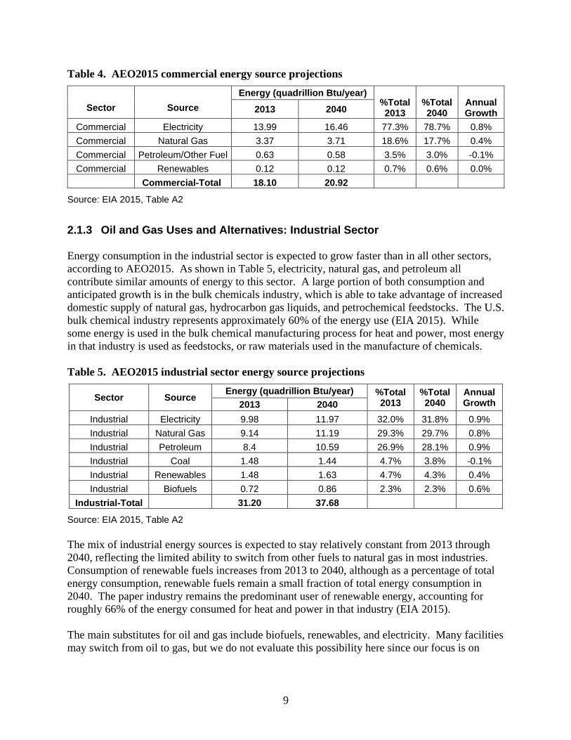
2.1.3 Oil and Gas Uses and Alternatives: Industrial Sector

Energy consumption in the industrial sector is expected to grow faster than in all other sectors,

according to AEO2015. As shown in Table 5, electricity, natural gas, and petroleum all

contribute similar amounts of energy to this sector. A large portion of both consumption and

anticipated growth is in the bulk chemicals industry, which is able to take advantage of increased

domestic supply of natural gas, hydrocarbon gas liquids, and petrochemical feedstocks. The U.S.

bulk chemical industry represents approximately 60% of the energy use (EIA 2015). While

some energy is used in the bulk chemical manufacturing process for heat and power, most energy

in that industry is used as feedstocks, or raw materials used in the manufacture of chemicals.

Table 5. AEO2015 industrial sector energy source projections

Sector Source Energy (quadrillion Btu/year) %Total

2013 %Total 2040

Annual Growth 2013 2040

Industrial Electricity 9.98 11.97 32.0% 31.8% 0.9%

Industrial Natural Gas 9.14 11.19 29.3% 29.7% 0.8%

Industrial Petroleum 8.4 10.59 26.9% 28.1% 0.9%

Industrial Coal 1.48 1.44 4.7% 3.8% -0.1%

Industrial Renewables 1.48 1.63 4.7% 4.3% 0.4%

Industrial Biofuels 0.72 0.86 2.3% 2.3% 0.6%

Industrial-Total 31.20 37.68


The mix of industrial energy sources is expected to stay relatively constant from 2013 through

2040, reflecting the limited ability to switch from other fuels to natural gas in most industries.

Consumption of renewable fuels increases from 2013 to 2040, although as a percentage of total

energy consumption, renewable fuels remain a small fraction of total energy consumption in

2040. The paper industry remains the predominant user of renewable energy, accounting for

roughly 66% of the energy consumed for heat and power in that industry (EIA 2015).

The main substitutes for oil and gas include biofuels, renewables, and electricity. Many facilities

may switch from oil to gas, but we do not evaluate this possibility here since our focus is on

10

shifts from oil and gas to other fuel sources. There is also the possibility of recycled plastic and

biobased chemicals being used as substitutes for plastic manufacturing.

2.1.4 Oil and Gas Uses and Alternatives: Transportation Sector

As shown in Table 6, petroleum products are predominantly used in the transportation sector and

make up the majority of the energy used in this sector. The only significant substitutes for

petroleum products in this sector are natural gas and more efficient vehicles. Greater fuel

efficiency should be achieved in all of the transportation modes. In the near term, efficiency of

the U.S. vehicle fleet is likely to be determined more by stricter regulatory requirements than by

a demand from consumers for more efficient vehicles. The corporate average fuel economy

(CAFE) standards will continue to require cars and trucks to be more fuel efficient over the next

several decades. Gasoline-only vehicles, excluding hybridization or flex-fuel capabilities,

represent about 46% of the total new sales in 2040. However, alternative fuel vehicles and

vehicles with hybrid technologies show a significant growth in the market: gasoline vehicles

with micro hybrid systems represent about 33%, E85 flexible-fuel vehicles (FFVs) 10%, full

hybrid electric vehicles 5%, diesel vehicles 4%, and plug-in hybrid vehicles and electric vehicles

2% (EIA 2015).

The increased use of compressed natural gas and liquefied natural gas in vehicles represents

close to 3% of the total energy use in the transportation sector.

Table 6. AEO2015 transportation sector energy source projections

Sector Source

Energy (quadrillion Btu/year)

%Total 2013

%Total 2040

Annual Growth

2013 2040

Transportation Petroleum 26 24.76 96.3% 93.0% -0.2%

Transportation Pipeline Fuel Natural Gas 0.88 0.96 3.3% 3.6% 0.3%

Transportation Electricity 0.07 0.18 0.3% 0.7% 3.4%

Transportation Compressed/Liquefied

Natural Gas 0.05 0.71 0.2% 2.7% 10.3%

Transportation Liquid Hydrogen 0 0 0.0% 0.0% 0.0%

Transportation-Total

27.00 26.61


2.1.5 Oil and Gas Uses and Alternatives: Electricity

Table 7 presents the fuels used to produce electricity and the amount of fuel used in 2013 and

projected to be used in 2040. Petroleum, the only fuel projected to decrease in usage, is not used

in a significant amount in fueling power plants. The absolute value of this decrease is

insignificant compared to the use of petroleum in the transportation and industrial sectors.

Generation from coal-fired plants and nuclear energy sources remains fairly flat into 2040.

Renewables have the highest projected growth in terms of percentage and have a similar absolute

growth as natural gas. Renewables will be an important substitute for natural gas, but both

11

renewables and natural gas will make up most of the capacity decrease resulting from the slower

growth in the coal and nuclear industries. Climate change and energy policy could have a

significant effect on shaping the electricity sector; Table 7 assumes that current laws and

regulations affecting the energy sector remain unchanged through 2040.

Table 7. AEO2015 electricity fuel projections

Fuel Energy-billion kilowatt-hours % Total

2013 % Total

2040 Annual Growth

2013 2040

Coal 1586 1702 39.0% 33.7% 0.30%

Natural Gas 1118 1569 27.5% 31.0% 1.30%

Renewables 530 909 13.0% 18.0% 2.00%

Nuclear 789 833 19.4% 16.5% 0.20%

Other 20 25 0.5% 0.5% 0.80%

Petroleum 27 18 0.7% 0.4% -1.60%

Total 4070 5056


Tables 1–5 do not identify the specific renewables that are expected to contribute to the increase

in capacity. AEO2015 makes the following comment regarding renewable growth and provides

additional details on renewables and their growth projections.

Solar photovoltaic (PV) technology is the fastest-growing energy source for

renewable generation, at an annual average rate of 6.8%. Wind energy accounts

for the largest absolute increase in renewable generation and for 40.0% of the

growth in renewable generation from 2013 to 2038, displacing hydropower and

becoming the largest source of renewable generation by 2040. Geothermal

generation grows at an average annual rate of about 5.5% over the projection

period, but because geothermal resources are concentrated geographically, the

growth is limited to the western United States. Biomass generation increases by

an average of 3.1%/year, led by cofiring at existing coal plants through about

2030. After 2030, new dedicated biomass plants account for most of the growth

in generation from biomass energy sources.

It should be noted that onshore wind energy accounts for the largest share of the projected wind

energy increase.

2.2 CURRENT AND FUTURE PRODUCTION OF ENERGY SOURCES

2.2.1 Current and Future Energy Use

Section 2 presents more detailed information on each of the potential energy substitutes,

including generation amounts and U.S. locations where these energy sources are generated.

Figure 1 presents the percentage of 2013 energy consumption in the United States by energy

source, as well as projections of energy consumption through 2040 (EIA 2015). This figure

12

indicates that there is little change in the percentage of total national energy production for liquid

biofuels, nuclear, and coal from 2013 to 2040. Renewables increase from 8% to 10%, natural

gas increases from 27% to 29%, and petroleum and other liquids decreases from 36% to 33%.

Source: EIA 2015, p. 24, Figure 31

Figure 1. Primary energy consumption by fuel in the reference case,

1980–2040 (quadrillion Btu)

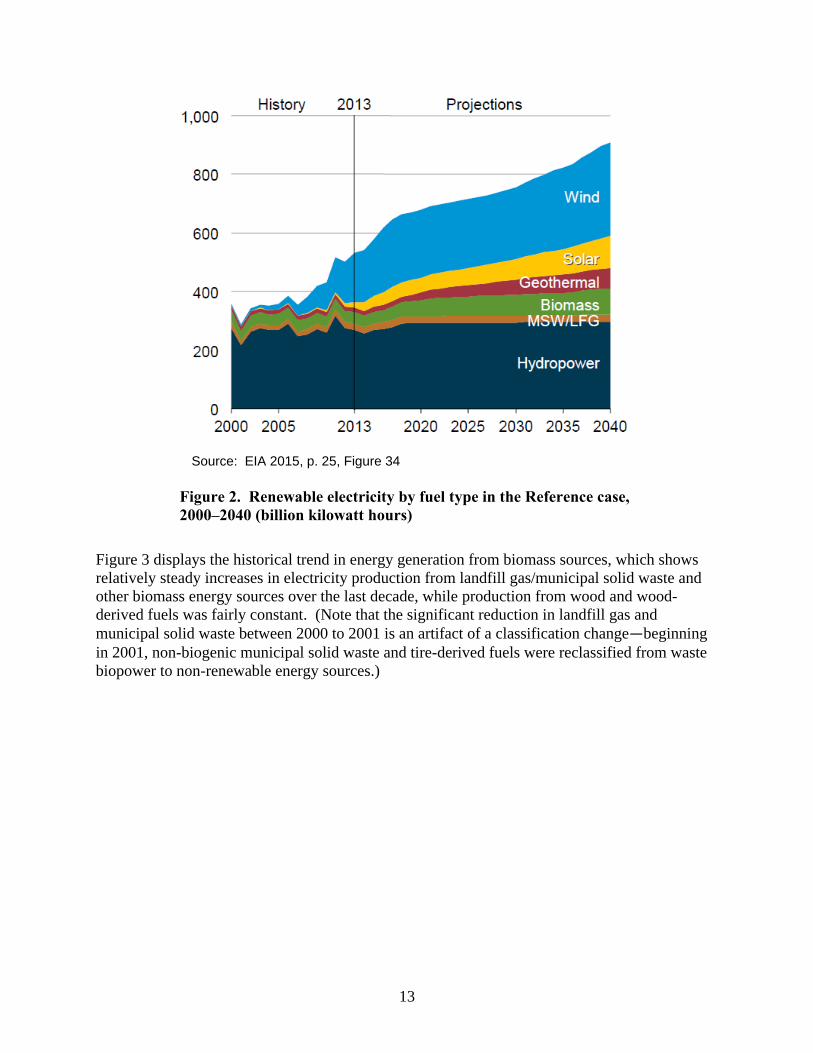
2.2.2 Renewable Energy Current and Future Use

Electricity generation from both wind and solar energy has seen significant increases over the

last several years, while production of other renewable energy sources has remained relatively

stable. Figure 2 shows electricity generation by renewable fuel in the AEO2015 Reference case,

2000–2040, indicating that renewables increase to 18% of the total fuel source in 2040 and in

fact surpass nuclear energy. Figure 2 shows the renewable electricity generation by fuel type per

the AEO2015 Reference case. This figure shows the continued growth of wind and solar, along

with an increase in geothermal as an energy source. Hydropower and biomass are projected to

contribute similar amounts of energy in 2040 as in 2013.

13

Source: EIA 2015, p. 25, Figure 34

Figure 2. Renewable electricity by fuel type in the Reference case,

2000–2040 (billion kilowatt hours)

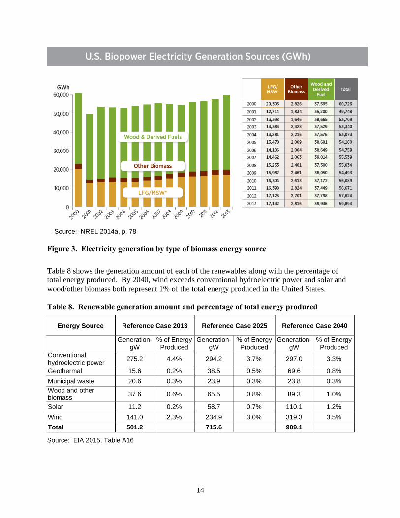
Figure 3 displays the historical trend in energy generation from biomass sources, which shows

relatively steady increases in electricity production from landfill gas/municipal solid waste and

other biomass energy sources over the last decade, while production from wood and wood-

derived fuels was fairly constant. (Note that the significant reduction in landfill gas and

municipal solid waste between 2000 to 2001 is an artifact of a classification change—beginning

in 2001, non-biogenic municipal solid waste and tire-derived fuels were reclassified from waste

biopower to non-renewable energy sources.)

14

Source: NREL 2014a, p. 78

Figure 3. Electricity generation by type of biomass energy source

Table 8 shows the generation amount of each of the renewables along with the percentage of

total energy produced. By 2040, wind exceeds conventional hydroelectric power and solar and

wood/other biomass both represent 1% of the total energy produced in the United States.

Table 8. Renewable generation amount and percentage of total energy produced

Energy Source Reference Case 2013 Reference Case 2025 Reference Case 2040

Generation-

gW % of Energy

Produced Generation-

gW % of Energy

Produced Generation-

gW % of Energy

Produced

Conventional hydroelectric power

275.2 4.4% 294.2 3.7% 297.0 3.3%

Geothermal 15.6 0.2% 38.5 0.5% 69.6 0.8%

Municipal waste 20.6 0.3% 23.9 0.3% 23.8 0.3%

Wood and other biomass

37.6 0.6% 65.5 0.8% 89.3 1.0%

Solar 11.2 0.2% 58.7 0.7% 110.1 1.2%

Wind 141.0 2.3% 234.9 3.0% 319.3 3.5%

Total 501.2 715.6 909.1


15

The International Renewable Energy Agency (IRENA) recently produced an alternative forecast

for renewable energy in the United States (IRENA 2015).2 Unlike the AEO2015 business-as-

usual projections, IRENA forecasts the effects of potential future new investments and policies

targeting support for renewable energy. According to IRENA’s “REmap” analysis, the United

States could reach a 27% renewable energy share by 2030 if the realizable potential of all the

analyzed renewable energy technologies is implemented.

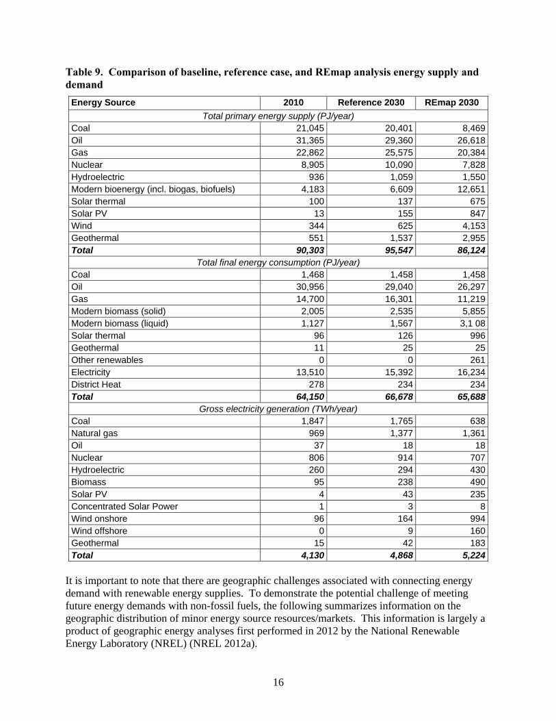
Table 9 presents a summary comparing the REmap analysis energy production projections with

the Annual Energy Outlook 2013 (current version at the time of the REmap work) (EIA 2003, or

AEO2013) Reference case projections. Under REmap, wind and biomass accounts for nearly

three-quarters of the total renewable energy use in 2030, and wind accounts for over two-thirds

of total power sector energy. The remainder of REmap’s 2030 energy production is equally

divided between biomass, solar, and geothermal.

The REmap analysis also projects total biomass use to increase three-fold from 2010, with

biomass accounting for more than half of total renewable energy use in 2030. The analysis

concentrates additional biomass use in heating markets (buildings and industry). Although

biomass may be the largest source of renewable energy in REmap 2030, wind, solar, and

geothermal energy show the highest growth rates.

2 IRENA is an intergovernmental organization that supports countries in their transition to a sustainable

energy future. IRENA promotes the widespread adoption and sustainable use of all forms of renewable energy,

including bioenergy, geothermal, hydropower, ocean, solar, and wind energy, in the pursuit of sustainable

development, energy access, energy security, and low-carbon economic growth and prosperity.

16


demand

Energy Source 2010 Reference 2030 REmap 2030

Total primary energy supply (PJ/year)

Coal 21,045 20,401 8,469

Oil 31,365 29,360 26,618

Gas 22,862 25,575 20,384

Nuclear 8,905 10,090 7,828

Hydroelectric 936 1,059 1,550

Modern bioenergy (incl. biogas, biofuels) 4,183 6,609 12,651

Solar thermal 100 137 675

Solar PV 13 155 847

Wind 344 625 4,153

Geothermal 551 1,537 2,955

Total 90,303 95,547 86,124

Total final energy consumption (PJ/year)

Coal 1,468 1,458 1,458

Oil 30,956 29,040 26,297

Gas 14,700 16,301 11,219

Modern biomass (solid) 2,005 2,535 5,855

Modern biomass (liquid) 1,127 1,567 3,1 08

Solar thermal 96 126 996

Geothermal 11 25 25

Other renewables 0 0 261

Electricity 13,510 15,392 16,234

District Heat 278 234 234

Total 64,150 66,678 65,688

Gross electricity generation (TWh/year)

Coal 1,847 1,765 638

Natural gas 969 1,377 1,361

Oil 37 18 18

Nuclear 806 914 707

Hydroelectric 260 294 430

Biomass 95 238 490

Solar PV 4 43 235

Concentrated Solar Power 1 3 8

Wind onshore 96 164 994

Wind offshore 0 9 160

Geothermal 15 42 183

Total 4,130 4,868 5,224

It is important to note that there are geographic challenges associated with connecting energy

demand with renewable energy supplies. To demonstrate the potential challenge of meeting

future energy demands with non-fossil fuels, the following summarizes information on the

geographic distribution of minor energy source resources/markets. This information is largely a

product of geographic energy analyses first performed in 2012 by the National Renewable

Energy Laboratory (NREL) (NREL 2012a).

17

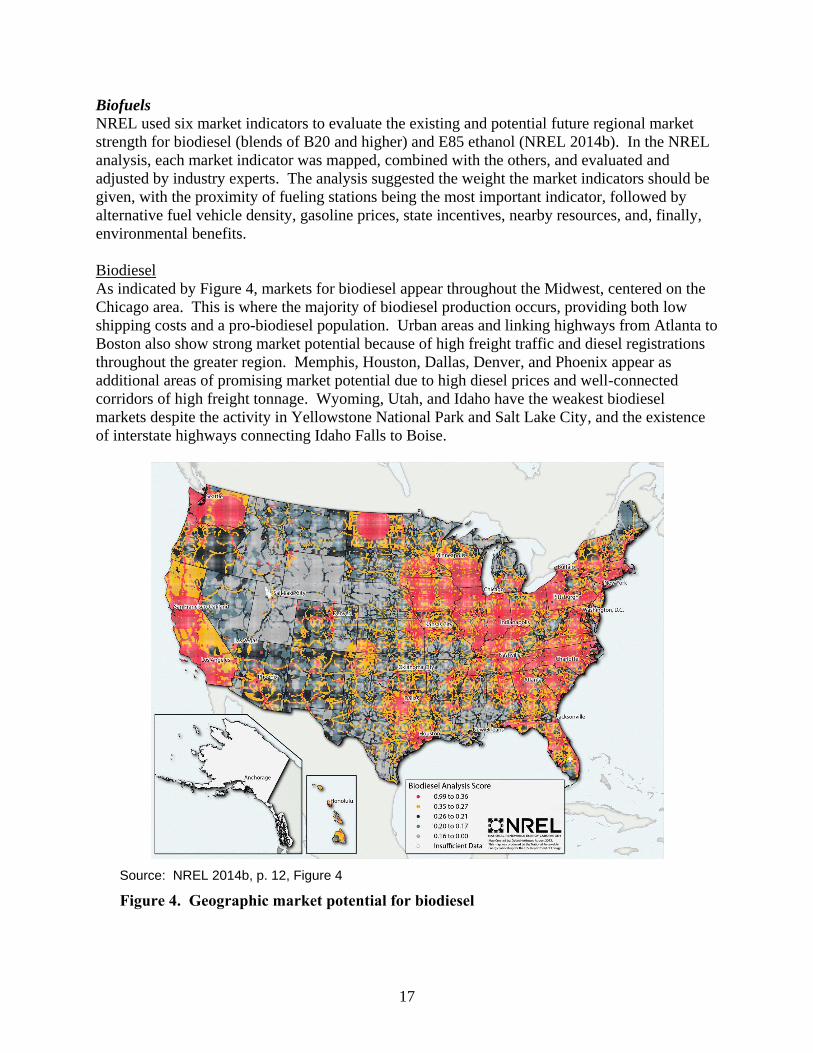
Biofuels

NREL used six market indicators to evaluate the existing and potential future regional market

strength for biodiesel (blends of B20 and higher) and E85 ethanol (NREL 2014b). In the NREL

analysis, each market indicator was mapped, combined with the others, and evaluated and

adjusted by industry experts. The analysis suggested the weight the market indicators should be

given, with the proximity of fueling stations being the most important indicator, followed by

alternative fuel vehicle density, gasoline prices, state incentives, nearby resources, and, finally,

environmental benefits.

Biodiesel

As indicated by Figure 4, markets for biodiesel appear throughout the Midwest, centered on the

Chicago area. This is where the majority of biodiesel production occurs, providing both low

shipping costs and a pro-biodiesel population. Urban areas and linking highways from Atlanta to

Boston also show strong market potential because of high freight traffic and diesel registrations

throughout the greater region. Memphis, Houston, Dallas, Denver, and Phoenix appear as

additional areas of promising market potential due to high diesel prices and well-connected

corridors of high freight tonnage. Wyoming, Utah, and Idaho have the weakest biodiesel

markets despite the activity in Yellowstone National Park and Salt Lake City, and the existence

of interstate highways connecting Idaho Falls to Boise.

Source: NREL 2014b, p. 12, Figure 4

Figure 4. Geographic market potential for biodiesel

18

Geographic areas identified by NREL with unexpected biodiesel market strength include North

Dakota and the Oklahoma panhandle, where biodiesel refineries and a high number of state

incentives push market ratings into high categories.

North Carolina has many pro-biodiesel incentives and a disproportionate number of B20

refueling stations (18% of the nation’s total, despite only having 3% of the total U.S.

population). These refueling stations are well-dispersed throughout the state. Pennsylvania

shows great promise due to high gasoline prices, freight tonnage, diesel vehicle registrations, and

a number of biodiesel refineries. Hawaii is strong as well due to very high gasoline prices, many

state incentives, a high density of diesel registrations, and seven B20 stations. However, the lack

of biodiesel supply is currently overriding these indicators of high demand. The Appalachian

region has poor biodiesel market potential even though it is surrounded by relatively strong

biodiesel markets.

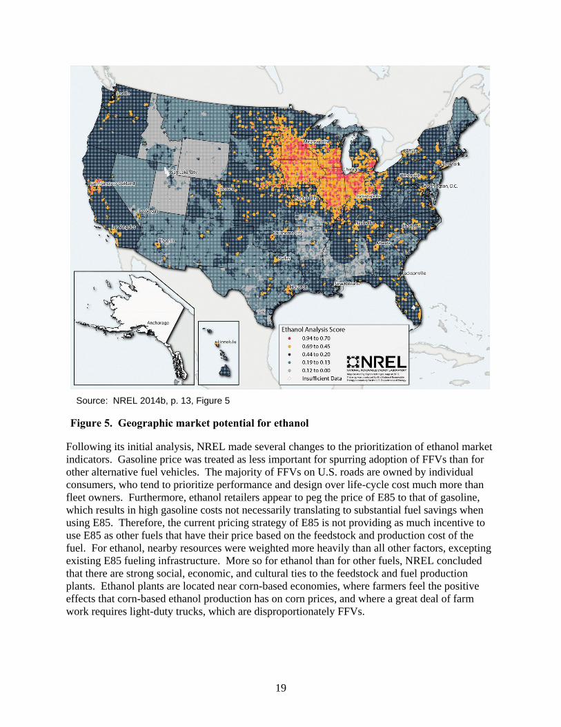
Ethanol

The NREL analysis found that ethanol markets are most robust in the Midwest (see Figure 5).

Outside the Midwest, the urban areas surrounding the San Francisco Bay (including

Sacramento), Los Angeles, Denver, New York City, Rochester-Buffalo, Houston, Miami, and

Dallas have large markets (listed in order of the size of the geographic area that received scores

in the highest quintile). The weakest ethanol markets are found in the region comprising

Wyoming, Utah, Idaho, Nevada, and Montana. These states have very few pro-ethanol

incentives, low FFV density, few fueling stations, and only one ethanol refinery.

19

Source: NREL 2014b, p. 13, Figure 5

Figure 5. Geographic market potential for ethanol

Following its initial analysis, NREL made several changes to the prioritization of ethanol market

indicators. Gasoline price was treated as less important for spurring adoption of FFVs than for

other alternative fuel vehicles. The majority of FFVs on U.S. roads are owned by individual

consumers, who tend to prioritize performance and design over life-cycle cost much more than

fleet owners. Furthermore, ethanol retailers appear to peg the price of E85 to that of gasoline,

which results in high gasoline costs not necessarily translating to substantial fuel savings when

using E85. Therefore, the current pricing strategy of E85 is not providing as much incentive to

use E85 as other fuels that have their price based on the feedstock and production cost of the

fuel. For ethanol, nearby resources were weighted more heavily than all other factors, excepting

existing E85 fueling infrastructure. More so for ethanol than for other fuels, NREL concluded

that there are strong social, economic, and cultural ties to the feedstock and fuel production

plants. Ethanol plants are located near corn-based economies, where farmers feel the positive

effects that corn-based ethanol production has on corn prices, and where a great deal of farm

work requires light-duty trucks, which are disproportionately FFVs.

20

Biomass

As indicated in Figure 6, the regions that show with the most biomass potential are in the

Midwest for crops, and the West/South for forest residues.

Source: NREL 2014c

Figure 6. Geographic market potential for biomass energy

21

Geothermal

Geothermal resources are primarily centered in the western United States. (see Figure 7). The

Rocky Mountain States, and the Great Basin particularly, contain the most favorable resources.

It should be noted that, especially in western states, a considerable portion of geothermal

resources occur on protected land.

Source: NREL 2009

Figure 7. Geographic market potential for geothermal energy

Hydroelectric

Hydropower is currently the largest source of renewable power generation; however, it is

expected to be overtaken by wind power due to the limited potential for new large-scale

hydroelectric power plants. Figure 8 displays the estimated capacity for the top non-powered

dams in the United States. Additional potential capacity can be assumed to be available from

retrofitting and upgrading turbines at existing hydroelectric dams.

22

Source: NREL no date

Figure 8. Top non-powered dams with hydroelectric energy potential

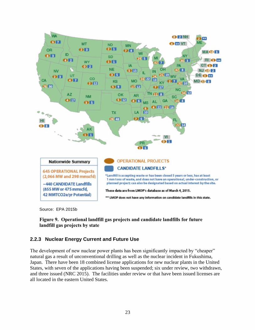
Municipal Waste

Approximately one quarter of the currently operating landfill gas projects are using the energy

produced to directly offset the use of other fuels such as natural gas, coal, or fuel oil (EPA

2015a). Energy production from landfill gas can be achieved through the use of various

technologies, making it an option for large-scale as well as small-scale applications. Currently,

the ability for landfill gas to be converted into other types of fuels (liquefied natural gas, high- or

medium-Btu fuel, or methanol) is under investigation. Figure 9 gives the number of operational

landfill gas projects as well as the number of identified candidate landfills for future projects in

each state as of March 2015.

23

Source: EPA 2015b

Figure 9. Operational landfill gas projects and candidate landfills for future

landfill gas projects by state

2.2.3 Nuclear Energy Current and Future Use

The development of new nuclear power plants has been significantly impacted by “cheaper”

natural gas a result of unconventional drilling as well as the nuclear incident in Fukushima,

Japan. There have been 18 combined license applications for new nuclear plants in the United

States, with seven of the applications having been suspended; six under review, two withdrawn,

and three issued (NRC 2015). The facilities under review or that have been issued licenses are

all located in the eastern United States.

24

2.2.4 Other Natural Gas Current and Future Use

NREL has developed a map of the potential county-level generation of methane from biomass

gas resources. This map, which is presented as Figure 10, generally indicates the greatest

resources in heavily populated metropolitan areas and areas with substantial livestock

production.

Source: NREL 2014d

Figure 10. Geographic market potential for biomass gas

2.2.5 Location of Solar Energy Facilities/Opportunities in the United States

NREL has produced two maps characterizing the geographic distribution of solar resources.

Figure 11 presents Concentrating Solar Resources (CSR), while Figure 12 displays PV resources.

Technical potential for CSR exists predominately in the Southwest. This pattern holds for the

potential for PV solar energy, although the NREL analysis indicates much less of a decline from

the Southwest region’s potential to the South Central and Southeast regions than indicted by the

potential for CSR.

25

Source: NREL 2012b

Figure 11. Geographic market potential for concentrating solar resources

26

Source: NREL 2012c

Figure 12. Geographic market potential for PV solar resources

2.2.6 Location of wind Energy Facilities in the United States

The potential for onshore wind energy is greatest in the western and central Great Plains and

lowest in the southeastern United States (see Figure 13). Areas in the Midwest routinely average

wind speeds of 8.5 meters per second at a height of 80 meters. The ability to deliver electricity

to consumers from these high resource areas, which are often far from consumption centers, can

prove a challenge given the existing grid infrastructure. Technical potential for offshore wind

power is present in significant quantities in all offshore regions of the United States. Wind

speeds off the Atlantic Coast and in the Gulf of Mexico are lower than they are off the Pacific

Coast, but the presence of shallower waters there makes these regions more attractive for

development.

27

Source: NREL 2011

Figure 13. Geographic market potential for wind energy

2.3 ENVIRONMENTAL AND SOCIAL COSTS OF ENERGY SOURCES

2.3.1 Overview of Environmental and Social Costs of Energy Sources

This section focuses on the potential environmental costs associated with the primary alternatives

to oil and gas. The OECM considers “main” energy market substitutions (i.e., increased imports

and onshore production of oil and natural gas, fuel switching to coal, and reduced demand), but

multiple other “minor” energy substitutes exist (e.g., nuclear, wind, and solar electricity;

biofuels). This section provides a qualitative discussion of the environmental and social costs of

both the main energy substitutes not already monetized in the OECM and minor energy

substitutes. The OECM addresses the following environmental and social costs:

Recreation

Air quality

Property values

Subsistence use

Commercial fishing

28

Ecological effects

The purpose of this section is not to explore this subject in great detail. Rather, we make the

point that negative as well as positive externalities (i.e., costs borne by society that are not

reflected in a good’s price) can be attributed to all forms of energy production, and any complete

consideration of alternatives would seek to take these costs into account. An exception could be

made when increased energy efficiency, or simple conservation, are the oil or gas substitutes, as

those actions often will result in decreased use of the energy resources that give rise to

environmental costs.

The primary alternatives to the direct use of oil and gas across all sectors are biofuels and

electricity production for heat or for stationary or mobile power, using non-hydrocarbon fuel

sources (i.e., coal, fissionable materials, or renewable resources). All energy sources have

externalities.

The following activities are assumed to be the most significant in terms of potential

environmental and social costs not addressed in the OECM or associated with the minor energy

sources: (1) waste management issues, in particular with the nuclear and coal industry;

(2) health and safety issues with the mining of coal and uranium; (3) groundwater impacts

potentially associated with onshore oil and gas production; (4) surface water impacts from spills

at onshore energy-producing facilities; (5) the air quality impacts of incremental emissions

associated with biofuels (air quality impacts from traditional energy sources are covered in

OECM); (6) socioeconomic issues associated with the loss of land from mining or processing

activities, as well as the impacts to real estate values near energy production facilities;

(7) ecological and wildlife impacts associated with all onshore energy production and offshore

renewable energy production; and (8) the spill impacts from onshore energy production.

2.3.2 Waste Management

Waste management issues are also a concern, with the biggest concern being associated with

nuclear power and coal-fired power plants. The country has been struggling for decades to

determine how the spent fuel from the nuclear power plants will be managed on a long-term

basis. The U.S. Department of Energy (DOE) has spent roughly $12 billion on Yucca Mountain

without a facility being constructed (NYT 2011). If a decision were made to proceed with

construction of the facility, the total cost would be about $100 billion.

On December 22, 2008, the walls of a dam holding 1.1 billion gallons of coal ash crumbled,

spilling the material into the town of Kingston, Tennessee, and creating the largest industrial spill

in U.S. history. The ash (waste residuals from burning coal mixed with water) wiped out roads,

crumpled docks, and destroyed homes. In excess of $1 billion has been spent to address this

incident (USAToday 2013).

On February 2, 2014, a release of coal ash into the Dan River occurred at the Dan River Steam

Station (Duke Energy) north of Eden, North Carolina. It is estimated that costs to remediate this

spill will be roughly $15 million (HP 2015).

29

2.3.3 Mining Health and Safety

Both the coal and nuclear industries rely on a fuel source that is mined. Health and safety issues

associated with these mining activities are discussed below.

The U.S. Department of Labor (DOL) has tracked fatalities associated with coal mining since

1900 (DOL 2015). From 1900 through 1930, there were typically about 2,000 deaths per year

associated with mining. From 1931 through 1948, the typical number of deaths had decreased to

about 1,000 per year. From 1949 through 1984, the number had been reduced to the

approximate range of 100 to 500 deaths per year. The annual fatalities have continued to

decrease and have recently been in the range of 20 per year.

Research accumulated against coal has shown that human health impacts from coal emissions on

miners, workers, and local communities are severe. The release of heavy metal and organic

compounds pose major health risks. Among health risks are lung cancer, bronchitis, heart

disease, and other health conditions.

The fuel for nuclear power plants, uranium, is also mined. Uranium mining is believed to be the

cause of a statistically significant amount of lung cancers as a result of exposure of the miners to

radon based on some epidemiological studies. While these studies are not conclusive, the

industry has taken steps to improve ventilation and reduce the radon content in the mines.

2.3.4 Groundwater Impacts

Many onshore energy-producing activities have the potential to contaminate groundwater.

Unconventional drilling for oil and gas, if not performed properly, has the potential to

contaminate groundwater. Groundwater contamination can prevent the local community from

using the groundwater for drinking and can cause other threats to human health and the

environment if the groundwater is withdrawn and used or upon its discharge to a surface water.

Groundwater contamination is one of the key items that will cause sites to become Superfund

sites and require millions of dollars to remediate.

2.3.5 Surface Water Impacts

Surface water impacts are a specific concern for on-shore energy production. According to an

EPA report released June 4, 2015 (EPA 2015c), groundwater withdrawals used for hydraulic

fracturing that exceed the land’s natural recharge rates decrease water storage in aquifers and can

potentially mobilize contaminants or allow the infiltration of lower quality water from the land

surface. Additionally, a general decrease in groundwater being discharged to streams can also

affect surface water quality.

EPA (2015c) also characterized 151 spills due to hydraulic fracturing (fracking). In about 9%, or

13, of those spills, fluids reached surface water. These spills have the potential to contaminate

drinking water resources, possibly affecting human health.

30

On November 2010, an estimated 6,300 to 57,000 gallons of Marcellus Shale produced water

was illegally discharged at XTO Energy Inc.’s Marquardt pad and flowed into the Susquehanna

River watershed. Although no impacts to water wells and springs were observed within one mile

at the last sampling, produced water constituents could eventually reach drinking water sources

through surface runoff or infiltration to the ground (EPA 2015c).

Hydroelectric facilities can have major impacts on aquatic ecosystems if proper actions are not

taken (e.g., fish ladders and intake screens). If these actions are not taken, fish and other

organisms can be injured and killed by turbine blades. In addition to direct contact with the

turbine blades, there can also be wildlife impacts both from the damned reservoirs and

downstream from the facility. Reservoir water is usually more stagnant than normal river water

and will therefore have higher than normal amounts of sediments and nutrients, which can

cultivate an excess of algae and other aquatic weeds. These weeds can crowd out other river

animal and plant life.

2.3.6 Air Quality Impacts Air emissions can jeopardize a region’s ability to maintain or achieve attainment status, be

harmful to the health of the local population, increase greenhouse gas emissions, and also present

a safety hazard (e.g., release of methane into confined spaces). From a life-cycle perspective, all

of the energy sources will contribute air emissions, with most of the renewables having

negligible to no air emissions during operations and coal having the greatest amount of air

emissions during its life-cycle. In just one year, 50,000 U.S. deaths can be attributed to air

pollution from coal-fired power generation, while death counts reach over 200,000 per year

globally (Flannery and Stanley 2014).

With nuclear power, small amounts of radioactivity are released, including small quantities of

radioactive gases (krypton-85, xenon-13, and iodine-131). These gases may be detectible but are

never at harmful levels (WNA 2013).

Contributing significantly more to pollution, fracking emits unhealthy levels of smog and toxic

air contaminants. Exposure to such pollutants can cause eye, nose, and throat irritation,

respiratory illnesses, central nervous system damage, birth defects, cancer, or premature death.

Preliminary results from a study in Pennsylvania, for example, show impacts among newborns

that could be linked to air pollution such as increases in low birth weight. Additionally,

researchers who looked at air pollution levels near fracking sites in Colorado found an increase

in chronic and sub-chronic effects stemming mainly from oil and gas pollutants which have the

capability to harm the respiratory and neurological system, leading to symptoms like shortness of

breath, nosebleeds, headaches, dizziness, and chest tightness (NRDC 2014).

One of the renewables that has the potential to impact air quality is biofuels. Most studies have

found that producing first-generation biofuels from current feedstocks results in emission

reductions in the range of 20%–60% relative to fossil fuels, provided the most efficient systems

are used and carbon releases deriving from land-use change are excluded (GF 2015). Brazil,

which has extensive experience of producing ethanol from sugar cane, shows even greater

reductions. Second-generation biofuels, although still insignificant at the commercial level,

31

typically offer emission reductions between 70%–90%, compared with fossil diesel and petrol

(excluding carbon releases related to land-use change).

2.3.7 Socioeconomic Impacts

A study performed in 2010 indicated that there can be a 3%–7% decrease in housing values for

neighborhoods located within 2 miles of a power plant compared to neighborhoods with similar

housing and demographic characteristics (Davis 2010). The report mentions some evidence that

there are larger decreases from homes located within a mile of a plant.

Eastern Kentucky and its coal industry seem to pose a similar issue. According to the

Appalachian Regional Commission, there is a relationship between coal-dependent economies

and undiversified economies, fewer professional service employment position, and lower

educational attainment. The disadvantages the Appalachian region of the United States have

long been associated with poor public health outcomes within the surrounding population,

making the costs outweigh the benefits in the region (ARC/USDA 2010).

2.3.8 Ecological and Wildlife Impacts One of the most mentioned wildlife impacts of power plants is associated with onshore wind

turbines. A recent study in which researchers used 58 mortality estimates that met their criteria

estimates that between 140,000 and 328,000 birds die each year from collisions with monopole

turbines, which now comprise the vast majority of U.S. wind turbines (Loss et al. 2013).

Another study concludes that about 368,000 fatalities for all bird species are caused annually by

collisions with wind turbines (Erikson et al. 2014).

Wildlife impacts associated with onshore oil (pipelines) include fragmentation of land.

Depending on scale, these constructions and installations may cause displacement of wildlife,

along with deforestation and general distortion of the terrestrial landscape. Additionally, the

discharge and disposal of wastes from onshore operation installations may harm the surrounding

land and its habitats, resulting in death of fauna and flora. Spills associated with pipelines and

onshore oil have the potential to destroy acres of land along with its inhabitants (Ramirez and

Mosley 2015).

2.3.9 Onshore Spills The largest onshore oil spill in U.S. history occurred on July 26, 2010. Enbridge’s pipeline

ruptured and released nearly 3 million liters of tar sands diluted bitumen into a tributary of the

Kalamazoo River in Michigan. Final costs of $1.04 billion include cleanup and remediation,

along with a fine levied by the Pipeline and Hazardous Materials Safety Administration.

Communities along the creek inlet and the river experienced sickness from the fumes that

blanketed miles of intersecting wetlands and waterways. The spill contaminated 20 miles of the

river and local drinking water supply, and more than 50 homes near the site were evacuated

(NWF 2010).

32

Earlier, on June 12, 2010, 33,600 gallons of oil leaked from the Chevron Oil Co. pipeline on its

way to the nearby refinery. Although the oil was stopped before it ran into the Great Salt Lake,

approximately 200 birds were coated with oil (NWF 2010).

Pipeline spills have also been known to cause casualties. In November of 2007, two people were

killed, seven injured, and four homes were destroyed after 430,000 gallons of liquid propane

were released in Carmichael, Mississippi from a ruptured pipeline. Additionally, 70 acres of

woodland were devastated in the process (NWF 2010).

One of the energy sources that has been associated with spills is the unconventional drilling

(fracking) of oil and gas. Roughly 865,000 gallons of oil spilled from a Tesoro Logistics

pipeline in Tioga, North Dakota, in September 2013 (DESMOG 2013). The pipeline was

carrying oil from a fracking operation to a rail facility. The estimate to clean up this spill was

$4 million.

More recently, in January 2015, 3 million gallons of a brine from a fracking operation spilled in

western North Dakota (PBS 2015). The leak reached the Missouri River and contaminated two

creeks near Williston—Blacktail Creek and the Little Muddy River. The Little Muddy River

empties into the Missouri River, one of the town’s sources of drinking water. There have been

conflicting reports on the presence of any threats to human health and the environment from the

spill, although it was the largest saltwater spill in North Dakota history.

2.3.10 Environmental and Social Impacts by Energy Source

The tables that follow summarize environmental and social costs into the following categories:

Air impacts

Geologic impacts

Health and human safety impacts

Land use impacts

Noise impacts

Socioeconomic impacts

Transportation impacts

Vegetation impacts

Visual resource Impacts

Waste management impacts

Water resources impacts

Wildlife impacts

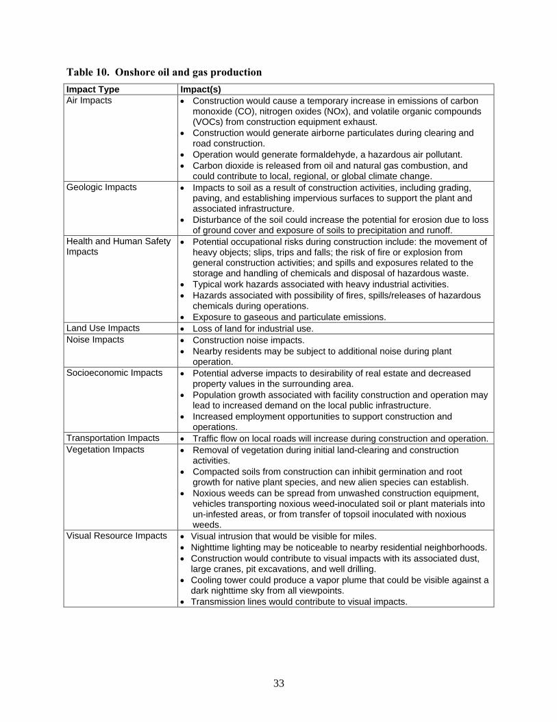
33

Table 10. Onshore oil and gas production

Impact Type Impact(s)

Air Impacts Construction would cause a temporary increase in emissions of carbon monoxide (CO), nitrogen oxides (NOx), and volatile organic compounds (VOCs) from construction equipment exhaust.

Construction would generate airborne particulates during clearing and road construction.

Operation would generate formaldehyde, a hazardous air pollutant.

Carbon dioxide is released from oil and natural gas combustion, and could contribute to local, regional, or global climate change.

Geologic Impacts Impacts to soil as a result of construction activities, including grading, paving, and establishing impervious surfaces to support the plant and associated infrastructure.

Disturbance of the soil could increase the potential for erosion due to loss of ground cover and exposure of soils to precipitation and runoff.

Health and Human Safety Impacts

Potential occupational risks during construction include: the movement of heavy objects; slips, trips and falls; the risk of fire or explosion from general construction activities; and spills and exposures related to the storage and handling of chemicals and disposal of hazardous waste.

Typical work hazards associated with heavy industrial activities.

Hazards associated with possibility of fires, spills/releases of hazardous chemicals during operations.

Exposure to gaseous and particulate emissions.

Land Use Impacts Loss of land for industrial use.

Noise Impacts Construction noise impacts.

Nearby residents may be subject to additional noise during plant operation.

Socioeconomic Impacts Potential adverse impacts to desirability of real estate and decreased property values in the surrounding area.

Population growth associated with facility construction and operation may lead to increased demand on the local public infrastructure.

Increased employment opportunities to support construction and operations.

Transportation Impacts Traffic flow on local roads will increase during construction and operation.

Vegetation Impacts Removal of vegetation during initial land-clearing and construction activities.

Compacted soils from construction can inhibit germination and root growth for native plant species, and new alien species can establish.

Noxious weeds can be spread from unwashed construction equipment, vehicles transporting noxious weed-inoculated soil or plant materials into un-infested areas, or from transfer of topsoil inoculated with noxious weeds.

Visual Resource Impacts Visual intrusion that would be visible for miles.

Nighttime lighting may be noticeable to nearby residential neighborhoods.

Construction would contribute to visual impacts with its associated dust, large cranes, pit excavations, and well drilling.

Cooling tower could produce a vapor plume that could be visible against a dark nighttime sky from all viewpoints.

Transmission lines would contribute to visual impacts.

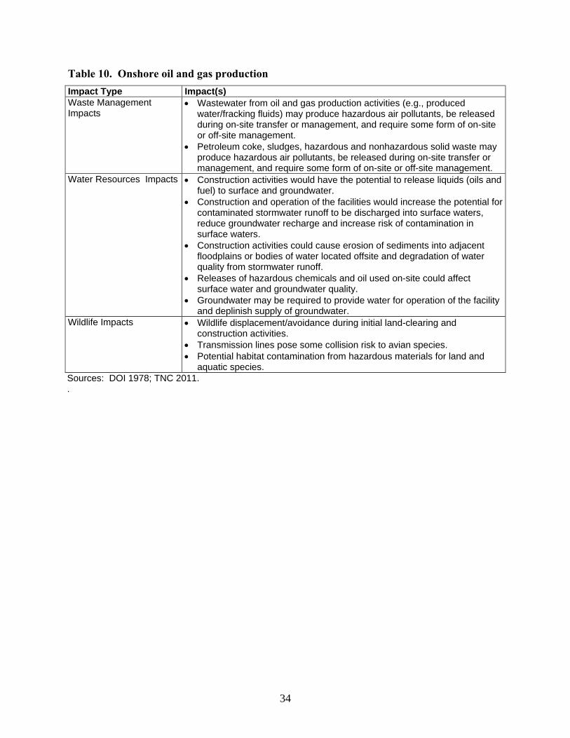
34

Table 10. Onshore oil and gas production


Waste Management Impacts

Wastewater from oil and gas production activities (e.g., produced water/fracking fluids) may produce hazardous air pollutants, be released during on-site transfer or management, and require some form of on-site or off-site management.

Petroleum coke, sludges, hazardous and nonhazardous solid waste may produce hazardous air pollutants, be released during on-site transfer or management, and require some form of on-site or off-site management.

Water Resources Impacts Construction activities would have the potential to release liquids (oils and fuel) to surface and groundwater.

Construction and operation of the facilities would increase the potential for contaminated stormwater runoff to be discharged into surface waters, reduce groundwater recharge and increase risk of contamination in surface waters.

Construction activities could cause erosion of sediments into adjacent floodplains or bodies of water located offsite and degradation of water quality from stormwater runoff.

Releases of hazardous chemicals and oil used on-site could affect surface water and groundwater quality.

Groundwater may be required to provide water for operation of the facility and deplinish supply of groundwater.

Wildlife Impacts Wildlife displacement/avoidance during initial land-clearing and construction activities.

Transmission lines pose some collision risk to avian species.

Potential habitat contamination from hazardous materials for land and aquatic species.

Sources: DOI 1978; TNC 2011. .

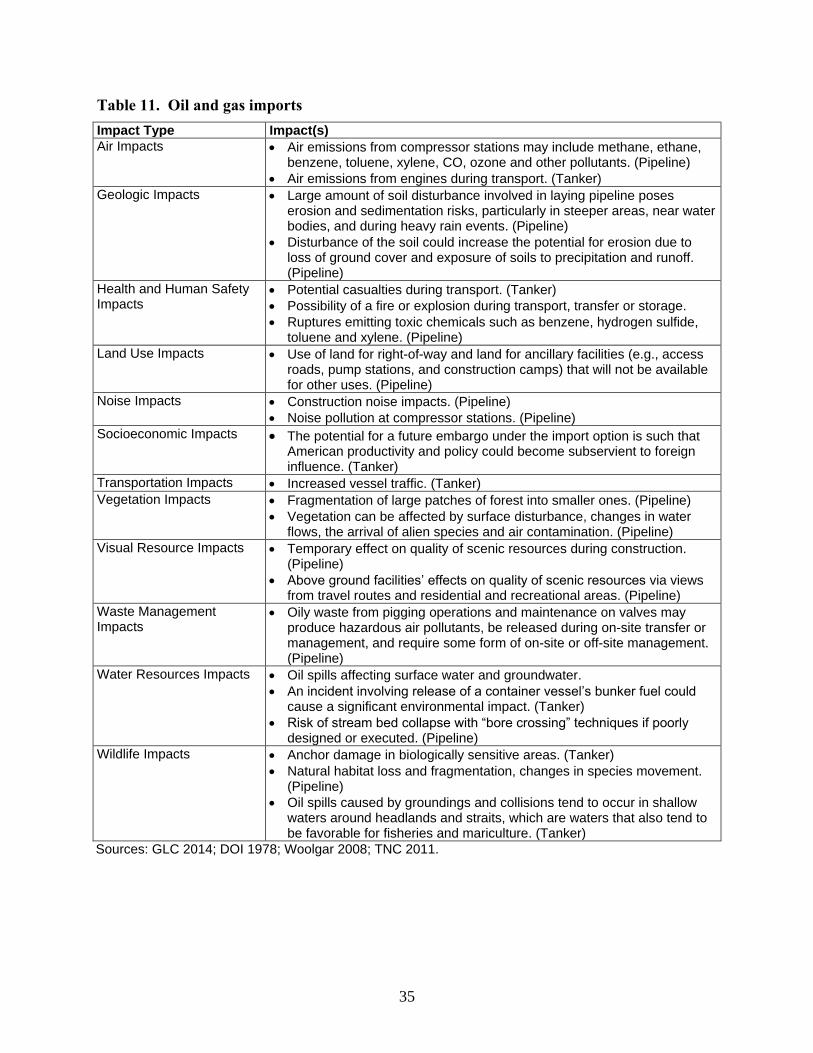
35

Table 11. Oil and gas imports


Air Impacts Air emissions from compressor stations may include methane, ethane, benzene, toluene, xylene, CO, ozone and other pollutants. (Pipeline)

Air emissions from engines during transport. (Tanker)

Geologic Impacts Large amount of soil disturbance involved in laying pipeline poses erosion and sedimentation risks, particularly in steeper areas, near water bodies, and during heavy rain events. (Pipeline)

Disturbance of the soil could increase the potential for erosion due to loss of ground cover and exposure of soils to precipitation and runoff. (Pipeline)


Potential casualties during transport. (Tanker)

Possibility of a fire or explosion during transport, transfer or storage.

Ruptures emitting toxic chemicals such as benzene, hydrogen sulfide, toluene and xylene. (Pipeline)

Land Use Impacts Use of land for right-of-way and land for ancillary facilities (e.g., access roads, pump stations, and construction camps) that will not be available for other uses. (Pipeline)

Noise Impacts Construction noise impacts. (Pipeline)

Noise pollution at compressor stations. (Pipeline)

Socioeconomic Impacts The potential for a future embargo under the import option is such that American productivity and policy could become subservient to foreign influence. (Tanker)

Transportation Impacts Increased vessel traffic. (Tanker)

Vegetation Impacts Fragmentation of large patches of forest into smaller ones. (Pipeline)

Vegetation can be affected by surface disturbance, changes in water flows, the arrival of alien species and air contamination. (Pipeline)

Visual Resource Impacts Temporary effect on quality of scenic resources during construction. (Pipeline)

Above ground facilities’ effects on quality of scenic resources via views from travel routes and residential and recreational areas. (Pipeline)


Oily waste from pigging operations and maintenance on valves may produce hazardous air pollutants, be released during on-site transfer or management, and require some form of on-site or off-site management. (Pipeline)

Water Resources Impacts Oil spills affecting surface water and groundwater.

An incident involving release of a container vessel’s bunker fuel could cause a significant environmental impact. (Tanker)

Risk of stream bed collapse with “bore crossing” techniques if poorly designed or executed. (Pipeline)

Wildlife Impacts Anchor damage in biologically sensitive areas. (Tanker)

Natural habitat loss and fragmentation, changes in species movement. (Pipeline)

Oil spills caused by groundings and collisions tend to occur in shallow waters around headlands and straits, which are waters that also tend to be favorable for fisheries and mariculture. (Tanker)

Sources: GLC 2014; DOI 1978; Woolgar 2008; TNC 2011.

36

Table 12. Coal production


Air Impacts Construction would cause a temporary increase in emissions of CO, NOx, VOCs, and fugitive dust from construction equipment operation.

(Fischer-Tropsch Process) The processing of coal into liquid fuel would result in a minor impact to air quality due to emissions, primarily nitrogen and carbon dioxide.

The gasification process would result in an increase in annual air emissions of NOx, CO, sulfur oxides, particulate matter (PM), VOCs (a precursor of ozone), and reactive organic gases.

(Shell Gasification) Some odors would be emitted during operation of the facilities. Sources for these odors would include diesel engine exhaust from locomotives, trucks, maintenance equipment, and coal yard loaders; the coal pile and coal handling; sulfur storage and handling; and ammonia storage and handling.

(Shell Gasification) Heat Recovery Steam Generator stack emissions include mercury and beryllium.

Carbon dioxide emissions could contribute to local, regional, or global climate change.

Geologic Impacts Impacts to soils as a result of construction activities including grading, paving, and establishing impervious surfaces to support the plant and associated infrastructure.



Potential occupational risks during construction include the movement of heavy objects; slips, trips and falls; the risk of fire or explosion from general construction activities; and spills and exposures related to the storage and handling of chemicals and disposal of hazardous waste.

Potential for injuries and fatalities associated with mining coal.


Hazards associated with possibility of fires, spills/releases of hazardous chemicals.

(Shell Gasification) Short- and long-term inhalation exposure can lead to non-cancerous health impacts, including exposure from manganese, hydrogen chloride, hydrogen fluoride, and acrolein.

Potential impact on quality-of-life issues affecting daily life for asthmatics, such as restricted activity days and days with symptoms.



Vehicle and rail traffic would create noise during facility operations.



Increased employment opportunities to support operations.

Transportation Impacts Construction-related truck traffic.

Increased traffic on roads and highways.

Increased rail traffic.

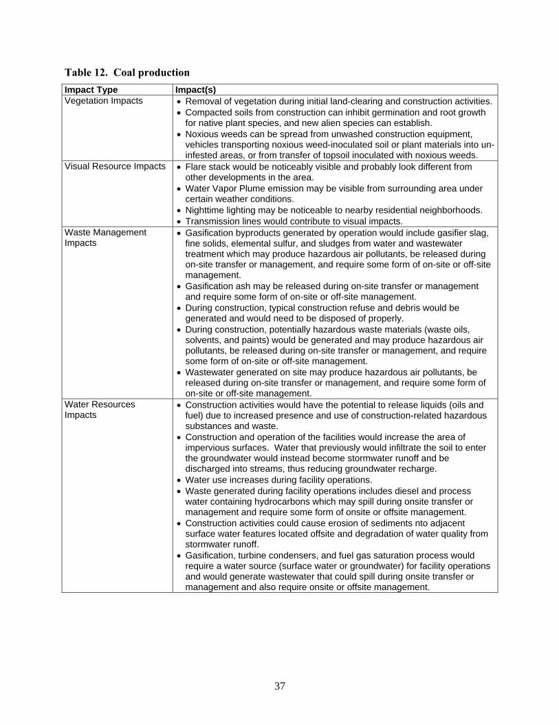
37






Visual Resource Impacts Flare stack would be noticeably visible and probably look different from other developments in the area.

Water Vapor Plume emission may be visible from surrounding area under certain weather conditions.




Gasification byproducts generated by operation would include gasifier slag, fine solids, elemental sulfur, and sludges from water and wastewater treatment which may produce hazardous air pollutants, be released during on-site transfer or management, and require some form of on-site or off-site management.

Gasification ash may be released during on-site transfer or management and require some form of on-site or off-site management.

During construction, typical construction refuse and debris would be generated and would need to be disposed of properly.

During construction, potentially hazardous waste materials (waste oils, solvents, and paints) would be generated and may produce hazardous air pollutants, be released during on-site transfer or management, and require some form of on-site or off-site management.

Wastewater generated on site may produce hazardous air pollutants, be released during on-site transfer or management, and require some form of on-site or off-site management.

Water Resources Impacts

Construction activities would have the potential to release liquids (oils and fuel) due to increased presence and use of construction-related hazardous substances and waste.

Construction and operation of the facilities would increase the area of impervious surfaces. Water that previously would infiltrate the soil to enter the groundwater would instead become stormwater runoff and be discharged into streams, thus reducing groundwater recharge.

Water use increases during facility operations.

Waste generated during facility operations includes diesel and process water containing hydrocarbons which may spill during onsite transfer or management and require some form of onsite or offsite management.

Construction activities could cause erosion of sediments nto adjacent surface water features located offsite and degradation of water quality from stormwater runoff.

Gasification, turbine condensers, and fuel gas saturation process would require a water source (surface water or groundwater) for facility operations and would generate wastewater that could spill during onsite transfer or management and also require onsite or offsite management.

38



Wildlife Impacts Wildlife displacement/avoidance during initial land-clearing and construction.


Operation of the flare would create an altered visual environment at night when the flame would be visible to active wildlife, specifically birds, which could be attracted to the flame.


Source: DOE 2007a.

39

Table 13. Biofuels


Air Impacts The processing of biofuel feedstocks can affect local air quality with CO, particulates, NOx, sulphates, and VOCs released by industrial processes.







Operations involving high temperatures and pressures, as well as flammable/toxic liquids, and the potential for exposure to PM.

Risk of potential spills and exposures to released vapors.

Potential fire hazard due to the storage of large quantities of flammable liquids.


Diversion of farmland use from food supply to biofuel feedstock supply.


During operation, some equipment (such as chippers) may contribute to some additional noise.

Socioeconomic Impacts Potential for land rights disputes as industrial-scale crops are planted to produce biofuel feedstock.

Diversion of farmland use from food supply to biofuel feedstock supply can jeopardize food security and could raise food prices.

Could impact local industry that supports other land uses such as recreation and hunting.

Can impact the nonmarket values of open space.

Transportation Impacts Increase in traffic during construction, as well as increased traffic for facility employees during operation.

Vegetation Impacts Loss of agrobiodiversity induced by intensification on croplands, in the form of crop genetic uniformity.

Low levels of genetic diversity increases the susceptibility of these crops to new pests and diseases.

Visual Resource Impacts Nighttime lighting may be noticeable to nearby residential neighborhoods.

Clearing of land for construction and/or land use changes may lead to temporary aesthetic impacts.


Potential for the production of small quantities of hazardous materials (waste oils, lubricants, solvents, cleaners, paints) during construction which may produce hazardous air pollutants, be released during on-site transfer or management, and require some form of on-site or off-site management.

Char and ash produced during operations may be released during on-site transfer or management and require some form of on-site or off-site management.

40

Table 13. Biofuels


Water Resources Impacts Many of the crops currently used for biofuel production – such as sugar cane, oil palm and maize – have relatively high water requirements at commercial yield levels--the processing of feedstocks into biofuels can use large quantities of water, mainly for washing plants and seeds and for evaporative cooling.

Irrigated production of the key biofuel feedstocks have the greatest impact on local water resource balances.

Converting pastures or woodlands into maize fields (example) may exacerbate problems such as soil erosion, sedimentation and excess nutrient (nitrogen and phosphorus) runoff into surface waters and infiltration into groundwater.

Excess nitrogen into water pathways causing “dead zones.”

Pesticides and other chemicals can wash into waterbodies, negatively affecting water quality.

Wildlife Impacts Biodiversity loss following land conversion and habitat loss.

Agricultural expansion driven by higher prices could endanger areas rich in bird species diversity.

Sources: DOE 2007b; FAO 2008; German et al. 2011.

41

Table 14. Biomass


Air Impacts Construction, harvesting and transportation would generate emissions and dust from operation of equipment.

Biomass project’s power plant/wood boiler/biorefinery uses fuel and generates greenhouse gases, primarily carbon dioxide, methane, nitrous oxide and a small amount of sulfur dioxide (SO2).




The harvesting of biomass can result in short-term disturbances to and modifications of soil structure.






Socioeconomic Impacts




Transportation Impacts

Increase in traffic during construction, as well as increased traffic for facility employees during operation.




Visual Resource Impacts




Potential for the production of small quantities of hazardous materials (waste oils, lubricants, solvents, cleaners, paints) during construction that may produce hazardous air pollutants, be released during on-site transfer or management, and require some form of on-site or off-site management.

Ash produced during operations may be released during on-site transfer or management and require some form of on-site or off-site management.


General construction impacts could affect water resources by increased stormwater runoff being generated from the construction locations which could carry sediment and contamination loads into vicinity surface waters during times of heavy rain, and contamination from construction activities infiltrating area soils and percolating down into the groundwater.

Increased stormwater runoff occurs from developed sites as vegetation is removed and as the amount of impervious surface area increases, posing a risk of contaminating water and harming aquatic life.

Reduction of groundwater levels due to the irrigation demand of biomass crops prior to harvesting.

42

Table 14. Biomass


Wildlife Impacts During (woody) biomass harvest, change in successional stage and forest structure impact wildlife species differently. Late successional stage species such as birds that nest in mature forests would be negatively impacted following the first harvest, and early successional stage species such as mammals that live and feed on young forest stages would be positively impacted.

New transmission lines could increase potential hazards to birds such as collision or electrocution.

Noise from biomass harvesting activities could temporarily affect wildlife.

Source: DOE 2011a.

43

Table 15. Geothermal



Emissions associated with generating electricity from geothermal technologies are negligible because no fuels are combusted.






Exposure of individuals to drilling mud and geothermal fluid or steam during exploration and development (E&D) drilling activities.

Exposure of individuals to hydrogen sulfide contained in geothermal fluid or steam during exploration, development, and operation phases.

Exposure of individuals to hazardous materials used and stored at facilities, such as petroleum oil, lubricants, paints, solvents and herbicides.

Land Use Impacts Could remove farmland or forestland from production.

If water is not re-injected into the ground after use to maintain pressure underground, it may cause sinking of land at the surface.


Areas with minimal noise sources (remote areas) would experience a greater change in the noise characteristics.






Transportation Impacts Increased traffic on nearby roads during construction.

Increased traffic for facility employees during operation.








Solid waste and hazardous waste (paints, coatings, solvents) generated during construction may produce hazardous air pollutants, be released during on-site transfer or management, and require some form of on-site or off-site management.

44

Table 15. Geothermal



Potential for groundwater contamination when drilling wells and extracting hot water or steam (can be prevented with proper management techniques).

Wildlife Impacts Loss of wildlife habitat from the surface disturbance required for construction of drilling pads and access roads.

Project generated noise could keep some animals away from areas directly affected by surface disturbance during the on-site project construction and drilling activities.

Source: TEEIC 2015.

45

Table 16. Hydroelectric


Air Impacts Construction would cause a temporary increase in emissions of CO, NOx, VOCs, and fugitive dust from construction equipment operation. If a large amount of vegetation is growing along the riverbed when a dam is built, it can decay in the lake that is created, causing the buildup and release of methane, a greenhouse gas.


Potential for slope failures, landslides, and rock falls during construction where construction involves earth moving.

Erosion of shoreline and sediment transport.

Reservoir-triggered seismicity (where the chance exists).

Changes in channel morphology and bed surface texture in the bypassed and peaking reaches from changes in project operations affecting supply and transport of sediment.




Land Use Impacts The construction of hydropower plants can alter sizable portions of land when dams are constructed and lakes are created, flooding land that may have once served as wildlife habitat, farmland, and scenic retreat.


Socioeconomic Impacts Potential for gain or loss of water-based recreation and fisheries.

Displacement of residents for construction of the dam and creation of water body.





Colonization of invasive plant species due to the fluctuating water levels in the reservoirs.

Visual Resource Impacts Transmission lines would contribute to visual impacts.


Possible positive or negative visual effects due to lake creation, depending on setting.


Some material may need to be dredged from reservoirs and disposed of properly.

Hazardous and nonhazardous wastes related to maintenance activities may produce hazardous air pollutants, be released during on-site transfer or management, and require some form of on-site or off-site management.

46

Table 16. Hydroelectric



Construction may cause the change of surface water flow patterns and increase erosion and sedimentation.

In cases where cofferdams are being used during construction, future erosion may result in the release of lower oxygenated water downstream.

If wells are emptied in order to fill reservoirs, groundwater levels would be affected by construction of reservoir. After the reservoirs are filled, high evaporation rates could degrade the water quality in the reservoirs and seepage from the reservoirs could affect nearby groundwater quality.

Fluctuation of water levels in the reservoirs could have an impact on acid production from water interaction with the rocks surrounding the reservoirs.

Discharge of pollutants (e.g., fuels, lubricants, and other hazardous materials) and other contaminants (e.g., human waste and petroleum products) into adjacent rivers, streams, and reservoirs and groundwater; and contamination of water supply systems.

Wildlife Impacts Filling the reservoirs and creating a new source of drinking water for wildlife has the potential to alter migration movement for some species and disturb wildlife habitat.

Hydroelectric power plants affect various fish populations in different ways.

Construction activities will create adverse impacts for wildlife, and will create hazardous areas for local wildlife, including open pits, material stockpiles, shade created by equipment, and clearing of vegetation.

Birds are likely to view the ponds as a safe source of drinking water or resting area. However, high total dissolved solids concentrations in these proposed ponds could be harmful or fatal to birds and other wildlife.

New transmission lines could increase potential hazards to birds such as collision or electrocution.

Source: ORNL et al. 2010.

47

Table 17. Municipal waste


Air Impacts Emissions of fugitive dust and exhaust from vehicles and equipment during construction and increased emissions of criteria pollutants, formaldehyde, and acetaldehyde during operations.

During the operation phase the main sources of pollution should be the boiler stack emissions, emissions from refuse-derived fuel (RDF) plant, and fugitive dust and odor emissions from waste handling and processing emissions due to vehicular movement.

Possible air pollutants released during operations include PM, VOCs, CO, SO2, NOx, formaldehyde and acetaldehyde.









Increased truck traffic may cause higher noise levels.

Noise emissions from equipment such as shredders, boilers, generators, etc.


Potential adverse impacts to desirability of real estate and decreased property values in the surrounding area.










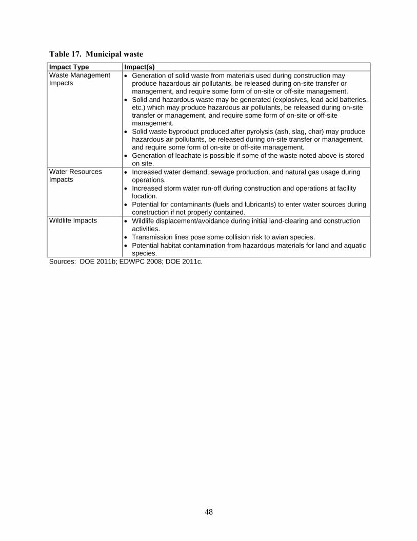
48

Table 17. Municipal waste



Generation of solid waste from materials used during construction may produce hazardous air pollutants, be released during on-site transfer or management, and require some form of on-site or off-site management.

Solid and hazardous waste may be generated (explosives, lead acid batteries, etc.) which may produce hazardous air pollutants, be released during on-site transfer or management, and require some form of on-site or off-site management.

Solid waste byproduct produced after pyrolysis (ash, slag, char) may produce hazardous air pollutants, be released during on-site transfer or management, and require some form of on-site or off-site management.

Generation of leachate is possible if some of the waste noted above is stored on site.


Increased water demand, sewage production, and natural gas usage during operations.

Increased storm water run-off during construction and operations at facility location.

Potential for contaminants (fuels and lubricants) to enter water sources during construction if not properly contained.




Sources: DOE 2011b; EDWPC 2008; DOE 2011c.

49

Table 18. Nuclear



During operation, releases to the environment of heat and moisture from the primary cooling system, operation of auxiliary equipment (generators and boilers), and emissions from workers’ vehicles would be the primary impacts to air quality.

No greenhouse gases emitted related to the direct generation of electricity.






Public and workers would be exposed to increased ambient background radiation.



Some impact to ambient background noise.


Potential adverse impacts to desirability of real estate and decreased property values in the surrounding area.




Increase in traffic during construction, as well as increased traffic for facility employees during operation.




The thermal plume discharged into the water source, along with chemical and physical impacts, may have a negative impact on the aquatic ecosystem for nuclear plants that use water bodies as a heat sink.

Biota would be exposed to increased ambient background radiation.




Cooling towers and their associated vapor plumes would be clearly visible to nearby residents.

50

Table 18. Nuclear



During construction, typical construction refuse and debris, hazardous and nonhazardous wastes, are generated that may produce hazardous air pollutants, be released during on-site transfer or management, and require some form of on-site or off-site management.

During operation, waste management would involve the following, which will require on-site and off-site management: o Transuranic waste o Low-level radioactive waste o Mixed low-level radioactive waste o Chemical waste o Solid waste o Sanitary wastewater o Liquid low-level radioactive waste


Construction activities would have the potential to release liquids (oils and fuel) due to increased presence and use of construction-related hazardous substances and waste.

Construction and operation of the facilities would increase the area of impervious surfaces. Water that previously would infiltrate the soil to enter the groundwater would instead become stormwater runoff and be discharged into streams, thus reducing groundwater recharge.

Construction activities could cause erosion of sediments into adjacent surface water features located offsite and degradation of water quality from stormwater runoff.

Groundwater and/or surface water would be withdrawn to provided water needed for operation of the facility (if withdrawing from surface water, impact would fluctuate with water levels) o The groundwater withdrawal can have a potential offsite impact of that

water not being available to other users o Also, neighboring groundwater users may experience higher pumping

costs due to the physical drawdown of the hydraulic head of the confined aquifer


Noise impacts during operation may lead to habitat loss through avoidance, reduced reproductive success, and mortality.

The thermal plume discharged into the water source may have a negative impact on the aquatic ecosystem.

The chemical and physical impacts from the water discharge into the water source may have a negative impact on the aquatic ecosystem.

Biota would be exposed to increased ambient background radiation from a nuclear unit.


Source: WNA 2013.

51

Table 19. Other natural gas


Air Impacts Synthetic natural gas (SNG) plants can be major point sources of emissions

of sulfur compounds (primarily SO2) and hydrocarbons, and to a lesser extent, of CO, NOx and particulates.


Geologic Impacts Impacts to soil as a result of construction activities including grading, paving, and establishing impervious surfaces to support the plant and associated infrastructure.





Exposure to gaseous and particulate emissions.



Some impact to ambient background noise.











Hazardous and nonhazardous wastes from construction and operations may produce hazardous air pollutants, be released during on-site transfer or management, and require some form of on-site or off-site management.


May have indirect impacts on the quality of the surface waters and ground waters due to extensive water withdrawals, possible intermedia transfer of pollutants or accidents and system failures.

The intermedia pollution transfer routes may include percolation of wastewaters from impoundments and leachates from landfill/mines, uncontrolled runoff from plant sites and precipitation of air pollutants from the facility.


Natural habitat loss and fragmentation, changes in species movement.


Source: EPA 1979.

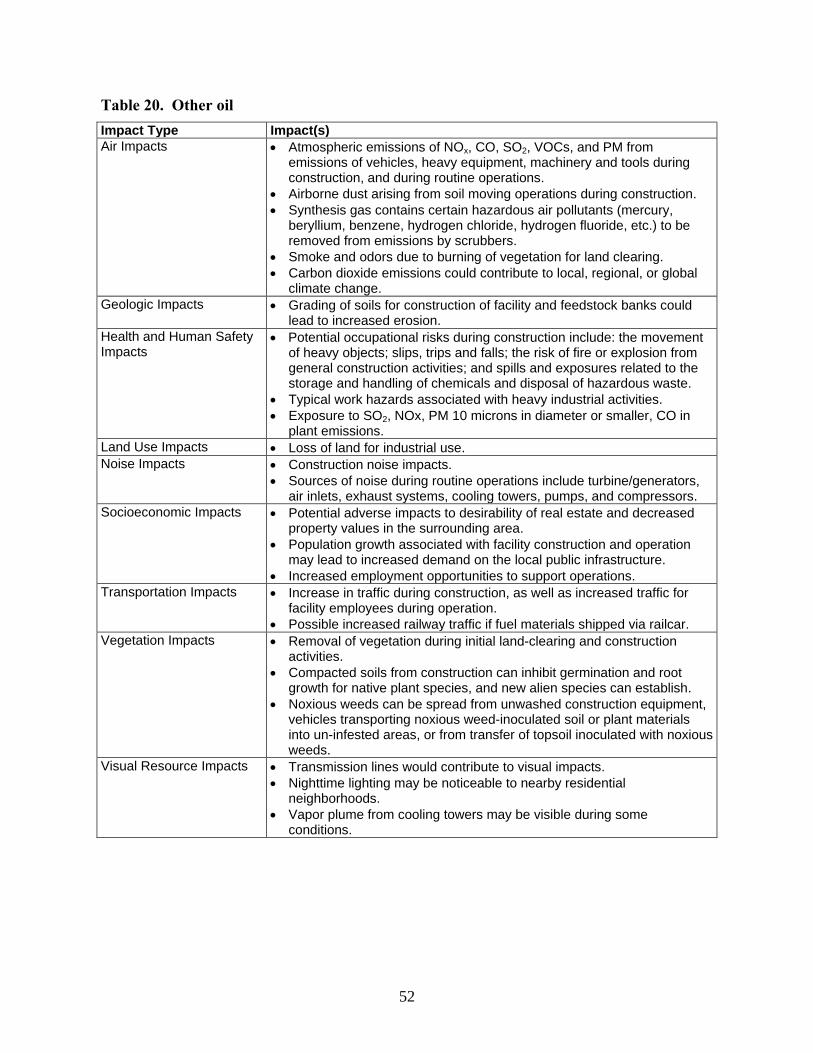
52

Table 20. Other oil


Air Impacts Atmospheric emissions of NOx, CO, SO2, VOCs, and PM from emissions of vehicles, heavy equipment, machinery and tools during construction, and during routine operations.

Airborne dust arising from soil moving operations during construction.

Synthesis gas contains certain hazardous air pollutants (mercury, beryllium, benzene, hydrogen chloride, hydrogen fluoride, etc.) to be removed from emissions by scrubbers.

Smoke and odors due to burning of vegetation for land clearing.


Geologic Impacts Grading of soils for construction of facility and feedstock banks could lead to increased erosion.




Exposure to SO2, NOx, PM 10 microns in diameter or smaller, CO in plant emissions.



Sources of noise during routine operations include turbine/generators, air inlets, exhaust systems, cooling towers, pumps, and compressors.





Possible increased railway traffic if fuel materials shipped via railcar.






Vapor plume from cooling towers may be visible during some conditions.

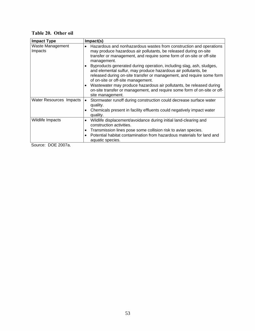
53

Table 20. Other oil



Hazardous and nonhazardous wastes from construction and operations may produce hazardous air pollutants, be released during on-site transfer or management, and require some form of on-site or off-site management.

Byproducts generated during operation, including slag, ash, sludges, and elemental sulfur, may produce hazardous air pollutants, be released during on-site transfer or management, and require some form of on-site or off-site management.

Wastewater may produce hazardous air pollutants, be released during on-site transfer or management, and require some form of on-site or off-site management.

Water Resources Impacts Stormwater runoff during construction could decrease surface water quality.

Chemicals present in facility effluents could negatively impact water quality.




Source: DOE 2007a.

54

Table 21. Solar








Increased number of traffic accidents or retinal damage due to glare from equipment associated with solar developments.



Equipment, motor vehicles, high pressure steam blow.




Visibility of solar developments from recreational areas could reduce visitation and tourism in the area.

Transportation Impacts Increase in traffic during construction.

Glare from the solar receivers can impact nearby roadways.

Vegetation Impacts Solar development will typically require the total removal of vegetation at most facilities, increasing the risk of invasive species introduction, changes in species composition and distribution, habitat loss (e.g., dune or riparian areas), and damage to biological soil crusts.

Indirect impacts also likely in terms of dust deposition, altered drainage patterns, runoff, and sedimentation.

Visual Resource Impacts Solar development would alter the character of largely rural areas along with development of supporting infrastructure.



Hazardous wastes similar to those generated during construction of other industrial facilities (cleaners, paints, fuels, etc.) and nonhazardous wastes during construction of solar energy facility that could be released during on-site management and will also require on-site and off-site management.

Hazardous materials required for routine maintenance of solar components and equipment: o May include water treatment needs for washing fluids o May include dielectric fluids


Solar thermal projects with wet-cooling systems require large volumes of water. Solar thermal projects with dry-cooling systems need less than one-tenth of the amount of water required for wet-cooling systems.

Modification of surface and groundwater flow systems.

Water contamination resulting from chemical leaks or spills.

Water quality degradation by runoff or excessive withdrawals.

55

Table 21. Solar


Wildlife Impacts Loss of habitat, disturbance, loss of food and prey species, loss of breeding areas, effects on movement and migration, introduction of new species, habitat fragmentation, and changes in water availability.

Operation of the project may result in bird collisions with the heliostat mirrors and incineration at or near focused solar heat at the central tower.

Construction would have the potential to interrupt wildlife movement through the area.

Sources: DOE 2010a; DOE 2012a.

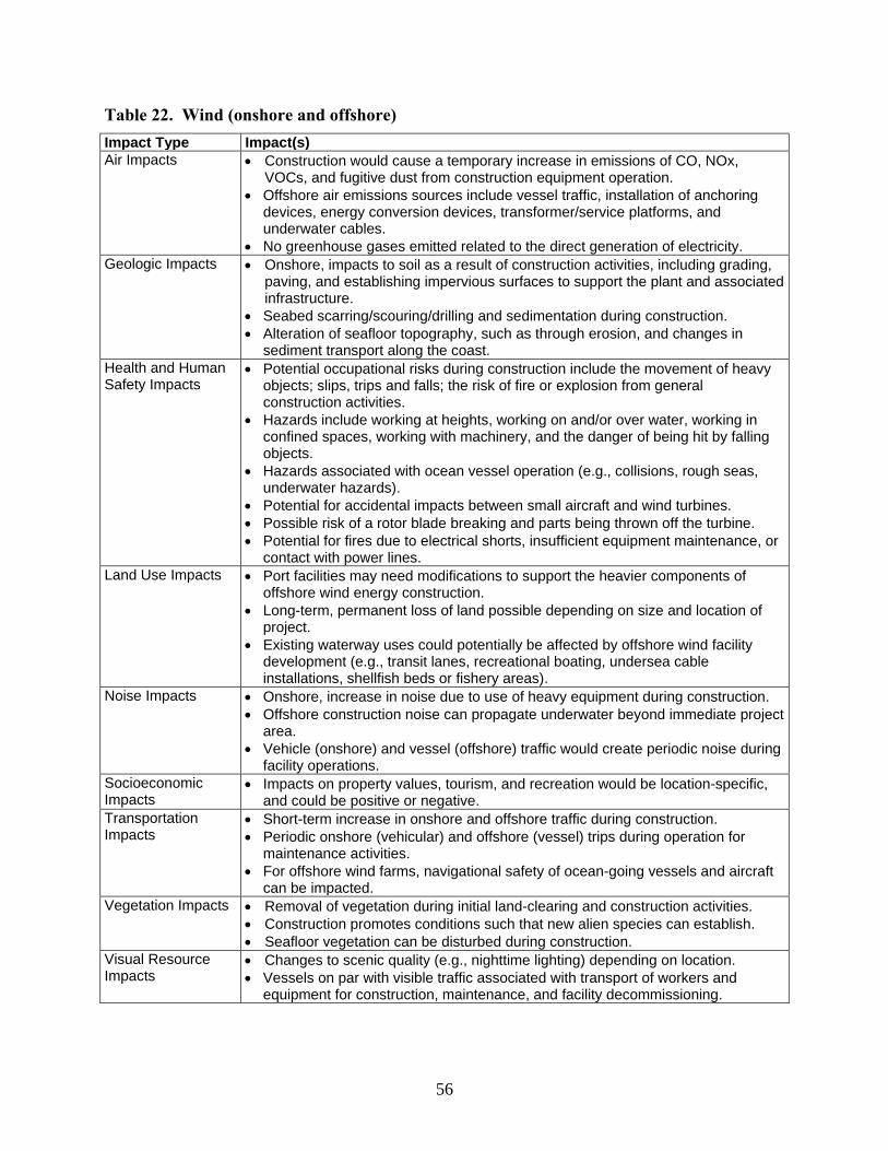
56

Table 22. Wind (onshore and offshore)



Offshore air emissions sources include vessel traffic, installation of anchoring devices, energy conversion devices, transformer/service platforms, and underwater cables.


Geologic Impacts Onshore, impacts to soil as a result of construction activities, including grading, paving, and establishing impervious surfaces to support the plant and associated infrastructure.

Seabed scarring/scouring/drilling and sedimentation during construction.

Alteration of seafloor topography, such as through erosion, and changes in sediment transport along the coast.


Potential occupational risks during construction include the movement of heavy objects; slips, trips and falls; the risk of fire or explosion from general construction activities.

Hazards include working at heights, working on and/or over water, working in confined spaces, working with machinery, and the danger of being hit by falling objects.

Hazards associated with ocean vessel operation (e.g., collisions, rough seas, underwater hazards).

Potential for accidental impacts between small aircraft and wind turbines.

Possible risk of a rotor blade breaking and parts being thrown off the turbine.

Potential for fires due to electrical shorts, insufficient equipment maintenance, or contact with power lines.

Land Use Impacts Port facilities may need modifications to support the heavier components of offshore wind energy construction.

Long-term, permanent loss of land possible depending on size and location of project.

Existing waterway uses could potentially be affected by offshore wind facility development (e.g., transit lanes, recreational boating, undersea cable installations, shellfish beds or fishery areas).

Noise Impacts Onshore, increase in noise due to use of heavy equipment during construction.

Offshore construction noise can propagate underwater beyond immediate project area.

Vehicle (onshore) and vessel (offshore) traffic would create periodic noise during facility operations.


Impacts on property values, tourism, and recreation would be location-specific, and could be positive or negative.


Short-term increase in onshore and offshore traffic during construction.

Periodic onshore (vehicular) and offshore (vessel) trips during operation for maintenance activities.

For offshore wind farms, navigational safety of ocean-going vessels and aircraft can be impacted.


Construction promotes conditions such that new alien species can establish.

Seafloor vegetation can be disturbed during construction.


Changes to scenic quality (e.g., nighttime lighting) depending on location.

Vessels on par with visible traffic associated with transport of workers and equipment for construction, maintenance, and facility decommissioning.

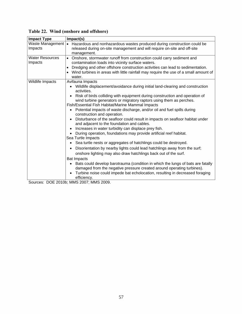
57

Table 22. Wind (onshore and offshore)



Hazardous and nonhazardous wastes produced during construction could be released during on-site management and will require on-site and off-site management.


Onshore, stormwater runoff from construction could carry sediment and contamination loads into vicinity surface waters.

Dredging and other offshore construction activities can lead to sedimentation.

Wind turbines in areas with little rainfall may require the use of a small amount of water.

Wildlife Impacts Avifauna Impacts

Wildlife displacement/avoidance during initial land-clearing and construction activities.

Risk of birds colliding with equipment during construction and operation of wind turbine generators or migratory raptors using them as perches.

Fish/Essential Fish Habitat/Marine Mammal Impacts

Potential impacts of waste discharge, and/or oil and fuel spills during construction and operation.

Disturbance of the seafloor could result in impacts on seafloor habitat under and adjacent to the foundation and cables.

Increases in water turbidity can displace prey fish.

During operation, foundations may provide artificial reef habitat. Sea Turtle Impacts

Sea turtle nests or aggregates of hatchlings could be destroyed.

Disorientation by nearby lights could lead hatchlings away from the surf;

onshore lighting may also draw hatchlings back out of the surf.

Bat Impacts

Bats could develop barotrauma (condition in which the lungs of bats are fatally damaged from the negative pressure created around operating turbines).

Turbine noise could impede bat echolocation, resulting in decreased foraging efficiency.

Sources: DOE 2010b; MMS 2007; MMS 2009.

58

2.4 REFERENCES

ARC/USDA 2010. “Appalachian Regional Development Initiative Listening Session and Online

Outreach Report,” U.S. Department of Agriculture (USDA), the Appalachian Regional

Commission (ARC). May 27, 2010. Available online at:

http://www.arc.gov/noindex/programs/ardi/ARDIOutreachReport.PDF

Davis 2010. “The Effect of Power Plants on Local Housing Values and Rents,” Author Lucas

W. Davis, Haas School of Business, University of California, Berkeley, California, and

National Bureau of Economic Research. May 2010. Available online at:

http://faculty.haas.berkeley.edu/ldavis/pp.pdf

DESMOG 2013. “Over 865,200 Gallons of Fracked Oil Spill in ND, Public in Dark for Days

due to Government Shutdown.” Article posted on the DESMOG, Clearing the PR

Pollution that Clouds Climate Science web site. October 13, 2013. Available at:

http://www.desmogblog.com/2013/10/10/20600-barrels-fracked-oil-spill-north-dakota-

publicity-halted-due-government-shutdown

DOE 1978. “EIS-0002: Final Environmental Impact Statement: Allocation of Petroleum

Feedstock, Baltimore Gas and Electric Company, Sollers Point SNG Plant, Sollers Point,

Baltimore County, Maryland,” U.S. Department of Energy, April 1978.

DOE 2007a. “EIS-0357: Final Environmental Impact Statement for the Gilberton Coal-To-

Clean Fuels and Power Project, Gilberton, Pennsylvania, Volume 1: Main Text,” U.S.

Department of Energy, October 2007.

DOE 2007b. “EA-1597: Final Environmental Assessment: Construction and Operation of a

Proposed Cellulosic Ethanol Plant, Range Fuels, Inc., Treutlen County, Georgia,” U.S.

Department of Energy, October 2007.

DOE 2010a. “EIS-0403, Draft Programmatic Environmental Impact Statement for Solar Energy

Development in Six Southwestern States, Volume 1,” U.S. Department of Energy,

December 2010.

DOE 2010b. “EIS-0418, Final Environmental Impact Statement for the South Dakota

PrairieWinds Project,” U.S. Department of Energy, July 2010.

DOE 2011a. “EA-1858, Final Environmental Assessment for Nippon Paper Industries USA

Company Biomass Cogeneration Project, Port Angeles, Washington,” U.S. Department

of Energy, June 2011.

DOE 2011b. “EA-1862, Final Environmental Assessment for the Oneida Seven Generations

Corporation: Energy Recovery Project, Green Bay, Wisconsin,” U.S. Department of

Energy, November 2011.

http://www.arc.gov/noindex/programs/ardi/ARDIOutreachReport.PDF

http://faculty.haas.berkeley.edu/ldavis/pp.pdf

http://www.desmogblog.com/2013/10/10/20600-barrels-fracked-oil-spill-north-dakota-publicity-halted-due-government-shutdown

http://www.desmogblog.com/2013/10/10/20600-barrels-fracked-oil-spill-north-dakota-publicity-halted-due-government-shutdown

59

DOE 2011c. “DOE/EA-1860, Draft Environmental Assessment for the Richland Center

Renewable Energy Anaerobic Digester-Waste to Energy Project,” U.S. Department of

Energy, Golden Field Office. August 2011. Accessed in April 2015 at

energy.gov/sites/prod/files/EA-1860-DEA-2011.pdf

DOE 2012a. “EIS-0403, Final Programmatic Environmental Impact Statement for Solar Energy

Development in Six Southwestern States, Volume 1,” U.S. Department of Energy, July

2012.

DOE 2012b. Choosing and Installing Geothermal Heat Pumps, “Benefits of Geothermal Heat

Pump Systems,” June 24, 2012. Available online at:

http://energy.gov/energysaver/articles/choosing-and-installing-geothermal-heat-pumps.

DOE 2015a. “Buildings Energy Data Book,” U.S. Department of Energy, Energy Efficiency and

Renewable Energy, 2015; Table 2.1.6, 2015 Residential Energy End-Use Splits, by Fuel

Type (Quadrillion Btu), accessed online at:

http://buildingsdatabook.eren.doe.gov/TableView.aspx?table=2.1.6

DOE 2015b. “Buildings Energy Data Book,” U.S. Department of Energy, Energy Efficiency and

Renewable Energy, 2015; Table 3.1.5, 2015 Commercial Energy End-Use Splits, by Fuel

Type (Quadrillion Btu), accessed online at:


DOI 1978. “Draft Environmental Impact Statement: Proposed 1979 OCS Oil and Gas Lease

Sale 58” Department of the Interior, Bureau of Land Management, Published by the

University of Michigan, 1978.

DOL 2015. “Coal Fatalities for 1990 through 2014.” U.S. Department of Labor, Mine Safety

and Health Administration. Date unknown. Available online at:

http://www.msha.gov/stats/centurystats/coalstats.asp

EDWPC 2008. “Environmental Impact Statement of Integrated Municipal Solid Waste

Processing Complex – Ghazipur, Delhi,” Submitted to Delhi Pollution Control

Committee by East Delhi Waste Processing Company Pvt. Ltd. January 2008. Accessed

in April 2015 at: wtert.in/wp-content/uploads/2013/03/gdpcc.pdf

EIA 2013. “Annual Energy Outlook 2013 with projections to 2040,” U.S. Energy Information

Administration, DOE/EIA-0383(2013). April 2013. This publication is on the web at:

http://www.eia.gov/forecasts/aeo/pdf/0383(2013).pdf.

EIA 2015. “Annual Energy Outlook 2015 with projections to 2040,” U.S. Energy Information

Administration, DOE/EIA-0383(2015). April 2015. This publication is on the web at:

http://www.eia.gov/forecasts/aeo/pdf/0383(2015).pdf.

EPA 1979. “Environmental Assessment Report: Lurgi Coal Gasification Systems for SNG,”

EPA-600/7-79-120. U.S. Environmental Protection Agency, Research Triangle Park,

http://energy.gov/energysaver/articles/choosing-and-installing-geothermal-heat-pumps



http://www.msha.gov/stats/centurystats/coalstats.asp

http://www.eia.gov/forecasts/aeo/pdf/0383(2013).pdf

http://www.eia.gov/forecasts/aeo/pdf/0383(2015).pdf

60

North Carolina. May 1979. Available at http://nepis.epa.gov, search on the document

number.

EPA 2015a. Landfill Methane Outreach Program. Retrieved from U.S. Environmental

Protection Agency at http://www.epa.gov/lmop/basic-info/index.html#a03.

EPA 2015b. Map of operational and under–construction projects and candidate and other

landfills, current as of March 2015 retrieved from U.S. Environmental Protection Agency

at: http://www.epa.gov/lmop/projects-candidates/index.html#map-area

EPA 2015c. “Assessment of the Potential Impacts of Hydraulic Fracturing for Oil and Gas on

Drinking Water Resources (External Review Draft),” U.S. Environmental Protection

Agency. Draft report for public comment, June 4, 2015. Available online at:

http://cfpub.epa.gov/ncea/hfstudy/recordisplay.cfm?deid=244651.

Erickson, W.P., M. Wolfe, K.J. Bay, et al., 2014. “A Comprehensive Analysis of Small-

Passerine Fatalities from Collision with Turbines at Wind Energy Facilities.” PLoS ONE

9:e107491;http://www.plosone.org/article/info%3Adoi%2F10.1371%2Fjournal.pone.010

7491

FAO 2008. Biofuels: Prospects, Risks and Opportunities, “Section 5: Environmental Impacts of

Biofuels,” Article from the Food and Agriculture Organization of the United Nations

headquartered in Rome. Excerpted Section 5 accessed in April 2015 at:

ftp://ftp.fao.org/docrep/fao/011/i0100e/i0100e05.pdf

Flannery, T., and F. Stanley, 2014. “We must kill dirty coal before it kills us,” Article posted on

The Age, an Australian news web site, September 3, 2014. Available at:

http://www.theage.com.au/comment/we-must-kill-dirty-coal-before-it-kills-us-20140902-

10b8lk.html

German, L., Schoneveld, G.C., and Pacheco, P., 2011. “The Social and Environmental Impacts

of Biofuel Feedstock Cultivation: Evidence from Multi-Site Research in the Forest

Frontier,” Ecology and Society, 16(3):24, 2011.

GF 2015. “Liquid Biofuels for Transport Prospects,” GreenFacts. Available online at:

http://www.greenfacts.org/en/biofuels/l-3/4-environmental-impacts.htm

GLC 2014. “Advantages, Disadvantages and Economic Benefits Associated with Crude Oil

Transportation,” Issue Brief 2, Discussion Draft, Great Lakes Commission.

September 19, 2014. https://www.glc.org/oiltransport/files/14-09-19-IssueBrief2-

Discussion-Draft.pdf.

HP 2015. “One Year After Dan River Coal Ash Spill, Regulators Work To Determine Fines

Against Duke Energy,” article by Michael Biesecker and Mitch Weiss in the Huffington

Post. Posted online February 1, 2015; updated April 4, 2015. Available online at:

http://www.huffingtonpost.com/2015/02/02/dan-river-coal-ash-spill_n_6589556.html

http://nepis.epa.gov/

http://www.epa.gov/lmop/basic-info/index.html#a03

http://www.epa.gov/lmop/projects-candidates/index.html#map-area

http://cfpub.epa.gov/ncea/hfstudy/recordisplay.cfm?deid=244651

http://www.plosone.org/article/info%3Adoi%2F10.1371%2Fjournal.pone.0107491

http://www.plosone.org/article/info%3Adoi%2F10.1371%2Fjournal.pone.0107491

ftp://ftp.fao.org/docrep/fao/011/i0100e/i0100e05.pdf

http://www.theage.com.au/comment/we-must-kill-dirty-coal-before-it-kills-us-20140902-10b8lk.html

http://www.theage.com.au/comment/we-must-kill-dirty-coal-before-it-kills-us-20140902-10b8lk.html

http://www.greenfacts.org/en/biofuels/l-3/4-environmental-impacts.htm

https://www.glc.org/oiltransport/files/14-09-19-IssueBrief2-Discussion-Draft.pdf

https://www.glc.org/oiltransport/files/14-09-19-IssueBrief2-Discussion-Draft.pdf

http://www.huffingtonpost.com/2015/02/02/dan-river-coal-ash-spill_n_6589556.html

61

Industrial Economics, Inc. 2015. Consumer Surplus and Energy Substitutes for OCS Oil and

Gas Production: The 2015 Revised Market Simulation Model (MarketSim). U.S.

Department of the Interior, Bureau of Ocean Energy Management. OCS Study BOEM

2015-054.

IRENA 2015. “Renewable Energy Prospects: United States of America, REmap 2030 analysis,”

International Renewable Energy Agency, accessed from: www.irena.org/remap. January

2015.

Loss, S.R., T. Will, and P.P. Marra, 2013. “Estimates of Bird Collision Mortality at Wind

Facilities in the Contiguous United States.” Biol Conserv 168: 201-

09.(http://www.sciencedirect.com/science/article/pii/S0006320713003522)

MMS 2007. Programmatic Environmental Impact Statement for Alternative Energy

Development and Production and Alternative Use of Facilities on the Outer Continental

Shelf, OCS EIS/EA, MMS 2007-046. Volume II: Chapter 5, “Potential Impacts of

Alternative Energy Development on the OCS and Analysis of Potential Mitigation

Measures.”. U.S. Department of the Interior, Minerals Management Service. October

2007. Available online at http://www.boem.gov/Renewable-Energy-

Program/Regulatory-Information/Alt_Energy_FPEIS_Chapter5.aspx.

MMS 2009. Cape Wind Energy Project, Final Environmental Impact Statement, MMS EIS-EA,

OCS Publication No. 2008-040. Chapter 4, “Description of Affected Environment.”

U.S. Department of the Interior, Minerals Management Service. January 2009.

Available online at http://www.boem.gov/Renewable-Energy-

Program/Studies/FEIS/Section4-0AffectedEnvironment.aspx.

NRC 2015. “Combined License Applications for New Reactors.” U.S. Nuclear Regulatory

Commission. Page Last Reviewed/Updated Monday, May 18, 2015.

http://www.nrc.gov/reactors/new-reactors/col.html

NRDC 2014. “Fracking Fumes: Air Pollution from Hydraulic Fracturing Threatens Public

Health and Communities,” NRDC Issue Brief, IP:14-10-A. Tanja Srebotnjak and Miriam

Rotkin-Ellman, Natural Resources Defense Council. December 2014. Available online

at: http://www.nrdc.org/health/files/fracking-air-pollution-IB.pdf

NREL no date. National Renewable Energy Laboratory web site, Dynamic Maps, GIS Data, &

Analysis Tools, creation date unknown. Accessed June 2015 at:

http://www.nrel.gov/gis/mhk.html

NREL 2009. National Renewable Energy Laboratory web site, Dynamic Maps, GIS Data, &

Analysis Tools, Map created October 13, 2009. Accessed June 2015 at:

http://nrel.gov/gis/images/geothermal_resource2009-final.jpg

http://www.irena.org/remap

http://www.sciencedirect.com/science/article/pii/S0006320713003522

http://www.boem.gov/Renewable-Energy-Program/Regulatory-Information/Alt_Energy_FPEIS_Chapter5.aspx

http://www.boem.gov/Renewable-Energy-Program/Regulatory-Information/Alt_Energy_FPEIS_Chapter5.aspx

http://www.boem.gov/Renewable-Energy-Program/Studies/FEIS/Section4-0AffectedEnvironment.aspx

http://www.boem.gov/Renewable-Energy-Program/Studies/FEIS/Section4-0AffectedEnvironment.aspx

http://www.nrc.gov/reactors/new-reactors/col.html

http://www.nrdc.org/health/files/fracking-air-pollution-IB.pdf

http://www.nrel.gov/gis/mhk.html

http://nrel.gov/gis/images/geothermal_resource2009-final.jpg

62

NREL 2011. National Renewable Energy Laboratory web site, Dynamic Maps, GIS Data, &

Analysis Tools, Map created April 1, 2011. Accessed June 2015 at:

http://www.nrel.gov/gis/images/80m_wind/USwind300dpe4-11.jpg

NREL 2012a. “Renewable Energy Technology Resource Maps and Technical Potential for the

United States,” National Renewable Energy Laboratory, updated July 2012.

http://www.nrel.gov/gis/re_potential.html

NREL 2012b. National Renewable Energy Laboratory web site, Dynamic Maps, GIS Data, &

Analysis Tools, Map created September 19, 2012. Accessed June 2015 at:

http://www.nrel.gov/gis/images/eere_csp/national_concentrating_solar_2012-01.jpg

NREL 2012c. National Renewable Energy Laboratory web site, Dynamic Maps, GIS Data, &

Analysis Tools, Map created September 19, 2012. Accessed June 2015 at:

http://www.nrel.gov/gis/images/eere_pv/national_photovoltaic_2012-01.jpg

NREL 2014a. “2013 Renewable Energy Data Book,” National Renewable Energy Laboratory,

December 2014. http://www.nrel.gov/docs/fy15osti/62580.pdf

NREL 2014b. “Geography of Existing and Potential Alternative Fuel Markets in the United

States,” Technical Report NREL/TP-5400-60891, National Renewable Energy

Laboratory, November 2014.

http://www.afdc.energy.gov/uploads/publication/geography_alt_fuel_markets.pdf.

NREL 2014c. National Renewable Energy Laboratory web site, Dynamic Maps, GIS Data, &

Analysis Tools, Map created August 4, 2014. Accessed June 2015 at:

http://www.nrel.gov/gis/images/biomass_2014/national_biomass_solid_total_2014-

01.jpg

NREL 2014d. National Renewable Energy Laboratory web site, Dynamic Maps, GIS Data, &

Analysis Tools, Map created August 4, 2014. Accessed June 2015 at:

http://www.nrel.gov/gis/images/biomass_2014/National-Biomass-Biogas-2014-01.jpg

NWF 2010. “Onshore Oil Disasters,” National Wildlife Federation, National Advocacy Center,

Washington, DC. August 26, 2010. Available online at:

https://www.nwf.org/pdf/Global-Warming/Onshore%20Oil%20Disasters%208-26-10.pdf

NYT 2011. “GAO: Death of Yucca Mountain Caused by Political Maneuvering,” New York

Times article by Hannah Northey of Greenwire. Published May 10, 2011. Available

online at: http://www.nytimes.com/gwire/2011/05/10/10greenwire-gao-death-of-yucca-

mountain-caused-by-politica-36298.html?pagewanted=all

ORNL et al. 2010. “Environmental Mitigation Technology for Hydropower: Summary Report of

the 2010 Summit Meeting on Environmental Mitigation Technology for Hydropower,”

Oak Ridge National Laboratory, National Hydropower Association, and the Hydropower

Research Foundation, June 2–3, 2010.

http://www.nrel.gov/gis/images/80m_wind/USwind300dpe4-11.jpg

http://www.nrel.gov/gis/re_potential.html

http://www.nrel.gov/gis/images/eere_csp/national_concentrating_solar_2012-01.jpg

http://www.nrel.gov/gis/images/eere_pv/national_photovoltaic_2012-01.jpg

http://www.nrel.gov/docs/fy15osti/62580.pdf

http://www.afdc.energy.gov/uploads/publication/geography_alt_fuel_markets.pdf

http://www.nrel.gov/gis/images/biomass_2014/national_biomass_solid_total_2014-01.jpg

http://www.nrel.gov/gis/images/biomass_2014/national_biomass_solid_total_2014-01.jpg

http://www.nrel.gov/gis/images/biomass_2014/National-Biomass-Biogas-2014-01.jpg

https://www.nwf.org/pdf/Global-Warming/Onshore%20Oil%20Disasters%208-26-10.pdf

http://www.nytimes.com/gwire/2011/05/10/10greenwire-gao-death-of-yucca-mountain-caused-by-politica-36298.html?pagewanted=all

http://www.nytimes.com/gwire/2011/05/10/10greenwire-gao-death-of-yucca-mountain-caused-by-politica-36298.html?pagewanted=all

63

PBS 2015. “Fracking brine leak in North Dakota reaches Missouri River, prompts state

Democrats to call for more regulation,” article by Rebecca Jacobson. Posted on the

Public Broadcasting System web site, January 26, 2015. Available online at:

http://www.pbs.org/newshour/rundown/fracking-brine-leak-north-dakota-reaches-

missouri-river-prompts-state-democrats-call-regulation/

Ramirez, Jr., P, and S. Baker Mosley, 2015. “Oil and Gas Wells and Pipelines on U.S. Wildlife

Refuges: Challenges for Managers,” Published online April 25, 2015, courtesy of the

Public Library of Science. Available at:

http://www.ncbi.nlm.nih.gov/pmc/articles/PMC4410920/.

TEEIC 2015. “Potential Impacts of Geothermal Energy Development,” Tribal Energy and

Environmental Information Clearinghouse. Accessed on April 2015 at:

http://teeic.indianaffairs.gov/er/geothermal/impact/index.htm.

TNC 2011. “Natural Gas Pipelines, Excerpt from Report 2 of the Pennsylvania Energy Impacts

Assessment. The Nature Conservancy – Pennsylvania Chapter, Authors: Nels Johnson,

Tamara Gagnolet, Rachel Ralls, and Jessica Stevens. December 16, 2011. Accessed in

April 2015 at

http://www.nature.org/ourinitiatives/regions/northamerica/unitedstates/pennsylvania/ng-

pipelines.pdf.

USAToday 2013. “A dike failure at TVA's Kingston Fossil Plant led to the Largest Spill in

History.” December 23, 2013. Article and video available online at:

http://www.usatoday.com/story/news/nation/2013/12/22/coal-ash-spill/4143995/.

WNA 2013. “Environment and Health in Electricity Generation,” World Nuclear Association.

Last updated November 2013. Available at:

http://www.world-nuclear.org/info/Energy-and-Environment/Environment-and-Health-

in-Electricity-Generation/.

Woolgar, L., 2008. “Assessing the Increasing Risk of Marine Oil Pollution Spills in China,”

Presented at the 2008 International Oil Spill Conference. Accessed April 2015 at:

http://www.itopf.com/fileadmin/data/Documents/Papers/IOSC08LW.pdf.

http://www.pbs.org/newshour/rundown/fracking-brine-leak-north-dakota-reaches-missouri-river-prompts-state-democrats-call-regulation/

http://www.pbs.org/newshour/rundown/fracking-brine-leak-north-dakota-reaches-missouri-river-prompts-state-democrats-call-regulation/

http://www.ncbi.nlm.nih.gov/pmc/articles/PMC4410920/

http://teeic.indianaffairs.gov/er/geothermal/impact/index.htm

http://www.nature.org/ourinitiatives/regions/northamerica/unitedstates/pennsylvania/ng-pipelines.pdf

http://www.nature.org/ourinitiatives/regions/northamerica/unitedstates/pennsylvania/ng-pipelines.pdf

http://www.usatoday.com/story/news/nation/2013/12/22/coal-ash-spill/4143995/

http://www.world-nuclear.org/info/Energy-and-Environment/Environment-and-Health-in-Electricity-Generation/

http://www.world-nuclear.org/info/Energy-and-Environment/Environment-and-Health-in-Electricity-Generation/

http://www.itopf.com/fileadmin/data/Documents/Papers/IOSC08LW.pdf

64

3. Analysis of Impacts from Catastrophic Oil Spills

In the aftermath of the Deepwater Horizon (DWH) oil spill in April 2010, BOEM is making

consideration of the potential impacts of low-probability/high-consequence events more explicit

in its assessments of future exploration, development, and production activities on the OCS.3 A

decision as to whether or not to proceed with proposed lease sales (auctions) necessarily carries

with it the risk, however slight, of catastrophic discharge events (CDEs). Because these events

are extremely infrequent and only limited data are available on their impacts, the OECM--the

model that BOEM uses to assess the net environmental costs associated with its Five Year

Leasing Programs—was not designed to estimate the costs of a CDE. To supplement results

generated by the OECM for BOEM’s 2012-2017 Proposed Final Program, the Bureau performed

an analysis of the potential environmental and social costs of a catastrophic spill in any of the

BOEM planning areas.4 The purpose of this chapter is to re-visit the data and literature on these

impacts and, where possible, present updated estimates of the per-barrel impacts associated with

a catastrophic spill. In reviewing this information, we consider potential impacts associated with

a well blowout as well as impacts related to a catstrophic tanker spill. The former is likely to

occur several miles from shore, while the latter is more likely to occur in the nearshore

environnment.

As a preemptive caveat to the data and methods presented in this chapter, we emphasize that the

environmental impacts of a CDE are highly uncertain. The magnitude of these impacts depends

on multiple factors, including the volume of oil spilled, the duration of the spill, the proximity of

the spill location to sensitive resources, meteorological conditions at the time of the spill (e.g.,

whether the wind is blowing toward shore), the type of oil spilled, and response and containment

capabilities. Compounding these uncertainties is the limited data available on CDE impacts.

Only two catastrophic spills have occurred in U.S. waters: the Exxon Valdez spill in 1989 and the

Deepwater Horizon blowout and spill in 2010. While a wealth of data are available on both

spills, it is uncertain whether these spills are representative of future catastrophic spills.

The remainder of this chapter presents a review of the available data and literature on potential

CDE impacts and, where possible, our estimates of these impacts on a regional basis for the

following categories of impacts:

Response costs;

Ecological impacts;

Recreation, inclusive of beach recreation, recreational fishing, boating, and wildlife

viewing;

Commercial fishing impacts;

Fatal and nonfatal injuries; and

Value of spilled oil.

3 BOEM historically considered the impacts of catastrophic oil spills in developing the Five Year Program,

but discontinuted the practice in response to declining frequency and severity of oil spills. This practice was

resumed following the Deepwater Horizon oil spill. 4 See BOEM (2012).

65

After presenting the available information on the impacts above, we discuss the impacts

associated with response actions such as the use of dispersants and in situ burns. We conclude

by identifying the most significant uncertainties in our analysis and their implications for our

estimates of catastrophic impacts.

3.1 RESPONSE COSTS

Spill containment and cleanup refers to all costs related to emergency response following an oil

spill, and the physical cleanup of any spilled oil. This includes a number of fixed costs such as

setting up a response center and mobilizing labor and equipment, in addition to a variety of costs

tied to the length and intensity of the cleanup effort, such as equipment rental costs, and wages

for cleanup and monitoring crews.

3.1.1 Variability and Uncertainty of Response Costs Several factors may affect the spill containment and cleanup costs associated with a given CDE.

Most of these factors are related to the specific circumstances of the spill, creating significant

uncertainty in efforts to generalize the average cost of oil spill response. Some of the key

uncertainties include the following:

Proximity of the spill to infrastructure critical for response, such as ports, airports, and

population centers;

Proximity of the spill to response/clean-up equipment resources;

Proximity to potentially affected resources, particularly shoreline (i.e., distance from

shore that spill occurs);

Oil type (different types volatize at different rates);

Wind, weather, and prevailing currents;

Season, which is a determinant of temperature and ice cover;

Differences in technical feasibility of cleanup, as affected by shoreline habitat type; and

Cleanup strategy (mechanical, dispersants, in-situ burn, etc.).

Despite the uncertainty surrounding the circumstances of any given spill, a body of research

exists related to response costs based on historical spill data. In particular, this research indicates

response costs per barrel are significantly correlated with the length of shoreline oiled, the type

of oil spilled, and the volume of oil spilled.5

The correlation between response costs and the length of shoreline oiled is particularly strong

because shoreline cleanup requires much more complex, time consuming, and expensive

techniques than cleanup of oil in open water. Etkin (2000) notes that in almost any spill,

shoreline cleanup is the most expensive and time-intensive phase of the cleanup. Additionally,

the type of shoreline oiled can have a considerable impact on the cleanup cost. For instance, a

rocky shore is much easier to access and clean than a coastal marsh. Etkin (2004) estimates that

on average, oiled wetland is more than three times as expensive to clean up as oiled rocky shore.

5 See Etkin (1999), Etkin (2000).

66

Additionally, Etkin (2004) estimates that oiled sandy shore is 20 percent more expensive to clean

up than oiled rocky shore.

The historical spill record also shows a clear relationship between the barrels of oil spilled and

the response cost per barrel. In general, as the size of an oil spill increases, the response cost per

barrel decreases.6 This is a result of the considerable fixed costs associated with an oil spill

cleanup operation, such as the need to set up a response center and mobilize equipment and

labor. However, response costs associated with the two historical catastrophic spills in U.S.

waters, Exxon Valdez and Deepwater Horizon, do not follow this trend.

The Exxon Valdez incident resulted in the spillage of 257,000 barrels of oil into Prince William

Sound.7 Exxon spent approximately $4.2 billion dollars to contain and clean up the spill, or

roughly $16,000 per barrel of oil spilled. The Deepwater Horizon incident resulted in the leakage

of 3.19 million barrels of oil into the Gulf of Mexico.8 BP spent approximately $16.3 billion on

cleanup and containment, or roughly $5,100 per barrel of oil spilled.9 In contrast, historical data

on non-catastrophic spills from the OSIR International Oil Spill Database indicates that in the

U.S., the average response cost for a spill greater than 32,000 barrels is only $122 per barrel

(Etkin, 2000).10

3.1.2 Estimation of Response Costs by Region Since the response costs associated with non-catastrophic oil spills do not appear to be reliable

indicators of the response costs associated with catastrophic spills, our estimates of the per-barrel

response costs associated with a catastrophic spill are based on the response costs for the

Deepwater Horizon and Exxon Valdez spills. The per barrel response costs observed for the

Exxon Valdez serve as our point estimate of response costs in Cook Inlet, and the response costs

observed for the Deepwater Horizon spill serve as our estimate for response costs in the Gulf of

Mexico.

We also use response costs observed for the Deepwater Horizon spill as the basis for our

response cost estimate for the Atlantic. We would expect response costs in the Atlantic to be

similar to response costs in the Gulf of Mexico for two reasons. First, both regions have heavily

populated coastal areas, with ready access to ports, airports, equipment, and labor. Additionally,

the shoreline habitat types observed in the Central Gulf and Mid-Atlantic regions are generally

similar.11

Since shoreline cleanup commands such a large portion of response resources, the

6 See Etkin (1999), Etkin (2000). 7 See ADFG, Exxon Valdez Oil Spill Trustee Council. 8 See U.S. District Court (2015). Though 4 million barrels of oil were released from the well, roughly

800,000 were contained, leaving only 3.19 million barrels that were discharged into the Gulf of Mexico. Though

recovery of the 800,000 barrels was part of the response, we calculate per barrel costs using the 3.19 million barrels

to provide a conservative estimate of response costs per barrel spilled. 9 See BP (2015). 10 This estimate does not take into account oil spills that occurred within the last 15 years. While it is

possible that average response costs have changed in the last 15 years, this source remains the most comprehensive

analysis of oil spill response costs available. 11 We use the Mid-Atlantic for this comparison based on information in the DPP indicating that the Mid-

Atlantic accounts for more than 80 percent of the undiscovered technically recoverable resources in the Atlantic

Program Area. The Central Gulf Planning Area was chosen for purposes of comparison because historically the

Central Gulf has seen greater levels of oil and gas activity than the other two Gulf planning areas.

67

similarities in shoreline habitat type indicate that cleanup costs in both locations are likely to be

similar, assuming similar levels of shoreline oiling. If anything, shoreline cleanup is likely to be

less expensive in the Mid-Atlantic than in the Central Gulf, because the Mid-Atlantic has a

higher proportion of beaches and a lower proportion of wetlands than the Central Gulf. As a

result, using the response costs observed for the Deepwater Horizon spill as the basis for the

response cost estimate in the Atlantic is likely to provide a conservative estimate. Table 23

presents the distribution of shoreline types in the Central Gulf and Mid-Atlantic, as calculated

from the National Oceanic and Atmospheric Administration (NOAA) Environmental Sensitivity

Index data.12

For additional perspective, Table 23 also shows the distribution of shoreline types

for the Mid-Atlantic, South Carolina, and Georgia combined (i.e., the states near the Program

Area) and for the Mid-Atlantic and New Jersey combined.

Table 23. Distribution of shoreline habitat

Shoreline Classification

Percent of Shoreline in Central Gulf

Percent of Shoreline In Mid-Atlantic

Percent of Shoreline in Mid-Atlantic, South Carolina, and Georgia

Percent of Shoreline in Mid-Atlantic and New Jersey

Marshes and Swamps

67% 50% 45% 44%

Beaches 17% 33% 39% 38%

Tidal flats 6% 2% 2% 1%

Man-made structures

5% 3% 2% 3%

Riprap 3% 10% 10% 11%

Rocky and steep shorelines

1% 0% 1% 1%

Vegetated banks 1% 1% 1% 2%

Source: NOAA Office of Response and Restoration. Environmental Sensitivity Index Maps. Accessed 7/20/15 at: http://response.restoration.noaa.gov/maps-and-spatial-data/download-esi-maps-and-gis-data.html Notes: (1) The NOAA Environmental Sensitivity Index data include shoreline information for coastal rivers and other inland waterways that are unlikely to be impacted by CDEs. As a result, we exclude information on these inland waterways when calculating regional proportions of shoreline habitat types. For instance, the Environmental Sensitivity Index data include information on shoreline habitat along the Potomac River, but we do not include this information in our calculation of shoreline types in the Mid-Atlantic. (2) Additionally, we exclude coastal areas landward of the Outer Banks in North Carolina from our calculation of shoreline habitat types in the Mid-Atlantic. We assume that the Outer Banks would prevent oil from reaching this area. (2) Shoreline types which account for less than one percent of total shoreline are not included in this table.

12 See NOAA Office of Response and Restoration.

http://response.restoration.noaa.gov/maps-and-spatial-data/download-esi-maps-and-gis-data.html


68

The Arctic region presents the greatest difficulty in estimating cleanup and containment costs.

This is a result of both the unique geography of the Arctic region and the lack of historical spill

response operations to examine. While the Exxon Valdez spill provides the best comparison

available, there are several reasons why a spill in the Arctic may result in considerably different

response costs than a spill in southern Alaska. One major difference is that the Arctic is hundreds

of miles away from major ports, airports, and population centers. In the event of a spill, it would

likely take longer to move equipment and labor to the spill site than in any other region. A

delayed initial response to a spill has the potential to result in a greater volume of oil spilled, or a

greater amount of shoreline oiling. Additionally, the Chukchi and Beaufort Seas are relatively

open as compared to the relatively enclosed Cook Inlet (and Prince William Sound). As a result,

a catastrophic oil spill may disperse into open water to a greater extent in the Artic, resulting in

comparatively less shoreline oiling. The greater preponderance of ice cover along the Arctic

shoreline as compared to Cook Inlet also has the potential impact spill response costs. Often

times, ice can act as a natural barrier, containing oil out at sea where it is easiest to clean up. 13

However, if sea ice is spread too thin to contain the oil, it may just hinder response activities.

Additionally, under certain conditions spilled oil may become encapsulated by ice, potentially

adding to the length of the response effort when the ice melts and releases the trapped oil.

As a result of the particularly significant uncertainty associated with responding to a spill in the

Arctic, we present the cleanup and containment costs for this region as a range. At the low end of

the range, we assume a per barrel response cost equal to that associated with Deepwater Horizon.

For the high end of the range, we apply the per-barrel response cost associated with Exxon

Valdez. Table 24 presents cleanup and containment cost estimates for catastrophic spills in the

Gulf of Mexico, Atlantic, Cook Inlet, and the Arctic.

Table 24. Estimated response costs per barrel by geographic region

Cost Category

Gulf Of Mexico

Atlantic Cook Inlet Arctic

Response Cost

$5,100/barrel $5,100/barrel $16,000/barrel $5,100/barrel - $16,000 /barrel

Note: All values presented in 2017 dollars.

3.2 ECOLOGICAL DAMAGES

Similar to response costs, the ecological damages associated with a CDE are variable and

dependent upon a number of uncertain factors. Many of these factors are the same as those that

contribute to uncertainty in response costs, such as oil type, weather, proximity to shoreline, and

habitat type. Among these, oil type and weather conditions affect the dispersion, evaporation and

volatilization rate of oil, which influences the quantity of ecological resources oiled. Oil type,

proximity to shoreline, and habitat type all influence the magnitude of damages associated with

oiled ecological resources. For instance, a mile of oiled wetland typically causes greater

ecological damage than a mile of oiled beach. Similarly, a mile of shoreline oiled with crude

typically causes greater ecological damage than a shoreline oiled with a lighter petroleum

product such as gasoline. Ecological damages are also dependent on the season, which affects the

13 See Transportation Research Board and National Research Council (2014).

69

presence or absence of migrating species, and the vulnerability of species to oiling. For instance,

shoreline oiling may be considerably more damaging during the growing season, when the oil

could impact plant reproduction and seed development.

Given these significant uncertainties and the lack of historic data on catastrophic spills, we

estimate a range of ecological cost estimates for each region. The high-end ecological cost

estimates are derived from settlement data for the two catastrophic oil spills that have occurred in

the U.S., the Deepwater Horizon and Exxon Valdez spills. Since historic examples of

catastrophic spills in the Atlantic and Arctic do not exist, we developed the high-end estimates

for these regions by applying scaling factors to the Deepwater Horizon and Exxon Valdez

damage estimates.

The low-end estimates of ecological costs are based on the per barrel damages for other (non-

catastrophic) spills, using settlement and assessment data published by NOAA and the U.S. Fish

and Wildlife Service (FWS). While these spills are smaller in size relative to the Deepwater

Horizon and Valdez spills and may have occurred in circumstances different than what might be

expected from offshore oil and gas development, they still provide insight into geographic

differences in ecological costs and the potential per barrel magnitude of these costs.

3.2.1 Gulf of Mexico The low-end estimate of the per-barrel ecological damages resulting from a catastrophic spill in

the Gulf of Mexico is based on the damages for eight previous spills in the region. Table 25

presents the number of barrels spilled and estimated ecological costs associated with each spill,

as obtained from the associated natural resource damage assessment (NRDA) documents.

Across these eight spills, the per barrel ecological damage ranges from $8 to $1,400, with an

average value of $580 per barrel. This value serves as our low end per-barrel value for the Gulf

of Mexico.

The recently announced settlement for the Deepwater Horizon spill serves as the basis for the

high-end ecological costs per barrel spilled in the Gulf of Mexico. While the settlement has not

yet been finalized through a consent decree, BP has reached an agreement in principle with the

United States and five Gulf states.14

The terms of the agreement include approximately $8

billion15

to compensate for damages to natural resources.16

This value represents total natural

resource damages, including any damages to recreational resources. To isolate the ecological

portion of these damages, we subtract approximately $720 million (adjusted from 2015$ to

2017$) in recreational use damages, as estimated in the Preliminary Damage Assessment and

Restoration Plan (PDARP) for the Deepwater Horizon spill. Total ecological damages are thus

estimated to be approximately $7.2 billion, or $2,200 per barrel of oil spilled (in 2017 dollars).17

14 See DOJ (2015) 15 $8 billion reflects $1 billion in early restoration costs, a $7.1 billion settlement paid out over 15 years,

and an additional $700 million to cover any presently unknown future natural resource damages. All of these costs

were adjusted to 2017 dollars. In addition, the 15-year stream of payments for $7.1 billion was adjusted for inflation

to convert from nominal dollars to real year 2017 dollars. 16 See NOAA (2015). 17 Note that the estimate of $720 million in recreational damages from the Deepwater Horizon spill differs

from the $600 million estimate presented later in this document. This is due to the fact that the $720 million figure

reflects compounding between the time of the spill and the publication of the PDARP. Because the time between a

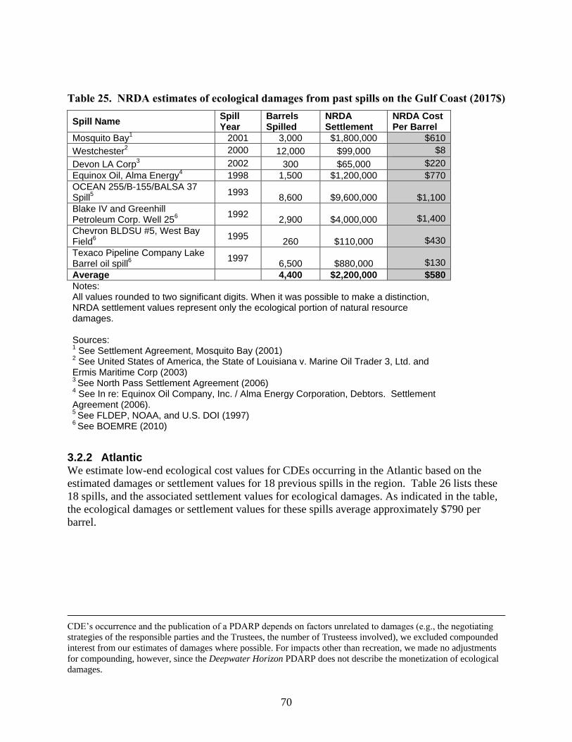
70

Table 25. NRDA estimates of ecological damages from past spills on the Gulf Coast (2017$)

Spill Name Spill Year

Barrels Spilled

NRDA Settlement

NRDA Cost Per Barrel

Mosquito Bay1

2001 3,000 $1,800,000 $610

Westchester2 2000 12,000 $99,000 $8

Devon LA Corp3 2002 300 $65,000 $220

Equinox Oil, Alma Energy4

1998 1,500 $1,200,000 $770

OCEAN 255/B-155/BALSA 37 Spill

5

1993 8,600 $9,600,000 $1,100

Blake IV and Greenhill Petroleum Corp. Well 25

6 1992 2,900 $4,000,000 $1,400

Chevron BLDSU #5, West Bay Field

6 1995 260 $110,000 $430

Texaco Pipeline Company Lake Barrel oil spill

6 1997 6,500 $880,000 $130

Average 4,400 $2,200,000 $580

Notes: All values rounded to two significant digits. When it was possible to make a distinction, NRDA settlement values represent only the ecological portion of natural resource damages. Sources: 1 See Settlement Agreement, Mosquito Bay (2001)

2 See United States of America, the State of Louisiana v. Marine Oil Trader 3, Ltd. and

Ermis Maritime Corp (2003) 3 See North Pass Settlement Agreement (2006)

4 See In re: Equinox Oil Company, Inc. / Alma Energy Corporation, Debtors. Settlement

Agreement (2006). 5 See FLDEP, NOAA, and U.S. DOI (1997)

6 See BOEMRE (2010)

3.2.2 Atlantic We estimate low-end ecological cost values for CDEs occurring in the Atlantic based on the

estimated damages or settlement values for 18 previous spills in the region. Table 26 lists these

18 spills, and the associated settlement values for ecological damages. As indicated in the table,

the ecological damages or settlement values for these spills average approximately $790 per

barrel.

CDE’s occurrence and the publication of a PDARP depends on factors unrelated to damages (e.g., the negotiating

strategies of the responsible parties and the Trustees, the number of Trusteess involved), we excluded compounded

interest from our estimates of damages where possible. For impacts other than recreation, we made no adjustments

for compounding, however, since the Deepwater Horizon PDARP does not describe the monetization of ecological

damages.

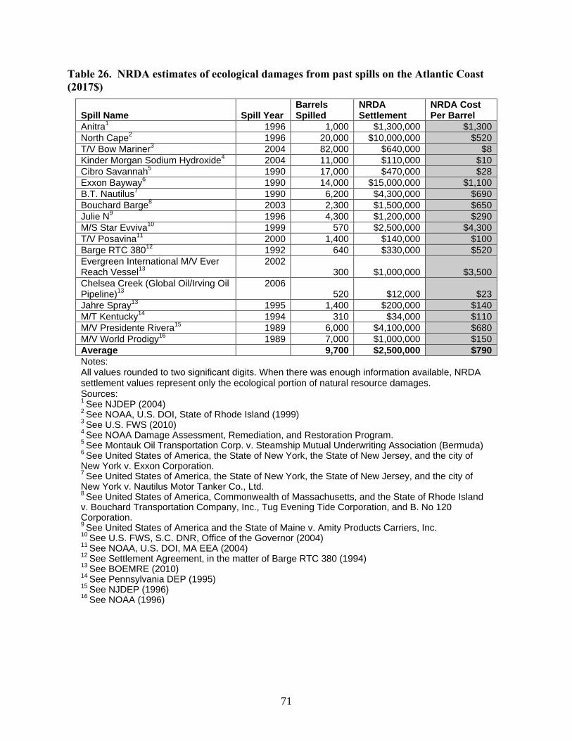
71

Table 26. NRDA estimates of ecological damages from past spills on the Atlantic Coast

(2017$)

Spill Name Spill Year Barrels Spilled

NRDA Settlement

NRDA Cost Per Barrel

Anitra1

1996 1,000 $1,300,000 $1,300

North Cape2

1996 20,000 $10,000,000 $520

T/V Bow Mariner3

2004 82,000 $640,000 $8

Kinder Morgan Sodium Hydroxide4

2004 11,000 $110,000 $10

Cibro Savannah5

1990 17,000 $470,000 $28

Exxon Bayway6

1990 14,000 $15,000,000 $1,100

B.T. Nautilus7

1990 6,200 $4,300,000 $690

Bouchard Barge8

2003 2,300 $1,500,000 $650

Julie N9

1996 4,300 $1,200,000 $290

M/S Star Evviva10

1999 570 $2,500,000 $4,300

T/V Posavina11

2000 1,400 $140,000 $100

Barge RTC 38012

1992 640 $330,000 $520

Evergreen International M/V Ever Reach Vessel

13 2002

300 $1,000,000 $3,500

Chelsea Creek (Global Oil/Irving Oil Pipeline)

13 2006

520 $12,000 $23

Jahre Spray13

1995 1,400 $200,000 $140

M/T Kentucky14

1994 310 $34,000 $110

M/V Presidente Rivera15

1989 6,000 $4,100,000 $680

M/V World Prodigy16

1989 7,000 $1,000,000 $150

Average 9,700 $2,500,000 $790

Notes: All values rounded to two significant digits. When there was enough information available, NRDA settlement values represent only the ecological portion of natural resource damages. Sources: 1 See NJDEP (2004)

2 See NOAA, U.S. DOI, State of Rhode Island (1999)

3 See U.S. FWS (2010)

4 See NOAA Damage Assessment, Remediation, and Restoration Program.

5 See Montauk Oil Transportation Corp. v. Steamship Mutual Underwriting Association (Bermuda)

6 See United States of America, the State of New York, the State of New Jersey, and the city of

New York v. Exxon Corporation.

7 See United States of America, the State of New York, the State of New Jersey, and the city of

New York v. Nautilus Motor Tanker Co., Ltd.

8 See United States of America, Commonwealth of Massachusetts, and the State of Rhode Island

v. Bouchard Transportation Company, Inc., Tug Evening Tide Corporation, and B. No 120 Corporation.

9 See United States of America and the State of Maine v. Amity Products Carriers, Inc.

10 See U.S. FWS, S.C. DNR, Office of the Governor (2004)

11 See NOAA, U.S. DOI, MA EEA (2004)

12 See Settlement Agreement, in the matter of Barge RTC 380 (1994)

13 See BOEMRE (2010)

14 See Pennsylvania DEP (1995)

15 See NJDEP (1996)

16 See NOAA (1996)

72

Ideally, the high-end estimate of ecological damages for a catastrophic spill in the Atlantic would

be estimated based on one or more historic examples of such a spill in the region. Since a

catastrophic oil spill has never occurred off the Atlantic coast of the United States, we estimate

the high-end costs of a catastrophic spill in the region by scaling the per barrel damages

associated with the Deepwater Horizon oil spill in the Gulf of Mexico. The sample of non-

catastrophic oil spills used to estimate low-end costs (presented in Tables 25 and 26) indicated

that the average oil spill in the Atlantic resulted in ecological damages per barrel 35 percent

higher than the average ecological damages in the Gulf of Mexico ($790 per barrel versus $580

per barrel). As a result, this analysis assumes that a catastrophic spill in the Atlantic would result

in ecological damages per barrel that are 35 percent greater than the damages from the

Deepwater Horizon spill. Scaling the Deepwater Horizon settlement value in this way suggests

that a catastrophic spill in the Atlantic would result in ecological damages of approximately

$3,000 per barrel

3.2.3 Cook Inlet While no catastrophic oil spills have occurred in Cook Inlet, the Exxon Valdez spill occurred in

the neighboring Prince William Sound. Because of the similarities between the two locations,18

we use the per barrel ecological damages associated with the Exxon Valdez spill as the high-end

estimate for the ecological damages expected to result from a catastrophic oil spill in Cook Inlet.

The Exxon Valdez settlement included approximately $1.1 billion to compensate for damages to

ecological resources, or approximately $4,200 per barrel of oil spilled (in year 2017 dollars).

A review of NRDAs led by NOAA and FWS did not identify any non-catastrophic spills in Cook

Inlet that might inform the estimation of a low-end ecological damages value for the area. In the

absence of such data, we develop a low-end estimate by scaling the low-end value for the Gulf of

Mexico by the ratio of ecological damages from Exxon Valdez compared to Deepwater Horizon.

Specifically, as noted above, the eight historic NRDAs in the Gulf of Mexico indicated average

ecological damages of $580 per barrel. Additionally, the Deepwater Horizon agreement indicates

ecological damages of $2,200 per barrel, while the Exxon Valdez settlement resulted in

ecological damages that were 86 percent higher, at $4,200 per barrel. As a result, we assume that

the low-end ecological damages for Cook Inlet are 86 percent greater than the average settlement

of $580 per barrel seen in the Gulf of Mexico, or $1,080 per barrel.

3.2.4 Arctic The uncertainty surrounding ecological damages is particularly high in the Arctic, given that

there is no historic record of NRDAs associated with oils spills of any size in the region. Since

the Arctic environment is most similar to that of Cook Inlet, the ecological damage estimates

produced for Cook Inlet serve as the starting point for the estimation of Arctic-specific values.

Lacking any historic spills to compare between the two regions, the OECM was used to develop

scaling factors to apply to the low-end and high-end values for Cook Inlet.

18 The similarities between the two locations were confirmed by outputs from the OECM. The BOEM

2017-2022 DPP scenario for Cook Inlet was run for both Cook Inlet and the Gulf of Alaska planning area, where

Prince William Sound is located. The OECM produced very similar estimates of ecological damages in both

planning areas (differing by only 2 percent), suggesting that oil spills tend to have similar impacts on the ecological

resources in each planning area.

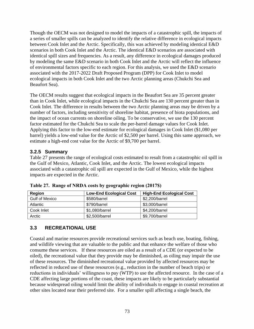
73

Though the OECM was not designed to model the impacts of a catastrophic spill, the impacts of

a series of smaller spills can be analyzed to identify the relative difference in ecological impacts

between Cook Inlet and the Arctic. Specifically, this was achieved by modeling identical E&D

scenarios in both Cook Inlet and the Arctic. The identical E&D scenarios are associated with

identical spill sizes and frequencies. As a result, any difference in ecological damages produced

by modeling the same E&D scenario in both Cook Inlet and the Arctic will reflect the influence

of environmental factors specific to each region. For this analysis, we used the E&D scenario

associated with the 2017-2022 Draft Proposed Program (DPP) for Cook Inlet to model

ecological impacts in both Cook Inlet and the two Arctic planning areas (Chukchi Sea and

Beaufort Sea).

The OECM results suggest that ecological impacts in the Beaufort Sea are 35 percent greater

than in Cook Inlet, while ecological impacts in the Chukchi Sea are 130 percent greater than in

Cook Inlet. The difference in results between the two Arctic planning areas may be driven by a

number of factors, including sensitivity of shoreline habitat, presence of biota populations, and

the impact of ocean currents on shoreline oiling. To be conservative, we use the 130 percent

factor estimated for the Chukchi Sea to scale the per-barrel damage values for Cook Inlet.

Applying this factor to the low-end estimate for ecological damages in Cook Inlet ($1,080 per

barrel) yields a low-end value for the Arctic of $2,500 per barrel. Using this same approach, we

estimate a high-end cost value for the Arctic of $9,700 per barrel.

3.2.5 Summary Table 27 presents the range of ecological costs estimated to result from a catastrophic oil spill in

the Gulf of Mexico, Atlantic, Cook Inlet, and the Arctic. The lowest ecological impacts

associated with a catastrophic oil spill are expected in the Gulf of Mexico, while the highest

impacts are expected in the Arctic.

Table 27. Range of NRDA costs by geographic region (2017$)

Region Low-End Ecological Cost High-End Ecological Cost

Gulf of Mexico $580/barrel $2,200/barrel

Atlantic $790/barrel $3,000/barrel

Cook Inlet $1,080/barrel $4,200/barrel

Arctic $2,500/barrel $9,700/barrel

3.3 RECREATIONAL USE

Coastal and marine resources provide recreational services such as beach use, boating, fishing,

and wildlife viewing that are valuable to the public and that enhance the welfare of those who

consume these services. If these resources are oiled as a result of a CDE (or expected to be

oiled), the recreational value that they provide may be diminished, as oiling may impair the use

of these resources. The diminished recreational value provided by affected resources may be

reflected in reduced use of these resources (e.g., reduction in the number of beach trips) or

reductions in individuals’ willingness to pay (WTP) to use the affected resource. In the case of a

CDE affecting large portions of the coast, these impacts are likely to be particularly substantial

because widespread oiling would limit the ability of individuals to engage in coastal recreation at

other sites located near their preferred site. For a smaller spill affecting a single beach, the

74

availability of substitutes in the same area may partially mitigate the recreational impact of the

spill. Given the potential scale and duration, a CDE could limit these substitution options.

Estimating the recreational value lost as a result of CDE requires information on (1) the baseline

level of activity for the full suite of recreational activities affected, (2) the change in the level of

recreational activity, and (3) the per unit (e.g., per user day or per beach trip) value that

individuals place on these activities in the baseline and during the impact period. This

information would allow one to estimate recreational value in the absence of the CDE and with

the CDE. Obtaining this information, however, presents a number of challenges, as described

below for each of the items outlined above.

Specification of baseline recreational resource use: The specification of the baseline would

ideally reflect use in the impacted area in the absence of a CDE. However, the timing

and location of a CDE, both of which are substantial determinants of a CDE’s impact, are

highly uncertain. With offshore oil production occurring year-round, a CDE could occur

during periods of high use or during periods when use is relatively low. Similarly, a CDE

could affect coastal and marine areas frequented by recreators or areas where recreation

is more limited.

Aside from uncertainties related to CDE location and timing, gauging baseline use is also

complicated by the fact that variables besides the occurrence of a CDE affect the use of

recreational resources. In particular, changes in weather affect the use of coastal

recreation sites, with higher temperatures and a lack of precipitation typically leading to

higher use than cooler temperatures and/or rain. Thus, even if use data are available for

an impacted area in the aftermath of a CDE, the prior year’s data may not be

representative of the actual baseline for that CDE. For example, if a hurricane had struck

during the prior year but not during the spill year, use during the prior year would likely

be an under-representation of baseline use.

Estimating the change in coastal recreation activity: Estimating changes in the use of

coastal resources attributable to a CDE is complicated by the non-spill factors described

in the baseline discussion above. Changes in the use of coastal recreation sites could

reflect the impact of a CDE as well as the weather, macroeconomic conditions, gas

prices, and other variables. Distinguishing between the influence of a CDE and these

other variables may not be possible in all cases. In addition, the spatial resolution of the

available use data may not allow one to focus exclusively on use in areas affected by a

CDE. For example, some data sources report use by state rather than for individual sites.

Valuation: The value of the recreational uses of coastal and marine resources is highly

variable depending on the attributes of the sites potentially affected by a CDE. Key

attributes that affect value include the amenities available at the site (e.g., fish pier), how

crowded a site is, the cleanliness of the site, or the prevalence of fish at the site (for

recreational fishing sites). Furthermore, because a CDE may affect the attributes of a

site, the value that individuals place on the site may change as a result of a CDE. Thus,

even if existing literature provides estimates of recreational value under non-CDE

conditions, the occurrence of a CDE could affect the value of recreational activity that

still takes place after the CDE occurs.

75

In addition to the challenges outlined above related to the measurement of baseline use, changes

in use associated with a CDE, and recreation value, the available data on each of these variables

is also fairly limited for most coastal areas. While use data are available from a few sources,

many of these sources are either outdated or limited in the scope of activities or geographic areas

that they cover. For example, the National Survey on Recreation and the Environment

(Leeworthy and Wiley, 2001), includes estimates of the number of user days for beach use, but

these data are for the year 2000 and are not disaggregated beyond the state level. Data on the

changes in use associated with a CDE are even more limited, as only two catastrophic spills have

ever occurred in the U.S. (e.g., the Exxon Valdez spill in 1989 and the Deepwater Horizon spill

in 2010). While data associated with these spills may inform the assessment of the recreational

impacts associated with a CDE, these events represent just two data points in a wide distribution

of recreational impacts that may occur as a result of a CDE. Finally, while the environmental

economics literature includes several studies related to the value of different coastal recreational

activities, many of these studies are fairly dated or focus on marginal changes on the value of

recreation that are not transferrable to assessment of the impacts of a CDE. For example, some

studies estimate changes in the value of a recreational fishing day per acre of coastal marsh

developed or preserved.

Despite these and other limitations, the available data nevertheless can be used to approximate

the potential recreational costs of a CDE for four recreational activities: beach use, recreational

fishing, boating (Gulf of Mexico only), and wildlife viewing (Cook Inlet only). We present our

estimates of these damages, on a per barrel basis, and our approach for developing these

estimates in the sections that follow. While a CDE would likely affect activities other than those

examined here, such as scuba diving, the available data for these other activities were insufficient

to support development of impact estimates.

3.3.1 Shoreline Recreation and Boating Our assessment of the potential per-barrel damages related to shoreline recreation (beach use and

inland fishing) and boating focuses on impacts in the Gulf of Mexico, the Atlantic, and Cook

Inlet.19

For the Gulf of Mexico region, we present the estimated damages associated with the

Deepwater Horizon spill as an indicator of potential impacts. We obtained this information from

the PDARP and the associated administrative record issued by the Deepwater Horizon Oil Spill

Natural Resource Trustees (the Trustees).20

The PDARP provides aggregate results from the

Trustees’ comprehensive study of the spill’s impacts on recreational activites, including

swimming, sunbathing, shoreline fishing, inland fishing, and boating. The Trustees’ assessment

of lost recreational use associated with the Deepwater Horizon spill represents one of the most

comprehensive and robust economic studies of coastal recreation ever conducted.

Due to the more limited data available for the Atlantic and Cook Inlet, we apply a different

approach for these regions. For both regions, we assume that a CDE would occur near the

beginning of the peak season for coastal recreation and would affect recreational activity for

several months. Based on this information, we develop estimates of baseline use in both areas

for an extended period of several months. We then estimate the percent reduction in use based

19 Aside from subsistence fishing, which we examine below, we are not aware of any recreational fishing

that takes place in the Arctic. 20 See NOAA (2015)

76

on the observed changes in use for the Deepwater Horizon and Exxon Valdez spills. Applying

these percentage reductions to the estimates of baseline use yields estimates of the lost user days

associated with a CDE. We value the reduction in recreational use based on estimates presented

in the economic literature. We present the details of this approach below by region.

Note that the recreational activity examined in this section includes beach use (inclusive of

fishing on sandy beaches), inland fishing, and boating. While much of the environmental

economics literature examines beach use and fishing separately, we examine them together here

because the most robust and detailed data that we identified combine the two.

Gulf of Mexico (GOM)

As noted above, we rely on the results of the lost recreational use assessment included in the

Deepwater Horizon (DWH) PDARP and the associated administrative record to approximate the

impacts of a CDE on coastal recreation in the Gulf of Mexio region. The DWH assessment

examines three categories of recreation: shoreline use, inland fishing, and boating. Shoreline use

includes any and all saltwater recreation occurring on sandy beaches, including swimming,

sunbathing, and fishing. Inland fishing, as distinct from shoreline fishing, represents fishing at

salwater locations not located on sandy beaches. Boating refers to pleasure boating and fishing

on motorboats or sailboats.

To estimate changes in recreational use associated with the spill, the Trustees mounted a

significant data collection effort that involved a series of onsite recreator surveys and aerial

counts of recreators partaking in recreationl activities at coastal sites. The Trustees measured the

number of recreators at 743 beach segments throughout the Gulf through overflights (conducted

by low-flying airplanes), and onsite interviews and counts (conducted by survey teams on foot).

To capture the impacts to recreational anglers at non-beach saltwater access points, the Trustees

sampled 323 sites from a list of non- beach saltwater sites provided by NOAA’s Marine

Recreational Information Program (MRIP). For the boating study, the Trustees conducted counts

and interviews to measure the number of recreational boaters entering the Gulf at 103 sites in the

North Gulf and 90 sites in the Florida Peninsula. Sites were selected from MRIP’s list of 534

saltwater boating access points open to the public. Using these various data, the study team

estimated the level of recreational activity during the impact period and after recreational use

returned to baseline levels. The difference between the two represents the change in use

associated with the spill.

The Trustees estimated the changes in shoreline recreation associated with the Deepwater

Horizon spill over a large area spanning the North Gulf and the Florida Pensinsula over a period

of 19 months. Figure 14 below shows a map of the sites sampled throughout the impact area

(including non-beach fishing and boating sites). The duration of spill impacts to recreation varied

within the area shown in Figure 14 and by activity. For example, the impact period for shoreline

use in the Florida Peninsula was June 2010 through January 2011, while the impact period for

shoreline use in the North Gulf (i.e., closer to the blowout site) was May 2010 through

November 2011. In addition, within the North Gulf, impacts for shoreline use were longer in

duration than impacts for inland fishing. Table 28 outlines the different impact periods by

activity and region.

77

Figure 14. Map of recreation sites sampled in the Deepwater Horizon lost recreational use

assessment21

Table 28. Duration of losses to shoreline recreation, by region and activity, for the

Deepwater Horizon lost recreational use assessment

2010 2011

Activity Region Ma

y

Ju

ne

Ju

ly

Au

g.

Se

pt.

Oct.

No

v.

De

c.

Ja

n.

Fe

b.

Ma

r.

Ap

r.

Ma

y

Ju

ne

Ju

ly

Au

g.

Se

pt.

Oct.

No

v.

Shoreline Use

North Gulf

Peninsula Inland

Fishing North Gulf

Boating North Gulf

Source: Adapted from NOAA (2015)

Tables 29 and 30 below, taken from the PDARP, present the recreational use estimates from

what the Trustees refer to as Tier 1 of the damage assessment.22

These Tier 1 damages are based

on the Trustee’s detailed infield data collection effort and cover the period June 2010 through

21 See NOAA (2015). 22 The Trustees’ Tier 2 estimates of damages, which rely on less detailed information than the Tier 1

estimates, as summarized below.

Source: NOAA (2015)

78

November 2011. Consistent with the PDARP’s presentation of results, Table 29 presents use

estimates for shoreline use and inland fishing combined. As shown in the table, the Trustees’

Tier 1 assessment estimated that the Deepwater Horizon spill resulted in 12.47 million lost user

days for shoreline use and inland fishing. This value represents a 23.3 percent reduction relative

to the baseline of 53.4 million user days over the entire 18-month impact period for Tier 1. Note

that Table 29 splits the impact period for shoreline use and inland fishing into two separate sub-

periods. For the first period—June 2010 through January 2011—the estimated reduction in use

is 32.5 percent, whereas the estimate for the second period—February 2011 through November

2011—is lower at 10.0 percent.

Table 29. Deepwater Horizon shoreline and inland fishing study lost use estimates – tier 1

Region Baseline Estimate

Spill Estimate (User Days During Spill)

Loss Estimate (Lost User Days)

Percent Decline

June 2010 through January 2011

North Gulf 14,207,507 7,782,270 6,425,237 45.2%

Peninsula 17,471,871 13,601,695 3,870,176 22.2%

Overall 31,679,378 21,383,965 10,295,413 32.5%

February 2011 through November 2011

North Gulf 21,754,732 19,580,582 2,174,149 10.0%

Total (Months 1-18) 53,434,109 40,964,547 12,469,562 23.3%

Source: NOAA (2015)

Table 30. Deepwater Horizon boating study lost use estimates - tier 1

Region Baseline

Boating Days

Boating Days During Spil

Impactperiod

Lost Boating

Days Percent Decline

North Gulf 759,605 544,231 215,374 28.4%

Source: NOAA (2015)

To estimate the economic value of recreational losses associated with the Deepwater Horizon

spill, the Trustees developed two Randomized Utility Maximization (RUM) models for saltwater

recreation in the Gulf of Mexico region. One model covers both shoreline use and inland

fishing, while the other is specific to boating. These models capture the value of lost trips, as

well as the value of substitute trips and diminished-value trips (i.e., trips that still occurred with

the spill but were of lesser value because of the spill). The Trustees collected the data necessary

to estimate these models from a local survey targeting adults who live in Louisiaina, Mississippi,

Alabama, Florida, and selected counteies in Texas and Georgia, and a national survey that

targeted adults living in the contiguous U.S., excluding the areas targeted in the local survey.

79

Using the survey data, the valuation models provide a quantitative description of people’s

recreation behavior. For example, the shoreline valuation model estimates the number of

recreation trips from throughout the contiguous U.S. to different shoreline areas in the Gulf of

Mexico region. This behavior, combined with the costs associated with different site choice

options, form the basis of the models’ valuation of recreation. Calibrating the models to the

reduction in use measured through the overflights and infield surveys (see Tables 29 and 30), the

Trustees estimated a value per lost user day of $36.25 for shoreline use and inland fishing and

$16.20 per day for boating, both in year 2015 dollars.23

In year 2017 dollars, these values are

$37.87 and $16.93, respectively. When applied to the lost user day estimates presented above in

Tables 29 and 30, this translates to losses of more than $475 million in total, as summarized in

Table 31.

Table 31. Summary of Tier 1 recreation impacts associated with the Deepwater Horizon

spill

Lost User Days

Value Of Recreation Impacts (2017$)

Shoreline 12,325,512 $466,800,000

North Gulf 8,455,336 $320,200,000

Peninsula 3,870,176 $146,600,000

Inland Fishing 144,050 $5,500,000

Boating 215,374 $3,600,000

Total $475,900,000

Note: The value of recreation impacts presented in this table is lower than the

estimate of approximately $523 million in the PDARP for the Deepwater Horizon

spill. The difference reflects the compounding of damages from 2010 to 2015 in

the PDARP. For the purposes of the present analysis, we do not compound

impacts.

Source: Values derived from English and McConnell (2015). Values from this

memorandum were converted to year 2017 dollars.

The Tier 1 losses shown in Table 31 reflect the extensive infield data collection undertaken by

the Trustees. The coverage of the infield studies, however, does not include all locations, times

of day, or months impacted by the spill. For example, the study team’s primary infield data

collection did not capture use of the beach at night. To address these gaps in coverage, the

Trustees performed a series of supplemental analyses using various other data sources. These

Tier 2 analyses and the losses estimated by each analysis are summarized in Table 32.

23 Please see Appendix B for a summary of additional GOM beach use and fishing valuation estimates.

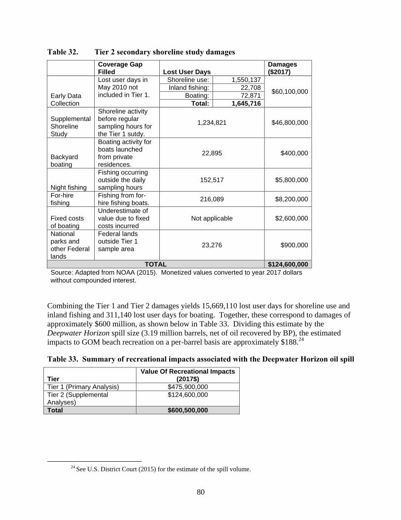
80

Table 32. Tier 2 secondary shoreline study damages

Coverage Gap Filled Lost User Days

Damages ($2017)

Early Data Collection

Lost user days in May 2010 not included in Tier 1.

Shoreline use: 1,550,137

$60,100,000 Inland fishing: 22,708

Boating: 72,871

Total: 1,645,716

Supplemental Shoreline Study

Shoreline activity before regular sampling hours for the Tier 1 sutdy.

1,234,821 $46,800,000

Backyard boating

Boating activity for boats launched from private residences.

22,895 $400,000

Night fishing

Fishing occurring outside the daily sampling hours

152,517 $5,800,000

For-hire fishing

Fishing from for-hire fishing boats.

216,089 $8,200,000

Fixed costs of boating

Underestimate of value due to fixed costs incurred

Not applicable $2,600,000

National parks and other Federal lands

Federal lands outside Tier 1 sample area

23,276 $900,000

TOTAL $124,600,000

Source: Adapted from NOAA (2015). Monetized values converted to year 2017 dollars

without compounded interest.

Combining the Tier 1 and Tier 2 damages yields 15,669,110 lost user days for shoreline use and

inland fishing and 311,140 lost user days for boating. Together, these correspond to damages of

approximately $600 million, as shown below in Table 33. Dividing this estimate by the

Deepwater Horizon spill size (3.19 million barrels, net of oil recovered by BP), the estimated

impacts to GOM beach recreation on a per-barrel basis are approximately $188.24

Table 33. Summary of recreational impacts associated with the Deepwater Horizon oil spill

Tier Value Of Recreational Impacts

(2017$)

Tier 1 (Primary Analysis) $475,900,000

Tier 2 (Supplemental Analyses)

$124,600,000

Total $600,500,000

24 See U.S. District Court (2015) for the estimate of the spill volume.

81

Atlantic

As noted above, the impacts of a CDE on coastal recreation will depend on when and where a

CDE occurs. For the purposes of estimating the recreational impacts of a CDE in the Atlantic

OCS Region, we assume that a CDE would affect recreation in the states along the Mid-Atlantic

OCS Planning Area. Based on BOEM’s 2017 – 2022 Draft Program Proposal, more than 80

percent of the undiscovered technically recoverable resources (UTTR) of the Program Area are

in the Mid-Atlantic.25

Thus, the Mid-Atlantic represents the portion of the Atlantic region most

at risk to a CDE. As a sensitivity analysis, however, Appendix A examines the recreational

impacts of a scenario in which a CDE in the Atlantic affects coastal recreation in the Mid-

Atlantic and as far north as New Jersey. The sensitivity analysis also considers another scenario

in which a CDE in the Atlantic affects recreation in Georgia and South Carolina, as well as the

Mid-Atlantic.

In addition to a CDE’s location, its timing and the duration of its impact are also highly

uncertain. As a simplifying assumption, this analysis examines the impacts of a hypothetical

CDE in the Atlantic with timing and duration of impacts consistent with the Deepwater Horizon

spill in the Gulf of Mexico. Specifically, we assume that the CDE would occur in the spring and

would affect shoreline recreation (beach use and fishing on sandy beaches) and inland fishing as

follows:

Shoreline recreation: We assume that the CDE would affect shoreline recreation from

May of the year that the spill occurs through November of the following year. This time

horizon is consistent with the duration of shoreline impacts in the North Gulf following

the Deepwater Horizon spill (see Table 28 above). While it is possible that the duration

of impacts may be shorter for areas relatively far from the CDE site (i.e., similar to the

Florida peninsula for the Deepwater Horizon spill), we assume a 19-month impact period

consistent with that for the North Gulf to avoid potential underestimation of impacts.

In specifying shoreline recreation in the baseline, we split the 19-month period into two

sub-periods: May to January and February to November. As described in greater detail

below, we assume different percent changes in use for these two periods, based on the

changes observed following the Deepwater Horizon spill.

Inland fishing: We assume that a CDE in the Mid-Atlantic and would affect inland

fishing from May of the spill year through March of the following year across the entire

area. This time horizon is consistent with the assessment of inland fishing impacts for the

Deepwater Horizon spill.

Note that our quantitative assessment of potential recreational impacts in the Atlantic does not

include boating impacts. While a CDE is likely to affect boating in the Atlantic, the available

data on boating in this region are limited. In addition, the results of the Deepwater Horizon lost

recreational use assessment suggest that boating impacts are small relative to impacts related to

beach use and fishing.

25 See BOEM (2015).

82

To develop an estimate of baseline beach use for the Mid-Atlantic region, we rely on beach

recreation data from the 2000 National Survey of Recreation in the Environment (NSRE).26

The

NSRE is a comprehensive survey of outdoor recreation participation in the United States and was

conducted by the U.S. Forest Service and NOAA. The results of the survey include estimates of

beach visitor days by state for the year 2000. To estimate the percentage of annual beach visits

occurring during the May – January period, we examined the National Park Service’s monthly

visitation data for 2009–2014 for Assateague Island National Seashore (Maryland), Cape

Hatteras National Seashore (North Carolina), and Cape Lookout National Seashore (North

Carolina).27

Based on these monthly data, we estimate that 88 percent of annual visitation at

National Seashores in the Mid-Atlantic occurs between May and January. Under the assumption

that this value applies to all beaches in Delaware, Maryland, North Carolina, and Virginia, we

estimate baseline beach visitation during the May through January period of 68.6 million beach

days. Using visitation data for the same National Seashores, we estimate that 96 percent of

annual visitation on the Atlantic occurs between February and November. Applying this value to

the NSRE data, we estimate 74.9 million beach trips to the states included in our study for the

February-November period. Taken together, we estimate a total baseline beach visitation of

143.5 million beach days across the two sub-periods. (i.e., May to January and February to

November). Table 34 presents our baseline estimates for the Mid-Atlantic. To provide

additional perspective on use in the Mid-Atlantic, the table also includes baseline estiamtes for

New Jersey, South Carolina, and Georgia.28

The latter two are near the Program Area, but the

waters offshore from these states contain less than 20 percent of the UTTR in the Program Area,

as noted above.

Table 34. Beach use baseline for the Atlantic

State

Estimated Number of Beach Visits

May – January

Estimated Number of Beach Visits

February – November

Total Beach Visits May of Spill Year – November of The Following Year

Delaware 11,290,000 12,320,000 23,620,000

Maryland 16,400,000 17,890,000 34,290,000

Virginia 16,440,000 17,940,000 34,380,000

North Carolina 24,500,000 26,730,000 51,230,000

Mid Atlantic Total 68,630,000 74,880,000 143,520,000

BEACH USE IN OTHER STATES IN THE ATLANTIC

New Jersey (North Atlantic)

35,850,000 39,120,000 74,970,000

South Carolina (South Atlantic)

29,210,000 31,870,000 61,070,000

Georgia (South Atlantic)

7,440,000 8,120,000 15,560,000

We estimate baseline use for inland fishing for the Atlantic Program Area based on inland angler

trip data from NOAA’s MRIP.29

NOAA’s MRIP was initiated in 2007 and generates estimates of

26 See Leeworthy and Wiley (2001). 27 See NPS (2014). 28 Baseline data are only presented for periods in which impacts are expected. 29 See NOAA (2014). Note that we use only the inland angler data from MRIP rather than total angling.

We do not use the data for all angling to avoid potential double counting of anglers that are likely to be reflected in

83

angler’s catch and effort; the data are collected in six two-month periods (i.e. waves). Angler trip

data for Wave 1 (January and February), Wave 2 (March and April), Wave 3 (May and June),

Wave 4 (July and August), Wave 5 (September and October), and Wave 6 (November and

December) were downloaded for the Mid – Atlantic states, as well as for New Jersey, South

Carolina, and Georgia for the years 2009 – 2014. To limit the angler trip data to the assumed

impact period of a CDE (May – March), we divide Wave 2 data data for each year and state by

two, assuming that fishing activity is evenly split between the two months in each wave. For

every state and wave, we then calculate the average number of angler trips across the six years

for which we compiled data. For example, we average the number of angler trips taken during

Wave 3 (May and June) in Delaware across the years 2009, 2010, 2011, 2012, 2013, and 2014.

We then sum the wave-level averages for each state to determine the average number of trips

during the assumed impact period (May – March). Summing across states, we estimate slightly

less than 7.13 million baseline angler trips for the Mid-Atlantic region, as shown in Table 35

below.

Table 35. Recreational inland angler trips baseline for the Atlantic : May – March impact

period30

State Estimated Number of Angler Trips

May – March

Delaware 650,000

Maryland 2,410,000

Virginia 2,230,000

North Carolina 1,830,000

Mid Atlantic Total 7,130,000

INLAND FISHING IN OTHER STATES IN THE ATLANTIC

New Jersey (North Atlantic) 2,570,000

South Carolina (South Atlantic) 980,000

Georgia (South Atlantic) 620,000

To estimate the change in recreation associated with a CDE in the Atlantic Program Area, we

assume that proportional changes in recreational activity estimated in the Gulf of Mexico due to

the Deepwater Horizon spill would also apply to the Atlantic. Thus, consistent with the data

presented above in Table 29 for shoreline use and inland fishing, we assume that a CDE

occurring in the spring would lead to a 32.5 percent reduction in shoreline use and inland fishing

combined from May through January across the entire mid-Atlantic.31

For February through

November during the year following the CDE, we assume a 10 percent reduction in use. Based

on these assumptions and the baseline data presented above in Tables 34 and 35, we estimate that

the NSRE data that we use to estimate beach visitation. Because the beach visitation data in the NSRE includes any

activities on the beach, the NSRE documentation (Leeworty and Wiley 2001) cautions against adding beach

visitation data to other activities. Because inland fishing by definition does not occur on sandy beaches, anglers

involved in inland fishing are unlikely to be reflected in the NSRE data for beach recreation. 30 Please see Appendix A for additional damage estimates associated with a spill that affects NJ, SC, and

GA. 31 Ideally, we would derive separate estimates of the percent reduction in use for shoreline use and inland

fishing. The PDARP and associated administrative record for the Deepwater Horizon spill, however, do not include

baseline estimates for inland fishing alone. Instead, the baseline data include shoreline use and inland fishing

together.

84

a CDE in the Atlantic would result in a total of 29.8 million lost beach days and 2.2 million lost

inland fishing trips, as summarized in Table 36.

Table 36. Estimated reduction in recreational activitity in the Atlantic following a CDE

State Estimated Reduction in

Shoreline Visits Estimated Reduction in

Inland Fishing Trips

Delaware 4,900,000 210,000

Maryland 7,120,000 750,000

Virginia 7,140,000 700,000

North Carolina 10,640,000 570,000

TOTAL 29,790,000 2,230,000

We estimate the value of lost recreational use in the Atlantic based on the results of studies from

the empirical environmental economics literature. For beach use, we rely on three specific

studies from this literature. Parsons (2003) estimates $25 per lost trip (in 2003 dollars)

associated with closing all Delaware beaches to Delaware residents. Based on the results of

another study by Parsons (2000), the damage assessment of lost human use for the Buzzards Bay

oil spill applies a per beach trip value of $28.02 in 1997 dollars.32

Focusing on the value of

seven different beaches in North Carolina, Bin (2004) estimates user day values ranging from

$21 to $72 for these beaches.33

Averaging across these studies and converting to year 2017

dollars, we estimate a value of $47.21 per activity day. Applying this value to the estimated

reduction in beach visitor days associated with a CDE, we estimate a loss in the value of beach

recreation of $1.4 billion for the Mid-Atlantic region, as shown in Table 37.

To estimate the value of the reduction in inland fishing in the Atlantic, we apply value-per-trip

estimates obtained from two valuation studies that focus specifically on this region. McConnell

and Strand (1994) estimate a mean WTP for one day fishing trips by wave (e.g., March/April,

May/June, etc.) for nine east coast states, with an average of $81.82 across all states and waves

(in 1988 dollars). Whitehead and Haab (2000) estimate a median compensating variation per trip

for site access in North Carolina of $1.08 in 2000 dollars.34

Averaging across studies and

converting to year 2017 dollars yields an estimated value of $78.00 per fishing trip.35

Based on

this value and the 2.2 million lost fishing trips estimated above, we estimate approximately $174

million in inland fishing losses for the Mid-Atlantic region.

Table 37. Summary of recreational damages associated with a CDE in the Atlantic

Damage Category Estimated Damages

(2017$)

Shoreline Use $1,407,000,000

Inland Fishing $174,000,000

TOTAL $1,580,000,000

32 This value was derived using a model that was originally developed by Parsons (2000), The model was

adapted for use in the Buzzards Bay assessment. 33 See Parsons (2003), Bin (2004) and Bouchard B-120 Oil Spill Lost Use Technical Working Group

(2009) 34 See McConnell and Strand (1994) and Whitehead and Haab (2000). 35 Note, we keep the separate WTP values in McConnell and Strand separate when calculating the average.

85

To estimate recreational damages on a per-barrel basis, we divide the estimated shoreline and

inland fishing damages by by the spill volume associated with the Deepwater Horizon spill (3.19

million barrels) 36

, which results in an estimate of $441 per barrel for shoreline use and $54 per

barrel for inland fishing, both in year 2017 dollars. While the spill volume associated with a

CDE in the Atlantic may differ from the volume associated with the Deepwater Horizon

blowout, we determined that this would be the most appropriate spill volume to use given that

our analysis for the Atlantic uses the percentage reduction in shoreline use for the Gulf of

Mexico.

Cook Inlet

For Cook Inlet, our assessment of the shoreline recreational impacts of a CDE is limited to

recreational fishing, as beach use is likely to be minimal in the area’s relatively cool climate.

Similar to our approach for assessing recreational fishing impacts in the Gulf of Mexico and the

Atlantic, we estimate baseline use, approximate the proportional change in use, and apply

estimates from the empirical economics literature to value these changes. The data sources that

we apply for Cook Inlet, however, differ significantly from those applied in the Gulf of Mexico

and the Atlantic, as detailed below.

To estimate the baseline number of recreational fishing trips in Cook Inlet, we use data on the

annual number of saltwater angler days in Cook Inlet from the Alaska Department of Fish and

Game’s Sport Fishing Survey. 37

The Department’s Sport Fish Division has conducted the survey

annually by mail since 1977 and uses the data collected to estimate the state’s sport fishing

harvest by species and the total level of sport fishing activity. Using annual Cook Inlet data from

the Survey for 2009-2013, we arrive at an average baseline of 172,600 angler trips.

As an indicator of the potential reduction in recreational fishing in Cook Inlet in response to a

CDE, we assume that the reduction observed in southcentral Alaska following the Exxon Valdez

spill would also apply to recreational fishing in Cook Inlet. Based on the Alaska Department of

Fish and Game’s annual survey of Alaska anglers, Mills (1992) estimates that the Exxon Valdez

spill led to a 14.9 percent reduction in fishing trips between 1988 and1989 in the area affected by

the spill. Applying this percent reduction to the Cook Inlet baseline of 172,600 angler trips

results in a total of 25,800 angler trips lost due to a CDE.

To place a value on angler days in Cook Inlet, we draw from the values estimated in two studies:

Hamel (2000) and Hausman (1995). Hamel (2000) estimates the mean compensating variation

per fishing day for Central and Lower Cook Inlet for both Alaskans ($81.47 in year 1997 dollars)

and nonresidents ($119.79 in year 1997 dollars). Together, the average compensating variation in

year 2017 dollars is $155. In the context of the Exxon Valdez spill, Hausman (1995) estimates a

1989 consumer surplus per sport fishing trip of $148. Inflated to 2017 dollars, this estimate is

$296. Averaging across studies, we arrive at $226 per fishing trip in year 2017 dollars. Applying

this value to the estimated loss of 25,800 angler trips lost from a CDE results in total damages of

$5.8 million. On a per-barrel basis (using the spill size from Exxon Valdez of 257,000 barrels),

estimated loses are $22.62 in 2017 dollars. We use the spill volume from the Exxon Valdez spill

36 See U.S. District Court (2015). 37 See ADFG (2013).

86

to calculate damages on a per barrel basis because the percentage reduction in recreational

fishing reflected in our damages estimate is based on the impact of the Valdez spill.

3.3.2 Wildlife Viewing

In addition to impacting beach use and recreational fishing, a CDE may also affect recreational

wildlife viewing in coastal areas. Our assessment of the impacts of a CDE on wildlife viewing

focuses on Cook Inlet, as wildlife viewing represents an appreciable portion of coastal recreation

in the area. We were unable to identify wildlife viewing data specific to Cook Inlet, but such

data are available in aggregate for southcentral Alaska. Because Cook Inlet makes up a

substanstial portion of southcentral Alaska and offers an abundance of wildlife viewing

opportunities, we apply the data for southcentral Alaska as an indicator of wildlife viewing in

Cook Inlet.

To develop an estimate of baseline wildlife viewing, we integrate data from several sources,

based on the following three-step approach.

1. Estimate visitation to southcentral Alaska: As an initial step in estimating the baseline

level of wildlife viewing on an annual basis, we estimate the total visitation to

southcentral Alaska in the typical year. Based on visitation data for the years 2009

through 2014 from the McDowell Group (2014), we estimate that there are

approximately 1,605,000 non-resident trips to Alaska each year on average. An earlier

report published by the McDowell Group (2011) also states that 56 percent of visitors to

Alaska visit southcentral Alaska.38

Applying this value to the total number of visitors to

the state, we estimate that approximately 899,000 individuals visit southcentral Alaska

each year. While much of the wildlife viewing in southcentral Alaska may be in areas

other than Cook Inlet, we use these data to develop a conservative (i.e., potentially high

end) estimate of the potential impacts of a CDE in Cook Inlet.

2. Estimate number of visitors to southcentral Alaska engaged in wildlife viewing: The

McDowell Group (2011) also indicates that 52 percent of visitors to Alaska engage in

wildlife viewing. Based on this value and the estimated 899,000 visitors to southcentral

Alaska on an annual basis, we estimate that approximately 467,400 visitors to

southcentral Alaska engage in wildlife viewing on an annual basis.

3. Estimate wildlife viewing days: To translate the number of wildlife viewing visitors to

the number of wildlife viewing days in southcentral Alaska, we derive a multiplier using

valuation data from the U.S. Fish and Wildlife Service (2009). While the FWS study

focuses on valuation rather than visitation, the values estimated by FWS for nonresident

wildlife viewing in Alaska include the mean economic value per year per visitor and the

value per day per visitor. Assuming that each visitor takes one trip to Alaska per year,

dividing the former by the latter yields an estimate of the average number of wildlife

viewing days per trip. Following this approach, we estimate six days per wildlife

viewing trip. Applying this value to the number of visitors presented above (467,400), we

estimate an average of 2,764,000 wildlife viewing days in southcentral Alaska. We note

38 See McDowell Group (2011).

87

the possibility that the estimate of six days per trip could be an overestimate if the

economic value per year from FWS reflects activities other than wildlife viewing.

Nevertheless, in the interest of developing a conservative (i.e., potentially high end)

estimate, we applied the FWS data assuming that the data reflect wildlife viewing only.

Consistent with BOEM’s 2012 analysis of catastrophic spill impacts, we assume a high-impact

spill scenario in which a CDE occurs in the summer and last for 80 days, which represents 53

percent of the summer season.39

Based on this value and assuming that wildlife viewing is

uniformly distributed over the summer season, we estimate that 1.5 million wildlife viewing days

will be affected by a CDE in the Cook Inlet Area. To estimate the economic value of these

losses, we assume that half of the value of a wildlife viewing day will be lost for affected trips.

Applying this assumption to the FWS (2009) estimate of the mean per-day value of wildlife

viewing in Alaska for non-residents ($129 adjusted to year 2017 dollars), we estimate a loss of

approximately $65 per affected viewing day. Thus, we estimate wildlife viewing losses in Cook

Inlet of approximately $94.6 million.40

Because the assumptions specified in this section may

apply to CDEs of varying sizes, we do not express these damages on a per barrel basis.

3.4 COMMERCIAL FISHING

The occurrence of a CDE could have wide-ranging impacts on commercial fisheries in the

affected region. Most directly related to the supply of commercially harvested species, exposure

to discharged oil may result in several adverse effects to these species, such as premature

hatching, reduced growth rates, genetic abnormalities, and mortality, each of which would

contribute to reduced landings (Sumaila et al., 2012). In addition to these direct effects, indirect

exposure to discharged oil through the food web may adversely affect the condition and/or

abundance of harvested species. Even if vessel operators are able to maintain landings at

historical levels in the face of these direct and indirect effects, the cost of achieving these

landings may increase, putting upward pressure on seafood prices. With respect to demand,

consumers may reduce their consumption of seafood in response to a spill to avoid real or

perceived risks associated with consuming contaminated seafood. In effect, consumers’ WTP

for seafood (i.e., the value that they derive from seafood) may fall, at least temporarily, as a

result of a spill.

Accurately estimating the welfare losses associated with the commercial fishery impacts of a

CDE would require detailed information on affected fisheries, both before the spill and in its

aftermath. In particular, such an analysis would require information on changes in landings,

production costs, consumption, and pricing. Gauging the changes in these variables, however, is

fraught with uncertainty. Depending on the timing and location of a CDE, changes in landings

could vary. For example, a spill that occurs in close proximity to a fishery immediately before

the start of the fishing season would likely lead to higher impacts to landings than spills farther

away from fisheries at the end of the season. The extent to which vessel operators are able to

make operational changes to minimize the impact of a spill is also likely to vary. Fishermen

harvesting mobile species that limit their exposure to discharged oil might be able to fish in areas

not impacted by the spill and achieve the same or similar landings as they would absent the spill,

whereas such a change may not be possible in fisheries for oysters and other less mobile species.

39 See BOEM (2012). 40 See BOEM (2012).

88

Other examples of potential mitigating behaviors, the success of which would vary depending on

the circumstances, include switching to other species or fishing earlier or later in the season.

The reaction of seafood consumers to a CDE is also highly uncertain. While the literature

includes demand functions for several harvested species41

, the occurrence of a CDE could

fundamentally change these functions in uncertain ways for an unspecified period of time.

Factors affecting these changes may include the size of the area oiled, the species potentially

affected by oiling, and consumer attitudes regarding the potential risks of consuming

contaminated seafood. Because of the limited number of CDEs to have occurred historically, the

nature of the changes in demand due to these and other factors is unknown.

3.4.1 Commercial Fishing Approach

Due to the uncertain magnitude of the changes in seafood prices, production costs, and demand

functions that would result from a CDE, we present estimated changes in revenues—rather than

changes in producer and consumer surplus—as the metric of impacts for the commercial fishing

sector. For each region—the Gulf of Mexico, the Atlantic, and Cook Inlet—we compiled recent

landings data to serve as the baseline.42

We then estimated the reduction in landings for each

region based on a series of region-specific assumptions, as described in greater detail below.

Gulf of Mexico

To estimate the reduction in commercial fishery revenues associated with a CDE in the Gulf of

Mexico, we draw from the observed changes in commercial fisheries in response to the

Deepwater Horizon spill. Based on historical landings data published by NOAA’s National

Marine Fisheries Service (NMFS)43

, we estimate that the total volume of landings in 2010 in the

Gulf was approximately 22 percent lower than the average of the three previous years (2007

through 2009). Using a slightly different baseline of 2008-2009 and 2011-2013, the estimated

reduction in the volume of landings increases to 25 percent, as summarized in Table 38. When

measured in terms of revenues rather than volume, the landings impacts of the Deepwater

Horizon spill are lower than the estimated changes in volume. As shown in Table 39, we

estimate that landings revenues declined by 8 to 16 percent as a result of the spill, depending on

the years used as the baseline. This lower impact may reflect an increase in prices associated

with the spill-related reduction in harvests.

41 For example, see Blomo et al., 1982 and Houston et al., 1989 for demand of Gulf of Mexico shrimp and

Park et al., 2004 for demand of snapper/grouper. 42 Commercial fishing is currently banned in the Arctic. 43 See NOAA/NMFS (undated).

89

Table 38. Estimated change in Gulf of Mexico landings volume following the Deepwater

Horizon oil spill

Species

Change in Volume of Landings in 2010

Relative to 2007-2009

Change in Volume of Landings in 2010 Relative to

2008-2009 And 2011-2013

Mehhaden 102,100 metric tons

(-23%) 135,900 metric tons

(-28%)

Shrimp 19,300 metric tons

(-19%) 17,200 metric tons

(-17%)

Eastern Oysters 2,800 metric tons


(-23%)

Blue Crab 6,800 metric tons


(-22%)

Other 5,500 metric tons


(-14%)

TOTAL 136,500 metric tons

(-22%) 166,200 metric tons

(-25%)

Note: Values in first line of each cell represent the change in landings measured in metric tons. The value in parentheses represents the percent change in landings. Source: Data based on landings data reported by NOAA/NMFS.

Table 39. Estimated change in Gulf of Mexico landings revenue following the Deepwater

Horizon oil spill

Species

Change in Landings Revenue in 2010 Relative to 2007-

2009

Change in Landings Revenue in 2010 Relative to

2008-2009 and 2011-2013

Mehhaden $14,000,000

(-19%) $25,300,000

(-30%)

Shrimp $27,600,000

(-7%) $68,000,000

(-15%)

Eastern Oysters $16,600,000

(-21%) $14,900,000

(-19%)

Blue Crab $4,200,000

(-8%) $7,100,000

(-13%)

Other $2,500,000

(-2%) $16,200,000

(-9%)

TOTAL $64,900,000

(-8%) $131,600,000

(-16%)

Note: Values in first line of each cell represent the change in landings revenue measured in year 2017 dollars. The value in parentheses represents the percent change in landings revenue.

For the purposes of estimating the impacts associated with a future CDE, we assume a 16 percent

reduction in landings revenue, consistent with the higher of the two values shown in Table 39.

We use the estimated percentage change in landings revenue rather than the percent change in

landings volume because the change in landings revenue is our metric of impacts in the absence

of information that would allow us to estimate changes in producer and consumer surplus.

Applying the 16 percent value to the average of landings revenues for 2011 through 2013, the

90

thee most recent years for which data are available, we estimate commercial fishery damages of

$131 million (year 2017$). Based on the estimated 3.19 million barrels of oil spilled and not

recovered as a result of the Deepwater Horizon blowout, this value translates to $40.92 in

commercial fishing damages per barrel spilled.

Atlantic

To estimate the commercial fishing impacts of a CDE in the Atlantic, we rely on the impacts

estimated for the Gulf of Mexico following the Deepwater Horizon blowout and spill. More

specifically, we assume that the proportional change in landings revenues estimated for the Gulf

of Mexico in the aftermath of the Deepwater Horizon spill (16 percent) also applies to the

commercial fishing impacts of a CDE occurring in the Atlantic. We apply this proportional

change in landings revenues to fisheries in the states neighboring the Mid-Atlantic OCS planning

area, consistent with our approach for recreational impacts. If a CDE were to occur in the

Atlantic, it is unlikely that it would affect all fisheries in the Atlantic. As noted above, BOEM’s

2017 – 2022 Draft Program Proposal indicates that approximately 80 percent of the UTTR of the

Atlantic Program Area are in the Mid-Atlantic.44 Based on this information, we focused on

fisheries in the Mid-Atlantic.

Table 40 presents the landings revenues reported by NMFS for the four states that neighbor the

Mid-Atlantic Planning Area (North Carolina, Virginia, Maryland, and Delaware) and our

estimates of the change in landings associated with a CDE. As indicated in the table, baseline

landings are approximately $368.4 million per year. Note that many of the species shown in the

table are typically caught in embayments or other areas close to shore, far removed from

potential well sites on the OCS. However, because a catastrophic spill could occur from a tanker

transporting oil to shore, including these nearshore fisheries in the assessment is appropriate. As

indicated in the table, based on the available data, we estimate that a CDE would lead to a $57.6

million reduction in landings. Based on this value and the 3.19 million barrels of unrecovered oil

discharged during the Deepwater Horizon spill, we estimate that a CDE in the Atlantic would

lead to commercial fisheries damages of $18.06 per barrel.

As additional perspective on the baseline landings data shown in Table 40 for the Mid-Atlantic,

we note that NMFS estimates annual landings of approximately $237 million for New Jersey,

South Carolina, and Georgia combined—three states that could potentially be affected by a CDE

in the Atlatnic Program Area. Approximately 83 percent of these landings represent commercial

fishing activity in New Jersey.

44 See BOEM (2015).

91

Table 40. Commercial fishery landings revenue in the mid-Atlantic (2017$)

Species

Average Annual Landings Revenue: 2011-2013

1

Estimated Change in Landings Revenue Due to a Catastrophic Spill

Blue Crab $121,100,000 $18,900,000

Scallops $61,200,000 $9,600,000

Menhaden $33,700,000 $5,300,000

Eastern Oyster $26,000,000 $4,100,000

Striped Bass $15,000,000 $2,300,000

Flounder $17,000,000 $2,700,000

Other $94,500,000 $14,800,000

TOTAL $368,400,000 $57,600,000

Notes:

1. 2011-2013 landings revenue from the NMFS.

Cook Inlet

Our approach for estimating the commercial fishing impacts of a CDE in Cook Inlet reflects the

unique geographic features of Cook Inlet relative to the Gulf of Mexico and the Atlantic. More

specifically, because Cook Inlet is small relative to the Gulf of Mexico and Atlantic and has

limited access to open water, we assume that a catastrophic spill in Cook Inlet would affect all

fisheries in the area and that a full year’s landings would be lost. Table 41 presents the average

annual ex-vessel revenues over the 2012-2014 period (the three most recent years for which data

are available). Based on the data in the table, we estimate that a catastrophic spill in Cook Inlet

would result in $43.5 million in commercial fisheries damage. Because these impacts could be

realized across a wide range of spill volumes, we do not generate a per barrel estimate of

damages.

Table 41. Average annual Cook Inlet commercial fishery landings (2017$)

Species Average Annual Ex Vessel

Value: 2012-20141

Chinook $338,000

Sockeye $40,271,000

Coho $752,000

Pink $1,264,000

Chum $904,000

TOTAL $43,528,000

Source: ADFG (2014).

3.5 SUBSISTENCE

Many coastal communities throughout the United States rely on coastal and marine natural

resources for subsistence. In particular, Native Alaskan communities in Cook Inlet and the Arctic

depend on resources such as Bowhead whales and other marine species to meet their basic needs.

Oil released during a CDE may contaminate large portions of the Alaskan coastal and marine

environment, making it impossible for communities to subsist on the resources that are normally

available. These communities would be particularly impacted if a CDE were to occur during the

peak season for subsistence harvest.

92

To estimate the impacts of a CDE on subsistence, we would ideally use data on baseline

subsistence harvests, estimates of the change in subsistence associated with a CDE, and the

economic value of lost subsistence. Information on all three of these variables, however, is quite

limited. With respect to baseline subsistence activity, the Alaska Department of Fish and

Game’s Division of Subsistence maintains subsistence data in The Community Subsistence

Harvest Information System (CSIS).45

However, these data vary considerably between

communities in terms of the years and species covered. Information on the change in subsistence

associated with a CDE is even more limited, with a sample of only two catastrophic spills to

draw from. Even if better data on changes in subsistence were available, estimating the value of

these changes is complicated by the cultural value of subsistence harvests to many communities.

Based on the limited data available, we estimate the potential subsistence impacts of a CDE for

Cook Inlet and the Arctic, as presented below. While a CDE in the Gulf of Mexico or the

Atlantic may affect subsistence in these areas as well, insufficient data are readily available to

support analysis of these impacts.

3.5.1 Cook Inlet

A CDE in the Cook Inlet area, like the Exxon Valdez spill, could have major impacts on local

residents who engage in subsistence fishing and hunting. According to a 2012 report on

subsistence in Alaska, the annual wild food harvest for rural areas in Alaska is 295 pounds per

capita.46

We use this as our baseline for the annual subsistence harvest for communities along

Cook Inlet that would be affected by a CDE in the area.

To estimate the reduction in subsistence associated with a CDE in Cook Inlet, we draw from the

estimated subsistence impacts of the Exxon Valdez spill on communities in Southcentral Alaska.

A study published by the Minerals Management Service and the Alaska Department of Fish and

Game on the long-term consequences of the Valdez spill estimates that the spill led to

approximately a 50 percent reduction in per capita subsistence in the year of the spill and a 25

percent reduction the following year.47

Applying these values to our baseline estimate of 295

pounds per capita yields a loss of 148 pounds per capita in the year of a spill and a loss of 74

pounds per capita the following year.

To determine the total Native Alaskan population potentially affected by a CDE in Cook Inlet,

we use 2010 Census Demographic Profiles of Alaskan communities and calculate that 4,100

Native Alaskans live in the communities that were affected by Exxon Valdez as of 2010.48,49

Based on this value and the estimated subsistence losses per capita outlined above, we estimate a

907,000-pound reduction in subsistence as a result of a CDE in Cook Inlet.

As described above, placing a value on subsistence harvests is made difficult by the important

cultural value of subsistence among many Native Alaskan communities. As an indicator of

value, we rely on the value applied in the OECM, which represents a per kilogram replacement

45 See ADFG, Division of Subsistence (2015). 46 See ADFG, Division of Subsistence (2014). 47 See Tables VII-1 and VII-2 in MMS (2001). 48 See Tables V-5 in MMS (2001) for a list of the affected communities. 49 See ADLWD (2010),

93

cost of subsistence harvest.50

Originally developed by Sharpe (2001), this value was developed

in the context of valuing the total replacement costs of subsistence harvests, including the

cultural dimension of subsistence, to local communities if a spill were to occur. Adjusted for

inflation, this value is $120 per kilogram (or approximately $55 per pound) in year 2017 dollars.

Applying this value to the 907,000-pound reduction in subsistence, we estimate that a CDE in

Cook Inlet would result in subsistence losses of approximately $49.5 million. Table 42 presents

the derivation of this estimate based on the steps outlined above.

To estimate subsistence damages per barrel of oil spilled, we divide total damages by the spill

volume associated with the Exxon Valdez spill (257,000 barrels). This yields an estimate of

approximately $192.53 per barrel. Because the change in subsistence per capita applied in this

analysis is based on the impacts of Valdez, the Valdez spill volume is the most appropriate for

deriving a per barrel estimate.

Table 42. Estimated Cook Inlet subsistence losses

Year of Spill Year After Spill Total

Baseline Subsistence Harvest Per Capita (lbs)

295 295 n/a

Subsistence Loss (%) -50% -25% n/a

Per capita subsistence loss (lbs) -148 -74 221

Estimated Pounds lost, (Based on 4,100 Native Alaskans in Southeast Alaska)

-604,750 -302,375 -907,125

Value at $120/kg or $55/lb ($2017)

$32,986,364 $16,493,182 $49,479,545

Per-Barrel Losses, based on spill volume of 257,000 barrels ($2017)

$192.53

3.5.2 Arctic

Given their remote location, communities near the Chukchi Sea and Beaufort Sea in the Arctic

rely greatly on subsistence use to meet their basic needs. To calculate the baseline subsistence

harvests in the Arctic, we use data found in the Final Environmental Impact Statement for

Issuing Annual Quotas to the Alaska Eskimo Whaling Commission for a Subsistence Hunt on

Bowhead Whales for the Years 2013 through 2018 from NOAA’s NMFS.51

To determine the

reduced subsistence harvest, we assume that the fall bowhead whale hunt and marine mammal

harvest are lost in the year of a catastrophic spill and that both the spring and fall harvests are

lost the following year. These assumptions are consistent with those in BOEM (2012).

Table 43 summarizes our calculations for the estimated value of Native Alaskan lost subsistence

harvests for a CDE in the Arctic. At $120/kg, the total value of Arctic lost subsistence harvest

due to a CDE is estimated at approximately $209 million (year 2017$). Because these damages

may occur for a range of potential catastrophic spill sizes, we do not present these damages on a

per barrel basis.

50 See Industrial Economics (2012). 51 See NOAA NMFS (2013). Beaufort communities are Kaktoviki and Nuiqsut; Chukchi communities are

Barrow, Kivalina, Point Hope, and Wainwright.

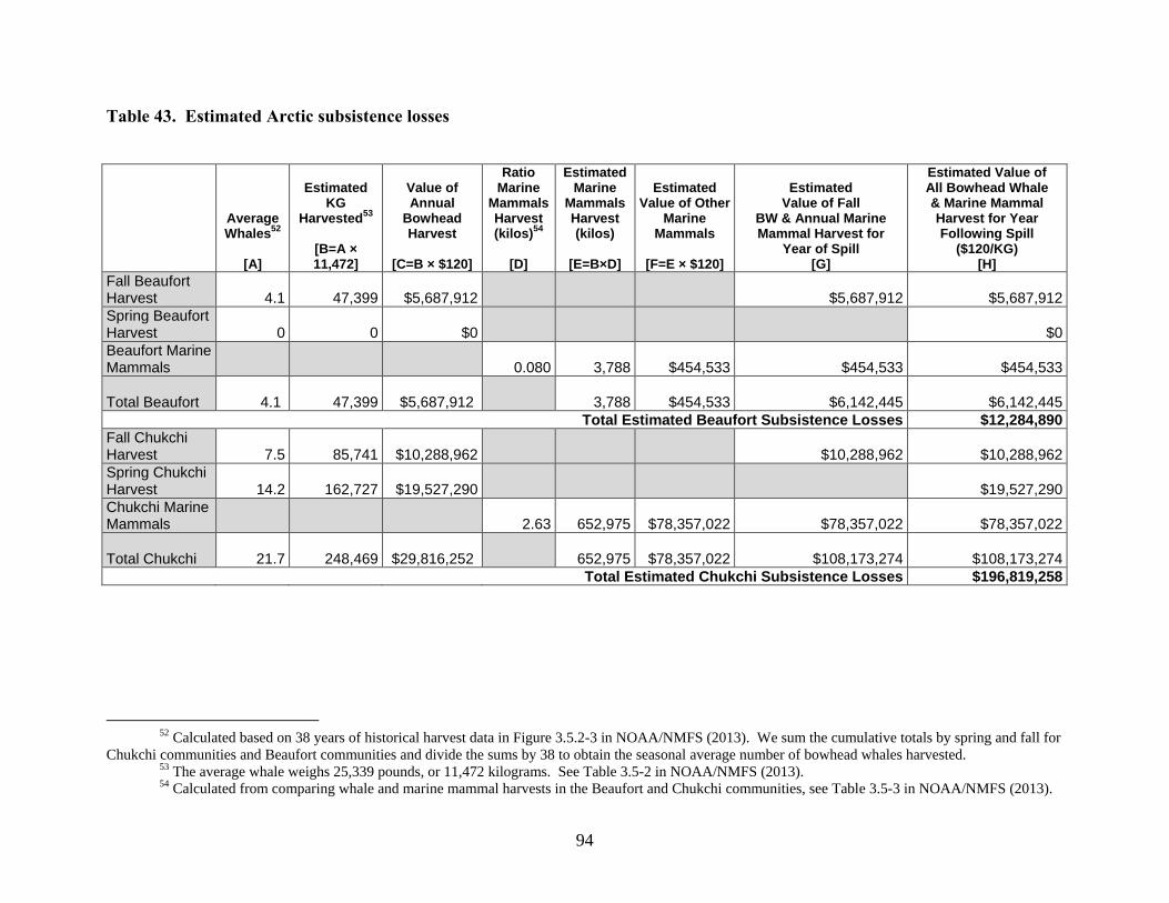
94

Table 43. Estimated Arctic subsistence losses

Average Whales

52

[A]

Estimated KG

Harvested53

[B=A × 11,472]

Value of Annual

Bowhead Harvest

[C=B × $120]

Ratio Marine

Mammals Harvest (kilos)

54

[D]

Estimated Marine

Mammals Harvest (kilos)

[E=B×D]

Estimated Value of Other

Marine Mammals

[F=E × $120]

Estimated Value of Fall

BW & Annual Marine Mammal Harvest for

Year of Spill [G]

Estimated Value of All Bowhead Whale & Marine Mammal Harvest for Year Following Spill

($120/KG) [H]

Fall Beaufort Harvest 4.1

47,399 $5,687,912

$5,687,912 $5,687,912

Spring Beaufort Harvest 0

0 $0 $0

Beaufort Marine Mammals 0.080

3,788 $454,533 $454,533 $454,533

Total Beaufort 4.1

47,399 $5,687,912

3,788 $454,533 $6,142,445 $6,142,445

Total Estimated Beaufort Subsistence Losses $12,284,890

Fall Chukchi Harvest 7.5

85,741 $10,288,962 $10,288,962 $10,288,962

Spring Chukchi Harvest 14.2

162,727 $19,527,290 $19,527,290

Chukchi Marine Mammals 2.63

652,975 $78,357,022 $78,357,022 $78,357,022

Total Chukchi 21.7

248,469 $29,816,252

652,975 $78,357,022 $108,173,274 $108,173,274

Total Estimated Chukchi Subsistence Losses $196,819,258

52 Calculated based on 38 years of historical harvest data in Figure 3.5.2-3 in NOAA/NMFS (2013). We sum the cumulative totals by spring and fall for

Chukchi communities and Beaufort communities and divide the sums by 38 to obtain the seasonal average number of bowhead whales harvested. 53 The average whale weighs 25,339 pounds, or 11,472 kilograms. See Table 3.5-2 in NOAA/NMFS (2013). 54 Calculated from comparing whale and marine mammal harvests in the Beaufort and Chukchi communities, see Table 3.5-3 in NOAA/NMFS (2013).

95

3.6 FATAL AND NONFATAL INJURIES

CDEs may unfortunately cause serious injuries or fatalities to individuals located near the well.

To estimate the costs associated with the loss of life and nonfatal injuries associated with a CDE,

we draw upon the historical experience of the two well blowout events in the U.S. that led to

fatalities. The first, which occurred in 1984, caused four fatalities and three non-fatal injuries.

The second, the Deepwater Horizon blowout in 2010, resulted in 11 fatalities and 17 non-fatal

injuries.55

For the purposes of estimating the impacts of a potential CDE in the future, we

average the fatalities and non-fatal injuries across these two events. This results in an average of

eight fatalities and ten non-fatal injuries per incident.

We estimate the economic value of fatalities based on the value of a statistical life (VSL).

Drawing from the U.S. EPA’s meta-analysis of the VSL literature, we estimate that the VSL in

year 2017 dollars and at year 2017 income levels is approximately $9.5 million.56

The

adjustment for income reflects a VSL elasticity with respect to income (i.e., the percent change

in VSL due to one percent change in income) of 0.4, consistent with the value from Kleckner and

Neumann (1999) used in EPA regulatory impact analyses. Based on the estimated value of eight

deaths per incident and the VSL of $9.5 million, the total cost of fatalities due to a CDE is

estimated to be $75.8 million (in year 2017$).

Viscusi (2005) estimates that workers place a value on non-fatal injuries that ranges from

$20,000 to $70,000 per expected job injury.57

Using the midpoint of this range ($45,000), and

inflating it to year 2017 dollars, we estimate a value of $57,100 per injury. Applying this value

to the assumed ten injuries per incident, we estimate costs of approximately $571,000 associated

with non-fatal injuries resulting from a CDE. Summing this with the $75.8 million associated

with CDE-related fatalities, we estimate $76.4 million in damages associated with fatalities and

non-fatal injuries. Because a blowout resulting in these impacts would result in spills ranging

substantially with respect to the volume of oil spilled, we do not estimate the value of fatal and

non-fatal injuries on a per-barrel basis.

3.7 VALUE OF SPILLED OIL NOT RECOVERED

Another cost associated with a CDE is the value of spilled oil not recovered. Recognizing that

the dollar per barrel value of oil is highly unpredictable and will vary over time and that the

timing of a CDE is highly uncertain, we estimate the value of spilled oil using the oil prices

associated with BOEM’s Low, Mid-, and High Oil Price E&D scenarios. These values are $40,

$100, and $160 per barrel, respectively.

55 See BOEMRE (2010). 56 See U.S. EPA (2014). 57 See Viscusi (2005).

96

3.8 IMPACTS OF DISPERSANTS AND IN-SITU BURNS

While dispersants and in-situ burns can be effective oil spill response strategies, they also have

potential environmental costs. In-situ burns produce large amounts of smoke, which contains

particulate matter and air pollutants such as sulfur dioxide, nitrogen dioxide, and carbon

monoxide. These pollutants have the potential to negatively impact the health of response

workers and residents of nearby coastal areas. PM—from direct PM emissions or from precursor

emissions that transform into PM—presents the greatest concern, as studies have demonstrated

that concentrations of particulate matter within the smoke plume can remain above background

levels several miles downwind of the burn site. In-situ burns also have the potential to damage

vegetation in coastal areas, and leave behind an oil residue that can sink and smother benthic

resources under certain conditions (Barnea, 1995).

Dispersants can reduce oil exposure for surface dwelling organisms, and prevent oil from

reaching the shoreline habitat. However, these benefits come with the tradeoff of distributing oil

throughout the water column and into the benthic environment. Even in a diluted form, exposure

to dispersed oil can cause injury to fish, oysters, coral reefs, and other subsurface ecological

resources. As a result, the net ecological impact of dispersant usage is necessarily dependent on

the relative vulnerability of surface and subsurface habitats in a given location (NRC, 2005). The

ecological impacts of the chemical dispersants themselves are not as large of a concern, as the

dispersants in use today are generally less toxic than the dispersed oil. Research on dispersant

use during the Deepwater Horizon spill confirmed this lower toxicity, finding that dispersant-oil

mixtures were generally no more harmful to aquatic species than oil alone (EPA, 2010).

3.9 UNCERTAINTIES

Due to the various assumptions and limitations of the available data described in the previous

sections, the CDE damage estimates presented throughout this chapter exhibit substantial

uncertainty. Table 44 documents the most significant of these uncertainties and describes their

potential impact on our estimates of CDE-related damages.

97

Table 44. Uncertainties, limitations, and assumptions of analysis

Impact Category Uncertainties, Limitations, and Assumptions Implications for Impact Estimates

Response Costs

We assume that the response costs for the Deepwater Horizon spill are representative of response costs for CDEs occurring in the Gulf of Mexico.

Assumption could lead to overestimation or underestimation of impacts, depending on the timing and location of a CDE and conditions when the CDE occurs (e.g., currents and wind direction).

We assume that response costs in the Atlantic are the same as those in the Gulf of Mexico.

Because wetlands are less prevalent on the Atlantic shoreline, we may overestimate response costs for the Atlantic.

We assume that the response costs for the Exxon Valdez spill are representative of response costs for CDEs occurring in Cook Inlet.

Assumption could lead to overestimation or underestimation of impacts, depending on how the timing, size, and duration of a CDE in Cook Inlet differ from the experience of the Exxon Valdez spill in Prince William Sound.

We assume that a CDE in the Atlantic Program Area would affect shoreline in the states whose waters are adjacent to the Mid-Atlantic OCS Planning Area.

Assumption could lead to overestimation of impacts, depending on the location of a CDE and conditions when the CDE occurs. If oil from a CDE flows to the North Atlantic or South Atlantic, response costs may be lower due to the higher proportion of beaches and lower proportion of wetlands in these regions.

We assume that response costs for a CDE in the Arctic will be greater than or equal to the response costs for the Deepwater Horizon spill ($5,100/barrel) and less than or equal to the response costs for the Exxon Valdez spill ($16,000/barrel).

Assumption could lead to overestimation or underestimation of impacts, depending on the location of a CDE and conditions when the CDE occurs

Ecological Damages

We assume that the ecological damages for the Deepwater Horizon spill are representative of ecological damages for CDEs occurring in the Gulf of Mexico.

Assumption could lead to overestimation or underestimation of impacts, depending on the timing and location of a CDE and conditions when the CDE occurs (e.g., currents and wind direction).

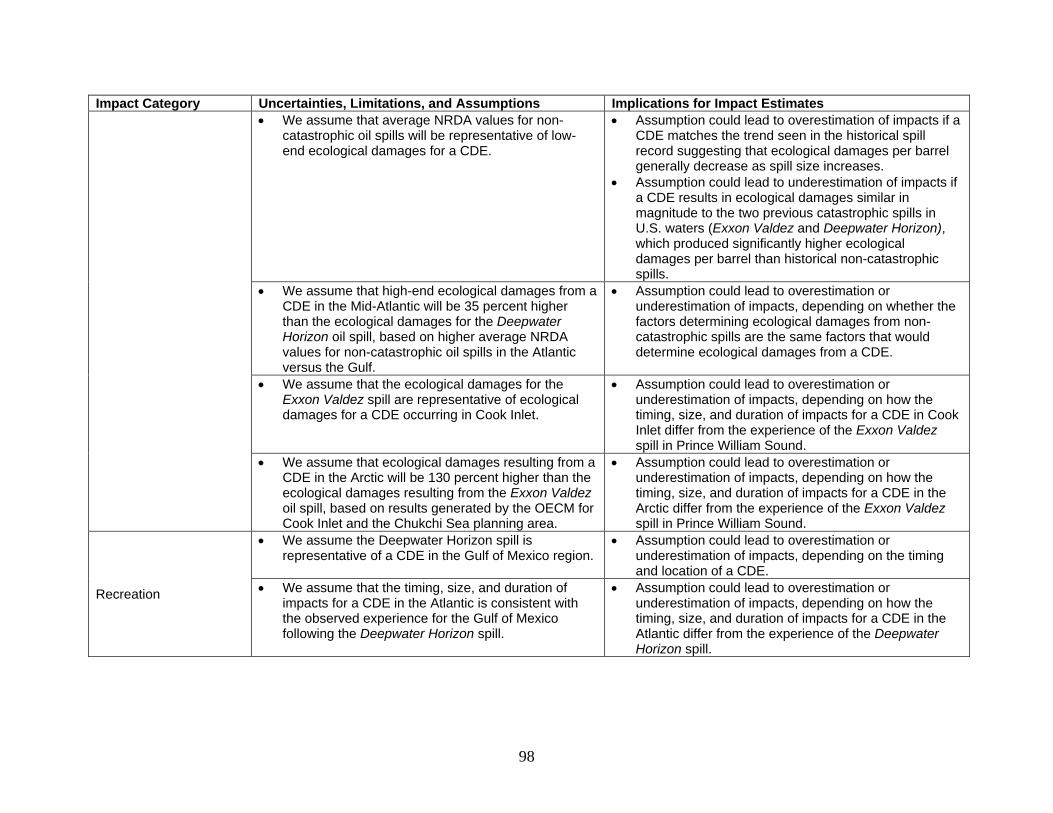
98


We assume that average NRDA values for non-catastrophic oil spills will be representative of low-end ecological damages for a CDE.

Assumption could lead to overestimation of impacts if a CDE matches the trend seen in the historical spill record suggesting that ecological damages per barrel generally decrease as spill size increases.

Assumption could lead to underestimation of impacts if a CDE results in ecological damages similar in magnitude to the two previous catastrophic spills in U.S. waters (Exxon Valdez and Deepwater Horizon), which produced significantly higher ecological damages per barrel than historical non-catastrophic spills.

We assume that high-end ecological damages from a CDE in the Mid-Atlantic will be 35 percent higher than the ecological damages for the Deepwater Horizon oil spill, based on higher average NRDA values for non-catastrophic oil spills in the Atlantic versus the Gulf.

Assumption could lead to overestimation or underestimation of impacts, depending on whether the factors determining ecological damages from non-catastrophic spills are the same factors that would determine ecological damages from a CDE.

We assume that the ecological damages for the Exxon Valdez spill are representative of ecological damages for a CDE occurring in Cook Inlet.

Assumption could lead to overestimation or underestimation of impacts, depending on how the timing, size, and duration of impacts for a CDE in Cook Inlet differ from the experience of the Exxon Valdez spill in Prince William Sound.

We assume that ecological damages resulting from a CDE in the Arctic will be 130 percent higher than the ecological damages resulting from the Exxon Valdez oil spill, based on results generated by the OECM for Cook Inlet and the Chukchi Sea planning area.

Assumption could lead to overestimation or underestimation of impacts, depending on how the timing, size, and duration of impacts for a CDE in the Arctic differ from the experience of the Exxon Valdez spill in Prince William Sound.

Recreation

We assume the Deepwater Horizon spill is representative of a CDE in the Gulf of Mexico region.

Assumption could lead to overestimation or underestimation of impacts, depending on the timing and location of a CDE.

We assume that the timing, size, and duration of impacts for a CDE in the Atlantic is consistent with the observed experience for the Gulf of Mexico following the Deepwater Horizon spill.

Assumption could lead to overestimation or underestimation of impacts, depending on how the timing, size, and duration of impacts for a CDE in the Atlantic differ from the experience of the Deepwater Horizon spill.

99


We assume that a CDE in the Atlantic would affect recreation in the states near the Mid-Atlantic OCS Planning Area.

Assumption could lead to overestimation or underestimation of impacts, depending on the location of a CDE and conditions when the CDE occurs. For example, oil from a CDE could spread up the coast to the North Atlantic, impacting New Jersey. Alternatively, the oil from a CDE on the Atlantic could drift into the open ocean away from the coast.

Our quantitative assessment of potential recreational impacts in the Atlantic does not include boating impacts.

Likely leads to slight underestimation of impacts. Based on the experience of the Deepwater Horizon spill, however, boating impacts are small relative to beach use and coastal fishing.

The 2000 NSRE data used to derive baseline beach use in the Atlantic are fairly outdated.

Use of these data could lead to overestimation or underestimation of use, depending on the trajectory of use since 2000.

We assume that the reduction in recreational fishing observed in south-central Alaska following the Exxon Valdez spill would also apply to recreational fishing in Cook Inlet.

Assumption could lead to overestimation or underestimation of impacts, depending on amount of oiling relative to the Valdez spill and the timing of a CDE relative to the timing of Valdez.

For recreational fishing in Cook Inlet, we assume a CDE volume equal to that of the Exxon Valdez spill to calculate damages on a per barrel basis.

Assumption could lead to overestimation or underestimation of impacts depending on damages per barrel for future CDEs relative to damages per barrel for the Valdez spill.

In the absence of wildlife viewing data specific to Cook Inlet, we used data for southcentral Alaska as a whole.

Likely leads to overestimation of wildlife viewing impacts since not all wildlife viewing in southcentral Alaska is in Cook Inlet.

Consistent with BOEM’s 2012 analysis of catastrophic spill impacts, we assume a high-impact spill scenario for wildlife viewing in Cook Inlet in which a CDE occurs in the summer and last for 80 days, which represents 53 percent of the summer season.

Assumption could lead to overestimation of impacts if a CDE occurs during another time of the year.

To estimate the economic value of Cook Inlet wildlife viewing losses, we assume that half of the value of a wildlife viewing day will be lost for affected trips.

Assumption could lead to overestimation or underestimation of impacts, depending on the extent to which recreators change their wildlife viewing behavior in response to a CDE.

100


Subsistence

Information on baseline subsistence harvests, estimates of the change in subsistence associated with a CDE, and an economic value of lost subsistence is limited.

Because these data are so limited, our estimates of subsistence impacts are highly uncertain and may be overestimates or underestimates.

Economic valuation methods are ill-suited to quantifying the cultural value of subsistence for Native Alaskan communities.

Value of subsistence to Native Alaska communities may be underestimated.

We assume that the reduction in subsistence observed in south-central Alaska following the Exxon Valdez spill would also apply to subsistence in the Artic.

Assumption could lead to overestimation or underestimation of subsistence impacts depending on the extent to which future CDEs affect the level of subsistence relative to the impacts of the Valdez spill.

For subsistence in Cook Inlet, we use the spill volume from the Exxon Valdez spill to calculate damages on a per barrel basis.

Assumption could lead to overestimation or underestimation of impacts depending on damages per barrel for future CDE relative to damages per barrel for the Valdez spill.

In the Artic, consistent with BOEM (2012), we assume that the fall bowhead whale hunt and marine mammal harvest are lost in the year of a catastrophic spill and that both the spring and fall harvests are lost the following year.

Assumption could lead to overestimation or underestimation of subsistence impacts depending on the extent to which future CDEs affect subsistence harvests.

Fatal and Nonfatal Injuries

Our estimate of the number of fatalities associated with a CDE is based only on two data points: a blowout in 1984 spill and the Deepwater Horizon blowout in 2010.

Assumption could lead to overestimation or underestimation of the number of fatalities associated with a CDE. The actual number is likely to vary depending on the cause of the spill and the number of people aboard a platform during a CDE.

Value of Oil Spilled We assume a range of oil price values based on the

low and high price assumptions that inform BOEM’s low and high E&D scenarios.

Given the wide range of oil prices used, impacts are most likely within the range estimated.

101

3.10 REFERENCES

Alaska Department of Fish and Game (ADFG) (2014), Alaska Commercial Salmon Harvests and

Exvessel Values, available at

http://www.adfg.alaska.gov/index.cfm%3Fadfg%3DCommercialByFisherySalmon.exves

selquery

Alaska Department of Fish and Game (ADFG) (2013), “Alaska Sport Fishing Survey”

Southcentral Alaska Region, (PS) Cook Inlet saltwater, Harvest Estimates.

https://www.adfg.alaska.gov/sf/sportfishingsurvey/index.cfm?ADFG=main.home

Alaska Department of Fish and Game (ADFG), Division of Subsistence (2014), “Subsistence in

Alaska: A Year 2012 Update”.

http://www.adfg.alaska.gov/static/home/subsistence/pdfs/subsistence_update_2012.pdf

Alaska Department of Fish and Game (ADFG), Division of Subsistence (2015), “Community

Subsistence Information System (CSIS)”.

http://www.adfg.alaska.gov/sb/CSIS/index.cfm?ADFG=main.home

Alaska Department of Fish and Game (ADFG), Exxon Valdez Oil Spill Trustee Council,

"Questions and Answers". http://www.evostc.state.ak.us/index.cfm?FA=facts.QA

Alaska Department of Labor and Workforce Development (ADLWD) (2010), “2010 Census

Demographic Profiles”. Research and Analysis.

http://live.laborstats.alaska.gov/cen/dparea.cfm

Barnea, Nir, (1995), “Health and safety aspects of in-situ burning of oil.” Report to National

Oceanic and Atmospheric Administration, Seattle, WA.

Bell, F. and Leeworthy, V., (1986), “An Economic Analysis of the Importance of Saltwater

Beaches in Florida” Florida Sea Grant Report 82, pp. 1-166. Gainesville, University of

Florida.

Bell F., and Leeworthy V.R. (1990), "Recreational demand by tourists for saltwater beach days".

Journal of Environmental Economics and Management 18(3): 189-205.

Bergstrom, J.C, Dorfman, J., and Loomis, J.B., (2004) “Estuary Management and Recreational

Fishing Benefits” Coastal Management, 32:417–432.

Bin et al. (2004), “Some Consumer Surplus Estimates for North Carolina Beaches.”

Blomo, V.J., J.P. Nichols, W.L. Griffin and W.E. Grant, (1982). “Dynamic Modeling of the

Eastern Gulf of Mexico Shrimp Fishery,” American Journal of Agricultural Economics,

64: 475-482.

BOEMRE, (2010), “Benefit-Cost Analysis for the Interim Final Rule on Increased Safety

Measures for Energy Development on the Outer Continental Shelf.”

Bouchard B-120 Oil Spill Lost Use Technical Working Group. (2009). Bouchard B-120 Oil Spill

Buzzards Bay, Massachusetts, Lost Use Valuation Report.

BP, (2015), “Gulf of Mexico Environmental Recovery and Restoration Five Year Report.”

http://www.adfg.alaska.gov/index.cfm%3Fadfg%3DCommercialByFisherySalmon.exvesselquery

http://www.adfg.alaska.gov/index.cfm%3Fadfg%3DCommercialByFisherySalmon.exvesselquery

https://www.adfg.alaska.gov/sf/sportfishingsurvey/index.cfm?ADFG=main.home

http://www.adfg.alaska.gov/static/home/subsistence/pdfs/subsistence_update_2012.pdf

http://www.adfg.alaska.gov/sb/CSIS/index.cfm?ADFG=main.home

http://www.evostc.state.ak.us/index.cfm?FA=facts.QA

http://live.laborstats.alaska.gov/cen/dparea.cfm

102

Commonwealth of Pennsylvania Department of Environmental Protection, (1995), “RE: M/T

Kentucky; Paulsboro NJ Oil Spill July 22-24, 1994.”

Downing, M., and Ozuna, T., (1996), "Testing the Reliability of the Benefit Function Transfer

Approach". Journal of Environmental Economics and Management 30, 316-322.

Etkin, Dagmar Schmidt, (1999), "Estimating cleanup costs for oil spills." International Oil Spill

Conference. Vol. 1999. No. 1. American Petroleum Institute.

Etkin, Dagmar Schmidt, (2000), "Worldwide analysis of marine oil spill cleanup cost

factors." Arctic and marine oil spill program technical seminar. Vol. 1. Environment

Canada.

Etkin, Dagmar Schmidt, (2004), "Modeling oil spill response and damage costs." Proceedings of

the Fifth Biennial Freshwater Spills Symposium.

Florida Department of Environmental Protection, National Oceanic and Atmospheric

Administration, and U.S. Department of the Interior, (1997), “Damage Assessment and

Restoration Plan/ Environmental Assessment for the August 10, 1993 Tampa Bay Oil

Spill.”

Hamel, C. Herrmann, M.Lee, S.T.Criddle, K.R. (2000), “An Economic Discussion of Marine

Sport Fisheries in Central and Lower Cook Inlet.”

Hausman, J.A., Leonard, G.K., and McFadden D., (1995), "A utility consistent, combined

discrete choise and count data model; assessing recreational use losses due to natural

resource damage." Journal of Public Economics 56, 1-30.

Houston, J.E., A.E. Nieto, J.E. Epperson, Ho-Shui Li and G.W. Lewis, (1989), “Factors

Affecting Local Prices of Shrimp Landings,” Marine Resource Economics, 6: 163-72.

Industrial Economics, Inc.; Applied Science Associates, Inc.; Northern Economics; and Dr.

Nicholas Z. Muller. 2012a. Forecasting Environmental and Social Externalities

Associated with OCS Oil and Gas Development: The Revised Offshore Environmental

Cost Model (OECM) (BOEM 2012-025). U.S. Department of the Interior, Bureau of

Ocean Energy Management.

Kleckner, N., and J. Neumann. 1999. Recommended Approach to Adjusting WTP Estimates to

Reflect Changes in Real Income. Memorandum to Jim DeMocker, U.S. EPA/OPAR.

June 3. Available at

<http://www.epa.gov/ttn/ecas/regdata/Benefits/background/klecknerandneumann1999.pd

f>.

English, E. (2015) “BC-1 - Early Data Collection,” technical memorandum submitted to Craig

O’Connor of NOAA in support of the Deepwater Horizon Preliminary Damage

Assessment and Restoration Plan.

English, E. (2015). “BC-2 - Supplemental Shoreline Adjustment,” technical memorandum

submitted to Craig O’Connor of NOAA in support of the Deepwater Horizon Preliminary

Damage Assessment and Restoration Plan.

English, E. and K. McConnell. (2015). “A - Overview of Recreation Assessment,” technical

memorandum submitted to Craig O’Connor of NOAA in support of the Deepwater

Horizon Preliminary Damage Assessment and Restoration Plan.

103

Federal Reserve Bank of St. Louis, Economic Research Division “Federal Reserve Economic

Data”. https://research.stlouisfed.org/fred2/

Leeworthy, V.R. and Bowker, J.M. (1997), "Nonmarket Economic User Values of the Florida

Keys/Key West". National Oceanic and Atmospheric Administration (NOAA), National

Ocean Service (NOS), Forest Service, Outdoor Recreation and Wilderness Assessment

Group.

Leeworthy, V.R., and P.C. Wiley (2001), “Current Participation Patterns in Marine Recreation”,

Beach Visitation by State in Which Beach is Located. U.S. Department of Commerce,

National Oceanic and Atmospheric Administration, National Ocean Service Special

Projects- Silver Spring, Maryland.

Leeworthy, V.R., and P.C Wiley (1994), “Recreational use value for Clearwater Beach and

Honeymoon Island State Park, Florida” National Oceanic and Atmospheric

Administration (NOAA).

Leeworthy, V.R. P.C. Wiley (1991) “Recreational use value for Island Beach State Park”

National Oceanic and Atmospheric Administration (NOAA), Strategic Environmental

Assessments Division, Office of Ocean Resources and Conservation.

McConnell, Kenneth. (2015). “I5 - Adjustment for Undercoverage of Nighttime Fishing,”

technical memorandum submitted to Craig O’Connor of NOAA in support of the

Deepwater Horizon Preliminary Damage Assessment and Restoration Plan.

McConnell K.E., and I.E. Strand (1994), "The Economic Value of Mid and South Atlantic

Sportfishing" University of Maryland, College Park.

McDowell Group (2011), “Alaska Visitor Statistics Program VI Summer 2011” prepared for

Alaska Department of Commerce, Community, & Economic Development Division of

Economic Development.

McDowell Group (2014), “Alaska Visitor Statistics Program VI Interim Visitor Volume Report

Summer 2014” Chart 4, “Summer Visitor Volume to Alaska 2005-2014” prepared for

Alaska Department of Commerce, Community and Economic Development, Division of

Economic Development.

https://www.commerce.alaska.gov/web/Portals/6/pub/TourismResearch/AVSP/2013_201

4/AVSP%20VI%20Summer%202014%20FINAL.pdf

Mills, Michael J. (1992), “Alaska Sport Fishing in the Aftermath of the Exxon Valdez Oil Spill,

Special Publication No. 92-5”, prepared for Alaska Department of Fish and Game.

December 1992.

Montauk Oil Transportation Corp. v. Steamship Mutual Underwriting Association (Bermuda),

Limited. Consent Decree. 90 Civil No. 5702 (KMW). United States District Court

Southern District of New York. December 1998. http://www.gc.noaa.gov/gc-cd/cibro-

a.pdf

National Research Council (2005), “Oil Spill Dispersants: Efficacy and Effects.” Washington,

DC: The National Academies Press.

https://research.stlouisfed.org/fred2/

https://www.commerce.alaska.gov/web/Portals/6/pub/TourismResearch/AVSP/2013_2014/AVSP%20VI%20Summer%202014%20FINAL.pdf

https://www.commerce.alaska.gov/web/Portals/6/pub/TourismResearch/AVSP/2013_2014/AVSP%20VI%20Summer%202014%20FINAL.pdf

http://www.gc.noaa.gov/gc-cd/cibro-a.pdf

http://www.gc.noaa.gov/gc-cd/cibro-a.pdf

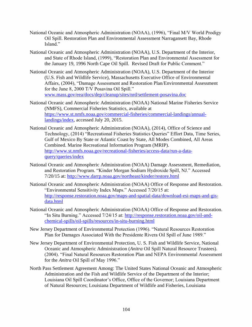
104

National Oceanic and Atmospheric Administration (NOAA), (1996), “Final M/V World Prodigy

Oil Spill. Restoration Plan and Environmental Assessment Narragansett Bay, Rhode

Island.”

National Oceanic and Atmospheric Administration (NOAA), U.S. Department of the Interior,

and State of Rhode Island, (1999), “Restoration Plan and Environmental Assessment for

the January 19, 1996 North Cape Oil Spill. Revised Draft for Public Comment.”

National Oceanic and Atmospheric Administration (NOAA), U.S. Department of the Interior

(U.S. Fish and Wildlife Service), Massachusetts Executive Office of Environmental

Affairs, (2004), “Damage Assessment and Restoration Plan/Environmental Assessment

for the June 8, 2000 T/V Posavina Oil Spill.”

www.mass.gov/eea/docs/dep/cleanup/sites/nrd/settlement-posavina.doc

National Oceanic and Atmospheric Administration (NOAA) National Marine Fisheries Service

(NMFS), Commercial Fisheries Statistics, available at

https://www.st.nmfs.noaa.gov/commercial-fisheries/commercial-landings/annual-

landings/index, accessed July 20, 2015.

National Oceanic and Atmospheric Administration (NOAA), (2014), Office of Science and

Technology, (2014) “Recreational Fisheries Statistics Queries” Effort Data, Time Series,

Gulf of Mexico By State or Atlantic Coast by State, All Modes Combined, All Areas

Combined. Marine Recreational Information Program (MRIP).

http://www.st.nmfs.noaa.gov/recreational-fisheries/access-data/run-a-data-

query/queries/index

National Oceanic and Atmospheric Administration (NOAA) Damage Assessment, Remediation,

and Restoration Program. “Kinder Morgan Sodium Hydroxide Spill, NJ.” Accessed

7/20/15 at: http://www.darrp.noaa.gov/northeast/kinder/restore.html

National Oceanic and Atmospheric Administration (NOAA) Office of Response and Restoration.

“Environmental Sensitivity Index Maps.” Accessed 7/20/15 at:

http://response.restoration.noaa.gov/maps-and-spatial-data/download-esi-maps-and-gis-

data.html

National Oceanic and Atmospheric Administration (NOAA) Office of Response and Restoration.

“In Situ Burning.” Accessed 7/24/15 at: http://response.restoration.noaa.gov/oil-and-

chemical-spills/oil-spills/resources/in-situ-burning.html

New Jersey Department of Environmental Protection (1996). “Natural Resources Restoration

Plan for Damages Associated With the Presidente Rivera Oil Spill of June 1989.”

New Jersey Department of Environmental Protection, U. S. Fish and Wildlife Service, National

Oceanic and Atmospheric Administration (Anitra Oil Spill Natural Resource Trustees).

(2004). “Final Natural Resources Restoration Plan and NEPA Environmental Assessment

for the Anitra Oil Spill of May 1996.”

North Pass Settlement Agreement Among: The United States National Oceanic and Atmospheric

Administration and the Fish and Wildlife Service of the Department of the Interior;

Louisiana Oil Spill Coordinator’s Office, Office of the Governor; Louisiana Department

of Natural Resources; Louisiana Department of Wildlife and Fisheries, Louisiana

https://www.st.nmfs.noaa.gov/commercial-fisheries/commercial-landings/annual-landings/index

https://www.st.nmfs.noaa.gov/commercial-fisheries/commercial-landings/annual-landings/index

http://www.st.nmfs.noaa.gov/recreational-fisheries/access-data/run-a-data-query/queries/index

http://www.st.nmfs.noaa.gov/recreational-fisheries/access-data/run-a-data-query/queries/index

http://www.darrp.noaa.gov/northeast/kinder/restore.html



http://response.restoration.noaa.gov/oil-and-chemical-spills/oil-spills/resources/in-situ-burning.html

http://response.restoration.noaa.gov/oil-and-chemical-spills/oil-spills/resources/in-situ-burning.html

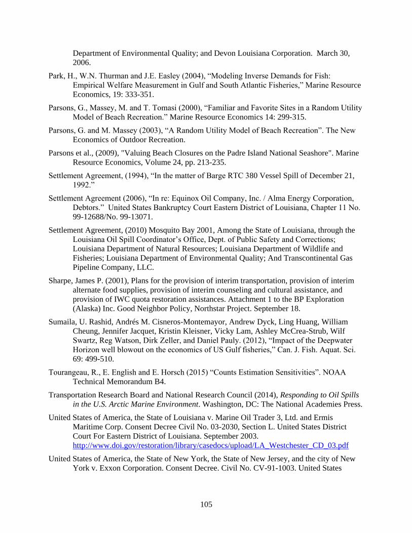
105

Department of Environmental Quality; and Devon Louisiana Corporation. March 30,

2006.

Park, H., W.N. Thurman and J.E. Easley (2004), “Modeling Inverse Demands for Fish:

Empirical Welfare Measurement in Gulf and South Atlantic Fisheries,” Marine Resource

Economics, 19: 333-351.

Parsons, G., Massey, M. and T. Tomasi (2000), “Familiar and Favorite Sites in a Random Utility

Model of Beach Recreation.” Marine Resource Economics 14: 299-315.

Parsons, G. and M. Massey (2003), “A Random Utility Model of Beach Recreation”. The New

Economics of Outdoor Recreation.

Parsons et al., (2009), "Valuing Beach Closures on the Padre Island National Seashore". Marine

Resource Economics, Volume 24, pp. 213-235.

Settlement Agreement, (1994), “In the matter of Barge RTC 380 Vessel Spill of December 21,

1992.”

Settlement Agreement (2006), “In re: Equinox Oil Company, Inc. / Alma Energy Corporation,

Debtors.” United States Bankruptcy Court Eastern District of Louisiana, Chapter 11 No.

99-12688/No. 99-13071.

Settlement Agreement, (2010) Mosquito Bay 2001, Among the State of Louisiana, through the

Louisiana Oil Spill Coordinator’s Office, Dept. of Public Safety and Corrections;

Louisiana Department of Natural Resources; Louisiana Department of Wildlife and

Fisheries; Louisiana Department of Environmental Quality; And Transcontinental Gas

Pipeline Company, LLC.

Sharpe, James P. (2001), Plans for the provision of interim transportation, provision of interim

alternate food supplies, provision of interim counseling and cultural assistance, and

provision of IWC quota restoration assistances. Attachment 1 to the BP Exploration

(Alaska) Inc. Good Neighbor Policy, Northstar Project. September 18.

Sumaila, U. Rashid, Andrés M. Cisneros-Montemayor, Andrew Dyck, Ling Huang, William

Cheung, Jennifer Jacquet, Kristin Kleisner, Vicky Lam, Ashley McCrea-Strub, Wilf

Swartz, Reg Watson, Dirk Zeller, and Daniel Pauly. (2012), “Impact of the Deepwater

Horizon well blowout on the economics of US Gulf fisheries,” Can. J. Fish. Aquat. Sci.

69: 499-510.

Tourangeau, R., E. English and E. Horsch (2015) “Counts Estimation Sensitivities”. NOAA

Technical Memorandum B4.

Transportation Research Board and National Research Council (2014), Responding to Oil Spills

in the U.S. Arctic Marine Environment. Washington, DC: The National Academies Press.

United States of America, the State of Louisiana v. Marine Oil Trader 3, Ltd. and Ermis

Maritime Corp. Consent Decree Civil No. 03-2030, Section L. United States District

Court For Eastern District of Louisiana. September 2003.

http://www.doi.gov/restoration/library/casedocs/upload/LA_Westchester_CD_03.pdf

United States of America, the State of New York, the State of New Jersey, and the city of New

York v. Exxon Corporation. Consent Decree. Civil No. CV-91-1003. United States

http://www.doi.gov/restoration/library/casedocs/upload/LA_Westchester_CD_03.pdf

106

District Court For the Eastern District of New York. March 1991.

http://www.gc.noaa.gov/gc-cd/exx2.pdf.

United States of America, the State of New York, the State of New Jersey, and the city of New

York v. Nautilus Motor Tanker Co., Ltd. Consent Decree. Civil No. 90-cv-24-WGB.

United States District Court For the District of New Jersey. April 1994.

http://www.gc.noaa.gov/gc-cd/nautilis.pdf.

United States of America, Commonwealth of Massachusetts, and the State of Rhode Island v.

Bouchard Transportation Company, Inc., Tug Evening Tide Corporation, and B. No 120

Corporation. Consent Decree. Civil No. 1:10-cv-11958-NMG. United States District

Court District of Massachusetts. May 2011. http://www.gc.noaa.gov/gc-cd/051911-cb-

bouchard.pdf

United States of America and the State of Maine v. Amity Products Carriers, Inc. Consent

Decree. Civil No. 00-11-P-H and 00-12-P-H. United States District Court For the District

of Maine. May 2000. http://www.gc.noaa.gov/gc-cd/julien-cd.pdf

U.S. Census Bureau (2015), “Geography Area Series: County Business Patterns, 2013 Business

Patterns”. All Florida Counties, NAICS code 721.

http://factfinder.census.gov/faces/tableservices/jsf/pages/productview.xhtml?pid=BP_201

3_00A1&prodType=table

U.S. Department of Commerce, National Oceanic and Atmospheric Administration (NOAA)

(2015) Deepwater Horizon Response and Restoration: Administrative Record.

U.S. Department of Commerce, National Oceanic and Atmospheric Administration (NOAA)

(2015) “Deepwater Horizon Draft Programmatic Damage Assessment and Restoration

Plan” Chapter 4: Injury to Natural Resources – Section 4: Lost Human Use, 4.10: Lost

Recreational Use.

U.S. Department of Commerce, National Oceanic and Atmospheric Administration (NOAA),

National Marine Fisheries Service (2013), “Final Environmental Impact Statement for

Issuing Annual Quotas to the Alaska Eskimo Whaling Commission for a Subsistence

Hunt on Bowhead Whales for the Years 2013 through 2018.”

https://alaskafisheries.noaa.gov/protectedresources/whales/bowhead/eis0113/final.pdf

U.S. Department of Justice (DOJ), (2015), Statement by Attorney General Loretta E. Lynch on

the Agreement in Principle with BP to Settle Civil Claims for the Deepwater Horizon Oil

Spill. http://www.justice.gov/opa/pr/statement-attorney-general-loretta-e-lynch-

agreement-principle-bp-settle-civil-claims.

U.S. Department of the Interior, Bureau of Ocean Energy Management (BOEM) (2015), “2017-

2022 Outer Continental Shelf Oil and Gas Leasing Draft Proposed Program”.

U.S. Department of the Interior. Bureau of Ocean Energy Management Regulation and

Enforcement (BOEMRE) (2010), “Regulatory Impact Analysis for the Drilling Safety

Rule, RIN1010 AD68.”

U.S. Department of the Interior, Bureau of Ocean Energy Management (BOEM) (2012),

“Economic Analysis Methodology for the Five Year OCS Oil and Gas Leasing Program

for 2012-2017”.

http://www.gc.noaa.gov/gc-cd/exx2.pdf

http://www.gc.noaa.gov/gc-cd/nautilis.pdf

http://www.gc.noaa.gov/gc-cd/051911-cb-bouchard.pdf

http://www.gc.noaa.gov/gc-cd/051911-cb-bouchard.pdf

http://www.gc.noaa.gov/gc-cd/julien-cd.pdf

http://factfinder.census.gov/faces/tableservices/jsf/pages/productview.xhtml?pid=BP_2013_00A1&prodType=table

http://factfinder.census.gov/faces/tableservices/jsf/pages/productview.xhtml?pid=BP_2013_00A1&prodType=table

https://alaskafisheries.noaa.gov/protectedresources/whales/bowhead/eis0113/final.pdf

http://www.justice.gov/opa/pr/statement-attorney-general-loretta-e-lynch-agreement-principle-bp-settle-civil-claims

http://www.justice.gov/opa/pr/statement-attorney-general-loretta-e-lynch-agreement-principle-bp-settle-civil-claims

107

U.S. Department of the Interior. Minerals Management Service (MMS) (2001), “Long-Term

Consequences of the Exxon Valdez Oil Spill for Coastal Communities of Southcentral

Alaska” (MMS 2001-032). www.alaska.boemre.gov/reports/2001rpts/2001_032.pdf

U.S. Department of the Interior, National Park Service (NPS) (2014), National Seashores:

“Recreation Visitors by Month (1979-Last Calendar Year)”. National Park Visitor Use

Statistics. https://irma.nps.gov/Stats/

U.S. Department of Labor, Bureau of Labor Statistics (BLS) (2015), “Consumer Price Index –

All Urban Consumers, Original Data Value, Not Seasonally Adjusted”.

http://www.bls.gov/data/

U.S. District Court for the Eastern District of Louisiana (2015), "Findings of Fact and

Conclusions of Law, Phase 2 Trial" In re: Oil Spill by the Oil Rig “Deepwater Horizon”

in the Gulf of Mexico, on April 20, 2010. Case 2:10-md-02179-CJB-SS, Document

14021. http://www2.epa.gov/sites/production/files/2015-01/documents/phase2ruling.pdf

U.S. Energy Information Administration (EIA) (2015), Annual Energy Outlook 2015,

Macroeconomic Indicators: Consumer Price Index (1982-84=1.00) All Urban.

http://www.eia.gov/forecasts/aeo/excel/aeotab_20.xlsx

U.S. Environmental Protection Agency (EPA) (2010). “Questions and Answers on Dispersants.”

http://www.epa.gov/bpspill/dispersants-qanda.html

U.S. Environmental Protection Agency (EPA), National Center for Environmental Economics

(2015), “Frequently Asked Questions on Mortality Risk Valuation”.

http://yosemite.epa.gov/EE%5Cepa%5Ceed.nsf/webpages/MortalityRiskValuation.html

U.S. Environmental Protection Agency (EPA). (2014). “Regulatory Impact Analysis of the

Proposed Revisions to the National Ambient Air Quality Standards for Ground-Level

Ozone.” EPA-452/P-14-006.

U.S. Fish and Wildlife Service, S.C. Department of Natural Resources, Office of the Governor

(Columbia, SC). (2004). Final Damage Assessment and Restoration Plan/Environmental

Assessment for the M/S Star Evviva Oil Spill. South/North Carolina Coast.

http://www.dnr.sc.gov/marine/pub/StarEvvivaFinal.pdf

U.S. Fish and Wildlife Service (USFWS) (2009), “Net Economic Values of Wildlife-Related

Recreation in 2006,” Addendum to the 2006 National Survey of Fishing, Hunting and

Wildlife-Associated Recreation Report 2006-5, Tables 7 & B-7.

U.S. Fish and Wildlife Service, Virginia Field Office. (2010). Final Damage Assessment and

Restoration Plan & Environmental Assessment for the T/V Bow Mariner Oil Spill.

Viscusi, W. K. (2005), “The Value of Life. Discussion Paper No. 517”. Harvard Law School.

Whitehead J.C., and Haab T.C. (2000), "Southeast Marine Recreational Fishery Statistical

Survey: Distance and Catch Based Choice Sets". Marine Resource Economics, Volume

14, pp. 283–298.

http://www.alaska.boemre.gov/reports/2001rpts/2001_032.pdf

https://irma.nps.gov/Stats/

http://www.bls.gov/data/

http://www2.epa.gov/sites/production/files/2015-01/documents/phase2ruling.pdf

http://www.eia.gov/forecasts/aeo/excel/aeotab_20.xlsx

http://www.epa.gov/bpspill/dispersants-qanda.html

http://yosemite.epa.gov/EE%5Cepa%5Ceed.nsf/webpages/MortalityRiskValuation.html

http://www.dnr.sc.gov/marine/pub/StarEvvivaFinal.pdf

108

Appendix A: Damage Estimates For Additional CDE Scenarios

In The Atlantic Region

As described in Chapter 3 of this document, our analyses of the recreational and commercial

fishing impacts associated with a catastrophic spill in the Atlantic focus on the Mid-Atlantic due

to the fact that approximately 80 percent of the undiscovered technically recoverable resources

of the Program Area are in the Mid-Atlantic. 58

To assess the possibility that a CDE in the

Atlantic Program Area may affect a larger geographic area than the Mid-Atlantic, this appendix

presents estimates of recreational and commercial fishing impacts for two alternative CDE

scenarios in the Atlantic region. Alternative Scenario 1 represents a CDE that affects shoreline

use and commercial fishing from New Jersey through the Mid-Atlantic. Alternative Scenario 2 is

a CDE that affects the Mid-Atlantic through South Carolina and Georgia. The overall methods

for estimating the recreational and commercial fishing impacts associated with these alternative

scenarios are similar to those used in the main body of this document for the assessment of

impacts in the Atlantic. Due to the more expansive geographic scope of the alternative

scenarios, however, the data inputs that we use for these scenarios differ slightly from the data

applied in our primary analysis for the Atlantic.

Specific to recreation, our assumptions regarding the timing of potential recreational impacts in

New Jersey, South Carolina, and Georgia are also similar to what we assume for the Mid-

Atlantic. More specifically, we assume that impacts to shoreline use would be realized from

May of the spill year through November of the following year and that infland fishing impacts

would last from May through March. Below we present our analyses for Alternative Scenarios 1

and 2 for shoreline recreation, inland fishing, and commercial fishing, respectively.

SHORELINE RECREATION

Drawing from the same data sources described in Chapter 3 of this document, Table A-1 presents

baseline shoreline use for the areas represented under Alternative Scenario 1 and Alternative

Scenario 2. As indicated in the table, baseline use between the two scenarios is quite similar but

slightly higher under Alternative Scenario 2. To estimate the reduction in shoreline use

associated with a CDE under these alternative scenarios, we apply the same proportional

reductions in use as assumed in Chapter 3: a 32.5 percent reduction for May of the spill year

through January the following year and a 10 precent reduction for February through November

of the following year. Based on these assumptions, we estimate a reduction in use of 45.4

million user days under Alternative Scenario 1 and a 45.7 million user day reduction under

Alternative Scenario 2.

58 See BOEM (2015).

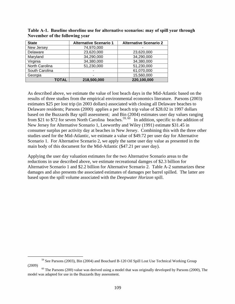
109

Table A-1. Baseline shoreline use for alternative scenarios: may of spill year through

November of the following year

State Alternative Scenario 1 Alternative Scenario 2

New Jersey 74,970,000 -

Delaware 23,620,000 23,620,000

Maryland 34,290,000 34,290,000

Virginia 34,380,000 34,380,000

North Carolina 51,230,000 51,230,000

South Carolina - 61,070,000

Georgia - 15,560,000

TOTAL 218,500,000 220,100,000

As described above, we estimate the value of lost beach days in the Mid-Atlantic based on the

results of three studies from the empirical environmental economics literature. Parsons (2003)

estimates $25 per lost trip (in 2003 dollars) associated with closing all Delaware beaches to

Delaware residents; Parsons (2000) applies a per beach trip value of $28.02 in 1997 dollars

based on the Buzzards Bay spill assessment; and Bin (2004) estimates user day values ranging

from $21 to $72 for seven North Carolina beaches.59, 60

In addition, specific to the addition of

New Jersey for Alternative Scenario 1, Leeworthy and Wiley (1991) estimate $31.45 in

consumer surplus per activity day at beaches in New Jersey. Combining this with the three other

studies used for the Mid-Atlantic, we estimate a value of $49.72 per user day for Alternative

Scenario 1. For Alternative Scenario 2, we apply the same user day value as presented in the

main body of this document for the Mid-Atlantic ($47.21 per user day).

Applying the user day valuation estimates for the two Alternative Scenario areas to the

reductions in use described above, we estimate recreational damges of $2.3 billion for

Alternative Scenario 1 and $2.2 billion for Alternative Scenario 2. Table A-2 summarizes these

damages and also presents the associated estimates of damages per barrel spilled. The latter are

based upon the spill volume associated with the Deepwater Horizon spill.

59 See Parsons (2003), Bin (2004) and Bouchard B-120 Oil Spill Lost Use Technical Working Group

(2009) 60 The Parsons (200) value was derived using a model that was originally developed by Parsons (2000), The

model was adapted for use in the Buzzards Bay assessment.

110

Table A-2. Shoreline use damages summary for alternative scenarios

Scenario Number of Lost Visits

Value Per Trip

($2017) Total

Damages

Per-Barrel Impact ($2017)

Alternative Scenario 1: Mid-Atlantic and New Jersey 45,360,000 $49.72 $2.3 billion $707

Alternative Scenario 2: Mid-Atlantic, South Carolina, and Georgia 45,700,000 $47.21 $2.2 billion $676

INLAND FISHING

To determine the baseline number of recreational inland fishing trips in New Jersey, South

Carolina, and Georgia, we rely on inland angler trip data from NOAA’s MRIP.61

Using the same

procedures as outlined in Chapter 3 of this document for the Mid-Atlantic states, we estimate the

baseline values shown in Table A-3. To estimate the reduction in inland fishing activity for each

of the Alternative Scenarios, we assume a 32.5 percent reduction in use for May of the spill year

through January of the following year and a 10 percent reduction in February and March of the

following year, consistent with reductions applied in the main body of this document for the

Mid-Atlantic. Applying these values to the baseline angler trips for each Alternative Scenario,

we estimate approximately 3.0 million lost angler trips under Alternative Scenario 1 and 2.7

million lost angler trips under Alternative Scenario 2.

Table A-3. inland fishing baseline for alternative scenarios: May of spill year through

March the following year

State Alternative Scenario 1 Alternative Scenario 2

New Jersey 2,570,000 -

Delaware 650,000 650,000

Maryland 2,410,000 2,410,000

Virginia 2,230,000 2,230,000

North Carolina 1,830,000 1,830,000

South Carolina - 980,000

Georgia - 620,000

TOTAL 9,690,000 8,730,000

To estimate the value of lost fishing trips, we rely upon per-trip estimates from the empirical

literature summarized in Chapter 3 plus additional estimates from McConnell and Strand (1994)

for New Jersey, South Carolina, and Georgia. Combining the New Jersey value ($74.78) with

the other estimates we identified for the Mid-Atlantic, we estimate a value of $77.38 per fishing

trip for Alternative Scenario 1. Similarly, integrating the South Carolina and Georgia values

($144.25 and $87.60, respectively) with the estimates for the Mid-Atlantic yields an estimate of

$90.23 per fishing trip for Alternative Scenario 2.

Based on the per trip fishing values for Alternative Scenarios 1 and 2 and the estimated

reductions in inland fishing for each scenario, we estimate inland fishing losses of $234.7 million

61 See NOAA (2014)

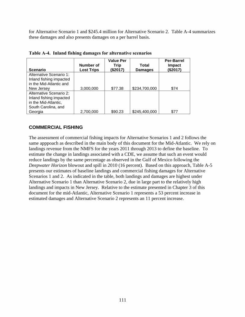
111

for Alternative Scenario 1 and $245.4 million for Alternative Scenario 2. Table A-4 summarizes

these damages and also presents damages on a per barrel basis.

Table A-4. Inland fishing damages for alternative scenarios

Scenario Number of Lost Trips

Value Per Trip

($2017) Total

Damages

Per-Barrel Impact ($2017)

Alternative Scenario 1: Inland fishing impacted in the Mid-Atlantic and New Jersey 3,000,000 $77.38 $234,700,000 $74

Alternative Scenario 2: Inland fishing impacted in the Mid-Atlantic, South Carolina, and Georgia 2,700,000 $90.23 $245,400,000 $77

COMMERCIAL FISHING

The assessment of commercial fishing impacts for Alternative Scenarios 1 and 2 follows the

same apppoach as described in the main body of this document for the Mid-Atlantic. We rely on

landings revenue from the NMFS for the years 2011 through 2013 to define the baseline. To

estimate the change in landings associated with a CDE, we assume that such an event would

reduce landings by the same percentage as observed in the Gulf of Mexico following the

Deepwater Horizon blowout and spill in 2010 (16 percent). Based on this approach, Table A-5

presents our estimates of baseline landings and commercial fishing damages for Alternative

Scenarios 1 and 2. As indicated in the table, both landings and damages are highest under

Alternative Scenario 1 than Alternative Scenario 2, due in large part to the relatively high

landings and impacts in New Jersey. Relative to the estimate presented in Chapter 3 of this

document for the mid-Atlantic, Alternative Scenario 1 represents a 53 percent increase in

estimated damages and Alternative Scenario 2 represents an 11 percent increase.

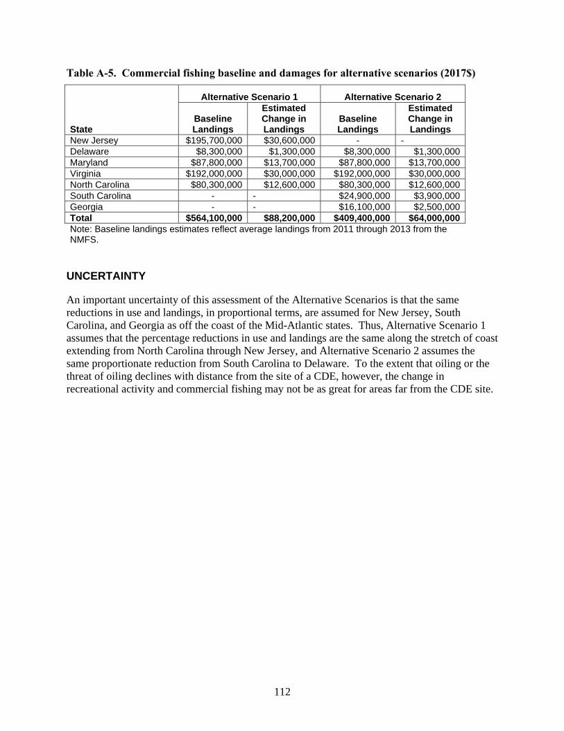
112

Table A-5. Commercial fishing baseline and damages for alternative scenarios (2017$)

State

Alternative Scenario 1 Alternative Scenario 2

Baseline Landings

Estimated Change in Landings

Baseline Landings

Estimated Change in Landings

New Jersey $195,700,000 $30,600,000 - -

Delaware $8,300,000 $1,300,000 $8,300,000 $1,300,000

Maryland $87,800,000 $13,700,000 $87,800,000 $13,700,000

Virginia $192,000,000 $30,000,000 $192,000,000 $30,000,000

North Carolina $80,300,000 $12,600,000 $80,300,000 $12,600,000

South Carolina - - $24,900,000 $3,900,000

Georgia - - $16,100,000 $2,500,000

Total $564,100,000 $88,200,000 $409,400,000 $64,000,000

Note: Baseline landings estimates reflect average landings from 2011 through 2013 from the NMFS.

UNCERTAINTY

An important uncertainty of this assessment of the Alternative Scenarios is that the same

reductions in use and landings, in proportional terms, are assumed for New Jersey, South

Carolina, and Georgia as off the coast of the Mid-Atlantic states. Thus, Alternative Scenario 1

assumes that the percentage reductions in use and landings are the same along the stretch of coast

extending from North Carolina through New Jersey, and Alternative Scenario 2 assumes the

same proportionate reduction from South Carolina to Delaware. To the extent that oiling or the

threat of oiling declines with distance from the site of a CDE, however, the change in

recreational activity and commercial fishing may not be as great for areas far from the CDE site.

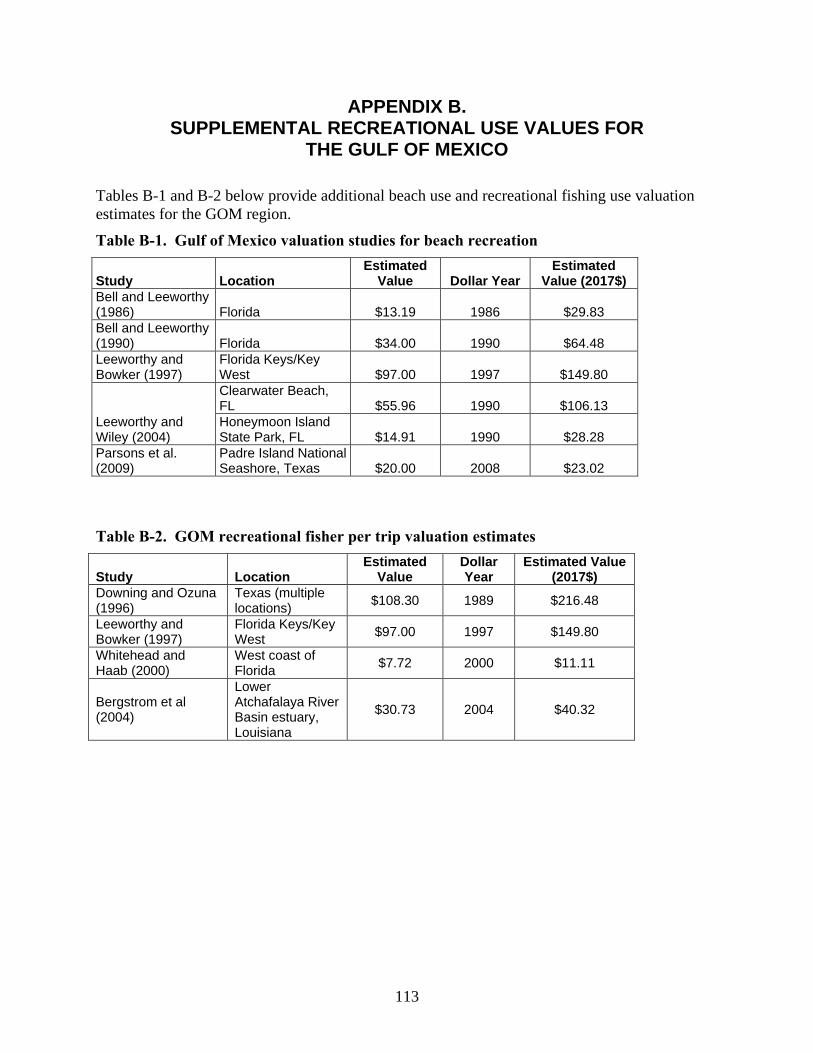
113

APPENDIX B. SUPPLEMENTAL RECREATIONAL USE VALUES FOR

THE GULF OF MEXICO

Tables B-1 and B-2 below provide additional beach use and recreational fishing use valuation

estimates for the GOM region.

Table B-1. Gulf of Mexico valuation studies for beach recreation

Study Location Estimated

Value Dollar Year Estimated

Value (2017$)

Bell and Leeworthy (1986) Florida $13.19 1986 $29.83

Bell and Leeworthy (1990) Florida $34.00 1990 $64.48

Leeworthy and Bowker (1997)

Florida Keys/Key West $97.00 1997 $149.80

Leeworthy and Wiley (2004)

Clearwater Beach, FL $55.96 1990 $106.13

Honeymoon Island State Park, FL $14.91 1990 $28.28

Parsons et al. (2009)

Padre Island National Seashore, Texas $20.00 2008 $23.02

Table B-2. GOM recreational fisher per trip valuation estimates

Study Location Estimated

Value Dollar Year

Estimated Value (2017$)

Downing and Ozuna (1996)

Texas (multiple locations)

$108.30 1989 $216.48

Leeworthy and Bowker (1997)

Florida Keys/Key West

$97.00 1997 $149.80

Whitehead and Haab (2000)

West coast of Florida

$7.72 2000 $11.11

Bergstrom et al (2004)

Lower Atchafalaya River Basin estuary, Louisiana

$30.73 2004 $40.32