Forecasting Methods and Principles: Evidence-Based Checklists

J. Scott Armstrong1 and Kesten C. Green2

ABSTRACT Problem: How to help practitioners, academics, and decision makers use experimental research findings to

substantially reduce forecast errors for all types of forecasting problems. Methods: Findings from our review of forecasting experiments were used to identify methods and principles

that lead to accurate forecasts. Cited authors were contacted to verify that summaries of their research were correct. Checklists to help forecasters and their clients practice and commission studies that adhere to principles and use valid methods were developed. Leading researchers were asked to identify errors of omission or commission in the analyses and summaries of research findings.

Findings: Forecast accuracy can be improved by using one of 15 relatively simple evidence-based forecasting methods. One of those methods, knowledge models, provides substantial improvements in accuracy when causal knowledge is good. On the other hand, data models—developed using multiple regression, data mining, neural nets, and “big data analytics”—are unsuited for forecasting.

Originality: Three new checklists for choosing validated methods, developing knowledge models, and assessing uncertainty are presented. A fourth checklist, based on the Golden Rule of Forecasting, was improved.

Usefulness: Combining forecasts within individual methods and across different methods can reduce forecast errors by as much as 50%. Forecasts errors from currently used methods can be reduced by increasing their compliance with the principles of conservatism (Golden Rule of Forecasting) and simplicity (Occam’s Razor). Clients and other interested parties can use the checklists to determine whether forecasts were derived using evidence-based procedures and can, therefore, be trusted for making decisions. Scientists can use the checklists to devise tests of the predictive validity of their findings.

Key words: combining forecasts, data models, decomposition, equalizing, expectations, extrapolation, knowledge models, intentions, Occam’s razor, prediction intervals, predictive validity, regression analysis, uncertainty

Authors’ notes:

1. This paper will be published in the Journal of Global Scholars of Marketing Science. We were pleased to do so because of the interest by their new editor, Arch Woodside, in papers with useful findings, and the journal’s promise of fast decisions and publication, offer of OpenAccess publication, and policy of publishing in both English and Mandarin. The journal has also supported our use of a structured abstract and provision of links to cited papers to the benefit of readers.

2. We received no funding for this paper and have no commercial interests in any method. 3. Most readers should be able to read this paper in less than one hour. 4. We endeavored to conform with the Criteria for Science Checklist at GuidelinesforScience.com.

Acknowledgments: We thank our reviewers, Hal Arkes, Kay A. Armstrong, Roy Batchelor, David Corkindale, Alfred G. Cuzán, John Dawes, Robert Fildes, Paul Goodwin, Andreas Graefe, Rob Hyndman, Randall Jones, Magne Jorgensen, Spyros Makridakis, Kostas Nikolopoulos, Keith Ord, Don Peters, and Malcolm Wright. Thanks also to those who made useful suggestions: Raymond Hubbard, Frank Schmidt, Phil Stern, and Firoozeh Zarkesh. And to our editors: Harrison Beard, Amy Dai, Simone Liao, Brian Moore, Maya Mudambi, Esther Park, Scheherbano Rafay, and Lynn Selhat. Finally, we thank the authors of the papers that we cited for their substantive findings for their prompt confirmation and useful suggestions on how to best summarize their work.

1 The Wharton School, University of Pennsylvania, Philadelphia, PA 19104, U.S.A. and Ehrenberg-Bass Institute, University of South Australia Business School: +1 610 622 6480; armstrong@wharton.upenn.edu 2 School of Commerce and Ehrenberg-Bass Institute, University of South Australia Business School, University of South Australia, City West Campus, North Terrace, Adelaide, SA 5000; kesten.green@unisa.edu.au.

2

INTRODUCTION

Forecasts are important for decision-making in businesses and other organizations, and for governments. A survey of practitioners, educators, and decision-makers found that they rated “accuracy” as the most important of 13 criteria for judging forecasts (Yokum and Armstrong, 1995). Researchers were especially concerned with accuracy. Consistent with that finding, improving forecast accuracy is the primary concern of this paper.

Since the 1930s, researchers have responded to the need for accurate forecasts by conducting experiments testing multiple reasonable methods. The findings from those ground-breaking experiments have greatly improved forecasting knowledge. In the late-1990s, 39 forecasting researchers from a variety of disciplines summarized scientific knowledge on forecasting. They were assisted by 123 expert reviewers (Armstrong 2001). The findings were used to develop 139 principles (condition-action statements), for forecasting in various situations. In 2015, two papers further condensed forecasting knowledge as two overarching principles: simplicity and conservatism (Green and Armstrong 2015, and Armstrong, Green, and Graefe 2015, respectively).

While the advances in forecasting knowledge allow for substantial improvements in forecast accuracy, that knowledge is largely ignored in academic journal articles and, we expect, also by practitioners. At the time that the original 139 forecasting principles were published in 2001, a review of 17 forecasting textbooks found that the typical book mentioned only 19% of the principles (Cox and Loomis 2001). Moreover, forecasting software packages, which could help to ensure that the principles are used, were found to ignore about half of the forecasting principles (Tashman and Hoover 2001).

CHECKLISTS TO IMPROVE FORECASTING

The use of evidence-based checklists avoids the need for memorizing and simplifies complex tasks. In

fields such as medicine, aeronautics, and engineering, a failure to follow an appropriate checklist can be grounds for a lawsuit.

The use of checklists is supported by much research (e.g., Hales and Pronovost 2006). One experiment assessed the effects of using a 19-item checklist for a hospital procedure. The study compared thousands of patient outcomes in hospitals in eight cities around the world before and after the checklist was used. Use of the checklist reduced deaths from 1.5% to 0.8% in the month after the medical procedures (Haynes et al. 2009). Importantly, checklists improve decision-making even when the knowledge incorporated in them is well-known to practitioners, and is known to be important (Hales and Pronovost 2006). To ensure that they include the latest evidence, checklists should be revised routinely.

Convincing people to use checklists is easy. When engineers and medical doctors are told they must use the checklist as a condition of their employment, and when use of the checklist is monitored, they use the checklists. When we have paid people modest sums to complete tasks by using checklists, almost all of those who accepted the task did so effectively. For example, to assess the persuasiveness of print advertisements, raters hired through Amazon’s Mechanical Turk used a 195-item checklist to evaluate advertisements’ conformance to persuasion principles. The inter-rater reliability was high (Armstrong, Du, Green, and Graefe 2016).

3

RESEARCH METHODS

We reviewed prior experimental research on which forecasting methods and principles lead to improved forecast accuracy. To do so, we first identified relevant research by:

1) searching the Internet, mostly using Google Scholar; 2) contacting leading researchers for suggestions of important experimental findings; 3) checking key papers referred to in experimental studies and meta-analyses; 4) putting our working paper online with requests for evidence that we might have overlooked; 5) providing links to all papers in an OpenAccess version of this paper in order to allow readers to check

our interpretations of the original findings. Given the enormous number of papers with promising titles, we screened papers by assessing whether

the “Abstract” or “Conclusions” sections provided evidence on the comparative value of alternative methods, and full disclosure. Only a small percentage of the papers with promising titles met those criteria.

Only studies that examine many out-of-sample (ex ante) forecasts are considered as evidence in this paper. For cross-sectional data, the “jack-knife” procedure allows for many forecasts by using all but one data point to estimate the model, making a forecast for the excluded observation, then replacing that observation and excluding another, and so on until forecasts have been made for all data points. Successive updating can be used to increase the number of out-of-sample forecasts for time-series data. For example, to test the predictive validity of alternative models for forecasting the next 100 years of global mean temperatures, annual forecasts were made for horizons from one to 100 years-ahead starting in 1851. The forecasts were updated as if in 1852, then 1853, and so on, thus providing errors for 157 one-year-ahead forecasts… and 58 one-hundred-year-ahead forecasts (Green, Armstrong, and Soon 2009).

We attempted to contact the authors of all papers that we cited regarding substantive findings. We did so on the basis of evidence that findings cited in papers in leading scientific journals are often described incorrectly (Wright and Armstrong 2008). We asked the authors if our summary of their findings was correct and whether our description could be improved. We also asked them to suggest relevant papers that we had overlooked—especially papers describing experiments with findings that conflicted with our conclusions. That practice was shown to contribute to a substantially more comprehensive search for evidence than was achieved by computer searches (Armstrong and Pagell 2003). In the case of six papers, we could not agree with the authors on the interpretation of findings. We discarded our citations of those papers, as they were not essential to the purpose of this paper.

Of the 90 papers with substantive findings that were not our own, we were able to contact the authors of 73 and received substantive, and often helpful, replies from 69. We coded the papers in the references section of this paper, including the results of our efforts to contact authors.

Our review led to the development of five checklists. They provide evidence-based guidance on forecasting methods, knowledge models, the Golden Rule of Forecasting, simplicity, and uncertainty.

VALID FORECASTING METHODS: CHECKLIST AND EVIDENCE

The predictive validity of a forecasting method is assessed by comparing the accuracy of forecasts from

the method with the accuracy of forecasts from currently used methods, or from simple benchmark methods such as the naïve no-trend model, or from other evidence-based methods. Such testing of multiple reasonable hypotheses is a requirement of the scientific method as described by Chamberlin (1890).

For categorical forecasts—such as whether a, b, or c will happen, or which of them would be better—accuracy is typically measured as a variation of percent correct. For quantitative forecasts, accuracy is assessed by differences between ex ante forecasts and data on what actually transpired. The benchmark error measure for evaluating forecasting methods is the Relative Absolute Error, or “RAE.” It has been shown to be more reliable than the Root Mean Square Error (Armstrong and Collopy 1992). Tests of a new method—a development of the RAE—called the Unscaled Mean Bounded Relative Absolute Error (UMBRAE)—suggest that it is superior to the RAE and other proposed alternatives (Chen, Twycross, and Garibaldi 2017). We suggest using both the RAE

4

and UMBRAE until additional testing has been done to provide a definitive conclusion on which is the better measure.

Exhibit 1 lists 15 individual evidence-based forecasting methods. They are consistent with forecasting principles and have been shown to provide out-of-sample forecasts with superior accuracy. The Exhibit also identifies the knowledge needed to use each method. Combining within and across methods is recommended (Checklist items 16 and 17.)

Exhibit 1: Forecasting Methods Application Checklist

Name of forecasting problem: ________________________________________________________________

Forecaster: ____________________________________________________ Date: ______________________

Method Knowledge needed Usable method

Variations within

components Forecaster* Respondents/Experts† () (Number)

Judgmental methods 1. Prediction markets Survey/market design Domain; Problem [ ] 2. Multiplicative decomposition Domain; Structural relationships Domain [ ] 3. Intentions surveys Survey design Own plans/behavior [ ] 4. Expectations surveys Survey design Others’ behavior [ ] 5. Expert surveys (Delphi, etc.) Survey design Domain [ ] 6. Simulated interaction Survey/experimental design Normal human responses [ ] 7. Structured analogies Survey design Analogous events [ ] 8. Experimentation Experimental design Normal human responses [ ] 9. Expert systems Survey design Domain [ ]

Quantitative methods (Judgmental inputs sometimes required) 10. Extrapolation Time-series methods; Data n/a [ ] 11. Rule-based forecasting Causality; Time-series methods Domain [ ] 12. Judgmental bootstrapping Survey/Experimental design Domain [ ] 13. Segmentation Causality; Data Domain [ ] 14. Simple regression Causality; Data Domain [ ] 15. Knowledge models Cumulative causal knowledge Domain [ ] 16. Combining forecasts from a single method… SUM of VARIATIONS [ ] 17. Combining forecasts from several methods… COUNT of METHODS [ ]

*Forecasters must always know about the forecasting problem, which may require consulting with the forecast client and domain experts, and consulting the research literature. †Experts who are consulted by the forecaster about their domain knowledge should be aware of relevant findings from experiments. Failing that, the forecaster is responsible for obtaining that knowledge.

For most forecasting problems, several of the methods will be usable, and should be used, as we describe

below. An electronic version of the Exhibit 1 checklist is provided at ForecastingPrinciples.com in the top menu bar under “Methods Checklist.”

Because we are concerned with methods that have been shown to improve forecast accuracy relative to methods that are commonly used in practice, we do not discuss all methods that have been used for forecasting. For example, multiple regression analysis is apparently one of the most widely used methods for developing forecasting models. Given the evidence summarized in this paper, however, we recommend against the use of multiple regression analysis and other data modeling approaches.

5

Clients should ask forecasters what methods they will use and why. If they mention a method that is not listed in Exhibit 1, they should be asked to produce evidence that their method provides forecasts with smaller errors than the relevant methods listed in the Exhibit.

Judgmental Methods

Expertise based on experience in similar situations can be useful for forecasting. Experience can lead to

simple “rules of thumb,” or heuristics, that provide quick forecasts for rapid decision-making. For example, the emergency landing of US Airways Flight 1549—the “Miracle on the Hudson”—was a success because the pilot used the gaze heuristic to forecast that landing on the Hudson River was a viable option, whereas returning to La Guardia Airport was not (Hafenbradl, Waeger, Marewski, and Gigerenzer 2016). Extensive research conducted by Gerd Gigerenzer and the ABC group of the Max Planck Institute for Human Development in Berlin has found that simple heuristics are superior to more complex and information intensive methods for many practical problems.

For situations in which there are two or more important causal factors and where experts do not receive frequent well-summarized feedback on the accuracy of their predictions, however, expertise and experience are, on their own, of no apparent value. Such situations are common in business and government decision making. Even leading experts’ unaided judgmental forecasts often turn out to be disastrously wrong, sometimes to the delight of the media (e.g., see Cerf and Navasky 1998; Perry 2017).

Research on the accuracy of experts’ unaided judgmental forecasts about complex situations dates from the early 1900s. An early review of the research led to the Seer-Sucker Theory: “No matter how much evidence exists that seers do not exist, suckers will pay for the existence of seers” (Armstrong 1980). The Seer-Sucker Theory has held up well over the years; in particular, a 20-year study comparing the accuracy of many forecasts from experts with those of forecasts from novices and from naïve rules provided support (Tetlock 2005).

While unaided expert judgments should be avoided, topic experts can play a vital role in forecasting when their judgments are incorporated using evidence-based methods. The next section describes nine structured methods for forecasting using expert judgment. 1. Prediction markets

Prediction markets—also known as betting markets, information markets, and futures markets—have been used for forecasting since the 16th century (Rhode and Strumpf 2004). Monetary rewards attract people who believe they have knowledge or information that enables them to make accurate predictions about the situation they are betting on.

Prediction markets are especially useful when knowledge is dispersed and many participants are motivated to trade repeatedly. Markets can rapidly revise forecasts when new information becomes available. Forecasters using prediction markets need to be familiar with designing prediction markets and surveys.

The accuracy of forecasts from prediction markets was tested in eight published comparisons in the field of business forecasting (Graefe 2011). The results were mixed. For example, prediction markets’ out-of-sample forecast errors were 28% smaller than those from no-change models in one comparison. On the other hand, averaging people’s judgments outperformed market forecasts in two of three comparisons. In another comparison, forecasts from the Iowa Electronic Market (IEM) prediction market across the 100 days before each U.S. presidential election from 2004 though 2016 were, on average, less accurate than forecasts from the RealClearPolitics poll average, a survey of experts, and citizen forecasts (Graefe 2017a). The IEM prediction market limits the bets to no more than $500, which likely reduces the number and motivation of participants. Comparative accuracy tests based on 44 elections in eight countries other than the U.S., however, found that forecasts from betting markets were more accurate than forecasts by experts, econometric models, and polls (Graefe 2017b).

6

2. Multiplicative decomposition

Decomposition has long been a key element of forecasting. A Google search for “decomposition” and either “forecast” or “predict” found over 45 million results in December 2017.

Multiplicative decomposition involves dividing a forecasting problem into parts, forecasting each part separately, and multiplying the forecasts of the parts to forecast the whole. For example, to forecast sales for a brand, a firm might separately forecast total market sales and market share, and then multiply those components. Decomposition is expected to be most effective at reducing forecast errors when suitable forecasting methods, data availability, and directional effects of causal factors vary among the parts.

To assess the effect of decomposition on forecast accuracy, subjects in an experiment were presented with five problems from an almanac, such as “How many packs (rolls) of Polaroid color films do you think were used in the United States in 1970?” Some subjects were asked to make estimates of the total figure, while others were asked to estimate each of the decomposed elements (Armstrong, Denniston, and Gordon 1975). Across that study and two similar studies, forecast error was reduced by an average of 42% (MacGregor 2001).

Another study used graphical software to display the 68 monthly series from the M-Competition (Makridakis et al. 1982) in ways that were designed to help users identify and forecast seasonality and trend independently using their judgment. The study found that three postgraduate students with knowledge of time series analysis and the software produced forecasts for one to 12 months into the future that had errors that were 7% less than those from the leading M-Competition method of deseasonalized single exponential smoothing. The error reduction from software-assisted judgmental decomposition by 35 novices forecasting five time-series each was 5% (Table II, Edmundson 1990).

3. Intentions surveys

Intentions surveys ask people how they plan to behave in specified situations. They can be used, for example, to predict how people would respond to major changes in the design of a product. One meta-analysis included 47 comparisons with over 10,000 subjects, and another provided a meta-analysis of 10 meta-analyses involving over 83,000 subjects. Both found a strong relationship between people’s intentions and their future behavior (Kim and Hunter 1993; Sheeran 2002).

Intentions surveys are especially useful when historical data are not available. They are most likely to provide useful forecasts for short forecast time-horizons, and for important decisions (Morwitz 2001; Morwitz, Steckel, and Gupta 2007).

To assess people’s intentions, the forecaster should prepare brief unbiased descriptions of the situation (Armstrong and Overton 1971). Intentions should be expressed as probabilities such as 0 = ‘No chance, or almost no chance (1 in 100)’, to 10 = ‘Certain, or practically certain (99 in 100).’ Responses can be used to calculate a forecast of how people will behave, such as “3.2% of the population will buy the product in the next three months” (Morwitz 2001).

The way a question is asked can have a large effect on responses. Two ways to reduce response error are to: (1) pretest the questions to ensure that the respondents understand them in the way the forecaster intends, and (2) use alternative ways to state a question, then average responses across questions. For more advice, see Bradburn, Sudman, and Wansink (2004).

Including a monetary incentive to respond along with the questionnaire reduces non-response error (Armstrong and Yokum 1994). The forecasters should resend the questionnaire to non-responders in follow-up waves. Doing so allows one to estimate the effect of non-response by extrapolating across waves (Armstrong and Overton 1977). Additional evidence-based procedures for selecting samples and obtaining high response rates are described in Dillman, Smyth, and Christian (2014).

4. Expectations surveys

Expectations surveys ask people how they expect they or others will behave. Expectations differ from intentions because people realize that the situation can change. For example, if you were asked whether you intend to purchase a vehicle over the next year, you might say that you have no intention of doing so. However, you realize that it is possible that your vehicle will develop a major problem. As a consequence, you might expect

7

that there is a chance that you will purchase a new car. As with intentions surveys, expectations surveys should use probability scales, follow evidence-based procedures for survey design, use representative samples, obtain high response rates, and correct for non-response bias by extrapolating across waves.

Following the U.S. government’s 1932 prohibition of prediction markets for political elections, expectation surveys—which poll a representative sample of potential voters on how others would vote—were introduced (Hayes 1936). Those “citizen expectations” surveys correctly predicted the popular vote winners of the U.S. Presidential elections in 89% of the 217 surveys from 1932 to 2012. Furthermore, citizens’ expectations provided more accurate out-of-sample forecasts of the national vote share than polls, prediction markets, models, and experts across the seven U.S. Presidential elections from 1988 to 2012 (Graefe 2014), and again in 2016. Over the 100 days before the 2016 election, the error of citizens’ expectations forecasts of the popular vote in seven U.S. Presidential elections from 1992 through 2016 averaged 1.2 percentage points. In comparison, the error of a typical poll aggregator was, at 2.6 percentage points, more than twice as high. (Graefe, Armstrong, Jones, and Cuzan, 2017). 5. Expert surveys

Use written questions and instructions for self-completion surveys to ensure that each expert is questioned in the same way. Apply the same procedures for developing questions as those described for expectations surveys above.

Forecasters should obtain forecasts from at least five experts, and up to 20 for important forecasts (Hogarth 1978). That advice was followed in forecasting the popular vote for U.S. Presidential elections from 2004 to 2016, when surveys of about fifteen experts led to an average error of 1.6 percentage points, compared to 1.7 percentage points for combined polls (Graefe, Armstrong, Jones, and Cuzan 2017, and personal correspondence with Graefe). Additional advice on the design of expert surveys is provided in Armstrong (1985, pp.108-116).

Delphi is an extension of the expert survey approach whereby the survey is conducted over two or more rounds. After each round, anonymous summaries of the experts’ forecasts and reasons are provided to the experts. The process is repeated until forecasts change little between rounds—usually two or three rounds are sufficient. Use the median or mode of the experts’ final-round forecasts as the Delphi forecast. Delphi is expected to be most useful when the different experts each have different information relevant to the problem (Jones, Armstrong, and Cuzan 2007).

Forecasts from Delphi were more accurate than forecasts from traditional meetings in five studies, about the same accuracy in two, and less accurate in one. Delphi forecasts were more accurate than forecasts from traditional surveys of expert opinion for 12 of 16 studies, with two ties and two cases in which Delphi was less accurate. Among those 24 comparisons, Delphi improved accuracy in 71% and harmed it in 12% (Rowe and Wright 2001).

Delphi is attractive to managers because judgments from dispersed experts can be obtained without the expense of arranging meetings. It has an advantage over prediction markets in that the participants provide reasons for their forecasts (Green, Armstrong, and Graefe 2007). Software for the procedure is freely available at ForecastingPrinciples.com.

6. Simulated interaction

Simulated interaction uses role-playing to forecast decisions by two or more parties with conflicting interests. Situations that have been used for testing the method include an attempt to secure an exclusive distribution arrangement with a major supplier, a union-management dispute over pay and conditions, and artists demanding that the government provide them with financial support.

The forecaster provides each role-player with a description of one the main protagonists’ roles, and a brief description of the situation including a list of possible decisions. The role-players are asked to engage in realistic interactions with one another, staying in their roles until a decision is reached. The simulations typically last less than an hour.

Relative to unaided expert judgment—the most common method—simulated interaction reduced forecast errors by 57% on average for eight conflict situations, including those described above and an attempted

8

hostile takeover of a corporation, and a military standoff between two countries over access to water (Green 2005). The method seems to work best when naïve role players do not know each other, have no prior opinions about the situation, and no agenda beyond that indicated by their role.

The alternative approach of “putting oneself in the other person’s shoes” has been proposed. U.S. Secretary of Defense Robert McNamara suggested that if he had done this during the Vietnam War, he would have made better decisions.3 A test of the “role-thinking” approach, however, found no improvement in forecast accuracy relative to that of unaided judgment. It is too difficult to think through the interactions in a complex situation—active role-playing between parties is necessary to provide sufficient realism (Green and Armstrong 2011).

7. Structured analogies

The structured analogies method involves asking ten or so experts to suggest situations that were similar to the one for which a forecast is required, the target situation. The experts are given a description of the target situation and are asked to identify analogous situations, rate their similarity to the target, and match the outcomes of their analogies with possible outcomes of the target situation. An administrator takes the target situation outcome implied by each expert’s top-rated analogy and calculates the modal outcome as the forecast. The method should not be confused with the common use of analogies to justify a decision that is preferred by the forecaster or client.

Structured analogies forecasts were 41% more accurate than unaided judgment forecasts in forecasting decisions in the eight real conflicts used in research on the simulated interaction method described above (Green and Armstrong 2007a). Structured analogies were also used to forecast the effects of incentives to promote laptop purchases by university students, and a program offering certification on Internet safety to parents of high school students. The error of those structured analogies forecasts was 8% lower than the error of forecasts from unaided judgment (Nikolopoulos, Petropoulos, Bougioukos, and Khammash 2015). A procedure akin to structured analogies was used to forecast box office revenue for 19 unreleased movies, in which raters identified analogous movies from a database and rated them for similarity. The revenue forecasts from the analogies were adjusted for advertising expenditure and whether the movie was a sequel. Errors from the structured analogies forecasts were less than half those of forecasts from simple and complex regression models (Lovallo, Clarke and Camerer 2012). Across the ten comparative tests from the three studies described above, the error reductions from using structured analogies averaged about 40%.

8. Experimentation

Experimentation is widely used and is the most valid and reliable method for determining cause-and-effect relationships. Knowledge of the direction of effects and estimates of the strength of effects can then be used to make forecasts. Experiments can be conducted in laboratories. An analysis of organizational behavior experiments found that laboratory experiments yielded similar findings to field experiments (Locke 1986).

Alternatively, forecasters can analyze natural experiments to identify causal relationships and make forecasts. For example, the regulation and deregulation of industries provided natural experiments on the effect of regulation on consumer welfare. Winston (1993) found that regulation harmed customers in eight of the nine markets for which such experimental data were available, and was of no net benefit in the case of the ninth market.

9. Expert systems

Expert systems are developed by asking experts to describe the steps they take while they make forecasts, then describing that process using software. The resulting expert system should be complete, simple, and clearly described.

A review of 15 comparisons found that expert system forecasts were more accurate than forecasts from unaided judgments (Collopy, Adya and Armstrong 2001). Two of the studies—on gas, and on mail order catalogue sales—found that the expert systems’ forecast errors were 10% and 5% smaller, respectively, than 3 From the 2003 documentary film, “Fog of War.”

9

those of unaided judgment. While the evidence available on predictive validity is scant, the method appears promising.

Quantitative Methods

Quantitative methods require numerical data on or related to the forecasting problem. Quantitative methods can also draw upon judgmental methods, such as decomposition, in order to make the best use of knowledge and data. These models also enable the explicit use of causal relationships.

This section describes six evidence-based quantitative forecasting methods. Other than the first of the methods (extrapolation), the methods rely heavily on causal knowledge to forecast the effects of changes in causal variables. Such forecasts can be used for policy making, and for developing contingency plans. Forecasting what will happen when the causal variables are out of the decision makers’ control, however, requires that the causal variables are accurately forecast. 10. Extrapolation

While extrapolation methods can be used for any problem requiring forecasts of a time series, they are especially useful when little is known about the factors affecting the forecast variable, causal variables are not expected to change much, or causal variables cannot be forecast with much accuracy.

Exponential smoothing, which dates back to Brown (1959 and 1962), is easy to understand. It is a sensible approach, because it uses all historical data in a moving average that puts more weight on the most recent data. For a review of exponential smoothing, see Gardner (2006).

One should not assume that a trend will continue at the same rate, even in the short-term. It could increase or decrease in response to changes in the causal forces that drive the trend. The greater the uncertainty about the situation, the greater is the need to damp the trend toward zero—the no change forecast. A review of 10 experimental comparisons found that, on average, damping the trend toward zero reduced forecast errors by almost 5% and reduced the risk of large errors compared to forecasts that assumed a constant trend (Armstrong 2006). Gardner’s software for damped-trend extrapolation can be found at ForcastingPrinciples.com. When there is a long-term trend and the causal factors are expected to continue—such as with the real prices of resources (Simon 1996)—damping toward the long-term trend is appropriate.

When extrapolating for time periods less than a year, estimate the effects of seasonal influences and remove them from the data. Forecast the seasonally-adjusted series, then “seasonalize” the forecasts. In forecasts for 68 monthly economic series over 18-month horizons from the M-Competition, seasonal adjustment reduced forecast errors by 23% (Makridakis, Andersen, Carbone, et al. 1984, Table 14).

Forecasters should damp statistical estimates of seasonal influences. Such estimates are uncertain and standard seasonal adjustment procedures tend to “overfit” the data. Miller and Williams (2003, 2004) provide procedures for damping seasonal factors. When they damped the seasonal adjustments for the 1,428 monthly time-series from the M3-Competition, the accuracy of the forecasts improved for 59% to 65% of the time series, depending on the horizon. The broad findings were replicated by Boylan, Goodwin, Mohammadipour, and Syntetos (2015). Software for the Miller-Williams procedures and the M3-Competition data are freely available at .

Damping by averaging seasonal factors across analogous series also improves forecast accuracy. In one study, combining seasonal factors from related products, such as snow blowers and snow shovels, reduced the average forecast error by about 20% (Bunn and Vassilopoulos 1999). In another study, pooling monthly seasonal factors for crime rates for six city precincts reduced the error of exponential smoothing forecasts by about 7% compared to using seasonal factors that were estimated individually for each precinct (Gorr, Oligschlager, and Thompson 2003, Figure 4).

Multiplicative decomposition can be used to incorporate causal knowledge into extrapolation forecasts. For example, when forecasting time-series data, it often happens that the series is affected by causal forces—characterized as growth, decay, opposing, regressing, supporting, or unknown. In such a case, one can decompose the time series by causal forces that have different directional effects, extrapolate each component, and then recombine. Doing so is likely to improve accuracy under two conditions: (1) domain knowledge can be used to structure the problem so that causal forces differ for two or more of the component series, and (2) it is

10

possible to obtain relatively accurate forecasts for each component. For example, to forecast motor vehicle deaths, one study forecast the number of miles driven, a series that would be expected to grow, and the death rate per million passenger miles, a series that would be expected to decrease due to better roads and safer cars. The two extrapolation forecasts were then multiplied to get total deaths. When tested on five time series that clearly met the two conditions, decomposition by causal forces reduced out-of-sample forecast errors by two-thirds. For the four series that partially met the conditions, decomposition by causal forces reduced error by one-half. There was no gain or loss in forecast accuracy when the conditions did not apply (Armstrong, Collopy, and Yokum 2005).

Additive decomposition can also be considered for extrapolation problems. One approach that is useful when the most recent data are uncertain or liable to subsequent revision is to forecast the starting level and trend separately, and then add them—a procedure called “nowcasting.” Three comparative studies found that, on average, nowcasting reduced errors for short-range forecasts by 37% (Tessier and Armstrong 2015). 11. Rule-based forecasting

Rule-based forecasting (RBF) uses knowledge about evidence-based extrapolation along with causal knowledge to forecast time-series data. To use RBF, first identify which of 28 “features” best characterize the series to be forecast. Features include forecast horizons, the amount of data available, and the existence of outliers. Then use the 99 RBF rules to weight the alternative extrapolation models and combine the models’ forecasts (Armstrong, Adya and Collopy 2001).

For one-year-ahead ex ante forecasts of 90 annual series from the M-Competition (available on ForecastingPrinciples.com), the Median Absolute Percentage Error of RBF forecasts was 13% smaller than that of equally weighted combined forecasts. For six-year-ahead ex ante forecasts, the RBF forecast errors were 42% smaller, likely due to the increasing importance of causal effects over longer horizons. RBF forecasts were also more accurate than equally weighted combinations of forecasts in situations involving strong trends, low uncertainty, stability, and good domain expertise. RBF forecasts had little or no accuracy advantage over unweighted combinations of forecasts for other situations (Collopy and Armstrong 1992). Testing by Vokurka, Flores, and Pearce (1996) provided supporting evidence for the relative accuracy of RBF forecasts.

One of the 99 RBF rules, the “contrary series rule” is especially important, as well as simple and inexpensive to apply. It states that one should not extrapolate a trend if the direction of a time series expected by domain experts is contrary to the recent trend of the time series. The use of that rule alone yielded improvements in extrapolating time-series data from five data sets. In particular, for longer-term (six-years ahead) forecasts, the error reductions exceeded 40% (Armstrong and Collopy 1993).

12. Judgmental bootstrapping

This method was developed in the early 1900s to provide forecasts of the size of the upcoming corn harvest in the U.S. In the 1940s, the method was used successfully for personnel selection (Meehl 1954) and has been supported by subsequent research (e.g., Dawes and Corrigan 1974; Grove, Zaid, Lebow, Snitz, and Nelson 2000). The method uses regression analysis to estimate coefficients for the variables that experts use to make judgmental forecasts. The dependent variable is not the outcome, but rather the experts’ predictions of the outcome given the values of the causal variables. Among researchers in forecasting, the method has, in recent decades, been called “judgmental bootstrapping.” In effect, it uses a quantitative model of the experts’ use of causal information for forecasting to improve upon the experts’ forecast accuracy.

In comparative studies to date, the bootstrap model’s forecasts were more accurate than those of the experts whose judgments they were based on. The gain in accuracy arises from the quantitative model’s more consistent application of the expert’s mental model. In addition, the model does not become distracted by irrelevant information and variables, nor does it become tired or irritable.

The first step for developing a judgmental bootstrap model is to ask experts to identify causal variables based on their domain knowledge. Then ask them to make predictions using data on the variables. For example, they could be asked to forecast the likelihood of success of doctoral candidates.

Judgmental bootstrap models can be estimated from experts’ predictions made on the basis of hypothetical data on the causal variables. Doing so allows the forecaster to ensure that the causal variables vary

11

substantially and independently of one another. That use of experimental design overcomes many of the deficiencies of multiple regression. It also enables one to make forecasts for situations for which actual data are not available. Once developed, the bootstrap model can provide forecasts at a low cost and for different situations—e.g., for a new product with different features.

Despite the discovery of the method and evidence on its usefulness, its early use was confined to agricultural predictions. Social scientists rediscovered the method in the 1960s, and tested its predictive validity. A review of those studies found that judgmental bootstrapping forecasts were more accurate than those from unaided judgments in eight of 11 comparisons, with two tests finding no difference and one finding a small loss in accuracy (Armstrong 2001a). The one failure occurred when the experts relied on an irrelevant variable that was not excluded from the bootstrap model. The typical error reduction was about 6% relative to unaided judgment.

Many universities taught the methods to their students, but we are aware of only one that adopted the method, despite the fact that one of the earliest validation tests showed that it provided a more accurate and less expensive way of predicting success in a PhD program (Dawes 1971).

In 2002, the Oakland Athletics baseball team adopted a version of judgmental bootstrapping. Attempts were made to block the use of the method by the experts who traditionally used their judgment to make the selection decisions—the managers, owners, and scouts. But the new general manager persisted, and the team performed well. Other professional sports teams subsequently adopted the method, improving both won-lost ratios and profitability (Armstrong 2012). 13. Segmentation

Segmentation in forecasting involves structuring the problem in order to make best use of knowledge and data about parts, or sub-populations, that are expected to behave differently. Appropriate methods are used to make forecasts for each part, and the forecasts for the parts are then added to derive a forecast for the whole. Segmentation attracted widespread attention when it was used to forecast the 1960 Kennedy-Nixon election outcome (Pool, Abelson and Popkin 1965).

The Port of New York Authority used the method in 1955 to forecast air travel demand ten years hence. Their analysts divided airline travelers into segments of 130 business traveler types and 160 personal traveler types. The personal travelers were segmented by age, then by occupation, income, and education; and the business travelers were segmented by occupation, then industry, and finally income. Data on each segment were obtained from the census and from a survey on travel behavior. To derive the forecast, the official projected air travel population for 1965 was allocated among the segments, and the number of travelers and trip frequency were extrapolated using 1935 as the starting year with zero travelers. The resulting forecast of 90 million trips was only 3% different from the actual 1965 figure (Armstrong 1985).

To use segmentation, identify important causal variables that can be used to define the segments, and their priorities. Then determine cut-points—e.g., different age categories of people—for each variable. Use more cut-points when there are non-linearities in the relationships and fewer cut points when the samples of data are smaller. Next, forecast the population of each segment and the behavior of the population within each segment by using the typical behavior. Finally, combine the population and behavior forecasts for each segment and sum across segments. The method is most likely to be useful when much data are available.

Segmentation is suitable for situations in which variables are interrelated, the effects of variables are non-linear, and prior causal knowledge is good. These conditions occurred, to a reasonable extent, in a study where data from 2,717 gas stations were used to estimate a segmentation model for forecasting weekly gasoline sales volumes. Data were available on nine binary variables and ten other variables including type of area, traffic volumes, length of street frontage, presence of a canopy, and whether the station was open 24 hours a day. The method was tested using a holdout sample of 3,000 stations. The segmentation model forecast errors (Mean Absolute Percentage Errors) were 29% smaller than the errors of a multiple regression model estimated using the same variables and data (Armstrong and Andress 1970).

A review of the literature on segmentation is provided by Armstrong (1985, Chapter 9). While the evidence on predictive validity is not substantial, the method is sensible, as it is based on decomposition. Interest

12

in segmentation fell away after the 1970s, but we expect that it would be more useful now than ever before, given the availability of large databases. 14. Simple regression

Simple regression analysis can be used to forecast the effect of changes in a single causal variable. The method is conservative in that it reduces the effect size estimate toward the mean—via the calculation of a constant term—in response to variations in the relationship found in the estimation data. For a forecasting model estimated using simple regression to be useful, one must be able to control or accurately forecast the causal variable.

The traditional form of a simple regression model is y = a + bx, where “y” is the variable to be forecast (dependent variable), “a” is the constant, “b” is the effect size, and “x” is the causal variable. The method is appropriate for forecasting problems that involve good prior knowledge about a strong causal relationship, along with valid and reliable data on the dependent and causal variables. A basic assumption is that the forecaster must be able to accurately control or forecast the causal variable.

Transform the data so that the simple regression model provides a realistic representation of the causal relationship. For example, calculating logarithms of the causal and dependent variables before estimating the model will result in an effect size estimate in the form of an elasticity. Elasticities are the percentage change in the variable to be forecast that would result from a one percent change in the causal variable. A price elasticity of demand of -1.2 for beef, for example, means that one would expect a price increase of 10% to result in a 12% decrease in the quantity demanded, all else being equal. Other transformations to consider include expressing the variables in per capita terms, and adjusting the data for the effect of currency inflation and seasonality.

The least squares method of estimating regression model coefficients has the effect of giving extreme data values an excessive influence on the estimate of the effect size. To avoid that, adjust or remove outliers from the estimation data. One way to do so—known as “winsorizing”—is to set the outlier to the value of the most extreme observation in which you have confidence (Tukey 1962). Forecasters should specify the rules for determining outliers before doing any analysis in order to avoid the temptation to make adjustments to support a preferred hypothesis. Another sensible approach is to estimate the regression model by minimizing the absolute error (e.g., Dielman 1986; Dielman 1989). Multiple regression

What if more than one causal variable is important? Multiple regression analysis (MRA) might seem to be an obvious solution, but its use with non-experimental data leads to multicollinearity and interactions among causal variables. In addition, data on the variables are typically subject to measurement errors and validity concerns that make assessing the relative weight of each variable problematic. That complexity puts MRA at a considerable disadvantage to simple regression as a method for estimating causal relationships: MRA fails Occam’s razor.

To our knowledge, MRA was adopted without any testing of its predictive validity. The first comparative test that we are aware of involved making ten-year ahead forecasts of the populations of 100 counties in North Carolina. A multiple regression model with six causal variables was used to make the forecasts. For comparison, six simple regressions were estimated, one for each variable; their forecasts were then averaged for each county. The Mean Absolute Percentage Error of forecasts from the MRA model was 64% higher than that of the combined simple-regression model forecasts (Namboodiri and Lalu 1971).

Another test obtained forecasts for 20 data sets using MRA models with from 3 to 19 causal variables. The data sets included problems such as predicting professors’ salaries and high school dropout rates. MRA was compared with an equal weights model using the same variables, and also with the simple “take-the-best” (causal variable) approach based on the forecaster’s information. The MRA produced 1% fewer correct forecasts than were obtained from equal weights models and 3% fewer than from the take-the-best approach (Table 5-4, Czerlinski, Gigerenzer and Goldstein, 1999).

MRA forecasts of the popular vote for U.S. Presidential elections from MRA models were available from eight leading political forecasters. Their accuracy was compared with those from a simple regression using the “best” variable (typically the “economy”). Forecasts were made for each of the last 100 days of the ten U.S.

13

Presidential election years from 1972 to 2008 (a total of 1,000 forecasts). The MRA forecasts were less accurate than the simple regression model forecasts with a Mean Absolute Error of 3.8% compared to 3.6% (Graefe and Armstrong 2012).

Data models

Beginning in the 1960s, advances in technology made it feasible for analysts to use tests of statistical significance to select multiple “predictor variables” and estimate relationships. We refer to the resulting models as “data models.” The trend started in the mid-1900s with stepwise regression. It spawned procedures with names such as big data, analytics, data mining, and neural nets. One claim is that objectivity is increased by letting the data speak for themselves. As we show below, in practice these techniques have the opposite effect.

Einhorn (p. 367, 1972) was among the first to warn against data models. He concluded, “Access to powerful new computers has encouraged routine use of highly complex analytic techniques, often in the absence of any theory, hypotheses, or model to guide the researcher's expectations of results.” He likened the practice to alchemy. For a further discussion of the deficiencies of regression analysis in practice, see Armstrong (2012b).

The only scientific way to identify relationships in complex situation is to conduct experiments to identify the effects of proposed causal variables under different conditions. Data models ignore cumulative scientific knowledge, and rely only on the data.

Despite the widespread understanding that correlation does not imply causation, data models are based on statistically significant correlations: not on causal relationships but on “predictor variables.”. About 32% of the 182 regression papers published in the American Economic Review in the 1980s relied on statistical significance for choosing predictor variables (Ziliak and McCloskey 2004). The situation was worse in the 1990s, as 74% of 137 such papers did so.

Statistical significance testing is detrimental to advances in science (Armstrong 2007a,b). A theoretical analysis titled “Why most published research findings are false” demonstrated how using statistical significance testing along with testing for a preferred hypothesis leads to the publication of incorrect research findings (Ioannidis 2005). Data models can be, and are, used to support any desired conclusions through such dubious practices as proposing hypotheses after analyzing the data, trying out variables in order to find ones that support a preferred hypothesis, discarding observations that do not support the desired hypothesis, selecting unreasonable null hypotheses, using large sample sizes to ensure statistical significance, and ignoring findings by other researchers that do not support the desired hypothesis. These procedures are common tactics in advocacy research. Armstrong and Green (2018) summarize evidence on the extent to which such questionable procedures are used in scientific journals.

Our searches have been unable to find any experimental comparisons showing that MRA or other data modeling techniques have out-of-sample predictive validity equal to that of the simple evidence-based methods identified in Exhibit 1. To the contrary, the evidence that we have found shows that data models are unsuited to forecasting.

A comprehensive analysis of the accuracy of data mining found that forecasts from data-mining models had consistently lower out-of-sample predictive validity than simple alternative models. In one test, the authors of the study asked a data-mining expert to make predictions using a set of data. The expert did so, and identified many statistically significant relationships in the data. Unbeknownst to the data miner, the numbers were random (Keogh and Kasetty 2003) In personal correspondence with us, Keogh stated, “although I read every paper on time-series data mining, I have never seen a paper that convinced me that they were doing anything better than random guessing for prediction. Maybe there is such a paper out there, but I doubt it.”

15. Knowledge models

Some forecasting problems are characterized by knowledge of many important causal variables. Consider, for example, predicting which players will do well in sports, who would be an effective company executive, which countries will have the highest economic growth, or which applicants for immigration are most likely to pose a security risk. Knowledge models are suitable for such problems.

Benjamin Franklin proposed a form of a knowledge model in a letter to his friend, Joseph Priestley, who had written to Franklin about a “vexing decision” he was struggling to make. Franklin’s method was to list pros

14

and cons for each alternative giving each a subjective weight, then to sum the lists to determine which alternative has the largest score in its favor. Franklin called his approach “prudential algebra.” 4

A similar approach, called “experience tables,” was used in the early 1900s for deciding which prisoners should be given parole (Burgess 1936). Another version was called “configural analysis.” It came into limited use in the mid-1900s. The approach was found to have predictive validity (e.g., see Babst, Gottfredson and Ballard, 1968). Yet another version was developed more recently under the term “index method” where there was considerable testing as we describe below.

We propose the name “knowledge model” because the term is more descriptive than the previous terms. Exhibit 2 provides a checklist for developing a knowledge model.

Exhibit 2: Knowledge Model Development Checklist

a. Identify all important causal variables using domain knowledge and findings from experiments b. Discard a causal variable if it cannot be controlled, or accurately forecast c. Determine the directions of causal variables’ effects on the variable to be forecast d. Determine the relative magnitudes of causal variables’ effects on the variable to be forecast if possible e. Specify model as dependent variable score equals the sum of weighted causal variables f. Estimate relationship between scores and dependent variable values by regression analysis if feasible

a. Identify all important causal variables using domain knowledge and findings from experiments—

Follow the scientific method by using prior knowledge to identify causal variables. With knowledge models, causal variables can be as simple as binary; for example, “is taller than opponent” for an election forecasting model. In some situations, causal variables are obvious from logical relationships. In cases where they are not, consider surveying three to five domain experts. When the validity of a proposed causal variable is uncertain, consult findings from experiments, especially meta-analyses of experiments, in order to determine whether there is sufficient support for the use of the variable. Consider this example as an illustration of the importance of relying on experimental evidence: evidence on the direction of the effect of each of 56 persuasion principles from Armstrong (2010) was obtained from non-experimental data as well as from experimental data. The findings from different experiments were in the same direction for each principle, but for only two-thirds of the principles in the non-experimental data (Armstrong and Patnik 2009).

b. Discard a causal variable if it cannot be controlled, or accurately forecast—If a causal variable cannot be forecast or controlled, including it in a model can only harm the accuracy of forecasts from the model.

c. Determine the directions of causal variables’ effects on the variable to be forecast—The directional effects of some variables are obvious from logic or common knowledge about the domain. If the direction is not obvious, refer to experimental studies. For example, opinions about the effects of gun regulations on crime vary and opposing opinions among voters and politicians have led U.S. counties and states to change their laws to either restrict or make gun ownership easier. These natural experiments provide a method to scientifically determine which opinion is correct, as was done by Lott (2010) and Lott (2016). If there is neither obviousness nor experimental evidence in its favor, discard the variable.

d. Determine the relative magnitudes of causal variables’ effects on the variable to be forecast if possible—Consider whether there is sufficient evidence that changes in some causal variables have stronger influences on the dependent variable than others. Consult experimental evidence and consider surveying domain experts to determine differential weights. Vary weights from unity only if there is strong evidence of differences in effect sizes among the causal variables. Avoid changing the a priori weights to improve in-sample fit.

e. Specify model as dependent variable score equals the sum of weighted causal variable values—Knowledge models simply calculate a score by summing the prooducts of the signed causal variable weights and the variable values. The score is a forecast: a higher score means the outcome is more likely.

f. Estimate relationship between the score and the dependent variable values by regression analysis if feasible—Where sufficient historical data are available on the dependent variable, one can estimate the

4 The text of Franklin’s 1772 letter is available at onlinelibrary.wiley.com/doi/10.1002/9781118602188.app1/pdf

15

relationship between the knowledge model scores and a continuous dependent variable using simple regression analysis. Quantitative forecasts can then be obtained by applying the regression-estimated parameters—constant and score coefficient—to the knowledge model score for a particular situation.

While we believe that Benjamin Franklin was correct when he suggested considering differential

weights, they should be used only when they are supported by strong evidence. For example, how much do experts know about the causal relationships, and how much experimental data is available on the relationships? For problems where domain knowledge and data are insufficient for estimating differential weights, use equal weights.

The first empirical demonstration of the power of equal weights was by Schmidt (1971). That was followed by Einhorn and Hogarth (1975) and Dana and Dawes (2004) who showed some of the conditions under which equal weights models provide more accurate forecasts than regression weights.

Lichtman’s “Keys to the White House” model used 13 equally-weighted variables selected by an expert to forecast the popular vote in U.S. Presidential elections. The model accurately predicted which candidate won the popular vote for all elections from 1984 to date, except 2016 (Armstrong and Cuzán 2006.) Another equal-weights election forecasting model included all of the 27 variables that had been used in nine independent econometric (multiple regression) models. The ex ante average forecast error was 29% lower than the average error of the most accurate of the ten original regression models (Graefe 2015). Graefe and Armstrong (2013) reviewed empirical forecasting studies in psychology, biology, economics, elections, health, and personnel selection. Knowledge models provided more accurate forecasts than did regression models for ten of the 13 studies.

Even when there is a strong case for differential weights, consider adjusting the weights toward equality. Equalizing was tested in election forecasting using eight independent econometric election forecasting models estimated from data that was standardized and positively correlated with the dependent variable. Where equalizing coefficients by 100% amounts to using equal weights, equalizing by between 10% and 60% reduced the absolute errors of the forecasts for all of the models. (Graefe, Armstrong, and Green 2014).

A study assessed the predictions from a knowledge model of the relative effectiveness of the advertising in 96 pairs of advertisements used differential weights influenced by experimental evidence. With 195 potentially relevant variables, regression was not feasible. Guessing would result in 50% correct predictions of which of each pair was more effective. Judgmental predictions by novices were correct for 54% of the pairs; those with experience in advertising made 55% correct predictions. Copy testing (e.g., showing ads to subjects and asking them to assess their likelihood of purchase) yielded 59% correct predictions. In contrast, the knowledge model forecasts were correct for 75% of the pairs of advertisements—an error reduction of 37% compared to copy testing (Armstrong, Du, Green and Graefe 2016). In an extension of the study, the model was tested using weights that were equalized across groups of variables. At 32%, the resulting error reduction was broadly similar (Green, Armstrong, Du, and Graefe 2016). 16. and 17. Combining Forecasts

The last two methods listed in Exhibit 1 deal with combining forecasts. We regard them as the most important methods to improve ex ante forecast accuracy.

The basic rules for combining within and across methods are: (1) obtain forecasts from variations of all valid evidence-based methods that are the products of diverse experts, data, procedures, and implementations; (2) for each component method, combine forecasts from the variations by calculating equally-weighted averages; (3) combine the combined forecasts from the component methods by calculating an equally-weighted average across the methods used. The rules for equal weighting should only be relaxed if there is strong evidence of differences in forecast accuracy, in which case, the weights should be specified before making the forecasts.

For important problems, we suggest obtaining forecasts from at least two variations within each component method, and from three different component methods. That is, combine across combined forecasts in order to improve reliability and validity. For more details on combining forecasts, see Graefe, Armstrong, Jones, and Cuzan (2014) and Graefe (2015).

16

The combining procedures described guarantee that the resulting forecast will not be the worst forecast, and that it will perform at least as well as the typical component forecast. In addition, the absolute error of the combined forecast will be smaller than the average of the component forecast errors when the components’ range includes (brackets) the true value. Combined forecasts can be, and often are, more accurate than the most accurate component forecast. Because bracketing is always possible, combining should always be used. Thus, when two or more forecasts from evidence-based methods can be obtained, the method of combining forecasts should always be used.

Combining is not intuitive. In a series of experiments with highly qualified MBA students, a majority of participants thought that averaging estimates would deliver only average performance (Larrick and Soll 2006). In another experiment, a paid panel of U.S. adults were given data on five experts’ recent forecast errors in predicting attendance at film screenings. When asked to nominate which experts forecasts they would combine for forecasting attendance at future screenings, only 5% of the 203 participants chose to use forecasts from all five experts. The rest chose to combine the forecasts only of the experts whose previous errors had been smallest (Mannes, Soll, and Larrick 2014).

With the same intuition, when New York City officials received two different forecasts for an impending snowstorm in January 2015, they acted on the forecast that they believed would be the best. As it turned out, it was the worst.

Much research remains to be done on combining forecasts. In particular, we need to learn more about (1) how to combine forecasts in order to produce the greatest gains in forecast accuracy, (2) whether and under what conditions some methods contribute more to increase the accuracy of a combined forecast than others, and (3) the marginal effects on accuracy of adding more methods and of adding more method variations to a forecast combination.

Combining forecasts from variations of a single method or from independent forecasters using the same method helps to compensate for mistakes, errors in the data, and small sample sizes in any of the component forecasts. In other words, combining within a single method is likely to be most useful for improving the reliability of forecasts. However, forecasts from a single method are less likely to bracket the outcome than forecasts from different methods because any one particular method might tend to produce forecasts that are biased in the same direction.

One review identified 30 studies that compared combinations of forecasts mostly from a single method. The unweighted arithmetic mean error of the combined forecasts was 12.5% smaller than the average error of the typical forecast, with a range from 3% to 24% (Armstrong 2001c).

Another study compared the accuracy of the forecasts from eight independent multiple regression models for forecasting the popular vote in U.S. Presidential elections with the accuracy of an average of their forecasts. The combined forecasts reduced error compared to the typical individual model’s forecast by 36% across the 15 elections in the study (Graefe, Armstrong, and Green 2014).

Different forecasting methods are likely to have different biases because they utilize different assumptions, knowledge, and data. As a consequence, forecasts from diverse methods are more likely than those from a single method to bracket the actual outcome. Moreover, by including more information about the situation, combining forecasts across multiple methods is also likely to increase reliability. For example, one study examined the effect of combining time-series extrapolations and intentions forecasts on accuracy. The study found that combining forecast from the two methods reduced errors by one-third compared to extrapolation forecasts alone (Armstrong, Morwitz, and Kumar 2000).

Consider also the case of combining the forecasts of economists who ascribe to different economic theories. In one study, combinations of 12-month ahead real GNP growth forecasts from two economists with similar theories reduced the Mean Square Errors by 11% on average, whereas combinations of forecasts from two economists with dissimilar theories reduced errors by 23%. Combinations from pairs of economists who used similar forecasting techniques reduced errors by 2%, while combinations from pairs who used dissimilar techniques yielded a 21% error reduction (Table 2 in Batchelor and Dua 1995). The error-reduction advantage for diversity in combinations was much larger for five of the six other comparisons in the study, in which economists with similar/dissimilar theories/techniques forecast the GNP deflator, corporate profit growth, and the unemployment rate.

17

The PollyVote.com election-forecasting project provided data for testing the accuracy of combining forecasts across four to six different methods for predicting the popular vote in the seven U.S. Presidential elections from 1992 to 2016. The individual method forecasts (e.g., election polls) were first combined. Combined forecasts from several methods were then combined. Over the 100 days prior to the elections, the Mean Absolute Error of the PollyVote forecast was, at 1.1 percentage points, smaller than the average errors of each of the component combinations which ranged from 1.2 to 2.6 percentage points with a median of 1.8 (Graefe, Armstrong, Jones, and Cuzan 2017).

Combining across methods provided an error reduction of roughly 40% relative to the typical single method combination. Taken together with the finding from the previously mentioned error reduction of 12.5% for combining within a method (Armstrong 2001c), a crude estimate of the expected error reduction from combining within methods then across methods is that it would be more than one-half.

FORECASTING PRINCIPLES: GOLDEN RULE AND OCCAM’S RAZOR

We turn our attention now from methods to principles. The forecasting methods listed in the Exhibit 1

checklist are consistent with forecasting principles, so following the Forecasting Methods Application Checklist can help to ensure that the principles are adhered to. More importantly, however, forecasters who persist in using methods other than those listed in Exhibit 1 can greatly improve the accuracy of their forecasts if they take steps to comply with two overarching forecasting principles: the Golden Rule, and Occam’s Razor.

The Golden Rule and Simple Forecasting checklists described below provide guidance on how to comply with the two principles. They differ from the previously published checklist of principles—the Forecasting Audit checklist, available at ForecastingPrinciples.com—which is intended for forecasting academics and practitioners. For example, we used the Forecasting Audit checklist to assess the forecasting procedures used to produce the International Panel on Climate Change projections of global mean temperatures (Green and Armstrong 2007b).

In contrast, the checklists that we present in this section are intended to empower all interested parties to conduct audits of forecasting procedures. The two principles checklists apply to all types of forecasting problems, and to all forecasting methods. Golden Rule

The Golden Rule is to be conservative. More specifically, to be conservative by adhering to cumulative knowledge about the situation and about forecasting methods. (Armstrong, Green, and Graefe 2015). The Golden Rule of Forecasting is also an ethical principle, as it implies “forecast unto others as you would have them forecast unto you.” The Rule is a useful reference when objectivity must be demonstrated, as is the case in legal or public policy disputes (Green, Armstrong, and Graefe 2015).

Exhibit 3 is a revised version of Armstrong, Green, and Graefe’s Table 1 (2015). It includes 28 guidelines logically deduced from the Golden Rule of Forecasting. There are two key changes from the previously published version. The first is that Guideline 5 now includes the injunction to “combine forecasts from diverse methods.” The change is based on the evidence presented in the previous section.

The second change is that Guideline 6 originally suggested caution in using judgmental adjustments, but is now a prohibition: one should “avoid adjusting forecasts.” The primary reason is that the use of diverse methods leads to increased use of information about the situation, and hence a lower likelihood of bias arising due to the omission of key information. Moreover, adjustments are liable to introduce intentional bias. For example, a survey of nine divisions within a British multinational firm found that 64% of the 45 respondents agreed that “forecasts are frequently politically modified” (Fildes and Hastings 1994). In another study, 29 Israeli political surveys were classified according to the independence of the pollster from low to high, as “in-house”—such as a poll run by a political party—“commissioned,” or “self-supporting.” The independent polls provided forecasts that were more accurate than the in-house pollsters. For example, 71% of the most independent polls had relatively high accuracy, whereas 60% of the most dependent polls had relatively low accuracy (Table 4, Shamir 1986).

18

Exhibit 3: Golden Rule of Forecasting Checklist: Version 2 Comparisons*

Guideline N Error reduction

1. Problem formulation n % 1.1 Use all important knowledge and information by…

1.1.1 selecting evidence-based methods validated for the situation 7 3 18 1.1.2 decomposing to best use knowledge, information, judgment 17 9 35

1.2 Avoid bias by… 1.2.1 concealing the purpose of the forecast – 1.2.2 specifying multiple hypotheses and methods – 1.2.3 obtaining signed ethics statements before and after forecasting –

1.3 Provide full disclosure to enable audits, replications, extensions 1 2. Judgmental methods

2.1 Avoid unaided judgment 2 1 45 2.2 Use alternative wording and pretest questions – 2.3 Ask judges to write reasons against the forecasts 2 1 8 2.4 Use judgmental bootstrapping 11 1 6 2.5 Use structured analogies 3 3 57 2.6 Combine independent forecasts from many diverse judges 18 10 15 3. Extrapolation methods

3.1 Use the longest time series of valid and relevant data – 3.2 Decompose by causal forces 1 1 64 3.3 Modify trends to incorporate more knowledge if the…

3.3.1 series is variable or unstable 8 8 12 3.3.2 historical trend conflicts with causal forces 1 1 31 3.3.3 forecast horizon is longer than the historical series 1 1 43 3.3.4 short and long-term trend directions are inconsistent –

3.4 Modify seasonal factors to reflect uncertainty if… 3.4.1 estimates vary substantially across years 2 2 4 3.4.2 few years of data are available 3 2 15 3.4.3 causal knowledge about seasonality is weak –

3.5 Combine forecasts from diverse alternative extrapolation methods 1 1 16 4. Causal methods

4.1 Use prior knowledge to specify variables, relationships, and effects 1 1 32 4.2 Modify effect estimates to reflect uncertainty 1 1 5 4.3 Use all important variables 5 4 45

4.4 Combine forecasts from alternative causal models 5 5 22 5. Combine forecasts from diverse methods – – –

6. Avoid adjusting forecasts – – –

Totals and Unweighted Average for Guidelines 1 through 4 90 55 29 * N: Number of papers with findings on effect direction. n: Number of papers with findings on effect size. %: Average effect size (geometric mean).

19

Meehl (1954) concluded that forecasters should not make subjective adjustments to forecasts made by quantitative methods. Since then, research in psychology has continued to support Meehl’s findings (see Grove et al. 2000). Research on adjusting forecasts from statistical models found that adjustments often increase errors (e.g., Belvedere and Goodwin 2017; Fildes, Goodwin, Lawrence, and Nikolopoulos 2009) or have mixed results (e.g., Franses 2014; Lin, Goodwin, and Song 2014).

Consider a problem that is often dealt with by judgmentally adjusting a statistical forecast: forecasting sales of a product that is subject to periodic promotions (e.g., see Fildes and Goodwin 2007). The need for adjustment could be avoided by decomposing the problem into sub-problems, separately forecasting the level, the trend, and the effects of promotions. Trapero, Pedregal, Fildes, and Kourentzes (2013) provides support for that approach, finding an average reduction of Mean Absolute Errors of about 20% compared to adjusted forecasts.

We have been unable to find any evidence that adjustments would reduce forecast errors relative to the errors of forecasts derived in ways that were consistent with the guidance presented in this paper. In particular, following Guideline 1.1.2—to decompose the forecasting problem to make best use of knowledge, information, and judgment—and the revised Guideline 5—to combine forecasts from diverse methods—helps to ensure that all relevant knowledge and information are included in the forecast, leaving no valid reason for adjusting forecasts.

Our literature search found evidence on the effects of 18 of the guidelines on forecast accuracy. On average, the violation of a typical guideline increased error by 40%, as detailed in Exhibit 3. Errors can be expected to accumulate as more guidelines are violated. Although, we have no systematic information on the extent that the Golden Rule is followed in practice, we expect that forecasting studies published in scientific journals typically violate most of the Golden Rule Guidelines. For example, our audit concluded that the U.N.’s International Panel on Climate Change ignored the Golden Rule in deriving their projections of dangerous manmade global warming.

Any stakeholder can use the Golden Rule of Forecasting Checklist. Experts and non-experts can complete the Golden Rule of Forecasting Checklist in less than an hour. Stakeholders do not need to be forecasting experts to use the checklist because the onus is on forecasters to fully and clearly disclose their methods (Guideline 1.3.) To help improve the reliability of the checklist ratings, stakeholders could ask at least three people, each working independently, to rate the forecasting procedures and then average the ratings.

Simple Forecasting

The “simplicity principle” (Occam’s Razor) is the scientific principle that the simplest explanation of evidence is the best. The principle was proposed by Aristotle and later named after 14th-century scholar William of Ockham. The principle also applies to scientific forecasting: forecasters should use methods that are no more complex than necessary to develop the simplest model that is consistent with knowledge about the situation.

Do forecasters ascribe to Occam’s razor? Apparently not: in 1978, when 21 of the world’s leading experts in econometric forecasting were asked whether more complex econometric methods produced more accurate forecasts than simple methods, 72% replied that they did. In that survey, “complexity” was defined as an index reflecting the methods used to develop the forecasting model: (1) the use of coefficients other than 0 or 1; (2) the number of variables; (3) the functional relationship; (4) the number of equations; and (5) the use of simultaneous equations (Armstrong 1978).

Starting in the 1950s, researchers developed complex statistical models to extrapolate time-series data. They derived models using mathematics, and reported on the ability of the models to fit data. The models were popular and widely used by academics and practitioners, but their predictive validity was not tested against alternative methods.

In the late 1970s, researchers were invited to enter their models in a competition to extrapolate 111 unidentified business and economic time series of monthly, quarterly, and annual data up to six years ahead. The accuracies of the forecasts from the different methods were assessed against those of the relevant no-change benchmark model forecasts. The simple naïve models performed well, with only minor differences in accuracy compared with forecasts from the more complex models. The findings were published with commentary by 14 leading statisticians (Makridakis and Hibon 1979). Makridakis went on to conduct extensions of the competitions—which were referred to as the M-competitions (Makridakis et al. 1993, Makridakis and Hibon

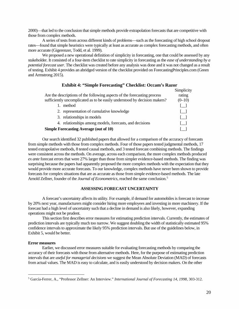
20

2000)—that led to the conclusion that simple methods provide extrapolation forecasts that are competitive with those from complex methods.

A series of tests from across different kinds of problems—such as the forecasting of high school dropout rates—found that simple heuristics were typically at least as accurate as complex forecasting methods, and often more accurate (Gigerenzer, Todd, et al. 1999).

We proposed a new operational definition of simplicity in forecasting, one that could be assessed by any stakeholder. It consisted of a four-item checklist to rate simplicity in forecasting as the ease of understanding by a potential forecast user. The checklist was created before any analysis was done and it was not changed as a result of testing. Exhibit 4 provides an abridged version of the checklist provided on ForecastingPrinciples.com (Green and Armstrong 2015).

Exhibit 4: “Simple Forecasting” Checklist: Occam’s Razor

Are the descriptions of the following aspects of the forecasting process sufficiently uncomplicated as to be easily understood by decision makers?

Simplicity rating (0–10)

1. method [__] 2. representation of cumulative knowledge [__] 3. relationships in models [__] 4. relationships among models, forecasts, and decisions [__]

Simple Forecasting Average (out of 10) [__]

Our search identified 32 published papers that allowed for a comparison of the accuracy of forecasts from simple methods with those from complex methods. Four of those papers tested judgmental methods, 17 tested extrapolative methods, 8 tested causal methods, and 3 tested forecast combining methods. The findings were consistent across the methods. On average, across each comparison, the more complex methods produced ex ante forecast errors that were 27% larger than those from simpler evidence-based methods. The finding was surprising because the papers had apparently proposed the more complex methods with the expectation that they would provide more accurate forecasts. To our knowledge, complex methods have never been shown to provide forecasts for complex situations that are as accurate as those from simple evidence-based methods. The late Arnold Zellner, founder of the Journal of Econometrics, reached the same conclusion.5

ASSESSING FORECAST UNCERTAINTY

A forecast’s uncertainty affects its utility. For example, if demand for automobiles is forecast to increase

by 20% next year, manufacturers might consider hiring more employees and investing in more machinery. If the forecast had a high level of uncertainty such that a decline in demand is also likely, however, expanding operations might not be prudent.

This section first describes error measures for estimating prediction intervals. Currently, the estimates of prediction intervals are typically much too narrow. We suggest doubling the width of statistically estimated 95% confidence intervals to approximate the likely 95% prediction intervals. But use of the guidelines below, in Exhibit 5, would be better.

Error measures

Earlier, we discussed error measures suitable for evaluating forecasting methods by comparing the accuracy of their forecasts with those from alternative methods. Here, for the purpose of estimating prediction intervals that are useful for managerial decisions we suggest the Mean Absolute Deviation (MAD) of forecasts from actual values. The MAD is easy to calculate, and is easily understood by decision makers. On the other

5 García-Ferrer, A., “Professor Zellner: An Interview.” International Journal of Forecasting 14, 1998, 303-312.

21

hand, the commonly used Root Mean Square Error (RMSE) measure should be avoided as it cannot be related to benefits.

For forecasting problems that are expected to involve asymmetric errors—i.e., negative errors are larger than positive errors, or vice versa—calculate the logarithms of the forecast and actual values and calculate the errors using the logged values. Use those errors to estimate prediction intervals, and then convert the bounds of the intervals back to actual values (p. 281, Armstrong and Collopy 2001).

Loss functions can also be asymmetric. For example, the losses due to a forecast that is too low by 50 units may differ from the losses if a forecast is too high by 50 units. Asymmetric errors are, however, a problem for the planner, not the forecaster: the planner must assess the damages resulting from positive versus negative errors. Methods to forecast uncertainty

Exhibit 5 presents a checklist of methods to forecast uncertainty. The checklist includes four valid methods to use, and two commonly used but invalid methods to avoid.

Exhibit 5: Methods to Forecast Uncertainty Checklist

1. Use empirical prediction intervals or likelihoods estimated from out-of-sample tests

2. Decompose errors by source in order to estimate the uncertainty of each

3. Use structured judgment to estimate prediction intervals or likelihoods

4. Combine alternative valid estimates of uncertainty

5. Avoid using statistical fit with historical data to assess uncertainty

6. Avoid using tests of statistical significance to assess uncertainty 1. Use empirical prediction intervals or likelihoods estimated from out-of-sample tests

Traditional statistical confidence intervals estimated from historical data are usually too narrow. One study showed that the percentage of actual values that fell outside the 95% confidence intervals for extrapolation forecasts was often greater than 50% (Makridakis, Hibon, Lusk, and Belhadjali 1987).

In order to provide forecast users with useful information on forecast uncertainty, there is no alternative to estimating empirical prediction intervals based on out-of-sample forecast errors. To that end, simulate the actual forecasting procedure as closely as possible and use the distribution of the errors of the resulting forecasts to assess uncertainty. Tashman (2000) provides guidance on out-of-sample testing. For more on estimating prediction intervals, see Chatfield (2001).

When analyzing time-series forecast errors, use successive updating to increase the number of predictions. If sufficient validation data are not available, consider using data from analogous situations. 2. Decompose errors by source in order to estimate the uncertainty of each

Most forecasting problems are subject to several sources of forecast error. To help ensure that all possible errors are accounted for, consider decomposing errors by source of error to estimate each, then combine the estimates. For example, when polling to predict the outcomes of political elections, survey researchers report only the error expected due to random variation based on the size of the sample. Response and non-response bias errors are ignored. As a consequence, the 95% confidence intervals reported for polls are about half as large as they should be (Buchanan 1986). In other words, decision-makers should double political polls’ confidence intervals to obtain more realistic estimates of the prediction intervals.

When uncertainty is high—such as with surveying citizens to forecast their behavior in response to changes in government regulations—response error is likely to be particularly high due to survey respondents’ lack of self-knowledge about how they make decisions (see Nisbett and Wilson 1977). Non-response can also be a large source of error because people who are most affected by the topic of the survey are more likely to

22

respond. While the latter error can be reduced to some extent by the “extrapolation-across-waves” method (Armstrong and Overton 1977), forecasters still need to consider that source of error when assessing uncertainty.

As with analyses of survey responses, regression models’ diagnostic statistics ignore key sources of uncertainty such as the omission of key variables, the difficulty in controlling or forecasting the causal variables, inability to make accurate forecasts of the causal variables, and the difficulty of assessing the relative importance of causal variables that are correlated with one another. These problems are magnified when analysts strive for a close fit with historical data, and even more so when data-mining techniques are used to achieve a close fit. 3. Use structured judgment to estimate prediction intervals or likelihoods

One common judgmental approach to assessing uncertainty is to ask experts to express their confidence in their own judgmental forecasts in the form of 95% prediction intervals. One concern with that approach is that experts are typically overconfident about the accuracy of their forecasts. For example, an analysis of judgmental confidence intervals for economic forecasts from 22 economists over 11 years found that outcomes were within the range of their 95% confidence intervals only 57% of the time (McNees 1992). Another study tracked members of a ten-year panel who provided 13,300 estimates of expected stock market returns by company; the actual returns were within the executives’ 80% confidence intervals only 36% of the time (Ben-David, et al. 2013).

A number of structured approaches can improve the calibration of judgmental forecasts. Ensure that the judgments are obtained from many experts and obtain independent anonymous estimates. The Delphi technique can be used for that purpose. Ask experts to list all sources of uncertainty, and all reasons why their forecasts might be wrong. That approach was shown to be effective by Arkes (2001).

Finally, to improve the calibration of forecasters’ estimates of uncertainty in the future, ensure that they receive timely, accurate, frequent, and well-summarized information on what actually happened and reasons why their forecasts were right or wrong. For example, weather forecasters use such procedures, and their forecasts are well-calibrated for a few days ahead: When they say that there is a 40% chance of rain, rain falls 40% of the time on average (Murphy and Winkler 1984). 4. Combine alternative valid estimates of uncertainty The logic behind combining uncertainty estimates is the same as that for combining forecasts. Thus, the estimates of uncertainty based on combined estimates can never be worse than the typical estimate, and the combined estimate will always be better than the typical estimate as long as bracketing of the uncertainty estimates occurs. 5. Avoid using statistical fit with historical data to assess uncertainty

In a study using data consisting of 31 observations on 30 variables, stepwise regression was used with a rule that only variables with a t-statistic greater than 2.0 would be included in the model. The data were from a book of random numbers. Despite that, the stepwise method delivered an eight-variable regression model with good statistical fit—an R2 of 0.85 adjusted for degrees of freedom (Armstrong 1970).

Measures of statistical fit do not provide useful information about out-of-sample predictive validity (Armstrong 2001d). Experiments testing analysts’ interpretation of standard statistical fit information on regression models found that 72% grossly underestimated the uncertainty of forecasts associated with changes to the model’s causal (policy) variable (Soyer and Hogarth 2012). Further discussion on why forecasters should avoid such measures as adjusted R2 is provided in Armstrong (2001e). 6. Avoid using tests of statistical significance to assess uncertainty

Statistical significance tests do not provide estimates of forecast uncertainty. Attempts to use them in that way will likely lead to confusion and poor decision making. Experimental studies over more than half a century support that conclusion (e.g., see Ziliak and McCloskey 2008; Hubbard 2016; and Armstrong and Green 2018).

One experiment presented leading researchers with a treatment difference between two drugs, as well as a “p-value” for the difference, and asked them which of the drugs they would recommend to a potential patient. When the difference in the effects of treatments was large but reported to be p > 0.05, nearly half responded that

23

they would advise that there was no difference between the two drugs. By contrast, when the difference between the treatment effects was small but reported to be statistically significant (p < 0.05), 87% of the respondents replied that they would advise taking the drug (McShane and Gal 2015). Many of those teaching statistics also failed to draw logical conclusions as was shown in another experiment by McShane and Gal (2017).

Errors in interpretation of findings due to the provision of statistical significance information have led to poor decisions. Hauer (2004) described the harm caused by decisions related to automobile traffic safety, such as the “right-turn-on-red” policy. Ziliak and McCloskey (2008) provide other examples.

To our knowledge, no scientific study has shown that statistical significance testing has led to better forecasts, decisions, or scientific contributions. Schmidt (1996) offered this challenge: “Can you articulate even one legitimate contribution that significance testing has made (or makes) to the research enterprise (i.e., any way in which it contributes to the development of cumulative scientific knowledge)?” Schmidt and Hunter (1997) stated that no such cases have been reported, and they repeated the challenge, as we have and hereby do again.

DISCUSSION

The accumulation of scientific knowledge about forecasting over the past century enables improvements in forecast accuracy. Regrettably, that knowledge is often ignored, and forecasting practice appears to be in decline. There are two related reasons: first, advocacy research has tended to replace objective forecasting; and second, an unsupported faith in data models has resulted in forecasters ignoring cumulative knowledge about causal relationships and validated forecasting methods (Armstrong and Green 2018).

What recourse do clients and citizens have when they make decisions on the basis of forecasts that turn out to be inaccurate? The answer has traditionally been that there is none, because it has been impossible to distinguish between forecasts that were wrong due to random or unpredictable changes in the situation and those that were wrong due to the forecaster’s failure to follow evidence-based procedures. This paper follows in the footsteps of medicine, engineering, and aviation by providing checklists that can be used to hold forecasters—including scientists who make forecasts, and public policy makers—responsible if they fail to follow evidence-based forecasting procedures.

Forecasters can use the checklists to improve the accuracy of their forecasts and, by communicating that they have followed the checklists, protect themselves from claims against them. Forecasters who follow the checklists might also—as do medical practitioners—obtain protection against damage claims by arranging insurance on the understanding that they follow the forecasting procedures required by the checklists.

Science requires that the predictive validities of hypotheses and new findings are tested. Milton Friedman (1953) viewed out-of-sample predictive validity testing of competing hypotheses as an essential element of economics as a social science. The checklists in this paper can help scientists to design such tests.

CONCLUSIONS

Forecasting practice can be improved such that the accuracy of forecasts upon which decision makers in business and public policy depend is greatly increased. The best way to achieve that objective is to require forecasters to comply with evidence-based checklists.

Exhibit 1, the Forecasting Methods Application Checklist, lists 15 individual evidence-based forecasting methods. The use of those methods substantially improves the ex ante accuracy of forecasts relative to forecasts from commonly used methods, including experts’ unaided judgments. Error reductions range from approximately 5%—for damped-trend extrapolation and decomposition by seasonality—to over 50%—for simulated interaction and knowledge models.

Rather than hoping to identify the one best model, forecasters should employ diverse models from different evidence-based methods, and combine the forecasts from them. Doing so reduces the bias than can arise from using a single method and improves reliability by incorporating more knowledge and information. Combining also avoids the risk of making the worst forecast and guarantees that the combined forecast will be more accurate than the typical forecast if, as is likely, any of the forecasts in the combination bracket the outcome.

24

Data models are not suitable for forecasting. In particular, multiple regression approaches violate evidence-based forecasting principles and provide forecasts that are substantially less accurate that those from the methods listed in the Exhibit 1 checklist. Data models can be and are being used to support clients’ and funders’ prior beliefs and preferences to the further detriment of forecast accuracy.

The Golden Rule and Simple Forecasting principles checklists (Exhibits 3 and 4) can help forecasters to implement the evidence-based methods listed in Exhibit 1, and can help forecasters to improve currently used methods in situations where it is not feasible to replace them with evidence-based methods. Following the Golden Rule of Forecasting can help forecasters reduce forecast errors by over half, while ignoring Occam’s Razor is likely to increase errors by around 27%. The principles checklists can also help clients, sponsors, and users to assess whether proper procedures were followed.

Procedures currently used to assess forecast uncertainty mislead analysts, clients, and users into excessive confidence. As a rule of thumb, they are half as uncertain as they should be. Prediction intervals should only be estimated by using out-of-sample testing, as described in the Exhibit 5 checklist.

Clients and other funders who are interested in accurate forecasts should require forecasters to follow the five evidence-based checklists provided in this paper, and should audit the forecasters’ procedures to ensure that they did so. Clients and other forecast stakeholders can use the checklists to assess the worth of forecasts by determining whether they were the product of scientific forecasting procedures.

REFERENCES

Key NS: not cited regarding substantive finding AO: this paper's authors' own paper NF: unable to find email address (including deceased) NR: contact attempted (email sent) but no substantive reply received FD: disagreement over interpretation of findings remains FC: interpretation of findings confirmed in this or in a related paper

Arkes, H. R. (2001). Overconfidence in judgmental forecasting. In J. S. Armstrong (Ed.), Principles of Forecasting (pp. 495–

515). Boston, MA: Kluwer Academic Publishers. FC Armstrong, J. S. (2012a). Predicting job performance: The moneyball factor. Foresight, 25, 31-34. AO Armstrong, J. S. (2012b). Illusions in regression analysis. International Journal of Forecasting 28, 689-694.AO Armstrong, J. S. (2010). Persuasive Advertising: Evidence-based principles. New York: Palgrave Macmillan. AO Armstrong, J. S. (2007a). Significance tests harm progress in forecasting. International Journal of Forecasting, 23, 321–327.

AO Armstrong, J. S. (2007b). Statistical significance tests are unnecessary even when properly done and properly

interpreted: Reply to commentaries, International Journal of Forecasting, 23, 335-336. AO Armstrong, J. S. (2006). Findings from evidence-based forecasting: Methods for reducing forecast error. International

Journal of Forecasting, 22, 583–598. AO Armstrong, J. S. (Ed.) (2001). Principles of Forecasting. Norwell, MA: Kluwer. AO Armstrong, J. S. (2001a). Judgmental bootstrapping: Inferring experts’ rules for forecasting. In J. S. Armstrong (Ed.),

Principles of Forecasting (pp. 171–192). Norwell, MA: Kluwer Academic Publishers. AO Armstrong, J. S. (2001b). Standards and practices for forecasting. In J. S. Armstrong (Ed.), Principles of Forecasting (pp.

679-732). Norwell, MA: Kluwer Academic Publishers. AO Armstrong, J. S. (2001c). Combining forecasts. In J. S. Armstrong (Ed.), Principles of Forecasting (pp. 417-439). Norwell,

MA: Kluwer Academic Publishers. AO Armstrong, J. S. (2001d). Evaluating forecasting methods. In J. S. Armstrong (Ed.), Principles of Forecasting (pp. 443-472.

Norwell, MA: Kluwer Academic Publishers. AO Armstrong, J. S. (1985). Long-Range Forecasting. New York: John Wiley and Sons. AO Armstrong, J. S. (1980). The seer-sucker theory: The value of experts in forecasting. Technology Review, 83, 18-24. AO Armstrong, J. S. (1978). Forecasting with econometric methods: Folklore versus fact. The Journal of Business 51,

549-64. AO Armstrong, J. S. (1970). How to avoid exploratory research. Journal of Advertising Research, 10, No. 4, 27-30. AO

25

Armstrong, J. S., Adya, M., & Collopy, F. (2001). Rule-based forecasting: Using judgment in time-series extrapolation. In J. S. Armstrong (Ed.), Principles of Forecasting (pp. 259–282). Norwell, MA: Kluwer Academic Publishers. AO

Armstrong, J. S., & Andress, J. G. (1970). Exploratory analysis of marketing data: Trees vs. regression. Journal of Marketing Research, 7, 487-492. AO

Armstrong, J. S., & Collopy, F. (2001). Identification of asymmetric prediction intervals through causal forces. Journal of Forecasting, 20, 273–283. AO

Armstrong, J. S., & Collopy, F. (1993). Causal forces: Structuring knowledge for time series extrapolation. Journal of Forecasting, 12, 103–115. AO

Armstrong, J. S., & Collopy, F. (1992). Error measures for generalizing about forecasting methods: Empirical comparisons. International Journal of Forecasting, 8, 69–80. AO

Armstrong, J. S., Collopy, F., & Yokum, T. (2005). Decomposition by causal forces: A procedure for forecasting complex time series. International Journal of Forecasting, 21, 25-36. AO

Armstrong, J. S., & Cuzán, A. G. (2006). Index methods for forecasting: An application to American presidential elections. Foresight: The International Journal of Applied Forecasting, 3, 10-13. AO

Armstrong, J. S., Denniston, W. B., & Gordon, M. M. (1975). The use of the decomposition principle in making judgments. Organizational Behavior and Human Performance, 14, 257-263. AO

Armstrong, J.S., Du, R., Green, K.C., & Graefe, A. (2016). Predictive validity of evidence-based persuasion principles, European Journal of Marketing, 50, 276-293. AO

Armstrong, J.S., & Green, K. C. (2018). Guidelines for science: Evidence and checklists. Working paper, ResearchGate. AO

Armstrong, J.S., Green, K. C., & Graefe, A. (2015). Golden rule of forecasting: Be conservative. Journal of Business Research, 68, 1717–1731. AO

Armstrong, J. S., Morwitz, V., & Kumar, V. (2000). Sales forecasts for existing consumer products and services: Do purchase intentions contribute to accuracy? International Journal of Forecasting, 16, 383–397. AO

Armstrong, J. S., & Overton, T. S. (1977). Estimating nonresponse bias in mail surveys. Journal of Marketing Research 14, 396-402. AO

Armstrong, J. S., & Overton, T. S. (1971). Brief vs. comprehensive descriptions in measuring intentions to purchase. Journal of Marketing Research, 8, 114–117. AO

Armstrong, J. S., & Pagell, R. (2003). Reaping benefits from management research: Lessons from the forecasting principles project, Interfaces, 33, 89-111. AO

Armstrong, J. S., & Patnaik, S. (2009). Using quasi-experimental data to develop empirical generalizations for persuasive advertising. Journal of Advertising Research. 49, 170-175. AO

Armstrong, J. S., & Yokum, T. (1994). Effectiveness of monetary incentives: Mail surveys of multinational professional groups. Industrial Marketing Management, 23, 133-136. AO

Babst, D. V., Gottfredson, D. M., & Ballard, Jr., K. B. (1968). Comparison of multiple regression and configural analysis techniques for developing base expectancy tables. Journal of Research in Crime and Delinquency, 5, 72-80. NF

Batchelor, R., & Dua, P. (1995). Forecaster diversity and the benefits of combining forecasts. Management Science, 41, 68–75. FC

Belvedere, V., & Goodwin, P. (2017). The influence of product involvement and emotion on short-term product demand forecasting. International Journal of Forecasting, 33, 652-661. FC

Ben-David, I., Graham, J. R., & Harvey. C. R. (2013). Managerial miscalibration. The Quarterly Journal of Economics, 128, 1547-1584. FC

Boylan, J. E., Goodwin. P, Mohammadipour, M., & Syntetos, A. A. (2015). Reproducibility in forecasting research. International Journal of Forecasting 3, 79-90. FC

Bradburn, N. M., Sudman, S., & Wansink, B. (2004). Asking Questions: The Definitive Guide to Questionnaire Design – For Market Research, Political Polls, and Social and Health Questionnaires, 2nd Edition. New York: John Wiley & Sons. NS

Brown, R. G. (1962). Smoothing, Forecasting and Prediction of Discrete Time Series. London: Prentice-Hall.NF

Brown, R. G. (1959). Statistical Forecasting for Inventory Control. New York: McGraw-Hill. NF Buchanan, W. (1986). Election predictions: An empirical assessment. Public Opinion Quarterly, 50, 222-227. NF Bunn, D. W., & Vassilopoulos, A. I. (1999). Comparison of seasonal estimation methods in multi-item short-term

forecasting. International Journal of Forecasting, 15, 431–443. FC Burgess, E. W. (1936). Protecting the public by parole and by parole prediction, Journal of Criminal Law and

Criminology, 27, pp. 491–502. NF Cerf, C., & Navasky, V. (1998). The Experts Speak. New York: Villard. NS

26

Chamberlin, T. C. (1890). The method of multiple working hypotheses. Reprinted in 1965 in Science, 148, 754-759.NF

Chatfield, C. (2001). Prediction intervals for time series. In J. S. Armstrong (Ed.), Principles of Forecasting (pp. 475–494). Norwell, MA: Kluwer Academic Publishers. FC

Chen, C., Twycross, J., & Garibaldi, J. M. (2017). A new accuracy measure based on bounded relative error for time series forecasting. PLoS ONE, 12(3): e0174202. https://doi.org/10.1371/journal.pone.0174202 FC

Collopy, F., Adya, M., & Armstrong, J. S. (2001). Expert systems for forecasting. In J. S. Armstrong (Ed.), Principles of Forecasting (pp. 285–300). Norwell, MA: Kluwer Academic Publishers. AO

Collopy, F., & Armstrong, J. S. (1992). Rule-based forecasting: Development and validation of an expert systems approach to combining time-series extrapolations. Management Science, 38, 1394–1414. AO

Coulson, M., Healey, M., Fidler, F., & Cumming, G. (2010). Confidence intervals permit, but do not guarantee, better inference than statistical significance testing. Frontiers in Psychology, 1(26), 1-9. doi: 10.3389/fpsyg.2010.00026 FC

Cox, J. E., & Loomis, D. G. (2001). Diffusion of forecasting principles through books. In J. S. Armstrong (Ed.), Principles of Forecasting (pp. 633-–649). Norwell, MA: Kluwer Academic Publishers. NR

Czerlinski, J., Gigerenzer, G., & Goldstein, D. G. (1999). How good are simple heuristics? In G.Gigerenzer, P. M. Todd, & the ABC Research Group (Eds.), Simple heuristics that make us smart (pp. 97-118). Oxford University Press. FC

Dana, J., & Dawes, R. M. (2004). The superiority of simple alternatives to regression for social science predictions. Journal of Educational and Behavioral Statistics, 29 (3), 317-331.FC

Dawes, R. M. (1971). A case study of graduate admissions: Application of three principles of human decision making. American Psychologist, 26, 180-188.NF

Dawes, R. M., & Corrigan, B. (1974). Linear models in decision-making. Psychological Bulletin, 81, 95-106. NF Dielman, T. E. (1986). A comparison of forecasts from least absolute value and least squares regression. Journal of

Forecasting, 5, 189-195. NS Dielman, T. E. (1989). Corrections to A comparison of forecasts from least absolute value and least squares regression.

Journal of Forecasting, 8, 419-420. NS Dillman, D. A., Smyth J. D., & Christian, L. M. (2014). Internet, Mail, and Mixed-Mode Surveys: The Tailored Design

Method. (4th ed.). Hoboken, NJ: John Wiley. NS Edmundson, R. H. (1990). Decomposition; A strategy for judgmental forecasting. Journal of Forecasting, 9, 305-

314.NF Einhorn, H. J. (1972). Alchemy in the behavioral sciences. Public Opinion Quarterly, 36, 367-378.NF Einhorn, H. J., & Hogarth, R. (1975). Unit weighting schemes for decision making. Organizational Behavior and

Human Performance, 13, 171-192. FC Fildes, R., & Goodwin, P. (2007). Against your better judgment? How organizations can improve their use of management

judgment in forecasting. Interfaces, 37, 570-576. FC Fildes, R., Goodwin, P., Lawrence, M., & Nikolopoulos, K. (2009). Effective forecasting and judgmental adjustments: An

empirical evaluation and strategies for improvement in supply-chain planning. International Journal of Forecasting, 25, 3–23. FC

Fildes, R., & Hastings, R. (1994). The organization and improvement of market forecasting, Journal of the Operational Research Society, 45, 1-16. FC

Franses, P. H. (2014). Expert adjustments of model forecasts: theory, practice and strategies for improvement. Cambridge, U.K.: Cambridge University Press. FC

Friedman, M. (1953). The methodology of positive economics, from Essays in Positive Economics reprinted in Hausman, D. M. (ed.) The philosophy of Economics: An anthology (3rd Ed.), Cambridge: Cambridge University Press, pp. 145-178.

Gardner, E. S., Jr. (2006). Exponential smoothing: The state of the art – Part II (with commentary). International Journal of Forecasting, 22, 637–677. FC

Gigerenzer, G., Todd, P. M., & The ABC Research Group (1999). Simple Heuristics that Make Us Smart. New York: Oxford University Press. FC

Gorr, W., Olligschlaeger, A., & Thompson, Y. (2003). Short-term forecasting of crime. International Journal of Forecasting, 19, 579–594. FC

Graefe, A. (2017a). Political markets. In Arzheimer, K., & Lewis-Beck, M. S. (eds.). The Sage Handbook of Electoral Behavior. Los Angeles: Sage. FC

Graefe, A. (2017b). Prediction market performance in the 2016 U. S. presidential election, Foresight, – The International Journal of Applied Forecasting, 45, 38-42. FC

27

Graefe, A. (2015). Improving forecasts using equally weighted predictors. Journal of Business Research, 68, 1792–1799. FC

Graefe, A. (2014). Accuracy of vote expectation surveys in forecasting elections. Public Opinion Quarterly, 78 (S1): 204–232. FC

Graefe, A. (2011). Prediction market accuracy for business forecasting. In L. Vaughan-Williams (Ed.), Prediction Markets (pp. 87–95). New York: Routledge. FC

Graefe, A., & Armstrong, J. S. (2013). Forecasting elections from voters’ perceptions of candidates’ ability to handle issues. Journal of Behavioral Decision Making, 26, 295-303. DOI: 10.1002/bdm.174. AO

Graefe, A., & Armstrong, J. S. (2012). Predicting elections from the most important issue: A test of the take-the-best heuristic, Journal of Behavioral Decision Making, 25, 41-48. AO

Graefe, A., Armstrong, J. S., & Green, K. C. (2014). Improving causal models for election forecasting: Further evidence on the Golden Rule of Forecasting. APSA 2014 Annual Meeting Paper. AO

Graefe, A., Armstrong, J. S., Jones, R. J., & Cuzan, A. G. (2017). Assessing the 2016 U.S. Presidential Election Popular Vote Forecasts, in The 2016 Presidential Election: The causes and consequences of an Electoral Earthquake. Lexington Books, Lanham, MD. AO

Graefe, A., Armstrong, J. S., Jones, R. J., & Cuzan, A. G. (2014). Combining forecasts: An application to political elections. International Journal of Forecasting, 30, 43-54. AO

Green, K. C. (2005). Game theory, simulated interaction, and unaided judgment for forecasting decisions in conflicts: Further evidence. International Journal of Forecasting, 21, 463–472. AO

Green, K. C., & Armstrong, J. S. (2015). Simple versus complex forecasting: The evidence. Journal of Business Research 68 (8), 1678-1685. AO

Green, K. C., & Armstrong, J. S. (2011). Role thinking: Standing in other people’s shoes to forecast decisions in conflicts, International Journal of Forecasting, 27, 69–80. AO

Green, K. C., & Armstrong, J. S. (2007a). Structured analogies for forecasting. International Journal of Forecasting, 23, 365–376. AO

Green, K. C., & Armstrong, J. S. (2007b). Global warming: Forecasts by scientists versus scientific forecasts. Energy and Environment, 18, 995-1019. AO

Green, K.C., Armstrong, J. S., Du, R., & Graefe, A. (2016). Persuasion principles index: ready for pretesting advertisements. European Journal of Marketing, 50, 317-326. https://doi.org/10.1108/EJM-12-2015-0838

Green, K. C., Armstrong, J. S., & Graefe, A. (2015). Golden rule of forecasting rearticulated: Forecast unto others as you would have them forecast unto you. Journal of Business Research, 68, 1768-1771. AO

Green, K. C., Armstrong, J. S., & Graefe, A. (2007). Methods to elicit forecasts from groups: Delphi and prediction markets compared. Foresight, 8, 17–20. AO

Green, K. C., Armstrong, J. S., & Soon (2009). Validity of climate change forecasting for public policy decision making, International Journal of Forecasting, 25, 826-832. AO

Grove, W. M., Zaid, D. H., Lebow, B. S., Snitz, B. E., & Nelson, C. (2000). Clinical versus mechanical prediction: A meta-analysis. Psychological Assessment, 12, 19-30. FC

Hafenbradl, S., Waeger, D., Marewski, J. N., & Gigerenzer, G. (2016). Applied decision making with fast-and-frugal heuristics. Journal of Applied Research in Memory and Cognition, 5, 215-231. FC

Hales, B. M., & Pronovost, P. J. (2006). The checklist—a tool for error management and performance improvement. Journal of Critical Care, 21, 231-235. NS

Hauer, E. (2004). The harm done by tests of significance. Accident Analysis and Prevention, 36, 495-500. FC Hayes, S. P. Jr. (1936).The inter-relations of political attitudes: IV. Political attitudes and party regularity. The

Journal of Social Psychology, 10, 503-552. NF

Haynes, A. B., et al. (2009). A surgical checklist to reduce morbidity and mortality in a global population. New England Journal of Medicine, 360 (January 29), 491-499. NR

Hogarth, R. M. (1978). A note on aggregating opinions. Organizational Behavior and Human Performance, 21, 40-46. FC Hubbard, R. (2016). Corrupt Research: The Case for Reconceptualizing Empirical Management and Social Science.

New York: Sage. FC Ioannidis, J. P. A. (2005). Why most published findings are false. PLOS Medicine, 2(8): e124. doi:

10.1371/journal.pmed.0020124 NR Jones, R. J., Armstrong, J. S., & Cuzan, A. G. (2007). Forecasting elections using expert surveys: An application to U. S.

presidential elections, MPRA Paper No. 5301. AO Kabat, G. C. (2008). Hyping Health Risks N.Y., N.Y.: Columbia University Press. FC Keogh, E., & Kasetty, S. (2003). On the need for time series data mining benchmarks: A survey and empirical

demonstration. Data Mining and Knowledge Discovery, 7, 349–371. FC

28

Kim, M. S., & Hunter, J. E. (1993). Relationships among attitudes, behavioral intentions, and behavior: A meta-analysis of past research. Communication Research, 20, 331–364. FC

Larrick, R. P., & Soll, J. B. (2006). Intuitions about combining opinions: Misappreciation of the averaging principle. Management Science, 52(1), 111–127. FC

Lin, S., Goodwin, P., & Song, H. (2014). Accuracy and bias of experts’ adjusted forecasts. Annals of Tourism Research, 48, 156-174. FC

Locke, E. A. (1986). Generalizing from Laboratory to Field Settings. Lexington, MA: Lexington Books. FC Lott, J. R., Jr. (2016). The War on Guns. Washington, D.C: Regnery Publishing. FC Lott, J. R., Jr. (2010). More Guns, Less Crime. Third Edition. Chicago, IL: University of Chicago Press. FC Lovallo, D., Clarke, C., & Camerer, C. (2012). Robust analogizing and the outside view: Two empirical tests of case-based

decision making. Strategic Management Journal, 33, 496–512. FC MacGregor, D. G. (2001). Decomposition for judgmental forecasting and estimation. In J. S. Armstrong (Ed.), Principles of

Forecasting (pp. 107–123). Norwell, MA: Kluwer Academic Publishers. FC Makridakis, S. G., Andersen, A., Carbone, R., Fildes, R., Hibon, M., Lewandowski, R., Newton, J., Parzen, E., & Winkler, R.

(1984). The Forecasting Accuracy of Major Times Series Methods. Chichester: John Wiley. FC Makridakis, S. G., Andersen, A., Carbone, R., Fildes, R., Hibon, M., Lewandowski, R., Newton, J. Parzen, E., & Winkler, R.

(1982). The accuracy of extrapolation (time series) methods: Results of a forecasting competition. Journal of Forecasting 1, 111-153. FC

Makridakis, S., Chatfield, C., Hibon, M., Lawrence, M., Mills, T., Ord, K., & Simmons, L. F. (1993). The M-2 Competition: a real-time judgmentally based forecasting study. International Journal of Forecasting, 9, 5–23. FC

Makridakis, S., & Hibon, M. (2000). The M3-Competition: Results, conclusions and implications. International Journal of Forecasting, 16, 451–476. FC

Makridakis, S., & Hibon, M. (1979). Accuracy of forecasting: An empirical investigation (with discussion). Journal of the Royal Statistical Society A, 142, 97–145. FC

Makridakis, S., Hibon, M., Lusk, E., & Belhadjali, M. (1987). Confidence intervals: An empirical investigation of time series in the M-competition. International Journal of Forecasting, 3, 489–508. FC

Mannes, A. E., Soll, J. B., & Larrick, R. P. (2014). The wisdom of select crowds. Journal of Personality and Social Psychology, 107, 276-299. FC

McNees, S. K. (1992). The uses and abuses of ‘consensus’ forecasts. Journal of Forecasting, 11, 703-710. NF McShane, B. B., & Gal, D. (2015). Blinding us to the obvious? The effect of statistical training on the evaluation of

evidence. Management Science, 62, 1707-1718. FC McShane, B. B., & Gal, D. (2017). Rejoinder: Statistical significance and the dichotomization of evidence. Journal

of the American Statistical Association, 112:519, 904-908, DOI: 10.1080/01621459.2017.1323642 FC Meehl, P.E. (1954). Clinical vs. Statistical Prediction, Minneapolis: University of Minnesota Press. NF Miller, D. M., & Williams, D. (2003). Shrinkage estimators of time series seasonal factors and their effect on forecasting

accuracy, International Journal of Forecasting, 19, 669-684. FC Miller, D. M., & Williams, D. (2004). Shrinkage estimators for damping X12-ARIMA seasonals. International

Journal of Forecasting, 20, 529–549. FC

Morwitz, V. G. (2001). Methods for forecasting from intentions data. In J. S. Armstrong (Ed.), Principles of Forecasting (pp. 33–56). Norwell, MA: Kluwer Academic Publishers. FC

Morwitz, V. G., Steckel, J. H., & Gupta, A. (2007). When do purchase intentions predict sales? International, Journal of Forecasting, 23, 347–364. FC

Murphy, A. H., & Winkler, R. L. (1984). Probability forecasting in meteorology, Journal of the American Statistical Association. 79, 489-500. NR

Namboodiri, N. K., & Lalu, N. M. (1971). The average of several simple regression estimates as an alternative to the multiple regression estimate in postcensal and intercensal population estimates: A case study, Rural Sociology, 36, 187-194. . NF

Nikolopoulos, K., Litsa, A., Petropoulos, F., Bougioukos, V., & Khammash, M. (2015). Relative performance of methods for forecasting special events, Journal of Business Research, 68, 1785-1791. FC

Nisbett, R. E., & Wilson, T. D. (1977). Telling more than we can know: Verbal reports on mental processes, Psychological Review, 84, 231-259. FC

Perry, M. J. (2017). 18 spectacularly wrong predictions made around the time of first Earth Day in 1970, expect more this year. AEIdeas, April 20. FC

Pool, I. de S., Abelson, R. P., & Popkin, S. L. (1965). Candidates, Issues and Strategies: A Computer Simulation of the 1960 and 1974 Presidential Elections. Cambridge, MA: MIT Press. NF

Rhode, P. W., & Strumpf, K. S. (2004). Historical presidential betting markets. Journal of Economic Perspectives, 18, 127-141. FC

29

Rowe, G., & Wright, G. (2001). Expert opinions in forecasting role of the Delphi technique. In J. Armstrong (Ed.), Principles of Forecasting (pp. 125–144). Norwell, MA: Kluwer Academic Publishers. FC

Schmidt, F. L. (1996). Statistical significance testing and cumulative knowledge in psychology: Implications for training of researchers. Psychological Methods, 1, 115–129. FC

Schmidt, F. L. (1971). The relative efficiency of regression and simple unit predictor weights in applied differential psychology. Educational and Psychological Measurement, 31, 699-714. FC

Schmidt, F. L., & Hunter, J. E. (1997). Eight common but false objections to the discontinuation of significance testing in the analysis of research data, in Harlow, L. L., Mulaik, S. A. & Steiger, J. H. What if there were no Significance Tests? London: Lawrence Erlbaun. FC

Shamir, J. (1986). Pre-election polls in Israel: Structural constraints on accuracy, Public Opinion Quarterly, 50, 62-75. NR

Sheeran, P. (2002). Intention-behavior relations: A conceptual and empirical review. in W. Stroebe and M. Hewstone, European Review of Social Psychology, 12, 1-36. FC

Simon, J. L. (1996). The Ultimate Resource II: People, Materials, Environment. Princeton, NJ: Princeton University Press. NF

Soyer, E., & Hogarth, R. M. (2012). The illusion of predictability: How regression statistics mislead experts. International Journal of Forecasting, 28, 695-711. FC

Tashman, L. J. (2000). Out-of-sample tests of forecasting accuracy: An analysis and review. International Journal of Forecasting. NS

Tashman, L. J. & Hoover, J. (2001). Diffusion of forecasting principles through software. In J. S. Armstrong (Ed.), Principles of Forecasting (pp. 651–676). Norwell, MA: Kluwer Academic Publishers. NS

Tessier, T. H., & Armstrong, J. S. (2015). Decomposition of time-series by level and change. Journal of Business Research, 68, 1755–1758. AO

Tetlock, P. E. (2005). Expert political judgment: How good is it? How can we know? New Jersey: Princeton University Press. FC

Trapero, J. R., Pedregal, D. J., Fildes, R., & Kourentzes, N. (2013). Analysis of judgmental adjustments in the presence of promotions. International Journal of Forecasting, 29, 234-243. FC

Tukey, J.W. (1962), The future of data analysis. Annals of Mathematical Statistics,33,1-67. NF Vokurka, R. J., Flores, B. E., & Pearce, S. L. (1996). Automatic feature identification and graphical support in rule-

based forecasting: a comparison. International Journal of Forecasting, 12, 495-512. NR Winston, C. (1993). Economic deregulation: Days of reckoning for microeconomists. Journal of Economic

Literature, 31, 1263-1289. FC Wright, M., & Armstrong, J. S. (2008). Verification of citations: Fawlty towers of knowledge. Interfaces, 38, 125-139. AO Yokum, J. T., & Armstrong, J. S (1995). Beyond accuracy: Comparison of criteria used to select forecasting

methods. International Journal of Forecasting, 11, 591-597. AO Ziliak, S. T., & McCloskey, D. N. (2008). The Cult of Statistical Significance: How the Standard Error Costs Us

Jobs, Justice, and Lives. Ann Arbor: The University of Michigan Press. FC Ziliak, S. T., & McCloskey D. N. (2004). Size matters: The standard error of regressions in the American Economic

Review. The Journal of Socio-Economics, 33, 527–546. FC