Forecasting Stock Market Volatility in Central and Eastern European Countries

Journal of ForecastingJ. Forecast. (2011)Published online in Wiley Online Library(wileyonlinelibrary.com) DOI: 10.1002/for.1214

Forecasting Stock Market Volatility inCentral and Eastern European Countries

BARRY HARRISON1* AND WINSTON MOORE2

1 Nottingham Business School, Nottingham Trent University,Nottingham, UK2 Department of Economics, University of the West Indies,Bridgetown, Barbados

ABSTRACTIn recent years, considerable attention has focused on modelling and forecastingstock market volatility. Stock market volatility matters because stock marketsare an integral part of the financial architecture in market economies and play akey role in channelling funds from savers to investors. The focus of this paperis on forecasting stock market volatility in Central and East European (CEE)countries. The obvious question to pose, therefore, is how volatility can be fore-cast and whether one technique consistently outperforms other techniques. Overthe years a variety of techniques have been developed, ranging from the rela-tively simple to the more complex conditional heteroscedastic models of theGARCH family. In this paper we test the predictive power of 12 models to fore-cast volatility in the CEE countries. Our results confirm that models which allowfor asymmetric volatility consistently outperform all other models considered.Copyright © 2011 John Wiley & Sons, Ltd.

KEY WORDS CEE countries; stock market; volatility

INTRODUCTION

In recent years, considerable attention has focused on modelling and forecasting of stock marketvolatility. Stock market volatility matters because stock markets are an integral part of the financialarchitecture in market economies and play a key role in channelling funds from savers to investors. Acertain amount of volatility is, of course, a natural recurring feature of stock market prices as fundsare allocated among competing users. However, excessive volatility can impair the smooth function-ing of the stock market and cause problems for firms seeking to raise risk capital and for the widermacroeconomy in general.

A major reason why the literature has focused on volatility is that it is an important mea-sure of risk and plays a crucial role in portfolio management, option pricing and market regu-lation (see Poon and Granger, 2003, for a survey). For example, portfolio management stresses

* Correspondence to: Barry Harrison, Nottingham Business School, Nottingham Trent University, Burton Street, NottinghamNGI 4BU, UK. E-mail: [email protected]

Copyright © 2011 John Wiley & Sons, Ltd.

B. Harrison and W. Moore

the necessity of balancing risk against expected return. Since a rise in volatility is taken to implygreater risk, this might discourage risk taking for a given expected return and lead investorsto seek less risky assets. The overall effect of this, as noted by Guo (2002), is to increase thecost of capital to firms seeking to raise additional funds through an issue of stock. This couldpotentially impact on small firms and especially new firms as investors gravitate towards pur-chasing stock in larger and more well-established firms. More generally, if the cost of capitalrises as investor preferences shift towards less risky assets in response to a perceived increase involatility, this will also have implications for the macroeconomy since it is likely to discourageinvestment.

Changing equity prices cause changes in household wealth and there are good theoretical reasonswhy this might also impact on the macroeconomy through its effect on consumption spending. Test-ing this effect has yielded mixed results. Hall (1978) has argued that lagged stock prices are importantin predicting future consumer spending. Other studies also find support for a link between changingequity prices and consumption (see, for example, Campbell, 2000; Kiley, 2000; Davis and Polumbo,2001; Dynan and Maki, 2001). Stevans (2004) has shown that changes in wealth resulting from unan-ticipated changes in the value of equity holdings begin a process whereby households alter consump-tion growth in order to close the gap between actual and target spending. Bernanke and Gertler (1999)have argued that changes in asset prices impact on the real economy through the ‘balance sheetchannel’.

Most of the literature on volatility has focused on the developed stock markets of Europe,the USA and Japan. Only a few investigations have been carried out into volatility in theemerging stock markets of Central and Eastern Europe (CEE) (see, for example, Harvey et al.,1997; Gilmore and McManus, 2001; Kash-Haroutounian and Price, 2001; Poshakwale andMurinde, 2001; Murinde and Poshakwale, 2002; Appiah-Kusi and Menyah, 2003; Salomonsand Grootveld, 2003). In general, these studies conclude that stock market volatility in CEEmarkets tends to be relatively high compared with developed stock markets. One reason forthis is that CEE markets are still comparatively young and, in terms of market capitalisation,volume traded and number of listed companies, are growing at a greater rate than developedmarkets.

The focus of this paper is on forecasting stock market volatility in CEE countries. Financetheory argues that returns ought to be higher where volatility is higher. Since, as noted above,volatility tends to be higher in CEE markets than in more fully developed markets, it follows thatif volatility can be forecast it might be possible to make some general predictions about returnbehaviour. This is important because Harrison and Moore (2009) have argued that CEE marketsdisplay relatively weak co-movement with the developed markets of London and Frankfurt andtherefore offer opportunities for portfolio diversification. The obvious question to pose, there-fore, is how volatility can be forecast and whether one technique consistently outperforms othertechniques. Over the years a variety of techniques have been developed ranging from the rel-atively simple to the more complex conditional heteroscedastic models of the GARCH family(see, for example, Andersen et al., 2006a,b, for a review of the literature). In this paper, we testthe predictive power of 12 models to forecast volatility in the CEE countries. Our results con-firm that models that allow for asymmetric volatility consistently outperform all other modelsconsidered.

The rest of this paper is organised as follows. The next section provides a description of the dataand the third section reviews the models used to test volatility. The fourth section reports our resultsand the fifth section provides a summary and conclusions.

Copyright © 2011 John Wiley & Sons, Ltd. J. Forecast. (2011)DOI: 10.1002/for

Forecasting Stock Market Volatility in CEE Countries

DATA

This study uses daily observations on 10 stock exchanges in CEE countries (Bulgaria, Czech Repub-lic, Estonia, Hungary, Latvia, Lithuania, Poland, Romania, Slovenia and Slovak Republic) cover-ing the period 1991–2008. The series were obtained from Datastream International. Stock marketvolatility is approximated by the squared residuals from an ARMA(1,1) model with a linear trend.The ARMA model is selected using the Akaike information criterion and the parameters of theautoregressive (AR) and moving average (MA) were statistically significant in all regressions.

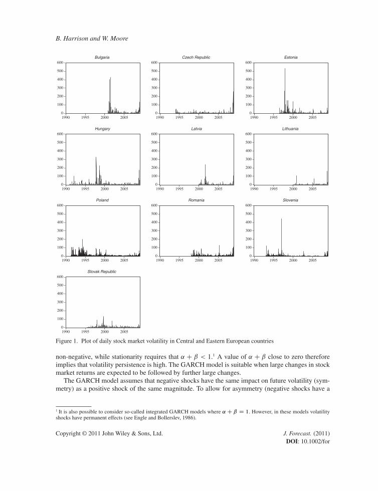
Figure 1 provides a plot of volatility for each country and the descriptive statistics are providedin Table I. The figures reveal that stock market volatility is characterised by volatility clustering: ashock is likely to be followed by other (smaller) shocks. These volatility clusters correspond to thepeaks and troughs of the returns series. Over the sample period considered, the stock exchanges inBulgaria and Poland were the most volatile. Mean volatility on these two stock exchanges was 3.4and 3.6, compared to 2.1 for the other stock markets in our study. Of the CEE countries investigated,Lithuania, the Slovak Republic and Slovenia were the least volatile. Corroborating evidence regardingthe volatility of CEE exchanges can also be obtained by examining Figure 1.

As is usual with financial data, the distribution of returns appears to be non-normal, with estimatedskewness for the volatility series well above zero. In addition, the measure of excess kurtosis for allthe exchanges deviates significantly from that expected for observations drawn from a normal distri-bution. Non-normality is confirmed by the significance of the Jarque–Bera statistic (not reported herebut available from the authors upon request).

VOLATILITY MODELS

One simple approach that can be employed to forecast volatility is to assume that n-step-ahead condi-tional variance is its past n-month average. This naïve model (NVOL) can be estimated by regressingthe realised volatility on a constant. Thus the n-step-ahead forecast is given as

htCn D h (1)

This naïve approach to forecasting volatility, however, does not allow forecast volatility tochange given historical information. GARCH models, introduced by Engle (1982) and generalised byBollerslev (1986), Engle and Bollerslev (1986) and Taylor (1986), are specifically designed to modeland forecast conditional variances. Volatility is modelled as a function of past values of the dependentvariable and independent or exogenous variables.

In general form, the GARCH(p,q) model can be written as

�2t D$ C

pXjD1

˛j "2t�j C

qXjD1

ˇj�2t�j (3)

where equation (3) states that the conditional variance of stock market returns depends on some con-stant ($), the previous period’s squared random component of stock market returns (referred to asARCH effects or the short-run persistence of shocks) and the previous period’s variance (the contri-bution of shocks to long-run persistence, ˛ C ˇ). Non-negativity of �2t requires that $ , ˛ and ˇ are



0

100

200

300

400

500

600

1990 1995 2000 2005

Bulgaria

0

100

200

300

400

500

600

1990 1995 2000 2005

Czech Republic

0

100

200

300

400

500

600

1990 1995 2000 2005

Estonia

0

100

200

300

400

500

600

1990 1995 2000 2005

Hungary

0

100

200

300

400

500

600

1990 1995 2000 2005

Latvia

0

100

200

300

400

500

600

1990 1995 2000 2005

Lithuania

0

100

200

300

400

500

600

1990 1995 2000 2005

Poland

0

100

200

300

400

500

600

1990 1995 2000 2005

Romania

0

100

200

300

400

500

600

1990 1995 2000 2005

Slovenia

0

100

200

300

400

500

600

1990 1995 2000 2005

Slovak Republic

Figure 1. Plot of daily stock market volatility in Central and Eastern European countries

non-negative, while stationarity requires that ˛ C ˇ < 1.1 A value of ˛ C ˇ close to zero thereforeimplies that volatility persistence is high. The GARCH model is suitable when large changes in stockmarket returns are expected to be followed by further large changes.

The GARCH model assumes that negative shocks have the same impact on future volatility (sym-metry) as a positive shock of the same magnitude. To allow for asymmetry (negative shocks have a

1 It is also possible to consider so-called integrated GARCH models where ˛C ˇ D 1. However, in these models volatilityshocks have permanent effects (see Engle and Bollerslev, 1986).



Tabl

eI.

Des

crip

tive

stat

istic

sof

vola

tility

Stat

istic

Bul

gari

aC

zech

Est

onia

Hun

gary

Lat

via

Lith

uani

aPo

land

Rom

ania

Slov

enia

Slov

akR

epub

licR

epub

lic

Mea

n3.

438

1.90

72.

764

2.66

02.

309

1.12

13.

603

2.89

61.

536

1.50

9M

edia

n0.

323

0.35

20.

264

0.43

70.

262

0.17

40.

565

0.58

70.

144

0.16

8M

axim

um42

7.79

626

2.66

053

6.40

832

7.13

524

0.07

016

0.12

320

2.15

312

8.81

644

2.58

413

1.98

8M

inim

um0.

000

0.00

00.

000

0.00

00.

000

0.00

00.

000

0.00

00.

000

0.00

0St

anda

rdde

viat

ion

18.3

087.

912

14.4

7210

.968

10.3

175.

503

10.7

438.

079

9.05

34.

796

Skew

ness

16.2

7817

.409

20.6

3814

.005

12.0

1017

.558

6.78

87.

366

31.3

0011

.458

Kur

tosi

s32

7.21

043

0.97

063

4.64

528

1.67

319

9.58

740

4.22

466

.213

76.0

2013

99.1

6222

7.44

2O

bser

vatio

ns21

1138

8332

5546

6823

2123

2045

9028

4041

4034

95A

RC

Hte

st(F

-sta

tistic

)15

6.59

346

7.62

681

.509

774.

125

559.

958

351.

798

144.

290

494.

650

561.

471

17.9

15[0

.000

][0

.000

][0

.000

][0

.000

][0

.000

][0

.000

][0

.000

][0

.000

][0

.000

][0

.000

]

Not

e:p

-val

ueis

give

nin

squa

rebr

acke

ts.



larger impact on future volatility than positive shocks), Nelson’s (1991) exponential GARCH model(EGARCH) can be employed. This model is given by

log.�2t /D$ CqXjD1

ˇj log.�2t�j /CpXjD1

˛j

ˇ̌ˇ̌ "t�j�t�j

ˇ̌ˇ̌C

rXjD1

�j"t�j

�t�j(4)

The EGARCH model is asymmetric as long asPj

˛j ¤ 0. WhenPj

�j < 0, then positive shocks

generate less volatility than negative shocks. Asymmetry can also be modelled using the thresholdGARCH model introduced independently by Zakoïan (1994) and Runkle et al. (1993). In this case,the specification for the conditional variance is given by

�2t D$ C

pXjD1

˛j "2

t�j C

qXjD1

ˇj�2

t�j C

rXjD1

�j "2

t�j�t�j (5)

where �t�k D 1 if "t<0, and 0 otherwise. In this framework, positive and negative shocks have differ-ential effects on the conditional variance: �j>0 would imply that negative shocks increase volatilityand �j D 0 implies that shocks are symmetric.

Asymmetry can also be modelled using the power ARCH (PARCH) specification introduced byDing et al. (1993). In the PARCH framework the power parameter ı is estimated rather than imposed,and optional parameters are added to capture asymmetry:

�ıt D$ C

pXjD1

˛j .j"t�j j � �j "t�j /ı C

qXjD1

ˇj�ı

t�j (6)

where ı > 0, j�j j � 1 for j D 1, : : : , r , �j D 0 for all j > r and r � p. As in the previous models,shocks are asymmetric if �j D 0.

Rather than assume that the conditional variance shows mean reversion to $ , which is constantfor all t, following Engle and Patton (2001) the component GARCH model can be utilised to allowfor mean reversion to a varying level, mt . Using a GARCH(1,1) model, the component GARCH(CGARCH) can be expressed as

�2t �mt D$ C ˛."2

t�1 �$/C ˇ.�2

t�1 �$/

mt D ! C �.mt�1 �!/C �."2

t�1 � �2

t�1/ (7)

The CGARCH approach would be appropriate if economic policies can result in reducedstock market volatility. One can also estimate the CGARCH model with a threshold, denoted byCGARCHT.

FORECASTING STOCK MARKET VOLATILITY

Comparison criteriaA number of criteria exist for evaluating the forecasting performance of volatility models (see Lopez,2001, for a survey of these approaches). Each method has its own drawbacks, so, rather than choosebetween the approaches, the authors choose six loss functions:

MSE1D n�1nXtD1

.�t � ht/2 (8)



MSE2D n�1nXtD1

��2t � h

2

t

�2(9)

QLIKED n�1nXtD1

�log.h2t /C �

2

t =h2

t

�(10)

R2LOGD n�1nXtD1

�log.�2t =h

2

t /�2

(11)

MAD1D n�1nXtD1

j�t � ht j (12)

MAD2D n�1nXtD1

ˇ̌�2t � h

2

t

ˇ̌(13)

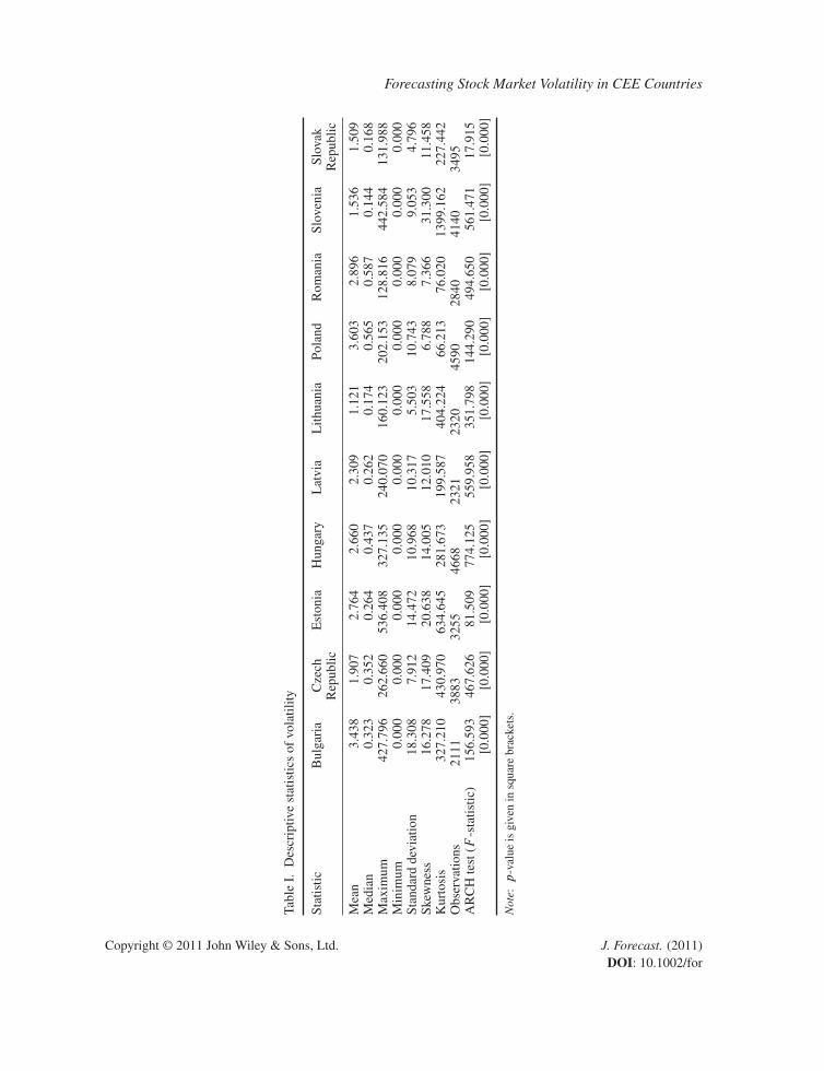
Equations (8) and (9) are the usual mean squared error criteria. The metric QLIKE is the lossimplied by a Gaussian likelihood, while the R2LOG loss function penalises volatility forecasts asym-metrically in low-volatility and high-volatility periods. The final two criteria (equations (12) and (13))are the mean absolute deviation, which tend to be more robust in the presence of outliers than the MSEcriteria.

To evaluate the hypothesis of whether some simple model is as good as any of the more compli-cated models in terms of expected loss, the Diebold and Mariano (1995) model (DM) is employed.The DM provides a useful framework within which to test relatively simple models (for exampleGARCH(1,1)) against more complex alternatives. The test compares a sequence of forecasts frommodel k,h2tC1, : : : , h

2tCn, to the conditional variance, O�2tC1, : : : , O�

2tCn, using a loss function L. Let the

first model, k D 0, be the benchmark model that is compared to the other models, k D 1, : : : , q. Theforecast error function can be calculated asLt D g.ektjk>0/�g.e0t/. The null hypothesis for forecastaccuracy is that E.Lt/ D 0; that is, the forecast error for model k is not significantly different fromthat of the benchmark model.

Defining the mean forecast difference as NL D n�1PLt , the tests take the h-step-ahead

forecasts as autocorrelated up to lag h, and zero thereafter. The variance for NL is estimated as�. NL/ � n�1Œ�0 C 2

Ph�1

sD1�s�, where �s the autocovariance of the loss function, is calculated by

b� s D n�1Pn

tDsC1.Lt � NL/.Lt�h � NL/. The DM test statistic can then be calculated as

DMD Œ�. NL/��1=2 NL (15)

The DM statistic is N.0, 1/ and the variance is the Newey–West robust estimate.

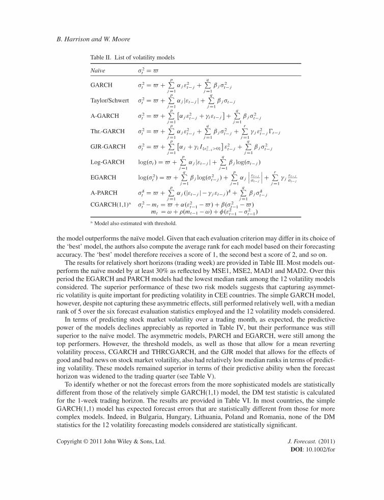
Out-of-sample forecast resultsAll the empirical models outlined above and summarized in Table II, are used to provide out-of-sample forecasts for the period 1 January 2008 to 25 November 2008. The predictions from thesemodels are then compared over weekly, monthly and quarterly trading horizons using the six com-parison criteria outlined earlier (MSE1, MSE2, R2LOG, QLIKE, MAE1, MAE2). Relative forecastevaluation statistics—the forecast evaluation statistic of the model under consideration as a ratio ofthat for the naïve model—are averaged across the CEE countries. A value less than one suggests that



Table II. List of volatility models

Naïve �2t D$

GARCH �2t D$ CpPjD1

˛j "2t�jC

qPjD1

ˇj�2t�j

Taylor/Schwert �2t D$ CpPjD1

˛j j"t�j j CqPjD1

ˇj�t�j

A-GARCH �2t D$ CpPjD1

�˛j "

2t�jC �i"t�j

�C

qPjD1

ˇj�2t�j

Thr.-GARCH �2t D$ CpPjD1

˛j "2t�jC

qPjD1

ˇj�2t�jC

rPjD1

�j "2t�j�t�j

GJR-GARCH �2t D$ CpPjD1

�˛j C �iIf"2t�1>0g

�"2t�jC

qPjD1

ˇj�2t�j

Log-GARCH log.�t /D$ CpPjD1

˛j j"t�j j CqPjD1

ˇj log.�t�j /

EGARCH log.�2t /D$ CqPjD1

ˇj log.�2t�j/C

pPjD1

˛j

ˇ̌ˇ "t�j�t�j

ˇ̌ˇC rP

jD1

�j"t�j

�t�j

A-PARCH �ıt D$ CpPjD1

˛j .j"t�j j � �j "t�j /ı C

qPjD1

ˇj�ıt�j

CGARCH(1,1)a �2t �mt D$ C ˛."2t�1 �$/C ˇ.�

2t�1 �$/

mt D ! C �.mt�1 �!/C �."2t�1 � �

2t�1/

a Model also estimated with threshold.

the model outperforms the naïve model. Given that each evaluation criterion may differ in its choice ofthe ‘best’ model, the authors also compute the average rank for each model based on their forecastingaccuracy. The ‘best’ model therefore receives a score of 1, the second best a score of 2, and so on.

The results for relatively short horizons (trading week) are provided in Table III. Most models out-perform the naïve model by at least 30% as reflected by MSE1, MSE2, MAD1 and MAD2. Over thisperiod the EGARCH and PARCH models had the lowest median rank among the 12 volatility modelsconsidered. The superior performance of these two risk models suggests that capturing asymmet-ric volatility is quite important for predicting volatility in CEE countries. The simple GARCH model,however, despite not capturing these asymmetric effects, still performed relatively well, with a medianrank of 5 over the six forecast evaluation statistics employed and the 12 volatility models considered.

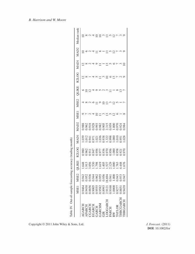
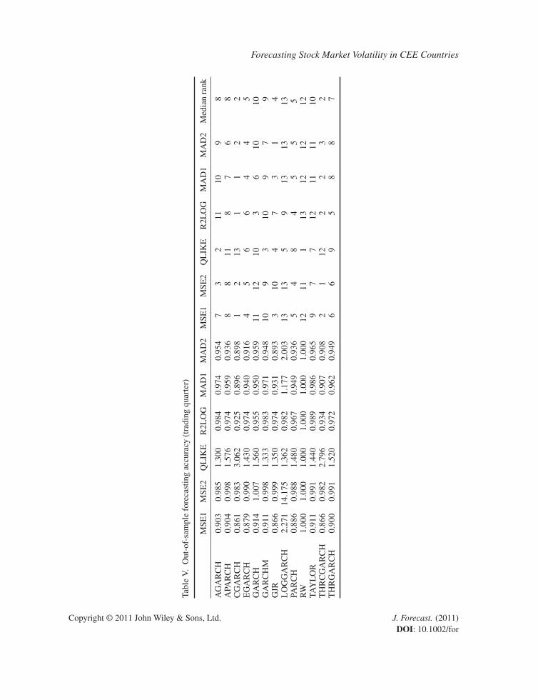
In terms of predicting stock market volatility over a trading month, as expected, the predictivepower of the models declines appreciably as reported in Table IV, but their performance was stillsuperior to the naïve model. The asymmetric models, PARCH and EGARCH, were still among thetop performers. However, the threshold models, as well as those that allow for a mean revertingvolatility process, CGARCH and THRCGARCH, and the GJR model that allows for the effects ofgood and bad news on stock market volatility, also had relatively low median ranks in terms of predict-ing volatility. These models remained superior in terms of their predictive ability when the forecasthorizon was widened to the trading quarter (see Table V).

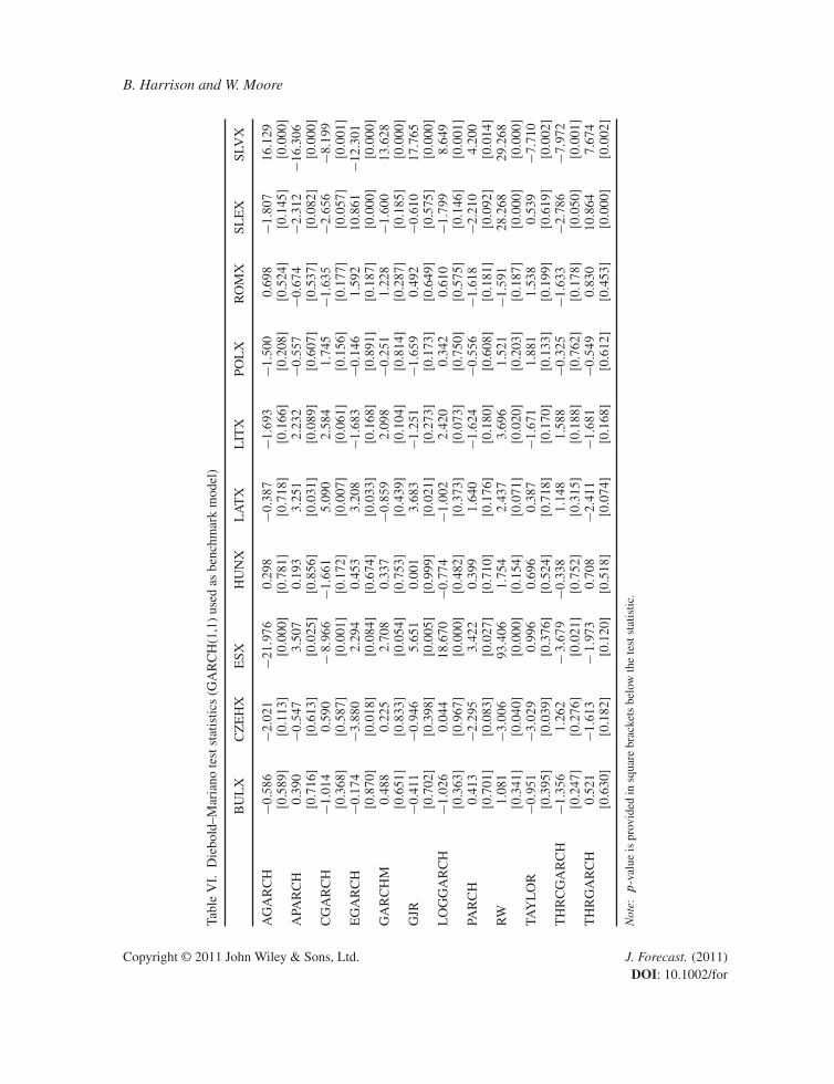
To identify whether or not the forecast errors from the more sophisticated models are statisticallydifferent from those of the relatively simple GARCH(1,1) model, the DM test statistic is calculatedfor the 1-week trading horizon. The results are provided in Table VI. In most countries, the simpleGARCH(1,1) model has expected forecast errors that are statistically different from those for morecomplex models. Indeed, in Bulgaria, Hungary, Lithuania, Poland and Romania, none of the DMstatistics for the 12 volatility forecasting models considered are statistically significant.



Tabl

eII

I.O

ut-o

f-sa

mpl

efo

reca

stin

gac

cura

cy(t

radi

ngw

eek)

One

wee

kR

elat

ive

eval

uatio

nst

atis

ticR

ank

Med

ian

rank

MSE

1M

SE2

QL

IKE

R2L

OG

MA

D1

MA

D2

MSE

1M

SE2

QL

IKE

R2L

OG

MA

D1

MA

D2

AG

AR

CH

0.68

310.

594

3.00

30.

858

0.72

00.

646

86

711

87

8A

PAR

CH

0.69

690.

628

3.94

60.

848

0.72

50.

663

1010

108

910

10C

GA

RC

H0.

6701

0.61

810

.664

0.80

40.

690

0.64

55

812

12

66

EG

AR

CH

0.64

900.

572

1.77

20.

837

0.69

70.

623

11

33

32

3G

AR

CH

0.66

320.

589

3.48

20.

841

0.70

20.

627

43

96

53

5G

AR

CH

M0.

7022

0.61

73.

117

0.85

80.

732

0.66

111

78

1210

910

GJR

0.68

840.

620

1.63

80.

854

0.74

20.

677

99

210

1211

10L

OG

GA

RC

H0.

6613

0.59

22.

333

0.83

70.

711

0.63

63

54

57

55

PAR

CH

0.64

980.

574

4.75

90.

837

0.68

50.

616

22

114

11

2TA

YL

OR

0.72

740.

683

2.93

70.

851

0.73

90.

685

1212

69

1112

12T

HR

CG

AR

CH

0.68

140.

629

14.8

890.

820

0.70

20.

653

711

132

48

8T

HR

GA

RC

H0.

6718

0.59

02.

622

0.84

50.

704

0.63

16

45

76

46



Tabl

eIV

.O

ut-o

f-sa

mpl

efo

reca

stin

gac

cura

cy(t

radi

ngm

onth

)

MSE

1M

SE2

QL

IKE

R2L

OG

MA

D1

MA

D2

MSE

1M

SE2

QL

IKE

R2L

OG

MA

D1

MA

D2

Med

ian

rank

AG

AR

CH

0.94

640.

942

1.64

80.

980

1.03

90.

988

94

612

1210

10A

PAR

CH

0.94

300.

952

1.91

30.

962

1.01

20.

962

78

108

86

8C

GA

RC

H0.

8856

0.93

63.

856

0.91

10.

941

0.91

82

212

12

22

EG

AR

CH

0.90

050.

944

1.53

00.

947

0.97

10.

928

46

44

44

4G

AR

CH

0.95

550.

962

1.79

80.

956

1.02

10.

993

1011

95

911

10G

AR

CH

M0.

9582

0.95

51.

619

0.97

71.

036

0.98

211

95

1111

810

GJR

0.89

930.

956

1.40

50.

936

0.93

80.

905

310

23

11

3L

OG

GA

RC

H2.

9121

18.6

941.

527

0.97

01.

322

2.31

513

133

1013

1313

PAR

CH

0.91

680.

941

2.12

90.

956

0.99

80.

959

53

116

55

5R

W1.

0000

1.00

01.

000

1.00

01.

000

1.00

012

121

136

1212

TAY

LO

R0.

9277

0.94

31.

763

0.95

81.

010

0.97

06

58

77

77

TH

RC

GA

RC

H0.

8851

0.93

34.

448

0.92

10.

951

0.92

41

113

23

33

TH

RG

AR

CH

0.94

390.

947

1.67

60.

970

1.02

80.

984

87

79

109

9



Tabl

eV

.O

ut-o

f-sa

mpl

efo

reca

stin

gac

cura

cy(t

radi

ngqu

arte

r)

MSE

1M

SE2

QL

IKE

R2L

OG

MA

D1

MA

D2

MSE

1M

SE2

QL

IKE

R2L

OG

MA

D1

MA

D2

Med

ian

rank

AG

AR

CH

0.90

30.

985

1.30

00.

984

0.97

40.

954

73

211

109

8A

PAR

CH

0.90

40.

998

1.57

60.

974

0.95

90.

936

88

118

76

8C

GA

RC

H0.

861

0.98

33.

062

0.92

50.

896

0.89

81

213

11

22

EG

AR

CH

0.87

90.

990

1.43

00.

974

0.94

00.

916

45

66

44

5G

AR

CH

0.91

41.

007

1.56

00.

955

0.95

00.

959

1112

103

610

10G

AR

CH

M0.

911

0.99

81.

333

0.98

30.

971

0.94

810

93

109

79

GJR

0.86

60.

999

1.35

00.

974

0.93

10.

893

310

47

31

4L

OG

GA

RC

H2.

271

14.1

751.

362

0.98

21.

177

2.00

313

135

913

1313

PAR

CH

0.88

60.

988

1.48

00.

967

0.94

90.

936

54

84

55

5R

W1.

000

1.00

01.

000

1.00

01.

000

1.00

012

111

1312

1212

TAY

LO

R0.

911

0.99

11.

440

0.98

90.

986

0.96

59

77

1211

1110

TH

RC

GA

RC

H0.

866

0.98

22.

796

0.93

40.

907

0.90

82

112

22

32

TH

RG

AR

CH

0.90

00.

991

1.52

00.

972

0.96

20.

949

66

95

88

7



Tabl

eV

I.D

iebo

ld–M

aria

note

stst

atis

tics

(GA

RC

H(1

,1)

used

asbe

nchm

ark

mod

el)

BU

LX

CZ

EH

XE

SXH

UN

XL

AT

XL

ITX

POL

XR

OM

XSL

EX

SLV

X

AG

AR

CH

�0.586

�2.021

�21.976

0.29

8�0.387

�1.693

�1.500

0.69

8�1.807

16.1

29[0

.589

][0

.113

][0

.000

][0

.781

][0

.718

][0

.166

][0

.208

][0

.524

][0

.145

][0

.000

]A

PAR

CH

0.39

0�0.547

3.50

70.

193

3.25

12.

232

�0.557

�0.674

�2.312

�16.306

[0.7

16]

[0.6

13]

[0.0

25]

[0.8

56]

[0.0

31]

[0.0

89]

[0.6

07]

[0.5

37]

[0.0

82]

[0.0

00]

CG

AR

CH

�1.014

0.59

0�8.966

�1.661

5.09

02.

584

1.74

5�1.635

�2.656

�8.199

[0.3

68]

[0.5

87]

[0.0

01]

[0.1

72]

[0.0

07]

[0.0

61]

[0.1

56]

[0.1

77]

[0.0

57]

[0.0

01]

EG

AR

CH

�0.174

�3.880

2.29

40.

453

3.20

8�1.683

�0. 146

1.59

210

.861

�12.301

[0.8

70]

[0.0

18]

[0.0

84]

[0.6

74]

[0.0

33]

[0.1

68]

[0.8

91]

[0.1

87]

[0.0

00]

[0.0

00]

GA

RC

HM

0.48

80.

225

2.70

80.

337

�0.859

2.09

8�0.251

1.22

8�1.600

13.6

28[0

.651

][0

.833

][0

.054

][0

.753

][0

.439

][0

.104

][0

.814

][0

.287

][0

.185

][0

.000

]G

JR�0.411

�0.946

5.65

10.

001

3.68

3�1.251

�1.659

0.49

2�0.610

17.7

65[0

.702

][0

.398

][0

.005

][0

.999

][0

.021

][0

.273

][0

.173

][0

.649

][0

.575

][0

.000

]L

OG

GA

RC

H�1.026

0.04

418

.670

�0.774

�1.002

2.42

00.

342

0.61

0�1.799

8.64

9[0

.363

][0

.967

][0

.000

][0

.482

][0

.373

][0

.073

][0

.750

][0

.575

][0

.146

][0

.001

]PA

RC

H0.

413

�2.295

3.42

20.

399

1.64

0�1.624

�0.556

�1.618

�2.210

4.20

0[0

.701

][0

.083

][0

.027

][0

.710

][0

.176

][0

.180

][0

.608

][0

.181

][0

.092

][0

.014

]R

W1.

081

�3.006

93.4

061.

754

2.43

73.

696

1.52

1�1.591

28.2

6829

.268

[0.3

41]

[0.0

40]

[0.0

00]

[0.1

54]

[0.0

71]

[0.0

20]

[0.2

03]

[0.1

87]

[0.0

00]

[0.0

00]

TAY

LO

R�0.951

�3.029

0.99

60.

696

0.38

7�1.671

1.88

11.

538

0.53

9�7.710

[0.3

95]

[0.0

39]

[0.3

76]

[0.5

24]

[0.7

18]

[0.1

70]

[0.1

33]

[0.1

99]

[0.6

19]

[0.0

02]

TH

RC

GA

RC

H�1.356

1.26

2�3.679

�0.338

1.14

81.

588

�0.325

�1.633

�2.786

�7.972

[0.2

47]

[0.2

76]

[0.0

21]

[0.7

52]

[0.3

15]

[0.1

88]

[0.7

62]

[0.1

78]

[0.0

50]

[0.0

01]

TH

RG

AR

CH

0.52

1�1.613

�1.973

0.70

8�2.411

�1.681

�0.549

0.83

010

.864

7.67

4[0

.630

][0

.182

][0

.120

][0

.518

][0

.074

][0

.168

][0

.612

][0

.453

][0

.000

][0

.002

]

Not

e:p

-val

ueis

prov

ided

insq

uare

brac

kets

belo

wth

ete

stst

atis

tic.



Only in the cases of the Czech Republic, Estonia, Slovenia and the Slovak Republic can volatil-ity forecasting models be identified that are statistically superior to the GARCH (1,1) model. In theCzech Republic, the EGARCH, PARCH, random walk and Taylor models had forecast errors thatare statistically smaller than those from the benchmark model. In Estonia, AGARCH, CGARCHand THRCGARCH were statistically different from zero; and for Latvia, THRGARCH was theonly model that was significant at normal levels of testing. For Slovenia and the Slovak Republic,APARCH, CGARCH and THRCGARCH were statistically different from zero in both cases. In addi-tion to these three models, the PARCH model was significant at the 10% level of testing in Slovenia,while the EGARCH and TAYLOR models had statistically significant smaller forecast errors in theSlovak Republic.

CONCLUSIONS

Overall, we have examined the forecasting performance of several well-known modelling variantswith respect to stock market volatility. The results verify the well-known result that the GARCH-type models, on average, outperform other popular, albeit naïve, forecasting models. Furthermore,we find clear evidence that incorporating some form of asymmetry over longer durations improvessubstantially the forecasting ability of volatility models. One possible explanation of this could be thepresence of volatility feedback or leverage effects in the CEE markets. Another possible explanationcould be the presence of structural changes in the CEE markets that are not taken into account andwhich the asymmetric variants are more equipped to handle. Answering which of the two possibilitiescontributes more to the forecasting performance of the asymmetric GARCH variants is an interestingarea for future research. This is not only important as an academic exercise about volatility forecasts,but, more importantly, if structural breaks explain asymmetry over longer periods, accounting forthese might provide a mechanism for increasing the robustness of forecasts in the likely event of afuture (unanticipated) break.

REFERENCES

Andersen TG, Bollerlev T, Christoffersen PF, Diebold FX. 2006a. Volatility and correlation forecasting. InHandbook of Economic Forecasting, Elliott G, Granger CWJ, Timmermann A (eds). North-Holland: Amsterdam;778–878.

Andersen TG, Bollerlev T, Christoffersen PF, Diebold FX. 2006b. Practical volatility and correlation modelling forfinancial markets risk management. In Risks of Financial Institutions, Carey M, Schultz R (eds). University ofChicago Press for NBER: Chicago, IL; 513–548.

Appiah-Kusi J, Menyah K. 2003. Return predictability in African stock markets. Review of Financial Economics12(3): 247–271.

Bernanke B, Gertler M. 1999. Monetary policy and asset price volatility. In New Challenges for Monetary Policy: ASymposium Sponsored by the Federal Reserve Bank of Kansas City. Federal Reserve Bank of Kansas City; 77–128.

Bollerslev T. 1986. Generalised autoregressive conditional heteroskedasticity. Journal of Econometrics 31:307–327.Campbell JY. 2000. Asset pricing at the millennium. NBER Working Paper No. 7589.Davis M, Polumbo M. 2001. A primer on the economics and time series econometrics of the wealth effect. Board

of Governors of the Federal Reserve System Finance and Economics Discussion Paper Series No. 2001-09,Washington, DC.

Diebold FX, Mariano RS. 1995. Comparing predictive accuracy. Journal of Business and Economic Statistics 13:253–263.

Ding Z, Granger CWJ, Engle RF. 1993. A long memory property of stock market returns and a new model. Journalof Empirical Finance 1: 83–106.

Dynan K, Maki D. 2001. Does stock market wealth matter for consumption? Board of Governors of the FederalReserve System, Finance and Economics Discussion Paper Series No. 2001-23, Washington, DC.



Engle RF. 1982. Autoregressive conditional heteroskedasticity with estimates of the variance of United Kingdominflation. Econometrica 50: 987–1007.

Engle RF, Bollerslev T. 1986. Modelling the persistence of conditional variances. Econometric Reviews 5: 1–50.Engle RF, Patton AJ. 2001. What good is a volatility model? Quantitative Finance 1: 237–245.Gilmore CG, McManus CM. 2001. Random walk and efficiency tests of central European markets, paper prepared

for presentation at the European Financial Management Association conference, Lugarno, Switzerland.Guo H. 2002. Stock market volatility: reading the meter. Monetary Trends, Federal Reserve bank of St Louis.Hall RE. 1978. Stochastic implications of the life cycle–permanent income hypothesis: theory and evidence. Journal

of Political Economy 86: 971–987.Harrison B, Moore W. 2009. Spillover effects from London and Frankfurt to Central and Eastern European stock

markets. Applied Financial Economics 19(18): 1509–1521.Harvey D, Leybourne S, Newbold P. 1997. Testing the equality of prediction mean squared errors. International

Journal of Forecasting 23: 801–824.Kash-Haroutounian M, Price S. 2001. Volatility in the transition markets of Central Europe. Applied Financial

Economics 11(1): 93–105.Kiley M. 2000. Identifying the effect of stock market wealth on consumption: pitfalls and new evidence. Federal

Reserve Bank of New York Economic Policy Review 5: 29–52.Lopez JA. 2001. Evaluation of predictive accuracy of volatility models. Journal of Forecasting 20: 87–109.Murinde V, Poshakwale S. 2002. Volatility in the emerging stock markets in Central and Eastern Europe: evidence

on Croatia, Czech Republic, Hungary, Poland, Russia and Slovakia. European Research Studies 4(3/4): 73–101.Nelson D. 1991. Conditional heteroskedasticity in asset returns: a new approach. Econometrica 59: 347–370.Poon S-H, Granger CJW. 2003. Forecasting volatility in financial markets: a review. Journal of Economic Literature

41(12): 478–539.Poshakwale S, Murinde V. 2001. Modelling volatility in East European emerging stock markets: evidence on

Hungary and Poland. Applied Financial Economics 11(4): 445 – 456.Runkle DE, Golsten LR, Jagannathan R. 1993. On the relation between the expected value and the volatility of the

nominal excess return on stocks. Journal of Finance 48: 1779–1801.Salomons R, Grootveld H. 2003. The equity risk premium: emerging vs developed markets. Emerging Markets

Review 4(2): 121–144.Stevans LK. 2004. Aggregate consumption spending, the stock market and asymmetric error correction. Quantita-

tive Finance 4(2): 191–198.Taylor S. 1986. Modelling Financial Time Series. Wiley: Chichester.Zakoïan J-M. 1994. Threshold heteroskedastic models. Journal of Economic Dynamics and Control 18(5): 931–955.

Authors’ biographies:Barry Harrison is senior lecturer at Nottingham Business School where he teaches Financial Economics onboth undergraduate and postgraduate programmes. His main research interests currently focus on capital mar-kets, especially those in Central and Eastern Europe. He has held teaching appointments at the Universities ofSheffield and Loughborough and visiting appointments at the European University at St Petersburg (Russia) andTiasNimbas School of Management in the Netherlands. His published work has appeared in various journalsincluding Economics Letters, Applied Financial Economics and Economic Issues.

Winston Moore teaches at The University of the West Indies and prior to that he was Senior Economist at theCentral Bank of Barbados. His research has focused on three major areas in economics: Industrial Economics,Tourism Economics and International Macroeconomics, He has published more than 50 articles in peer-reviewedjournals and books. His research has appeared in major journals such as the Journal of Forecasting, Journal ofPolicy Modeling, Annals of Tourism Research, Applied Economics and Contemporary Economic Policy.

Authors’ addresses:Barry Harrison, Nottingham Business School, Nottingham Trent University, Burton Street, Nottingham NG14BU, UK.

Winston Moore, Department of Economics, University of the West Indies, Cave Hill Campus, BridgetownBB11000, Barbados.


Documents

Forecasting Stock Market Volatility in Central and Eastern European Countries