FORECASTING STOCK MARKET VOLITILITY- EVIDENCE …oaji.net/articles/2017/2748-1485002113.pdf · At present there are 119 companies listed in Muscat Security Market ... Forecasting

International Journal of Commerce and Finance, Vol. 2, Issue 1, 2016, 37-53

FORECASTING STOCK MARKET VOLITILITY- EVIDENCE FROM MUSCAT SECURITY MARKET USING GARCH MODELS

M.Tamilselvan (Ph.D)

Faculty of Accounting &Finance, Ibri College of Technology – Sultanate of Oman

Shaik Mastan Vali (Ph.D)

Head Department of Business Studies,Ibri College of Technology – Sultanate of Oman

Abstract: Engle (1982) introduced the autoregressive conditionally heteroskedastic model for quantifying the conditional volatility and by Boollerslev (1986), Engle, Lilien and Robins (1987) and Glosten, Jaganathan and Runkle (1993) extended the class asymmetric model. Amongst many others, Bollerslev, Chou and Kroner (1992) or (1994) are considered to be the précis of ARCH family models. In this direction the paper forecasts the stock market volatility of four actively trading indices from Muscat security market by using daily observations of indices over the period of January 2001 to November 2015 using GARCH(1,1), EGARCH(1,1) and TGARCH (1,1) models. The study reveals the positive relationship between risk and return. The analysis exhibits that the volatility shocks are quite persistent. Further the asymmetric GARCH models find a significance evidence of asymmetry in stock returns. The study discloses that the volatility is highly persistent and there is asymmetrical relationship between return shocks and volatility adjustments and the leverage effect is found across all flour indices. Hence the investors are advised to formulate investment strategies by analyzing recent and historical news and forecast the future market movement while selecting portfolio for efficient management of financial risks to reap benefit in the stock market.

Keywords: GARCH, EGARCH, TGARCH, Stock market volatility

1. Introduction The stock and index returns are subject to both internal and external shocks that sharply raise the volatility. Stock volatility is simply defined as a conditional variance, or standard deviation of stock returns that is not directly observable. The primary function of the government, companies, day traders, short sellers and institutional investors is to understand the characteristics of the movements between return and volatility. Hence, the volatility forecasting become the central part of formulating investment strategies. It is approached with two perspectives, such as the variance is constant over a period of time and the other emphasizes that the variance is getting varied over time. There are few facts indentified in high frequency time series data such as fat tail, clustering volatility, leverage effect, long memory and co movement in volatility. Fama (1963, 1965) and Mandelbrot (1963) were the pioneer studies found the existence of fat tail in the financial time series data and reported that the kurtosis was greater than standardized fourth movement of normal distribution 3. Secondly, the data indicates the shock persistence. The high frequency financial time series data is assumed to possess the clustering volatility which large movements followed by further large movements. It could be detected through the existence of significant correlation at extended lag length in correlogram and corresponding Box-Ljung statistics. Thirdly, the negative correlation between the price movement and the volatility which is called as leverage effect. It is a significant character of the time series data. It was first suggested by Black (1976). He argued that the measured effect of stock price changes on volatility was too large to be explained solely by leverage effect. Further empirical evidence on leverage effect can be found in Nelson (1991), Gallant, Rossi and Tauchen (1992, 1993), Campel and Kyle (1993) and Engle and Ng (1993). Fourthly, the volatility is highly persistent and there is evidence of near unit root behavior in the conditional variance process. This observation led to two propositions for modeling persistence, the unit root or the long memory process. The autoregressive conditional heteroscedasticity (ARCH) and stochastic volatility (SV) use the later idea for modeling persistence. Fifthly, it is observed a big movement between different variables in financial time series across different markets. It suggests the importance of multivariate models in modelling cross correlations in different markets. These observations about volatility led many researchers to focus on the cause of these stylized facts.According to Liu and Morley (2009) the standard deviation of the returns over the future period should be forecasted accurately to enhance the asset’s performance. Volatility forecasting is an essential part in most finance decisions be it asset

Inte

rnati

on

al

Jou

rnal

of

Co

mm

erc

e a

nd

Fin

an

ce

38 M. Tamilselvan & Shaik Mastan Vali

http://ijcf.ticaret.edu.tr

allocation, derivative pricing or risk management. Hence the financial market volatility has become a central issue to the theory and practice of asset pricing, asset allocation, and risk management. This recognition has initiated an extensive research program into the distributional and dynamic properties of stock market volatility. Still, the unique model has not yet been proposed to estimate the time varying variance in the future return but several models are being used by researchers and practitioners.

2. The Notification Procedure Economic Competitive Mechanism of Oman Sultanate of Oman is one of the prominent economies in the Gulf Cooperation Council (GCC) retaining 40% of world oil reserves with 3.19 million people constituting 23.30% rural and 76.70% urban population. The world's 64th largest economy had achieved $80.57 billion and $81.79 billion gross domestic production during 2013 and 2014 with average of $16.76 billion between 1960-2014. The estimated foreign current reserve is $25 billion and debt GDP ratio is well maintained at 4% level. Such a robust economy is facing budget crisis due to sustained low oil price which dropped around 40% from the peak last year, since 31st July, 2014 when the oil price declined less than $100 per barrel, and went further down to less than $50 on 6thJanuary,2015 eventually it touched record low of $38.33 on 24th August,2015. The conservative Oman economy is generating 83% revenue from hydrocarbon sector. The nation’s budget massively depends around 79% on oil revenues and 21% on non-oil revenue. The overall estimated revenue for 2015 is 11.6 billion OMR (Oil revenue 9.16 billion OMR and non-oil revenue 2.4 billion OMR)which is 2.5 billion OMR lesser than the estimated public spending of 14.1 billion OMR. The cascade effect of oil price drop has an impact on the performance of industries in the different sectors in Oman. In these crucial circumstances, the Oman government is in the position to implement certain tough financial and investment decisions to manage the current financial turmoil. Firstly, cutting the, nation’s largest cash out flow, current expenditure (9.6 billion OMR)to the possible extent. Secondly, financing the project and infrastructure investment (3.2 billion OMR) through privatization and issuing government bonds, thirdly, enhancing the growth and performance of non-hydrocarbon industries to contribute incremental revenue during the crisis. Apart from these Oman has strong fundamental strength including the stable macro economy, the efficient infrastructure, the economic and investment legislations, the solid growth of non-oil sectors, the financial stability as represented by the safe public finances, banking system, the monetary policy and the stable local currency make the Sultanate capable of confronting these challenges with great confidence.

3. About Oman Capital Market The economic growth and job creation are considered to be the primary objectives of any nation which require a huge long term investments in the capital intensive assets such as revenue generating infrastructure, factories and equipment, new housing and commercial buildings, and research and development to expand the productive capacity. There exists a strong positive correlation between the growth of economy and capital market. Capital markets are the significant source of long term and short term capital where the firms mobilize funds from public for the existing and new projects thorough issuance of new securities such as shares, bonds, debentures and other money market instruments. The better allocation of low cost capital enhances the productivity and financial returns of the firms. Capital market regulations emphasize the firms to ensure an improved business and management models to achieve the financial performance and corporate governance. Oman capital market is an emerging market performing a vital role in pooling capital for the projects and investments. It is one of the well-known markets in the GCC region. At present there are 119 companies listed in Muscat Security Market (MSM) Shariah Index which are grouped under financial sector (36-Compnies), service sector (36-companies) and industrial sector (47-companies). The Omani companies and government raised 1.285 billion OMR in 2013 which is higher than the credits provided by commercial banks in Oman. The total value of the investors in Muscat security market is 14.1 billion OMR which is approximately equal to the total deposits of the commercial banks. Thus capital market is highly efficient mechanism to transmit funds from investors, savers, and the government companies needing capital. The capital market is designed for this purpose.

Forecasting Stock Market Volitility- Evidence From Muscat Security Market Using Garch Models 39


4. Literature Review Qamruzzaman(2015) examined a wide variety of popular volatility models for Chittagong stock return index from 04 January 2004 to14 September 2014 and found that there has been empirical evidence of volatility clustering. The study confirmed that these five models GARCH-z, EGARCH-z, IGARCH-z, GJR-GARCH-z and EGARCH-can capture the main characteristics of Chittagong stock exchange (CSE). Qiang Zhang (2015) explored the influence of the global financial crisis on the volatility spillover between the Mainland China and Hong Kong stock markets from January 04, 2002 to December 31, 2013. The results indicated that while there is no volatility spillover in the pre-crisis period, strong bi-directional volatility spillover exists in the crisis period.

Prashant Joshi (2014) used three different models: GARCH (1,1), EGARCH(1,1) and GJR-GARCH(1,1) to forecast daily volatility of Sensex of Bombay Stock Exchange of India from January 1, 2010 to July 4, 2014 and confirmed the persistence of volatility, mean reverting behavior and volatility clustering and the presence of leverage effect.

Neha Saini (2014) examined and compared the forecasting ability of Autoregressive Moving Average (ARMA) and Stochastic Volatility models applied in the context of Indian stock market using daily values of Sensex from Bombay Stock Exchange (BSE). The results of the study confirmed that the volatility forecasting capabilities of both the models.

Potharla Srikanth (2014) modeled the asymmetric nature of volatility by applying two popularly used asymmetric GARCH models i.e., GJR-GARH model and PGARCH model in. BSE-Sensex between 1st July, 1997 to 30th march, 2013. The results revealed that the presence of leverage effect in Indian stock market and it also confirmed the effect of periodic cycles on the conditional volatility in the market

Amitabh Joshi (2014) tried to analyze the volatility of BSE Small cap index using 3 years data from 1st July 2011

to 1st July 2013 suggested that ARCH and GARCH terms are significant.

Mohandass (2013) attempted to study the best fit volatility model using Bombay stock exchange daily sectoral indices for the period of January, 2001 to June, 2012. The findings concluded that the non-linear model is fit to model the volatility of the return series and recommended GARCH (1,1) model is the best one.

Naliniprava(2013) forecasted the stock market volatility of six emerging countries by using daily observations of indices over the period of January 1999 to May 2010 by using ARCH, GARCH, GARCH-M, EGARCH and TGARCH models. The study revealed that the positive relationship between stock return and risk only in Brazilian stock market. The analysis exhibits that the volatility shocks are quite persistent in all country’s stock market. Further the asymmetric GARCH models find a significant evidence of asymmetry in stock returns in all six country’s stock markets. This study confirmed the presence of leverage effect in the returns series.

Fereshteh , Hossein (2013) applied GARCH (1-1), and GARCH (2-2) to investigate the volatility using daily index from 2006 to 2010 for selected pharmaceutical group, vehicle group and oil industry respectively. The result showed volatilities feedback in pharmaceutical and oil industry. Positive effect of volatilities reign on output in pharmaceutical group, when this effect was negative in oil group. Also it was not confirmed in vehicle group.

Yung-Shi Liau 2013 studied the stock index returns from seven Asian markets to test asymmetric volatility during Asian financial crisis. The empirical results showed that both volatility components have displayed an increasing sensitivity to bad news after the crisis, especially the transitory part.

Ming Jing Yang 2012 explored the predictive power of the volatility index (VIX) in Taiwan market from December 2006 to March 2010. The results shown that the predictive power of the models is improved by 88% in explaining the future volatility of stock markets..

Rakesh Gupta 2012 aimed to forecast the volatility of stock markets belonging to the five founder members of the Association of South-East Asian Nations, referred to as the ASEAN-5 by using Asymmetric-PARCH (APARCH) models with two different distributions (Student-t and GED). The result showed that APARCH models with t-distribution usually perform better.



Praveen (2011) investigated BSE SENSEX, BSE 100, BSE 200, BSE 500, CNX NIFTY, CNX 100, CNX 200 and CNX 500 by employing ARCH/GARCH time series models to examine the volatility in the Indian financial market during 2000-14. The study concluded that extreme volatility during the crisis period has affected the volatility in the Indian financial market for a long duration.

Srinivasan1(2010) attempted to forecast the volatility (conditional variance) of the SENSEX Index returns using daily data, covering a period from 1st January 1996 to 29th January 2010. The result showed that the symmetric GARCH model do perform better in forecasting conditional variance of the SENSEX Index return rather than the asymmetric GARCH models.

Jibendu Kumar (2010) applied different methods i.e. GARCH, EGARCH, GJR- GARCH, IGARCH & ANN for calculating the volatilities of Indian stock markets using fourteen years of data of BSE Sensex & NSE Nifty. The result showed that, there is no difference in the volatilities of Sensex, & Nifty estimated under the GARCH, EGARCH, GJR GARCH, IGARCH & ANN models.

Amit Kumar (2009) investigated to forecast the volatility of Nifty and Sensex with the help from Autoregressive Conditional Heteroskedastic models (ARCH). The study found that EGARCH method emerged as the best forecasting tool available, among others.

Dima Alberg and Haim Shalit (2008) analyzed the mean return and conditional variance of Tel Aviv Stock Exchange (TASE) indicesusing various GARCH models. The results showed that the asymmetric GARCH model with fat-tailed densities improves overall estimation for measuring conditional variance. The EGARCH model using a skewed Student-t distribution is the most successful for forecasting TASE indices.

Floros, Christos (2008) examined the use of GARCH-type models for modelling volatility and explaining financial market risk using daily data from Egypt (CMA General Index) and Israel (TASE-100 index). The study found the strong evidence that daily returns can be characterized by the above models and concluded that increased risk will not necessarily lead to a rise in the returns.

Banerjee, A. and Sarkar, S. (2006), predicted the volatility using five-minute intervals daily return to model the volatility of a very popular stock market in India, called the National Stock Exchange. This result emphasized that the Indian stock market experiences volatility clustering and hence GARCH-type models predict the market volatility better than simple volatility models, like historical average, moving average etc. It is also observed that the asymmetric GARCH models provide better fit than the symmetric GARCH model, confirming the presence of leverage effect.

Kumar.S (2006) attempted to evaluate the ability of ten different statistical and econometric volatility forecasting models to the context of Indian stock and forex markets. The findings confirmed that G.-I RCH 11. I, and EW.1 L4 methods will lead to Netter volatility forecasts in the Indian stock market and G.4RCH (5, I) will achieve the same in the forex market.

Glen.R (2005) investigated the role of trading volume and improving volatility forecasts produced by ARCH and option models and combinations of models. The findings revealed an important switching role for trading volume between a volatility forecast that reflects relatively stale information (the historical ARCH estimate) and the option-implied forward-looking estimate.

Hock Guan Ng (2004) estimated the asymmetric volatility of daily returns in Standard and Poor’s 500 Composite Index and the Nikkei 225 Index in the presence of extreme observations, or significant spikes in the volatility of daily returns. The study concluded that both the GARCH(1,1) and GJR(1,1) models show superior forecasting performance to the Risk Metrics model. In choosing between the two models, however, superiority in forecasting performance depends on the data set used.

Philip (1996) studied the predictive power of GARCH model and two of its nonlinear modification to forecast weekly stock market volatility for the German stock market, Netherland, Spain, Italy and Sweden for 9 years from 1986 to 1994. The study found that the QGARCH model is the best when the estimation sample does not contain extreme observations such as the 1987 stock market crash.



Glosten, L. (1993) adopted the modified GARCH-M model, and proved that monthly conditional volatility may not be as persistent as was thought. Positive unanticipated returns appear to result in a downward revision of the conditional volatility whereas negative unanticipated returns result in an upward revision of conditional volatility.

Engle, R. and Ng, V. K. (1993), attempted to estimate news impact on volatility using daily return from Japan stock market. The result suggested that the Glosten, Jagannathan and Runkle (GJR) is the best parametric model.

Nelson (1991) analyzed the daily returns of CRSP value weighted index from 1962 to 1987 to propose a new ARCH model to overcome the three major drawbacks of GARCH model. The findings contribute a new class of ARCH models that does not suffer from the drawbacks of GARCH model allowing the same degree of simplicity and flexibility in representing conditional variance as ARIMA and related models have allowed in representing conditional mean.

Akgiray, V. (1989) presented a new evidence about the time series behavior of stock price using 6,030 daily returns from Center for Research in Security Prices (CRSP) from January 1963 to December 1986. The findings observed the second order dependence of the daily stock returns which could not be modeled with linear white noise process. Therefore study concluded that the GARCH models are superior in forecasting volatility.

Bollerslev (1986) introduced a new, more general class of processes, GARCH (Generalized Autoregressive Conditional Heteroskedastic allowing flexible lag structure. The extension of the ARCH process to the GARCH process bears much resemblance to the extension of the standard time series AR process to the general ARMA process and, permits a more parsimonious description in many situations.

Engle, R. F. (1982) introduced a new class of stochastic process called autoregressive conditional heteroscedasticity to generalize the implausible assumptions of the traditional econometric models by estimating the means and variances of inflation in the UK. The study found significant ARCH effect and substantial volatility increase during seventies.

5. Research Methodology The study has chosen four actively performing indices from Muscat security market such as MSM-30 Index, Financial Index, Service Index and Industrial Index. The required time series daily closing prices of all four indices have been collected from January 2001 to November 2015 from www.msm.com. The return is calculated as the continuously compound return using the closing price index.

)1(100*)/ln( 1 ttt PPR

Where tRis the return in the period t , tP

is the daily closing price at a particular time t ; 1tP is the closing price

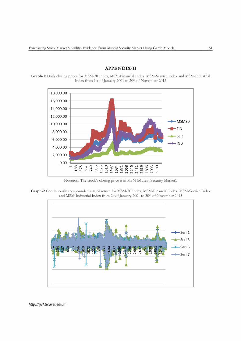
for the preceding period and ln is the natural logarithm. The graphs 1 and 2 are showing the prices and returns trend of the sample indices for the study period.

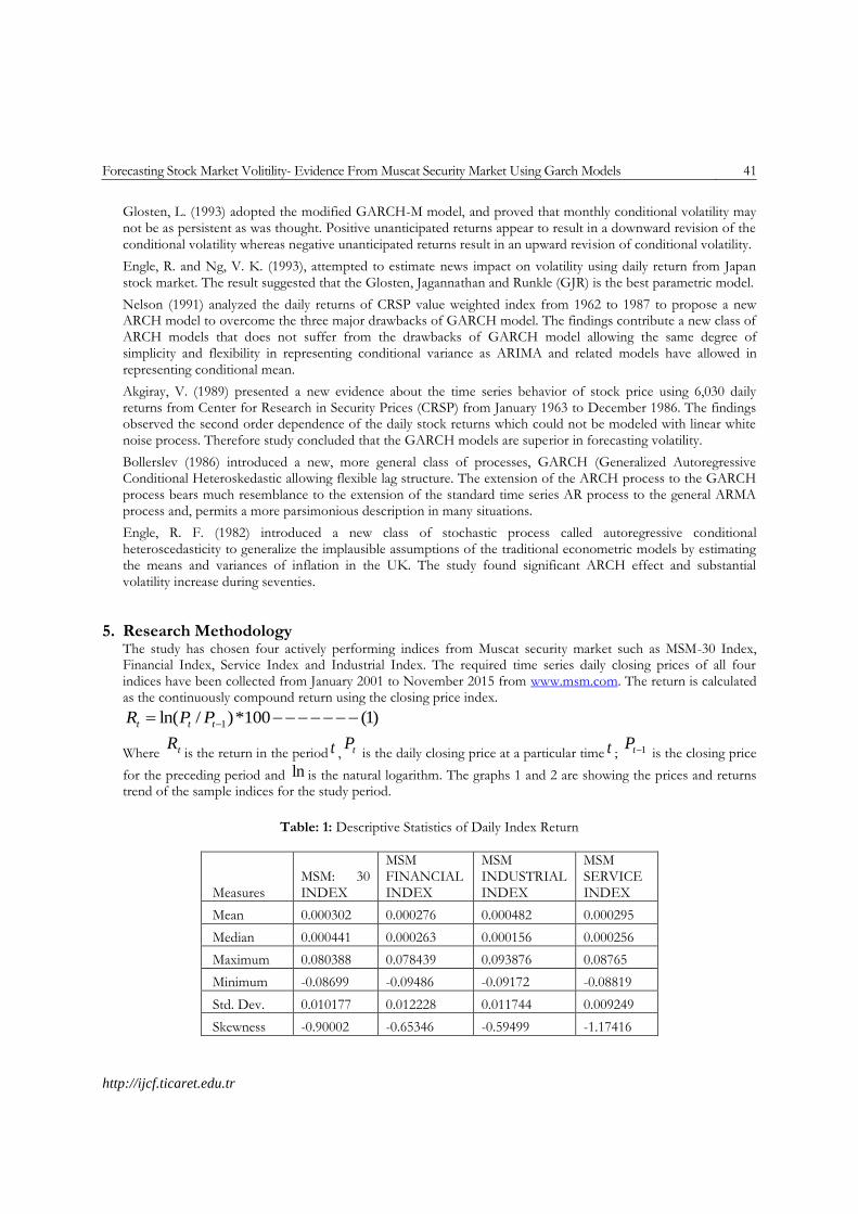
Table: 1: Descriptive Statistics of Daily Index Return

Measures MSM: 30 INDEX

MSM FINANCIAL INDEX

MSM INDUSTRIAL INDEX

MSM SERVICE INDEX

Mean 0.000302 0.000276 0.000482 0.000295

Median 0.000441 0.000263 0.000156 0.000256

Maximum 0.080388 0.078439 0.093876 0.08765

Minimum -0.08699 -0.09486 -0.09172 -0.08819

Std. Dev. 0.010177 0.012228 0.011744 0.009249

Skewness -0.90002 -0.65346 -0.59499 -1.17416

http://www.msm.com/



Kurtosis 19.22587 14.32754 15.77624 24.70162

Jarque-Bera 37323.78 18208.38 23057.63 66726.37

Probability 0 0 0 0

Source: Data Analysis

Descriptive statistics of the selected indices mean returns, standard deviations; skewness, kurtosis, and Jarque Berra test are reported in the above Table 1.The highest mean returns are given by industrial index of 0.05%with the standard deviation of 1.17%. The other three indices MSM-30, financial index and service index gained 0.03% return with the standard deviation of 1, 02%,1.22% and .92%. The residuals of the time series data for all indices are found non normality having rejected the null hypothesis in Jarque-Bera test. The time series data is required to possess certain characteristic to apply the ARCH family models. Therefore, the data is involved for detecting the presence of stationarity and clustering volatility, using unit root ADF and PP test and ARCH test. Augmented Dickey – Fuller Test (ADF) The time series data is assumed to be non-stationary. To ensure the existence of stationary relationship, the following econometric models like Augmneted Dickey Fuller (ADF) and Philps –Perron (PP) tests are employed in the study.

)2(120

tt

k

li

t t

Where, t denotes the daily price of the individual stock at time “t” and “ 1 ” is the coefficient to be estimated, k is

the number of lagged terms, t is the trend term, 2 is the estimated coefficient for the trend, 0

is the constant,

and is white noise. MacKinnon’s critical values are used in order to determine the significance of the test statistic. Phillips-Perron (PP) Test Phillips and Perron (1988) suggest an alternative (nonparametric) method of controlling of serial correlation when testing for a unit root. Phillips and Perron use nonparametric statistical methods to take care of the serial correlation in the error terms without adding lagged difference terms. Since the asymptotic distribution of the PP test is the same as the ADF test statistic. The PP method estimates the non-augmented DF test equation and modifies the t-ratio of the coefficient so that serial correlation does not affect the asymptotic distribution of test statistic. The advantage of Phillips and Perron test is that it is free from parametric errors. PP test allows the disturbances to be weakly dependent and heterogeneously distributed. The PP test is based on the following statistic.1

)3(

22/1

0

00

2/1

0

0

f

fT

ft t

Where α is the estimate, and t is the ratio of α and t is coefficient standard error and ε is the standard error

of the test regression. In addition 0yis a consistent estimate of the error variance. The remaining term 0f is

estimator of the residual spectrum at frequency zero. The present study employs the Augmented Dickey Fuller test and PP test to examine whether the time series properties are stationary or not using level series with trend and intercept. The results show that the test statistics of all four indices is higher than the critical value at 5% level. Hence the null hypotheses of ADF and PP tests are rejected and concluded that the return series data are stationary at level.

1Tripathy, Forecasting Stock Market Volatility: Evidence From Six Emerging Markets, Journal of International Business and Economy: 69-93



Table: 2: ADF and PP Tests for Unit Root

INNDICES NAME

Augmented Dickey Fuller test Philips- Perron Test

TEST STATISTICS

CRITICAL VALUE 5%

TEST STATISTICS

CRITICAL VALUE 5%

MSM 30 INDEX -44.54387 -3.411143 -44.13303 -3.411143

FINANCIAL INDEX -45.22041 -3.411143 -44.76095 -3.411143

INDUSTRIAL INDEX -44.00809 -3.411143 -44.11518 -3.411143

SERVICE INDEX -47.47459 -3.411143 -47.46145 -3.411143

Source: Data Analysis Note: Null Hypothesis is rejected at the level of 5% significance

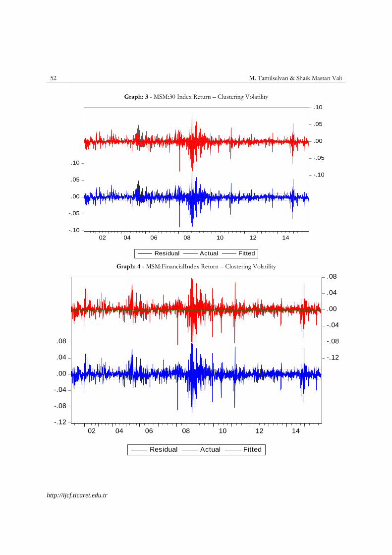
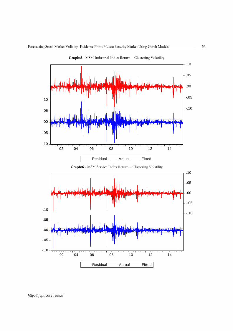
After ensuring the non-existence of unit root in time series data, it should be further investigated whether the data is found with clustering volatility and ARCH effect. The clustering volatility means Periods of low volatility tend to be followed by periods of low volatility for a prolonged period. Again, periods of high volatility is followed by periods of high volatility for a prolonged period. When clustering volatility and ARCH effect are found in the time series data, then the forecasting can be estimated using ARCH family models. In this regard, the trend of graph 3, 4, 5 and 6 shown in Appendix-II and the estimates of ARCH test prove with p-value of 0.0000 for all four indices that the sample time series index return data is suffering from ARCH and clustering volatility and reject the null hypothesis. The graph 1 and 2 are portraying the trend of price and return series of the sample indices. Hence it is determined to use the ARCH family models such as GARCH(1,1), EGARCH and TGARCH.

Table 3: Estimates of ARCH - Test

INDICES OBS*R-Squared P-Value

MSM -30 INDEX 883.3364 0.0000

FINANCIAL INDEX 677.2618 0.0000

INDUSTRIAL INDEX 825.4853 0.0000

SERVICE INDEX 1100.498 0.0000

Source: Data Analysis GARCH Model

In order to determine the nature of conditional volatility Garch model developed by Bollerslev (1986) has been used. The model can be specified as follows:

)4(1 aeRCR ttt

bhNee ttt 4),0(/ 1

)4(1

12

1cheh jtjj

ptiii

q

t

Where, tRin return equation is the stock market return in time period t and te

pure white noise error term. In

variance equation th is the conditional variance and ɷ, pq ,,,, 121 are parameters to be estimated. q is the

number of squared error term lags in the model and p is the number of past volatility lags included in the model. The

study has used the Garch (1,1) Model that assume ɷ > 0, α and β≥ 0. The stationary condition for Garch (1,1) is α +β< 1. If this condition is fulfilled, it means the conditional variance is finite. A straightforward interpretation of the

estimated coefficient in above equation is that the constant ɷ is long – term average volatility where 1 and 1 represent how the volatility is affected by current news and past information regarding volatility, respectively.



EGARCH Model

To ascertain the effect of unexpected shock on the mean return Exponential Garch or Egarch model has been used by the study as it is most popular among the asymmetric Garch models. The model is based on the log transformation of conditional variance, the conditional variance always remains positive. The model has been developed by Nelson (1991). The study used the following model specifications:

)6(1 aeRCR ttt

bhNee ttt 6),0(/ 1

)6()ln()( 1111110 chZZEZh ttttt

Here, 1tZis the standard residual. The term

)( 11 tt ZEZ measures the size effect of innovations in returns

on volatility, while 1t measures the sign effect. A negative value of 𝛿 is consistent with leverage effect, which explains that when the total value of a leveraged firm falls due to fall in price, the value of its equity becomes a smaller share of the total value. The total effect of a positive shock in return is equal to one standardized unit is (1+

𝛿), that of a negative shock of one standardizes unit is (1- 𝛿). 1 is the coefficient of autoregressive term in variance

equation. The value of 1 must be less than 1 for stationarity of the variance.

TGARCH Model

To confirm the results produced by the EGARCH model, TGARCH model has also been used in the study. This model is also named as GJR (Glosten, Jagannathan and Runkle ,1993). The specification of the TGARCH model used in the study is as follows

)7(1 aeRCR ttt

bhNee ttt 7),0(/ 1

)7(11112

12

10 chDeeh ttttt

Where, the dummy variable 1tDrepresents the bad news, a positive value of 𝛿 signify an asymmetric volatility

response. When the innovation in return 1teis positive, the total effect in the variance is 1

2te while the return

shock is negative the total effect in the variance is 12)( te

.

6. EMPIRICAL ANALYSIS

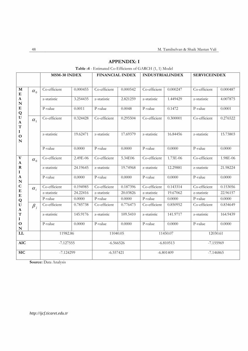
In order to verify the relationship between return and volatility of four important indices in Muscat security market GARCH family models have been applied. The results of the GARCH (1,1) model exhibits in Table:4. It presents the coefficient values of mean and variance equations for all the four indices. In the variance equation the calculated

coefficients are i0.194985, j

0.785738 (MSM: 30 – Index) i0.187396, j

0.776473 (MSM: Financial Index)

i0.143314, j

0.850952 (MSM: Industrial Index) and i0.153056, j

0.834649 (MSM: Service Index)

respectively. The sum of calculated coefficients iand j

is less than 1 for all four indices. So, the GARCH (1,1)

model is considered to be valid. In the model the value explains that irecent news is linearly related to the present

volatility of the sample indices’ return of Muscat security market. In contrast the historical volatility is measured by

jcoefficient. It is positive and higher than i

for all four indices. It implies that the recent news and past news



have an impact on the volatility of MSM: 30 index, MSM: financial index, MSM: industrial index and MSM: service index in Muscat security market in Sultanate of Oman. Since the conventional GARCH models are unable to capture the asymmetric effect of negative or positive returns on volatility, the study employed the EGARCH and TGARCH models to investigate the presence of asymmetry and leverage effect. EGARCH and TGARCH models help to explain the volatility of spot market when some degree of asymmetric is present in the price series. If the bad news has a greater impact on volatility than good news, a leverage effect exists.

Table - 5 presents the results of TGARCH (1,1) models. The coefficient of TGARCH (1,1) model is 0.787629, 0.775223, 0.855391 and 0.835031. These are all greater than zero suggesting the presence of leverage effect, i.e. the volatility to positive innovations is larger than that of negative innovations. It is also observed that in the TGARCH(1,1) model, the estimate of βi 0.147525, 0.132158, 0.125029 and 0.103017 are smaller than that of δ0.787629, 0.775223, 0.855391 and 0.835031, inferring that negative shocks do not have greater impact on conditional volatility compared to positive shocks of same magnitude.

The EGARCH (1, 1) estimates are shown in Table - 6. Asymmetry 1

coefficient of MSM: 30 Index MSM - Financial index MSM - Industrial index and MSM - Service index are 0.953738, 0.943306, 0.969600 and 0.951811. The asymmetric effect is positive and highly significant suggesting that the volatility is depending on its past behavior. So it is evident that the Muscat stock market return is not affected with negative shocks. AIC and SIC criteria used in the above all models indicating low for the regression which is quite reasonable and fit for models.

7. Conclusion:

This paper inspects the time-varying risk and return of four indices of Muscat security market by using ARCH family models i.e GARCH (1, 1), EGARCH (1, 1)and TGARCH (1,1). The symmetric GARCH (1, 1) model estimates the sum of ARCH and GARCH coefficients close to 1 specifying that the shock to the conditional variance is highly persistent in all four indices of Muscat security market. It is realized that the greater sum of coefficients directs a large positive and negative return and a long run future volatility in the return. It guides that the volatility in Muscat security market changes for a long time. Hence GARCH (1,1) process can be used in Muscat security market to predict the future behavior of market volatility.

The asymmetric TGARCH model found the leverage effect between relationship between return shocks and volatility and emphasizing negative shocks do not have greater impact on conditional volatility compared to positive shocks of same magnitude in all four indices of Muscat security market. The EGARCH (1,1) estimation of highly significant positive coefficients proves that the existence of asymmetric effect in Muscat security market. The study discloses that the volatility is highly persistent and there is asymmetrical relationship between return shocks and volatility adjustments which may cause low earnings for business and corporate.

The Oman economy is a conservative economy maintaining robust economic fundamentals such as lower inflation, currency stability, lower fiscal deficit, lower debt GDP ratio, higher percapita income and adequate foreign current reserves. The Oman capital and stock market is an infant and emerging market compared to west and few leading Asian markets, and considered to be the key competitor in the Middle East witnessing the total trade of 2,268,748,228 OMR in 2014 comprising 79.43% Omanis, 7.34% GCC nationals, 1.82% Arabs and 11.41% foreign nationals. Around 4/5 of the investors are local nationals hardly 11.41% foreign investors participate in trading. Out of 79.43% Omanis 51.36% constitutes institutions and the remaining 28.07% is individuals. Even though, the domestic fundamentals are good the persistent volatility and asymmetrical relationship are witnessed in the returns of the Muscat security market. Hence, it is the collective responsibilities of individuals, institutions and the regulators to ensure the return on investment by proper analysis and forecasting of volatility of future returns.

References

Akgiray, V. (1989), “Conditional Heteroscedasticityin Time Series of Stock Returns. Evidence and Forecasts,” Journal of Business, Vol. 62 (1),pp. 55-80.

Amit Kumar Jha(2009)Predicting the Volatility of Stock Markets and Measuring its Interaction with Macroeconomic Variables: Indian Evidence, Case Study of NIFTY and SENSEX International Journal of Sciences: Basic and Applied Research (IJSBAR) ISSN 2307-4531



Amitabh Joshi(2014)volatility in returns of bse small cap index using Garch (1,1), svim e-journal of applied management vol-ii, issue- i, april 2014, issn no-2321-2535

Bollerslev (1986) Generalized Autoregressive ConditionalHeteroskedasticity Journal of Econometrics 31 (1986) 307-327. North-Holland

Banerjee, A. and Sarkar, S. (2006), “Modeling dailyVolatility of the Indian Stock Market using intra-dayData”, Working Paper Series No. 588, Indian Instituteof Management Calcutta.

Dima Alberg and Haim Shalit (2008) Estimating stock market volatility using asymmetric GARCH models, Applied Financial Economics, 2008, 18, 1201–1208

Engle, R. F. (1982), “Autoregressive ConditionalHeteroscedasticity with Estimates of the Varianceof U.K. Inflation”, Econometrica, Vol. 50 (4),pp. 987-1008.

Engle, R. and Ng, V. K. (1993), “Measuring andTesting the Impact of News on Volatility”, Journal of Finance, Vol. 48 (5), pp. 1749-1778.

Floros, Christos (2008), Modelling volatility using GARCH models: evidence from Egypt and Israel.Middle Eastern Finance and Economics (2). pp. 31-41. ISSN 1450-2889

Fereshteh , Hossein (2013), International Journal of Scientific & Engineering Research, Volume 4, Issue 11, November-2013 1785 ISSN 2229-5518

Glosten, L. R., Jagannathan, R., and Runkle, D. E. (1993), “On the Relation between the Expected Value and the Volatility of the Nominal Excess Return on Stocks”, Journal of Finance, Vol. 48 (5), pp. 1779-1801.

Glen.R (2005)volatility forecasts, trading volume, and the Arch Versus option-implied volatility trade-off, The Journal of Financial Research • Vol. XXVIII, No. 4 • Pages 519–538 • Winter 2005

Jibendu Kumar (2010) Artificial Neural Networks – An Application To Stock Market Volatility, International Journal of Engineering Science and Technology Vol. 2(5), 2010, 1451-1460

Hock Guan Ng 2004 Recursive modelling of symmetric and asymmetric volatility in the presence of extreme observations International Journal of Forecasting 20 (2004) 115– 129

Ming Jing Yang 2012 The Forecasting Power of the Volatility Index in Emerging Markets:Evidence from the Taiwan Stock Market International Journal of Economics and Finance Vol. 4, No. 2; February 2012

Mohandass (2013)Modeling volatility of bse sectoral indices international journal of marketing, financial services & management research, issn 2277- 3622 Vol.2, no. 3, march (2013)

Nelson (1991) Conditional Heteroscedasticity in Asset Returns: A New Approach, Econometrica, Vol.59, No.2 PP 347-370

Naliniprava (2013) Forecasting Stock Market Volatility: Evidence From Six Emerging Markets,Journal Of International Business And Economy (2013) 14(2): 69-93

Neha Saini(2014) Forecasting Volatility in Indian Stock Market using State Space Models, Journal of Statistical and Econometric Methods, vol.3, no.1, 2014, 115-136 ISSN: 1792-6602 (print), 1792-6939 (online)

Philip (1996) Forecasting Stock Market Volatility Uisng (Non – Linear Garch Models,Journal of forecasting, Vol:15 pp 229-235

Praveen Kulshreshtha (2011) Volatility in the Indian Financial Market Before, During and After the Global Financial Crisis Journal of Accounting and Finance Vol. 15(3) 2015

PotharlaSrikanth(2014)Modeling Asymmetric Volatility in Indian Stock Market, Pacific Business Review International Volume 6, Issue 9, March 2014

Prashant Joshi 2014 Forecasting Volatility of Bombay Stock Exchange International journal of current research and acdemic review - ISSN: 2347-3215 Volume 2 Number 7 (July-2014) pp. 222-230

Prashant Joshi (2014) Forecasting Volatility of Bombay Stock Exchange, International journal of current research and academic review.ISSN – 2347-3215



Qamruzzaman(2015) Estimating and forecasting volatility of stock indices using asymmetric GARCH models and Student-t densities: Evidence from Chittagong Stock Exchange, International Journal of Business and Finance Management Research, ISSN 2053-1842

Qiang Zhang (2015) Global financial crisis effects on volatility spillover between Mainland China and Hong Kong stock markets Investment Management and Financial Innovations, Volume 12, Issue 1, 2015

Rakesh Gupta (2012) Forecasting volatility of the ASEAN-5 stock markets: a nonlinear approach with non-normal errors Griffith University ISSN 1836-8123.

S. S. S. Kumar (2006)Comparative Performance of Volatility Forecasting Models in Indian Markets, Decis ion. Vol. 33, :Vo.2, July - D e c embe r , 2006

Srinivasan1(2010) Forecasting Stock Market Volatility of Bse-30 Index Using Garch Models, Asia-Pacific Business Review Vol. VI, No. 3, July - September 2010.

Yung-Shi Liau& Chun-Fan You 2013The transitory and permanent components of return volatility in Asian stock markets. Investment Management and Financial Innovations, Volume 10, Issue 4, 2013

Forecasting Volatility in the Financial Market – John Night

Muscat securities market companies guide

Muscat securities market annual reports

Central Bank of Oman annual reports



APPENDIX: I

Table :4 - Estimated Co-Efficients of GARCH (1, 1) Model

MSM-30 INDEX FINANCIAL INDEX

INDUSTRIALINDEX SERVICEINDEX

M E A N E Q U A T I O N

0

Co-efficient 0.000455 Co-efficient 0.000542 Co-efficient 0.000247 Co-efficient 0.000487

z-statistic 3.254435 z-statistic 2.821259 z-statistic 1.449429 z-statistic 4.007875

P-value 0.0011 P-value 0.0048 P-value 0.1472 P-value 0.0001

1




V A R I A N C E E Q U A T I O N

0

Co-efficient 2.49E-06 Co-efficient 5.34E06 Co-efficient 1.73E-06 Co-efficient 1.98E-06



i




j




LL 11982.86 11040.05 11450.07

12030.61

AIC -7.127555 -6.566526 -6.810513 -7.155969

SIC -7.124299 -6.557421 -6.801409 -7.146865




Table: 5 - Estimated Co-Efficients of TGARCH (1, 1) Model


INDUSTRIAL INDEX

SERVICE INDEX


Co-efficient 0.000322

Co-efficient

0.000350 Co-efficient 0,000211 Co-efficient 0.000353

z-statistic 2.193508

z-statistic 1.750461 z-statistic 0,201316 z-statistic 2.638436

P-value 0.0283

P-value 0.0800 P-value 0.2296 P-value 0.0083

Co-efficient 0.326508

Co-efficient

0.298219 Co-efficient 0.302074 Co-efficient 0.286913




0 Co-efficient 2.50E-06 Co-efficient

5.53E-06 Co-efficient 1.66E-06 Co-efficient 2.00E-06



i Co-efficient 0.147525 Co-efficient




j Co-efficient 0.089226 Co-efficient




Co-efficient 0.787629 Co-efficient




LL 11991.06 11051.00 11451.50

12043.47

AIC -7.131842

-6.572449 -6.810770

-7.163031

SIC -7.120917

-6.568541 -6.799845

-7.152105




Table: 6 - Estimated Co-Efficients of EGARCH (1, 1) Model


INDUSTRIAL INDEX

SERVICE INDEX


0




1





0

Co-efficient -0.681824 Co-efficient -0.754580 Co-efficient -0.476774 Co-efficient -0.647243

z-statistic -29.22041 z-statistic -23.24402 z-statistic -19.62751 z-statistic -20.36057


1




1

Co-efficient -0.048740 Co-efficient -0.053805 Co-efficient -0.027568 Co-efficient -0.064615

z-statistic -6.530271 z-statistic -6.505015 z-statistic -4.384225 z-statistic -10.91542


1




LL 11984.95 11042.22 11444.49

12043.47

AIC -7.128204

-6.567223

-6.806602 -7.163028

SIC -7.117279

-6.556297

-6.795677 -7.152103




APPENDIX-II

Graph-1: Daily closing prices for MSM-30 Index, MSM-Financial Index, MSM-Service Index and MSM-Industrial Index from 1st of January 2001 to 30th of November 2015

Notation: The stock’s closing price is in MSM (Muscat Security Market).

Graph-2 Continuously compounded rate of return for MSM-30 Index, MSM-Financial Index, MSM-Service Index

and MSM-Industrial Index from 2ndof January 2001 to 30th of November 2015



Graph: 3 - MSM:30 Index Return – Clustering Volatility

-.10

-.05

.00

.05

.10

-.10

-.05

.00

.05

.10

02 04 06 08 10 12 14

Residual Actual Fitted

Graph: 4 - MSM:FinancialIndex Return – Clustering Volatility

-.12

-.08

-.04

.00

.04

.08

-.12

-.08

-.04

.00

.04

.08

02 04 06 08 10 12 14




Graph:5 - MSM Industrial Index Return – Clustering Volatility

-.10

-.05

.00

.05

.10

-.10

-.05

.00

.05

.10

02 04 06 08 10 12 14


Graph:6 - MSM Service Index Return – Clustering Volatility

-.10

-.05

.00

.05

.10-.10

-.05

.00

.05

.10

02 04 06 08 10 12 14


Documents

FORECASTING STOCK MARKET VOLITILITY- EVIDENCE …oaji.net/articles/2017/2748-1485002113.pdf · At present there are 119 companies listed in Muscat Security Market ... Forecasting