Embed Size (px)
Citation preview
Forecasts of Physician Supply andRequirements
April 1980
NTIS order #PB80-181670

Library of Congress Catalog Card Number 80-600063
For sale by the Superintendent of Documents, U.S. Government Printing OfficeWashington, D.C. 20402 Stock No. 052-003 -00746-1
Foreword
Undertaken at the request of the Senate Committee on Labor and Human Re-sources, this report evaluates the assumptions, methods, and results of the two currentmodels used to forecast the number and kinds of physicians the country is likely toneed and have. Congress must rely heavily on such forecasts in shaping Federal policyand programs for aiding education in the health professions and for providing healthresources and services.
This report examines the two most important physician forecasting efforts—those of the Bureau of Health Manpower of the Department of Health and HumanServices (DHHS) and those of the DHHS-chartered Graduate Medical Education Na-tional Advisory Committee. These two efforts together are generally representative ofthe kinds of techniques that are used to forecast physician and other health personnelsupplies and requirements.
The report points out that projections of physician supply and requirements de-pend on historical data to predict future events, but even recent historical data reflectpast policies, not current ones. The limits of forecasts must be fully understood if theyare to serve as effective tools in the shaping of Federal medical policy. Those limitscould be made clearer by explicitly describing the assumptions behind any forecasts,by making alternative forecasts based on different sets of assumptions, and by expand-ing the forecasting process to include policy makers as well as technicians.
This analysis was prepared by OTA staff. Drafts of the report were reviewed byan advisory panel convened for the study, by the Health Program Advisory Commit-tee, and by various individuals associated with the forecasting activities analyzed.
JOHN H. GIBBONSDirector
iiz

OTA Health Program Advisory Committee
Frederick C. Robbins, ChairmanDean, School of Medicine, Case Western Reserve University
Stuart H. AltmanDeanFlorence Heller SchoolBrandeis University
Robert M. BallSenior ScholarInstitute of MedicineNational Academy of Sciences
Lewis H. ButlerAdjunct Professor of Health PolicyHealth Policy ProgramSchool of MedicineUniversity of California, San Francisco
Kurt DeuschleProfessor of Community MedicineMount Sinai School of Medicine
Zita FearonResearch AssociateConsumer Commission on the Accreditation
of Health Services, Inc.
Rashi FeinProfessor of the Economics of MedicineCenter for Community Health and
Medical CareHarvard Medical School
Melvin A. GlasserDirectorSocial Security DepartmentUnited Auto Workers
Patricia KingProfessorGeorgetown Law Center
Sidney S. LeeAssociate DeanCommunity MedicineMcGill University
Mark LepperVice President for ]nter-institutional AffairsRush-Presbyterian—St. Luke's Medical
Center
C. Frederick MostellerProfessor and ChairmanDepartment of BiostatisticsHarvard University
Beverlee MyersDirectorDepartment of Health ServicesState of California
Mitchell RabkinGeneral DirectorBeth Israel HospitalBoston, Mass.
Kerr L. WhiteDeputy Director of Health SciencesRockefeller Foundation
Forecasts of Physician Supply and Requirements
OTA Health Program Staff
Joyce C. Lashof, Assistant Director-, OTAHealth and Life Sciences Division
H. David Banta, Health Program Manager
Lawrence Mike, Project Director
Pamela Doty, Congressional/ Fellow
Nancy Kenney, Administration
OTA Publishing Staff
John C. Holmes, Publislzing Officer
Kathie S. Boss Debra M. Datcher Joanne Heming
Advisory Panel Members
E. Harvey Estes, Jr., ChairmanChairman, Department of Community and Family Medicine
Duke University School of Medicine
E. B. CampbellExecutive Vice PresidentLane College
Jack HadleyThe Urban Institute
John HatchSchool for Biomedical EducationCity College of New York
Lauren LeRoyHealth Policy ProgramSchool of MedicineUniversity of California, San Francisco
Charles LewisDepartment of MedicineSchool of MedicineUniversity of California, Los Angeles
Ted PhillipsAssociate Dean for Academic AffairsSchool of MedicineUnitiersity of Washington
Jane RecordHealth Services Research CenterKaiser Foundation
Alvin TarlovDepartment of MedicineSchool of MedicineUniversity of Chicago
John WennbergDepartment of Community MedicineDartmouth College

List of Acronyms
AMA — American Medical AssociationAOA — American Osteopathic AssociationBCHS — Bureau of Community Health ServicesBHM — Bureau of Health ManpowerBLS — Bureau of Labor StatisticsCMG — Canadian medical graduateCPI — Consumer Price IndexDHHS — Department of Health and Human ServicesDO – doctor of osteopathyFMG — foreign medical graduateFTE — full-time equivalentGMENAC — Graduate Medical Education National Advisory CommitteeGNP — gross national productGP — general practitionerHIS — Health Interview SurveyHMOS — health maintenance organizationsHMSA — Health Manpower Shortage AreaHSA — Health Service AreaMD — doctor of medicineMUA — Medically Underserved AreaNHI – national health insuranceNHSC — National Health Service Corps
vi
—
Contents
ChapterI. SUMMARY AND CONCLUSIONS
Introduction. . . . . . . . . . . . . . . . . . .Current Activities . . . . . . . . . . . . . .Findings and Conclusions. . . . . . . . .
supply . . . . . . . . . . . . . . . . . . .Requirements . . . . . . . . . . . . . .
2. SUPPLY . . . . . . . . . . . . . . . . . . . . . .
Aggregate Supply. . . . . . . . . . . . . . .Specialty Supply . . . . . . . . . . . . . . .Locational Distribution . . . . . . . . . .Summary. . . . . . . . . . . . . . . . . . . . .
3. REQUIREMENTS . . . . . . . . . . . . . .
Introduction. . . . . . . . . . . . . . . . . . .EconomicModels. . . . . . . . . . . . . . .
. . . . . . . . . . . .
. . . . . . . . . . . .
. . . . . . . . . . . .
. . . . . . . . . . . .
. . . . . . . . . . . .
. . . . . . . . . . . .
. . . . . . . . . . . .
. . . . . . . . . . . .
. . . . . . . . . . . .
. . . . . . . . . . . .
. . . . . . . . . . . .
. . . . . . . . . . . .
. . . . . . . . . . . .
. . . . . . . . . . . .The Bureau ofLabor Statistics Model . . . . . . . .Bureau ofHealthManpower ModeI . . . . . . . . .
TheFramework. . . . . . . . . . . . . . . . . . . . .The Baseline Configuration . . . . . . . . . . . .Contingency Modeling . . . . . . . . . . . . . . .Productivity . . . . . . . . . . . . . . . . . . . . . . .
The Graduate Medical Education National AdvisoryComparison oftheBHMand GMENACModels . . .Productivity. . . . . . . . . . . . . . . . . . . . . . . . . . . . . . .Locational Requirements . . . . . . . . . . . . . . . . . . . . .
BIBLIOGRAPHY. . . . . . . . . . . . . . . . . . . . . . . . . . . . . . .
List of Tables
. . . . . . . . . . . . . . . . . .
. . . . . . . . . . . . . . . . . .
. . . . . . . . . . . . . . . . . .
. . . . . . . . . . . . . . . . . .
. . . . . . . . . . . . . . . . . .
. . . . . . . . . . . . . . . . . .
. . . . . . . . . . . . . . . . . .
. . . . . . . . . . . . . . . . . .
. . . . . . . . . . . . . . . . . .
. . . . . . . . . . . . . . . . . .
. . . . . . . . . . . . . . . . . .
. . . . . . . . . . . . . . . . . .
. . . . . . . . . . . . . . . . . .
. . . . . . . . . . . . . . . . . .
. . . . . . . . . . . . . . . . . .
. . . . . . . . . . . . . . . . . .
. . . . . . . . . . . . . . . . . .
. . . . . . . . . . . . . . . . . .
. . . . . . . . . . . . . . . . . .
. . . . . . . . . . . . . . . . . .Committee Model . . .. . . . . . . . . . . . . . . . . .. . . . . . . . . . . . . . . . . .. . . . . . . . . . . . . . . . . .
. . . . . . . . . . . . . . . . . .
Table No.1. Derivation of Male and Female MD Retirement Rates and Death Rates by 5-YearAge
Cohort . . . . . . . . . . . . . . . . . . . . . . . . . . . . . . . . . . . . . . . . . . . . . . . . . . . . . . . . . . . .2. MD First-Year Enrollment Projections Using 1977 First-Year Enrollment as Base,
to 1987 ., . . . . . . . . . . . . . . . . . . . . . . . . . . . . . . . . . . . . . . . . . . . . . . . . . . . . . . . . . .3. DO First-Year Enrollment Projections Using 1976 First-Year Enrollment as Base,
to 1987 . . . . . . . . . . . . . . . . . . . . . . . . . . . . . . . . . . . . . . . . . . . . . . . . . . . . . . . . . . . .4. First-Year Enrollments in Medical and Osteopathic Schools Projected Under the Basic
Assumption; 1978-79 Through 1987-88. . . . . . . . . . . . . . . . . . . . . . . . . . . . . . . . . . . .5. U.S.-Trained Physicians, Graduates; Projected 1978-79 Through 1989-90. . . . . . . . . .6. U.S,-Trained Physicians, Graduates; Projected for 1980 and 1990. . . . . . . . . . . . . . . .7. Supply of Active Foreign-Trained Physicians, Using Basic Methodology,
Projected 1975-9(1. . . . . . . . . . . . . . . . . . . . . . . . . . . . . . . . . . . . . . . . . . . . . . . . . . . .8. Basic, High, and Low Projections of the FMG Active Supply . . . . . . . . . . . . . . . . . . .
Page
3
34557
15
15233038
45
454747495053596162727780
85
Page
16
17
17
181818
2020

Contents—continued
Table No. Page
9. Supply of Active Physicians by Country of Medical Education Using BasicMethodology: 1974 and Projected 1975-90 . . . . . . . . . . . . . . . . . . . . . . . . . . . . . . . . . 22
10. Supply of Active Physicians by Country of Medical Education Using BasicMethodology: Actual 1974, 1975; Projected 1980-90 . . . . . . . . . . . . . . . . . . . . . . . . . . 22
11. Data Sources on Physician Specialty Supply. . . . . . . . . . . . . . . . . . . . . . . . . . . . . . . . 2412. Internship and Residency Data Sources. . . . . . . . . . . . . . . . . . . . . . . . . . . . . . . . . . . . 2513. First-Year Residency Distribution With Subspecialty Adjustment: Sept. 1, 1974 . . . . . 2814, Percent Distribution of U. S./CMG First-Year Residency Projections Using Simple
Linear Regressions , . . . . . . . . . . . . . . . . . . . . . . . . . . . . . . . . . . . . . . . . ., . . . . . . . . 3015. Percent Distribution of FMG First-Year Residency Projections Using Simple Linear
Regressions ..........,..,........,.. . . . . . . . . . . . . . . . . . . . . . . . . . . . . . . . . 3116. Active Physicians, by Major Specialty Group: Actual 1974; Projected 1980-9(3 . . . . . . 3217. Supply of Active Physicians, by Specialty :Actual 1974; Projected 1980-90). . . . . . . . . 3318. Patient Care MDs by Selected Specialties and for High and Low States, 1976 . . . . . . . 3419. Non-Federal Physicians Providing Patient Care in Metropolitan and Nonmetropolitan
Areas, 1963-75 . . . . . . . . . . . . . . . . . . . . . . . . . . . . . . . . . . . . . . . . . . . . . . . . . . . . . . 3420. New Physicians Entering Practice, 1973 to 1987 . . . . . . . . . . . . . . . . . . . . . . . . . . . . . 3621. Percent of New Physicians Expected To Enter Primary Care ...,.... . . . . . . . . . . . . 3722. Projected County Classes of Newly Practicing Physicians. . . . . . . . . . . . . . . . . . . . . . 3723. Usual Source of Care for Urban Underserved Areas . . . . . . . . . . . . . . . . . . . . . . . . . . 3824. Estimated Principal-Provider Patient Loads of General Practitioners, Family
Practitioners, and General Internists. . . . . . . . . . . . . . . . . . . . . . . . . . . . . . . . . . . . . . 4125. Comparisons of Supply With Requirements Using Different Models . . . . . . . . . . . . . . 4626. 1960’s Projections of Physician Requirements in 1975 . . . . . . . . . . . . . . . . . . . . . . . . . 4727. Bureau of Labor Statistics Projections of Physician Supply and Requirements, 1985. . 4828. Population Matrix Used in the BHM Model . . . . . . . . . . . . . . . . . . . . . . . . . . . . . . . . 5129. Health Care Categories Used in the BHM Model . . . . . . . . . . . . . . . . . . . . . . . . . . . . . 5130. Projected Shifts in Age and Income Distribution, 1970-90 . . . . . . . . . . . . . . . . . . . . . . 5231. Projected Utilization Growth Factors, 1975-90 . . . . . . . . . . . . . . . . . . . . . . . . . . . . . . 5332. Prevalence of Selected Chronic Conditions Reported in Health [nterviews,
by Family Income . . . . . . . . . . . . . . . . . . . . . . . . . . . . . . . . . . , . . . . . . . . . . . . . . . . . 5433. Number of Disability Days per Person per Year by Family Income, 1973. . . . . . . . . . . 5434. Number of Physician Visits per Year by Poor and Not Poor Status and for Whites
and Others, 1964 and 1973 . . . . . . . . . . . , . . , . . . . . . . . . . . . . . . . . . . . . . . . . . . . . 5535. Number of Discharges From and Average Length of Stay in Short-Stay Hospitals,
by Income Status and Color, 1964and 1973 . . . . . . . . . . . . . . . . . . . . . . . . . . . . . . . 5536. Estimated Growth in Per Capita Utilization, Four Forms of Health Care . . . . . . . . . . . 5637. Increase in Demand From Population and Per Capita Utilization Changes,
1975 to 1990, BHM Model . . . . . . . . . . . . . . . . . . . . . . . . . . . . . . . . . . . . . . . . . . . . . 5638. Dependence of Trend Projections on Alternative Starting Dates in the Baseline Data . 6439. Comparison of Linear Versus Logarithmic Extrapolation of Utilization Data. . . . . . . . 6540. Allocation of Physicians by Type and Setting of Care for the 1975 Base Year,
BHM Model . . . . . . . . . . . . . . . . . . . . . . . . . . . . . . . . . . . . . . . . . . . . . . . . . . . . . . . . 6641. Illustrative Computation of Manpower Requirements. . . . . . . . . . . . . . . . . . . . . . . . . 6742. Specialty Areas and Subspecialties for Which Requirements Estimates Are Being
Planned or Considered by GMENAC . . . . . . . . . . . . . . . . . . . . . . . . . . . . . . . . . . . . . 6843. The Average Practice Profile of General Surgeons. . . . . . . . . . . . . . . . . . . . . . . . . . . . 7144. Proportion of Persons Whose Experience With Physician Visits Is Beyond the
Critical Threshold . . . . . . . . . . . . . . . . . . . . . . . . . . . . . . . . . . . . . . . . . . . . . . . . . . . . 7245. Percent of Ethnic Groups Dissatisfied With Aspects of the Medical Care System . . , . . 7246. Regional Differences in Certain Health-Care Statistics, United States, 1969-70 . . . . . . 7947. Shortage, Adequate, and Surplus Levels of Primary Care Physicians . . . . . . . . . . . . . 8048. Need for Primary Care Physicians and Psychiatrists in 1990 .., . . . . . . . . . . . . . . . . . 81
Contents—continued
Table No.
49. Criteria for Unmet Need Calculation by Area . . . . . . . . . . . . . . . . . . . . . . . . . . . . . . .50. Physician Encounters per Physician and Physician Encounters per Physician Hour by
Selected Cohorts, National Health Service Corps, 1976. . . . . . . . . . . . . . . . . . . . . . . .
List of Figures
Figure No.1.2.
3.4.5.
6.7.8.9,
10,11,
12,13.
14%
15,16,17,
Diagram of Projection of Supply of Active Physicians Through 1990 . . . . . . . . . . . . .Trend Data on Number of First-Year Residents: Total, Primary, Nonprimary CareSpecialties; 1960, 1968, 1974, and 1976 ........, . . . . . . . . . . . . . . . . . . . . . . . . . . .Trend in Number of First-Year Allopathic Residents in Four Selected Specialties . . . . .Projection of Active Physicians by Specialty. . . . . . . . . . . . . . . . . . . . . . . . . . . . . . . .Frequency Distribution of Physician Availability Indexes—Primary Care Physiciansand Surgeons for the 204 HSAs. . . . . . . . . . . . . . . . . , . . . . . . . . . . . . . . . . . . . . . . . .Per Capita Utilization of Physician office Services, 1966-76 . . . . . . . . . . . . . . . . . . . .Per Capita Utilization of Short-Term Hospital Services, 1966-76 . . . . . . . . . . . . . . . . .Per Capita Utilization of Dental office Services, 1966-76 . . . . . . . . . . . . . . . . . . . . . .Per Capita Utilization of Community Pharmacy Services, 1966-76 . . . . . . . . . . . . . . .Non-Price-Related Per Capita Utilization Trends, Physician Office Services, 1966-76.Non-Price-Related Per Capita Utilization Trends, Short-Term Hospital Services,1966 -76. . . . . . . . . . . . . . . . . . . . . . . . . . . . . . . . . . . . . . . . . . . . . . . . . . . . . . . . . . . .Non-Price-Related Per Capita Utilization Trendsr Dental Office Services, 1968-76 . . .Non-Price-Related Per Capita Utilization Trends, Community Pharmacy Services,1966 -76. . . . . . . . . . . . . . . . . . . . . . . . . . . . . . . . . . . . . . . . . . . . . . . . . . . . . . . . . . . .Illustrative Procedure for Arriving at Adjusted Needs Estimates . . . . . . . . . . . . . . . . .GMENAC Model for Estimating Physician Requirements . . . . . . . . . . . . . . . . . . . . .Consumer Satisfaction With Physician Services . . . . . . . . . . . . . . . . . . . . . . . . . . . . .Consumer Satisfaction With Physician Services, by Nature of the Experience . . . . . . .
Page
82
84
Page21
262629
355758596061
6263
6468697374
ix

1.
Summary
1.
Summary
INTRODUCTION
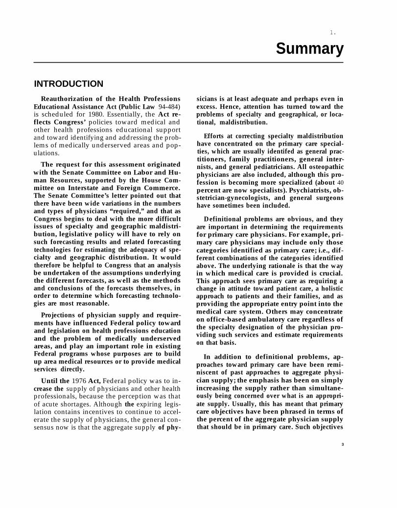
Reauthorization of the Health ProfessionsEducational Assistance Act (Public Law 94-484)is scheduled for 1980. Essentially, the Act re-flects Congress’ policies toward medical andother health professions educational supportand toward identifying and addressing the prob-lems of medically underserved areas and pop-ulations.
The request for this assessment originatedwith the Senate Committee on Labor and Hu-man Resources, supported by the House Com-mittee on Interstate and Foreign Commerce.The Senate Committee’s letter pointed out thatthere have been wide variations in the numbersand types of physicians “required,” and that asCongress begins to deal with the more difficultissues of specialty and geographic maldistri-bution, legislative policy will have to rely onsuch forecasting results and related forecastingtechnologies for estimating the adequacy of spe-cialty and geographic distribution. It wouldtherefore be helpful to Congress that an analysisbe undertaken of the assumptions underlyingthe different forecasts, as well as the methodsand conclusions of the forecasts themselves, inorder to determine which forecasting technolo-gies are most reasonable.
Projections of physician supply and require-ments have influenced Federal policy towardand legislation on health professions educationand the problem of medically underservedareas, and play an important role in existingFederal programs whose purposes are to buildup area medical resources or to provide medicalservices directly.
Until the 1976 Act, Federal policy was to in-crease the supply of physicians and other healthprofessionals, because the perception was thatof acute shortages. Although the expiring legis-lation contains incentives to continue to accel-erate the supply of physicians, the general con-sensus now is that the aggregate supply of phy-
sicians is at least adequate and perhaps even inexcess. Hence, attention has turned toward theproblems of specialty and geographical, or loca-tional, maldistribution.
Efforts at correcting specialty maldistributionhave concentrated on the primary care special-ties, which are usually identifed as general prac-titioners, family practitioners, general inter-nists, and general pediatricians. All osteopathicphysicians are also included, although this pro-fession is becoming more specialized (about 40percent are now specialists). Psychiatrists, ob-stetrician-gynecologists, and general surgeonshave sometimes been included.
Definitional problems are obvious, and theyare important in determining the requirementsfor primary care physicians. For example, pri-mary care physicians may include only thosecategories identified as primary care; i.e., dif-ferent combinations of the categories identifiedabove. The underlying rationale is that the wayin which medical care is provided is crucial.This approach sees primary care as requiring achange in attitude toward patient care, a holisticapproach to patients and their families, and asproviding the appropriate entry point into themedical care system. Others may concentrateon office-based ambulatory care regardless ofthe specialty designation of the physician pro-viding such services and estimate requirementson that basis.
In addition to definitional problems, ap-proaches toward primary care have been remi-niscent of past approaches to aggregate physi-cian supply; the emphasis has been on simplyincreasing the supply rather than simultane-ously being concerned over what is an appropri-ate supply. Usually, this has meant that primarycare objectives have been phrased in terms ofthe percent of the aggregate physician supplythat should be in primary care. Such objectives
3
4 . Forecasts of Physician Supply and Requirements
would be inappropriate if aggregate supply wereexcessive.
Geographical or locational maldistribution isgenerally a problem where health personnel andservices are found inadequate, by some definedstandard, to meet the health needs of the popu-lation of the identified communities, areas, orinstitutional settings. Locational maldistribu-tion is by definition a relative concept, wheresome of our people are determined to be at a dis-advantage relative to the rest of the UnitedStates. Once these are identified, then the gapbetween health personnel and services and thatpopulation’s needs for them is quantified to de-termine: 1) how many personnel are needed tobridge the gap, and 2) of the identified deficien-cy, how much of it will be addressed through aspecific program.
Quantifying locational maldistribution servestwo purposes. First, it is used as part of the eligi-bility criteria for the Health Manpower Short-age Area (HMSA) designation for: 1) National
CURRENT ACTIVITIES
Under the Health Professions EducationalAssistance Act of 1976, the Department ofHealth and Human Services (DHHS) is requiredto provide annual reports to the President andCongress on the status of health personnel in theUnited States. Estimating the present and futuresupply of and requirements for physicians andother health professions is the responsibility ofthe Health Resources Administration throughits Manpower Analysis Branch of the Bureau ofHealth Manpower (BHM). DHHS has producedits first report (dated August 1978 and reprintedin March 1979) and is in the final stages of re-view for its next report.
In addition, DHHS chartered a GraduateMedical Education National Advisory Commit-tee (GMENAC) on April 20, 1976, to make rec-ommendations in 3 years to the Secretary on thepresent and future supply of and requirementsfor physicians, their specialty and geographicdistribution, and methods for financing gradu-
Health Service Corps (NHSC) sites; 2) designa-tion as service areas in which students who bor-row money under health professions studentloan programs can practice in lieu of repayingthe loans in money; 3) grants for various healthmanpower training programs; 4) eligibility orpreference for grant funds for several Bureau ofCommunity Health Services programs, such asthe urban and rural health initiatives; and5) certification of rural health clinics for nursepractitioner’s and physicians’ assistant’s servicesreimbursement through Medicare and Medi-caid.
Second, these methods to quantify locationalmaldistribution are used to plan for the futuresize of NHSC. That is, given the estimated uni-verse of existing and future HMSAS, plans mustbe made for determining how many of thosemedical manpower shortage areas will bestaffed by NHSC physicians. Currently, the ma-jor source for those future NHSC positions arestudents who will be obligatedchange for scholarship support.
to NHSC in ex-
ate medical education. Its most immediate im-pact will come from its recommendations onhow graduate medical education (residency pro-grams) should (could) be changed to meet thesestated goals. GMENAC was given a l-year re-quested extension of its charter to April 20,1980, at which time its final report must be sub-mitted. An interim report was published inApril 1979.
Finally, the Bureau of Labor Statistics of theU.S. Department of Labor includes physiciansand other health occupations in its projectionsof occupational requirements and trainingneeds. These projections relate manpower toprojected economic demand (expenditures) asprovided by the Bureau’s model of the futureeconomy, which projects the future gross na-tional product (GNP) and its components—consumer expenditures, business investment,governmental expenditures, and net exports; in-dustrial output and productivity; the labor
Ch. 1—Summary Ž 5
force; average weeklyployment for detailedcupations.
hours of work; and em-industry groups and oc-
The Bureau of Labor Statistics considers theBHM’s modeling efforts to be a more sophis-ticated effort than its own, and in its forthcom-ing revision of its estimates, will adopt the mid-point of the range of projections from the BHM
FINDINGS AND CONCLUSIONS
supply
Forecasts of the future supply of physiciansconsist of:
. current Supply, adjusted for attrition fromdeaths and retirements, and
. additions to supply from:—graduates of U.S. medical and osteo-
pathic schools and—immigration of physicians educated in
other countries plus U.S. citizens edu-cated in foreign medical schools.
The supply of active physicians is projected tobe approximately 450,000 in 1980, 525,000 in1985, and 600,000 in 1990. Compared to a 1975supply of 378,000, the net increase will average75,000 every 5 years.
BHM estimates of additions to supply fromgraduates of U.S. medical and osteopathicschools take first-year enrollment projections,adjusted for attrition, to arrive at the number ofgraduates per year. Estimates of first-year en-rollments are based on trends in: 1) Federalcavitation support, 2) Federal constructiongrants activity, 3) new schools already planned,and 4) potential State and local support of newschools.
Estimates of additions to supply from immi-gration of physicians educated in other coun-tries are currently based on the presumed im-pact of the Health Professions Educational As-sistance Act of 1976, which was designed tosharply curtail the immigration of physiciansinto the United States.
model for its physician demand projections.Thus, there are essentially two major effortscurrently underway, which will have immediateimpacts on Federal health manpower policy; thesustained modeling activities of BHM and thenearly completed deliberations of DHHS’SGMENAC. These two activities also illustratewell the different approaches through whichphysician supply and requirements projectionscan be made.
GMENAC’S approach to estimating supply(not yet completed) uses a different way of dis-aggregating the U.S. medical school graduatesource. They will project graduates for eachschool, based on information provided by theAssociation of American Medical Colleges.
Although predictions of the future supplyhave been consistent in the aggregate over thepast 5 years, the additions—domestic and for-eign graduates—have changed considerably.Current projections may overestimate the num-ber of future domestic graduates because of theassumption of full cavitation funding. In con-trast, the addition to supply from foreign med-ical graduates, projected to be 1,000 to 2,000 inthe 1980’s, could be unrealistically low. U.S.students studying abroad (currently under studyby the General Accounting Office) may not beadequately accounted for and could double the1,000 to 2,000 additions per year from foreignmedical schools in the 1980’s.
The net effect of overestimating domesticsources and underestimating foreign sourcescould “wash” each other out.
Supply projections leave the impression that600,000 physicians in 1990 is a fixed number.But the assumptions currently in use explicitlyrecognize the influence of policy on supply. Esti-mates based on different sets of assumptionscould provide better indications of the variabili-ty of the projected supply and of the influence ofdeliberate policy decisions on the ultimate num-bers.
— . . — —.-—— . -- .—. .— -. —— —. — . — —
6 . Forecasts of Physician Supply and Requirements
For foreign graduates, the presumed full im-pact of Public Law 94-484 is deliberately fac-tored into the model. For domestic sources, fullcavitation and continued development of newmedical schools in the 1980’s are also assumed.The latter also reflects a presumed full impact ofexisting Federal law, but past experience andcurrent consensus would deny the real possibili-ty of ever gaining authorized cavitation levels,although private medical schools continue to bedeveloped. And the impact of Public Law94-484 on dampening foreign medical graduatesources may be circumvented by the increasingnumber of U.S. citizens studying medicineabroad and eventually returning to the UnitedStates to practice.
The specialty distribution of the projectedsupply is estimated by taking the number of ac-tive practitioners by (self-designated) specialty,adjusted for death and retirement, and distribut-ing graduates among the specialties throughprojections of first-year residency trends.
Trends in first-year residency positions areused to predict future specialty distributionbecause of lack of data on final-year residencypositions. However, first-year residency posi-tions are often used for general clinical ex-perience prior to concentration in a particularsubspecialty or in another specialty and there-fore do not necessarily represent final specialtychoices; i.e., first-year residency counts areduplicative for particular specialties in that aproportion move on to subspecialization or toanother specialty altogether. BHM’s currentprojections assume that the first-year residencydistribution trends for 1968, 1970-74, and 1976,also apply through 1980-81. After 1980-81, theresidency distribution is held constant for thestatistical reason that the base years chosen toestablish the trend cover 6 years, so BHM haschosen not to extend the extrapolation beyond 6years. Downward adjustments are made tominimize double-counting; the greatest adjust-ments occur in general surgery (62 percent) andinternal medicine (32 percent).
As a percent of the total projected supply,physicians in general practice, family practice,internal medicine, and pediatrics (those usuallycounted as primary care specialties) are pro-
jected to comprise 39 percent in 1980,41 percentin 1985, and 42 percent in 1990. The largest spe-cialty among these, as well as among all the spe-cialties, will be internal medicine, which willhave more than twice “as many physicians thanany one of the other specialties.
The locational distribution of the projectedsupply, by specialty, is estimated by similarmethods as for aggregate and specialty supply;i.e., current supply plus additions. These loca-tional projections can be disaggregate in a vari-ety of ways; e.g., by geographic criteria such asby States, counties, Census-Defined State Eco-nomic Areas, or Health Service Areas, or byspecial populations such as institutional care(mental hospitals, prisons), the indigent, andNative Americans.
Locational projections are used to identifythose locations with the least number of physi-cians for programs which intend to place physi-cians (e.g., NHSC) or for which shortage des-ignation is necessary to qualify for Governmentfunds.
The process of designating and staffingHMSAS presently includes estimating the futuresupply of physicians for: 1) rural counties; 2) ur-ban areas; 3) Federal, State, and local prisons;4) State mental hospitals and community mentalhealth centers; and S) the Indian Health Service.
Projections of specialty and locational supplydepend on the standard method of relying onhistorical data to predict future events, and inparticular, on most recent experience to predictthe most immediate future. This can be seen inthe use of mid- to late 1960’s to mid-1970’s datato predict 1980-90 patterns. Aside from the in-evitable finding of “inadequate data” which, forone of the most important marker specialties(internal medicine), contains an error factor ofat least 32 and perhaps as high as 62 percent inthe first-year residency count, the use of his-torical data has two other limitations in theseprojections of specialty and locational distribu-tion. The late 1960’s and 1970’s have witnessed:1) Medicare and Medicaid and greater third-party private insurance coverage, 2) unprece-dented increases in medical school enrollmentsand a large influx of foreign medical graduates,
—
Ch. 1.–Summary ● 7
and 3) major changes in graduate medical edu-cation, including abolition of the free-standinginternship and its selective replacement by thefirst year of some residency programs. Second,legislation in this area has purposely tried to af-fect physician specialty and location choices,and, given the lag time between physician edu-cation and eventual practice, late 1960’s andearly to mid-1970’s data reflect past policies,current ones.
Requirements
Estimates of the numbers of physiciansquired in the future are derived by dividing
not
re-the
amount of services that it is anticipated physi-cians will or should provide a given populationin a given year, by physician productivity. Esti-mates of a population’s economic demand forservices measure the capacity of the populationto use physician services and are not limited tophysician care that is essential to the patient’shealth. In general, physician productivity is as-sumed to remain constant. Thus, the differencebetween forecasting models is essentially one ofdifferences in the estimates of use.
Although productivity is generally assumedconstant, the particular measure chosen willdirectly influence the estimates of physician re-quirements. For example, GMENAC’S work-book for estimating general surgeon require-ments lists alternative estimates of averageweekly office visits that could be used as pro-ductivity measures as 77.2,58,51, and 43.
BHM’s estimates of economic demand forphysician services in 1990 are derived first fromcurrent per capita use rates projected onto the1990 population. These figures are then adjustedfor what the Bureau identifies as a long-term
trend toward rising use of services, based onanalysis of historical changes in per capita uti-lization during the period 1968-76. Thus, pro-jections of future use can be separated into:1) effects due simply to population growth andchanges in the population’s age, sex, and incomedistribution; and 2) effects due to a projectedlong-term trend toward increased per capita useapart from demographic considerations.
The BHM model projects the U.S. populationby age, sex, and income subgroups, and userates for each of these (40) subgroups areestimated for 20 types of health services set-tings. The historical trend in per capita use isseparated into price- and non-price-related com-ponents. The price-related component interpretsthe effects of trends in out-of-pocket costs toconsumers on changes in use. Projections of in-creased demand for physician services in 1990calculated on the basis of a presumed trendtoward rising per capita use of services are,however, highly sensitive to the particular startdate chosen for the trend analysis. Statedanother way, the assumption that there is a cur-rently ongoing strong historical trend towardrising per capita use that can be projected tocontinue to 1990 is highly dependent on usingthe particular historical period 1968-76 as thebasis for calculating the trend factor. If a morerecent period were used to calculate the trend,the projected growth rate in per capita usewould be considerably more moderate.
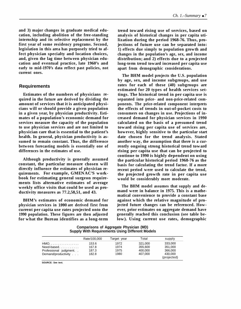
The BHM model assumes that supply and de-mand were in balance in 1975. This is a mathe-matical convenience to provide a constant baseagainst which the relative magnitude of pro-jected future changes can be referenced. How-ever, prior estimates on aggregate demand havegenerally reached this conclusion (see table be-low). Using current use rates, demographic
Comparisons of Aggregate Physician (MD)Supply With Requirements Using Different Models
Rate/100,000 Target year Total supply
HMO. . . . . . . . . . . . . . . . . 153.6 1972 321,000 333,000Need-based. . . . . . . . . . . 167.8 1974 355,600 351,000Professional judgment. . 187.3 1975 400,000 366,000Demand/productivity . . . 182.8 1980 407,000 430,000
(projected)
SOURCE: See text.
.., — —.—. .—. ..—.—
8 ● Forecasts of Physician Supply and Requirements
changes (population increases plus changes inage, sex, and income distribution) are projectedto lead to a lo-percent increase by 1990 over1975 demand, or 415,000 physicians in 1990versus 378,000 in 1975.
Using a trend factor of increasing use basedon 1968-76 data, an additional increase of185,000 in physician demand is projected.
Thus, the total projected demand for physi-cians in 1990 is 600,000 (415,000 PIUS 185,000).a
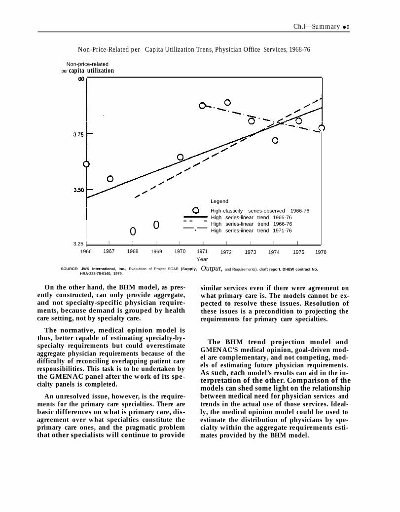
Increases in demand attributable to a histor-ical trend toward increased per capita use areoverestimated, particularly for office services.The period 1968-76 is used to establish thetrend, but whereas a start date of 1968 yields adistinctly upward trend for physician officeservices, a start date of 1971 yields a downwardtrend (see figure on p. 9).
Based on the BHM model, an alternative approximation of the demand for physician serv-ices in 1990, adjusting only for demographicchanges, and assuming no long-term trendtoward increases in per capita use, would be415,00 physicians, an increase of 37,000 from378,000 in 1975. But use could change, as couldproductivity. To some extent, these are policychoices to be made. If it is considered desirablefor use to rise, for physicians to spend a few ex-tra minutes with each patient, or for physiciansto have shorter workweeks, much of the pro-jected supply of 600,000 physicians in 1990could be appropriate.
As supply is estimated to be 600,000 in 1990,there is a difference of 185,000 physicians be-tween predicted supply and estimated demandin a static situation.
Some flexibility in the model is necessary, forseveral reasons. The enactment of nationalhealth insurance should lead to some increase inthe demand for physician services. Second, phy-sicians currently average longer workweeksthan most of the rest of the labor force. Currentprojections are based on the assumption thatphysician productivity will remain constant to1990, which, in specific terms, means that it isassumed that general surgeons will continue to
average 52-hour patient care workweeks, pedia-tricians so hours, etc. If physicians continued tosee patients at the same rate but shortened theirworkweek, this would have the effect of raisingthe number of physicians required to meet a spe-cific level of demand for physician services.Alternatively, physicians might work the samenumber of hours, but see fewer patients andspend more time with each one. This would alsoraise the number of physicians required to meeta specific level of demand for services. Ac-cording to the National Center for Health Sta-tistics, almost half of all office visits to physi-cians in 1973 and 1977 lasted 10 minutes or less.With smaller patient loads, physicians might beable to use the additional time to provide pa-tients with more information, education, andcounseling and lead to greater patient satisfac-tion with the quality of medical care.
It is therefore necessary to decide how muchof these changes are desirable at the cost thatwill be borne by the society.
The GMENAC normative, medical opinionmodel estimates all diseases and conditions (ondemographic bases such as age and sex) thatshould be treated by physicians and the amountof physician services, on a disease-by-disease orcondition-by-condition basis, that should beprovided.
The theoretical level of use is usually adjusteddownwards to real-world estimates throughconsensus formation techniques. Instead ofquantifying use by health care setting, these esti-mates quantify use on a specialty-by-specialtybasis.
Unlike the BHM model, which can project de-mand year to year (projections now exist up toZOO(I), GMENAC’S current future target is 1990,although its model is capable of providing year-to-year projections. GMENAC’S modeling ef-fort, because its ultimate aim is to providerecommendations on graduate medical educa-tion, professes to be less concerned with ag-gregate requirements. When addressed, aggre-gate requirements will be more of a byproductof the parent GMENAC panel’s consolidatingthe work of the individual specialty panels.
Ch.l—Summary ● 9
Non-Price-Related per Capita Utilization Trens, Physician Office Services, 1968-76
Non-price-relatedper capita utilization
0 - - -0 —.—
Legend
High-elasticity series-observed 1966-76High series-linear trend 1966-76High series-linear trend 1966-76High series-iinear trend 1971-76
3.25 [ I 1 I I i I ! I I
1966 1967 1968 1969 1970 1971 1972 1973 1974 1975 1976Year
SOURCE: JWK International, Inc., Evaluation of Project SOAR (Supply,HRA-232-78-0140, 1979.
On the other hand, the BHM model, as pres-ently constructed, can only provide aggregate,and not specialty-specific physician require-ments, because demand is grouped by healthcare setting, not by specialty care.
The normative, medical opinion model isthus, better capable of estimating specialty-by-specialty requirements but could overestimateaggregate physician requirements because of thedifficulty of reconciling overlapping patient careresponsibilities. This task is to be undertaken bythe GMENAC panel after the work of its spe-cialty panels is completed.
An unresolved issue, however, is the require-ments for the primary care specialties. There arebasic differences on what is primary care, dis-agreement over what specialties constitute theprimary care ones, and the pragmatic problemthat other specialists will continue to provide
Output, and Requirements), draft report, DHEW contract No.
similar services even if there were agreement onwhat primary care is. The models cannot be ex-pected to resolve these issues. Resolution ofthese issues is a precondition to projecting therequirements for primary care specialties.
The BHM trend projection model andGMENAC’S medical opinion, goal-driven mod-el are complementary, and not competing, mod-els of estimating future physician requirements.As such, each model’s results can aid in the in-terpretation of the other. Comparison of themodels can shed some light on the relationshipbetween medical need for physician services andtrends in the actual use of those services. Ideal-ly, the medical opinion model could be used toestimate the distribution of physicians by spe-cialty within the aggregate requirements esti-mates provided by the BHM model.
..— _ . —
10 . Forecasts of Physician Supply and Requirements
The GMENAC model focuses on translating anormative definition of medical need into ap-propriate rates of use of medical services, whilethe BHM model looks on medical care as a “con-sumer good” and treats empirical trends in theuse of medical services as a proxy for economicdemand. If the BHM demand estimates shouldprove significantly greater than the GMENACestimates, this would suggest that there arepowerful factors at work that are pushing theuse of medical services beyond the level med-ically necessary and appropriate for “good”care. This would then raise the policy questionof what percentage of the projected future eco-nomic demand for medical services over andabove the professional judgment-based esti-mates of medical need should be considered le-gitimate. Conversely, if the BHM demand esti-mates should prove significantly less than theGMENAC estimates, this would suggest thatthere remains and will remain in the near futuresignificant barriers to obtaining medically nec-essary care for large segments of the Americanpopulation rather than for a few discrete areasand populations. Presumably, these barrierscould be financial, geographic, cultural, or in-volve ignorance about when to seek care—mostlikely some mixture of these variables thatwould need to be investigated. Finally, if theBHM and GMENAC estimates prove to be inrough parity-what could be viewed as the mostdesirable outcome—this would suggest that theeconomic demand for services is more or less inline with professional estimates of the medicalneed for physician services.
As the GMENAC model has yet to generateany numbers, we cannot say which of thesethree alternatives will prove to be the case. Wecan say, however, that the most likely oc-currence would appear to be rough parity or aBHM demand estimate that is significantlygreater than the GMENAC aggregate estimate.The major reason for anticipating that the BHMestimate will most likely prove greater than orat least equal to the GMENAC estimate is thatone of the major variables in the BHM model isa projected trend toward rising per capita use ofmedical services, independent of demographicchanges and projected changes in price. In con-trast, the GMENAC model assumes no major
changes in medical need apart from changes inmedical need induced by demographic shifts(e.g., an aging population) between now and1990; hence, no medical rationale for large percapita increases in the use of physician services.
Estimates of locational requirements are usedto address different problems than aggregateand specialty estimates. Such estimates are usedin operating programs designed to provide phy-sicians and other medical care resources to tar-geted populations. Thus, locational require-ments are based not only on assumptions aboutwhat are appropriate types and quantities ofmedical services, but also on: 1) how medicalservices should be redistributed, and 2) theamount of care that the Federal Governmentshould provide or finance compared to otherpublic and private sources.
These additional assumptions are clearly re-flected in the designation and staffing ratios thatwere used to estimate the numbers of additionalprimary care physicians “needed” in shortageareas, and which, with additional criteria, pro-vide the basis by which specific areas qualify asHMSAS.
Designation ratio. —The actual minimumratio of active, non-Federal, patient carephysicians engaged in primary care to thecivilian population of an area below whichan area is considered to have a shortage ofhealth manpower sufficient to justify itsbeing counted as a shortage area.Staffing ratio. —The theoretical maximumratio if active non-Federal, patient carephysicians engaged in primary care to thecivilian population of an area used as astandard above which an area is consideredto have adequate health manpower so thatadditional Federal intervention with NHSCstaffing is no longer necessary.
The designation ratio reflects that quarter ofthe United States having the least number ofprimary care physicians. It has been set at1:3,500. The staffing ratio establishes a limita-tion on the extent of Federal involvement byspecifying an “appropriate” relationship be-tween the service demands of the populationand the primary care physicians available toprovide these services. It has been set at 1:2,000.
Ch. 1–Summary ● 1 1
Estimates of shortage areas in 1990 must beconsidered weak for a number of reasons. First,data on patterns of distribution of physiciansaged 32 to 40 in 1974 are used as the base fromwhich projections are made. These data are cur-rently the most recent available. They reflect,however, the conditions and policies of the1960’s. To assume that physicians will continueto follow the same distributional patterns in1990 is to discount the large increases in ag-gregate physician supply and deliberate policyefforts to increase the physician supply in short-age areas that have occurred since the 1960’s.Second, future estimates are based almost en-tirely on county physician-to-population ratios,again due to limitations in available nationaldata. Actual HMSA designation, however,often involves smaller areas that have lowerphysician-to-population ratios than the countyas a whole. Thus, methods for estimating futureurban shortages are especially weak.
In such estimates, potential use divided by ex-pected productivity (ultimately expressed inphysician-to-population ratios) is an inadequateindicator of the targeted population’s use ofphysician services, because average use and pro-ductivity calculated on a national basis can beexpected to deviate from a specific population’suse of specific physician services, and accessproblems (physical, financial, social) aIso deter-mine whether use and productivity estimates arerealized.
Thus, physician-to-population ratios com-prise only part of the eligibility criteria thatmust be met to be designated an HMSA. Addi-tional criteria include meeting specific defini-tions of “a rational area for the delivery of pri-mary care services, ” and when “primary medi-cal care manpower in contiguous areas are over-utilized, excessively distant, or inaccessible tothe population of the area under consideration.”
Consequently, even if national aggregate andspecialty requirements were satisfied, it wouldbe unlikely that physicians would be evenly dis-tributed in all geographic areas or equally acces-sible to all population groups. Thus, some areaswould always be underserved as measured
against the average national physician-to-popu-lation ratio.
Projections of supply and requirements de-pend on historical data to predict future events,but legislation in this area has purposely tried toaffect physician specialty and location choices.Given the lag time between medical educationand eventual practice, even recent historicaldata reflect past policies, not current ones.
As currently published, the projections of ag-gregate requirements from BHM give no indica-tion of the very different results that could beobtained by simply shifting the first years of thehistorical period used to establish the trend inper capita use from 1968 to 1971. Assumptionssuch as these are now hidden in the methodol-ogy, yet it is clear that they are crucial to theresults.
Second, these estimates may be given inbasic, high, and low projections or encompass arange of numbers, but they all revolve aroundthe same set of assumptions. They are tech-niques that represent the degree of statisticalconfidence the methodologists have in theircalculations, which is an entirely different ques-tion from projecting alternate estimates basedon fundamentally different sets of assumptionsabout the factors that influence future supplyand requirements.
The final and most important observation isthat the forecasting process has remained tootechnical a process, where statistical techniques,economic knowledge, and medical expertisegreatly influence the process. Yet, more oftenthan not, the basic assumptions adopted in themethodologies are policy ones. This is particu-larly true for projections of the future supply ofphysicians and decisions on specialty distribu-tion requirements. Further, policies that havebeen made and are under consideration directlyimpact on the projections, yet the reliance onhistorical data can systematically underestimatethe effects of such policies. Methodologiststhemselves, in the absence of specific policydirection, are having to make decisions onwhich policies will most directly influence their

. . — . .— -.. ..— —-. —. -— ..-. — ———. .— . . —
— .
12Ž Forecasts of Physician Supply and Requirements
projections. The result is that current forecast-ing techniques may influence policy decisions toa greater extent than called for.
Greater awareness of the limits of forecastingand less preoccupation with a particular set of
numbers would be possible if the assumptionsunderlying the projections are made more ex-plicit; alternative forecasts are projected, basedon different sets of assumptions; and participa-tion in the forecasting process is expanded to in-clude policymakers as well as technicians.

2 m
supply
.
2Supply
This chapter summarizes supply projections for physicians—doctors of medicine(MD) and doctors of osteopathy (DO)-in the aggregate, by specialty, and by loca-tion. The elements to be covered are: 1) assumptions, 2) data sources, and 3) projec-tions.
AGGREGATE SUPPLY
The future aggregate supply of physicians isbased on assumptions of the following factors(USDHEW, 1979a):
● physicians currently active in practice,. new graduates of U.S. medical and osteo-
pathic schools, and. immigration of physicians (including U.S.
citizens studying abroad) educated in othercountries.
The estimates based on these production fac-tors assume that supply will not be affected bythe demand for physicians; i.e., there is an in-elastic relationship between physician produc-tion and demand.
Data on currently active physicians are ob-tained from the American Medical Association(AMA) and the American Osteopathic Associa-tion (AOA). Both AMA and AOA data rely onthe physician’s self-designation of specialty, sothe published data are based on this self-iden-tification of primary specialty and activity andprovide no information on activities in otherspecialty areas nor on the proportion of timespent in actual patient care.
An additional factor is that the “not clas-sified” category in the AMA data, introduced in1971, has grown from 300 in 1971 to over30,000 in 1976, plus approximately 8,800 physi-cians whose addresses were unknown. Seventypercent of this “not classified” category is belowage 35 and most likely in active practice. In thetrend analysis for estimating specialty distribu-tion, this “not classified” category is not in-
cluded. However, “not classified” is included inthe aggregate projections, with the assumptionthat its specialty distribution is identical tophysicians in residency programs.
For physicians currently active in practice,the starting point (base year) is 1974. Data forMDs include age, specialty, and country ofmedical education. DO data for 1974 start with1971 AOA data and add new DOS and subtractretirements and deaths between 1971 and 1974.
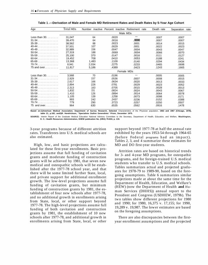
Mortality and retirement rates for MDs arecomputed by age and sex as derived fromstudies on the physician population, not thegeneral population. 1967 data on retirementrates are used, and mortality rates use an articlepublished in 1975. These rates are also appliedto osteopathic physicians. Both retirement andmortality data, therefore, do not reflect trendsthat might be occurring. Table 1 summarizesthese estimates.
Trends in new graduates of U.S. medical andosteopathic schools start with estimates of first-year enrollments to arrive at the number ofgraduates per year after adjustments for attri-tion. 1974 data were the original starting point,but data from the latest academic year, 1977-78,are now used.
Estimates of first-year enrollments are basedon trends in: 1) Federal cavitation support, 2)Federal construction grants activity, 3) newschools already planned, and 4) potential Stateand local support of new schools. Separate com-putations are made for first-year enrollments in
15
16 ● Forecasts of Physician Supply and Requirements
Table 1 .—Derivation of Male and Female MD Retirement Rates and Death Rates by 5-Year Age Cohort
Age Total MDs Number inactive Percent inactive Retirement rate Death rate Separation rate
Male MDs
Less than 30. . . . . . . .31-34 . . . . . . . . . . . . . .35-39 . . . . . . . . . . . . . .40-44 . . . . . . . . . . . . . .45-49 . . . . . . . . . . . . . .50-54 . . . . . . . . . . . . . .55-59 . . . . . . . . . . . . . .60-64 . . . . . . . . . . . . . .65-69 . . . . . . . . . . . . . .70-74 . . . . . . . . . . . . . .75 and over. . . . . . . . .
31,04739,47038,56237,50132,98927,31925,10019,45213,3688,941
11,817
646488
107156188370708
1,4832,0345,186
.0020
.0016
.0023
.0029
.0047
.0069
.0147
.0410
.1109
.2275
.4389
—.0000.0001.0001.0004.0004.0016.0053.0140.0233.0423
.0007
.0007
.0014
.0022
.0043
.0066
.0111
.0188
.0294
.0465
.1243
.0007
.0007
.0015
.0023
.0047
.0070
.0127
.0241
.0434
.0698
.1665
Female MDs
Less than 30. . . . . . . . 3,568 70 .0196 — .0005 .000531-34 . . . . . . . . . . . . . . 2,929 157 .0536 .0007 .0008 .001535-39 . . . . . . . . . . . . . . 2,617 166 .0634 .0020 .0013 .003340-44 . . . . . . . . . . . . . . 2,894 226 .0781 .0029 .0023 .005245-49 . . . . . . . . . . . . . . 2,313 163 .0705 .0015 .0028 .001350-54 . . . . . . . . . . . . . . 1,832 151 .0824 .0024 .0043 .006755-59 . . . . . . . . . . . . . . 1,410 126 .0894 .0014 .0064 .007860-64 . . . . . . . . . . . . . . 1,105 139 .1258 .0073 .0098 .017165-69 . . . . . . . . . . . . . . 993 242 .2437 .0236 .0152 .038870-74 . . . . . . . . . . . . . . 779 290 .3723 .0257 .0250 .050775 and over. . . . . . . . . 964 630 .6535 .0562 .0916 .1478
Based on:1)Amerlcan Medical Association, Department of Survey Research, Selected Characteristics of the Physician population, 1963 and 1967 (Chicago, 1978),table 21, p.182; and2)R. Hendrickson, ’’Specialists Outlive Generalists:’ Prism, December 1975.
SOURCE: Interim Report of the Graduate Medical Education National Advisory Committee to the Secretary, Department of Health, Education, and Welfare, Washington,D. C.: Health Resources Administration, DHEW publication No. (HRA) 79-833, p. 119.
3-year programs because of different attritionrates. Transferees into U.S. medical schools arealso estimated.
High, low, and basic projections are calcu-lated for these first-year enrollments. Basic pro-jections assume that full funding of cavitationgrants and moderate funding of constructiongrants will be achieved by 1981, that seven newmedical and osteopathic schools will be estab-lished after the 1977-78 school year, and thatthere will be some limited further State, local,and private support for additional enrollmentgrowth. The low-level projections assume fullfunding of cavitation grants, but minimumfunding of construction grants by 1981, the es-tablishment of four new schools after 1977-78,and no additional growth in enrollments arisingfrom State, local, or other support beyond1977-78. The high-level projections assume fullfunding of both cavitation and constructiongrants by 1981, the establishment of 10 newschools after 1977-78, and additional growth inenrollments arising from State, local, or other
support beyond 1977-78 at half the annual rateexhibited by the years 1953-54 through 1964-65(before Federal programs had an impact).Tables 2, 3, and 4 summarize these estimates forMD and DO first-year students.
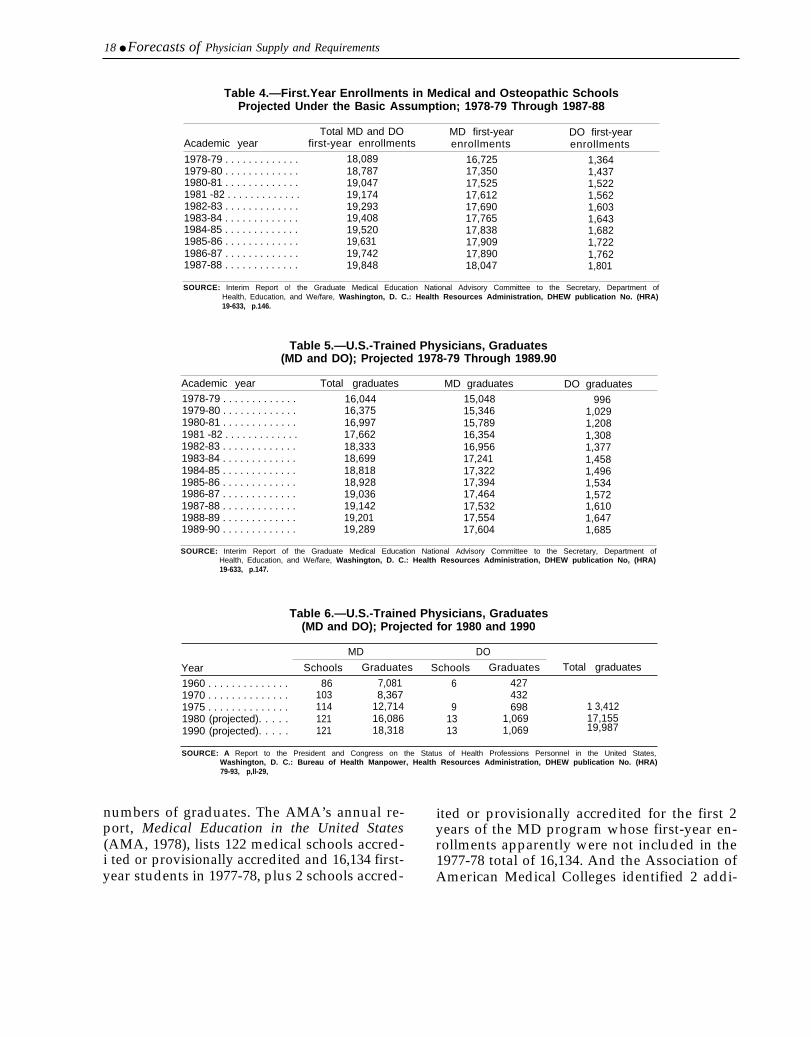
Attrition rates are based on historical trendsfor 3- and 4-year MD programs, for osteopathicprograms, and for foreign-trained U.S. medicalstudents who transfer to U.S. medical schools.Tables summarizes actual and projected gradu-ates for 1978-79 to 1989-90, based on the fore-going assumptions. Table 6 summarizes similarprojections made at about the same time for theDepartment of Health, Education, and Welfare’s(HEW) (now the Department of Health and Hu-man Services (DHHS)) annual report to thePresident and Congress (USDHEW, 1979b). Thetwo tables show different projections for 1980and 1990; for 1980, 16,375 v. 17,155; for 1990,19,289 v. 19,987. The lower estimates are basedon the foregoing assumptions.
There are also discrepancies between the first-year enrollment assumptions and the projected
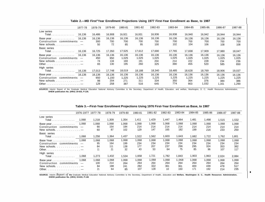
Table 2.—MD First”Year Enrollment Projections Using 1977 First-Year Enrollment as Base, to 1987
1977-78 1978-79 1979-80 1980-81 1981-82 1982-83 1983-84 1984-85 1985-86. 1986-87 1987-88
Low seriesTotal . . . . . . . . . . . . . . . 16,136 16,486 16,908 16,921 16,931 16,936 16,938 16,940 16,942 16,944 16,944
Base year . . . . . . . . . . . . . . . 16,136 16,136 16,136 16,136 16,136 16,136 16,136 16,136 16,136 16,136 16,136Construction commitments — 300 700 700 700 700 700 700 700 700 700New schools. . . . . . . . . . . . . — 50 72 85 95 100 102 104 106 108 108Basic series
Total . . . . . . . . . . . . . . . 16,136 16,725 17,350 17,525 17,612 17,690 17,765 17,838 17,909 17,980 18,047
Base year . . . . . . . . . . . . . . . 16,136 16,136 16,136 16,136 16,136 16,136 16,136 16,136 16,136 16,136 16,136Construction commitments — 450 950 1,025 1,025 1,025 1,025 1,025 1,025 1,025 1,025New schools . . . . . . . . . . . . . — 74 134 169 191 204 214 222 228 234 236Other . . . . . . . . . . . . . . . . . . . — 65 130 195 260 325 390 455 520 585 650High series
Total . . . . . . . . . . . . . . . 16,136 17,013 17,748 18,019 18,188 18,340 18,485 18,628 18,769 18,906 19,037Base year . . . . . . . . . . . . . . . 16,136 16,136 16,136 16,136 16,136 16,136 16,136 16,136 16,136 16.136 16.136Construction commitments — 650 1,150 1,225 1,225 1,225 1,225 1,225 1,225 1,225 1,225New schools . . . . . . . . . . . . . — 98 204 271 311 334 350 364 376 384 386Other . . . . . . . . . . . . . . . . . . . — 129 258 387 516 645 774 903 1,032 1,161 1,290
SOURCE: Interim Report of the Graduate Medical Education National Advisory Committee to the Secretary, Department of Health, Education, and welfare, Washington, D. C.: Health Resources Administration,DHEW publication No. (HRA) 19-633, P.135.
Table 3.—First-Year Enrollment Projections Using 1976 First-Year Enrollment as Base, to 1987
1976-1977 1977-78 1978-79 1979-80 1980-81 1981-82 1982-83 1983-84 1984-85 1985-86 1986-87 1987-88
Low seriesTotal . . . . . . . . . . . . . . . 1,068 1,218 1,309 1,354 1,411 1,429 1,447 1,464 1,481 1,498 1,515 1,532
Base year . . . . . . . . . . . . . . . 1,068 1,068 1,068 1,068 1,068 1,068 1,068 1,068 1,068 1,068 1,068 1,068Construction commitments — 90 154 184 214 214 214 214 214 214 214 214New schools. . . . . . . . . . . . . — 60 87 102 129 147 165 182 199 216 233 250Basic series
Total . . . . . . . . . . . . . . . 1,068 1,258 1,364 1,437 1,522 1,562 1,603 1,643 1,682 1,722 1,762 1,801
Base Year . . . . . . . . . . . . . . . 1,068 1,068 1,068 1,068 1,068 1,068 1,068 1,068 1,068 1,068 1,068 1,068Construction commitments — 95 164 199 234 234 234 234 234 234 234 234New schools. . . . . . . . . . . . . — 84 111 138 177 207 237 266 295 324 353 382Other. . . . . . . . . . . . . . . . . . . — 11 21 32 43 53 64 75 85 96 107 117High series
Total . . . . . . . . . . . . . . . 1,068 1,273 1,432 1,534 1,658 1,721 1,782 1,843 1,903 1,963 2,024 2,084
Base year . . . . . . . . . . . . . . . 1,068 1,068 1,068 1,068 1,068 1,068 1,068 1,068 – 1,068 1,068 1,068 1,068Construction commitments — 100 214 264 264 264 264 264 264 264 264 264New schools. . . . . . . . . . . . . — 84 188 241 282 322 361 361 400 439 478 517Other. . . . . . . . . . . . . . . . . . . — 21 64 85 107 128 10 150 171 192 214 235
SOURCE: Interim Report of the Graduate Medical Education National Advisory Committee to the Secretary, Department of Health, .Education and Welfare, Washington D. C.. Health Resources Administration,●
DHEW publication No. (HRA) 19-633, P.136
—
18 ● Forecasts of Physician Supply and Requirements
Table 4.—First.Year Enrollments in Medical and Osteopathic SchoolsProjected Under the Basic Assumption; 1978-79 Through 1987-88
Total MD and DO MD first-year DO first-yearAcademic year first-year enrollments enrollments enrollments1978-79 . . . . . . . . . . . . . 18,089 16,725 1,3641979-80 . . . . . . . . . . . . . 18,787 17,350 1,4371980-81 . . . . . . . . . . . . . 19,047 17,525 1,5221981 -82 . . . . . . . . . . . . . 19,174 17,612 1,5621982-83 . . . . . . . . . . . . . 19,293 17,690 1,6031983-84 . . . . . . . . . . . . . 19,408 17,765 1,6431984-85 . . . . . . . . . . . . . 19,520 17,838 1,6821985-86 . . . . . . . . . . . . . 19,631 17,909 1,7221986-87 . . . . . . . . . . . . . 19,742 17,890 1,7621987-88 . . . . . . . . . . . . . 19,848 18,047 1,801
SOURCE: Interim Report o! the Graduate Medical Education National Advisory Committee to the Secretary, Department ofHealth, Education, and We/fare, Washington, D. C.: Health Resources Administration, DHEW publication No. (HRA)19-633, p.146.
Table 5.—U.S.-Trained Physicians, Graduates(MD and DO); Projected 1978-79 Through 1989.90
Academic year Total graduates MD graduates DO graduates1978-79 . . . . . . . . . . . . . 16,044 15,048 9961979-80 . . . . . . . . . . . . . 16,375 15,346 1,0291980-81 . . . . . . . . . . . . . 16,997 15,789 1,2081981 -82 . . . . . . . . . . . . . 17,662 16,354 1,3081982-83 . . . . . . . . . . . . . 18,333 16,956 1,3771983-84 . . . . . . . . . . . . . 18,699 17,241 1,4581984-85 . . . . . . . . . . . . . 18,818 17,322 1,4961985-86 . . . . . . . . . . . . . 18,928 17,394 1,5341986-87 . . . . . . . . . . . . . 19,036 17,464 1,5721987-88 . . . . . . . . . . . . . 19,142 17,532 1,6101988-89 . . . . . . . . . . . . . 19,201 17,554 1,6471989-90 . . . . . . . . . . . . . 19,289 17,604 1,685
SOURCE: Interim Report of the Graduate Medical Education National Advisory Committee to the Secretary, Department ofHealth, Education, and We/fare, Washington, D. C.: Health Resources Administration, DHEW publication No, (HRA)19-633, p.147.
Table 6.—U.S.-Trained Physicians, Graduates(MD and DO); Projected for 1980 and 1990
MD DO
Year Schools Graduates Schools Graduates Total graduates
1960 . . . . . . . . . . . . . . 86 7,081 6 4271970 . . . . . . . . . . . . . . 103 8,367 4321975 . . . . . . . . . . . . . . 114 12,714 9 698 1 3,4121980 (projected). . . . . 121 16,086 13 1,069 17,1551990 (projected). . . . . 121 18,318 13 1,069 19,987
SOURCE: A Report to the President and Congress on the Status of Health Professions Personnel in the United States,Washington, D. C.: Bureau of Health Manpower, Health Resources Administration, DHEW publication No. (HRA)79-93, p,ll-29,
numbers of graduates. The AMA’s annual re- ited or provisionally accredited for the first 2port, Medical Education in the United States years of the MD program whose first-year en-(AMA, 1978), lists 122 medical schools accred- rollments apparently were not included in thei ted or provisionally accredited and 16,134 first- 1977-78 total of 16,134. And the Association ofyear students in 1977-78, plus 2 schools accred- American Medical Colleges identified 2 addi-
Ch. 2–Supply ● 1 9
tional medical schools in 1979, for a total of 126(American Medical News, 1979). The projec-tions of first-year enrollments for 1977-78 matchthe AMA’s estimates of the number of first-yearenrollees in medical school (16,136 v. 16,134).But the projections to 1980 and 1990 (table 6)state that there will be 121 medical schools and13 osteopathic schools, compared to 114 medi-cal schools and 9 osteopathic schools in 1975.Thus, it is not clear whether the alternativeestimates of 7, 4, or 10 new medical and osteo-pathic schools include some of the 122 medicalschools already in existence, or whether theyrepresent additional schools, as the explanationof the methodology seems to say.
In addition, the assumption of full cavitationfunding by 1981 also is unrealistic, and the pro-jections also seem to indicate that full cavitationis expected to be maintained after 1981, Cur-rently, the issue with cavitation is whether itwill continue at all, not whether fully author-ized levels will be appropriated.
Immigration of graduates of foreign medicalschools are calculated separately for Canadianmedical graduates (CMGS) and other foreignmedical graduates (FMGs). The Canadian addi-tion is currently estimated to equal losses fromdeath, retirement, and emigration because therecent historical growth has leveled off.
Additions from the rest of FMGs are particu-larly uncertain at this time because of the cur-tailing legislation in the Health Professions Edu-cational Assistance Act of 1976 (Public Law94-484). Since historical trends will not be pre-dictive of future additions to supply by FMGs,the 1974-76 period has been used, with majoradjustments that essentially try to guess at theimpact of the legislative changes. Temporary-visa FMGs are assumed to equal the number ofgraduate medical positions available to themthrough regulations that implement Public Law94-484, which require a stepwise reduction inpositions until available positions to FMGsreach zero by 1990. The addition of permanent-visa FMGs to the supply is based on estimates ofthe number of FMGs passing the National Boardof Medical Examiners’ Visa Qualifying Exam-ination. This exam was begun in September1977, so only 1 or 2 years of data are available.
Permanent-visa FMGs and the proportion oftemporary-visa FMGs estimated to establishpermanent status through marriage (based onactual trends) are assumed to have the samedeath and retirement rates as U.S.-educatedphysicians.
Of crucial importance is the apparent lack ofanalysis of the contribution from U.S. citizensstudying medicine abroad, a situation currentlyunder study by the General Accounting Office.The projections do account for students return-ing to the United States to complete theirmedical education in the United States, but theycomprise only a small part of the pool of U.S.citizens studying medicine abroad.
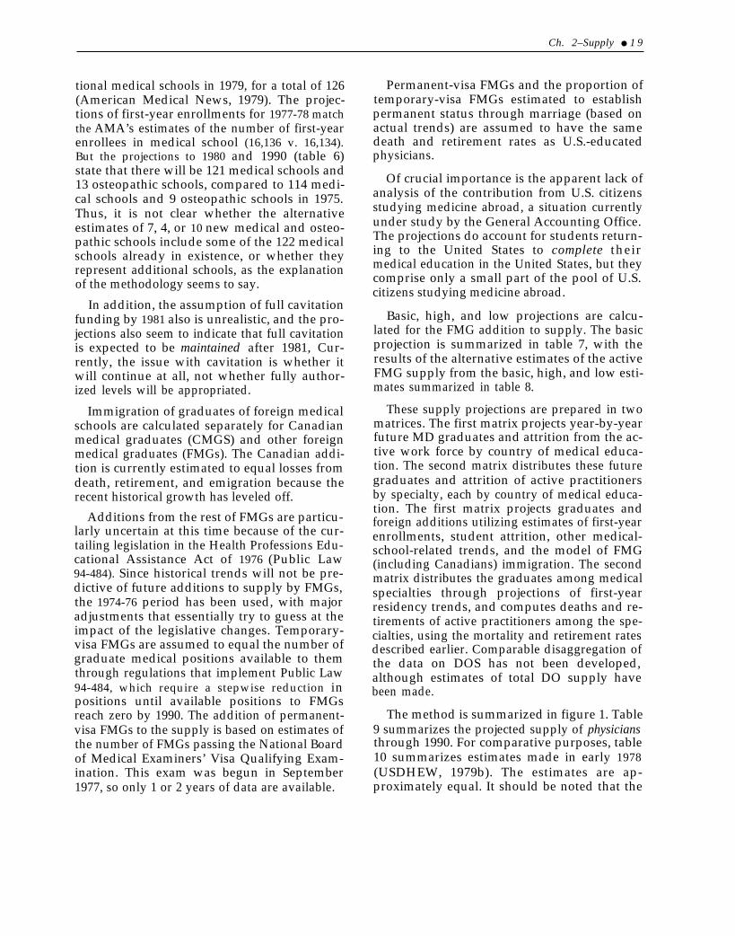
Basic, high, and low projections are calcu-lated for the FMG addition to supply. The basicprojection is summarized in table 7, with theresults of the alternative estimates of the activeFMG supply from the basic, high, and low esti-mates summarized in table 8.
These supply projections are prepared in twomatrices. The first matrix projects year-by-yearfuture MD graduates and attrition from the ac-tive work force by country of medical educa-tion. The second matrix distributes these futuregraduates and attrition of active practitionersby specialty, each by country of medical educa-tion. The first matrix projects graduates andforeign additions utilizing estimates of first-yearenrollments, student attrition, other medical-school-related trends, and the model of FMG(including Canadians) immigration. The secondmatrix distributes the graduates among medicalspecialties through projections of first-yearresidency trends, and computes deaths and re-tirements of active practitioners among the spe-cialties, using the mortality and retirement ratesdescribed earlier. Comparable disaggregation ofthe data on DOS has not been developed,although estimates of total DO supply havebeen made.
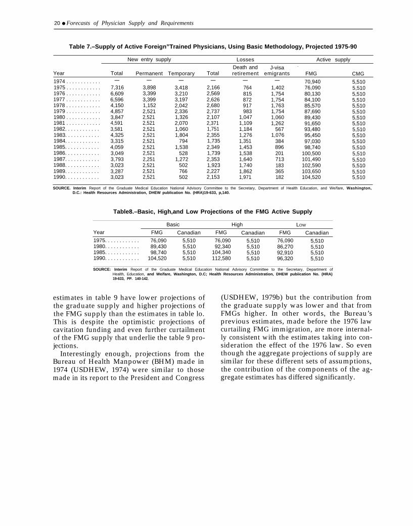
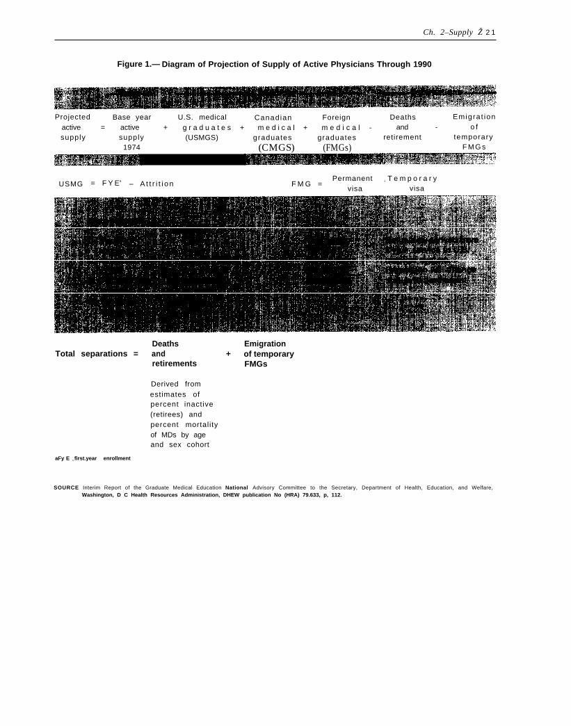
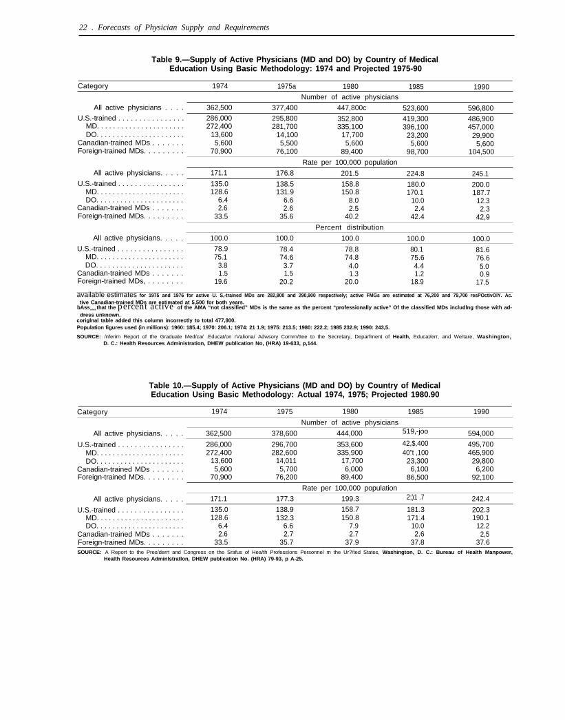
The method is summarized in figure 1. Table9 summarizes the projected supply of physiciansthrough 1990. For comparative purposes, table10 summarizes estimates made in early 1978(USDHEW, 1979b). The estimates are ap-proximately equal. It should be noted that the
20 ● Forecasts of Physician Supply and Requirements
Table 7.–Supply of Active Foreign”Trained Physicians, Using Basic Methodology, Projected 1975-90
New entry supply Losses Active supply
Death and J-visa –
Year Total Permanent Temporary Total retirement emigrants FMG CMG1974 . . . . . . . . . . . .1975 . . . . . . . . . . . .1976 . . . . . . . . . . . .1977 . . . . . . . . . . . .1978 . . . . . . . . . . . .1979 . . . . . . . . . . . .1980 . . . . . . . . . . . .1981 . . . . . . . . . . . .1982. . . . . . . . . . . .1983. . . . . . . . . . . .1984. . . . . . . . . . . .1985. . . . . . . . . . . .1986. . . . . . . . . . . .1987. . . . . . . . . . . .1988. . . . . . . . . . . .1989. . . . . . . . . . . .1990. . . . . . . . . . . .
—7,3166,6096,5964,1504,8573,8474,5913,5814,3253,3154,0593,0493,7933,0233,2873,023
—3,8983,3993,3991,1522,5212,5212,5212,5212,5212,5212,5212,5212,2512,5212,5212,521
—3,4183,2103,1972,0422,3361,3262,0701,0601,804
7941,538
5281,272
502766502
—2,1662,5692,6262,6802,7372,1072,3711,7512,3551,7352,3491,7392,3531,9232,2272,153
—764815872917983
1,0471,1091,1841,2761,3511,4531,5381,6401,7401,8621,971
—1,4021,7541,7541,7631,7541,0601,262
5671,076
384896201713183365182
70,94076,09080,13084,10085,57087,69089,43091,65093,48095,45097,03098,740
100,500101,490102,590103,650104,520
5,5105,5105,5105,5105,5105,5105,5105,5105,5105,5105,5105,5105,5105,5105,5105,5105,510
SOURCE. Interim Report of the Graduate Medical Education National Advisory Committee to the Secretary, Department of Health Education, and We/fare, Washington,D.C.: Health Resources Administration, DHEW publication No. (HRA)19-633, p,140.
Table8.–Basic, High,and Low Projections of the FMG Active Supply
Basic High LOW
Year FMG Canadian FMG Canadian FMG Canadian1975. . . . . . . . . . . . 76,090 5,510 76,090 5,510 76,090 5,5101980. . . . . . . . . . . . 89,430 5,510 92,340 5,510 86,270 5,5101985. . . . . . . . . . . . 98,740 5,510 104,340 5,510 92,910 5,5101990. . . . . . . . . . . . 104,520 5,510 112,580 5,510 96,320 5,510
SOURCE: Interim Report of the Graduate Medical Education National Advisory Committee to the Secretary, Department ofHealth, Education, and We/fare, Washington, D.C; Health Resources Administration, DHEW pubiication No. (HRA)19-633, PP. 140-142.
estimates in table 9 have lower projections ofthe graduate supply and higher projections ofthe FMG supply than the estimates in table lo.This is despite the optimistic projections ofcavitation funding and even further curtailmentof the FMG supply that underlie the table 9 pro-jections.
Interestingly enough, projections from theBureau of Health Manpower (BHM) made in1974 (USDHEW, 1974) were similar to thosemade in its report to the President and Congress
(USDHEW, 1979b) but the contribution fromthe graduate supply was lower and that fromFMGs higher. In other words, the Bureau’sprevious estimates, made before the 1976 lawcurtailing FMG immigration, are more internal-ly consistent with the estimates taking into con-sideration the effect of the 1976 law. So eventhough the aggregate projections of supply aresimilar for these different sets of assumptions,the contribution of the components of the ag-gregate estimates has differed significantly.
Ch. 2–Supply Ž 2 1
Figure 1.— Diagram of Projection of Supply of Active Physicians Through 1990
Projected Base year U.S. medical Canadian Foreign Deaths Emigrat ion
active = active + g r a d u a t e s + m e d i c a l + m e d i c a l - and -supply
o fsupply (USMGS) graduates graduates retirement temporary
1974 (CMGS) (FMGs) F M G s
USMG = F Y Ea – A t t r i t i o n F M G =Permanent + T e m p o r a r y
visa visa
Deaths EmigrationTotal separations = and + of temporary
retirements FMGs
Derived fromestimates ofpercent inactive(retirees) andpercent mortalityof MDs by ageand sex cohort
aFy E = first.year enrollment
SOURCE Interim Report of the Graduate Medical Education National Advisory Committee to the Secretary, Department of Health, Education, and Welfare,Washington, D C Health Resources Administration, DHEW publication No (HRA) 79.633, p, 112.
22 . Forecasts of Physician Supply and Requirements
Table 9.—Supply of Active Physicians (MD and DO) by Country of MedicalEducation Using Basic Methodology: 1974 and Projected 1975-90
Category 1974 1975a 1980 1985 1990Number of active physicians
All active physicians . . . . 362,500 377,400 447,800c 523,600 596,800U.S.-trained . . . . . . . . . . . . . . . . 286,000 295,800 352,800 419,300 486,900
MD. . . . . . . . . . . . . . . . . . . . . . 272,400 281,700 335,100 396,100 457,000DO. . . . . . . . . . . . . . . . . . . . . . 13,600 14,100 17,700 23,200 29,900
Canadian-trained MDs . . . . . . . 5,600 5,500 5,600 5,600 5,600Foreign-trained MDs. . . . . . . . . 70,900 76,100 89,400 98,700 104,500
Rate per 100,000 population
All active physicians. . . . . 171.1 176.8 201.5 224.8 245.1U.S.-trained . . . . . . . . . . . . . . . . 135.0 138.5 158.8 180.0 200.0
MD. . . . . . . . . . . . . . . . . . . . . . 128.6 131.9 150.8 170.1 187.7DO. . . . . . . . . . . . . . . . . . . . . . 6.4 6.6 8.0 10.0 12.3
Canadian-trained MDs . . . . . . . 2.6 2.6 2.5 2.4 2.3Foreign-trained MDs. . . . . . . . . 33.5 35.6 40.2 42.4 42,9
Percent distribution
All active physicians. . . . . 100.0 100.0 100.0 100.0 100.0U.S.-trained . . . . . . . . . . . . . . . . 78.9 78.4 78.8 80.1 81.6
MD. . . . . . . . . . . . . . . . . . . . . . 75.1 74.6 74.8 75.6 76.6DO. . . . . . . . . . . . . . . . . . . . . . 3.8 3.7 4.0 4.4 5.0
Canadian-trained MDs . . . . . . . 1.5 1.5 1.3 1.2 0.9Foreign-trained MDs, . . . . . . . . 19.6 20.2 20.0 18.9 17.5
available estimates for 1975 and 1976 for active U. S,-trained MDs are 282,800 and 290,900 respectively; active FMGs are estimated at 76,200 and 79,700 resPOctivOIY. Ac.tive Canadian-trained MDs are estimated at 5,500 for both years.
bAssume5 that the percent active of the AMA “not classified” MDs is the same as the percent “professionally active” Of the classified MDs includlng those with ad-dress unknown.
coriglnal table added this column incorrectly to total 477,800.Population figures used (in millions): 1960: 185.4; 1970: 206.1; 1974: 21 1.9; 1975: 213.5; 1980: 222.2; 1985 232.9; 1990: 243,5.
SOURCE: /nferirn Report of tfre Graduate Med/ca/ .Educat/on rValiona/ Adwsory Cornrn/ttee to the Secretary, Deparfrnent of Health, Educat/err, and We/tare, Washington,D. C.: Health Resources Administration, DHEW publication No, (HRA) 19-633, p,144.
Table 10.—Supply of Active Physicians (MD and DO) by Country of MedicalEducation Using Basic Methodology: Actual 1974, 1975; Projected 1980.90
Category 1974 1975 1980 1985 1990
Number of active physicians
All active physicians. . . . . 362,500 378,600 444,000 519,-joo 594,000
U.S.-trained . . . . . . . . . . . . . . . . 286,000 296,700 353,600 42,$,400 495,700MD. . . . . . . . . . . . . . . . . . . . . . 272,400 282,600 335,900 40”t ,100 465,900DO. . . . . . . . . . . . . . . . . . . . . . 13,600 14,011 17,700 23,300 29,800
Canadian-trained MDs . . . . . . . 5,600 5,700 6,000 6,100 6,200Foreign-trained MDs. . . . . . . . . 70,900 76,200 89,400 86,500 92,100
Rate per 100,000 population
All active physicians. . . . . 171.1 177.3 199.3 2;)1 .7 242.4
U.S.-trained . . . . . . . . . . . . . . . . 135.0 138.9 158.7 181.3 202.3MD. . . . . . . . . . . . . . . . . . . . . . 128.6 132.3 150.8 171.4 190.1DO. . . . . . . . . . . . . . . . . . . . . . 6.4 6.6 7.9 10.0 12.2
Canadian-trained MDs . . . . . . . 2.6 2.7 2.7 2.6 2,5Foreign-trained MDs. . . . . . . . . 33.5 35.7 37.9 37.8 37.6SOURCE: A Report to the Pres/derrt and Congress on the Srafus of Hea/th ProfessIons Personnel m the Ur?/ted States, Washington, D. C.: Bureau of Health Manpower,
Health Resources Adminlstratlon, DHEW publication No. (HRA) 79-93, p A-25.
Ch. 2–Supply “ 23
SPECIALTY SUPPLY
Recall that aggregate supply was prepared intwo matrices. The first matrix projects grad-uates and foreign additions utilizing estimates offirst-year enrollments, student attrition, othermedical-school-related trends, and the model ofFMG immigration. The second matrix distrib-utes the graduates among medical specialtiesthrough projections of first-year residencytrends, and computes deaths and retirements ofactive practitioners among the specialties.
Comparable disaggregation of the data onDOS has not been developed, although esti-mates of total DO supply have been made. TheDO distribution between primary care special-ties is difficult to predict because of the lack ofbasic data on graduate training positions andbecause the graduate osteopathic training sys-tem is changing. In addition, MD residency pro-grams accept DOS, which could lead to increas-ing specialization by younger DOS.
Presently, about 58 percent of DOS are inprimary care. If DO graduates enter first-yearresidency programs in the same proportion asprojected for MDs, by 1990 only 52 percentwould be in primary care. If DOS continue cur-rent trends in graduate osteopathic training, 64percent would be in primary care in 1990(USDHEW, 1979b). Although these are signifi-cant percentage differences, the absolute dif-ferences are not large. Out of a total DO supplyof 30,000 in 1990, the 52-percent figure cor-responds to about IS, SOO primary care DOS,and the 64-percent figure corresponds to 19,000.This is in contrast to 1990 estimates of total MDand DO supply of 600,000 and a primary careMD supply of 240,000.
The projections for MD speciaIty distributionof the aggregate supply depend principally onfirst-year residency trends and on the attritionrates of the various specialties and subspe-cialties.
The data sources for current specialty supplyare summarized intions are obtainedBoard certificationmemberships. The
table 11. Specialty designa-from the AMA master file,data, and specialty societyAMA file contains self-des-
ignation of specialty, tending to overestimatespecialty supply and underestimate generalpractice supply. And, as only the primary activ-ity/specialty is identified, nothing is knownabout patient care time spent in the identifiedspecialty or in activities usually associated withother specialties. About half of the physiciansidentified in the AMA files are not identified inthe Board certification data. Also, Board certifi-cation data and especially society membershipdata result in duplicate counting, as physicianscan belong to more than one specialty board orsociety. There are 22 medical and surgicalboards and over 130 specialty societies.
BHM uses the AMA master file as its basicsource, with the 1974 active supply as the start-ing point.
First-year residency trends, which are used toproject additions of MD graduates (foreign anddomestic) to the specialties, contain threeassumptions: 1) that the first-year residencydistributions for 1968, 1970-74, and 1976, canbe used to predict future first-year residencytrends; 2) that first-year residency counts forparticular specialties are duplicative in the sensethat a proportion of these residents do not go onto complete that specialty training, but move onto subspecialization or to another specialtyaltogether; and 3) that some residency positionsare shared by different institutions, which alsoleads to duplicative counting. Considering thekinds of interpretation problems that accom-pany trying to project specialty distributionamong active practitioners from first-year resi-dency positions, the better method would be toanalyze final-year residency counts, but theAMA does not keep year-by-year accounts ofmedical graduates, and first-year residency datarepresent the best available data.
Residency data sources and comments ontheir strengths and limitations are summarizedin table 12. The principal data source is theDirectory of Accredited Residencies.
The particular years chosen to establishtrends, 1968, 1970-74, and 1976, are the mostrecent years on which to base such calculations,
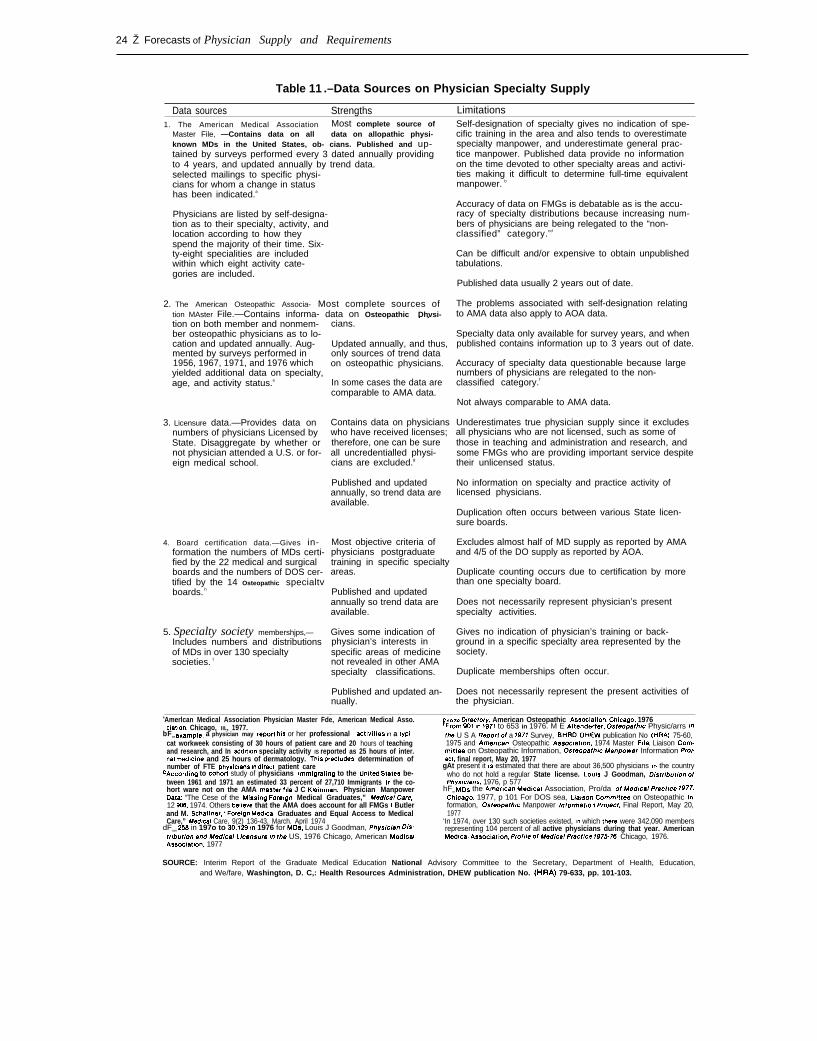
24 Ž Forecasts of Physician Supply and Requirements
Table 11 .–Data Sources on Physician Specialty Supply
Data sources Strengths Limitations1. The American Medical Association Most complete source of
Master File, —Contains data on all data on allopathic physi-known MDs in the United States, ob- cians. Published and up-tained by surveys performed every 3 dated annually providingto 4 years, and updated annually by trend data.selected mailings to specific physi-cians for whom a change in statushas been indicated.a
Physicians are listed by self-designa-tion as to their specialty, activity, andlocation according to how theyspend the majority of their time. Six-ty-eight specialities are includedwithin which eight activity cate-gories are included.
2. The American Osteopathic Associa- Most complete sources oftion MAster File.—Contains informa- data on Osteopathic Dhvsi-tion on both member and nonmem-ber osteopathic physicians as to lo-cation and updated annually. Aug-mented by surveys performed in1956, 1967, 1971, and 1976 whichyielded additional data on specialty,age, and activity status.e
3. Licensure data.—Provides data onnumbers of physicians Licensed byState. Disaggregate by whether ornot physician attended a U.S. or for-eign medical school.
4. Board certification data.—Gives in-formation the numbers of MDs certi-fied by the 22 medical and surgicalboards and the numbers of DOS cer-
. .cians.
Updated annually, and thus,only sources of trend dataon osteopathic physicians.
In some cases the data arecomparable to AMA data.
Contains data on physicianswho have received licenses;therefore, one can be sureall uncredentialled physi-cians are excluded.g
Published and updatedannually, so trend data areavailable.
Most objective criteria ofphysicians postgraduatetraining in specific specialtyareas.
tified by the 14 Osteopathic specialtvboards. h Published and updated
5. Specialty society membershjps,—Includes numbers and distributionsof MDs in over 130 specialtysocieties. t
annually so trend data areavailable.
Gives some indication ofphysician’s interests inspecific areas of medicinenot revealed in other AMAspecialty classifications.
Published and updated an-nually.
Self-designation of specialty gives no indication of spe-cific training in the area and also tends to overestimatespecialty manpower, and underestimate general prac-tice manpower. Published data provide no informationon the time devoted to other specialty areas and activi-ties making it difficult to determine full-time equivalentmanpower. b
Accuracy of data on FMGs is debatable as is the accu-racy of specialty distributions because increasing num-bers of physicians are being relegated to the “non-classified” category.cd
Can be difficult and/or expensive to obtain unpublishedtabulations.
Published data usually 2 years out of date.
The problems associated with self-designation relatingto AMA data also apply to AOA data.
Specialty data only available for survey years, and whenpublished contains information up to 3 years out of date.
Accuracy of specialty data questionable because largenumbers of physicians are relegated to the non-classified category.f
Not always comparable to AMA data.
Underestimates true physician supply since it excludesall physicians who are not licensed, such as some ofthose in teaching and administration and research, andsome FMGs who are providing important service despitetheir unlicensed status.
No information on specialty and practice activity oflicensed physicians.
Duplication often occurs between various State licen-sure boards.
Excludes almost half of MD supply as reported by AMAand 4/5 of the DO supply as reported by AOA.
Duplicate counting occurs due to certification by morethan one specialty board.
Does not necessarily represent physician’s presentspecialty activities.
Gives no indication of physician’s training or back-ground in a specific specialty area represented by thesociety.
Duplicate memberships often occur.
Does not necessarily represent the present activities ofthe physician.
aAmerlcan Medical Association Physician Master Fde, American Medical Asso. ‘1976 D/rectory, American Osteopathic Assoclatlon, Chicago, 1976clatlon, Chicago, III., 1977.
bFor example, a physician may report hfs or her professional activltleS m a tYP1.cat workweek consisting of 30 hours of patient care and 20 hours of teachingand research, and In addltlon specialty activity IS reported as 25 hours of inter.nal medicine and 25 hours of dermatology. This precludas determination ofnumber of FTE phyaiclans m dwect patient care
cAccordlng to cohoti study of physicians Immlgralmg to the United states be-tween 1961 and 1971 an estimated 33 percent of 27,710 Immigrants In the co-hort ware not on the AMA mastar Me J C Klelnman, Physician ManpowerOata. “The Cese of the Mkssmg Foreign Medical Graduates,” Medtcal Care,12 W& 1974. Others beheve that the AMA does account for all FMGs I Butlerand M. Schaffner, “Foreign Medical Graduates and Equal Access to MedicalCare,” Med/ca/ Care, 9(2) 136-43, March. April 1974
dFrom 25s in 197o to 30,129 (n 1976 for MDs, Louis J Goodman, phYSIClan Lk.fr~buflon and Medlca/ Llcerrsura m the US, 1976 Chicago, American MedicalAssoclatlon, 1977
fFrom s01 In 1971 to 653 in 1976. M E Altenderfar, OstaOpath/C Physic/arrs Inthe U S A Reporf of a 1971 Survey, BHRD, DHEW publication No (HRA) 75-60,1975 and Amertcan Osteopathic As.soaatlon, 1974 Master File, Liaison Corn.mlttee on Osteopathic Information, Osteopatfwc Manpowar Information I@ect, final report, May 20, 1977
gAt present it IS estimated that there are about 36,500 physicians In the countrywho do not hold a regular State license. LouIs J Goodman, Ostrdxmon ofPhys)c!ans, 1976, p 577
hFor MDS the American Medical Association, Pro/da of A4edtcal Pr8Ct/Ce 1977,Chtcago, 1977, p 101 For DOS sea, L/awon Commtttea on Osteopathic fmformation, Osteopathic Manpower /rrformat/o? Pro/ect, Final Report, May 20,1977
‘In 1974, over 130 such societies existed, In which thera were 342,090 membersrepresenting 104 percent of all active physicians during that year. AmericanMedical Assoclatlon, Profde of Med/ca/ Pracf/ce 197>76 Chicago, 1976.
SOURCE: Interim Report of the Graduate Medical Education National Advisory Committee to the Secretary, Department of Health, Education,and We/fare, Washington, D. C,: Health Resources Administration, DHEW publication No. (HRA) 79-633, pp. 101-103.
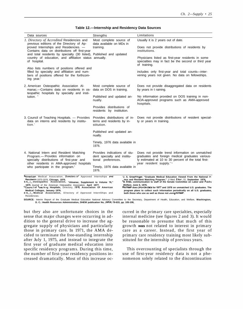
Ch. 2—Supply • 25
Table 12.—lnternship and Residency Data Sources
Data sources Strengths Limitations
1. Directory of Accredited Residencies and Most complete source ofprevious editions of the Directory of Ap- data available on MDs inproved Internships and Residencies. — training.Contains data on distributions off first-yearand total residents by specialty (30 listed), Published and updatedcountry of education, and affiliation status annually.of hospital.
Also lists numbers of positions offered andfilled by specialty and affiliation and num-bers of positions offered for the forthcom-ing year.a
2. American Osteopathic Association Al-manac.—Contains data on residents in os-teopathic hospitals by specialty and insti-tution. b
3. Council of Teaching Hospitals. — Providesdata on interns and residents by institu-tion. c
4. National Intern and Resident MatchingProgram.— Provides information onspecialty distributions of first-year andother residents in AMA-approved hospitalswho participate in the program.d
Most complete source ofdata on DOS in training.
Published and updated an-nually.
Provides distributions ofresidents by institution.
Provides distributions of in-terns and residents by in-stitution.
Published and updated an-nually.
Timely, 1976 data available in1976.
Provides indications of stu-dent specialty and institu-tional preferences.
Timely, 1976 data available in1976.
Usually it is 2 years out of date.
Does not provide distributions of residents byinstitutions.
Physicians listed as first-year residents in somespecialties may in fact be the second or third yearof training.
includes only first-year and total counts—inter-vening years not given. No data on fellowships.
Does not provide disaggregated data on residentsby years in t raining.
No information provided on DOS training in non-AOA-approved programs such as AMA-approvedhospitals.
Does not provide distributions of resident special-ty or years in training.
Does not provide trend information on unmatchedgraduates and foreign medical graduates various-ly estimated at 10 to 30 percent of the total first-year resident supply.e f g
aArnerican Medical Association, L1/recfory of Approved Internships and ‘J. S. Graettinger, “Graduate Medical Education Viewed From the National ln-Resfderrts 1975-1976, Chicago, 1976. tern and Resident Matching Program,” J. Med. Educ,, 51, September 1976,
b Am e rican Osteopathic Association, “Almanac, Supplement to Volume 76,” fB, Biles, communication to staff of the Senate Committee on Labor and Public1975 Journal of the American Osteopathic Association, April 1977. Welfare, June 6, 1976.
ccouncil of Teaching Hospitals, Directory, 1976, Association Of American gNIRMp does provide data for 1977 and 1978 on unmatched U.S. graduates. TheMedical Colleges, January 1976.
d Am e r i can Medical Association, D/rectory of Approved InternShips andprogram plans to collect such information periodically on all U.S. graduates,both those who use as well as those not using NIRMP.
Residencies.
SOURCE: Interim Report of the Graduate Medical Education National Advisory Committee to the Secretary, Department of Health, Education, and Welfare, Washington,D. C.: Health Resources Administration, DHEW publication No, (HRA) 79-633, pp. 105-108,
but they also are unfortunate choices in thesense that major changes were occurring in ad-dition to the general drive to increase the ag-gregate supply of physicians and particularlythose in primary care. In 1971, the AMA de-cided to terminate the free-standing internshipafter July 1, 1975, and instead to integrate thefirst year of graduate medical education intospecific residency programs. During this time,the number of first-year residency positions in-creased dramatically. Most of this increase oc-
curred in the primary care specialties, especiallyinternal medicine (see figures 2 and 3). It wouldbe reasonable to presume that much of thisgrowth was not related to interest in primarycare as a career. Instead, the first year ofprimary care residency training most likely sub-stituted for the internship of previous years.
This overcounting of specialists through theuse of first-year residency data is not a phe-nomenon solely related to the discontinuation
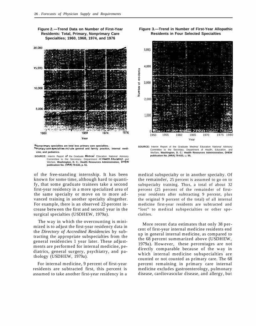
26 . Forecasts of Physician Supply and Requirements
Figure 2. —Trend Data on Number of First-YearResidents: Total, Primary, Nonprimary Care
Specialties; 1960, 1968, 1974, and 1976
Figure 3.—Trend in Number of First-Year AllopathicResidents in Four Selected Specialties
aNOrlprlnlary specialties are total less primary care specialties.bprimav care specialties include general and family practice, internal medi-
cine, and pediatrics.
SOURCE: interim Report of the Graduate Med/cal Education National AdvisoryCommittee to the Secretary, Department of /fea/th, Educat/on, andWe//are, Washington, D. C.: Health Resources Administration, DHEWpublication No. (HRA) 79-633, p. 51.
of the free-standing internship. It has beenknown for some time, although hard to quanti-fy, that some graduate trainees take a secondfirst-year residency in a more specialized area ofthe same specialty or move on to more ad-vanced training in another specialty altogether.For example, there is an observed 22-percent in-crease between the first and second year in thesurgical specialties (USDHEW, 1979a).
The way in which the overcounting is mini-mized is to adjust the first-year residency data inthe Directory of Accredited Residencies by sub-tracting the appropriate subspecialties from thegeneral residencies 1 year later. These adjust-ments are performed for internal medicine, pe-diatrics, general surgery, psychiatry, and pa-thology (USDHEW, 1979a).
For internal medicine, 9 percent of first-yearresidents are subtracted first, this percent isassumed to take another first-year residency in a
5,00(1
4,000
3,000
2,000
1,000
01950 1955 1960 1965 1970 1975 1980
Year
SOURCE: Interim Report of the Graduate Medma/ Education Nat/ona/ AdvisoryCommittee to the Secretary, Department of Hea/th, Educat/on, andWe/fare, Washington, D. C.: Health Resources Administration, DHEWpublication No. (HRA) 79-633, LI. 50,
medical subspecialty or in another specialty. Ofthe remainder, 25 percent is assumed to go on tosubspecialty training. Thus, a total of about 32percent (25 percent of the remainder of first-year residents after subtracting 9 percent, plusthe original 9 percent of the total) of all internalmedicine first-year residents are subtracted and“lost” to medical subspecialties or other spe-cialties.
More recent data estimates that only 38 per-cent of first-year internal medicine residents endup in general internal medicine, as compared tothe 68 percent summarized above (USDHEW,1979a). However, these percentages are notdirectly comparable because of the way inwhich internal medicine subspecialties arecounted or not counted as primary care. The 68percent remaining in primary care internalmedicine excludes gastroenterology, pulmonarydisease, cardiovascular disease, and allergy, but
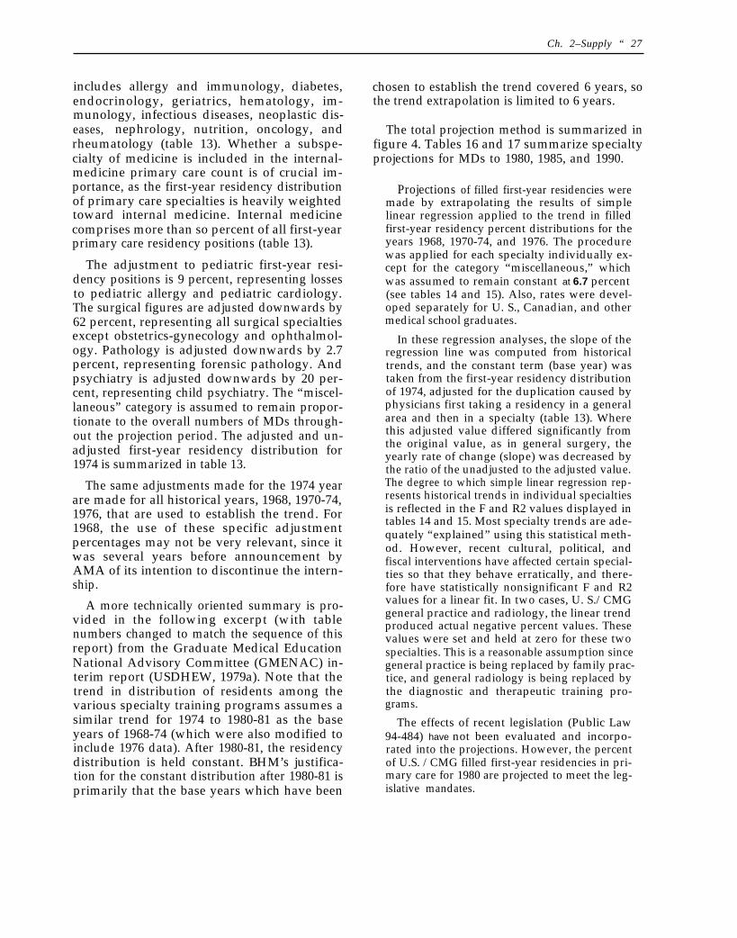
Ch. 2–Supply “ 27
includes allergy and immunology, diabetes,endocrinology, geriatrics, hematology, im-munology, infectious diseases, neoplastic dis-eases, nephrology, nutrition, oncology, andrheumatology (table 13). Whether a subspe-cialty of medicine is included in the internal-medicine primary care count is of crucial im-portance, as the first-year residency distributionof primary care specialties is heavily weightedtoward internal medicine. Internal medicinecomprises more than so percent of all first-yearprimary care residency positions (table 13).
The adjustment to pediatric first-year resi-dency positions is 9 percent, representing lossesto pediatric allergy and pediatric cardiology.The surgical figures are adjusted downwards by62 percent, representing all surgical specialtiesexcept obstetrics-gynecology and ophthalmol-ogy. Pathology is adjusted downwards by 2.7percent, representing forensic pathology. Andpsychiatry is adjusted downwards by 20 per-cent, representing child psychiatry. The “miscel-laneous” category is assumed to remain propor-tionate to the overall numbers of MDs through-out the projection period. The adjusted and un-adjusted first-year residency distribution for1974 is summarized in table 13.
The same adjustments made for the 1974 yearare made for all historical years, 1968, 1970-74,1976, that are used to establish the trend. For1968, the use of these specific adjustmentpercentages may not be very relevant, since itwas several years before announcement byAMA of its intention to discontinue the intern-ship.
A more technically oriented summary is pro-vided in the following excerpt (with tablenumbers changed to match the sequence of thisreport) from the Graduate Medical EducationNational Advisory Committee (GMENAC) in-terim report (USDHEW, 1979a). Note that thetrend in distribution of residents among thevarious specialty training programs assumes asimilar trend for 1974 to 1980-81 as the baseyears of 1968-74 (which were also modified toinclude 1976 data). After 1980-81, the residencydistribution is held constant. BHM’s justifica-tion for the constant distribution after 1980-81 isprimarily that the base years which have been
chosen to establish the trend covered 6 years, sothe trend extrapolation is limited to 6 years.
The total projection method is summarized infigure 4. Tables 16 and 17 summarize specialtyprojections for MDs to 1980, 1985, and 1990.
Projections of filled first-year residencies weremade by extrapolating the results of simplelinear regression applied to the trend in filledfirst-year residency percent distributions for theyears 1968, 1970-74, and 1976. The procedurewas applied for each specialty individually ex-cept for the category “miscellaneous,” whichwas assumed to remain constant at 6.7 percent(see tables 14 and 15). Also, rates were devel-oped separately for U. S., Canadian, and othermedical school graduates.
In these regression analyses, the slope of theregression line was computed from historicaltrends, and the constant term (base year) wastaken from the first-year residency distributionof 1974, adjusted for the duplication caused byphysicians first taking a residency in a generalarea and then in a specialty (table 13). Wherethis adjusted value differed significantly fromthe original vaIue, as in general surgery, theyearly rate of change (slope) was decreased bythe ratio of the unadjusted to the adjusted value.The degree to which simple linear regression rep-resents historical trends in individual specialtiesis reflected in the F and R2 values displayed intables 14 and 15. Most specialty trends are ade-quately “explained” using this statistical meth-od. However, recent cultural, political, andfiscal interventions have affected certain special-ties so that they behave erratically, and there-fore have statistically nonsignificant F and R2values for a linear fit. In two cases, U. S./CMGgeneral practice and radiology, the linear trendproduced actual negative percent values. Thesevalues were set and held at zero for these twospecialties. This is a reasonable assumption sincegeneral practice is being replaced by family prac-tice, and general radiology is being replaced bythe diagnostic and therapeutic training pro-grams.
The effects of recent legislation (Public Law94-484) have not been evaluated and incorpo-rated into the projections. However, the percentof U.S. /CMG filled first-year residencies in pri-mary care for 1980 are projected to meet the leg-islative mandates.
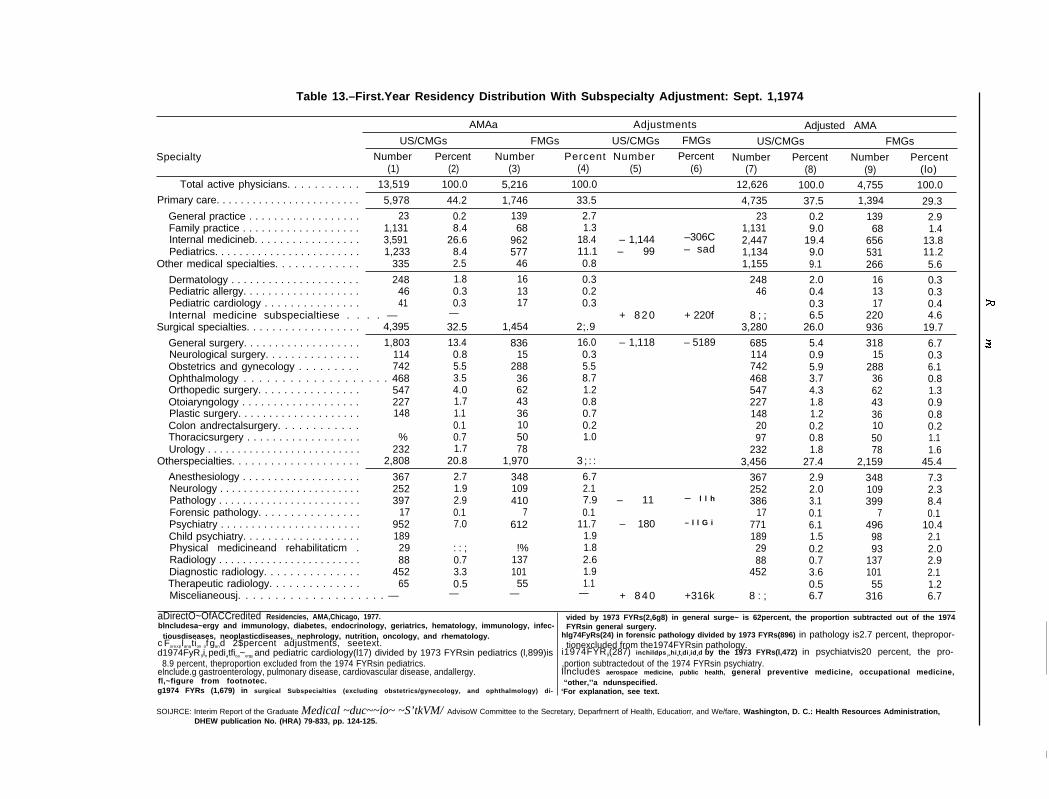
Table 13.–First.Year Residency Distribution With Subspecialty Adjustment: Sept. 1,1974
AMAa Adjustments Adjusted AMA
US/CMGs FMGs US/CMGs FMGs US/CMGs FMGs
Specialty Number Percent Number Percent Number Percent Number Percent Number Percent(1) (2) (3) (4) (5) (6) (7) (8) (9) (lo)
Total active physicians. . . . . . . . . . . 13,519 100.0 5,216 100.0 12,626 100.0 4,755 100.0Primary care. . . . . . . . . . . . . . . . . . . . . . . . 5,978 44.2 1,746 33.5 4,735 37.5 1,394 29.3
General practice . . . . . . . . . . . . . . . . . . 23 0.2 139 2.7 23 0.2 139 2.9Family practice . . . . . . . . . . . . . . . . . . . 1,131 8.4 68 1.3 1,131 9.0 68 1.4Internal medicineb. . . . . . . . . . . . . . . . . 3,591 26.6 962 18.4 – 1,144 –306C 2,447 19.4 656 13.8Pediatrics. . . . . . . . . . . . . . . . . . . . . . . . 1,233 8.4 577 11.1 – 99 – sad 1,134 9.0 531 11.2
Other medical specialties. . . . . . . . . . . . . 335 2.5 46 0.8 1,155 9.1 266 5.6
Dermatology . . . . . . . . . . . . . . . . . . . . . 248 1.8 16 0.3 248 2.0 16 0.3Pediatric allergy. . . . . . . . . . . . . . . . . . . 46 0.3 13 0.2 46 0.4 13 0.3Pediatric cardiology . . . . . . . . . . . . . . . 41 0.3 17 0.3 0.3 17 0.4Internal medicine subspecialtiese . . . . — — + 8 2 0 + 220f 8 ; ; 6.5 220 4.6
Surgical specialties. . . . . . . . . . . . . . . . . . 4,395 32.5 –1,454 2;.9 3,280 26.0 936 19.7
General surgery. . . . . . . . . . . . . . . . . . . 1,803 13.4 836 16.0 – 1,118 – 5189 685 5.4 318 6.7Neurological surgery. . . . . . . . . . . . . . . 114 0.8 15 0.3 114 0.9 15 0.3Obstetrics and gynecology . . . . . . . . . 742 5.5 288 5.5 742 5.9 288 6.1Ophthalmology . . . . . . . . . . . . . . . . . . . 468 3.5 36 8.7 468 3.7 36 0.8Orthopedic surgery. . . . . . . . . . . . . . . . 547 4.0 62 1.2 547 4.3 62 1.3Otoiaryngology . . . . . . . . . . . . . . . . . . . 227 1.7 43 0.8 227 1.8 43 0.9Plastic surgery. . . . . . . . . . . . . . . . . . . . 148 1.1 36 0.7 148 1.2 36 0.8Colon andrectalsurgery. . . . . . . . . . . . 0.1 10 0.2 20 0.2 10 0.2Thoracicsurgery . . . . . . . . . . . . . . . . . . % 0.7 50 1.0 97 0.8 50 1.1Urology . . . . . . . . . . . . . . . . . . . . . . . . . . 232 1.7 78 232 1.8 78 1.6
Otherspecialties. . . . . . . . . . . . . . . . . . . . 2,808 20.8 1,970 3 ; : : 3,456 27.4 2,159 45.4Anesthesiology . . . . . . . . . . . . . . . . . . . 367 2.7 348 6.7 367 2.9 348 7.3Neurology . . . . . . . . . . . . . . . . . . . . . . . . 252 1.9 109 2.1 252 2.0 109 2.3Pathology . . . . . . . . . . . . . . . . . . . . . . . . 397 2.9 410 7.9 – 11 – l l h 386 3.1 399 8.4Forensic pathology. . . . . . . . . . . . . . . . 17 0.1 7 0.1 17 0.1 7 0.1Psychiatry . . . . . . . . . . . . . . . . . . . . . . . 952 7.0 612 11.7 – 180 – l l G i 771 6.1 496 10.4Child psychiatry. . . . . . . . . . . . . . . . . . . 189 1.9 189 1.5 98 2.1Physical medicineand rehabilitaticm . 29 : : ; !% 1.8 29 0.2 93 2.0Radiology . . . . . . . . . . . . . . . . . . . . . . . . 88 0.7 137 2.6 88 0.7 137 2.9Diagnostic radiology. . . . . . . . . . . . . . . 452 3.3 101 1.9 452 3.6 101 2.1Therapeutic radiology. . . . . . . . . . . . . . 65 0.5 55 1.1 0.5 55 1.2Miscelianeousj. . . . . . . . . . . . . . . . . . . . — — — — + 8 4 0 +316k 8 : ; 6.7 316 6.7
aDirectO~OfACCredited Residencies, AMA,Chicago, 1977.blncludesa~ergy and immunology, diabetes, endocrinology, geriatrics, hematology, immunology, infec-
vided by 1973 FYRs(2,6g8) in general surge~ is 62percent, the proportion subtracted out of the 1974FYRsin general surgery.
tiousdiseases, neoplasticdiseases, nephrology, nutrition, oncology, and rhematology. hlg74FyRs(24) in forensic pathology divided by 1973 FYRs(896) in pathology is2.7 percent, thepropor-c Forexplanation of gand 2$percent adjustments, seetext. tionexcluded from the1974FYRsin pathology.d1974FyR9in pediatfica~ergy and pediatric cardiology(l17) divided by 1973 FYRsin pediatrics (l,899)is i1974FYR9(287) inchildps ychiatvdivided by the 1973 FYRs(l,472) in psychiatvis20 percent, the pro-
8.9 percent, theproportion excluded from the 1974 FYRsin pediatrics. ,portion subtractedout of the 1974 FYRsin psychiatry.elnclude.g gastroenterology, pulmonary disease, cardiovascular disease, andallergy. Ilncludes aerospace medicine, public health, general preventive medicine, occupational medicine,fl,~figure from footnotec. “other,’’a ndunspecified.g1974 FYRs (1,679) in surgical Subspecialties (excluding obstetrics/gynecology, and ophthalmology) di- ‘For explanation, see text.
SOIJRCE: Interim Report of the Graduate Medical ~duc~~io~ ~S’tkVM/ AdvisoW Committee to the Secretary, Deparfrnerrt of Health, Educatiorr, and We/fare, Washington, D. C.: Health Resources Administration,DHEW publication No. (HRA) 79-833, pp. 124-125.
I
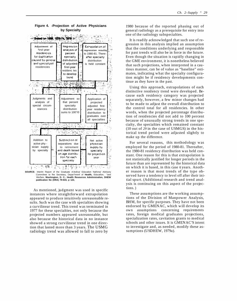
Ch. 2–Supply “ 29
Figure 4. -Projection of Active Physiciansby Specialty
Adjustment of
~G regression results
, :. . to 1980-81. There-
distributionis held constant
residenciesresldenc Ies ~.
, ‘ , . . .
$..;’ $ :, * - , , 1 . ’
Judgments and ““ Adjustment so Application ofanalysis of “ that percent projected
special circum- specialty adjusted first-stances - distribution - year residency
sums to 100°/0 distribution to
.> graduates overall specialties
,
, . .? > . . ‘.,
Addition to Net activeactive phy - separations due
sician supply :. to retirement ,by specialty m
, ,
- . **. q.$j .: ,* -., ,, & ! J ‘: ~. ,. . . 7. . z ‘ , . , . _: . .: .,} . . . +. ! , . . .,; ,i. , ;f ,? ‘‘“SOURCE: Interim Report of the Graduate A.fed/ca/ Education Naf/ona/ Advisory
Cornrn/tree to fhe Secretary, Depar?nrenf of Health, Educaf/on, “andWe/fare, Washington, D. C.. Health Resources Admlnistratlon, DHEWpublication No (HRA) 79-633, p 122,
As mentioned, judgment was used in specificinstances where straightforward extrapolationappeared to produce intuitively unreasonable re-sults. Such was the case with specialties showinga curvilinear trend. This trend was terminated in1977 for these specialties, not only because theprojected numbers appeared unreasonable, butalso because the historical data in no instanceshowed a strong curvilinear trend in one direc-tion that lasted more than 3 years. The USMGradiology trend was allowed to fall to zero by
1980 because of the reported phasing out ofgeneral radiology as a prerequisite for entry intoone of the radiology subspecialties.
It is readily acknowledged that such use of re-gression in this analysis implied an assumptionthat the conditions underlying and responsiblefor past trends will also be in force in the future.Even though the situation is rapidly changing inthe GME environment, it is nonetheless believedthat such projections, when interpreted in a cau-tious manner, can be of value as “baseline” esti-mates, indicating what the specialty configura-tion might be if residency developments con-tinue as they have in the past.
Using this approach, extrapolations of eachdistinctive residency trend were developed. Be-cause each residency category was projectedseparately, however, a few minor changes hadto be made to adjust the overall distribution tothe control total for all residencies. In otherwords, when the projected percentage distribu-tion of residencies did not add to 100 percentbecause of unusually strong trends in one spe-cialty, the specialties which remained constant(10 out of 29 in the case of USMGS) in the his-torical trend period were adjusted slightly tomake up the difference.
For several reasons, this methodology wasemployed for the period of 1980-81. Thereafter,the 1980-81 residency distribution was held con-stant. One reason for this is that extrapolation isnot statistically justified for longer periods in thefuture than are represented by the historical dataon which it is based, in this case 6 years. Anoth-er reason is that most trends of the type ob-served have a tendency to level off after their ini-tial spurt. (Additional research and trend anal-ysis is continuing on this aspect of the projec-tions. )
These assumptions are the working assump-tions of the Division of Manpower Analysis,BHM, for specific purposes. They have not beenendorsed by GMENAC, which will develop itsown assumptions concerning requirementsrates, foreign medical graduates projections,specialization rates, cavitation grants to medicalschools and other issues. It is GMENAC’S intentto investigate and, as needed, modify these as-sumptions (USDHEW, 1979a).
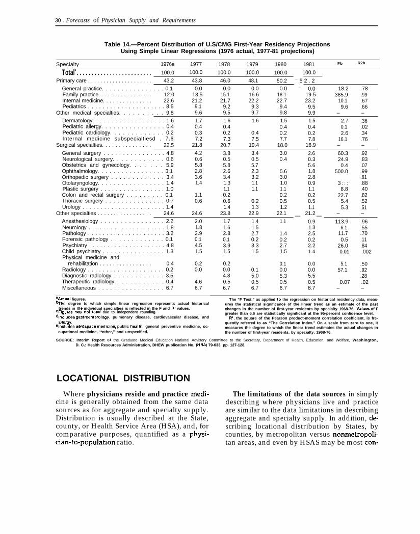
30 . Forecasts of Physician Supply and Requirements
Table 14.—Percent Distribution of U.S/CMG First-Year Residency ProjectionsUsing Simple Linear Regressions (1976 actual, 1977-81 projections)
Specialty 1976a 1977 1978 1979 1980 1981 Fb R2b
Totalc . . . . . . . . . . . . . . . . . . . . . . . . . 100.0 100.0 100.0 100.0 100.0 100.0
Primary care . . . . . . . . . . . . . . . . . . . . . 43.2 43.8 46.0 48.1 50.2 — 5 2 . 2
General practice. . . . . . . . . . . . . . . . 0.1 0.0 0.0 0.0 0.0 — 0.0 18.2 .78Family practice. . . . . . . . . . . . . . . . . 12.0 13.5 15.1 16.6 18.1 19.5 385.9 .99Internal medicine. . . . . . . . . . . . . . . 22.6 21.2 21.7 22.2 22.7 23.2 10.1 .67Pediatrics . . . . . . . . . . . . . . . . . . . . . 8.5 9.1 9.2 9.3 9.4 9.5 9.6 .66
Other medical specialties. . . . . . . . . . 9.8 9.6 9.5 9.7 9.8 9.9 – –
Dermatology. . . . . . . . . . . . . . . . . . . 1.6 1.7 1.6 1.6 1.5 1.5 2.7 .36Pediatric allergy. . . . . . . . . . . . . . . . 0.4 0.4 0.4 0.4 0.4 0.1 .02Pediatric cardiology. . . . . . . . . . . . . 0.2 0.3 0.2 0.4 0.2 0.2 2.6 .34Internal medicine subspecialtiesd . 7.6 7.2 7.3 7.5 7.7 7.8 16.1 .76
Surgical specialties. . . . . . . . . . . . . . . 22.5 21.8 20.7 19.4 18.0 16.9 – –
General surgery . . . . . . . . . . . . . . . . 4.8 4.2 3.8 3.4 3.0 2.6 60.3 .92Neurological surgery. . . . . . . . . . . . 0.6 0.6 0.5 0.5 0.4 0.3 24.9 .83Obstetrics and gynecology. . . . . . . 5.9 5.8 5.8 5.7 5.6 0.4 .07Ophthalmology. . . . . . . . . . . . . . . . . 3.1 2.8 2.6 2.3 5.6 1.8 500.0 .99Orthopedic surgery . . . . . . . . . . . . . 3.4 3.6 3.4 3.2 3.0 2.8 .61Otolaryngology. . . . . . . . . . . . . . . . . 1.4 1.4 1.3 1.1 1.0 0.9 3 : : : .88Plastic surgery . . . . . . . . . . . . . . . . . 1.0 1.1 1.1 1.1 1.1 8.8 .40Colon and rectal surgery . . . . . . . . . 0.1 1.1 0.2 0.2 0.2 22.7 .82Thoracic surgery . . . . . . . . . . . . . . . 0.7 0.6 0.6 0.2 0.5 0.5 5.4 .52Urology . . . . . . . . . . . . . . . . . . . . . . . 1.4 1.4 1.3 1.2 1.1 5.3 .51
Other specialties . . . . . . . . . . . . . . . . . 24.6 24.6 23.8 22.9 22.1 21.2 – –
Anesthesiology . . . . . . . . . . . . . . . . 2.2— —
2.0 1.7 1.4 1.1 0.9 113.9 .96Neurology . . . . . . . . . . . . . . . . . . . . . 1.8 1.8 1.6 1.5 1.3 6.1 .55Pathology . . . . . . . . . . . . . . . . . . . . . 3.2 2.9 2.8 2.7 1.4 2.5 11.7 .70Forensic pathology . . . . . . . . . . . . . 0.1 0.1 0.1 0.2 0.2 0.2 0.5 .11Psychiatry . . . . . . . . . . . . . . . . . . . . . 4.8 4.5 3.9 3.3 2.7 2.2 26.0 .84Child psychiatry . . . . . . . . . . . . . . . . 1.3 1.5 1.5 1.5 1.5 1.4 0.01 .002Physical medicine and
rehabilitation . . . . . . . . . . . . . . . . 0.4 0.2 0.2 0.1 0.0 5.1 .50Radiology . . . . . . . . . . . . . . . . . . . . . 0.2 0.0 0.0 0.1 0.0 0.0 57.1 .92Diagnostic radiology . . . . . . . . . . . . 3.5 4.8 5.0 5.3 5.5 .28Therapeutic radiology . . . . . . . . . . . 0.4 4.6 0.5 0.5 0.5 0.5 0.07 .02Miscellaneous . . . . . . . . . . . . . . . . . 6.7 6.7 6.7 6.7 6.7 6.7 – –
aActual figures.%he degree to which simple linear regression represents actual historical
trends in the individual specialties is reflected in the F and fly values.CFigUreS may not total due to independent rounding.dlncludes gastroenterology, pulmonary disease, cardiovascular disease, and
ailergy.elncludes aerospace n’wdklrre, public heaith, general preventive medicine, oc-
cupational medicine, ‘*other,” and unspecified.
The “F Test,” as applied to the regression on historical residency data, meas-ures the statistical significance of the linear trend as an estimate of the pastchanges in the number of first-year residents by specialty 1968-76. Vaiues of Fgreater than 6.6 are statistically significant at the 95-percent confidence level.
R’, the square of the Pearson product-moment correlation coefficient, is fre-quently referred to as “The Correlation Index.” On a scale from zero to one, itmeasures the degree to which the linear trend estimates the actual changes inthe number of first-year residents, by specialty, 1968-76.
SOURCE: Interim Report of the Graduate Medical Education National Advisory Committee to the Secretary, Department of Health, Education, and Welfare, Washington,D. C.: Health Resources Administration, DHEW publication No. (HRA) 79-633, pp. 127-128.
LOCATIONAL DISTRIBUTION
Where physicians reside and practice medi- The limitations of the data sources in simplycine is generally obtained from the same data describing where physicians live and practicesources as for aggregate and specialty supply. are similar to the data limitations in describingDistribution is usually described at the State, aggregate and specialty supply. In addition, de-county, or Health Service Area (HSA), and, for scribing locational distribution by States, bycomparative purposes, quantified as a physi- counties, by metropolitan versus nonmetropoli-cian-to-population ratio. tan areas, and even by HSAS may be most con-
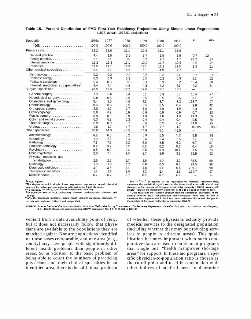
Ch. 2–Supply ● 3 1
Table 15.—Percent Distribution of FMG First-Year Residency Projections Using Simple Linear Regressions(1976 actual, 1977.81 projections)
Specialty 1976a 1977 1978 1979 1980 1981 Fb RZb
Total:. . . . . . . . . . . . . . . . . . . . . . . 100.0 100.0 100.0 100.0 100.0 100.0
Primary care . . . . . . . . . . . . . . . . . . . . . 33.2 31.6 32.1 32.6 33.1 33.6General practice. . . . . . . . . . . . . . . . 4.4 3.5 3.6 3.7 3.8 3.9 0.7 - .12Family practice. . . . . . . . . . . . . . . . . 3.1 3.1 3.5 3.9 4.3 4.7 27.2 .87Internal medicine. . . . . . . . . . . . . . . 13.2 13.3 13.1 12.9 12.7 12.5 2.0 .28Pediatrics . . . . . . . . . . . . . . . . . . . . . 12.5 11.7 11.9 12.1 12.3 12.5 1.3 .21
Other medical specialties . . . . . . . . . . 5.4 5.2 5.2 5.1 4.9 4.7 — —
Dermatology. . . . . . . . . . . . . . . . . . . 0.3 0.2 0.2 0.2 0.2 0.1 6.7 .57Pediatric allergy. . . . . . . . . . . . . . . . 0.3 0.3 0.3 0.3 0.3 0.3 0.1 .02Pediatric cardiology. . . . . . . . . . . . . 0.4 0.3 0.3 0.3 0.3 0.2 10.4 .68Internal medicine subspecialtiesd . 4.4 4.4 4.4 4.3 4.2 4.1 2.2 .31
Surgical specialties. . . . . . . . . . . . . . . 20.5 19.0 18.2 17.6 17.0 16.2 — —
General surgery. . . . . . . . . . . . . . . . 7.0 6.6 6.4 6.1 5.9 5.7 16.4 .77Neurological surgery. . . . . . . . . . . . 0.8 0.5 0.5 0.5 0.5 0.5 0.1 .02Obstectrics and gynecology . . . . . . 5.4 5.0 4.6 4.1 3.7 3.3 138.7 .97Ophthalmology. . . . . . . . . . . . . . . . . 0.5 0.6 0.5 0.5 0.5 0.4 3.6 .42Orthopedic surgery . . . . . . . . . . . . . 2.0 1.7 1.7 1.8 1.9 1.9 2.3 .31Otolaryngology. . . . . . . . . . . . . . . . . 0.9 0.9 0.9 0.9 0.9 0.9 0.7 .13Plastic surgery . . . . . . . . . . . . . . . . . 0.8 0.9 0.9 1.0 1.0 1.0 41.3 .89Colon and rectal surgery . . . . . . . . . 0.3 0.3 0.3 0.4 0.4 0.4 9.5 .65Thoracic surgery . . . . . . . . . . . . . . . 0.9 0.8 0.7 0.6 0.5 0.4 14.9 .75Urology . . . . . . . . . . . . . . . . . . . . . . . 1.8 1.7 1.7 1.7 1.7 1.7 .00005 .00001
Other specialties . . . . . . . . . . . . . . . . . 40.9 44.3 44.5 44.8 45.1 45.5 — —
Anesthesiology . . . . . . . . . . . . . . . . 6.2 6.6 6.2 5.9 5.5 5.2 6.5 .56Neurology . . . . . . . . . . . . . . . . . . . . . 1.9 2.3 2.3 2.4 2.4 2.5 2.7 .35Pathology . . . . . . . . . . . . . . . . . . . . . 7.1 7.5 7.2 6.8 6.5 6.2 6.7 .57Forensic pathology . . . . . . . . . . . . . 0.2 0.2 0.2 0.2 0.2 0.2 0.4 .10Psychiatry . . . . . . . . . . . . . . . . . . . . . 8.5 9.2 9.4 9.6 9.9 10.1 1.5 .23Child psychiatry. . . . . . . . . . . . . . . . 2.0 2.3 2.5 2.7 2.9 3.1 55.5 .92Physical medicine and
rehabilitation . . . . . . . . . . . . . . . . 2.5 2.5 2.7 2.9 3.0 3.2 38.5 .89Radiology . . . . . . . . . . . . . . . . . . . . . 1.3 1.6 1.2 0.8 0.5 0.1 29.5 .86Diagnostic radiology . . . . . . . . . . . . 3.0 3.6 4.1 4.6 5.1 5.6 239.7 .98Therapeutic radiology . . . . . . . . . . . 1.5 1.8 2.0 2.2 2.4 2.6 154.7 .97Miscellaneous. . . . . . . . . . . . . . . . . 6.7 6.7 6.7 6.7 6.7 6.7 – –
aActual figures. The “F Test:’%he degree to which simple Iinear regression represents actual historical
as applied to the regression on historical residency data,measures the statistical significanceof the linear trend asan estimateof past
trends intheindiwdual specialties is reflected in the Fand Revalues. changes in the number of first-year residentsby specialty 1966.76, Valuesof FcFlguresmay not add tototal dueto independent rounding. greaterthan 6,6 are statistically significant at the95-percent confidence level,dlncludes gastroenterology, pulmonary disease, cardiovascular disease, and Ry, the squareof the Pearson product-moment correlation coefficient, isfre-
allergy. quently referred teas’’TheCorrelation index’’Onascale from zero to one, (telncludes aerospace medicine, public health, general preventive medicine, oc- measures the degreeto which the Iinear trend estimates the actual changes in
cupatlonal medicine, “other,” and unspecified, the number of first-year residents, by specialty, 1968-76.
SOURCE: Irrtermr Report of the Graduate Medical Education Natfona/ Adwsory Corrrrrr/ttee to the Secrefary, Departrnerrt of ffea/tfr, Educa(/err, and We/fare, Washington,D.C : Health Resources Administration, DHEW publication No. (HRA) 79-633, p 129-130
venient from a data availability point of view,but it does not necessarily follow that physi-cians are available to the populations they arematched against. Nor are populations identifiedon these bases comparable, and one area (e. g.,county) may have people with significantly dif-ferent health problems than people in otherareas. So in addition to the basic problem ofbeing able to count the numbers of practicingphysicians and their clinical specialties in anidentified area, there is the additional problem
of whether these physicians actually providemedical services to the designated population(including whether they may be providing serv-ices to people in adjacent areas). This qual-ification becomes important when such com-parative data are used to implement programsthat single out “health manpower shortageareas” for support. In these aid programs, a spe-cific physician-to-population ratio is chosen asthe cutoff point and used in conjunction withother indices of medical need to determine
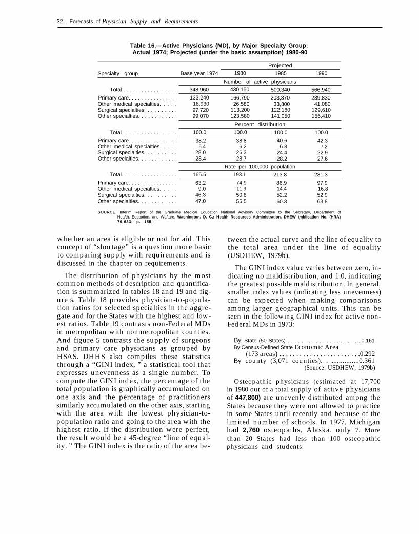
32 . Forecasts of Physician Supply and Requirements
Table 16.—Active Physicians (MD), by Major Specialty Group:Actual 1974; Projected (under the basic assumption) 1980-90
Projected
Specialty group Base year 1974 1980 1985 1990
Number of active physicians
Total . . . . . . . . . . . . . . . . . . 348,960 430,150 500,340 566,940
Primary care. . . . . . . . . . . . . . . . 133,240 166,790 203,370 239,830Other medical specialties. . . . . 18,930 26,580 33,800 41,080Surgical specialties. . . . . . . . . . 97,720 113,200 122,160 129,610Other specialties. . . . . . . . . . . . 99,070 123,580 141,050 156,410
Percent distribution
Total . . . . . . . . . . . . . . . . . . 100.0 100.0 100.0 100.0
Primary care. . . . . . . . . . . . . . . . 38.2 38.8 40.6 42.3Other medical specialties. . . . . 5.4 6.2 6.8 7.2Surgical specialties. . . . . . . . . . 28.0 26.3 24.4 22.9Other specialties. . . . . . . . . . . . 28.4 28.7 28.2 27,6
Rate per 100,000 population
Total . . . . . . . . . . . . . . . . . . 165.5 193.1 213.8 231.3
Primary care. . . . . . . . . . . . . . . . 63.2 74.9 86.9 97.9Other medical specialties. . . . . 9.0 11.9 14.4 16.8Surgical specialties. . . . . . . . . . 46.3 50.8 52.2 52.9Other specialties. . . . . . . . . . . . 47.0 55.5 60.3 63.8
SOURCE: Interim Report of the Graduate Medical Education National Advisory Committee to the Secretary, Department ofHea/th. Education. and We/tare. Washington. D. C,: Health Resources Administration. DHEW tmblicatlon No, (HRA). . . ,79-633; p. 155.
“ .
whether an area is eligible or not for aid. Thisconcept of “shortage” is a question more basicto comparing supply with requirements and isdiscussed in the chapter on requirements.
The distribution of physicians by the mostcommon methods of description and quantifica-tion is summarized in tables 18 and 19 and fig-ure S. Table 18 provides physician-to-popula-tion ratios for selected specialties in the aggre-gate and for the States with the highest and low-est ratios. Table 19 contrasts non-Federal MDsin metropolitan with nonmetropolitan counties.And figure 5 contrasts the supply of surgeonsand primary care physicians as grouped byHSAS. DHHS also compiles these statisticsthrough a “GINI index, ” a statistical tool thatexpresses unevenness as a single number. Tocompute the GINI index, the percentage of thetotal population is graphically accumulated onone axis and the percentage of practitionerssimilarly accumulated on the other axis, startingwith the area with the lowest physician-to-population ratio and going to the area with thehighest ratio. If the distribution were perfect,the result would be a 45-degree “line of equal-ity. ” The GINI index is the ratio of the area be-
tween the actual curve and the line of equality tothe total area under the line of equality(USDHEW, 1979b).
The GINI index value varies between zero, in-dicating no maldistribution, and 1.0, indicatingthe greatest possible maldistribution. In general,smaller index values (indicating less unevenness)can be expected when making comparisonsamong larger geographical units. This can beseen in the following GINI index for active non-Federal MDs in 1973:
By State (50 States) . . . . . . . . . . . . . . . . . . . . ..0.161By Census-Defined State Economic Area
(173 areas) ... , . . . . . . . . . . . . . . . . . . . . .0.292By county (3,071 counties). . ...............0.361
(Source: USDHEW, 1979b)
Osteopathic physicians (estimated at 17,700in 1980 out of a total supply of active physiciansof 447,800) are unevenly distributed among theStates because they were not allowed to practicein some States until recently and because of thelimited number of schools. In 1977, Michiganhad 2,760 osteopaths, Alaska, only 7. Morethan 20 States had less than 100 osteopathicphysicians and students.
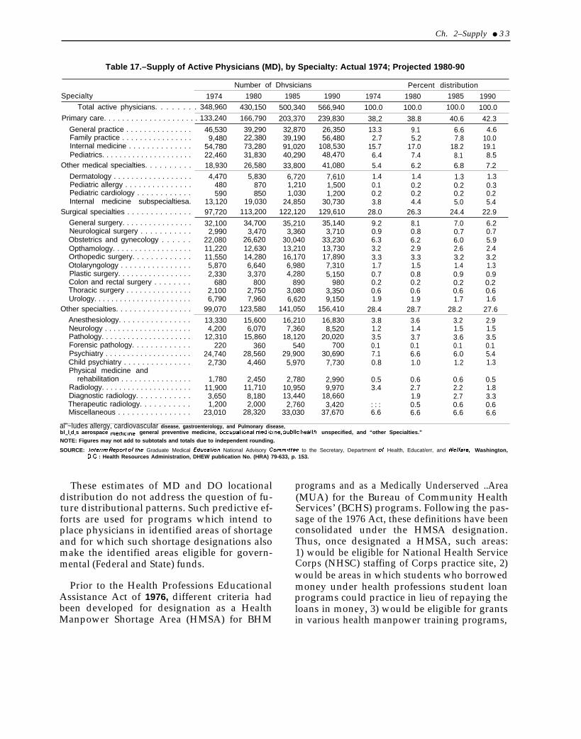
Ch. 2–Supply ● 3 3
Table 17.–Supply of Active Physicians (MD), by Specialty: Actual 1974; Projected 1980-90
Number of Dhvsicians Percent distributionSpecialty 1974 1980 1985 1990 1974 1980 1985 1990
Total active physicians. . . . . . . . 348,960 430,150 500,340 566,940 100.0 100.0 100.0 100.0Primary care. . . . . . . . . . . . . . . . . . . . . 133,240 166,790 203,370 239,830 38,2 38.8 40.6 42.3
General practice . . . . . . . . . . . . . . . 46,530 39,290 32,870 26,350 13.3 9.1 6.6 4.6Family practice . . . . . . . . . . . . . . . . 9,480 22,380 39,190 56,480 2.7 5.2 7.8 10.0Internal medicine . . . . . . . . . . . . . . 54,780 73,280 91,020 108,530 15.7 17.0 18.2 19.1Pediatrics. . . . . . . . . . . . . . . . . . . . . 22,460 31,830 40,290 48,470 6.4 7.4 8.1 8.5
Other medical specialties. . . . . . . . . . 18,930 26,580 33,800 41,080 5.4 6.2 6.8 7.2Dermatology . . . . . . . . . . . . . . . . . . 4,470 5,830 6,720 7,610 1.4 1.4 1.3 1.3Pediatric allergy . . . . . . . . . . . . . . . 480 870 1,210 1,500 0.1 0.2 0.2 0.3Pediatric cardiology . . . . . . . . . . . . 590 850 1,030 1,200 0.2 0.2 0.2 0.2Internal medicine subspecialtiesa. 13,120 19,030 24,850 30,730 3.8 4.4 5.0 5.4
Surgical specialties . . . . . . . . . . . . . . 97,720 113,200 122,120 129,610 28.0 26.3 24.4 22.9General surgery. . . . . . . . . . . . . . . . 32,100 34,700 35,210 35,140 9.2 8.1 7.0 6.2Neurological surgery . . . . . . . . . . . 2,990 3,470 3,360 3,710 0.9 0.8 0.7 0.7Obstetrics and gynecology . . . . . . 22,080 26,620 30,040 33,230 6.3 6.2 6.0 5.9Opthamology. . . . . . . . . . . . . . . . . . 11,220 12,630 13,210 13,730 3.2 2.9 2.6 2.4Orthopedic surgery. . . . . . . . . . . . . 11,550 14,280 16,170 17,890 3.3 3.3 3.2 3.2Otolaryngology . . . . . . . . . . . . . . . . 5,870 6,640 6,980 7,310 1.7 1.5 1.4 1.3Plastic surgery. . . . . . . . . . . . . . . . . 2,330 3,370 4,280 5,150 0.7 0.8 0.9 0.9Colon and rectal surgery . . . . . . . . 680 800 890 980 0.2 0.2 0.2 0.2Thoracic surgery . . . . . . . . . . . . . . . 2,100 2,750 3,080 3,350 0.6 0.6 0.6 0.6Urology. . . . . . . . . . . . . . . . . . . . . . . 6,790 7,960 6,620 9,150 1.9 1.9 1.7 1.6
Other specialties. . . . . . . . . . . . . . . . . 99,070 123,580 141,050 156,410 28.4 28.7 28.2 27.6Anesthesiology. . . . . . . . . . . . . . . . 13,330 15,600 16,210 16,830 3.8 3.6 3.2 2.9Neurology . . . . . . . . . . . . . . . . . . . . 4,200 6,070 7,360 8,520 1.2 1.4 1.5 1.5Pathology. . . . . . . . . . . . . . . . . . . . . 12,310 15,860 18,120 20,020 3.5 3.7 3.6 3.5Forensic pathology. . . . . . . . . . . . . 220 360 540 700 0.1 0.1 0.1 0.1Psychiatry . . . . . . . . . . . . . . . . . . . . 24,740 28,560 29,900 30,690 7.1 6.6 6.0 5.4Child psychiatry . . . . . . . . . . . . . . . 2,730 4,460 5,970 7,730 0.8 1.0 1.2 1.3Physical medicine and
rehabilitation . . . . . . . . . . . . . . . . 1,780 2,450 2,780 2,990 0.5 0.6 0.6 0.5Radiology. . . . . . . . . . . . . . . . . . . . . 11,900 11,710 10,950 9,970 3.4 2.7 2.2 1.8Diagnostic radiology. . . . . . . . . . . . 3,650 8,180 13,440 18,660 1.9 2.7 3.3Therapeutic radiology. . . . . . . . . . . 1,200 2,000 2,760 3,420 : : : 0.5 0.6 0.6Miscellaneous . . . . . . . . . . . . . . . . 23,010 28,320 33,030 37,670 6.6 6.6 6.6 6.6
al”~ludes allergy, cardiovascular disease, gastroenterology, and Pulmonary disease,blncludes aerospace medlclne, general preventive medicine, occupational medicine, public health, unspecified, and “other Specialties.”
NOTE: Figures may not add to subtotals and totals due to independent rounding.
SOURCE: Intermr Report of the Graduate Medical Educat/on National Advisory Cornffr/ttee to the Secretary, Department of Health, Educat/err, and Welfare, Washington,D.C : Health Resources Administration, DHEW publication No. (HRA) 79-633, p. 153.
These estimates of MD and DO locationaldistribution do not address the question of fu-ture distributional patterns. Such predictive ef-forts are used for programs which intend toplace physicians in identified areas of shortageand for which such shortage designations alsomake the identified areas eligible for govern-mental (Federal and State) funds.
Prior to the Health Professions EducationalAssistance Act of 1976, different criteria hadbeen developed for designation as a HealthManpower Shortage Area (HMSA) for BHM
programs and as a Medically Underserved ..Area(MUA) for the Bureau of Community HealthServices’ (BCHS) programs. Following the pas-sage of the 1976 Act, these definitions have beenconsolidated under the HMSA designation.Thus, once designated a HMSA, such areas:1) would be eligible for National Health ServiceCorps (NHSC) staffing of Corps practice site, 2)would be areas in which students who borrowedmoney under health professions student loanprograms could practice in lieu of repaying theloans in money, 3) would be eligible for grantsin various health manpower training programs,
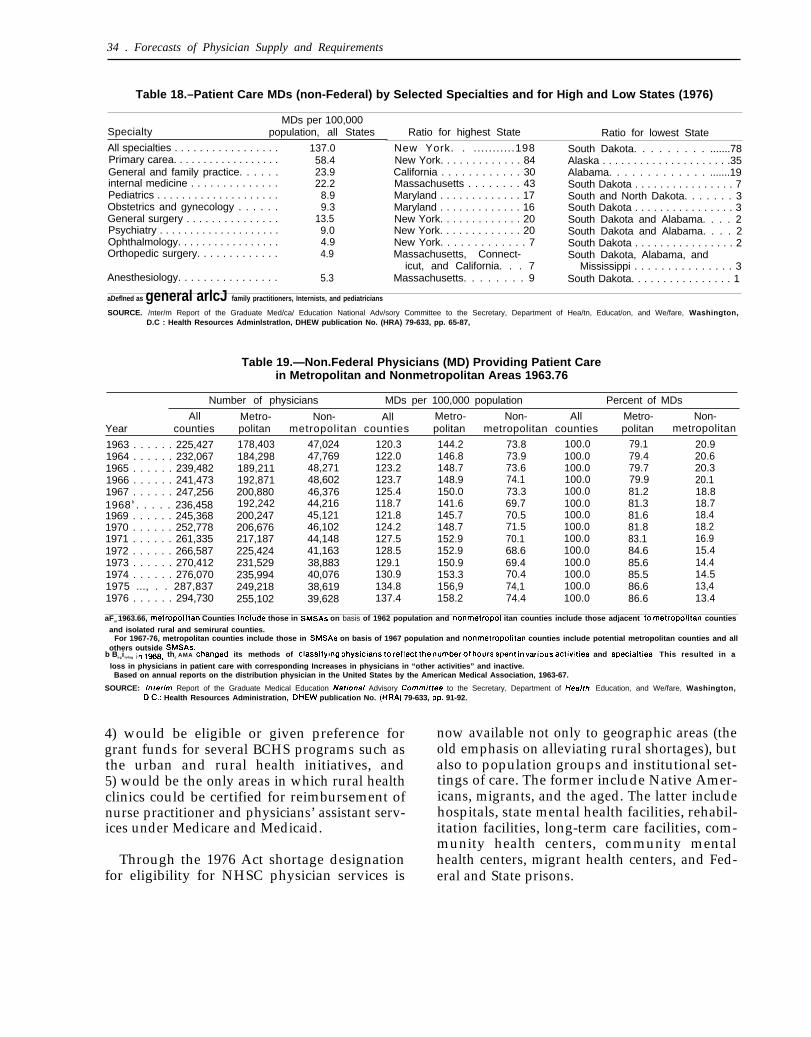
—
34 . Forecasts of Physician Supply and Requirements
Table 18.–Patient Care MDs (non-Federal) by Selected Specialties and for High and Low States (1976)
MDs per 100,000Specialty population, all States
All specialties . . . . . . . . . . . . . . . . .Primary carea. . . . . . . . . . . . . . . . . .General and family practice. . . . . .internal medicine . . . . . . . . . . . . . .Pediatrics . . . . . . . . . . . . . . . . . . . .Obstetrics and gynecology . . . . . .General surgery . . . . . . . . . . . . . . .Psychiatry . . . . . . . . . . . . . . . . . . . .Ophthalmology. . . . . . . . . . . . . . . . .Orthopedic surgery. . . . . . . . . . . . .
137.058.423.922.2
8.99.3
13.59.04.94.9
Anesthesiology. . . . . . . . . . . . . . . . 5.3
Ratio for highest State Ratio for lowest State
New York. . ...........198 South Dakota. . . . . . . . . .......78New York. . . . . . . . . . . . . 84 Alaska . . . . . . . . . . . . . . . . . . . . .35California . . . . . . . . . . . . 30 Alabama. . . . . . . . . . . . . .......19Massachusetts . . . . . . . . 43 South Dakota . . . . . . . . . . . . . . . . 7Maryland . . . . . . . . . . . . . 17 South and North Dakota. . . . . . . 3Maryland . . . . . . . . . . . . . 16 South Dakota . . . . . . . . . . . . . . . . 3New York. . . . . . . . . . . . . 20 South Dakota and Alabama. . . . 2New York. . . . . . . . . . . . . 20 South Dakota and Alabama. . . . 2New York. . . . . . . . . . . . . 7 South Dakota . . . . . . . . . . . . . . . . 2Massachusetts, Connect- South Dakota, Alabama, and
icut, and California. . . 7 Mississippi . . . . . . . . . . . . . . . 3Massachusetts. . . . . . . . 9 South Dakota. . . . . . . . . . . . . . . . 1
aDeflned as general arlcJ family practitioners, Internists, and pediatricians
SOURCE. /nter/m Report of the Graduate Med/ca/ Education National Adv/sory Committee to the Secretary, Department of Hea/tn, Educat/on, and We/fare, Washington,D.C : Health Resources Adminlstratlon, DHEW publication No. (HRA) 79-633, pp. 65-87,
Table 19.—Non.Federal Physicians (MD) Providing Patient Carein Metropolitan and Nonmetropolitan Areas 1963.76
Number of physicians MDs per 100,000 population Percent of MDs
All Metro- Non- All Metro- Non- All Metro- Non-Year counties politan metropolitan counties politan metropolitan counties politan metropolitan
1963 . . . . . . 225,427 178,403 47,024 120.3 144.2 73.8 100.0 79.1 20.91964 . . . . . . 232,067 184,298 47,769 122.0 146.8 73.9 100.0 79.4 20.61965 . . . . . . 239,482 189,211 48,271 123.2 148.7 73.6 100.0 79.7 20.31966 . . . . . . 241,473 192,871 48,602 123.7 148.9 74.1 100.0 79.9 20.11967 . . . . . . 247,256 200,8801968 b . . . . . 236,458
46,376 125.4 150.0 73.3 100.0 81.2 18.8192,242 44,216 118.7 141.6 69.7 100.0 81.3 18.7
1969 . . . . . . 245,368 200,247 45,121 121.8 145.7 70.5 100.0 81.6 18.41970 . . . . . . 252,778 206,676 46,102 124.2 148.7 71.5 100.0 81.8 18.21971 . . . . . . 261,335 217,187 44,148 127.5 152.9 70.1 100.0 83.1 16.91972 . . . . . . 266,587 225,424 41,163 128.5 152.9 68.6 100.0 84.6 15.41973 . . . . . . 270,412 231,529 38,883 129.1 150.9 69.4 100.0 85.6 14.41974 . . . . . . 276,070 235,994 40,076 130.9 153.3 70.4 100.0 85.5 14.51975 ..., . . 287,837 249,218 38,619 134.8 156,9 74,1 100.0 86.6 13,41976 . . . . . . 294,730 255,102 39,628 137.4 158.2 74.4 100.0 86.6 13.4
aFor 1963.66, metropoi itan Counties include those in SMSAS on basis of 1962 population and nonmetropol itan counties include those adjacent to metrOPOlitan counties
and isolated rural and semirural counties.For 1967-76, metropolitan counties include those in SMSAS on basis of 1967 population and nonmetropolitan counties include potential metropolitan counties and all
others outside SMSAS.b Beginnlng in 1968, the AMA changed its methods of Classlfylng physicians to reflect the number of hours spent in various actiwties and .Specialties. This resulted in a
loss in physicians in patient care with corresponding Increases in physicians in “other activities” and inactive.Based on annual reports on the distribution physician in the United States by the American Medical Association, 1963-67.
SOURCE: /nterim Report of the Graduate Medical Education Naoonal Advisory Comm/ttee to the Secretary, Department of Hea/th, Education, and We/fare, Washington,DC.: Health Resources Administration, DHEW publication No. (HRA) 79-633, pp. 91-92.
4) would be eligible or given preference forgrant funds for several BCHS programs such asthe urban and rural health initiatives, and5) would be the only areas in which rural healthclinics could be certified for reimbursement ofnurse practitioner and physicians’ assistant serv-ices under Medicare and Medicaid.
Through the 1976 Act shortage designationfor eligibility for NHSC physician services is
now available not only to geographic areas (theold emphasis on alleviating rural shortages), butalso to population groups and institutional set-tings of care. The former include Native Amer-icans, migrants, and the aged. The latter includehospitals, state mental health facilities, rehabil-itation facilities, long-term care facilities, com-munity health centers, community mentalhealth centers, migrant health centers, and Fed-eral and State prisons.
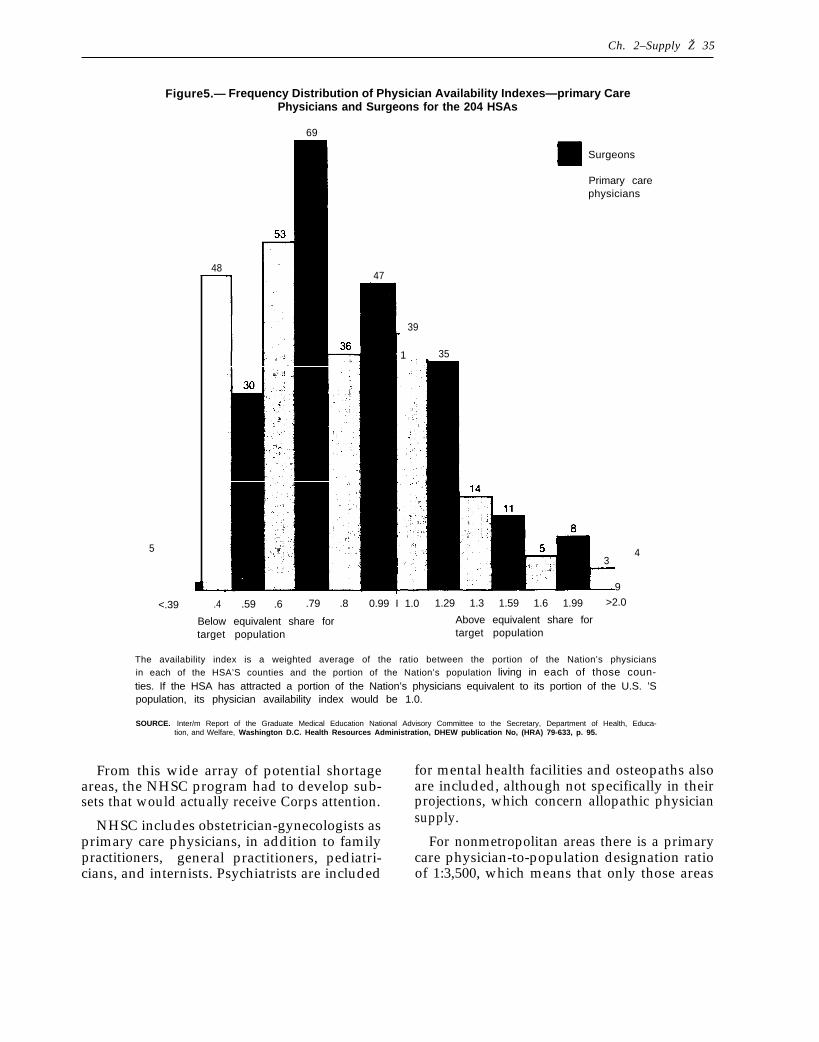
Ch. 2–Supply Ž 35
Figure5.— Frequency Distribution of Physician Availability Indexes—primary Care.Physicians and Surgeons for the 204 HSAs
69
5
<.39
48
Surgeons
Primary carephysicians
47
39
1 35
34
9
.4 .59 .6 .79 .8 0.99 I 1.0 1.29 1.3 1.59 1.6 1.99 >2.0
Below equivalent share for Above equivalent share fortarget population target population
The availability index is a weighted average of the ratio between the portion of the Nation’s physiciansin each of the HSA’S counties and the portion of the Nation’s population living in each of those coun-ties. If the HSA has attracted a portion of the Nation’s physicians equivalent to its portion of the U.S. ’Spopulation, its physician availability index would be 1.0.
SOURCE. Inter/m Report of the Graduate Medical Education National Advisory Committee to the Secretary, Department of Health, Educa-tion, and Welfare, Washington D.C. Health Resources Administration, DHEW publication No, (HRA) 79-633, p. 95.
From this wide array of potential shortage for mental health facilities and osteopaths alsoareas, the NHSC program had to develop sub- are included, although not specifically in theirsets that would actually receive Corps attention. projections, which concern allopathic physician
NHSC includes obstetrician-gynecologists as supply.
primary care physicians, in addition to family For nonmetropolitan areas there is a primarypractitioners, general practitioners, pediatri- care physician-to-population designation ratiocians, and internists. Psychiatrists are included of 1:3,500, which means that only those areas
36 ● Forecasts of Physician Supply and Requirements
with that ratio or higher (fewer physicians)would be eligible for Corps staffing. The targetratio is 1:2,000. Once designated and selectedfor Corps staffing, Corps physicians would beprovided until a ratio of 1:2,000 was achieved(USDHEW, 1978a).
As part of the process of planning for howmuch effort is needed in specific practice set-tings, estimates must be made of the numbersand types of physicians who will settle in theseareas voluntarily. DHHS, through the joint ef-forts of its BHM of the Health Resources Ad-ministration and the Office of Planning, Evalua-
. tion, and Legislation of the Health Services Ad-ministration, has developed a computerizedmodel to project the number and distribution ofactive, non-Federal, office-based patient carephysicians in the so States and all counties from1972 through 1990.
As the Health Professions Educational Assist-ance Act of 1976 enlarged the definition ofHMSAS, separate estimates are made for: 1)rural counties, 2) urban areas, 3) Federal andState prisons, 4) State mental hospitals andcommunity mental health centers, and 5) the In-dian Health Service. The computerized model isused to project future supply in rural counties,but it cannot be used to project supply in theother categories. Hence, other methods must beused for these other categories. For prisons,mental health facilities, and the Indian HealthService, the sponsoring agencies have providedestimates of both supply and requirements. Es-sentially, these agencies forecast a steady statesupply (USDHEW, 1978a).
The NHSC task force’s estimates of the sup-ply of primary care physicians in rural and ur-ban areas are summarized below.
Rural areas. —The projections are based on:1) existing supply (DOS and MDs, domestic andforeign graduates); 2) anticipated deaths, retire-ments, and relocation of existing physicians; 3)anticipated graduations, specialty choices, andpractice locations; and 4) anticipated popula-tion growth. Beginning with 1972 as the baseyear, total physician and primary care and non-primary care physician-to-population ratios areprojected for each county (urban as well as
rural) for each year. The method is thus similarto aggregate and specialty supply, with theadded factor of accounting for where physicianslocate.
Counties are assumed to maintain populationas fixed proportions (derived from 1972 data) oftheir respective State populations.
Starting with the 1972 active, non-Federal,office-based, patient-care physicians in eachcounty, year-by-year reductions from deathsand retirement are calculated.
The number of new physicians expected toenter practice is estimated by the method de-scribed earlier for aggregate supply. These num-bers are summarized in table 20.
Total new physicians entering practice eachyear are reduced for: 1) Federal employment, 2)nonpatient care activities, and 3) practices inareas other than the so States.
The physician distribution among the Statesfor 1973-87 (since updated to the 1990’s) is basedon the historical pattern of distribution for grad-uates from 1965 to 1969, modified for percentchanges in State populations projected for 1972to 1987.
The percent of physicians entering practicefrom 1973 to 1987 as primary care specialists is
Table 20.—New Physicians EnteringPractice, 1973-87
Year USMG FMG DO
1973 . . . . . . . . . . . . . . 8,367 3,665 4721974 . . . . . . . . . . . . . . 8,974 5,081 4851975 . . . . . . . . . . . . . . 9,551 5,202 6491976 . . . . . . . . . . . . . . 10,391 2,709 5871977 . . . . . . . . . . . . . . 11,613 3,799 7021978 . . . . . . . . . . . . . . 12,714 5,265 8091979 . . . . . . . . . . . . . . 13,561 3,517 9081980 . . . . . . . . . . . . . . 13,607 3,895 9641981 . . . . . . . . . . . . . . 14,598 1,903 9961982 . . . . . . . . . . . . . . 15,048 2,187 1,0291983 . . . . . . . . . . . . . . 15,346 1,849 1,2081984 . . . . . . . . . . . . . . 15,789 2,372 1,3081985 . . . . . . . . . . . . . . 16,354 2,034 1,3771986 . . . . . . . . . . . . . . 16,956 2,246 1,4581987 . . . . . . . . . . . . . . 17,241 1,908 1,496
SOURCE: Memorandum from the Chairmm, NHSC Needs Task Force A, to theDirector, Bureau of Community Health Services, Health Services Ad-ministration; the Deputy Director, Bureau of Health Manpower,Health Resources Administration; and the Chairman, NHSC NeedsTask Force, Washington, D. C,, May 26,1978.
Ch. 2–Supply Ž 37
projected to increase to the proportions listed intable 21. This should be distinguished from thepercent of the total physician supply that is pro-jected to be in primary care (tables 16 and 17).
Physicians are projected to enter practice incounty classes in the percentages summarized intable 22.
Newly entering physicians are allocated to in-dividual counties by specialty according to the1974 observed pattern of 30-to 44-year-old phy-sicians of the same specialty. This new supply isadded to the existing supply, modified yearlyfor attrition from deaths and retirements.
Table 21 .—Percent of New PhysiciansExpected To Enter Primary Care
Percent inYear primary care
1973 . . . . . . . . . . . . . . . . . . . . . . . . . . . . . . . . . 25.21974 . . . . . . . . . . . . . . . . . . . . . . . . . . . . . . . . . 26.41975 . . . . . . . . . . . . . . . . . . . . . . . . . . . . . . . . . 28.11976 . . . . . . . . . . . . . . . . . . . . . . . . . . . . . . . . . 33.51977 . . . . . . . . . . . . . . . . . . . . . . . . . . . . . . . . . 37.51978 . . . . . . . . . . . . . . . . . . . . . . . . . . . . . . . . . 43.21979 . . . . . . . . . . . . . . . . . . . . . . . . . . . . . . . . . 43.81980 . . . . . . . . . . . . . . . . . . . . . . . . . . . . . . . . . 46.01981 . . . . . . . . . . . . . . . . . . . . . . . . . . . . . . . . . 48.11982 . . . . . . . . . . . . . . . . . . . . . . . . . . . . . . . . . 50.21983 . . . . . . . . . . . . . . . . . . . . . . . . . . . . . . . . . 52.21984-87. . . . . . . . . . . . . . . . . . . . . . . . . . . . . . . 52.2
SOURCE: Memorandum from the chairman, NHSC Needs Task Force A,to theDirector, Bureau of Community Health services, Health Services Ad-ministration; the Deputy Director, Bureau of Health Manpower,Health Resources Administration; and the Chairman, NHSC NeedsTask Force, Washington, D.C., May26,1978.
Urban area. —Predicting the future supply ofphysicians for urban areas in order to assess theneed for additional physicians is not computedon a county basis. If measured by county, thenumber of primary care physicians is usuallyadequate, so the needs in urban areas are meas-ured by the needs of certain population groupswhich have financial and sociocultural barriersto access instead of the geographic barriers ofrural areas, for which physician-to-populationratios serve as substantial proxy measures.Thus, an estimate of the number of physiciansrequired to meet the needs of metropolitan low-income areas as defined by the Bureau of theCensus is used.
Such identified low-income area populationsdeclined from 17,936,000 in 1974 to 16,554,000in 1976, or a decline of 3.8 percent per year. Butthe task force concluded that the decrease is notexpected to continue indefinitely and that thereis a current trend for physicians in central citiesto move to the suburbs. It therefore assumedthat the decrease in low-income population willbe offset or more than offset by the emigrationof physicians from the inner city. In otherwords, present supply as expressed in physician-to-population ratios also predicts what the fu-ture supply will be. This average is 13.3 full-time-equivalent primary care physicians per100,000population o
Parenthetically, it was determined that 42.3primary care physicians per 100,000 population
Table 22.—Projected County Classes of Newly Practicing Physicians
MD
County classa Family practice Primary careb Non primary care DO
1 2.7 0.2 0.1 3.0. . . . . . . . . . . . . . .2 7.5 2.0 0.5 6.7. . . . . . . . . . . . . . .3 10.6 5.1 1.6 6.4. . . . . . . . . . . . . . .4 9.4 6.9 3.7 5.2. . . . . . . . . . . . . . .5 2.3 2.2 1.2 2.2. . . . . . . . . . . . . . .6 26.8 19.5 24.6 17.6. . . . . . . . . . . . . . .
13.2 12.8 13.1 13.97:: : : : : : : : : : : : : : : 21.9 35.5 37.0 40.19 . . . . . . . . . . . . . . . 5.6 15.0 18.2 4.9
100.0 100.0 100.0 100.0
aAMA demographic county classification (1-4 = rural; 5-9 = urban).bExcluding family pra~tlce, This definition of ‘Jprima~ care” includes obstetrics-gynecology, in addition tO Qenerd praCtlCe,
family practice, internal medicine, and pediatrics.
SOURCE: Memorandum from the Chairman, NHSC Needs Task Force A, to the Director, Bureau of Community Health Serv-ices, Health Services Administration; the Deputy Director, Bureau of Health Manpower, Health Resources Admin-istration; and the Chairman, NHSC Needs Task Force, Washington, DC., May 26,1978.
38 ● Forecasts of Physician Supply and Requirements
(a staffing ratio of 1:2,000) would be needed inthese low-income areas and that the 13.3 num-ber meant that 31.4 percent of need was alreadymet. The analysis then goes on to say that sepa-rate analyses of the underserved population’s“usual source of care” resulted in the figures intable 23 and confirmed the 31.4-percent figure.
The analysis then goes on to equate the sumof care from “hospital, “ “neighborhood healthcenter, ” and “none” with unmet need of 62.6percent of the population and goes on to esti-mate additional physicians needed on this basis.Yet only 8.6 percent of the 62.6 percent receivedno care. Hospital care does not represent “un-met need” but involves the question of what isappropriate care. And since this analysis wasmade to estimate the number of NHSC physi-cians that might be placed in these areas, identi-
SUMMARY
Comparing the methods for estimating supplywith those used for estimating requirements, wewould expect more certainty in the supply pro-jections. Yet the foregoing description of supplyprojections shows that there are many weak-nesses in the data bases, some questionable as-sumptions underlying the projections, differentinterpretations given to some commonly usedterminologies such as “primary care” and “full-time-equivalent, ” etc.
The description of how supply projections aremade can quickly become quite detailed. So letus summarize: 1) the components and primaryassumptions of the supply estimates, and 2)some definitional problems that are linked tosubstantive issues and which are compoundedby weaknesses in the data.
Supply is the sum of practicing physiciansand additions of foreign and domestic medicaland osteopathic school graduates (there are noforeign additions to the osteopathic supply). At-trition from deaths and retirements for the prac-ticing physician component is estimated by age-specific rates. For specialty supply, the samedeath and retirement rates are applied to eachspecialty.
Table 23.—Usual Source of Carefor Urban Underserved Areas
PercentPrivate physicians. . . . . . . . . . . . . . . . . . . . . . 31.4Hospital (emergency room and
outpatient treatment). . . . . . . . . . . . . . . . . 31.3Neighborhood health center . . . . . . . . . . . . . 22.7None. . . . . . . . . . . . . . . . . . . . . . . . . . . . . . . . . 8.6Other . . . . . . . . . . . . . . . . . . . . . . . . . . . . . . . . 6.0
Total. . . . . . . . . . . . . . . . . . . . . . . . . . . . . . . 100.0
SOURCE: Memorandum from the Chairmanj NHSC Needs Task Force A, to theDirector, Bureau of community Health sewices, Healtfl se~ices A&ministration; the Deputy Director, Bureau of Health Manpower,Health Resources Administration; and the Chairman, NHSC NeedsTask Force, Washington, D. C., May 26,1978.
fying “neighborhood health center” care as “nocare” must mean that the presumption is thatsuch centers will be staffed only by NHSCphysicians in the future.
Additions to supply are the sum of foreignand domestic graduates. Estimates of first-yearenrollments and attrition prior to graduationare made to arrive at the number of domesticgraduates. The high, low, and basic first-yearenrollment estimates all assume full cavitationfunding by 1981, and 4, 7, or 10 new medicalschools after 1977-78. For FMG additions, theCanadian addition is currently estimated toequal losses from death, retirement, and emigra-tion. Estimates of the addition to supply fromother FMGs rely heavily on the presumed im-pact of the 1976 Act, which contained majorrestrictions on FMG immigration. It should benoted that the resulting total projections of sup-ply made before and after the 1976 Act have notvaried greatly (estimated at approximately600,000 in 1990). The component projections,however, have varied wiclely. In essence, pres-ent projections of domestic graduates are largerthan previous estimates, and present projectionsof FMG additions are less than prior estimates.In the current projections, the assumption of fullcavitation funding is not very realistic and tendsto increase the supply projections. On the otherhand, the additions from the FMG supply maybe too optimistic in terms of legislative impact
Ch. 2–Supply Ž 39
on decreasing this source of supply, particularlywith the large pool of U.S. citizens studyingmedicine abroad, for whom immigration re-strictions are not applicable, although they haveto pass a competency exam in order to practicemedicine in the United States.
Additions to specialty supply use projectionsof first-year residency trends to allocate foreignand domestic graduates among the specialties.The predictive power of first-year residencychoices is a problem because they may not re-flect ultimate specialty practices. This is particu-larly true for internal medicine, where at leastone-third of the first-year residency positions isused as a general medicine traineeship for physi-cians ultimately subspecializing or choosinganother specialty altogether. The trend inspecialty choice is determined by the trendreflected in the years 1968, 1970-74, and 1976,years in which major changes were occurring inthe structure of postgraduate medical trainingprograms. Statistical techniques also limit theapplicability of these trend years up to 1981, atwhich point the distribution is held constant forfuture years.
Methods for predicting the locational distri-bution of physicians are generally similar tothose for aggregate and specialty supply. Forrural areas, the active, non-Federal, office-basedphysician supply in each county is reduced fordeaths and retirements. The supply of new phy-sicians is allocated to individual counties by spe-cialty according to the 1974 observed patternsof 30- to 44-year-old physicians of the samespecialty (counties are allocated to nine classifi-cations from rural to urban). For urban (innercity) areas, physician supply is assumed to de-crease (no numbers given), reflecting continuedemigration to the suburbs. For prisons, mentalhealth ,services, and the Indian Health Service,future supply is generally assumed to hold cons-tant at its present rate.
In addition to absolute numbers, a relativestandard is used, the physician-to-populationratio, which is also commonly expressed as thenumber of physicians per 100,000 population;e.g., 1:1,000 or 100/100,000. This ratio is usedto provide a more complete quantification ofsupply; i.e., we need to know not only the
numbers of physicians in practice, but also thepopulations which they serve.
For aggregate and specialty supply, the Cen-sus Bureau’s Series II (or Series III, which pro-jects slower growth) estimates of population areused. As these reflect the 1970 Census, more ac-curate information will be available from theupcoming 1980 Census.
For locational distribution, the populationestimates try to be more specific, as supplyestimates are part of programmatic efforts to iden-tify HMSAS. For rural areas 1972 State popula-tion estimates are used, and counties are as-sumed to maintain fixed proportions of theirrespective State populations. For urban areas,the population is that identified by the Bureau ofthe Census as metropolitan low-income areas.Although these low-income populations havedeclined (17,936,000 in 1974 to 16,554,000 in1976, or a decline of 3.8 percent per year), thephysician-to-population ratio is assumed tohold constant in the future because of thepreviously mentioned expectation of continuedemigration of physicians out of the inner cities.
It should be obvious that supply, as refer-enced to population, depends not only on thephysician supply projections, but also on thepopulation projections. An example is the dis-tinction between projections of physician supplywhich include or exclude Federal physicians. Inprojecting supply for rural areas, table 19 esti-mated that there were 287,800 active non-Fed-eraI MDs in 1975. Table 9 estimates that therewere 363,400 active MDs (including Federal) in197s (377,500 minus 14,100 DOS). The 287,800figure was used to allocate physicians among allcounties. However, in subtracting the Federalphysician supply, no effort was made to de-crease the population by a proportional amount(these Federal physicians were active and pre-sumably providing patient care). In addition,1967 population estimates were used in table 19,whereas table 9 used population estimates thatincluded projections of population growth.
On the physician side of the ratio, table 9assumed that a portion of “not classified” MDswere active; whereas table 19 excluded this cate-gory from its count (approximately 30,000 phy-
40 ● Forecasts of Physician Supply and Requirements
sicians, or about 10 percent). In addition, table9 included DOS, table 19 did not.
So even though at first glance the differencesin the number of active physicians representedin tables 9 and 19 (377,500 v. 287,800) mightseem accounted for from the exclusion of Feder-al MDs, “not classified” physicians, and DOS intable 19, the method of quantifying the popula-tion also contributed to the different physician-to-population ratios (176.8/100,000 v. 134.8/100,000).
We have already seen that there are defini-tional problems associated with quantifyingphysician supply. These definitional problemswill take on even more significance once webegin to quantify requirements and try to matchthat with supply. Two basic problems are in-volved: 1) the amount of patient care that is at-tributed to the average physician, and 2) thetype of patient care provided.
The first problem is usually couched in termssuch as “productivity” or “full-time-equiv-alent, ” which attempt to provide a common ref-erence by which the number of physicians canbe equated to a certain volume of patient careservices. For example, physicians’ assistants inprisons were assumed to be equal to 0.5 physi-cians (USDHEW, 1978a). In this case, a physi-cian was equal to a full-time-equivalent (FTE),whatever the particular hours or number of pa-tients seen by prison physicians. Implicit in thisdefinition are assumptions on physician produc-tivity. Other uses of FTE are more explicit. In-diana uses a definition of a FTE primary carephysician as a general or family practitioner inthe age group 35 to 39, which has the highestoutput in terms of visits per year for thatspecialty (Hindle et al., 1978). A more commonmethod is to use average productivity figures byspecialty, either as measured by the average pa-tient care hours worked per week (hospital andambulatory care), the number of patients seenper week (usually expressed as the number ofambulatory visits), or both. And still anothermethod is to estimate what percent of time isspent on nonpatient care activities and subtractthat percentage from the total (aggregate or byspecialty) supply. These productivity or FTEestimates are crucial when comparing supply
with requirements, because they are the basicmethods underlying the comparison. Given thesame basic numbers of physician supply as pro-vided through “head counts” by the methodssummarized earlier, whether supply equals, fallsshort, or exceeds demand obviously depends onthe productivity assumptions applied to thephysician.
The definition of “primary care” involvesmore than the simple identification of whichspecialties “qualify” for that designation. Yet wehave already seen that what specialties count asprimary care is quite confusing. Even if we limitthe specialties to general practice, family prac-tice, general internal medicine, and generalpediatrics, there can be great variations in thequantification of primary care physicians, be-cause over 50 percent are in the internal med-icine category. Yet, at various times, some sub-specialties of internal medicine are included andsome are not. For example, table 13 excludesdermatology, gastroenterology, pulmonary dis-ease, cardiovascular disease, and allergy fromthe primary care internal medicine subspecial-ties, but includes allergy and immunology, dia-betes, endocrinology, geriatrics, hematology,immunology, infectious diseases, neoplastic dis-eases, nephrology, nutrition, oncology, andrheumatology.
The Institute of Medicine (1978) reviewed 38definitions of primary health care, and con-cluded that primary care cannot sufficiently bedefined by the location of care, by the provider’sdisciplinary training, or by the provision of aparticular set of services. It then goes on toelaborate on what it considers primary healthcare’s five essential attributes: 1) accessibility,2) comprehensiveness, 3) coordination, 4) con-tinuity, and 5) accountability.
In a study examining the general care contentof different specialty practices, the data was dis-aggregate into five components: 1) first en-counter, 2) episodic care, 3) principal care, 4)consultative care, and 5) specialized care (Aikenet al., 1979). Principal care was defined as:
There is evidence of continuity; the physicianreports having seen the patient before and con-siders him or her to be a regular patient. Com-
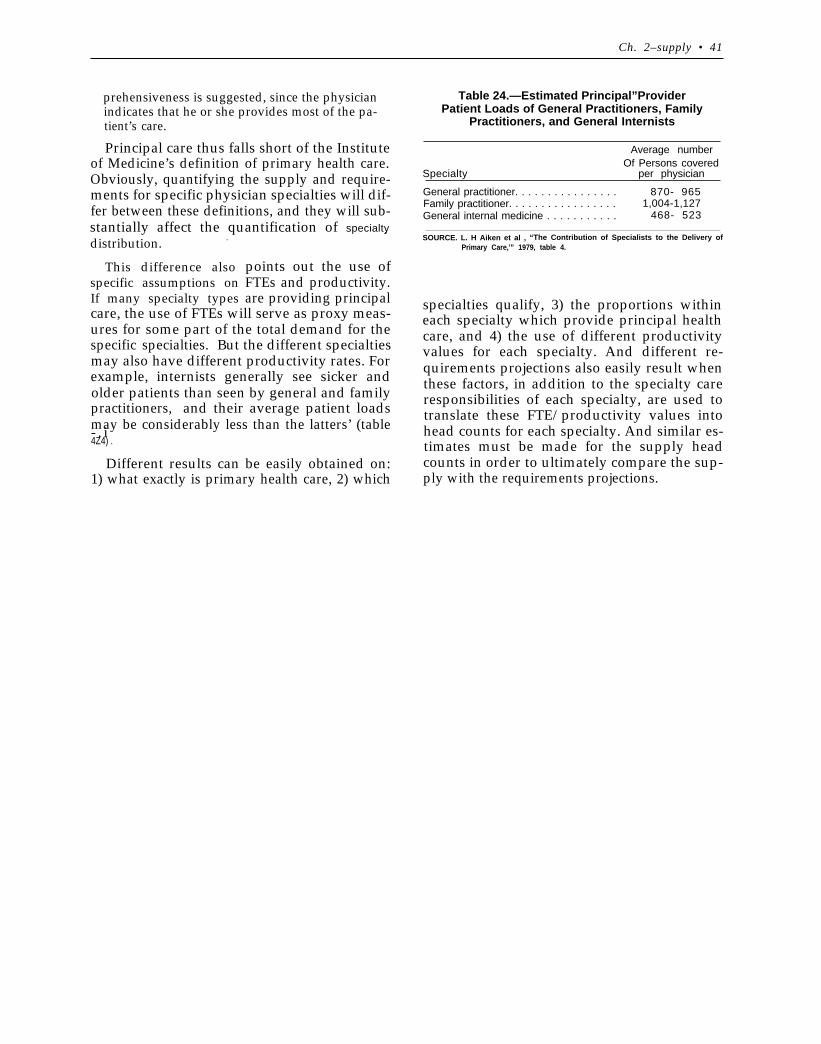
—
Ch. 2–supply • 41
prehensiveness is suggested, since the physicianindicates that he or she provides most of the pa-tient’s care.
Principal care thus falls short of the Instituteof Medicine’s definition of primary health care.Obviously, quantifying the supply and require-ments for specific physician specialties will dif-fer between these definitions, and they will sub-stantially affect the quantification of specialty
distribution. -
This difference alsospecific assumptions onIf many specialty types
Table 24.—Estimated Principal”ProviderPatient Loads of General Practitioners, Family
Practitioners, and General Internists
Average number
SpecialtyOf Persons covered
per physician
General practitioner. . . . . . . . . . . . . . . . 870- 965Family practitioner. . . . . . . . . . . . . . . . . 1,004-1,127General internal medicine . . . . . . . . . . . 468- 523
.SOURCE. L. H Aiken et al , “The Contribution of Specialists to the Delivery of
Primary Care,’” 1979, table 4.
points out the use ofFTEs and productivity.are providing principal
care, the use of FTEs will serve as proxy meas-ures for some part of the total demand for thespecific specialties. But the different specialtiesmay also have different productivity rates. Forexample, internists generally see sicker andolder patients than seen by general and familypractitioners, and their average patient loadsmay be considerably less than the latters’ (table- . i
specialties qualify, 3) the proportions withineach specialty which provide principal healthcare, and 4) the use of different productivityvalues for each specialty. And different re-quirements projections also easily result whenthese factors, in addition to the specialty careresponsibilities of each specialty, are used totranslate these FTE/productivity values intohead counts for each specialty. And similar es-
4Z4) . timates must be made for the supply headDifferent results can be easily obtained on: counts in order to ultimately compare the sup-
1) what exactly is primary health care, 2) which ply with the requirements projections.

3 .
Requirements
3.Requirements
INTRODUCTION
Faced with what seemed to be a straightfor-ward question on what our country’s physiciansupply is and will be, we have found that supplyprojections are not definitive and need to berevised periodically. And in somewhat circularfashion, supply projections can be substantiallydependent on deliberate Federal actions at thesame time that Federal actions are somewhat de-pendent on supply projections.
Even if there were agreement on the assump-tions underlying the supply projections, whatthe projections mean in terms of meeting the re-quirements for physicians would still be un-clear, as the numbers represent self-designatedspecialties, general estimates of physicians in ac-tual patient care activities, and general estimatesof the locational distribution of the supply ofphysicians. In order to compare supply with re-quirements, common standards of quantifica-tion (e.g., full-time-equivalents (FTEs), whatcounts as primary care and what types of physi-cians provide it, etc. ) must be applied to bothestimates.
The limitations imposed by definitional prob-lems compound the problems that arise from thespecific assumptions underlying the supply pro-jections. Reaching agreement on the assump-tions underlying the projections (e.g., the futureprospects for cavitation and its effect on thenumber of domestic graduates) is a separatequestion from agreeing on questions such aswhat counts as primary care and how the vol-ume of primary care is to be translated intospecific numbers of physicians in the variousspecialties. In other words, the separate projec-tions for supply and requirements and compari-sons between the two have both best-guess andvalue-laden assumptions undergirding the meth-odologies.
The first task in estimating requirementsfor physicians is to decide what method shouldbe adopted. A 1977 review of the literature
(USDHEW, 1977a) concluded that the ap-proaches could be categorized into one of fourgroupings and pointed out that the first relatesto treatment of all medical needs, as determinedby disease prevalence and morbidity data, andthat the other three categories deal with the de-mand for care, as derived from the opinions ofhealth professionals, calculations of service re-quirements and manpower productivity, andobserved staffing patterns in prepaid grouppractice settings (health maintenance organiza-tions, or HMOS). The four categories were de-fined as:
●
●
●
Medical need based ratio. —A ratio whichdescribes the number of health profession-als required to care for a given populationif all disease conditions that require treat-ment (existing utilization plus unmet needs)are actually treated. Data on morbidity ordisease incidence and prevalence must beused.Professional judgment based ratio. — Aratio which reflects the opinion of healthprofessionals or health manpower expertsregarding the number of health profession-als needed to meet the expressed demandsfor care of a given population. This clusterencompasses “ideal,” “adequate,” and“minimally acceptable” ratios. The stand-ard is derived from an aggregate assess-ment of the manpower situation, withoutdetailed consideration of utilization or pro-ductivity factors.Demand/productivity based ratio. —A ra-tio which describes the number of healthprofessionals needed to care for a givenpopulation, as derived from specified as-sumptions about services demandedand/or manpower productivity. Calcula-tions may account for changes in technol-ogy, health insurance coverage, composi-tion of the population, utilization of alliedhealth personnel, and similar factors.
45
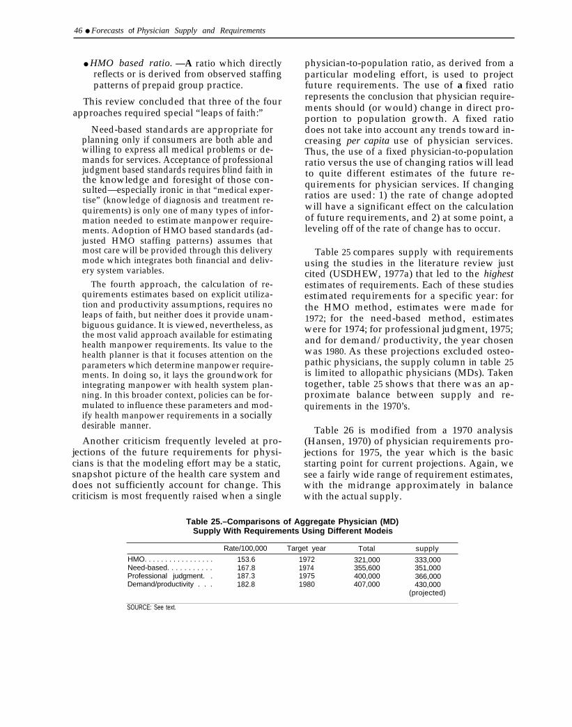
46 ● Forecasts of Physician Supply and Requirements
● HMO based ratio. —A ratio which directlyreflects or is derived from observed staffingpatterns of prepaid group practice.
This review concluded that three of the fourapproaches required special “leaps of faith:”
Need-based standards are appropriate forplanning only if consumers are both able andwilling to express all medical problems or de-mands for services. Acceptance of professionaljudgment based standards requires blind faith inthe knowledge and foresight of those con-sulted—especially ironic in that “medical exper-tise” (knowledge of diagnosis and treatment re-quirements) is only one of many types of infor-mation needed to estimate manpower require-ments. Adoption of HMO based standards (ad-justed HMO staffing patterns) assumes thatmost care will be provided through this deliverymode which integrates both financial and deliv-ery system variables.
The fourth approach, the calculation of re-quirements estimates based on explicit utiliza-tion and productivity assumptions, requires noleaps of faith, but neither does it provide unam-biguous guidance. It is viewed, nevertheless, asthe most valid approach available for estimatinghealth manpower requirements. Its value to thehealth planner is that it focuses attention on theparameters which determine manpower require-ments. In doing so, it lays the groundwork forintegrating manpower with health system plan-ning. In this broader context, policies can be for-mulated to influence these parameters and mod-ify health manpower requirements in a sociallydesirable manner.
Another criticism frequently leveled at pro-jections of the future requirements for physi-cians is that the modeling effort may be a static,snapshot picture of the health care system anddoes not sufficiently account for change. Thiscriticism is most frequently raised when a single
physician-to-population ratio, as derived from aparticular modeling effort, is used to projectfuture requirements. The use of a fixed ratiorepresents the conclusion that physician require-ments should (or would) change in direct pro-portion to population growth. A fixed ratiodoes not take into account any trends toward in-creasing per capita use of physician services.Thus, the use of a fixed physician-to-populationratio versus the use of changing ratios will leadto quite different estimates of the future re-quirements for physician services. If changingratios are used: 1) the rate of change adoptedwill have a significant effect on the calculationof future requirements, and 2) at some point, aleveling off of the rate of change has to occur.
Table 25 compares supply with requirementsusing the studies in the literature review justcited (USDHEW, 1977a) that led to the highestestimates of requirements. Each of these studiesestimated requirements for a specific year: forthe HMO method, estimates were made for1972; for the need-based method, estimateswere for 1974; for professional judgment, 1975;and for demand/productivity, the year chosenwas 1980. As these projections excluded osteo-pathic physicians, the supply column in table 25is limited to allopathic physicians (MDs). Takentogether, table 25 shows that there was an ap-proximate balance between supply and re-quirements in the 1970’s.
Table 26 is modified from a 1970 analysis(Hansen, 1970) of physician requirements pro-jections for 1975, the year which is the basicstarting point for current projections. Again, wesee a fairly wide range of requirement estimates,with the midrange approximately in balancewith the actual supply.
Table 25.–Comparisons of Aggregate Physician (MD)Supply With Requirements Using Different Modeis
Rate/100,000 Target year Total supply
HMO. . . . . . . . . . . . . . . . . 153.6 1972 321,000 333,000Need-based. . . . . . . . . . . 167.8 1974 355,600 351,000Professional judgment. . 187.3 1975 400,000 366,000Demand/productivity . . . 182.8 1980 407,000 430,000
(projected)
SOURCE: See text.
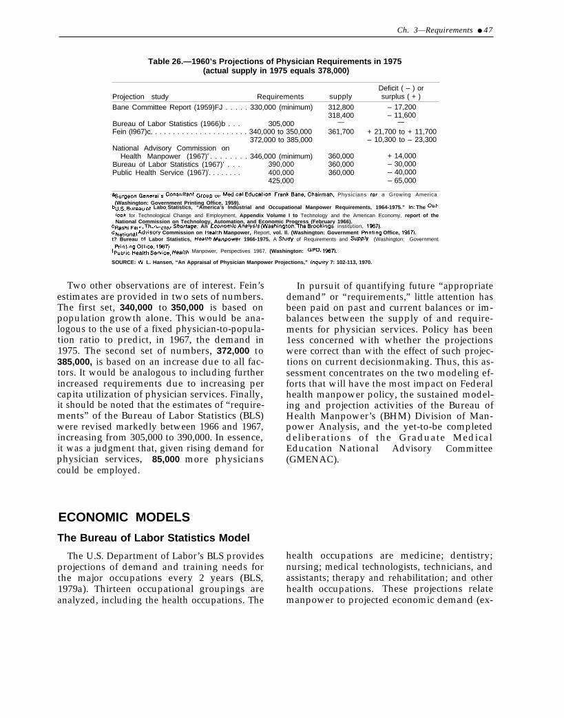
Ch. 3—Requirements ● 47
Table 26.—1960’s Projections of Physician Requirements in 1975(actual supply in 1975 equals 378,000)
Deficit ( – ) orProjection study Requirements supply surplus ( + )
Bane Committee Report (1959)FJ . . . . . 330,000 (minimum) 312,800 – 17,200318,400 – 11,600
Bureau of Labor Statistics (1966)b . . . 305,000 — —Fein (l967)c. . . . . . . . . . . . . . . . . . . . . . 340,000 to 350,000 361,700 + 21,700 to + 11,700
372,000 to 385,000 – 10,300 to – 23,300National Advisory Commission on
Health Manpower (1967)d . . . . . . . . 346,000 (minimum) 360,000 + 14,000Bureau of Labor Statistics (1967)’ . . . 390,000 360,000 – 30,000Public Health Service (1967)f. . . . . . . . 400,000 360,000 – 40,000
425,000 – 65,000
asUrQeOn General,~ cOn~Ult~nt G~~U~ on M’di~al Education, Frank Ban’, chairman, Physicians for a Growing America
(Washington: Government Printing Office, 1959).bus, Bureau of Labor Statistics, “America’s Industrial and Occupational Manpower Requirements, 1964-1975.” In: The OUf-
Iook for Technological Change and Employment, Appendix Volume I to Technology and the American Economy, report of theNational Commission on Technology, Automation, and Economic Progress (February 1966).
cRashi Fein The Doctor Shortage: An E~onom/c Ana/ysis (Washington: The Brookirlgs institution, 1967).dNatlonal A&vlso~ Commission on Health Manpower, Report, vol. Il. (Washington: Government prlntin9 Office, 1~7)t? Bureau of Labor Statistics, f-fea/th ~anpower 1966-1975, A Study of Requirements and SUPP/Y (Washington: Government
f[~~~~n~e~~~$~e’w~c~; Health Manpower, Perspectives 1967, (Washington: GpO. 1~7)
SOURCE: W, L. Hansen, “An Appraisal of Physician Manpower Projections,” Inquiry 7: 102-113, 1970.
Two other observations are of interest. Fein’sestimates are provided in two sets of numbers.The first set, 340,000 to 350,000 is based onpopulation growth alone. This would be ana-logous to the use of a fixed physician-to-popula-tion ratio to predict, in 1967, the demand in1975. The second set of numbers, 372,000 to385,000, is based on an increase due to all fac-tors. It would be analogous to including furtherincreased requirements due to increasing percapita utilization of physician services. Finally,it should be noted that the estimates of “require-ments” of the Bureau of Labor Statistics (BLS)were revised markedly between 1966 and 1967,increasing from 305,000 to 390,000. In essence,it was a judgment that, given rising demand forphysician services, 85,000 more physicianscould be employed.
ECONOMIC MODELS
The Bureau of Labor Statistics Model
In pursuit of quantifying future “appropriatedemand” or “requirements,” little attention hasbeen paid on past and current balances or im-balances between the supply of and require-ments for physician services. Policy has been1ess concerned with whether the projectionswere correct than with the effect of such projec-tions on current decisionmaking. Thus, this as-sessment concentrates on the two modeling ef-forts that will have the most impact on Federalhealth manpower policy, the sustained model-ing and projection activities of the Bureau ofHealth Manpower’s (BHM) Division of Man-power Analysis, and the yet-to-be completeddeliberations of the Graduate MedicalEducation National Advisory Committee(GMENAC).
The U.S. Department of Labor’s BLS provides health occupations are medicine; dentistry;projections of demand and training needs for nursing; medical technologists, technicians, andthe major occupations every 2 years (BLS, assistants; therapy and rehabilitation; and other1979a). Thirteen occupational groupings are health occupations. These projections relateanalyzed, including the health occupations. The manpower to projected economic demand (ex-
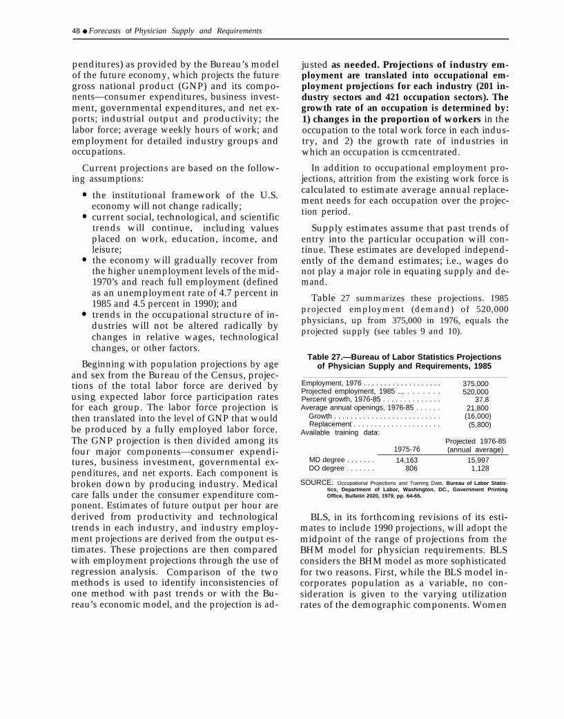
48 ● Forecasts of Physician Supply and Requirements
penditures) as provided by the Bureau’s modelof the future economy, which projects the futuregross national product (GNP) and its compo-nents—consumer expenditures, business invest-ment, governmental expenditures, and net ex-ports; industrial output and productivity; thelabor force; average weekly hours of work; andemployment for detailed industry groups andoccupations.
Current projections are based on the follow-ing assumptions:
●
●
●
●
the institutional framework of the U.S.economy will not change radically;current social, technological, and scientifictrends will continue, including valuesplaced on work, education, income, andleisure;the economy will gradually recover fromthe higher unemployment levels of the mid-1970’s and reach full employment (definedas an unemployment rate of 4.7 percent in1985 and 4.5 percent in 1990); andtrends in the occupational structure of in-dustries will not be altered radically bychanges in relative wages, technologicalchanges, or other factors.
Beginning with population projections by ageand sex from the Bureau of the Census, projec-tions of the total labor force are derived byusing expected labor force participation ratesfor each group. The labor force projection isthen translated into the level of GNP that wouldbe produced by a fully employed labor force.The GNP projection is then divided among itsfour major components—consumer expendi-tures, business investment, governmental ex-penditures, and net exports. Each component isbroken down by producing industry. Medicalcare falls under the consumer expenditure com-ponent. Estimates of future output per hour arederived from productivity and technologicaltrends in each industry, and industry employ-ment projections are derived from the output es-timates. These projections are then comparedwith employment projections through the use ofregression analysis. Comparison of the twomethods is used to identify inconsistencies ofone method with past trends or with the Bu-reau’s economic model, and the projection is ad-
justed as needed. Projections of industry em-ployment are translated into occupational em-ployment projections for each industry (201 in-dustry sectors and 421 occupation sectors). Thegrowth rate of an occupation is determined by:1) changes in the proportion of workers in theoccupation to the total work force in each indus-try, and 2) the growth rate of industries inwhich an occupation is ccmcentrated.
In addition to occupational employment pro-jections, attrition from the existing work force iscalculated to estimate average annual replace-ment needs for each occupation over the projec-tion period.
Supply estimates assume that past trends ofentry into the particular occupation will con-tinue. These estimates are developed independ-ently of the demand estimates; i.e., wages donot play a major role in equating supply and de-mand.
Table 27 summarizes these projections. 1985projected employment (demand) of 520,000physicians, up from 375,000 in 1976, equals theprojected supply (see tables 9 and 10).
Table 27.—Bureau of Labor Statistics Projectionsof Physician Supply and Requirements, 1985
Employment, 1976 . . . . . . . . . . . . . . . . . . . 375,000Projected employment, 1985 .., . . . . . . . 520,000Percent growth, 1976-85 . . . . . . . . . . . . . . 37.8Average annual openings, 1976-85 . . . . . . 21,800
Growth . . . . . . . . . . . . . . . . . . . . . . . . . . (16,000)Replacement . . . . . . . . . . . . . . . . . . . . . (5,800)
Available training data:Projected 1976-85
1975-76 (annual average)MD degree . . . . . . . 14,163 15,997DO degree . . . . . . . 806 1,128
SOURCE: Occupational Projections and Training Date, Bureau of Labor Statis-tics, Department of Labor, Washington, DC., Government PrintingOffice, Bulletin 2020, 1979, pp. 64-65.
BLS, in its forthcoming revisions of its esti-mates to include 1990 projections, will adopt themidpoint of the range of projections from theBHM model for physician requirements. BLSconsiders the BHM model as more sophisticatedfor two reasons. First, while the BLS model in-corporates population as a variable, no con-sideration is given to the varying utilizationrates of the demographic components. Women
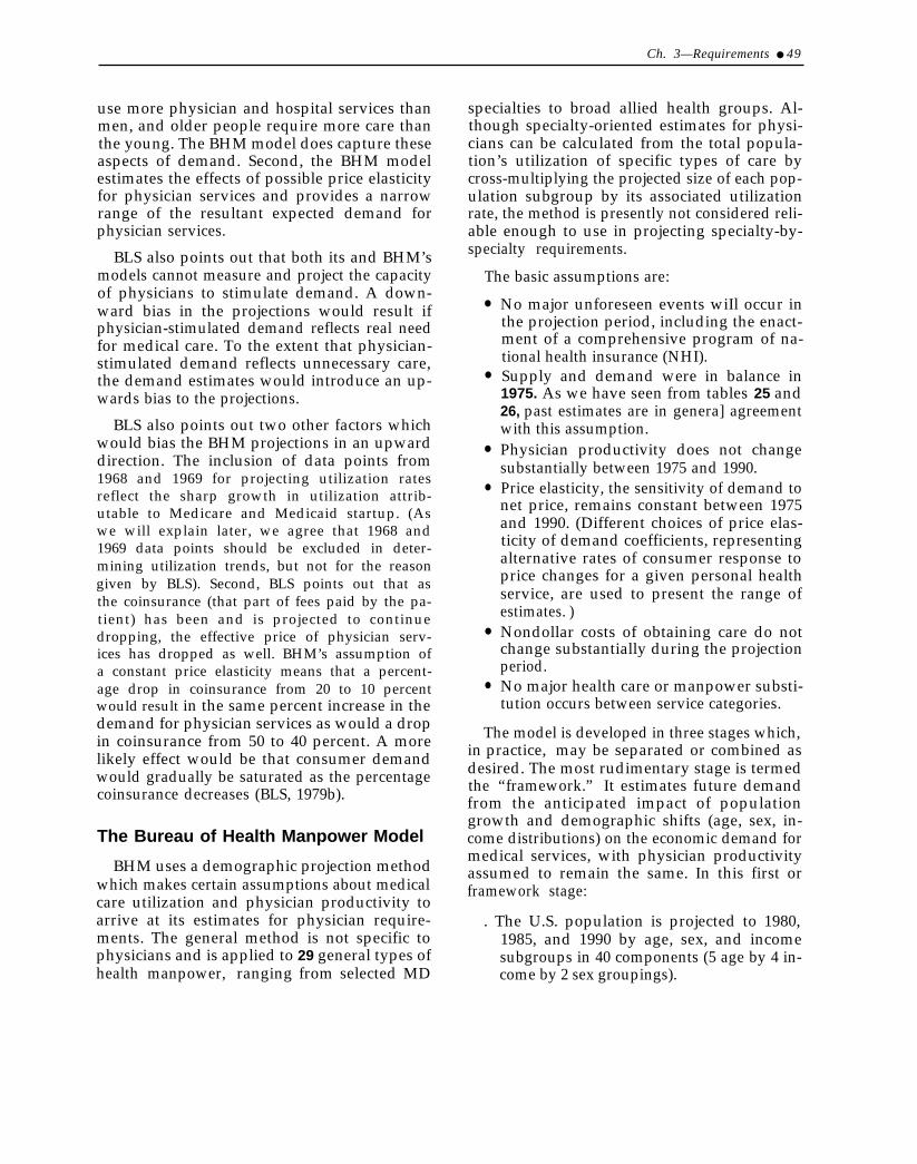
Ch. 3—Requirements ● 49
use more physician and hospital services thanmen, and older people require more care thanthe young. The BHM model does capture theseaspects of demand. Second, the BHM modelestimates the effects of possible price elasticityfor physician services and provides a narrowrange of the resultant expected demand forphysician services.
BLS also points out that both its and BHM’smodels cannot measure and project the capacityof physicians to stimulate demand. A down-ward bias in the projections would result ifphysician-stimulated demand reflects real needfor medical care. To the extent that physician-stimulated demand reflects unnecessary care,the demand estimates would introduce an up-wards bias to the projections.
BLS also points out two other factors whichwould bias the BHM projections in an upwarddirection. The inclusion of data points from1968 and 1969 for projecting utilization ratesreflect the sharp growth in utilization attrib-utable to Medicare and Medicaid startup. (Aswe will explain later, we agree that 1968 and1969 data points should be excluded in deter-mining utilization trends, but not for the reasongiven by BLS). Second, BLS points out that asthe coinsurance (that part of fees paid by the pa-tient) has been and is projected to continuedropping, the effective price of physician serv-ices has dropped as well. BHM’s assumption ofa constant price elasticity means that a percent-age drop in coinsurance from 20 to 10 percentwould result in the same percent increase in thedemand for physician services as would a dropin coinsurance from 50 to 40 percent. A morelikely effect would be that consumer demandwould gradually be saturated as the percentagecoinsurance decreases (BLS, 1979b).
The Bureau of Health Manpower Model
BHM uses a demographic projection methodwhich makes certain assumptions about medicalcare utilization and physician productivity toarrive at its estimates for physician require-ments. The general method is not specific tophysicians and is applied to 29 general types ofhealth manpower, ranging from selected MD
specialties to broad allied health groups. Al-though specialty-oriented estimates for physi-cians can be calculated from the total popula-tion’s utilization of specific types of care bycross-multiplying the projected size of each pop-ulation subgroup by its associated utilizationrate, the method is presently not considered reli-able enough to use in projecting specialty-by-specialty requirements.
The basic assumptions are:
●
●
●
●
●
●
No major unforeseen events wiIl occur inthe projection period, including the enact-ment of a comprehensive program of na-tional health insurance (NHI).Supply and demand were in balance in1975. As we have seen from tables 25 and26, past estimates are in genera] agreementwith this assumption.Physician productivity does not changesubstantially between 1975 and 1990.Price elasticity, the sensitivity of demand tonet price, remains constant between 1975and 1990. (Different choices of price elas-ticity of demand coefficients, representingalternative rates of consumer response toprice changes for a given personal healthservice, are used to present the range ofestimates. )Nondollar costs of obtaining care do notchange substantially during the projectionperiod.No major health care or manpower substi-tution occurs between service categories.
The model is developed in three stages which,in practice, may be separated or combined asdesired. The most rudimentary stage is termedthe “framework.” It estimates future demandfrom the anticipated impact of populationgrowth and demographic shifts (age, sex, in-come distributions) on the economic demand formedical services, with physician productivityassumed to remain the same. In this first orframework stage:
. The U.S. population is projected to 1980,1985, and 1990 by age, sex, and incomesubgroups in 40 components (5 age by 4 in-come by 2 sex groupings).
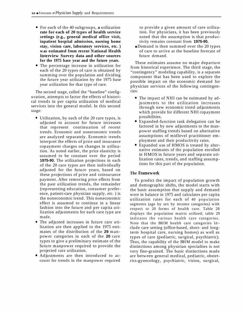
so ● Forecasts of Physician Supply and Requirements
●
●
For each of the 40 subgroups, a utilizationrate for each of 20 types of health servicesettings (e.g., general medical office visit,inpatient hospital admission, nursing homestay, vision care, laboratory services, etc. )was estimated from recent National HealthInterview Survey data and other sourcesfor the 1975 base year and the future years.The percentage increase in utilization foreach of the 20 types of care is obtained bysumming over the population and dividingthe future year utilization by the 1975 baseyear utilization for that type of care.
The second stage, called the “baseline” config-uration, attempts to factor the effects of histori-cal trends in per capita utilization of medicalservices into the general model. In this secondstage:
●
●
●
Utilization, by each of the 20 care types, isadjusted to account for future increasesthat represent continuation of recenttrends. Economic and noneconomic trendsare analyzed separately. Economic trendsinterpret the effects of price and insurancecopayment charges on changes in utiliza-tion. As noted earlier, the price elasticity isassumed to be constant over the period1975-90. The utilization projections in eachof the 20 care types are then individuallyadjusted for the future years, based onthese projections of price and coinsurancepayment. After removing price effects fromthe past utilization trends, the remainder(representing education, consumer prefer-ence, patient-care physician supply, etc. ) isthe noneconomic trend. This noneconomiceffect is assumed to continue in a linearfashion into the future and per capita uti-lization adjustments for each care type aremade.The adjusted increases in future care uti-lization are then applied to the 1975 esti-mates of the distribution of the 29 man-power categories in each of the 20 caretypes to give a preliminary estimate of thefuture manpower required to provide theprojected care utilization.Adjustments are then introduced to ac-count for trends in the manpower required
to provide a given amount of care utiliza-tion. For physicians, it has been previouslynoted that the assumption is that produc-tivity remains constant from 1975-90.
● Demand is then summed over the 20 typesof care to arrive at the baseline forecast offuture demand.
These estimates assume no major departurefrom historical experience. The third stage, the“contingency” modeling capability, is a separatecomponent that has been used to explore thepossible impact on the economic demand forphysician services of the following contingen-cies:
●
●
●
The
The impact of NHI can be estimated by ad-justments to the utilization increasesthrough new economic trend adjustmentswhich provide for different NHI copaymentpossibilities.Expanded-function task delegation can befactored in by new adjustments to the man-power staffing trends based on alternativeassumptions of midlevel practitioner em-ployment and their productivity rates.Expanded use of HMOS is treated by alter-native estimates of the population enrolledin HMOS in future years and separate uti-lization rates, trends, and staffing assump-tions for this part of the population.
Framework
To predict the impact of population growthand demographic shifts, the model starts withthe basic assumption that supply and demandwere in balance in 1975 and calculates per capitautilization rates for each of 40 populationsegments (age by sex by income categories) withrespect to 20 forms of health care. Table 28displays the population matrix utilized; table 29indicates the various health care categories.Note that the BHM health care categories in-clude care setting (office-based, short- and long-term hospital care, nursing homes) as well astypes of care (pediatric, surgical, psychiatric).Thus, the capability of the BHM model to makedistinctions among physician specialties is notvery fine-grained. The basic distinctions madeare between general medical, pediatric, obstet-rics-gynecology, psychiatric, vision, surgical,
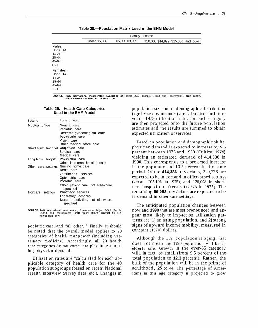
Ch. 3—Requirements . 51
Table 28.—Population Matrix Used in the BHM Model
Family income
Under $5,000 $5,000-$9,999 $10,000 -$14,999 $15,000 and over
MalesUnder 1414-2425-4445-6465+
FemalesUnder 1414-2425-4445-6465+
SOURCE. JWK International Incorporated, Evaluation of Project SOAR (Supply, Output, and Requirements), draft report,DHEW contract No. HRA 232.78-0140, 1979.
Table 29.—Health Care CategoriesUsed in the BHM Model
Setting Form of care
Medical office
Short-term hospital
Long-term hospital
Other care settings
Noncare settings
General carePediatric careObstetric-gynecological carePsychiatric careVision careOther medical office careOutpatient careSurgical careMedical carePsychiatric careOther long-term hospital careNursing home careDental careVeterinarian servicesOptometric carePodiatric careOther patient care, not elsewhere
specifiedPharmacy servicesLaboratory servicesNoncare activities, not elsewhere
specified
SOURCE JWK International Incorporated, Evaluation of Project SOAR (Supply,Output. and Requirements), draft report, DHEW contract NO HRA232;78-0140, 1979
podiatric care, and “all other. ” Finally, it shouldbe noted that the overall model applies to 29categories of health manpower (including vet-erinary medicine). Accordingly, all 20 healthcare categories do not come into play in estimat-ing physician demand.
Utilization rates are “calculated for each ap-plicable category of health care for the 40population subgroups (based on recent NationalHealth Interview Survey data, etc.). Changes in
population size and in demographic distribution(age by sex by incomes) are calculated for futureyears. 1975 utilization rates for each categoryare then projected onto the future populationestimates and the results are summed to obtainexpected utilization of services.
Based on population and demographic shifts,physician demand is expected to increase by 9.5percent between 1975 and 1990 (Cultice, 1979)yielding an estimated demand of 414,336 in1990. This corresponds to a projected increasein the population of 10.5 percent in the sameperiod. Of the 414,336 physicians, 229,276 areexpected to be in demand in office-based settings(versus 205,196 in 1975), and 126,008 in short-term hospital care (versus 117,573 in 1975). Theremaining 59,052 physicians are expected to bein demand in other care settings.
The anticipated population changes betweennow and 1990 that are most pronounced and ap-pear most likely to impact on utilization pat-terns are: 1) an aging population, and 2) strongsigns of upward income mobility, measured inconstant (1970) dollars.
Although the U.S. population is aging, thatdoes not mean the 1990 population will be anelderly one. Growth in the over-65 categorywill, in fact, be small (from 9.5 percent of thetotal population to 12.3 percent). Rather, thebulk of the population will be in the prime ofadulthood, 25 to 44. The percentage of Amer-icans in this age category is projected to grow
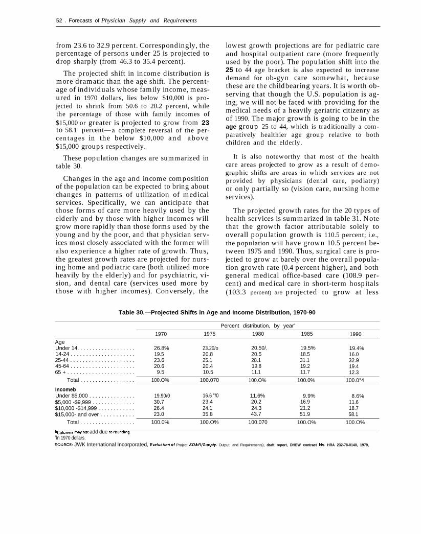
52 . Forecasts of Physician Supply and Requirements
from 23.6 to 32.9 percent. Correspondingly, thepercentage of persons under 25 is projected todrop sharply (from 46.3 to 35.4 percent).
The projected shift in income distribution ismore dramatic than the age shift. The percent-age of individuals whose family income, meas-ured in 1970 dollars, lies below $10,000 is pro-jected to shrink from 50.6 to 20.2 percent, whilethe percentage of those with family incomes of$15,000 or greater is projected to grow from 23to 58.1 percent— a complete reversal of the per-centages in the below $10,000 and above$15,000 groups respectively.
These population changes are summarized intable 30.
Changes in the age and income compositionof the population can be expected to bring aboutchanges in patterns of utilization of medicalservices. Specifically, we can anticipate thatthose forms of care more heavily used by theelderly and by those with higher incomes willgrow more rapidly than those forms used by theyoung and by the poor, and that physician serv-ices most closely associated with the former willalso experience a higher rate of growth. Thus,the greatest growth rates are projected for nurs-ing home and podiatric care (both utilized moreheavily by the elderly) and for psychiatric, vi-sion, and dental care (services used more bythose with higher incomes). Conversely, the
lowest growth projections are for pediatric careand hospital outpatient care (more frequentlyused by the poor). The population shift into the25 to 44 age bracket is also expected to increasedemand for ob-gyn care somewhat, becausethese are the childbearing years. It is worth ob-serving that though the U.S. population is ag-ing, we will not be faced with providing for themedical needs of a heavily geriatric citizenry asof 1990. The major growth is going to be in theage group 25 to 44, which is traditionally a com-paratively healthier age group relative to bothchildren and the elderly.
It is also noteworthy that most of the healthcare areas projected to grow as a result of demo-graphic shifts are areas in which services are notprovided by physicians (dental care, podiatry)or only partially so (vision care, nursing homeservices).
The projected growth rates for the 20 types ofhealth services is summarized in table 31. Notethat the growth factor attributable solely tooverall population growth is 110.5 percent; i.e.,the population will have grown 10.5 percent be-tween 1975 and 1990. Thus, surgical care is pro-jected to grow at barely over the overall popula-tion growth rate (0.4 percent higher), and bothgeneral medical office-based care (108.9 per-cent) and medical care in short-term hospitals(103.3 percent) are projected to grow at less
Table 30.—Projected Shifts in Age and Income Distribution, 1970-90
Percent distribution, by yeara
1970 1975 1980 1985 1990
AgeUnder 14. . . . . . . . . . . . . . . . . . . 26.8% 23.20/o 20.50/. 19.5% 19.4%14-24 . . . . . . . . . . . . . . . . . . . . . 19.5 20.8 20.5 18.5 16.025-44 . . . . . . . . . . . . . . . . . . . . . 23.6 25.1 28.1 31.1 32.945-64 . . . . . . . . . . . . . . . . . . . . . 20.6 20.4 19.8 19.2 19.465 + . . . . . . . . . . . . . . . . . . . . . . 9.5 10.5 11.1 11.7 12.3
Total . . . . . . . . . . . . . . . . . . 100.O% 100.070 100.O% 100.0% 100.0°4
IncomebUnder $5,000 . . . . . . . . . . . . . . . 19.90/0 16.6 ”/0 11.6% 9.9% 8.6%$5,000 -$9,999 . . . . . . . . . . . . . . 30.7 23.4 20.2 16.9 11.6$10,000 -$14,999 . . . . . . . . . . . . 26.4 24.1 24.3$15,000- and over . . . . . . . . . . .
21.2 18.723.0 35.8 43.7 51.9 58.1
Total . . . . . . . . . . . . . . . . . . 100.0% 100.O% 100.070 100.O% 100.O%
acOlumnS may not add due to rounding.bln 1970 dollars.SOURCE: JWK International Incorporated, Ev81u~f/orr of Project SOAR(Supp/y, Output, and Requirements), draft report, DHEW contract No. HRA 232-78-0140, 1979,
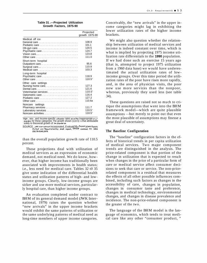
C h . 3 - R e q u i r e r n e t I t S ● 5 3
Table 31 .—Projected UtilizationGrowth Factors, 1975-90
Projectedgrowth 1975-90
Medical off iceGeneral care . . . . . . . . . . . . . . . . . . . . . . . . . . 108.9Pediatric care . . . . . . . . . . . . . . . . . . . . . . . . . 101.1Ob-gyn care. . . . . . . . . . . . . . . . . . . . . . . . . . . 120.5Psychiatric care . . . . . . . . . . . . . . . . . . . . . . . 124.7Vision care..... . . . . . . . . . . . . . . . . . . . . . . . 123.8Other care . . . . . . . . . . . . . . . . . . . . . . . . . . . . 111.0
Short-term hospitalOutpatient care. . . . . . . . . . . . . . . . . . . . . . . . 95.6Surgical care.... . . . . . . . . . . . . . . . . . . . . . . 110.9Medical care . . . . . . . . . . . . . . . . . . . . . . . . . . 103.3Long-term hospitalPsychiatric care . . . . . . . . . . . . . . . . . . . . . . . 118.9Other care . . . . . . . . . . . . . . . . . . . . . . . . . . . . 110.5 a
Other care settingsNursing home care. . . . . . . . . . . . . . . . . . . . . 127.3Dental care. . . . . . . . . . . . . . . . . . . . . . . . . . . . 121.6Veterinarian services . . . . . . . . . . . . . . . . . . . 110.5a
Optometric care . . . . . . . . . . . . . . . . . . . . . . . 116.4Podiatric care . . . . . . . . . . . . . . . . . . . . . . . . . 127.2Other care . . . . . . . . . . . . . . . . . . . . . . . . . . . . 110.6a
Noncare settingsPharmacy services . . . . . . . . . . . . . . . . . . . . . 111.7Laboratory services . . . . . . . . . . . . . . . . . . . . 110.5 a
Noncare activities. . . . . . . . . . . . . . . . . . . . . . 110.5 a
aAge-, sex-, and Income-specific utll!zatlon rates areei(her inappropriate orun-avallable for these categories The growth shown (110.5) IS that attributablesolely to theoverall growth of thepopulat!on.
SOURCE. JWKlnternatlonal incorporated,.EvaluatiOfl of Pro/ect SOAR(Supp/y,OIJtpuL and Requ/rernenfs), draft report, DHEW contract No. HRA232.78-0140,1979.
than the overall population growth rate of 110.5percent.
These projections deal with utilization ofmedical services as an expression of economicdemand, not medical need. We do know, how-ever, that higher income has traditionally beenassociated with improvements in health status;i.e., less need for medical care. Tables 32 t0 35give some indication of the differential healthstatus and utilization patterns of high- and low-income groups. Clearly, low-income groups aresicker and use more medical services, particular-ly hospital care, than higher income groups.
An evaluation completed under contract toBHM of its general demand model (JWK Inter-national, 1979) raises the question whether“new arrivals” in the upper income bracketswould exhibit the same patterns of utilization orthe same underlying patterns of medical need aslong-time members of upper income categories.
Conceivably, the “new arrivals” in the upper in-come categories might lag in exhibiting thelower utilization rates of the higher incomebrackets.
We might also question whether the relation-ship between utilization of medical services andincome is indeed constant over time, which iswhat is implied by projecting 1975 income uti-lization rate differentials to the 1990 population.If we had done such an exercise 15 years ago(that is, attempted to project 1975 utilizationfrom a 1960 data base) we would have underes-timated the actual utilization rates of low-income groups. Over this time period the utili-zation rates of the poor have risen more rapidly,and, in the area of physician visits, the poornow use more services than the nonpoor,whereas, previously they used less (see table34).
These questions are raised not so much to cri-tique the assumptions that went into the BHMframework model—which are quite plausibleassumptions —but merely to point out that eventhe most plausible of assumptions may finesse agreat deal of uncertainty.
The Baseline Configuration
The “baseline” configuration factors in the ef-fects of historical trends in per capita utilizationof medical services. Two major componenttrends are distinguished in the analysis. Theprice-related component is that portion of thechange in utilization that is expected to resultwhen changes in the price of a particular form ofcare or medical service affect consumer deci-sions to seek that care or service. The non-price-related component is a residual that measuresthe effects of all other possible influences com-bined, including such factors as changes in theaccessibility of care, changes in population,changes in consumer taste and preference,changes in medical technology, environmentalchanges, and changes in disease prevalence andincidence. The non-price-related component isthe greater of the two.
The language of the BHM model is the lan-guage of economics, which tends to treat medi-cal care like any other “consumer product, ”
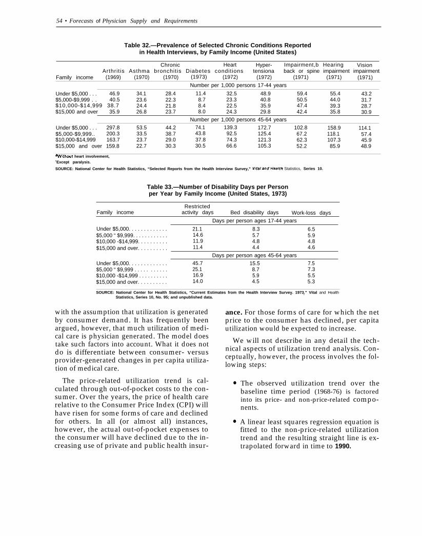
54 • Forecasts of Physician Supply and Requirements
Table 32.—Prevalence of Selected Chronic Conditions Reportedin Health Interviews, by Family Income (United States)
Chronic Heart Hyper- Impairment,b Hearing VisionArthrit is Asthma bronchit is Diabetes condit ions tensiona back or spine impairment impairment
Family income (1969) (1970) (1970) (1973) (1972) (1972) (1971) (1971) (1971)
Number per 1,000 persons 17-44 years
Under $5,000 . . . 46.9 34.1 28.4 11.4 32.5 48.9 59.4 55.4 43.2$5,000-$9,999 . . 40.5 23.6 22.3 8.7 23.3 40.8 50.5 44.0 31.7$10,000-$14,999 38.7 24.4 21.8 8.4 22.5 35.9 47.4 39.3 28.7$15,000 and over 35.9 26.8 23.7 8.0 24.3 29.8 42.4 35.8 30.9
Number per 1,000 persons 45-64 years
Under $5,000 . . . 297.8 53.5 44.2 74.1 139.3 172.7 102.8$5,000-$9,999..
158.9 114.1200.3 33.5 38.7 43.8 92.5 125.4 67.2 118.1 57.4
$10,000-$14,999 163.7 23.7 29.0 37.8 74.3 121.3$15,000 and over 159.8
62.3 107.3 45.922.7 30.3 30.5 66.6 105.3 52.2 85.9 48.9
awithout heart involvement,bExcept paralysis.
SOURCE: National Center for Health Statistics, “Selected Reports from the Health Interview Survey,” Vita/ and Hea/th Statistics, Series 10.
Table 33.—Number of Disability Days per Personper Year by Family Income (United States, 1973)
RestrictedFamily income activity days Bed disability days Work-loss days
Days per person ages 17-44 years
Under $5,000. . . . . . . . . . . . . 21.1 8.3 6.5$5,000 “ $9,999. . . . . . . . . . . . 14.6 5.7 5.9$10,000 -$14,999. . . . . . . . . .$15,000 and over. . . . . . . . . .
11.9 4.8 4.811.4 4.4 4.6
Days per person ages 45-64 years
Under $5,000. . . . . . . . . . . . . 45.7 15.5 7.5$5,000 “ $9,999 . . . . . . . . . . . 25.1 8.7 7.3$10,000 -$14,999 . . . . . . . . . .$15,000 and over. . . . . . . . . .
16.9 5.9 5.514.0 4.5 5.3
SOURCE: National Center for Health Statistics, “Current Estimates from the Health Interview Survey. 1973.” Vital and HealthStatistics, Series 10, No. 95; and unpublished data.
. .
with the assumption that utilization is generatedby consumer demand. It has frequently beenargued, however, that much utilization of medi-cal care is physician generated. The model doestake such factors into account. What it does notdo is differentiate between consumer- versusprovider-generated changes in per capita utiliza-tion of medical care.
The price-related utilization trend is cal-culated through out-of-pocket costs to the con-sumer. Over the years, the price of health carerelative to the Consumer Price Index (CPI) willhave risen for some forms of care and declinedfor others. In all (or almost all) instances,however, the actual out-of-pocket expenses tothe consumer will have declined due to the in-creasing use of private and public health insur-
ance. For those forms of care for which the netprice to the consumer has declined, per capitautilization would be expected to increase.
We will not describe in any detail the tech-nical aspects of utilization trend analysis. Con-ceptually, however, the process involves the fol-lowing steps:
●
●
The observed utilization trend over thebaseline time period (1968-76) is factoredinto its price- and non-price-related compo-nents.
A linear least squares regression equation isfitted to the non-price-related utilizationtrend and the resulting straight line is ex-trapolated forward in time to 1990.
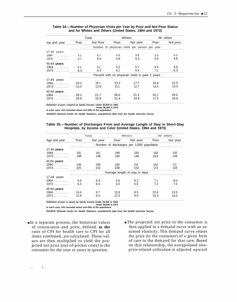
Ch. 3—Requireme?zts ● 55
Table 34.—Number of Physician Visits per Year by Poor and Not Poor Statusand for Whites and Others (United States, 1964 and 1973)
Total Whites All others
Aae and year Poor Not Poor Poor Not poor Poor Not poorNumber of physician visits per person per year
17-44 years1964 . . . . . . . . . 4.1 4.7 4.5 4.8 3.3 4.21973 . . . . . . . . . 5.7 5.0 5.8 5.0 5.6 4.8
45-64 years1964 . . . . . . . . . 5.1 5.1 5.2 5.1 4.9 4.61973 . . . . . . . . . 6.3 5.4 6.1 5.4 7.1 5.3
Percent with no physican visits in past 2 years
17.44 years1964 . . . . . . . . . 24.2 18.1 23.2 17.7 26.6 22.91973 . . . . . . . . . 13.4 12.8 13.1 12.7 14.5 13.5
45-64 years1964 . . . . . . . . . 29.2 21.7 28.0 21.3 33.1 29.01973 . . . . . . . . . 20.6 16.9 21.4 16.9 17.0 16.9
Definition of poor IS based on family Income. Under $3,000 in 1964.Under $6,000 in 1973
In each case, this included about one.fifth of the population.
SOURCE National Center for Health Statistics, unpublished data from the Health Interview Survey
Table 35.—Number of Discharges From and Average Length of Stay in Short-StayHospitals, by Income and Color (United States, 1964 and 1973)
Total Whi tes All others
Age and year Poor Not poor Poor Not poor Poor Not poor
Number of discharges per 1,000 population
17.44 years1964 . . . . . . . . . 181 161 188 164 163 1321973 . . . . . . . . . 198 148 190 148 223 149
45.64 years1964 . . . . . . . . . 146 148 159 151 102 1111973 . . . . . . . . . 225 152 238 153 174 133
Average length of stay in days
17-44 years1964 . . . . . . . . . 6.9 6.3 6.8 6.2 7.1 8.01973 . . . . . . . . . 6.4 6.0 6.0 5.9 7.2 7.0
45-64 years1964 . . . . . . . . . 14.4 9.7 12.8 9.5 22.6 13.51973 . . . . . . . . . 12.8 9.3 12.3 9.0 15.3 13.0
Definition of poor is based on family Income Under $3,000 in 1964Under $6,000 in 1973
In each case, this Included about one-fifth of the population
SOURCE National Center for Health Statistics, unpublished data from the Health Interview Survey
● In a separate process, the historical values ● The projected net price to the consumer isof coinsurance and price, defined as the then applied to a demand curve with an as-ratio of CPI for health care to CPI for all sumed elasticity. This demand curve relatesitems combined, are calculated. These val- the price (to the consumer) of a given formues are then multiplied to yield the pro- of care to the demand for that care. Basedjected net price (out-of-pocket costs) to the on that relationship, the extrapolated non-consumer for the year or years in question. price-related utilization is adjusted upward
– r 1 -
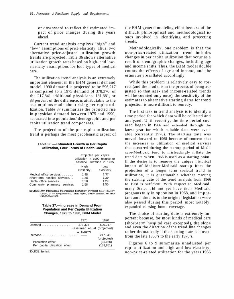
56 . Forecasts of Physician Supply and Requirements
or downward to reflect the estimated im-pact of price changes during the yearsahead.
Current trend analysis employs “high” and“low” assumptions of price elasticity. Thus, twoalternative price-adjusted utilization growthtrends are projected. Table 36 shows alternativeutilization growth rates based on high- and low-elasticity assumptions for four types of medicalcare.
The utilization trend analysis is an extremelyimportant element in the BHM general demandmodel. 1990 demand is projected to be 596,217as compared to a 1975 demand of 378,376. ofthe 217,841 additional physicians, 181,881, or83 percent of the difference, is attributable to theassumptions made about rising per capita uti-lization. Table 37 summarizes the projected risein physician demand between 1975 and 1990,separated into population/demographic and percapita utilization trend components.
The projection of the per capita utilizationtrend is perhaps the most problematic aspect of
Table 36.—Estimated Growth in Per CapitaUtilization, Four Forms of Health Care
Projected per capitautilization in 1990 relative tobaseline utilization in 1975
High Lowelasticity elasticity
Medical office services . . . . . . 1.45 1.37Short-term hospital services. . 1.38 1.29Dental office services . . . . . . . 1.28 1.29Community pharmacy services 1.58 1.50
SOURCE: JWK International Incorporated, Eva/uatiorr of Project SOAR (SIJpp/y,Output, arr~ Efequiremerrfs), draft report, DHEW contract No. HRA232-78-0140,1979.
Table 37.—increase in Demand FromPopulation and Per Capita UtilizationChanges, 1975 to 1990, BHM Model
1975 1990
Demand . . . . . . . . . . . . . . . . . . 378,376 596,217(assumed equal (projected)
to supply)Increase. . . . . . . . . . . . . . . . . . —— 217,841
(projected)Population effect . . . . . . . . (35,960)Per capita utilization effect (181,881)
SOURCE: See text.
the BHM general modeling effort because of thedifficult philosophical and methodological is-sues involved in identifying and projectingtrends.
Methodologically, one problem is that thenon-price-related utilization trend includeschanges in per capita utilization that occur as aresult of demographic changes, including ageand income shifts. Thus, the BHM model doublecounts the effects of age and income, and theestimates are inflated accordingly.
While this problem is relatively easy to cor-rect (and the model is in the process of being ad-justed so that age- and income-related trendswill be counted only once), the sensitivity of theestimates to alternative starting dates for trendprojection is more difficult to remedy.
The first task in trend analysis is to identify atime period for which data will be collected andanalyzed. Until recently, the time period cov-ered began in 1966 and extended through thelatest year for which suitable data were avail-able (currently 1976). The starting date wasmoved forward to 1968 because of concern thatthe increases in utilization of medical servicesthat occurred during the startup period of Medi-care-Medicaid tend to misleadingly inflate thetrend data when 1966 is used as a starting point.If the desire is to remove the unique historicalimpact of Medicare-Medicaid startup from theprojection of a longer term societal trend inutilization, it is questionable whether movingthe starting date of the trend analysis from 1966to 1968 is sufficient. With respect to Medicaid,many States did not yet have their Medicaidprograms fully in operation in 1968, and impor-tant amendments to the original legislation werealso passed during this period, most notably,expanded nursing home coverage.
The choice of starting date is extremely im-portant because, for most kinds of medical care(short-term hospital care excepted), the slopeand even the direction of the trend line changesrather dramatically if the starting date is movedfrom the late 1960’s to the early 1970’s.
Figures 6 to 9 summarize unadjusted percapita utilization and high and low elasticity,non-price-related utilization for the years 1966
Ch. 3—Requirements • 57
Figure 6.— Per Capita Utilization of Physician Office Services, 1966-76
Per capita utilization(visits per year)
5.00
4.75
4.50
4,25
4.00
3.75
3.50
3.25
3.00
.
.
.
.
.
.
//
● ❞ ● ✍ ✎
J * ● -% ● - ●
— - - - # - / Legend “ - “ M
*
-“ \ / Historic utilization
/‘\ ●
— ( u n a d j u s t e d )Non=prJce-relaWd utilization
“ ~ , ~ “ ‘ ~- ( I o w - e l a s t i c i t y )
— * — Non-price-related utilization(Mgh-eia$ticity)
I 1 1 I I I I I 1 I1966 1967 1968 1969 1970 1971 1972 1973 1974 1975 1976
Year
SOURCE JWK International. Inc , Evaluation 0f Project SOAR (Supply, Output, and Requirements), draft report, DHEW contract NoHRA 232.780140, 1979
to 1976. Only one set of data points (utilizationof short-term hospital services) displays a con-sistent, natural linear trend. In the case of theother services (physician office visits, dentalcare, community pharmacy), the utilizationdata being extrapolated do not consistently dis-play a pattern for which linear extrapolationcan be justified.
The mathematics of trend projection (linearregression analysis) involves fitting a straightline to the data points. Clearly, such a concep-tual simplification of reality is less distorting ofthe world’s true complexity when the datapoints themselves tend naturally to conform toa straight line pattern when graphically por-trayed. Philosophically, the issue is one of con-sistency. Trend projection in general and themethodology of linear regression in particularassume that reality—in this instance per capitautilization of medical care—exhibits a reason-
ably consistent pattern; whether it be one of in-creasing, decreasing, or remaining steady.
Figures 10 to 13 take the high-elasticity datapoints of figures 6 to 9 and fit straight lines tothe data points for the years 1966-76, 1968-76,and 1971-76. Except for short-term hospitalservices, distinctly different trends can be pro-jected, depending on the starting date. For phy-sician office services, a start date of either 1966or 1968 is seen to yield a distinctly upwardtrend, whereas a start date of 1971 shows adownward slope. In the case of dental officevisits, starting the trend analysis in 1968 pro-duces a flat projection; starting in 1971 producesa decline. For community pharmacy services,the trend lines started in 1966 and 1968 show asharp upward rise even though per capita uti-lization has been declining since 1973.
The magnitude of the disparities in per capitautilization growth produced by different startdates is quantified in table 38.
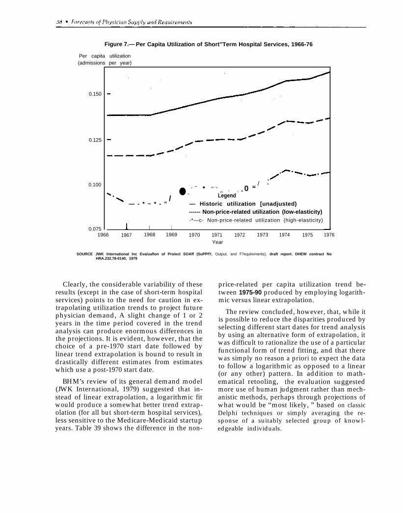
Figure 7.— Per Capita Utilization of Short”Term Hospital Services, 1966-76
Per capita utilization(admissions per year)
0.150
0.125
0.100
0.075
/ -. - ● ✍ ✎
● ✏✍ ‘ - * 0 “
/ Legend— - * ~ * - ” — Historic utilization [unadjusted)
------ Non-price-related utilization (Iow-elasticity)-*—c- Non-price-related utilization (high-elasticity)
I 11966 1967 1968 1969 1970 1971 1972 1973 1974 1975 1976
Year
SOURCE JWK International Inc Eva/uaflon of Pro/ect SOAff (SuPPfY, Output, and F?equlrements), draft report. DHEW contract NoHRA.232.78-0140, 1979
Clearly, the considerable variability of theseresults (except in the case of short-term hospitalservices) points to the need for caution in ex-trapolating utilization trends to project futurephysician demand, A slight change of 1 or 2years in the time period covered in the trendanalysis can produce enormous differences inthe projections. It is evident, however, that thechoice of a pre-1970 start date followed bylinear trend extrapolation is bound to result indrastically different estimates from estimateswhich use a post-1970 start date.
BHM’s review of its general demand model(JWK International, 1979) suggested that in-stead of linear extrapolation, a logarithmic fitwould produce a somewhat better trend extrap-olation (for all but short-term hospital services),less sensitive to the Medicare-Medicaid startupyears. Table 39 shows the difference in the non-
price-related per capita utilization trend be-tween 1975-90 produced by employing logarith-mic versus linear extrapolation.
The review concluded, however, that, while itis possible to reduce the disparities produced byselecting different start dates for trend analysisby using an alternative form of extrapolation, itwas difficult to rationalize the use of a particularfunctional form of trend fitting, and that therewas simply no reason a priori to expect the datato follow a logarithmic as opposed to a linear(or any other) pattern. In addition to math-ematical retooling, the evaluation suggestedmore use of human judgment rather than mech-anistic methods, perhaps through projections ofwhat would be “most likely, ” based on classicDelphi techniques or simply averaging the re-sponse of a suitably selected group of knowl-edgeable individuals.
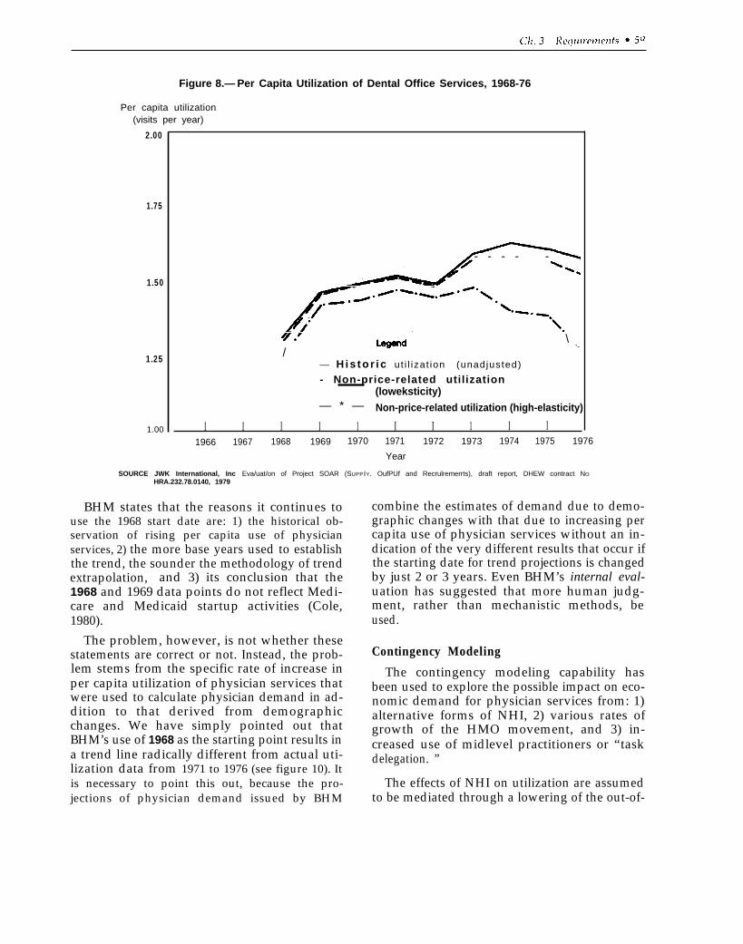
Figure 8.— Per Capita Utilization of Dental Office Services, 1968-76
Per capita utilization(visits per year)
2.00
1.75
1.50
1.25
1.00
- - - - -
/\
“~
— His tor ic ut i l izat ion (unadjusted)
- Non-price-related utilization(loweksticity)
— * — Non-price-related utilization (high-elasticity)
I I I I 1 I I 1 I I1966 1967 1968 1969 1970 1971 1972 1973 1974 1975 1976
Year
SOURCE JWK International, Inc Eva/uat/on of Project SOAR (SUPP IY. OufPUf and Recrulremerrts), draft report, DHEW contract NO
HRA.232.78.0140, 1979
BHM states that the reasons it continues touse the 1968 start date are: 1) the historical ob-servation of rising per capita use of physicianservices, 2) the more base years used to establishthe trend, the sounder the methodology of trendextrapolation, and 3) its conclusion that the1968 and 1969 data points do not reflect Medi-care and Medicaid startup activities (Cole,1980).
The problem, however, is not whether thesestatements are correct or not. Instead, the prob-lem stems from the specific rate of increase inper capita utilization of physician services thatwere used to calculate physician demand in ad-dition to that derived from demographicchanges. We have simply pointed out thatBHM’s use of 1968 as the starting point results ina trend line radically different from actual uti-lization data from 1971 to 1976 (see figure 10). Itis necessary to point this out, because the pro-jections of physician demand issued by BHM
combine the estimates of demand due to demo-graphic changes with that due to increasing percapita use of physician services without an in-dication of the very different results that occur ifthe starting date for trend projections is changedby just 2 or 3 years. Even BHM’s internal eval-uation has suggested that more human judg-ment, rather than mechanistic methods, beused.
Contingency Modeling
The contingency modeling capability hasbeen used to explore the possible impact on eco-nomic demand for physician services from: 1)alternative forms of NHI, 2) various rates ofgrowth of the HMO movement, and 3) in-creased use of midlevel practitioners or “taskdelegation. ”
The effects of NHI on utilization are assumedto be mediated through a lowering of the out-of-
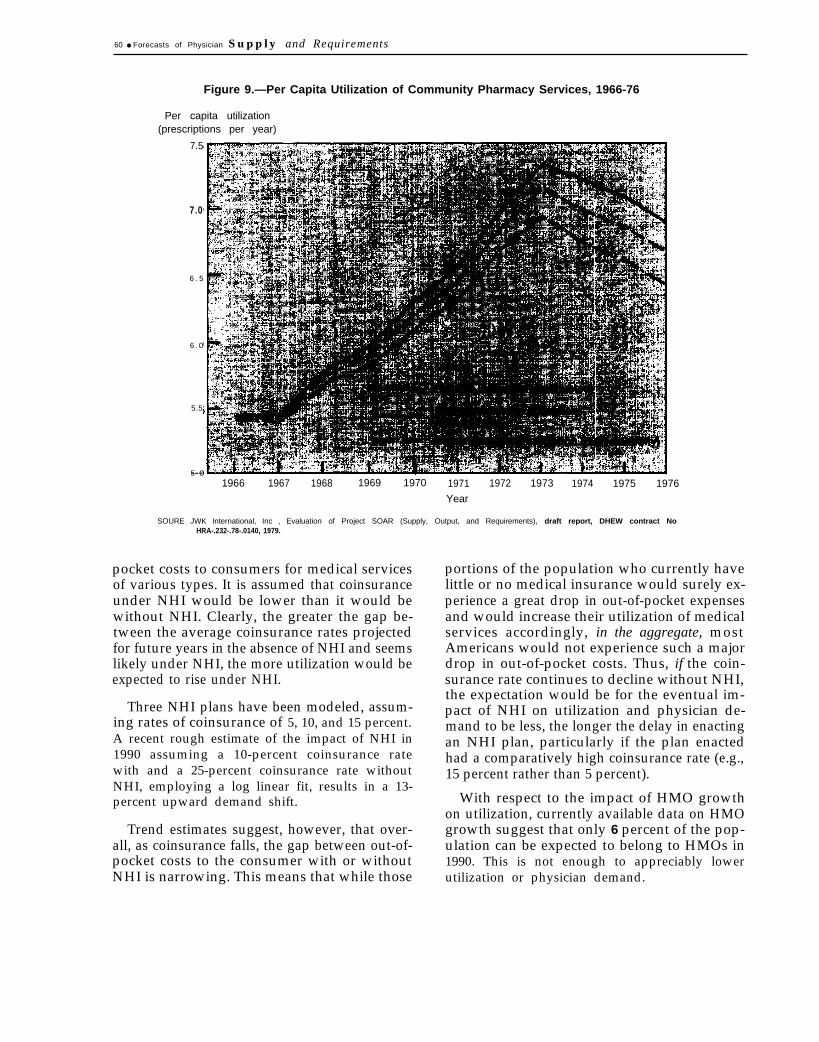
.
60 ● Forecasts of Physician Supply and Requirements
Figure 9.—Per Capita Utilization of Community Pharmacy Services, 1966-76
Per capita utilization(prescriptions per year)
7.5
7.0
6 . 5
6 . 0
5.5
5 0---1966 1967 1968 1969 1970 1971 1972 1973 1974 1975 1976
Year
SOURE JWK International, Inc , Evaluation of Project SOAR (Supply, Output, and Requirements), draft report, DHEW contract NoHRA-.232-.78-.0140, 1979.
pocket costs to consumers for medical servicesof various types. It is assumed that coinsuranceunder NHI would be lower than it would bewithout NHI. Clearly, the greater the gap be-tween the average coinsurance rates projectedfor future years in the absence of NHI and seemslikely under NHI, the more utilization would beexpected to rise under NHI.
Three NHI plans have been modeled, assum-ing rates of coinsurance of 5, 10, and 15 percent.A recent rough estimate of the impact of NHI in1990 assuming a 10-percent coinsurance ratewith and a 25-percent coinsurance rate withoutNHI, employing a log linear fit, results in a 13-percent upward demand shift.
Trend estimates suggest, however, that over-all, as coinsurance falls, the gap between out-of-pocket costs to the consumer with or withoutNHI is narrowing. This means that while those
portions of the population who currently havelittle or no medical insurance would surely ex-perience a great drop in out-of-pocket expensesand would increase their utilization of medicalservices accordingly, in the aggregate, mostAmericans would not experience such a majordrop in out-of-pocket costs. Thus, if the coin-surance rate continues to decline without NHI,the expectation would be for the eventual im-pact of NHI on utilization and physician de-mand to be less, the longer the delay in enactingan NHI plan, particularly if the plan enactedhad a comparatively high coinsurance rate (e.g.,15 percent rather than 5 percent).
With respect to the impact of HMO growthon utilization, currently available data on HMOgrowth suggest that only 6 percent of the pop-ulation can be expected to belong to HMOs in1990. This is not enough to appreciably lowerutilization or physician demand.
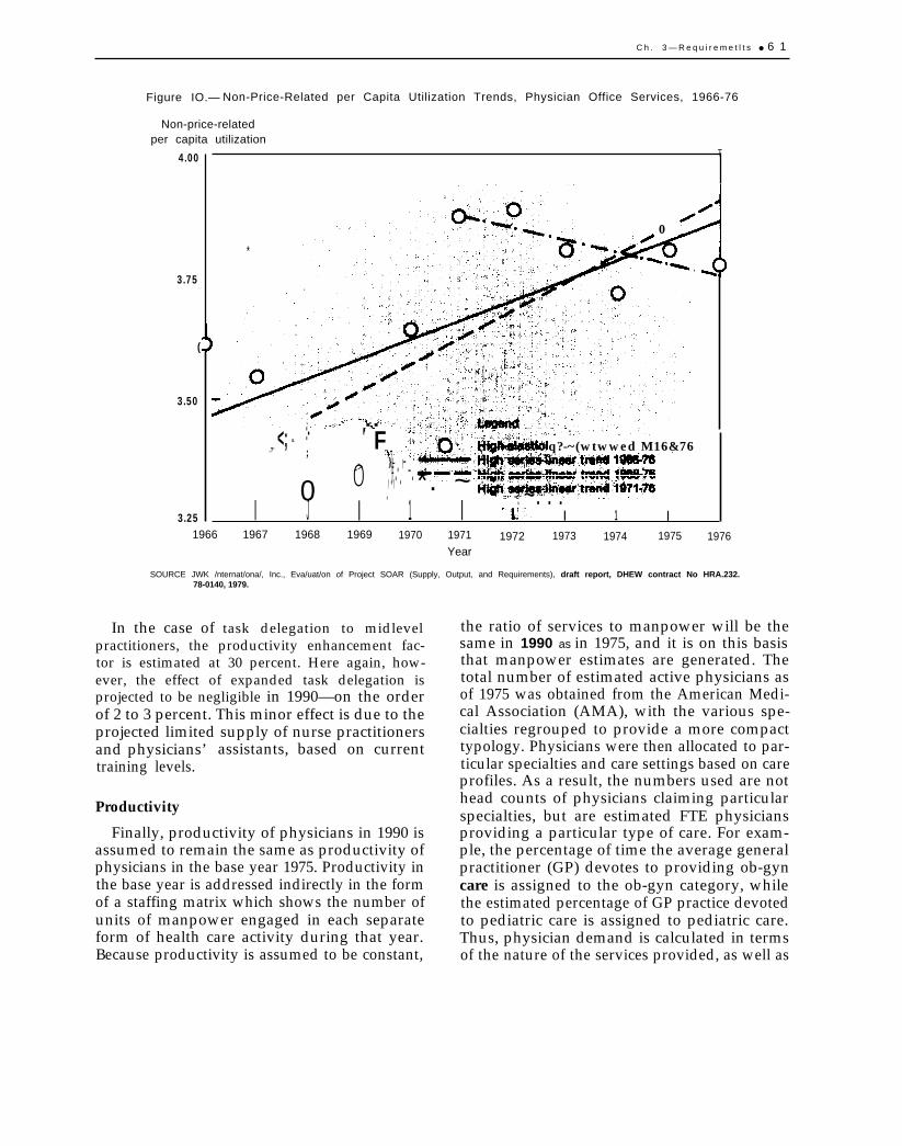
C h . 3 — R e q u i r e m e t l t s ● 6 1
Figure IO.— Non-Price-Related per Capita Utilization Trends, Physician Office Services, 1966-76
Non-price-relatedper capita utilization
4.00
3.75
(
3.50
3.25
T
*
0
.
F.- -.:-<; “
.?’ q?-~(wtwwed M16&76;}-.>0 7 . -#. ‘ -.,., .0 *. ~. :! ~. . :I J I 1 I I 1 I
1966 1967 1968 1969 1970 1971 1972 1973 1974 1975 1976Year
SOURCE JWK /nternat/ona/, Inc., Eva/uat/on of Project SOAR (Supply, Output, and Requirements), draft report, DHEW contract No HRA.232.78-0140, 1979.
In the case of task delegation to midlevelpractitioners, the productivity enhancement fac-tor is estimated at 30 percent. Here again, how-ever, the effect of expanded task delegation isprojected to be negligible in 1990—on the orderof 2 to 3 percent. This minor effect is due to theprojected limited supply of nurse practitionersand physicians’ assistants, based on currenttraining levels.
Productivity
Finally, productivity of physicians in 1990 isassumed to remain the same as productivity ofphysicians in the base year 1975. Productivity inthe base year is addressed indirectly in the formof a staffing matrix which shows the number ofunits of manpower engaged in each separateform of health care activity during that year.Because productivity is assumed to be constant,
the ratio of services to manpower will be thesame in 1990 as in 1975, and it is on this basisthat manpower estimates are generated. Thetotal number of estimated active physicians asof 1975 was obtained from the American Medi-cal Association (AMA), with the various spe-cialties regrouped to provide a more compacttypology. Physicians were then allocated to par-ticular specialties and care settings based on careprofiles. As a result, the numbers used are nothead counts of physicians claiming particularspecialties, but are estimated FTE physiciansproviding a particular type of care. For exam-ple, the percentage of time the average generalpractitioner (GP) devotes to providing ob-gyncare is assigned to the ob-gyn category, whilethe estimated percentage of GP practice devotedto pediatric care is assigned to pediatric care.Thus, physician demand is calculated in termsof the nature of the services provided, as well as
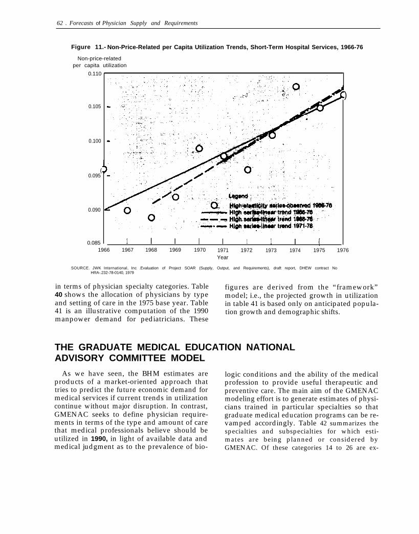
62 . Forecasts of Physician Supply and Requirements
Figure 11.- Non-Price-Related per Capita Utilization Trends, Short-Term Hospital Services, 1966-76
Non-price-relatedper capita utilization
0.110
0.105
0.100
(0.095
0.090
0.085 1 I I I I 1 1 I {
)
1966 1967 1968 1969 1970 1971 1972 1973 1974 1975 1976Year
SOURCE. JWK International, Inc .Evaluation of Project SOAR (Supply, Output, and Requirements), draft report, DHEW contract NoHRA-.232-78-0140, 1979
in terms of physician specialty categories. Table figures are derived from the “framework”40 shows the allocation of physicians by type model; i.e., the projected growth in utilizationand setting of care in the 1975 base year. Table in table 41 is based only on anticipated popula-41 is an illustrative computation of the 1990 tion growth and demographic shifts.manpower demand for pediatricians. These
THE GRADUATE MEDICAL EDUCATION NATIONALADVISORY COMMITTEE MODEL
As we have seen, the BHM estimates areproducts of a market-oriented approach thattries to predict the future economic demand formedical services if current trends in utilizationcontinue without major disruption. In contrast,GMENAC seeks to define physician require-ments in terms of the type and amount of carethat medical professionals believe should beutilized in 1990, in light of available data andmedical judgment as to the prevalence of bio-
logic conditions and the ability of the medicalprofession to provide useful therapeutic andpreventive care. The main aim of the GMENACmodeling effort is to generate estimates of physi-cians trained in particular specialties so thatgraduate medical education programs can be re-vamped accordingly. Table 42 summarizes thespecialties and subspecialties for which esti-mates are being planned or considered byGMENAC. Of these categories 14 to 26 are ex-
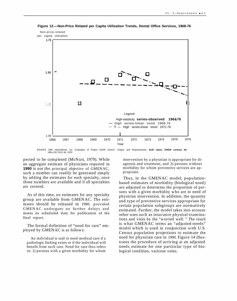
C h . 3 — R e q u i r e m e n t s ● 6 3
Figure 12.—Non-Price Related per Capita Utilization Trends, Dental Office Services, 1968-76
Non-pr ice-related
per capita utilization
1.75
1.50
1.25
1.00
13
Legend
High-elasticity series-observed 196&76--- High series-l inear trend 1968-76— 0 — High series-linear trend 1971-76
1
1966 1967 1968 1969 1970 1971 1972 1973 1974 1975 1976
Year
SOURCE JWK International. Inc. Evaluation of Project SOAR (Sum/Y. Output. and Requirements), draft report, DHEW contract NoHRA-232-78.01 40, 1979
pected to be completed (McNutt, 1979). Whilean aggregate estimate of physicians required in1990 is not the principal objective of GMENAC,such a number can readily be generated simplyby adding the estimates for each specialty, oncethose numbers are available and if all specialtiesare covered.
As of this time, no estimates for any specialtygroup are available from GMENAC. The esti-mates should be released in 1980, providedGMENAC undergoes no further delays andmeets its scheduled date for publication of thefinal report.
The formal definition of “need for care” em-ployed by GMENAC is as follows:
An individual is said to need medical care if apathologic finding exists or if the individual willbenefit from such care. Need for care thus refersto: 1) persons with a given morbidity for whom
intervention by a physician is appropriate for di-agnosis and treatment, and 2) persons withoutmorbidity for whom preventive services are ap-propriate.
Thus, in the GMENAC model, population-based estimates of morbidity (biological need)are adjusted to determine the proportion of per-sons with a given morbidity who are in need ofphysician intervention. In addition, the quantityand type of preventive services appropriate forcertain population subgroups are normativelyestimated. Further, the model takes into accountother uses such as insurance physical examina-tions and visits by the “worried well. ” The resultis what GMENAC terms an “adjusted-needs”model which is used in conjunction with U.S.Census population projections to estimate theneed for physician care in 1990. Figure 14 illus-trates the procedure of arriving at an adjustedneeds estimate for one particular type of bio-logical condition, varicose veins.
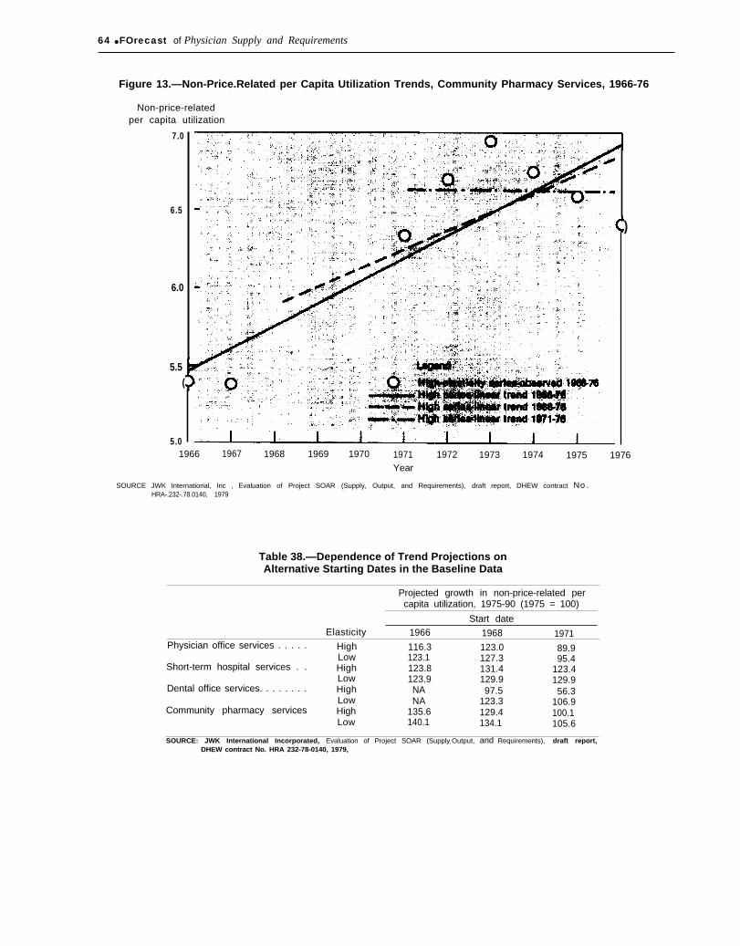
64 ● FOrecast of Physician Supply and Requirements
Figure 13.—Non-Price.Related per Capita Utilization Trends, Community Pharmacy Services, 1966-76
Non-price-relatedper capita utilization
7.0
6.5
6.0
5.5(
5.0
)
1966 1967 1968 1969 1970 1971 1972 1973 1974 1975 1976Year
SOURCE JWK International, Inc , Evaluation of Project SOAR (Supply, Output, and Requirements), draft report, DHEW contract No.HRA-.232-.78.0140, 1979
Table 38.—Dependence of Trend Projections onAlternative Starting Dates in the Baseline Data
Projected growth in non-price-related percapita utilization, 1975-90 (1975 = 100)
Start dateElasticity 1966 1968 1971
Physician office services . . . . . High 116.3 123.0 89.9Low 123.1 127.3 95.4
Short-term hospital services . . High 123.8 131.4 123.4Low 123.9 129.9 129.9
Dental office services. . . . . . . . High NA 97.5 56.3Low NA 123.3 106.9
Community pharmacy services High 135.6 129.4 100.1Low 140.1 134.1 105.6
SOURCE: JWK International Incorporated, Evaluation of Project SOAR (Supplyr Output, and Requirements), draft report,DHEW contract No. HRA 232-78-0140, 1979,
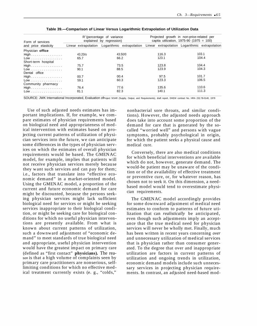
Ch. 3—Requirements ● 6 5
Table 39.—Comparison of Linear Versus Logarithmic Extrapolation of Utilization Data
R2 (percentage of variance Projected growth in non-price-related per
Form of services explained by regression) capita utilization, 1975-90 (1975 = 100)
and price elasticity Linear extrapolation Logarithmic extrapolation Linear extrapolation Logarithmic extrapolation
Physician officeHigh . . . . . . . . . . . . . . . . . 43.20/o 43.50/0 116.3 103.1Low . . . . . . . . . . . . . . . . . 65.7 66.2 123.1 104.4Short-term hospitalHigh . . . . . . . . . . . . . . . . . 75.7 73.5 123.8 104.4Low . . . . . . . . . . . . . . . . . 90.1 88.5 123.9 104.3Dental officeHigh . . . . . . . . . . . . . . . . . 00.7 00.4 97.5 101.7Low . . . . . . . . . . . . . . . . . 59.1 60.3 123.3 106.5Community pharmacyHigh . . . . . . . . . . . . . . . . . 76.4 77.6 135.6 110.6Low . . . . . . . . . . . . . . . . . 81.1 82.3 140.1 111.3
SOURCE: JWK International Incorporated, Evaluation of Project SOAR (Supply, Output, and Requirements), draft report, DHEW contract No. HRA 232.78-0140, 1979
Use of such adjusted needs estimates has im-portant implications. If, for example, we com-pare estimates of physician requirements basedon biological need and appropriateness of med-ical intervention with estimates based on pro-jecting current patterns of utilization of physi-cian services into the future, we can anticipatesome differences in the types of physician serv-ices on which the estimates of overall physicianrequirements would be based. The GMENACmodel, for example, implies that patients willnot receive physician services merely becausethey want such services and can pay for them;i.e., factors that translate into “effective eco-nomic demand” in a market-oriented model.Using the GMENAC model, a proportion of thecurrent and future economic demand for caremight be discounted, because the persons seek-ing physician services might lack sufficientbiological need for services or might be seekingservices inappropriate to their biological condi-tion, or might be seeking care for biological con-ditions for which no useful physician interven-tions are presently available. From what isknown about current patterns of utilization,such a downward adjustment of “economic de-mand” to meet standards of true biological needand appropriate, useful physician interventionwould have the greatest impact on primary care(defined as “first contact” physicians). The rea-son is that a high volume of complaints seen byprimary care practitioners are nonserious, self-limiting conditions for which no effective med-ical treatment currently exists (e. g., “colds,”
nonbacterial sore throats, and similar condi-tions). However, the adjusted needs approachdoes take into account some proportion of thedemand for care that is generated by the so-called “worried well” and persons with vaguesymptoms, probably psychological in origin,for which the patient seeks a physical cause andmedical cure.
Conversely, there are also medical conditionsfor which beneficial interventions are availablewhich do not, however, generate demand. Thewould-be patient may be unaware of the condi-tion or of the availability of effective treatmentor preventive cure, or, for whatever reason, haschosen not to seek it. On this dimension, a need-based model would tend to overestimate physi-cian requirements.
The GMENAC model accordingly providesfor some downward adjustment of medical needestimates to conform to patterns of future uti-lization that can realistically be anticipated,even though such adjustments imply an accept-ance that the true medical need for physicianservices will never be wholly met. Finally, muchhas been written in recent years concerning overand unnecessary utilization of medical servicesthat is physician rather than consumer gener-ated. To the degree that over and inappropriateutilization are factors in current patterns ofutilization and ongoing trends in utilization,economic demand models include such unneces-sary services in projecting physician require-ments. In contrast, an adjusted need-based mod-
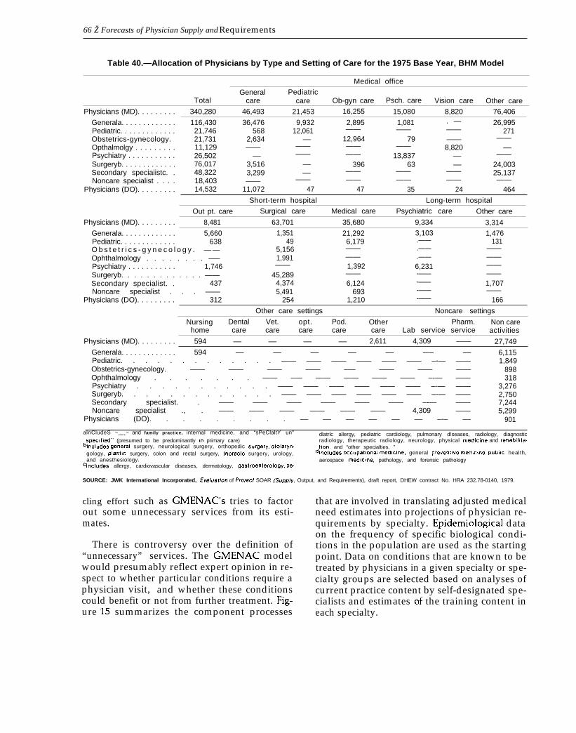
66 Ž Forecasts of Physician Supply and Requirements
Table 40.—Allocation of Physicians by Type and Setting of Care for the 1975 Base Year, BHM Model
Medical office
General PediatricTotal care care Ob-gyn care Psch. care Vision care Other care
Physicians (MD). . . . . . . . . 340,280 46,493 21,453 16,255 15,080 8,820 76,406
Generala. . . . . . . . . . . . . 116,430 36,476 9,932 2,895 1,081 . — 26,995Pediatric. . . . . . . . . . . . . 21,746 568 12,061 —— —— 271Obstetrics-gynecology.
——21,731 2,634 –– 12,964 79 ——
Opthalmolgy . . . . . . . . .——
11,129 —— —— —— —— 8,820 ––Psychiatry . . . . . . . . . . . 26,502 –– —— —— 13,837 ––Surgeryb. . . . . . . . . . . . .
——76,017 3,516 –– 396 63 –– 24,003
Secondary speciaiistc. . 48,322 3,299 –– —— —— 25,137Noncare specialist . . . .
——18,403 —— —— —— ——
Physicians (DO). . . . . . . . .—— ——
14,532 11,072 47 47 35 24 464
Short-term hospital Long-term hospital
Out pt. care Surgical care Medical care Psychiatric care Other care
Physicians (MD). . . . . . . . . 8,481 63,701 35,680 9,334 3,314
Generala. . . . . . . . . . . . . 5,660 1,351 21,292 3,103 1,476Pediatric. . . . . . . . . . . . . 638 49 6,179 131O b s t e t r i c s - g y n e c o l o g y . — —
.——5,156 —— .——
Ophthalmology . . . . . . . . –———
1,991 —— .——Psychiatry . . . . . . . . . . .
——1,746 —— 1,392 6,231
Surgeryb. . . . . . . . . . . . . ————
45,289 ——Secondary specialist. .
-—— ——437 4,374 6,124 -—— 1,707
Noncare specialist . . . —— 5,491 693Physicians (DO). . . . . . . . .
-—— ——312 254 1,210 -—— 166
Other care settings Noncare settings
Nursing Dental Vet. opt. Pod. Other Pharm. Non carehome care care care care care Lab service service activities
Physicians (MD). . . . . . . . . 594 –– –– –– –– 2,611 4,309 —— 27,749
Generala. . . . . . . . . . . . . 594 –– –– –– –– –– –-– –– 6,115Pediatric. . . . . . . . . . . . . —— —— —— —— —— —— –-— —— 1,849Obstetrics-gynecology. —— —— —— —— —– —— —— —— 898Ophthalmology . . . . . . . —— –— —— —— —— —— –-— —— 318Psychiatry . . . . . . . . . . . —— —— —— —— —— —— –-— —— 3,276Surgeryb. . . . . . . . . . . . . —— —— —— —— —— —— –-— —— 2,750Secondary specialist. . —— —— —— —— —— —— –-— —— 7,244Noncare specialist ., . —— —— —— —— —— —— 4,309 —— 5,299
Physicians (DO). . . . . . . . . –– –– –– –– –– –– –-– –– 901
alnCludeS ~enera ~ and family practice, internal medicine, and “sPeClaltY un” dlatrlc allergy, pediatric cardiology, pulmonary d!seases, radiology, diagnosticspeclfled” (presumed to be predominantly In primary care) radiology, therapeutic radiology, neurology, physical medlclne and rehablllta.
blncludes general surgery, neurological surgery, orthopedic sur9erY, otolarYn. tion, and “other specialties. ”gology, plastlc surgery, colon and rectal surgery, thoraclc surgery, urology, dlncludes occupatlona[ medlc!ne, general preventwe medlclne, publ!c health,and anesthesiology. aerospace medlclne, pathology, and forensic pathology
clncludes allergy, cardiovascular diseases, dermatology, 9aStrOenter0109Y, Pe-
SOURCE: JWK International Incorporated, Eva/uaffon of Pro/ect SOAR (SUpp/y, Output, and Requirements), draft report, DHEW contract No. HRA 232.78-0140, 1979.
cling effort such as GMENAC’S tries to factorout some unnecessary services from its esti-mates.
There is controversy over the definition of“unnecessary” services. The GMENAC modelwould presumably reflect expert opinion in re-spect to whether particular conditions require aphysician visit, and whether these conditionscould benefit or not from further treatment. Fig-
that are involved in translating adjusted medicalneed estimates into projections of physician re-quirements by specialty. Epidemiological dataon the frequency of specific biological condi-tions in the population are used as the startingpoint. Data on conditions that are known to betreated by physicians in a given specialty or spe-cialty groups are selected based on analyses ofcurrent practice content by self-designated spe-cialists and estimates of the training content in
ure 15 summarizes the component processes each specialty.
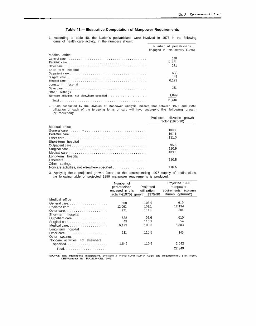
.
Table 41.— Illustrative Computation of Manpower Requirements
1. According to table 40, the Nation’s pediatricians were involved in 1975 in the followingforms of health care activity, in the numbers shown:
Number of pediatriciansengaged in this activity (1975)
Medical officeGeneral care. . . . . . . . . . . . . . . . . . . . . . . . . . . . . . . . . . . . . . . . . . .Pediatric care. . . . . . . . . . . . . . . . . . . . . . . . . . . . . . . . . . . . . . . . .Other care . . . . . . . . . . . . . . . . . . . . . . . . . . . . . . . . . . . . . . . . . . . .Short-term hospital .
Outpatient care . . . . . . . . . . . . . . . . . . . . . . . . . . . . . . . . . . . . . . . .Surgical care . . . . . . . . . . . . . . . . . . . . . . . . . . . . . . . . . . . . . . . . .Medical care. . . . . . . . . . . . . . . . . . . . . . . . . . . . . . . . . . . . . . . . . .Long.term hospitalOther care . . . . . . . . . . . . . . . . . . . . . . . . . . . . . . . . . . . . . . . . . . . .Other settingsNoncare activities, not elsewhere specified . . . . . . . . . . . . . . . .
56812,061
271
63849
6,179
131
1,849
Total . . . . . . . . . . . . . . . . . . . . . . . . . . . . . . . . . . . . . . . . . . . . . . . 21,746
2. Runs conducted by the Division of Manpower Analysis indicate that between 1975 and 1990,utilization of each of the foregoing forms of care will have undergone the following growth(or reduction):
Projected utilization growthfactor (1975-90)—
Medical office—
General care. . . . . . . . ~ . . . . . . . . . . . . . . . . . . . . . . . . . . . . . . . . . . 108.9Pediatric care. . . . . . . . . . . . . . . . . . . . . . . . . . . . . . . . . . . . . . . . . . 101.1Other care . . . . . . . . . . . . . . . . . . . . . . . . . . . . . . . . . . . . . . . . . . . . 111.0Short-term hospitalOutpatient care . . . . . . . . . . . . . . . . . . . . . . . . . . . . . . . . . . . . . . . . 95.6Surgical care . . . . . . . . . . . . . . . . . . . . . . . . . . . . . . . . . . . . . . . . . . 110.9Medical care. . . . . . . . . . . . . . . . . . . . . . . . . . . . . . . . . . . . . . . . . . 103.3Long-term hospitalOthercare . . . . . . . . . . . . . . . . . . . . . . . . . . . . . . . . . . . . . . . . . . . . 110.5Other settingsNoncare activities, not elsewhere specified . . . . . . . . . . . . . . . . 110.5
3. Applying these projected growth factors to the correspcmding 1975 supply of pediatricians,the following table of projected 1990 manpower requirements is produced:
Number of Projected 1990pediatricians Projected manpower
engaged in this utilization requirements (columnactivity(1975) growth, 1975-90 ltimes column2)— —
Medical officeGeneral care. . . . . . . . . . . . . . . . . . . . . 568 108.9 619Pediatric care. . . . . . . . . . . . . . . . . . . . 12,061 101.1 12,194Other care. . . . . . . . . . . . . . . . . . . . . . . 271 111.0 301Short-term hospitalOutpatient care . . . . . . . . . . . . . . . . . 638 95.6 610Surgical care. . . . . . . . . . . . . . . . . . . . . 49 110.9 54Medical care. . . . . . . . . . . . . . . . . . . . . 6,179 103.3 6,383Long-.term hospitalOther care. . . . . . . . . . . . . . . . . . . . . . . 131 110.5 145Other settingsNoncare activities, not elsewhere
specified. . . . . . . . . . . . . . . . . . . . 1,849 110.5 2,043
Total. . . . . . . . . . . . . . . . . . . . . . . . 22,349
SOURCE JWK International Incorporated. Evaluation of Pro/ecf SOAR (SuPP/Y Outpuf and RequlremefrfsL draft report.DHEWcontract No liRA232.78-Ol@. 1979
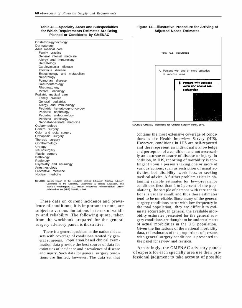
68 ● Forecasts of Physician Supply and Requirements
Table 42.—Specialty Areas and Subspecialtiesfor Which Requirements Estimates Are Being
Planned or Considered by GMENAC
Obstetrics-gynecologyDermatologyAdult medical care
Family practiceGeneral internal medicineAllergy and immunologyHematologyCardiovascular diseaseInfectious diseaseEndocrinology and metabolismNephrologyPulmonary diseaseGastroenterologyRheumatologyMedical oncology
Pediatric medical careFamily practiceGeneral pediatricsAllergy and immunologyPediatric hematology-oncologyPediatric nephrologyPediatric endocrinologyPediatric cardiologyNeonatal-perinatal medicine
OtolaryngologyGeneral surgeryColon and rectal surgeryOrthopedic surgeryThoracic surgeryOphthalmologyUrologyNeurosurgeryPlastic surgeryPathologyRadiologyPsychiatry and neurologyAnesthesiologyPreventive medicineNuclear medicine
SOURCE Interim Report o/ the Graduate Medical Education National AdvisoryCommittee to the Secretary, Department o/ Health, Education, andWe/fare, Washington, D.C. Health Resources Administration, DHEWpublication No (HRA) 79-633, p 206
These data on current incidence and preva-lence of conditions, it is important to note, aresubject to various limitations in terms of validi-ty and reliability. The following quote, takenfrom the workbook prepared for the generalsurgery advisory panel, is illustrative:
There is a general problem in the national datasets with coverage of conditions treated by gen-eral surgeons. Population based clinical exam-ination data provide the best source of data forestimates of incidence and prevalence of diseaseand injury. Such data for general surgery condi-tions are limited, however. The data set that
Figure 14.—lllustrative Procedure for Arriving atAdjusted Needs Estimates
Total U.S. population
A. Persons with one or more episodesof varicose veins
SOURCE GMENAC Workbook for General Surgery Panel, 1979.
contains the most extensive coverage of condi-tions is the Health Interview Survey (HIS).However, conditions in HIS are self-reportedand thus represent an individual’s knowledgeand perception of a condition, and not necessari-ly an accurate measure of disease or injury. Inaddition, in HIS, reporting of morbidity is con-tingent upon a person’s taking one or more ofvarious actions, such as restriction of usual ac-tivities, bed disability, work loss, or seekingmedical advice. A further problem exists in ob-taining reliable estimates for low-prevalenceconditions (less than 1 to 2 percent of the pop-ulation), The sample of persons with rare condi-tions is usually small, and thus these estimatestend to be unreliable. Since many of the generalsurgery conditions occur with low frequency inthe total population, they are difficult to esti-imate accurately. In general, the available mor-bidity estimates presented for the general sur-gery conditions are thought to be underestimatesof actual morbidities in the U.S. population.Given the limitations of the national morbiditydata, the estimates of the proportions of personswith general surgery conditions is presented tothe panel for review and revision.
Accordingly, the GMENAC advisory panelsof experts for each specialty area use their pro-fessional judgment to take account of possible
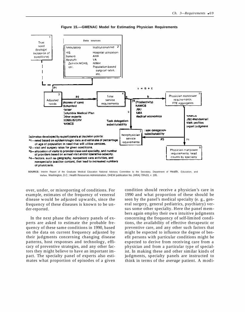
Ch. 3—Requirements ● 6 9
Figure 15.—GMENAC Model for Estimating Physician Requirements
III
I Data sources
P4
SOURCE: Interim Report of the Graduate Medical Education National Advisory Committee to the Secratary, Department of Health, Education, and
Wa/fare, Washington, D.C.: Health Resources Administration, DHEW publication No. (HRA) 79%33, P. 195.
over, under, or misreporting of conditions. Forexample, estimates of the frequency of venerealdisease would be adjusted upwards, since thefrequency of these diseases is known to be un-der-reported.
In the next phase the advisory panels of ex-perts are asked to estimate the probable fre-quency of these same conditions in 1990, basedon the data on current frequency adjusted bytheir judgments concerning changing diseasepatterns, host responses and technology, effi-cacy of preventive strategies, and any other fac-tors they might believe to have an important im-pact. The specialty panel of experts also esti-mates what proportion of episodes of a given
condition should receive a physician’s care in1990 and what proportion of these should beseen by the panel’s medical specialty (e. g., gen-eral surgery, general pediatrics, psychiatry) ver-sus some other specialty. Here the panel mem-bers again employ their own intuitive judgmentsconcerning the frequency of self-limited condi-tions, the availability of effective therapeutic orpreventive care, and any other such factors thatmight be expected to influence the degree of ben-efit persons with particular conditions might beexpected to derive from receiving care from aphysician and from a particular type of special-ist. In making these and other similar kinds ofjudgments, specialty panels are instructed tothink in terms of the average patient. A modi-
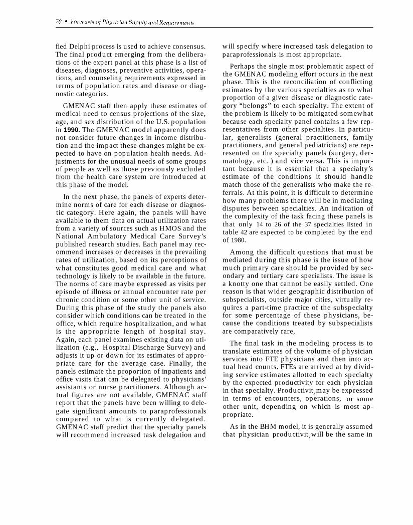
fied Delphi process is used to achieve consensus.The final product emerging from the delibera-tions of the expert panel at this phase is a list ofdiseases, diagnoses, preventive activities, opera-tions, and counseling requirements expressed interms of population rates and disease or diag-nostic categories.
GMENAC staff then apply these estimates ofmedical need to census projections of the size,age, and sex distribution of the U.S. populationin 1990. The GMENAC model apparently doesnot consider future changes in income distribu-tion and the impact these changes might be ex-pected to have on population health needs. Ad-justments for the unusual needs of some groupsof people as well as those previously excludedfrom the health care system are introduced atthis phase of the model.
In the next phase, the panels of experts deter-mine norms of care for each disease or diagnos-tic category. Here again, the panels will haveavailable to them data on actual utilization ratesfrom a variety of sources such as HMOS and theNational Ambulatory Medical Care Survey’spublished research studies. Each panel may rec-ommend increases or decreases in the prevailingrates of utilization, based on its perceptions ofwhat constitutes good medical care and whattechnology is likely to be available in the future.The norms of care maybe expressed as visits perepisode of illness or annual encounter rate perchronic condition or some other unit of service.During this phase of the study the panels alsoconsider which conditions can be treated in theoffice, which require hospitalization, and whatis the appropriate length of hospital stay.Again, each panel examines existing data on uti-lization (e.g., Hospital Discharge Survey) andadjusts it up or down for its estimates of appro-priate care for the average case. Finally, thepanels estimate the proportion of inpatients andoffice visits that can be delegated to physicians’assistants or nurse practitioners. Although ac-tual figures are not available, GMENAC staffreport that the panels have been willing to dele-gate significant amounts to paraprofessionalscompared to what is currently delegated.GMENAC staff predict that the specialty panelswill recommend increased task delegation and
will specify where increased task delegation toparaprofessionals is most appropriate.
Perhaps the single most problematic aspect ofthe GMENAC modeling effort occurs in the nextphase. This is the reconciliation of conflictingestimates by the various specialties as to whatproportion of a given disease or diagnostic cate-gory “belongs” to each specialty. The extent ofthe problem is likely to be mitigated somewhatbecause each specialty panel contains a few rep-resentatives from other specialties. In particu-lar, generalists (general practitioners, familypractitioners, and general pediatricians) are rep-resented on the specialty panels (surgery, der-matology, etc. ) and vice versa. This is impor-tant because it is essential that a specialty’sestimate of the conditions it should handlematch those of the generalists who make the re-ferrals. At this point, it is difficult to determinehow many problems there will be in mediatingdisputes between specialties. An indication ofthe complexity of the task facing these panels isthat only 14 to 26 of the 37 specialties listed intable 42 are expected to be completed by the endof 1980.
Among the difficult questions that must bemediated during this phase is the issue of howmuch primary care should be provided by sec-ondary and tertiary care specialists. The issue isa knotty one that cannot be easily settled. Onereason is that wider geographic distribution ofsubspecialists, outside major cities, virtually re-quires a part-time practice of the subspecialtyfor some percentage of these physicians, be-cause the conditions treated by subspecialistsare comparatively rare,
The final task in the modeling process is totranslate estimates of the volume of physicianservices into FTE physicians and then into ac-tual head counts. FTEs are arrived at by divid-ing service estimates allotted to each specialtyby the expected productivity for each physicianin that specialty. Productivity may be expressedin terms of encounters, operations, or someother unit, depending on which is most ap-propriate.
As in the BHM model, it is generally assumedthat physician productivity will be the same in
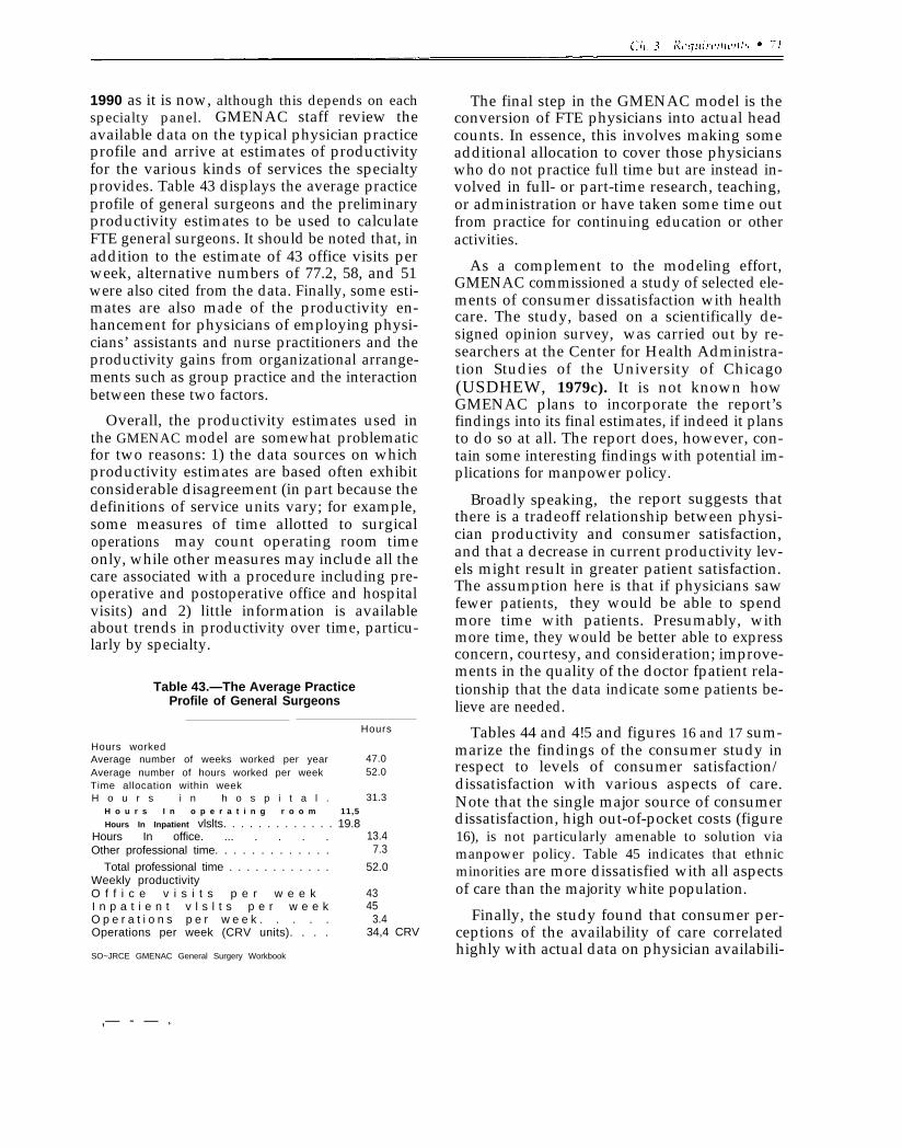
. — .
1990 as it is now, although this depends on eachspecialty panel. GMENAC staff review theavailable data on the typical physician practiceprofile and arrive at estimates of productivityfor the various kinds of services the specialtyprovides. Table 43 displays the average practiceprofile of general surgeons and the preliminaryproductivity estimates to be used to calculateFTE general surgeons. It should be noted that, inaddition to the estimate of 43 office visits perweek, alternative numbers of 77.2, 58, and 51were also cited from the data. Finally, some esti-mates are also made of the productivity en-hancement for physicians of employing physi-cians’ assistants and nurse practitioners and theproductivity gains from organizational arrange-ments such as group practice and the interactionbetween these two factors.
Overall, the productivity estimates used inthe GMENAC model are somewhat problematicfor two reasons: 1) the data sources on whichproductivity estimates are based often exhibitconsiderable disagreement (in part because thedefinitions of service units vary; for example,some measures of time allotted to surgicaloperations may count operating room timeonly, while other measures may include all thecare associated with a procedure including pre-operative and postoperative office and hospitalvisits) and 2) little information is availableabout trends in productivity over time, particu-larly by specialty.
Table 43.—The Average PracticeProfile of General Surgeons
Hours
Hours workedAverage number of weeks worked per year 47.0Average number of hours worked per week 52.0Time allocation within weekH o u r s i n h o s p i t a l . 31.3
H o u r s I n o p e r a t i n g r o o m 11,5
Hours In Inpatient vlslts. . . . . . . . . . . . . 19.8Hours In office. ... . . . . 13.4Other professional time. . . . . . . . . . . . . 7.3
Total professional time . . . . . . . . . . . . 52.0Weekly productivityO f f i c e v i s i t s p e r w e e k 43I n p a t i e n t v l s l t s p e r w e e k 45O p e r a t i o n s p e r w e e k . . . . . 3.4Operations per week (CRV units). . . . 34,4 CRV
SO~JRCE GMENAC General Surgery Workbook
The final step in the GMENAC model is theconversion of FTE physicians into actual headcounts. In essence, this involves making someadditional allocation to cover those physicianswho do not practice full time but are instead in-volved in full- or part-time research, teaching,or administration or have taken some time outfrom practice for continuing education or otheractivities.
As a complement to the modeling effort,GMENAC commissioned a study of selected ele-ments of consumer dissatisfaction with healthcare. The study, based on a scientifically de-signed opinion survey, was carried out by re-searchers at the Center for Health Administra-tion Studies of the University of Chicago(USDHEW, 1979c). It is not known howGMENAC plans to incorporate the report’sfindings into its final estimates, if indeed it plansto do so at all. The report does, however, con-tain some interesting findings with potential im-plications for manpower policy.
Broadly speaking, the report suggests thatthere is a tradeoff relationship between physi-cian productivity and consumer satisfaction,and that a decrease in current productivity lev-els might result in greater patient satisfaction.The assumption here is that if physicians sawfewer patients, they would be able to spendmore time with patients. Presumably, withmore time, they would be better able to expressconcern, courtesy, and consideration; improve-ments in the quality of the doctor fpatient rela-tionship that the data indicate some patients be-lieve are needed.
Tables 44 and 4!5 and figures 16 and 17 sum-marize the findings of the consumer study inrespect to levels of consumer satisfaction/dissatisfaction with various aspects of care.Note that the single major source of consumerdissatisfaction, high out-of-pocket costs (figure16), is not particularly amenable to solution viamanpower policy. Table 45 indicates that ethnicminorities are more dissatisfied with all aspectsof care than the majority white population.
Finally, the study found that consumer per-ceptions of the availability of care correlatedhighly with actual data on physician availabili-
,— - — 1-
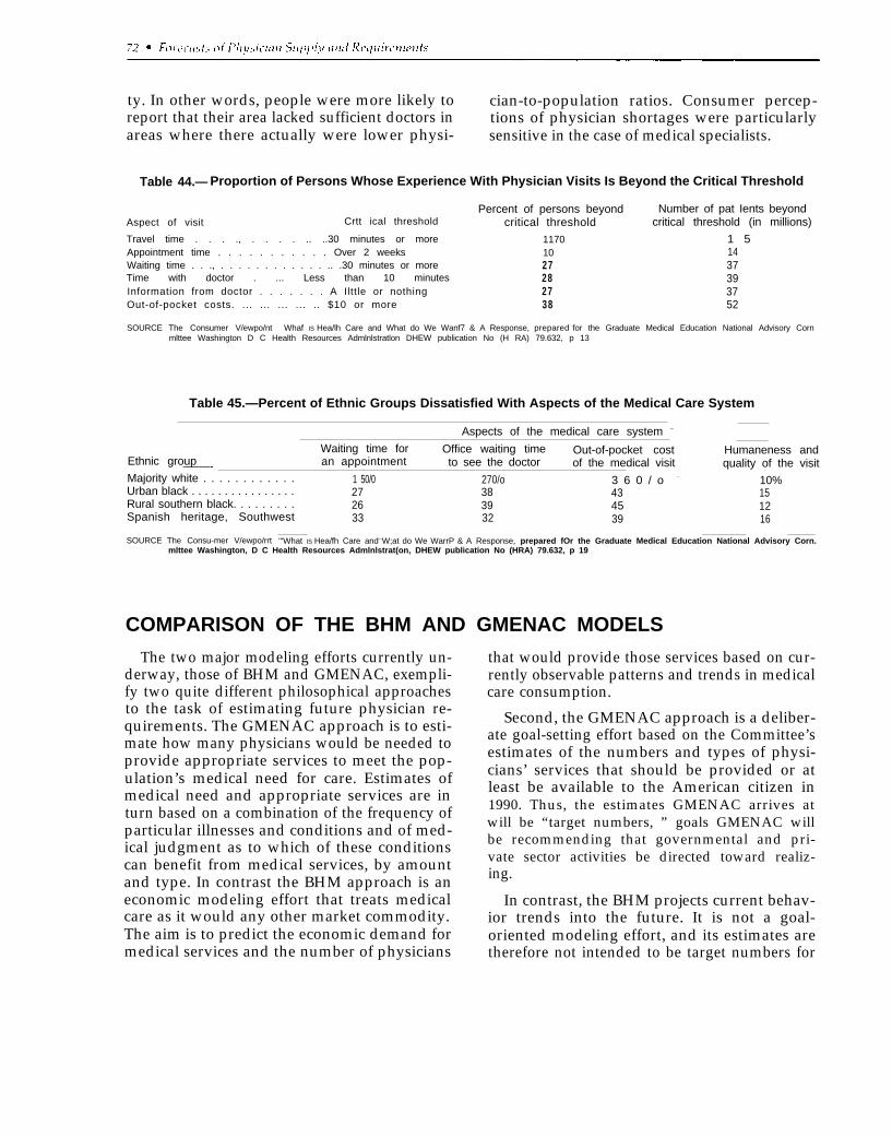
ty. In other words, people were more likely to cian-to-population ratios. Consumer percep-report that their area lacked sufficient doctors in tions of physician shortages were particularlyareas where there actually were lower physi- sensitive in the case of medical specialists.
Table 44.— Proportion of Persons Whose Experience With Physician Visits Is Beyond the Critical Threshold
Aspect of visit Crtt ical threshold
Travel time . . . ., . . . . .. ..30 minutes or moreAppointment time . . . . . . . . . . . Over 2 weeksWaiting time . . ., . . . . . . . . . . . . .. .30 minutes or moreTime with doctor . ... Less than 10 minutesInformation from doctor . . . . . . . A Ilttle or nothingOut-of-pocket costs. ... ... ... ... .. $10 or more
Percent of persons beyondcritical threshold
11701027282738
Number of pat Ients beyondcritical threshold (in millions)
1 51437393752
SOURCE The Consumer V/ewpo/nt Whaf IS Hea/lh Care and What do We Wanf7 & A Response, prepared - for the Graduate Medical Education National Advisory Cornmlttee Washington D C Health Resources Admlnlstratlon DHEW publication No (H RA) 79.632, p 13
Table 45.—Percent of Ethnic Groups Dissatisfied With Aspects of the Medical Care System
Aspects of the medical care system –
Waiting time for Office waiting time Out-of-pocket cost Humaneness andEthnic group an appointment to see the doctor of the medical visit quality of the visit———-Majority white . . . . . . . . . . . . 1 50/0 270/o 3 6 0 / o - 10%Urban black . . . . . . . . . . . . . . . . 27 38 43 15Rural southern black. . . . . . . . . 26 39 45 12Spanish heritage, Southwest 33 32 39 16
SOURCE The Consu-mer V/ewpo/rrt ‘“What IS Hea/fh Care and—W;at do We WarrP & A Response, prepared fOr the Graduate Medical Education National Advisory Corn.mlttee Washington, D C Health Resources Admlnlstrat(on, DHEW publication No (HRA) 79.632, p 19
COMPARISON OF THE BHM AND GMENAC MODELS
The two major modeling efforts currently un-derway, those of BHM and GMENAC, exempli-fy two quite different philosophical approachesto the task of estimating future physician re-quirements. The GMENAC approach is to esti-mate how many physicians would be needed toprovide appropriate services to meet the pop-ulation’s medical need for care. Estimates ofmedical need and appropriate services are inturn based on a combination of the frequency ofparticular illnesses and conditions and of med-ical judgment as to which of these conditionscan benefit from medical services, by amountand type. In contrast the BHM approach is aneconomic modeling effort that treats medicalcare as it would any other market commodity.The aim is to predict the economic demand formedical services and the number of physicians
that would provide those services based on cur-rently observable patterns and trends in medicalcare consumption.
Second, the GMENAC approach is a deliber-ate goal-setting effort based on the Committee’sestimates of the numbers and types of physi-cians’ services that should be provided or atleast be available to the American citizen in1990. Thus, the estimates GMENAC arrives atwill be “target numbers, ” goals GMENAC willbe recommending that governmental and pri-vate sector activities be directed toward realiz-ing.
In contrast, the BHM projects current behav-ior trends into the future. It is not a goal-oriented modeling effort, and its estimates aretherefore not intended to be target numbers for
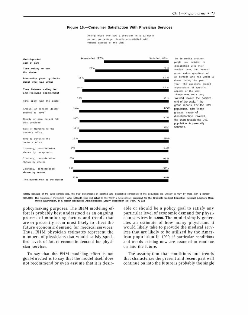
Figure 16.—Consumer Satisfaction With Physician Services
Out-of-pocket
cost of care
Time waiting to see
the doctor
Information given by doctor
about what was wrong
Time between calling for
and receiving appointment
Time spent with the doctor
Amount o f concern doctor
seemed to have
Quality of care patient felt
was provided
Cost of traveling to the
doctor ’s o f f ice
Time to travel to the
doctor ’s o f f ice
Cour tesy, cons iderat ion
shown by recept ion is t
Cour tesy, cons iderat ion
shown by doctor
Cour tesy, cons iderat ion
shown by nurses
The overall visit to the doctor
Among those who saw a physician in a 12-month
per iod, percentage d issat is f ied /sat is f ied wi th
various aspects of the visit.
Dissatisfied 3 7 % Sat is f ied 63%
28“A 72 %
18’-’/0 82 %
1 6 0 / 0 8 4 0 / 0
16% 84 “/o
130/o 87°10
13% 8 7 %
13 “/0 870/0
12 % 880/0
9% 91%
8% 92 %
7 0/0 93° 0
12% 8 8 %
To determine whether
people are satisfied or
d issat is f ied wi th the i r
medical care, the research
group asked quest ions of
all persons who had visited a
doctor during the past
year. The questions probed
impress ions o f spec i f ic
aspects of the visit.
“Responses were very
skewed toward the positiveend of the scale, ” thegroup reports, For the totalpopulation, cost iS thegreatest cause ofdissatisfaction Overall,the chart reveals the U.S.population iS genera//ysatisfied.
NOTE Because of the large sample size, the true’ percentages of satisfied and dissatisfied consumers in the population are unlikely to vary by more than 1 percent
SOURCE The Consumer Viewpoint ‘ What iS Health Care and What do We Want” & A Response, prepared for the Graduate Medical Education National Advisory Cornmittee Washington, D C Health Resources Administration, DHEW publication No (HRA) 79-632
policymaking purposes. The BHM modeling ef- able or should be a policy goal to satisfy anyfort is probably best understood as an ongoing particular level of economic demand for physi-process of monitoring factors and trends that cian services in 1.990. The model simply gener-are or presently seem most likely to affect the ates an estimate of how many physicians itfuture economic demand for medical services. would likely take to provide the medical serv-Thus, BHM physician estimates represent the ices that are likeIy to be utilized by the Amer-numbers of physicians that would satisfy speci- ican population in 1990, if particular conditionsfied levels of future economic demand for physi- and trends existing now are assumed to continuecian services. on into the future.
To say that the BHM modeling effort is not The assumption that conditions and trendsgoal-directed is to say that the model itself does that characterize the present and recent past willnot recommend or even assume that it is desir- continue on into the future is probably the single
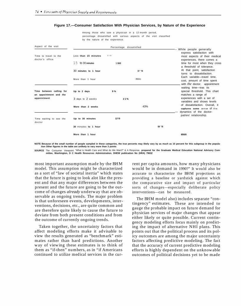
Figure 17.—Consumer Satisfaction With Physician Services, by Nature of the Experience
Aspect of the visit
Time to travel to the
doctor ’s o f f ice
Time between calling for
an appointment and the
appointment
Time waiting to see the
doc to r
Among those who saw a physician in a 12-month period,
percentage dissatisfied with various aspects of the visit classified
by the nature of the experience.
Percentage d issat is f ied— While people generally
express satisfaction withLess than 15 minutes 4 “ / 0 most aspects of their medical
experiences, there comes a15 to 30 minutes 1 30/0 time for most when they cross
a threshold of tolerance.
30 minutes to 1 hour 37 ”/0 At that point, satisfactionturns to dissatisfaction.
More than 1 hour 350/oEach variable—travel time,cost, amount of time spentwith the doctor, appointmentwaiting time—tras its
Up to 2 days 9 % special threshold. This chartmatches a range of
3 days to 2 weeks 2 1 % experiences with a set ofvariables and shows levels
More than 2 weeks 43% of dissatisfaction. Overall, itcaptures some sense of t h e
— dynamics of the doctor-
Up to 30 minutes 13“/0pat/en/ relationship.
30 minutes to 1 hour 59 ”/0
More than 1 hour 850/0
NOTE Because of the small number of people sampled in these categories, the true percents may Iikely vary by as much as 10 percent for this subgroup in the popula-tion Other figures in the table are unlikely to vary more than 3 points
SOURCE The Consumer Viewpoint “What is Health Care and What do We Want?” & A Response, prepared for the Graduate Medical Education National Advisory Com-mittee, Washington, D C Health Resources Administration. DHEW publication No (HRA) 79632
most important assumption made by the BHMmodel. This assumption might be characterizedas a sort of “law of societal inertia” which statesthat the future is going to look alot like the pres-ent and that any major differences between thepresent and the future are going to be the out-come of changes already underway that are ob-servable as ongoing trends. The major problemis that unforeseen events, developments, inter-ventions, decisions, etc., are quite common andare therefore quite likely to cause the future todeviate from both present conditions and fromthe outcome of currently ongoing trends.
Taken together, the uncertainty factors thataffect modeling efforts make it advisable toview the results generated as “benchmark” esti-mates rather than hard predictions. Anotherway of viewing these estimates is to think ofthem as “if-then” numbers, as in “if Americanscontinued to utilize medical services in the cur-
rent per capita amounts, how many physicianswould be in demand in 1990?” It would also beaccurate to characterize the BHM projections asproviding a baseline or yardstick against whichthe comparative size and impact of particularsorts of changes—especially deliberate policyinterventions—can be measured.
The BHM model also) includes separate “con-tingency” estimates. These are intended togauge the probable impact on future demand forphysician services of major changes that appeareither likely or quite possible. Current contin-gency modeling efforts focus mainly on predict-ing the impact of alternative NHI plans. Thispoints out that the political process and its pol-icy outcomes are among the major uncertaintyfactors affecting predictive modeling. The factthat the accuracy of current predictive modelingefforts is highly dependent on the unknowableoutcomes of political decisions yet to be made
simply underscores the point made earlier thatthese estimates should be viewed as “bench-mark” or baseline estimates.
As a goal-directed modeling effort,GMENAC’S most important core assumptionsare that reasonable estimates of appropriateutilization of medical services and the numbersand types of physicians needed to provide thoseservices can be derived from a combination ofempirical data and professional judgment con-cerning “medical need. ” The standard of med-ical need being applied to the determination ofappropriate utilization of services requires asomewhat stronger presumption of linkage be-tween medical service and improvements inhealth outcome than a standard based on a vol-ume of services provided, not because they areexpected to produce beneficial effects in most in-stances, but because in some instances theymight yield improvements and in the rest ofcases are believed to do no harm. The standardbeing used would tend to be more conservativein estimating the medical need for such margin-ally beneficial services, especially where themedical problem or illness is a nonserious con-dition.
An illustration of how this theoretical dif-ference translates into practice can be seen in thedeliberations of GMENAC’S dermatology panelon the treatment of acne. In its first round, thepanel’s initial estimate of medical need assumedthat every case of acne should be seen by a der-matologist, and that a typical case would re-quire six visits annually (which assumes medica-tion and the need to monitor its effects). Insubsequent rounds of discussion, however, thepanel determined that this number was exces-sive and revised their initial estimate downwardto reflect a more conservative definition of need.In lowering their original estimate of need fordermatologists to treat acne, the panel took intoaccount such factors as the nonserious, self-limiting character of a high proportion of acnecases, the fact that medical treatment is mostlikely to produce improvement in severe casesand, finally, the fact that nonserious cases ofacne can be treated as safely and efficaciouslyby appropriately trained generalists as by spe-cialists in dermatology.
As a goal-directed model more concernedwith defining what should be rather than fore-casting what is likely to be, the GMENAC effortneed not be as concerned with the problemsposed by uncertainty factors as the BHM trendprojection and contingency models must be. It isalso relevant that the goals being formulated arefor the comparative near-term future. Thus,GMENAC’S definitions of medical need arebased on the assumptions: 1) that Americanswill continue to have the same medical prob-lems at the same demographic (e.g., age, sex,social class) rates in 1990 as they do now, and 2)that there will be no major breakthroughs inmedical knowledge or technology that will seri-ously alter current medical practice. While theseassumptions are probably reasonable for a peri-od covering little over a decade, they might wellbecome more doubtful if the time span were ex-panded.
More problematic for a near-term, goal-di-rected model than the uncertainties of the futureare the reality constraints of the past and pres-ent. What we mean by this is that societies arenot like marching bands: policy makers cannotblow the whistle and expect society (or one of itsmajor subunits such as the health system) to ex-ecute a 90-degree turn in formation. Yet in asense that is what efforts to establish andachieve collective goals frequently assume canbe accomplished. Clearly, the more greatly agoal-directed estimate differs from anticipatedsupply and the shorter the time period avail-able, the more we must implicitly assume that90-degree societal pivots are possible; at least ifthe goal is taken seriously as one we ought to tryto achieve.
A much more serious reality constraint is thatthere may be insufficient “play” or “slack” in thesystem to permit actual attainment of a physi-cian “requirements” estimate that deviates dras-tically from the currently projected 1990 supply.At issue is what policy researchers term the rela-tive “malleability” of key variables. The possi-bility of attaining a goal within a given period oftime is dependent on the malleability of supplyfactors. Supply factors, however, are not highlymalleable. The reason for this is, that, as 1990 isonly 10 years away and physician training re-
quires a long Ieadtime, most of the 1990 supplyis already locked in. And even though 40 per-cent of the physicians in practice in 1990 willhave completed training since 1979 (Jacoby,1980), major changes in graduate medical edu-cation cannot be expected to take place andhave a significant impact on the specialty distri-bution of the 1990 physician supply. Perhaps fu-ture goal-oriented modeling efforts should payexplicit attention to the relative “malleability”of key variables. In so doing, they might pro-vide alternative estimates, signaling, on the onehand, goals that are capable of attainment with-in the allotted time span and, on the other hand,goals that are considered desirable but would re-quire a longer time frame and are thus best con-sidered as signaling the appropriate direction fordeliberate change but not taken as immediatetargets.
So far we have discussed only one set of reali-ty constraints (i.e., limitations on the mallea-bility of the health manpower supply) that im-pinges on the feasibility of a goal-orientedmodel of physician requirements. There areother factors as well. One is the difference be-tween the types of conditions that ought to beseen by particular types of physicians and actualpatterns of physician use. For example, a non-trivial portion of the current caseload of gener-alist physicians is composed of nonserious, self-limiting conditions that medical treatment cando little to cure or ameliorate (e.g., “colds”).These cases would tend to be discounted basedstrictly on medical need. There is little reason toexpect however, that, in reality, patients wouldrapidly be reoriented to stop bringing such com-plaints to physicians or that physicians wouldrefuse to see patients with such complaints.Thus, GMENAC’S normative model accountsfor some need to provide services to the “wor-ried well, ” and the BHM estimates include pres-ent use of medical services by the “worried well”in its projections.
The need to pay attention to both goals andreality leads naturally to a consideration of thecomplementarily of goal-driven and trend pro-jection modeling. Because each of these two ma-jor modeling efforts is oriented toward differentpurposes and focuses on rather different vari-
ables, they are, in truth, more complementarythan competing. As such, each model’s resultscan aid our interpretation of the other’s.
The GMENAC model focuses on translating anormative definition of medical need into ap-propriate rates of utilization of medical services,while the BHM model looks on medical care as a“consumer good” and treats empirical trends inutilization of medical services as a proxy foreconomic demand. If the BHM demand esti-mates should prove significantly greater thanthe GMENAC estimates, this would suggest thatthere are powerful factors at work that arepushing utilization of medical services beyondthe level medically necessary and appropriatefor “good” care. This would then raise thepolicy question of what percentage—if any—ofthe projected future economic demand for medi-cal services over and above the professionaljudgment-based estimates of medical n e e dshould be considered legitimate. Conversely, ifthe BHM demand estimates should prove sig-nificantly less than the GMENAC estimates, thiswould suggest that there remain and will remainin the near future significant barriers to obtain-ing medically necessary care. Finally, if theBHM and GMENAC demand estimates prove tobe in rough parity, this would suggest that theeconomic demand for services is more or less inline with professional estimates of the medicalneed for physician services.
Obviously, since the GMENAC model hasyet to generate any numbers, it is impossible tosay at the present time which of these threealternatives will prove to be the case. We cansay, however, that the most likely occurrencewould appear to be rough parity or a BHM de-mand estimate that is significantly greater thanthe GMENAC aggregate estimate. The majorreason for anticipating that the BHM estimatewill most likely prove greater than or at leastequal to the GMENAC estimate is that one ofthe major variables in the BHM model is a pro-jected trend toward rising per capita utilizationrates for medical services, independent of demo-graphic changes and projected changes in price.In contrast, the GMENAC model assumes nomajor changes in medical need apart fromchanges in medical need induced by demograph-
ic shifts (e. g., an aging population), betweennow and 1990; hence no medical rationale forsteadily rising per capita utilization of services.Thus, in order for the GMENAC estimate tologically come out larger than the BHM esti-mate, one would need to assume that there iscurretztly such a large unmet medical need forservices, that, despite the trend of rising percapita utilization rates, assumed in the BHMmodel, considerable unmet medical need will re-main in 1990.
What is a reasonable estimate of requirementsfrom the BHM economic model which might ap-proximate aggregate adjusted need from theGMENAC modeling effort? Recall that BHMnow projects demand at approximately 600,000physicians in 1990, or what the supply will be.We saw (table 37) that this represented an in-crease of 217,841 over the 1975 figure of378,376; 35,960 was due to an increasing andchanging population, and 181,881 due to pro-jected increases in per capita utilization trends.That is, without increasing per capita utiliza-tion, demand in 1990 would be roughly415,000.
We also saw (figures 10 through 13) that thelarge increase attributed to rising per capitautilization would nearly disappear if pre-1970’sdata were deleted from the trend base. But wewould not want to discount this increase entire-ly for several reasons: 1) the possibility of NHI,2) possible decreases in the average physician’s
PRODUCTIVITY
Both BHM’s and GMENAC’S modeling ef-forts emphasize the amount of medical servicesthat either will (based on predictions of trends)or should (based on normative determinationsof medical need) be used in the future. However,estimates of the number of physicians requiredare derived by dividing projected use by physi-cian productivity. With the exception of taskdelegation to physicians’ assistants and nursepractitioners, which would enhance physicianproductivity and thereby reduce aggregate phy-sician requirements, neither modeling effort ex-plores possible changes in productivity and theireffects on requirements estimates. Rather, both
workweek, and 3) increasing the time physi-cians spend with patients.
The possible effects of an NHI program havepreviously been summarized. Physicians cur-rently average longer workweeks than most ofthe rest of the working population. Bringing thephysician workweek more into line with thepresent patterns of work productivity of thelabor force in general would lower productivity.Alternatively, the cushion of excess physiciansmight enable physicians to see fewer patientsand spend more time with each one. Accordingto the National Center for Health Statistics,about half of all office visits to physicians inboth 1973 and 1977 lasted 10 minutes or less.With smaller patient loads, doctors might beable to use the additional time to provide pa-tients with more information, education, andcounseling.
For these reasons, it is difficult to estimatephysician requirements. If one takes projectedpopulation changes alone, requirements in thismodel would be for 415,000 physicians. Somecontingency is necessary to account for such fac-tors as NHI, decreased working hours for physi-cians, and more time spent with patients pervisit. How much of a contingency is necessary isa matter of judgment, and the reader can cometo his or her own conclusion on what it shouldbe over and above the increase in requirementsdue to population growth.
models basically assume that physician produc-tivity will remain constant through 1990. TheBHM model does this by assuming that the ratioof practicing physicians to total output of physi-cian services will be the same in 1990 as it was in197.s. In the case of GMENAC, the main efforthas been toward choosing the most reliable andaccurate measures of current productivity as re-flected in various empirical studies, Its modelingeffort makes explicit assumptions about theaverage workweek, patient visit rates, etc., byeach medical specialty.
But physician requirements estimates arehighly sensitive to changes in productivity
(Reinhardt, 1975). As an illustration of this sen-sitivity, if we were to postulate that the appro-priate ratio of physicians-to-population in 1970was 185 per 100,000 (the actual ratio in the best-endowed areas) and percent growth in produc-tivity kept pace with percent growth in per capi-ta use of physician services, then the physician-to-population ratio would remain constant in-definitely. However, as Reinhardt points out:
If in 1970 a set of policies could have been im-plemented such that average annual growth inphysician productivity during the following twodecades were one percentage point higher thanthe annual growth in the per capita utilization ofphysician services, then the required ratio at theend of the forecast horizon would have beenonly 151 physicians per 100,000. Relative to aforecast based on maintenance of the base-yearratio of 185 per 100,000 and for a population ofroughly 250 million in 1990, this turn of eventswould have led to a reduction of about 85,000 inthe number of MDs that would otherwise havebeen “required.” The corresponding number for1980, based on a projected population of 225million, is 40,500. These figures must surelystrike one as significant, especially if held upagainst the annual number of medical graduates(between 15,000 and 16,000) likely to be pro-duced during the next several decades (Rein-hardt, 1975).
Reinhardt’s analysis was primarily concernedwith the impact of substantial gains in produc-tivity that might occur as a result of organiza-tional changes in physicians’ practices and oftask delegation to nurse practitioners and physi-cians’ assistants. His research also providessome data suggestive of a possible relationshipbetween growth in physician supply and de-creases in physician productivity. Table 46 (re-produced from Reinhardt, 1975) provides somedata on relationships between physician supply,physician productivity, and financial factorssuch as average visit fee and average annualphysician income. If physician supply increases(item #l) but demand for services (per capitause) remains constant (item W), then produc-tivity (measured in patient visits per MD) willdrop (item #3). The data suggest that physiciansthen may charge more per visit (item #7),though not necessarily enough for physicians’incomes to reach the same level as in areas with
fewer physicians and/or greater demand forservices (item #8).
A different approach to the question of physi-cian productivity and its relationship to require-ments estimates is to examine trends in physi-cian productivity. According to Medical Eco-nomics magazine’s Continuing Survey, compar-ing workweeks in 1965 versus 1976, office-basedphysicians spent 2 hours less with office pa-tients, 2 hours less on housecalls, and 1 hour lesson hospital rounds and consultations in 1976.Median time spent on all professional activities(including activities other than patient care) in atypical workweek fell from 64 hours in 1965 to60 hours in 1976 (Owens, 1977).
More recently, Medical Economics reportedthat the number of office visits has continued todecline. Over the period 1974-78, office-basedphysicians were seeing 8 fewer patients per weekin 1978 as compared to 1974, a median weeklynumber of 126 rather than 134 (Owens, 1979).
Generally, two hypotheses are given to ex-plain recent decreases in productivity and topredict further decreases. One hypothesis is thatphysicians, as most other Americans, wouldprefer to work less and enjoy more leisure time.The other hypothesis is if growth in physiciansupply outpaces growth in the demand for phy-sician services, then declines in physician pro-ductivity may occur as a means of bringing sup-ply and demand into balance.
In the latest survey (Owens, 1979) 57 percentof the office-based physicians stated that theybelieved they were practicing at full capacity.Of this 57 percent, a minority (amounting to 12percent of the entire sample of physicians sur-veyed) said they would prefer not to practice atpeak productivity. Of those surveyed 43 percentsaid that they were not practicing at peak pro-ductivity. Of these, a majority said they did notwant to practice at full capacity. Of the entiresample 18 percent, however, stated that theywere not practicing at full capacity but wouldprefer to do so. Among the specialties, 31 per-cent of urologists, 24 percent of general sur-geons, and 24 percent of otolaryngologists saidthat they were not practicing at peak productivi-ty and would prefer to do so.
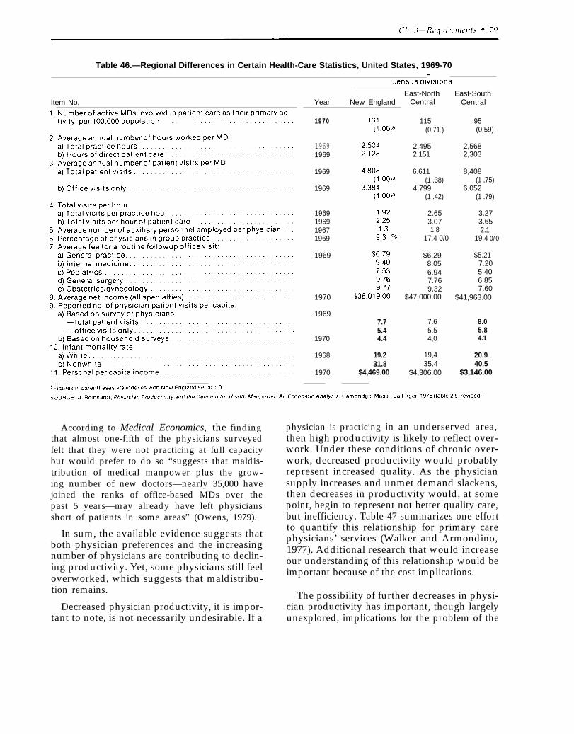
Table 46.—Regional Differences in Certain Health-Care Statistics, United States, 1969-70—
Item No.East-North
Year New England
1970
19691969
1969
1969
1969196919671969
1969
1970
1969
1970
1968
1970
7.75.44.4
19.231.8
$4,469.00
Central
115(0.71 )
2,4952.151
6.611(1 .38)
4,799(1 .42)
2.653.071.8
17.4 0/0
$6.298.056.947.769.32
$47,000.00
7.65.54,0
19,435.4
$4,306.00
East-SouthCentral
95(0.59)
2,5682,303
8,408(1 ,75)
6.052(1 .79)
3.273.652.1
19.4 0/0
$5.217.205.406.857.60
$41,963.00
8.05.84.1
20.940.5
$3,146.00
According to Medical Economics, the findingthat almost one-fifth of the physicians surveyedfelt that they were not practicing at full capacitybut would prefer to do so “suggests that maldis-tribution of medical manpower plus the grow-ing number of new doctors—nearly 35,000 havejoined the ranks of office-based MDs over thepast 5 years—may already have left physiciansshort of patients in some areas” (Owens, 1979).
In sum, the available evidence suggests thatboth physician preferences and the increasingnumber of physicians are contributing to declin-ing productivity. Yet, some physicians still feeloverworked, which suggests that maldistribu-tion remains.
Decreased physician productivity, it is impor-tant to note, is not necessarily undesirable. If a
physician is practicing in an underserved area,then high productivity is likely to reflect over-work. Under these conditions of chronic over-work, decreased productivity would probablyrepresent increased quality. As the physiciansupply increases and unmet demand slackens,then decreases in productivity would, at somepoint, begin to represent not better quality care,but inefficiency. Table 47 summarizes one effortto quantify this relationship for primary carephysicians’ services (Walker and Armondino,1977). Additional research that would increaseour understanding of this relationship would beimportant because of the cost implications.
The possibility of further decreases in physi-cian productivity has important, though largelyunexplored, implications for the problem of the
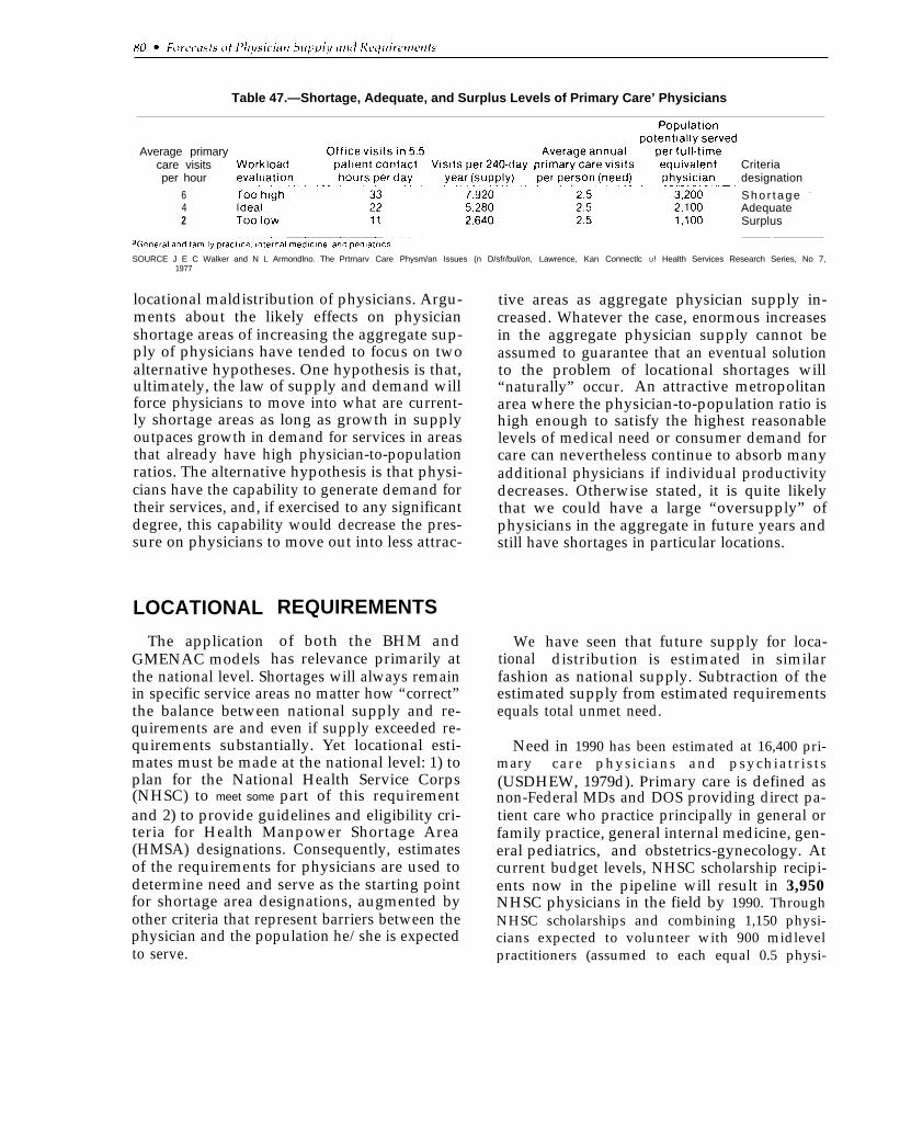
Table 47.—Shortage, Adequate, and Surplus Levels of Primary Care’ Physicians
Average primarycare visitsper hour
642
Criteriadesignation
S h o r t a g e -
AdequateSurplus
SOURCE J E C Walker and N L Armondlno. The Prtrnarv Care Physm/an Issues (n D/sfr/bul/on, Lawrence, Kan Connectlc U! Health Services Research Series, No 7,1977
locational maldistribution of physicians. Argu-ments about the likely effects on physicianshortage areas of increasing the aggregate sup-ply of physicians have tended to focus on twoalternative hypotheses. One hypothesis is that,ultimately, the law of supply and demand willforce physicians to move into what are current-ly shortage areas as long as growth in supplyoutpaces growth in demand for services in areasthat already have high physician-to-populationratios. The alternative hypothesis is that physi-cians have the capability to generate demand fortheir services, and, if exercised to any significantdegree, this capability would decrease the pres-sure on physicians to move out into less attrac-
LOCATIONAL
The applicationGMENAC models
REQUIREMENTS
of both the BHM andhas relevance primarily at
the national level. Shortages will always remainin specific service areas no matter how “correct”the balance between national supply and re-quirements are and even if supply exceeded re-quirements substantially. Yet locational esti-mates must be made at the national level: 1) toplan for the National Health Service Corps(NHSC) to meet some part of this requirementand 2) to provide guidelines and eligibility cri-teria for Health Manpower Shortage Area(HMSA) designations. Consequently, estimatesof the requirements for physicians are used todetermine need and serve as the starting pointfor shortage area designations, augmented byother criteria that represent barriers between thephysician and the population he/she is expectedto serve.
tive areas as aggregate physician supply in-creased. Whatever the case, enormous increasesin the aggregate physician supply cannot beassumed to guarantee that an eventual solutionto the problem of locational shortages will“naturally” occur. An attractive metropolitanarea where the physician-to-population ratio ishigh enough to satisfy the highest reasonablelevels of medical need or consumer demand forcare can nevertheless continue to absorb manyadditional physicians if individual productivitydecreases. Otherwise stated, it is quite likelythat we could have a large “oversupply” ofphysicians in the aggregate in future years andstill have shortages in particular locations.
Wetional
have seen that future supply for loca-distribution is estimated in similar
fashion as national supply. Subtraction of theestimated supply from estimated requirementsequals total unmet need.
Need in 1990 has been estimated at 16,400 pri-mary care physicians and psychiatrists(USDHEW, 1979d). Primary care is defined asnon-Federal MDs and DOS providing direct pa-tient care who practice principally in general orfamily practice, general internal medicine, gen-eral pediatrics, and obstetrics-gynecology. Atcurrent budget levels, NHSC scholarship recipi-ents now in the pipeline will result in 3,950NHSC physicians in the field by 1990. ThroughNHSC scholarships and combining 1,150 physi-cians expected to volunteer with 900 midlevelpractitioners (assumed to each equal 0.5 physi-
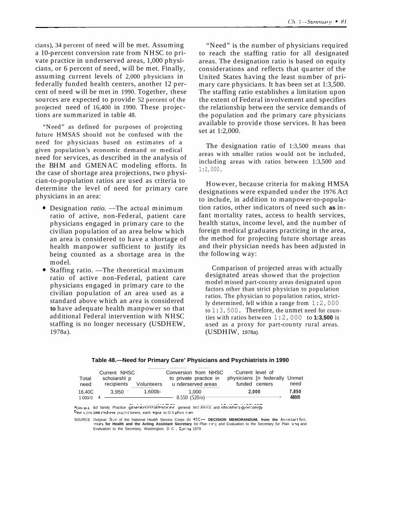
cians), 34 percent of need will be met. Assuminga 10-percent conversion rate from NHSC to pri-vate practice in underserved areas, 1,000 physi-cians, or 6 percent of need, will be met. Finally,assuming current levels of 2,000 physicians infederally funded health centers, another 12 per-cent of need will be met in 1990. Together, thesesources are expected to provide 52 percent of theprojected need of 16,400 in 1990. These projec-tions are summarized in table 48.
“Need” as defined for purposes of projectingfuture HMSAS should not be confused with theneed for physicians based on estimates of agiven population’s economic demand or medicalneed for services, as described in the analysis ofthe BHM and GMENAC modeling efforts. Inthe case of shortage area projections, two physi-cian-to-population ratios are used as criteria todetermine the level of need for primary carephysicians in an area:
●
●
Designation ratio. —The actual minimumratio of active, non-Federal, patient carephysicians engaged in primary care to thecivilian population of an area below whichan area is considered to have a shortage ofhealth manpower sufficient to justify itsbeing counted as a shortage area in themodel.Staffing ratio. —The theoretical maximumratio of active non-Federal, patient carephysicians engaged in primary care to thecivilian population of an area used as astandard above which an area is consideredto have adequate health manpower so thatadditional Federal intervention with NHSCstaffing is no longer necessary (USDHEW,1978a).
“Need” is the number of physicians requiredto reach the staffing ratio for all designatedareas. The designation ratio is based on equityconsiderations and reflects that quarter of theUnited States having the least number of pri-mary care physicians. It has been set at 1:3,500.The staffing ratio establishes a limitation uponthe extent of Federal involvement and specifiesthe relationship between the service demands ofthe population and the primary care physiciansavailable to provide those services. It has beenset at 1:2,000.
The designation ratio of 1:3,500 means thatareas with smalIer ratios would not be included,including areas with ratios between 1:3,500 and1:2,000.
However, because criteria for making HMSAdesignations were expanded under the 1976 Actto include, in addition to manpower-to-popula-tion ratios, other indicators of need such as in-fant mortality rates, access to health services,health status, income level, and the number offoreign medical graduates practicing in the area,the method for projecting future shortage areasand their physician needs has been adjusted inthe following way:
Comparison of projected areas with actuallydesignated areas showed that the projectionmodel missed part-county areas designated uponfactors other than strict physician to populationratios. The physician to population ratios, strict-ly determined, fell within a range from 1:2,000to 1:3,500. Therefore, the unmet need for coun-ties with ratios between 1:2,000 to 1:3,500 isused as a proxy for part-county rural areas.(USDHIW, 1978a).
Table 48.—Need for Primary Care’ Physicians and Psychiatrists in 1990
Current NHSC Conversion from NHSC ‘Current level ofTotal schoiarshl p to private practice in physicians [n federally Unmetneed recipients Volunteers u nderserved areas funded centers need
16,40C 3,950 – 1,600b- 1,000 2,000 7,8501 000/0 4 8.550 (520/o) - 480/0
aGeneral &d family Practice gen~-ral Internal m-edlclne, general pedlatrlcs, and obs(itrlcs-gynec”ologyblrlc[Udes 1300 mldlevel pract[t loners, each equal to O 5 physlclan
SOURCE Outyear Stze of the National Health Service Corps (N HSC)– DECISION MEMORANDUM. from the Assistant [email protected] for Health and the Acting Assistant Secretary for Plan nlng and Evaluation to the Secretary for Plan nlng andEvaluation to the Secretary, Washington. D C , Spring 1979
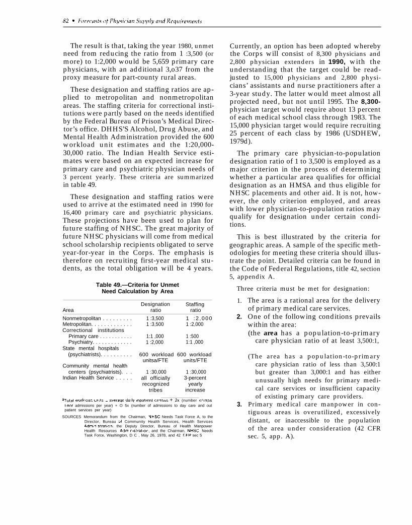
The result is that, taking the year 1980, unmetneed from reducing the ratio from 1 :3,500 (ormore) to 1:2,000 would be 5,659 primary carephysicians, with an additional 3,o37 from theproxy measure for part-county rural areas.
These designation and staffing ratios are ap-plied to metropolitan and nonmetropolitanareas. The staffing criteria for correctional insti-tutions were partly based on the needs identifiedby the Federal Bureau of Prison’s Medical Direc-tor’s office. DHHS’S Alcohol, Drug Abuse, andMental Health Administration provided the 600workload unit estimates and the 1:20,000-30,000 ratio. The Indian Health Service esti-mates were based on an expected increase forprimary care and psychiatric physician needs of3 percent yearly. These criteria are summarizedin table 49.
These designation and staffing ratios wereused to arrive at the estimated need in 1990 for16,400 primary care and psychiatric physicians.These projections have been used to plan forfuture staffing of NHSC. The great majority offuture NHSC physicians will come from medicalschool scholarship recipients obligated to serveyear-for-year in the Corps. The emphasis istherefore on recruiting first-year medical stu-dents, as the total obligation will be 4 years.
Table 49.—Criteria for UnmetNeed Calculation by Area
Designation StaffingArea ratio ratio
Nonmetropolitan . . . . . . . . . 1 :3,500 1 : 2 , 0 0 0Metropolitan. . . . . . . . . . . . . 1 :3,500 1 :2,000Correctional institutions
Primary care . . . . . . . . . . . 1:1 ,000 1 :500Psychiatry. . . . . . . . . . . . . 1 :2,000 1:1 ,000
State mental hospitals(psychiatrists). . . . . . . . . . 600 workload 600 workload
unitsa/FTE units/FTECommunity mental health
centers (psychiatrists). . . 1 :30,000 1 :30,000Indian Health Service . . . . . all officially 3-percent
recognized yearlytribes increase
aTotal workload units ‘= average daily !npatlent census + 2X (number o-f lnPatlent admissions per year) + O 5x (number of admissions to day care and outpatient services per year)
SOURCES Memorandum from the Chairman, NHSC Needs Task Force A, to theDirector, Bureau of Community Health Services, Health ServicesAdmlnlstratlon, the Deputy Director, Bureau of Health ManpowerHealth Resources Admlnlstratlon, and the Chairman, NHSC NeedsTask Force, Washington, D C , May 26, 1978, and 42 CFR sec 5
Currently, an option has been adopted wherebythe Corps will consist of 8,300 physicians and2,800 physician extenders in 1990, with theunderstanding that the target could be read-justed to 15,000 physicians and 2,800 physi-cians’ assistants and nurse practitioners after a3-year study. The latter would meet almost allprojected need, but not until 1995. The 8,300-physician target would require about 13 percentof each medical school class through 1983. The15,000 physician target would require recruiting25 percent of each class by 1986 (USDHEW,1979d).
The primary care physician-to-populationdesignation ratio of 1 to 3,500 is employed as amajor criterion in the process of determiningwhether a particular area qualifies for officialdesignation as an HMSA and thus eligible forNHSC placements and other aid. It is not, how-ever, the only criterion employed, and areaswith lower physician-to-population ratios mayqualify for designation under certain condi-tions.
This is best illustrated by the criteria forgeographic areas. A sample of the specific meth-odologies for meeting these criteria should illus-trate the point. Detailed criteria can be found inthe Code of Federal Regulations, title 42, section5, appendix A.
Three criteria must be met for designation:
1.
2.
3.
The area is a rational area for the deliveryof primary medical care services.One of the following conditions prevailswithin the area:(the area has a population-to-primary
care physician ratio of at least 3,500:1,
(The area has a population-to-primarycare physician ratio of less than 3,500:1but greater than 3,000:1 and has eitherunusually high needs for primary medi-cal care services or insufficient capacityof existing primary care providers.
Primary medical care manpower in con-tiguous areas is overutilized, excessivelydistant, or inaccessible to the populationof the area under consideration (42 CFRsec. 5, app. A).
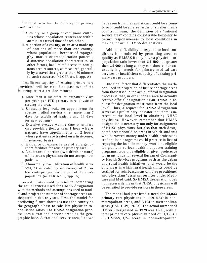
Ch. 3–Requirements ● 8 3
“Rational area for the delivery of primarycare” includes:
i. A county, or a group of contiguous coun-ties whose population centers are within30 minutes travel time of each other.
ii. A portion of a county, or an area made upof portions of more than one county,whose population, because of topogra-phy, market or transportation patterns,distinctive population characteristics, orother factors, has limited access to contig-uous area resources, as measured general-ly by a travel time greater than 30 minutesto such resources (42 CFR sec. 5, app. A).
“Insufficient capacity of existing primary careproviders” will be met if at least two of thefollowing criteria are documented:
a. More than 8,000 office or outpatient visitsper year per FTE primary care physicianserving the area.
b. Unusually long waits for appointments forroutine medical services (i. e., more than 7days for established patients and 14 daysfor new patients).
c. Excessive average waiting time at primarycare providers (longer than 1 hour wherepatients have appointments or 2 hourswhere patients are treated on a first-come,first-served basis).
d. Evidence of excessive use of emergency
e.
f.
room facilities for routine primary care.A substantial portion (two-thirds or more)of the area’s physicians do not accept newpatients.Abnormally low utilization of health serv-ices, as indicated by an average of 2.0 orless visits per year on the part of the area’spopulation (42 CFR sec. 5, app. A).
Several points should be noted in comparingthe actual criteria used for HMSA designationwith the methods and assumptions used to mod-el and project the number of shortage areas an-ticipated in future years. First, the model forpredicting future shortages uses the county asthe geographic base to calculate physician-to-population ratios. The HMSA designation proc-ess uses a “rational service area” as the geo-graphic base. A “rational service area, ” as we
have seen from the regulations, could be a coun-ty or it could be an area larger or smaller than acounty. In sum, the definition of a “rationalservice area” contains considerable flexibility topermit responsiveness to local conditions inmaking the actual HMSA designations.
Additional flexibility to respond to local con-ditions is introduced by permitting areas toqualify as HMSAS if they have a physician-to-population ratio lower than 1:3, 500 but greaterthan 1:3,000 as long as they can show either un-usually high needs for primary medical careservices or insufficient capacity of existing pri-mary care providers.
One final factor that differentiates the meth-ods used in projection of future shortage areasfrom those used in the actual official designationprocess is that, in order for an area to actuallyreceive official designation as an HMSA, a re-quest for designation must come from the locallevel. Thus, a request for HMSA designationserves as a preliminary indicator that there is in-terest at the local level in obtaining NHSCphysicians, However, remember that HMSAdesignation is necessary not only for assignmentof NHSC physicians, but also that such desig-nated areas: would be areas in which studentswho borrowed money under health professionsstudent loan programs could practice in lieu ofrepaying the loans in money; would be eligiblefor grants in various health manpower trainingprograms; would be eligible or given preferencefor grant funds for several Bureau of Communi-ty Health Services programs such as the urbanand rural health initiatives; and would be theonly areas in which rural health clinics could becertified for reimbursement of nurse practitionerand physicians’ assistant services under Medi-care and Medicaid. So HMSA designation doesnot necessarily mean that NHSC physicians willbe recruited to provide services in these areas.
The model had predicted a need for 14,033primary care physicians in 1979, 8,839 in non-metropolitan areas, and 5,194 in metropolitanareas (USDHEW, 1978a). The actual number ofHMSAS designated in 1979 was 1,711, with atotaI primary care physician need of 11,336. Ofthe HMSAS, 1,226 were in nonmetropolitan
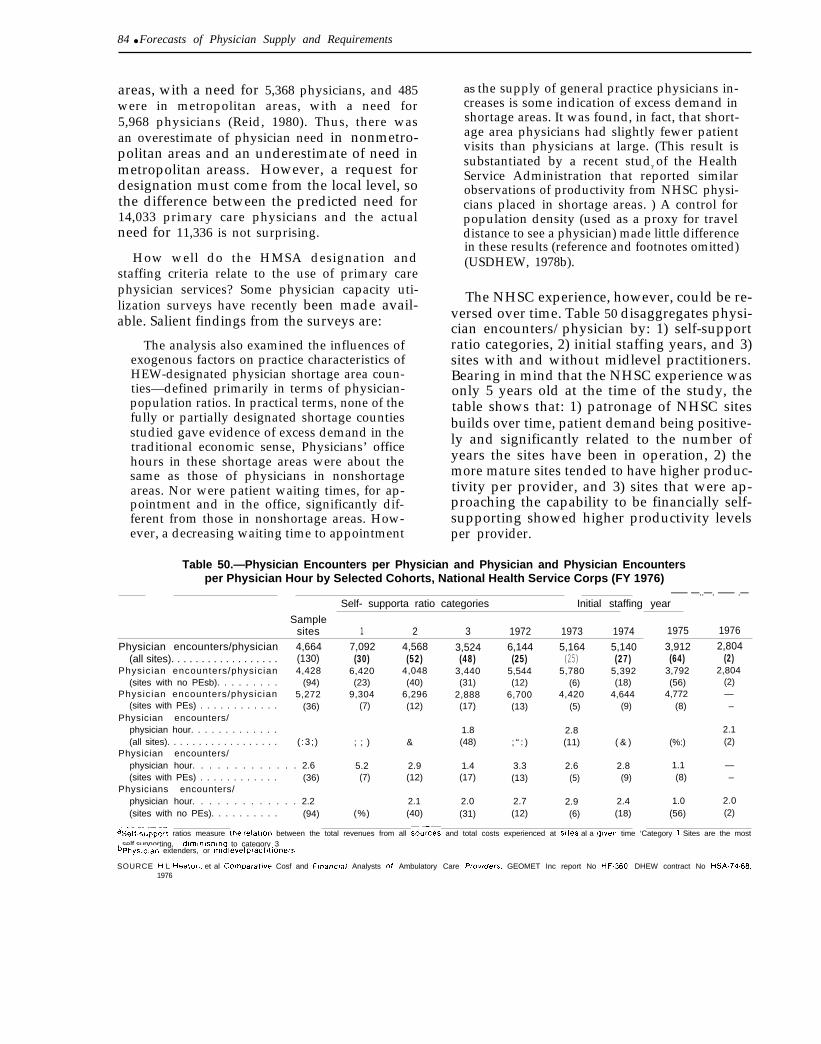
84 ● Forecasts of Physician Supply and Requirements
areas, with a need for 5,368 physicians, and 485were in metropolitan areas, with a need for5,968 physicians (Reid, 1980). Thus, there wasan overestimate of physician need in nonmetro-politan areas and an underestimate of need inmetropolitan areass. However, a request fordesignation must come from the local level, sothe difference between the predicted need for14,033 primary care physicians and the actualneed for 11,336 is not surprising.
How well do the HMSA designation andstaffing criteria relate to the use of primary carephysician services? Some physician capacity uti-lization surveys have recently been made avail-able. Salient findings from the surveys are:
The analysis also examined the influences ofexogenous factors on practice characteristics ofHEW-designated physician shortage area coun-ties—defined primarily in terms of physician-population ratios. In practical terms, none of thefully or partially designated shortage countiesstudied gave evidence of excess demand in thetraditional economic sense, Physicians’ officehours in these shortage areas were about thesame as those of physicians in nonshortageareas. Nor were patient waiting times, for ap-pointment and in the office, significantly dif-ferent from those in nonshortage areas. How-ever, a decreasing waiting time to appointment
as the supply of general practice physicians in-creases is some indication of excess demand inshortage areas. It was found, in fact, that short-age area physicians had slightly fewer patientvisits than physicians at large. (This result issubstantiated by a recent study of the HealthService Administration that reported similarobservations of productivity from NHSC physi-cians placed in shortage areas. ) A control forpopulation density (used as a proxy for traveldistance to see a physician) made little differencein these results (reference and footnotes omitted)(USDHEW, 1978b).
The NHSC experience, however, could be re-versed over time. Table 50 disaggregates physi-cian encounters/physician by: 1) self-supportratio categories, 2) initial staffing years, and 3)sites with and without midlevel practitioners.Bearing in mind that the NHSC experience wasonly 5 years old at the time of the study, thetable shows that: 1) patronage of NHSC sitesbuilds over time, patient demand being positive-ly and significantly related to the number ofyears the sites have been in operation, 2) themore mature sites tended to have higher produc-tivity per provider, and 3) sites that were ap-proaching the capability to be financially self-supporting showed higher productivity levelsper provider.
Table 50.—Physician Encounters per Physician and Physician and Physician Encountersper Physician Hour by Selected Cohorts, National Health Service Corps (FY 1976)
Self- supporta ratio categories—— —..—. —— .—
Initial staffing year
Samplesites 1 2 3 1972 1973 1974 1975 1976
Physician encounters/physician 4,664 7,092 4,568 3,524 6,144 5,164 5,140 3,912 2,804(all sites). . . . . . . . . . . . . . . . . . (130) (30) (52) (48) (25) (25) (27) (64) (2)
Physic ian encounters/physic ian 4,428 6,420 4,048 3,440 5,544 5,780 5,392 3,792 2,804(sites with no PEsb). . . . . . . . . (94) (23) (40) (31) (12) (6) (18) (56) (2)
Physic ian encounters/physic ian 5,272 9,304 6,296 2,888 6,700 4,420 4,644 4,772 —(sites with PEs) . . . . . . . . . . . . (36) (7) (12) (17) (13) (5) (9) (8) –
Physician encounters/physician hour. . . . . . . . . . . . . 1.8 2.8 2.1(all sites). . . . . . . . . . . . . . . . . . ( :3 ; ) ; ; ) & (48) ; “ : ) (11) ( & ) (%:) (2)
Physician encounters/physician hour. . . . . . . . . . . . . 2.6 5.2 2.9 1.4 3.3 2.6 2.8 1.1 —(sites with PEs) . . . . . . . . . . . . (36) (7) (12) (17) (13) (5) (9) (8) –
Physicians encounters/physician hour. . . . . . . . . . . . . 2.2 2.1 2.0 2.7 2.9 2.4 1.0 2.0(sites with no PEs). . . . . . . . . . (94) (%) (40) (31) (12) (6) (18) (56) (2)
ase~f.support ratios measure thi relation between the total revenues from all so;-;ces and total costs experienced at sites al a (Jlven time ‘Category 1 Sites are the mostself.supporting, dlmlnlshlng to category 3
bphyslclan extenders, or mldlevel PraCtltlOnerS
SOURCE f-l L Heaton, et al Comparaf/ve Cosf and Flnanc/af Analysts of Ambulatory Care Provders, GEOMET Inc report No HF360, DHEW contract No HSA.74.68,1976
Bibliography
Aiken, L. H. et al., 1979, “The Contribution ofSpecialists to the Delivery of Primary Care,”New England Journal of Medicine 300:1363-1370.
American Medical Association, 1978, MedicalEducation in the United States, 1977-1978,The Journal of the American Medical Asso-ciation 240: (entire issue).
American Medical News, 1979, p. 10, Dec. 21,1979.
Bureau of Labor Statistics, U.S. Department ofLabor, 1979, Occupational Projections andTraining Data, Washington, D. C.: Govern-ment Printing Office, Bulletin 2020.
Bureau of Labor Statistics, U.S. Department ofLabor, 1979, staff paper in preparation for1990 projections.
Cole, R., 1980, personal communication fromthe Division of Manpower Analysis, Bureauof Health Manpower, with the Office ofTechnology Assessment.
Cultice, J., 1979, personal communication fromthe Division of Manpower Analysis, Bureauof Health Manpower, with the Office ofTechnology Assessment.
Hansen, W. L., 1970, “An Appraisal of Physi-cian Manpower Projections,” Inquiry7:102-113.
.
Heaton, H. L. et al., 1976, Comparative Costand Financial Analysis of Ambulatory CareProviders, GEOMET, Inc., report No.HF-360, DHEW contract No. HSA 674-68.
Hindle, A. et al., 1978, “Estimating the Need forAdditional Primary Care Physicians,”Health Services Research 13:290-304.
Institute of Medicine, National Academy of Sci-ences, 1978, A Manpower Policy for Pri-mary Health Care, Washington, D. C.: Na-tional Academy of Sciences.
Jacoby, I., 1980, personal communication fromthe Deputy Director, Office of GraduateMedical Education, with the Office of Tech-nology Assessment.
JWK International Incorporated, 1979, Evalua-tion of Project SOAR (Supply, Output, andRequirements), draft report, DHEW con-tract No. HRA 232-78-0140.
Kleinman, J. C. and R. W. Wilson, 1977, “Are‘Medically Underserved Areas’ MedicallyUnderserved?” Health Services Research12:147-162.
Lave, J. R. et al., 1975, “Medical ManpowerModels: Need, Demand, and Supply,” in-quiry 12:97-125.
Lee, R. C., 1979, “Designation of Health Man-power Shortage Areas for Use by PublicHealth Service Programs, ” Public Health Re-ports 94:48-59.
McNutt, D., 1979, comments from the Director,Office of Graduate Medical Education, atthe Advisory Panel meeting for this study,Nov. 16,1979, Washington, D.C.
Owens, A., 1977, “How Other Doctors AllocateTheir Time,” Medical Economics, June 13,1977, pp. 105-110.
Owens, A., 1979, “Working at Full Capacity? ALot of Your Colleagues Aren’t,” MedicalEconomics, Apr. 2,1979, pp. 63-71.
Reid, J., 1980, personal communication fromthe Division of Manpower Analysis, Bureauof Health Manpower, with the Office ofTechnology Assessment.
Reinhardt, U., 197s, Physician Productivityand the Demand for Health Manpower, AnEconomic Analysis, Cambridge, Mass.: Bal-linger.
Stambler, H. V., 1979, “Health Manpower forthe Nation—A Look Ahead at the Supplyand the Requirements, ” Public Health Re-ports 94:3-10.
U.S. Department of Health, Education, andWelfare, 1974, The Current and ProjectedSupply of Health Manpower, Summary ofFindings, Washington, D. C.: Bureau ofHealth Resources Development (now the Bu-reau of Health Manpower), Health Re-sources Administration, report No. 75-17.
85
— . . .— .——— . .— .. --—-—. .—.— ——
86 ● Forecasts of Physician Supply and Requirements
1975, impact of National Health hsur-anc;—The Case of the GwnprehensiveHesdth Insurance Plan, An Issue Paper,Washington, D. C.: Bureau of Health Re-sources Development (now the Bureau ofHealth Manpower), Health Resources Ad-ministration.
1977a, Review of Health ManpowerPopulation Requirements Standards, Wash-ington, D. C.: Bureau of Health Manpower,Health Resources Administration, DHEWpublication No. (HRA) 77-22.
1977b, Estimating Manpower Require-ments, A Background Paper Prepared forthe Graduate Medical Education NationalAdvisory Committee, Washington, D. C.:Bureau of Health Manpower, Health Re-sources Administration, report No. 76-114.
1978a, memorandum from the Chair-ma;, NHSC Needs Task Force A, to the Di-rector, Bureau of Community HeaIth Serv-ices, Health Services Administration, theDeputy Director, Bureau of Health Man-power, Health Resources Administration,and the Chairman, NHSC Needs TaskForce, Washington, D. C., May 26,1978.
1978b, Physician Capacity UtilizationSu&eys: Project Summary, Washington,D. C.: Bureau of Health Manpower, HealthResources Administration, DHEW publica-tion No. (HRA) 79-I7.
1978c, Physician Manpower Require-ments, GMENAC Staff Papers #l, Washing-ton, D. C.: Bureau of Health Manpower,Health Resources Administration, DHEWpublication No. (HRA) 78-MI.
19784 Supplg and L7isti”bution of Phy-sici&s and Physician Ektenders, GMENACStaff Papers W, Washi@on, D. C.: Bureauof Health Manpower, Health Resources Ad-ministration, IX+EW publication No. (HRA)78-11.
1978e, Physici4w2 Reqzdremmts Fore-casting: Need-lhsed Vmws Demazd.$asegjMethodologies, GMENAC StSff Paper #3,Washington, D. C.: Bureau of Hkahh Man-power, Health Resources Administration,DHEWpublication No. (I-IRA) 78-12.
1978f, Social and Psychological Char-act&iMics in Medical Specialty mtd Geo-graphic Decisions, GMENAC Staff Paper#4, Washington, D. C.: Bureau of HealthManpower, Health Resources Adminis-tration, DHEW publication No. (HRA)78-13.
-., 1978g, “Federal Support for Health Pro-fessions Education,” options paper, Office ofthe Assistant Secretary for Health, Office ofHealth Policy, Research, and Statistics, July1978.
1979a, Interim Report of the GraduateMe;ical Education National Advisory Com-mittee to the Secretary, Department ofHealth, Education, and Welfare, Washing-ton, D. C.: Health Resources . Admin-istration, DHEW publication No. (HRA)79-633.
1979b, A Report to the President andCo;gress on the Status of Health ProfessionsPersonnel in the United States, Washington,D. C.: Bureau of Health Manpower, HealthResources Administration, DHEW publica-tion No. (HRA) 79-93.
1979c, The Consumer Viewpoint:“Wkat Is Health Care and What Do WeWant?” & A Response, prepared for theGraduate Medical Education National Advi-sory Committee, Washington, D. C.: HealthResources Administration, DHEW publica-tion No. (HRA) 79-632.
1979d, “Outyear Size of the NationalHe&h Service Corps (NHSC)–DECISIONMENKXANDUM,” from the Assistant Sec-retary for Health and the Acting AssistantSecretary for Planning and Evaluation to theSecretary, Washington, D. C., spring 1979.
1979e, Training Health Manpower ForU~ersa-ved Areas, 1973-1979,” A Report tothe People on the National Health ServiceCorps Sc?roZamhip Program, Washington,D. C.: Bureau of Health Manpower, HealthResources Administration, DHEW publica-tion No. (HRA) 79-58.
Walker, J. E. C. and N. L. Armondino, 1977,The Pritnay Care Physician: Issues in Dis-tribution, Lawrence, Kans.: ConnecticutHealth Services Research Series, No. 7.
* Us. al~ P R I N I ’ I N G O F F I C E : 1 9 9 0 0 - 6 0 - 6 1 8