Foreign Direct Investment, Financial Markets and Economic

Growth∗

Laura AlfaroHarvard Business School

Areendam ChandaLouisiana State University

Sebnem Kalemli-OzcanUniversity of Houston and NBER

Selin SayekBilkent University

November 2005(Preliminary)

Abstract

The empirical evidence is such that countries with better developed financial markets gainsignificantly from FDI. This paper formalizes the mechanism through which the trickle downeffect of FDI depends on the extent of the development of the domestic financial sector. Wemodel a small open economy with both foreign and domestic firms producing in the final goodsector. Foreign and domestic firms compete for skilled and unskilled labor and intermediateproducts. Production of intermediate goods is carried out by entrepreneurs in a monopolisticmarket. To run a firm in the intermediate goods sector, entrepreneurs must first engage in R&Din order to develop a new variety of intermediate goods. Innovation, however, requires capitalcosts which must be financed through the domestic financial institutions. If the local financialmarkets are developed enough, they can allow credit constrained entrepreneurs to start theirown firms. This not only spurs entrepreneurial activity but, more importantly, increases thenumber of varieties of intermediate goods which generate positive effects to the final good sectorand allows the economy to benefit from the backward linkages between the foreign and domesticfirms. Our calibration exercise shows that better financial markets allow an economy to takeadvantage of potential linkages from foreign to domestic firms: a 1% increase in FDI generatesfour times more growth for countries with deeper financial markets.

JEL Classification: F23, F36, F43Keywords: Foreign direct investment, financial markets, economic growth, linkages.

∗An earlier version of this paper is circulated under the title “FDI Spillovers, Financial Markets and EconomicDevelopment.” Laura Alfaro, Harvard Business School, 263 Morgan Hall, Boston, MA 02163, lalfaro@hbs.edu.Areendam Chanda, Department of Economics, 2107 CEBA, Louisiana State University, Baton Rouge, LA 70803,achanda@lsu.edu. Sebnem Kalemli-Ozcan, Department of Economics, University of Houston, Houston, Texas, 77204,Sebnem.Kalemli-Ozcan@mail.uh.edu. Selin Sayek, Department of Economics, Bilkent University, Bilkent Ankara06800 Turkey, sayek@bilkent.edu.tr. We are grateful to Pol Antras, Pietro Peretto, Ahmed Mobarak and participantsat the 2005 NEUDC for useful comments and suggestions.

1 Introduction

There is a widespread belief among policymakers and academics that foreign direct investment(FDI) serves as a valuable source of productivity externalities for host countries.1 Prominentmechanisms often highlighted for these externalities are knowledge spillovers and “linkages” be-tween multinationals (MNCs) and domestic firms.2 Local firms can benefit from productivity gains,technology transfers (through formal channels like licensing agreements or through spillovers), em-ployee training, access to markets, among others. Another mechanism for FDI externalities occursthrough backward and forward linkages between foreign and local firms.3 The potential linkageeffects from multinationals firms to domestic firms were highlighted in Albert Hirschman’s (1958)seminal book on this topic. According to Hirschman, one industry may facilitate the developmentof another by easing conditions of production in the other, thereby setting the pace for furtherrapid industrialization. If foreign firms introduce new processes or products to the domestic mar-ket, or buy domestic inputs, for example, domestic firms may benefit.4 Such backward and forwardlinkages between the foreign and domestic firms create an environment where the foreign processescan be easily learned by the domestic firms.

These benefits, together with the direct capital financing it provides, suggest that FDI canplay an important role in modernizing a national economy and promoting economic development.Yet, the empirical evidence has not been able to confirm the existence of such benefits.5 To besure, growth regressions carried out by Borensztein, de Gregorio, and Lee (1998), Carkovic andLevine (2000) and Alfaro, Chanda, Kalemli-Ozcan and Sayek (2004) (ACKS henceforth), find littlesupport that FDI has an exogenous positive effect on economic growth. Hence, there appears tobe a significant gap between the consensus among practitioners and the evidence regarding theimportance of positive FDI externalities.

While it may seem natural to argue that FDI can convey greater knowledge spillovers, a coun-try’s capacity to take advantage of these externalities might be limited by local conditions, such asthe development of the local financial markets or the educational level of the country- two exam-ples of absorptive capacities that have recently received attention in the empirical FDI and growthliterature.6 ACKS, Durham (2004) and Hermes and Lensink (2003) provide evidence that, indeed,

1See Blomstrom and Kokko (1998) for an overview of the different channels.2A multinational corporation (MNC) or enterprise (MNE) is a firm that owns and controls production facilities

or other income-generating assets in at least two countries. When a foreign investor begins a green-field operation(i.e., constructs new production facilities) or acquires control of an existing local firm, that investment is regarded asa direct investment in the balance of payments statistics. An investment tends to be classified as direct if a foreigninvestor holds at least 10% of a local firm’s equity. This arbitrary threshold is meant to reflect the notion that largestockholders, even if they do not hold a majority stake, will have a strong say in a company’s decisions and participatein and influence its management. Hence, to create, acquire or expand a foreign subsidiary, MNE’s undertake FDI. Inthis paper, we often refer to MNEs and FDI interchangeably.

3A “forward linkage” industry is one that lowers the cost of production for another activity. A “backward linkage”raises the demand for another activity.

4For a theoretical treatment of multinationals and linkages see Rodriguez-Clare (1996) and Markusen and Venables(1999); and Alfaro and Rodriguez-Clare (2004) for an empirical analysis.

5The vast literature on foreign direct investment and multinational corporations has been surveyed many times.See Barba Navaretti and Venables (2004) for a recent overview of the main issues and findings.

6Borensztein et al. (1998) and Xu (2000) show that FDI allows for transferring technology and for higher growth

1

countries with well-developed financial markets gain significantly from FDI in terms of their growthrates.

In this paper, our objective is to a) formalize the mechanism through which the trickle downeffect of FDI depends on the extent of the development of the local financial sector, and b) use theformal model to quantitatively gauge how the response of growth to FDI varies with the level ofdevelopment of the financial markets. We model a small open economy with foreign and domesticfirms producing in the competitive final good sector. The production of final goods combinesdomestic unskilled labor and human capital (skilled labor) and domestically produced intermediategoods characterized by a Dixit-Stiglitz-Ethier love of variety production function.7 Production ofintermediate goods is carried out by entrepreneurs in a monopolistic market. In order to be ableto run a firm in the intermediate good sector, entrepreneurs must first engage in R&D in order todevelop a new variety of intermediate goods. Innovation in the intermediate good sector, however,requires capital costs which must be financed by borrowing from the domestic financial institutions,which intermediate funds at a positive cost. If the local financial markets are developed enough,credit constrained entrepreneurs will start their own firms. This not only spurs entrepreneurialactivity but, more importantly, increases the number of varieties of intermediate goods therebygenerating positive effects to the final good sector and, in particular, positive externalities toother domestic firms that use those inputs. In other words, in this model FDI increases thedemand for intermediate goods, and well-developed financial markets ease fulfilling this increaseddemand, thereby allowing for further possible positive effects of FDI to the local economy. LikeHirschman (1958), we view linkages here as pecuniary externalities. In contrast to knowledgespillovers, pecuniary externalities take place through market transactions. In our model, linkagesare associated with pecuniary externalities in the production of inputs. The existence of suchpecuniary externalities where both national firms and foreign firms use intermediate products froma local industry has been noted by Barba Navaretti and Venables (2004, p.41). Hobday (1995),in a case study of developing East Asia, finds many situations in which MNCs investment createdbackward linkages effects to local suppliers. Javorcik (2004) presents additional evidence on verticalspillovers to downstream suppliers to MNCS.

The importance of well-functioning financial institutions in augmenting technological innova-tion, capital accumulation, and economic development has been recognized and extensively dis-cussed in the literature.8 Furthermore, as McKinnon (1973) stated, the development of capital

only when the host country has a minimum threshold stock of human capital, and that most LDCs do not meet thisthreshold.

7One question is why under such circumstances entrepreneurs would benefit from starting a new firm in thepresence of FDI. This can be for two reasons. Entrepreneurs (suppliers), due to high setup costs and costs ofexporting, may not start a business unless they have a big enough domestic demand. Foreign firms may generate theneeded higher domestic demand. In addition, domestic suppliers may benefit through technology transfers. Thereis evidence that multinational companies tend to share their knowledge and technological advances with local firms,in particular downstream suppliers. Additional benefits can accrue via knowledge externalities. An earlier version ofthe paper considered knowledge spillovers.

8Goldsmith (1969), McKinnon (1973), Shaw (1973), followed by Boyd and Prescott (1986), Greenwood and Jo-vanovic (1990), and King and Levine (1993b), among others, have shown that well-functioning financial markets, bylowering the costs of conducting transactions, ensure capital is allocated to the projects that yield the highest returns,

2

markets is “necessary and sufficient” to foster the “adoption of best-practice technologies andlearning by doing.” In other words, limited access to credit markets restricts entrepreneurial de-velopment. In this paper, we extend this view and argue that the lack of development of localfinancial markets can limit the economy’s ability to take advantage of potential FDI spillovers.If entrepreneurship allows greater assimilation and adoption of best technological practices madeavailable by FDI, then the absence of well-developed financial markets limits the potential posi-tive FDI externalities. In addition, as our model shows, the absence of well-developed financialmarkets may impede entrepreneurs and the economy as a whole from benefitting from potentialbackward linkages to foreign firms.9 An excellent example is the involvement of Suzuki in India.Suzuki entered into a joint venture with the Government of India in 1981 to manufacture small-sized affordable cars. Initially, all the car’s parts were imported from Japan. Within ten years,the plant had become the center of gravity of scores of ancillary parts manufacturers that did notexist earlier. Today, these suppliers provide ninety percent of a car’s parts.10 Without externalfinancing, it is unlikely that these manufacturers would have emerged. In similar vein, followingIntel’s construction of a semiconductor assembly plant in Costa Rica in 1996, local software pro-duction in Costa Rica increased dramatically. Evidence indicates that the sector benefited fromnewly created training programs in higher education institutions that became “Intel Associates.”However, producers and potential entrepreneurs in the software sector continuously complain thata lack of funds and/or the high cost of available financing hinder the growth of the sector and itsability to compete in the international arena.11

The main result is confirmed in the numerical exercises we conduct. Our numerical exercisesshow that better financial markets allow an economy to take advantage of potential linkages fromforeign to domestic firms: a 1% increase in FDI generates four times more growth for the countrieswith deeper financial markets.

Overall, the model closely follows Grossman and Helpman’s (1990, 1991) small open economysetup of endogenous technological progress resulting from the innovation in the intermediate goodssector. This basic framework is modified to incorporate foreign firms and financial intermediation.12

This standard setting is preferred since it provides the most transparent solution and interpretationof our hypothesis.13 The model shares with King and Levine (1993) the Schumpeterian view that

and therefore enhance growth rates.9The old development literature had already raised concerns about the negative effects of MNC to the domestic

economy. Critics argued that MNCs favored imported inputs over locally produced ones, with negative consequenceson local production. Hirschman (1958) warned that in the absence of linkages, foreign investments could have limitedor even negative effect in an economy (the so called “enclave economies”).

10See Parikh (1997) p.138.11On Intel in Costa Rica, see Spar (1998), Hanson (2001), Larrain, Lopez-Calva and Rodriguez-Clare (2000). On

the financing issues, see Perez (2000).12See Rodriguez-Clare (1996) for similar treatment of MNCs.13Similarly, Gao (2005) incorporates FDI into a growth model that closely follows Grossman and Helpman (1991).

The author, however, does not model the role of domestic financial markets in allowing FDI benefits to materialize.Other models that have incorporated financial intermediaries in the endogenous growth framework include King andLevine (1993), who develop a model that incorporates financial markets in endogenous growth models. This paperbrings together both foreign firms and financial markets into the basic endogenous growth framework.

3

financial institutions are crucial for fostering entrepreneurial activity.14 Furthermore, the paperrelates to the much broader literature that studies the role played by financial markets in allowingthe benefits of the interaction with the international markets, or in other words globalization, tomaterialize.15

The rest of the paper is organized as follows. Section 1 presents the benchmark model. Section2 solves for the analytical case. Section 3 simulates the model for plausible parameter values. Thelast section concludes.

2 Basic Model

Consider a small open economy. The economy is populated by a continuum of infinitely livedagents of total mass 1. Agents derive utility from the consumption of final goods. There are twohomogeneous final goods in the economy, Yd and Yf , produced by the domestic and the foreignsector, respectively. The final good is freely traded in the world markets, and the domestic economyis small in the sense that is does not affect the international price denoted by P .

Final goods production combines domestic unskilled labor and skilled labor (human capital)together with a composite intermediate good I, which is assembled from a continuum of horizontallydifferentiated goods (continuum of varieties x). Labor, unskilled and skilled (human capital), arenot traded and available in a fixed quantity L and H, correspondingly. Competition in the labormarket ensures that unskilled and skilled wages, wu and ws, are equal to their respective marginalproducts. To capture the importance of proximity between suppliers and users of inputs, weassume that all varieties of intermediate goods are non-traded. Local production of a wide varietyof specialized inputs improves the efficiency of local firms producing final goods. Intermediategoods, which are produced in a monopolistic market, are produced by entrepreneurs who alsoengage in research and development (R&D). In order to run a firm in the intermediate good sector,entrepreneurs must first develop a new variety of intermediate goods. Since this is a small openeconomy, R&D activities do not affect conditions abroad. Innovation occurs only in the intermediate(non-traded) good sector. Innovation in the intermediate good sector, however, requires capitalcosts which must be financed by borrowing from the domestic financial institutions. In otherwords, entrepreneurs must finance R&D costs in the the local financial markets, and they willengage in R&D and production of intermediate goods only if the present value of the stream ofmonopolistic profits of operating a firm in the intermediate good sector are greater than the capitalcosts of innovating.

Finally, the domestic financial system intermediates funds domestically at an additional cost.This cost reflects the level of development of the domestic financial markets; lower levels of devel-

14See also see Aghion, Howitt and Mayer-Foulkes (2005) for a theoretical and empirical application of imperfectfinancial markets in Schumpeterian growth models.

15Aghion, Bacchetta, Ranciere and Rogoff (2005) find that a country’s choice of exchange rate regime can havea significant impact on its long-term rate of productivity growth. The authors find this impact to depend on thecountry’s level of financial development. Chang, Kaltani and Loayza (2005) show the effects of trade openness oneconomic growth depend, among other structural characteristics, on the financial development of a country. Thesequencing literature has argued that well developed financial markets are crucial for successful reforms.

4

opment of the local financial markets are associated with higher costs. This manifests itself in ahigher borrowing rate, i which is greater than the lending rate, r. In the main text of the paperwe do not model the source of this cost. However in the appendix we propose a simple version ofthe cost verification approach that has the same implications.

2.1 Households

Households maximize utility over the consumption of final goods,

U =∫ ∞

0e−ρt log u(Ct)dt (1)

where u(.) is a continuously differentiable strictly concave utility function, ρ is the time pref-erence parameter, and Ct denotes consumption of the final good at time t. Notice that for theconsumer, final goods produced either by local or foreign firms, are homogeneous.

Consumers maximize utility subject to the intertemporal budget constraint.

∫ ∞

0e−rtPtCtdt ≤

∫ ∞

0e−rtwtdt + A0 (2)

where A0 denotes the value of the assets held by the household at t = 0 and wt the wage income,skilled (ws) or unskilled (wu). The intertemporal budget constraint requires that the present valueof all expenditures, Et = PtCt, do not exceed the present value of factor income plus the value ofasset holdings in the initial period. The solution of this standard problem implies that the valueof the expenditure must grow at a rate equal to the difference between the interest rate and thesubjective discount rate.

.E

E= r − ρ (3)

Since the economy has access to the international capital markets, equilibrium conditions requirethat rather than the trade balance, Et = PtCt, being balanced each period, the present value of thetrade balance,

∫∞0 e−rtPtCtdt, be balanced. As seen in equation (2), this condition is automatically

guaranteed by the restriction imposed by the intertemporal budget constraint.16

Note also that the distribution between skilled and unskilled workers is immaterial in the so-lution of the consumer problem because the rate of growth of expenditures would be the same forall agents. The only restriction required is that each household obeys its intertemporal budgetconstraint.

2.2 Production

2.2.1 The Final Goods Sector

The domestic sector, denoted Yd, is entirely owned by domestic producers. These producers combinedomestically supplied skilled (human capital) and unskilled labor and an intermediate good using

16Note that, given the homogeneity of the two goods, our economy is really a one good economy, rendering thediscussion of trade balance arguably immaterial.

5

the following Cobb-Douglas constant returns to scale technology,

Yt,d = At,dLβdt,dH

γdt,dI

1−γd−βdt,d (4)

with 0 < βd < 1, 0 < γd < 1, where Lt,d denotes the unskilled labor used in the domestic productionin period t, Ht,d is the skilled labor used in the domestic production in period t, It,d is the amountof composite intermediate goods used in the domestic production in period t and At,d representsthe productivity parameter in the domestic sector in period t.

The foreign sector, denoted Yf , is owned by foreign investors and uses domestically suppliedlabor. Foreign firms can be thought of as owning the technology to produce the good Yf andbecause of its special characteristics, they choose to directly produce in the country rather thanto license the technology. The industrial organization literature suggests that firms engage in FDInot because of differences in the cost of capital but because certain assets are worth more underforeign than local control. If lower cost of capital were the only advantage a foreign firm has overdomestic firms, it would still remain unexplained why a foreign investor would endure the troublesand headaches of operating a firm in a different political, legal, and cultural environment instead ofsimply making a portfolio investment. In addition, evidence shows that investors often fail to bringall the capital with them when they take control of a foreign company; instead, they tend to financean important share of their investment in the local market. Moreover, FDI flows, in particular thoseamong developed countries, proceed in both directions and often in the same industry. CharlesKindleberger (1969, p.3) noted, “direct investment may thus be capital movement, but it is morethan that.” An investor’s decision, then, to acquire a foreign company or build a plant instead ofsimply exporting or engaging in other forms of contractual arrangements with foreign firms involvesthree interrelated aspects: ownership of an asset, location to produce, and whether to keep the assetinternal to the firm.17 First, a firm can possess some ownership advantage – a firm-specific assetsuch as a patent, technology, process, or managerial or organizational know-how – that enablesit to outperform local firms.18 Second, locational factors, such as opportunities to tap into localresources, providing access to low-cost inputs or low-wage labor, or bypass tariffs that protecta market from imported goods can also lead to the decision to invest in a country rather thanserve the foreign market through exports. Third, the internalization of global transactions may bepreferable to the use of arm’s-length market transactions.19 Since our objective in this paper is tounderstand the effects of foreign production on local output and the role of financial markets, andnot the decision to investment abroad, we model the frictions of doing business in the domesticeconomy with the function φ.20

Foreign firms use the following Cobb-Douglas constant returns to scale production function,17This approach to the theory of the multinational firm is also known as the OLI framework. See Dunning (1981).18However, this also means that a foreign firm will seek to use this special asset to its advantage and prevent leakages

of its technology. Hence, in the model, potential benefits from FDI occur from linkages (pecuniary externalities) andnot through technology spillovers.

19For models that endogeneize FDI decision see Baraba-Navaretti and Venables (2004).20Burnstein and Monge-Naranjo (2005) assume taxes on foreign firms to be the policy barrier in each country. We

follow a broader interpretation, as foreign firms need to compensate for a wide range of costs/risks of doing businessabroad including institutions, sovereign risk, taxes, infrastructure in the country, etc.

6

Yt,f =1φ

At,fLβf

t,fHγf

t,fI1−γf−βft,f (5)

with 0 < βf < 1, 0 < γf < 1, where, Lt,f denotes the domestic labor in the foreign sector inperiod t, Ht,d is the skilled labor used in the domestic production in period t, It,f is the amount ofcomposite good of intermediate goods used in the foreign production in period t, At,f representsthe productivity parameter in the foreign sector at time t and φ the frictions of doing business ina foreign country.21

Lastly, the final good is assembled from differentiated intermediate inputs or “producer ser-vices.” As mentioned, the intermediate input is not traded. Intermediate goods are produced overa continuum of varieties. Following Ethier (1982), we assume that, for a given aggregate quantityof intermediate inputs used in final production, output is higher the greater the diversity in theset of inputs used.22 This specification captures the productivity gains from increasing degrees ofspecialization in the production of final goods.

It,s =

[∫ n(t)

0xt,s(i)αdi

]1/α

(6)

where s corresponds to either the domestic or foreign sector, varieties are index by i, xt,s(i) isthe amount of each intermediate good i used in the production of the final good by sector s, nt isthe measure of the number of varieties available at t. Let p(i) denote the price of a variety i of theintermediate good x. This CES specification imposes a constant and equal elasticity of substitutionbetween a pair of inputs. It is straightforward to show that the elasticity of substitution betweenany two inputs is given by ε = 1/(1 − α). The specification of the production function impliesthat there are returns from the division of labor in the production of intermediate goods. In asymmetric equilibrium all intermediate goods are priced similarly, pi(xi) = px. Hence, because ofthe symmetric way in which different varieties enter into the production function and convexity,efficiency requires firms producing final goods to use the same quantity of all available varieties,x(i) = x. Let Xt,s =

∫ n(t)0 xt(i)di = ntxt be the aggregate quantity of intermediate goods

employed in the production of the final good by sector s (domestic or foreign) at time t, then

we can rewrite It,s =[∫ n(t)

0 xt(i)αdi]1/α

= xtn1/αt as It,s = n

1−αα

t Xt,s. With 0 < α < 1, theproductivity of a given stock of resources rises with the number of varieties (ε > 1).

We can then rewrite the production function for each sector s as:

Yt,d = At,dLβdt,dH

γdt,dX

1−γd−βdt,d n

(1−γd−βd)(1−α)

αt (7)

21Note that Grossman and Helpman (1990, p.147) assume that all sectors are equally intensive in their use ofintermediate products in order to ensure the existence of a balance growth path. As they note, without this assumptionthe importance of one sector would decline over time until that sector eventually vanishes in the long run equilibrium.Our model has 3 factors which allows for greater flexibility. However, for analytical tractability, we later imposerestrictions on the parameter values to obtain a balanced growth path and a closed form solution.

22The intermediate goods sector uses the functional form introduced by Dixit and Stiglitz (1978) proposed as aspecification for a utility function and later applied to production theory by Ethier (1982).

7

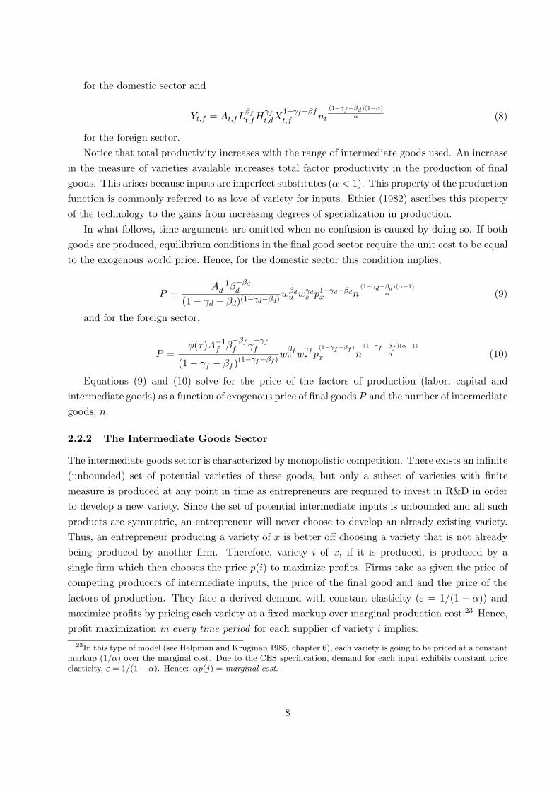
for the domestic sector and

Yt,f = At,fLβf

t,fHγf

t,dX1−γf−βft,f nt

(1−γf−βd)(1−α)

α (8)

for the foreign sector.Notice that total productivity increases with the range of intermediate goods used. An increase

in the measure of varieties available increases total factor productivity in the production of finalgoods. This arises because inputs are imperfect substitutes (α < 1). This property of the productionfunction is commonly referred to as love of variety for inputs. Ethier (1982) ascribes this propertyof the technology to the gains from increasing degrees of specialization in production.

In what follows, time arguments are omitted when no confusion is caused by doing so. If bothgoods are produced, equilibrium conditions in the final good sector require the unit cost to be equalto the exogenous world price. Hence, for the domestic sector this condition implies,

P =A−1

d β−βdd

(1− γd − βd)(1−γd−βd)wβd

u wγds p1−γd−βd

x n(1−γd−βd)(α−1)

α (9)

and for the foreign sector,

P =φ(τ)A−1

f β−βf

f γ−γf

f

(1− γf − βf )(1−γf−βf )w

βfu w

γfs p

(1−γf−βf )

x n(1−γf−βf )(α−1)

α (10)

Equations (9) and (10) solve for the price of the factors of production (labor, capital andintermediate goods) as a function of exogenous price of final goods P and the number of intermediategoods, n.

2.2.2 The Intermediate Goods Sector

The intermediate goods sector is characterized by monopolistic competition. There exists an infinite(unbounded) set of potential varieties of these goods, but only a subset of varieties with finitemeasure is produced at any point in time as entrepreneurs are required to invest in R&D in orderto develop a new variety. Since the set of potential intermediate inputs is unbounded and all suchproducts are symmetric, an entrepreneur will never choose to develop an already existing variety.Thus, an entrepreneur producing a variety of x is better off choosing a variety that is not alreadybeing produced by another firm. Therefore, variety i of x, if it is produced, is produced by asingle firm which then chooses the price p(i) to maximize profits. Firms take as given the price ofcompeting producers of intermediate inputs, the price of the final good and and the price of thefactors of production. They face a derived demand with constant elasticity (ε = 1/(1 − α)) andmaximize profits by pricing each variety at a fixed markup over marginal production cost.23 Hence,profit maximization in every time period for each supplier of variety i implies:

23In this type of model (see Helpman and Krugman 1985, chapter 6), each variety is going to be priced at a constantmarkup (1/α) over the marginal cost. Due to the CES specification, demand for each input exhibits constant priceelasticity, ε = 1/(1− α). Hence: αp(j) = marginal cost.

8

max πi = pixi − ci(wu, ws, xi)xi (11)

where ci(wu, ws, xi) represents the marginal cost to be defined in what follows and xi = xd +xf ,is the sum of the demand of intermediate product i by domestic and foreign firms respectively.

Production of intermediate goods require both skilled and unskilled labor according to thefollowing specification:

x = LδxH1−δ

x (12)

Hence, the cost function for the intermediary monopolist is given by:

cx (wu, ws, xi) = δ−δ(1− δ)−(1−δ)wδuw(1−δ)

s x (13)

As is well known in these models, the profit maximization solution yields a markup price ofp(i) = ci(.)/α. Hence, the price of the intermediate goods is given by,

px = δ−δ(1− δ)−(1−δ) wδuw

(1−δ)s

α(14)

Before we proceed, note that from the Cobb Douglas production function, the fraction thatdomestic firms spends on all intermediate goods is given the corresponding share in the productionfunction, (1− γd − βd) pY Yd. This implies that for each intermediate good, the amount spent bydomestic firms is given by,

(1− γd − βd) PYd

n(15)

by similar logic, the amount that foreign firms spend on these goods is given by

(1− γf − βf ) PYf

n(16)

The sum of (15) and (16) must be the revenue of each intermediate producer:

pixi =(1− γd − βd) PYd

n+

(1− γf − βf ) PYf

n(17)

Therefore another way to write the operating profits per firm is:

πi =(1− α) P

n[(1− γd − βd) Yd + (1− γd − βf ) Yf ] (18)

The Value of the Monopolistic Firm Let v(t) denote the value of a claim to the infinitestream of profits to a typical firm at time t. The present discounted value of an infinite stream ofprofits for a firm that supplies intermediate goods is given by,

v(t) =∫ ∞

te−r(τ−t)π(τ)dτ

9

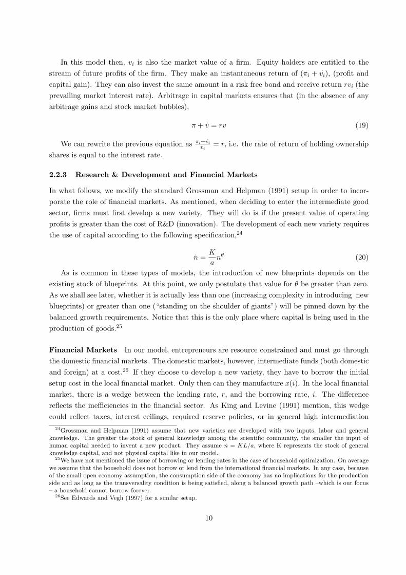
In this model then, vi is also the market value of a firm. Equity holders are entitled to thestream of future profits of the firm. They make an instantaneous return of (πi +

.vi), (profit and

capital gain). They can also invest the same amount in a risk free bond and receive return rvi (theprevailing market interest rate). Arbitrage in capital markets ensures that (in the absence of anyarbitrage gains and stock market bubbles),

π + v = rv (19)

We can rewrite the previous equation as πi+.vi

vi= r, i.e. the rate of return of holding ownership

shares is equal to the interest rate.

2.2.3 Research & Development and Financial Markets

In what follows, we modify the standard Grossman and Helpman (1991) setup in order to incor-porate the role of financial markets. As mentioned, when deciding to enter the intermediate goodsector, firms must first develop a new variety. They will do is if the present value of operatingprofits is greater than the cost of R&D (innovation). The development of each new variety requiresthe use of capital according to the following specification,24

n =K

anθ (20)

As is common in these types of models, the introduction of new blueprints depends on theexisting stock of blueprints. At this point, we only postulate that value for θ be greater than zero.As we shall see later, whether it is actually less than one (increasing complexity in introducing newblueprints) or greater than one (“standing on the shoulder of giants”) will be pinned down by thebalanced growth requirements. Notice that this is the only place where capital is being used in theproduction of goods.25

Financial Markets In our model, entrepreneurs are resource constrained and must go throughthe domestic financial markets. The domestic markets, however, intermediate funds (both domesticand foreign) at a cost.26 If they choose to develop a new variety, they have to borrow the initialsetup cost in the local financial market. Only then can they manufacture x(i). In the local financialmarket, there is a wedge between the lending rate, r, and the borrowing rate, i. The differencereflects the inefficiencies in the financial sector. As King and Levine (1991) mention, this wedgecould reflect taxes, interest ceilings, required reserve policies, or in general high intermediation

24Grossman and Helpman (1991) assume that new varieties are developed with two inputs, labor and generalknowledge. The greater the stock of general knowledge among the scientific community, the smaller the input ofhuman capital needed to invent a new product. They assume

.n = KL/a, where K represents the stock of general

knowledge capital, and not physical capital like in our model.25We have not mentioned the issue of borrowing or lending rates in the case of household optimization. On average

we assume that the household does not borrow or lend from the international financial markets. In any case, becauseof the small open economy assumption, the consumption side of the economy has no implications for the productionside and as long as the transversality condition is being satisfied, along a balanced growth path –which is our focus– a household cannot borrow forever.

26See Edwards and Vegh (1997) for a similar setup.

10

costs due to labor regulation, high administration costs, low technology, etc.27 This simplificationallows us to focus on the main theme of the paper: the role of financial markets in allowing FDIbenefits to materialize. Thus, this assumption should be regarded as a shortcut to more complexmodelling of the financial sector.28 The reader is referred to the appendix for a cost verificationapproach that yields the similar implications.

Therefore the cost of one blueprint isia

nθ(21)

For example, given nθ and a, if an entrepreneur wants to introduce one blueprint at any instantin time, the amount of capital needed will be K = a/nθ, so that n = 1 and hence its payments willbe ia

nθ .29

There is free entry in to the R&D sector. Entrepreneurs will have an incentive to develop newblueprints if ia

nθ < v. Note, however, that this conditions implies that the demand for capital willbe infinite, which cannot be a general equilibrium solution. Hence, we can rule out this conditionex ante. If on the other hand ia

nθ > v, entrepreneurs will have no incentives to create new blueprintsand hence there will be no new investment in R&D. This possibility cannot be ruled out ex ante.Therefore, in equilibrium, entrepreneurs will not earn excess returns as long as

ia

nθ≥ v

andia

nθ= v whenever n > 0 (22)

in other words, the condition with hold with equality whenever there is growth.30

Before we proceed, notice that if v is the value of one firm, then the aggregate value is nv. Letthe inverse of nv be equal to V ,

V = 1/nv (23)

We can rewrite the no arbitrage equation (19), as πv + v

v = r. Note that vv = −θ n

n from equation(22), i.e. more blueprints reduce the value of each firm. Using the latter expression and arbitragecondition in the capital markets, (23), we can rewrite (19) as,

V nπ − θn

n= r (24)

27Galor and Zeira (1993) adopt a similar strategy to allow for capital market imperfections.28There is a broad literature modelling how information and transaction costs can explain the emergence of fi-

nancial intermediaries. Financial institutions can economize on trading costs (Townsend, 1978); pool liquidity risk(Diamond and Dybig, 1983); acquire information on investment projects (Boyd and Prescott, 1986); and reduce thecost of monitoring entrepreneurs (Diamond, 1984). Other researches, such as Greenwood and Jovanovic (1980), Ben-civenga and Smith (1991), King and Levine (1993), Acemoglu and Zilibotti (1997, 1999), have built growth modelsincorporating the role of financial markets. See Levine (1997) for a review the literature.

29Since the evidence seems to indicate the development of the overall domestic financial market, which includes,for example, the stock market in addition to the banking system, more generally, we can think that the cost of oneblue print as Ψa

nθ , were Ψ represents the higher cost of intermediation faced in the domestic market.30To rule out arbitrage gains, it must be that,

∫∞t

e−r(τ−t)π(τ)dτ = (r+δ)a

nθ ⇒ ∫∞t

e−r(τ−t)(1− α)pixidτ = (r+δ)a

nθ .

Differentiating this equation with respect to t we find: r = (1−α)pixi(r+δ)a

− θ nn.

11

Using the per firm profit equation (18) and (23), we obtain,

(1− α) P

ia

[(1− γd − βd)

Yd

n1−θ+ (1− γf − βf )

Yf

n1−θ

]− θ

n

n= r (25)

Notice that in the previous equation, higher foreign firm production, Yf increases the growthrate of n

n . On the other hand, notice that if intermediation costs increase(i goes up), the growthrate would be lower. In order to further simplify the previous relation, consider Yd

n1−θ = Yd andYf

n1−θ = Yf as efficiency units of output in the two sectors.

(1− α) P

ia

[(1− γd − βd) Yd + (1− γf − βf ) Yf

]− θ

n

n= r (26)

Note that by similar logic we can rewrite equation (20) as

n

n=

1a

K

n1−θ=

1aK

where K is the capital stock per efficiency unit.

2.3 Solving the Model

2.3.1 Defining the Balanced Growth Path

Substituting the price for intermediate inputs (14) into the equilibrium conditions of the domes-

tic sector (9) and foreign sector (10), and defining wi,d = wi,d/(n

1−αα

1(1−γd−βd)

)and wi,f =

wi,f/

(n

1−αα

1(1−γf−βf )

)for the domestic and foreign sector, respectively, we obtain the following

expressions for the domestic and foreign sectors equilibrium conditions,

P =A−1

d β−βdd γ−γd

d

(1− γd − βd)(1−γd−βd)

(δ−δ(1− δ)−(1−δ)

α

)1−γd−βd

(wu,d)βd+δ(1−γd−βd) (ws,d)

γd+(1−δ)(1−γd−βd)

(27)

P =φ(τ)A−1

f β−βf

f γ−γf

f

(1− γf − βf )(1−γf−βf )

(δ−δ(1− δ)−(1−δ)

α

)(1−γf−βf )

wβf+δ(1−γf−βf)u w

γf+(1−δ)(1−γf−βf)s (28)

Notice that since P and the other parameters in the previous equations are all constant, in orderto obtain balanced growth path, the rate of growth of wu, ws and px, must all be linear functionsof the growth rate of n. For example, the rate of growth of w

βd+δ(1−γd−βd)u w

γd+(1−δ)(1−γd−βd)s has

to be equal to the rate of growth of n(1−γd−βd)(1−α)

α . Similarly, the rate of growth of

wβf+δ(1−γf−βf)u w

γf+(1−δ)(1−γf−βf)s has to be equal to the rate of growth of n

(1−γf−βf )(α−1)

α .

Therefore:

(βd + δ (1− γd − βd))wu

wu+ (γd + (1− δ) (1− γd − βd))

ws

ws=

(1− γd − βd)(1− α)α

n

n(29)

12

(βf + δ (1− γf − βf ))wu

wu+ (γf + (1− δ) (1− γf − βf ))

ws

ws=

(1− γf − βf )(1− α)α

n

n(30)

Note that a sufficient condition to obtain a balanced growth path for factor prices is then(1− γf − βf ) = (1− γd − βd) = λ. In what follows, we make this assumption in order to derive ananalytical solution:

Assumption 1 (1− γf − βf ) = (1− γd − βd) = λ

Corollary 2 γf − γd = βd − βf .

2.3.2 Labor Market Conditions

Equilibrium conditions in the labor market imply that the labor employed by the domestic, theforeign and the intermediate good sectors add up to the total supply in the economy. This implies,for the skilled and unskilled labor, respectively,

Ld + Lf + nLx = L (31)

Hd + Hf + nHx = H (32)

The equilibrium factor prices can in fact be derived directly from equations (27) and (28),31

wu = P

(δδ(1− δ)(1−δ)

α

)λ 1(

Adββdd γγd

d λλ)

γf +(1−δ)λ

γd−γf

Afβ

βf

f γγf

f λλ

φ

(γd+(1−δ)λ)γd−γf

(33)

ws = P

(δδ(1− δ)(1−δ)

α

)λ (Adβ

βdd γγd

d λλ)(βf +δλ)

γd−γf

φ

Afββf

f γγf

f λλ

βd+δλ

γd−γf

(34)

The model follows standard comparative statics of a two sector general equilibrium model. Considerthe case where multinationals use skills more intensively, that is γf > γd.32 Given fixed resourceendowments, an improvement in Af , the technology of the skill intensive sector, raises the demandfor skills more than it raises the demand for raw labor. As a result this creates an upward pressureon skilled labor wages. It also raises the share of the foreign firms in total output. This creates an

31We have also used the fact that if γd−γf = βf −βd, then (βf + δλ) (γd + (1− δ) λ)−(βd + δλ) (γf + (1− δ) λ) =γd − γf (= βf − βd) .

32As Barba Navaretti and Venables (2004) note, there is ample evidence that foreign firms employ more skilledpersonnel than domestic firms. They also tend to be larger, more efficient, and pay higher wages. This could be bothbecause MNCs bring to host countries a knowledge that may not necessarily be available in the domestic economy(technologies, management skills, market access and others) or because foreign firms cherry pick the best firm orsectors. When adopting stringent econometric techniques, the differences between foreign and domestic firms aresmall and not always significant. But foreign firms are still found to perform better in some cases and never worsethan local firms. Foreign firms are also found to pay higher wages than local firms, even after controlling for skilldifferences and for firm-specific factors.

13

excess supply of unskilled labor since domestic firms use this kind of labor relatively intensively.As a result skilled labor wages rise and unskilled labor wages fall. Of course the opposite happensif Ad increases. Finally all of this hinges on the assumption that the multinationals use skilledlabor more intensively. If the opposite were true, then increased entry of multinationals would havethe reverse effect. Finally, these wage rates themselves are not functions of the domestic resourceendowment. The exogenous price of the final good along with other production parameters pindown the wage rates.

2.3.3 Output and Capital

Solving for Output Using the cost functions for the domestic, foreign and intermediate goodssectors, the labor market allocations, and Shephard’s Lemma, one can derive expressions for ag-gregate output per efficiency unit for the two sectors. The details are worked out in the appendix.We obtain the following expression for foreign production,

PYf =(βd + λδα) wsH − (γd + λ (1− δ) α) wuL

(1− λ + αλ) (βd − βf )(35)

and the following expression for the domestic production,

PYd =(γf + αλ (1− δ)) wuL− (βf + λδα) wsH

(1− λ + αλ) (βd − βf )(36)

Then summing these two equations (36) and (35) and using the fact that (γf − γd) = (βd − βf ) ,

we can rewrite total final good production in the economy as,

PYd + PYf =(γf − γd) wuL + (βd − βf ) wsH

(1− λ + αλ) (βd − βf )=

wuL + wsH

(1− λ + αλ)(37)

In the appendix when deriving equations (36) and (35), we also show that for balanced growthit must be that case that,

λ (1− α)α

= 1− θ

Since 0 < λ < 1 and 0 < α < 1 this implies that θ < 1.

Solving for Capital Returning to the R&D sector of the economy, let K = K/n1−θ be thecapital stock adjusted for efficiency units. From the discussion following eq (20), n = K

a nθ. Using,g = K

an1−θ , we can rewrite the previous expression as K = ag. We can use this to obtain theexpression for R&D capital.

⇒ K =λ

θ

(1− α)i

[(wuL + wsH)(1− λ + αλ)

]− r

aθ(38)

Also note that we can calculate the R&D capital stock to output ratio,

⇒ K

P Yd + PYf

=λ

θ

(1− α)i

− r

aθ

(1− λ + αλ)(wuL + wsH)

(39)

14

Therefore the world interest rate has two negative effects on this ratio. First of all, it raisesthe cost of the only input used in the R&D sector and secondly it raises the opportunity cost(since entrepreneurs may now instead simply lend their resources rather than invest in the firm).However, the level of development of financial market intermediation affects only the first of these.

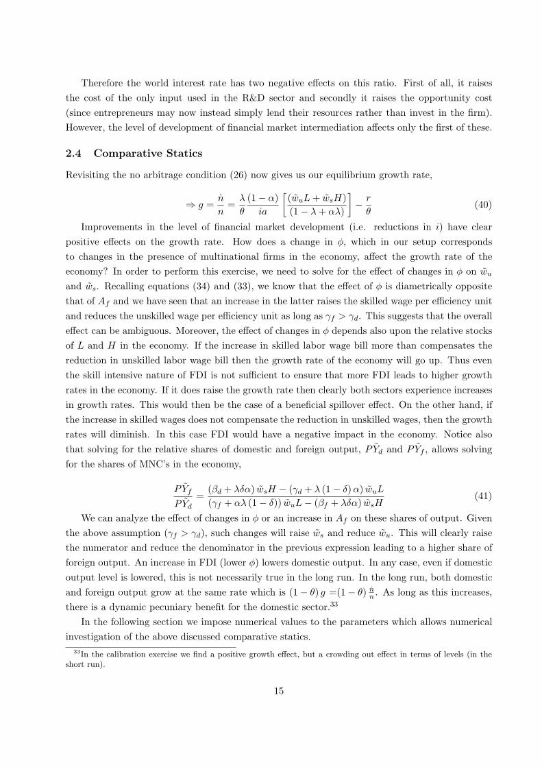
2.4 Comparative Statics

Revisiting the no arbitrage condition (26) now gives us our equilibrium growth rate,

⇒ g =n

n=

λ

θ

(1− α)ia

[(wuL + wsH)(1− λ + αλ)

]− r

θ(40)

Improvements in the level of financial market development (i.e. reductions in i) have clearpositive effects on the growth rate. How does a change in φ, which in our setup correspondsto changes in the presence of multinational firms in the economy, affect the growth rate of theeconomy? In order to perform this exercise, we need to solve for the effect of changes in φ on wu

and ws. Recalling equations (34) and (33), we know that the effect of φ is diametrically oppositethat of Af and we have seen that an increase in the latter raises the skilled wage per efficiency unitand reduces the unskilled wage per efficiency unit as long as γf > γd. This suggests that the overalleffect can be ambiguous. Moreover, the effect of changes in φ depends also upon the relative stocksof L and H in the economy. If the increase in skilled labor wage bill more than compensates thereduction in unskilled labor wage bill then the growth rate of the economy will go up. Thus eventhe skill intensive nature of FDI is not sufficient to ensure that more FDI leads to higher growthrates in the economy. If it does raise the growth rate then clearly both sectors experience increasesin growth rates. This would then be the case of a beneficial spillover effect. On the other hand, ifthe increase in skilled wages does not compensate the reduction in unskilled wages, then the growthrates will diminish. In this case FDI would have a negative impact in the economy. Notice alsothat solving for the relative shares of domestic and foreign output, PYd and PYf , allows solvingfor the shares of MNC’s in the economy,

PYf

PYd

=(βd + λδα) wsH − (γd + λ (1− δ) α) wuL

(γf + αλ (1− δ)) wuL− (βf + λδα) wsH(41)

We can analyze the effect of changes in φ or an increase in Af on these shares of output. Giventhe above assumption (γf > γd), such changes will raise ws and reduce wu. This will clearly raisethe numerator and reduce the denominator in the previous expression leading to a higher share offoreign output. An increase in FDI (lower φ) lowers domestic output. In any case, even if domesticoutput level is lowered, this is not necessarily true in the long run. In the long run, both domesticand foreign output grow at the same rate which is (1− θ) g =(1− θ) n

n . As long as this increases,there is a dynamic pecuniary benefit for the domestic sector.33

In the following section we impose numerical values to the parameters which allows numericalinvestigation of the above discussed comparative statics.

33In the calibration exercise we find a positive growth effect, but a crowding out effect in terms of levels (in theshort run).

15

3 Numerical Simulation

In order to illustrate the qualitative properties of the model discussed in section 2, we calibrate theparameters based on previous econometric and numerical studies and compute the growth ratesimplied by our model. The purpose of the below exercise is to numerically study the growth effectsof FDI, with a focus on identifying the differential growth effects across different levels of financialmarket development.

For this purpose we group countries based on their income levels, and use the correspondinglevels of financial market development. Countries with income levels below $2,000 GDP per capitain 2000 are grouped as “low financially developed” economies, whereas countries with income levelsabove $10,000 GDP per capita are grouped as “high financially developed” economies. Remainingcountries are labelled as “medium financially developed” economies.34 Different measures havebeen used in the literature to proxy for financial market development.35 The broader financialmarket development measures such as the monetary-aggregates as a share of GDP and the privatesector credit extended by financial institutions as a share of GDP capture the extent of financialintermediation; interest rate spreads, on the other hand, capture the cost of intermediation. Giventhat the spread between the lending and borrowing rates better captures the spirit of our model, weprefer it as the measure for the development of the financial markets in the below exercise. We find,however, that the alternative measures of financial market development, including the size of thefinancial market, the share of private sector credit in total banking activity, the overhead costs andthe interest rate spreads, are all highly correlated. This high correlation suggests that the resultsare not limited by the choice of the financial market development proxy.36 Erosa (2001) defines thefinancial intermediation cost as the resources used up per unit of value that is intermediated, whichis the total value of financial assets owned by the financial institutions. Accordingly, he measuresthe financial intermediation cost as the spread between the lending and borrowing rates.37 Theparameter that captures the financial market inefficiencies denoted by, ∆ = i − r, will be proxiedby this measure of intermediation cost. The average spread for the low financially developed(poor) countries, medium financially developed (middle income) countries and the high financiallydeveloped (rich) countries between 2000 and 2003 are 14.5%, 8.5%, and 4.5%, respectively.38

The remaining parameters that are used in the benchmark analysis are taken from previouseconometric and calibration exercises. We start by discussing the production parameters. The

34The real GDP data is PPP adjusted for the year 2000 , and measured in constant US$. Data is obtained fromthe World Development Indicators (World Bank, 2004).

35See Levine et al. (2000), Erosa (2001), Imrohoroglu and Kumar (2003).36The development of the financial markets could alternatively be proxied using broad measures of banking sector

development such as private credit to GDP as in Levine et al (2000) or stock market variables such as capitalizationto GDP as in Levine and Zervos (1998); or as the overhead costs as a share of total loans, following Imrohoroglu andKumar (2003). As mentioned, the different measures are highly correlated.

37See Erosa (2001), pages 306-07 for a more detailed discussion.38We also looked into a breakdown into 5 groups, however the spread value for those countries with income

level between $2000–$4000, $4000–$6000, $6000–$8000 and $8000–$10000 are found to be around 8.5% on average.Therefore, the classification in such smaller grid among the middle income countries does not create variation in thespread. On account of this we define the middle-income range as those covering $2000–$10000 real income per capitain 2000.

16

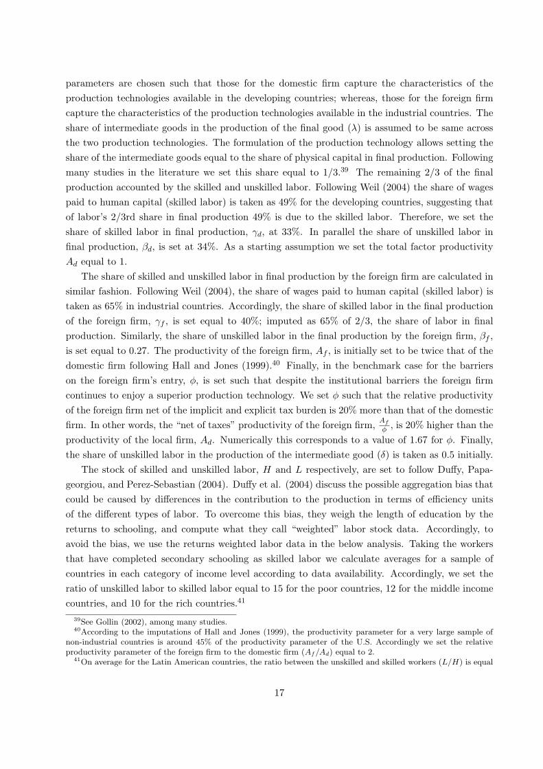
parameters are chosen such that those for the domestic firm capture the characteristics of theproduction technologies available in the developing countries; whereas, those for the foreign firmcapture the characteristics of the production technologies available in the industrial countries. Theshare of intermediate goods in the production of the final good (λ) is assumed to be same acrossthe two production technologies. The formulation of the production technology allows setting theshare of the intermediate goods equal to the share of physical capital in final production. Followingmany studies in the literature we set this share equal to 1/3.39 The remaining 2/3 of the finalproduction accounted by the skilled and unskilled labor. Following Weil (2004) the share of wagespaid to human capital (skilled labor) is taken as 49% for the developing countries, suggesting thatof labor’s 2/3rd share in final production 49% is due to the skilled labor. Therefore, we set theshare of skilled labor in final production, γd, at 33%. In parallel the share of unskilled labor infinal production, βd, is set at 34%. As a starting assumption we set the total factor productivityAd equal to 1.

The share of skilled and unskilled labor in final production by the foreign firm are calculated insimilar fashion. Following Weil (2004), the share of wages paid to human capital (skilled labor) istaken as 65% in industrial countries. Accordingly, the share of skilled labor in the final productionof the foreign firm, γf , is set equal to 40%; imputed as 65% of 2/3, the share of labor in finalproduction. Similarly, the share of unskilled labor in the final production by the foreign firm, βf ,is set equal to 0.27. The productivity of the foreign firm, Af , is initially set to be twice that of thedomestic firm following Hall and Jones (1999).40 Finally, in the benchmark case for the barrierson the foreign firm’s entry, φ, is set such that despite the institutional barriers the foreign firmcontinues to enjoy a superior production technology. We set φ such that the relative productivityof the foreign firm net of the implicit and explicit tax burden is 20% more than that of the domesticfirm. In other words, the “net of taxes” productivity of the foreign firm, Af

φ , is 20% higher than theproductivity of the local firm, Ad. Numerically this corresponds to a value of 1.67 for φ. Finally,the share of unskilled labor in the production of the intermediate good (δ) is taken as 0.5 initially.

The stock of skilled and unskilled labor, H and L respectively, are set to follow Duffy, Papa-georgiou, and Perez-Sebastian (2004). Duffy et al. (2004) discuss the possible aggregation bias thatcould be caused by differences in the contribution to the production in terms of efficiency unitsof the different types of labor. To overcome this bias, they weigh the length of education by thereturns to schooling, and compute what they call “weighted” labor stock data. Accordingly, toavoid the bias, we use the returns weighted labor data in the below analysis. Taking the workersthat have completed secondary schooling as skilled labor we calculate averages for a sample ofcountries in each category of income level according to data availability. Accordingly, we set theratio of unskilled labor to skilled labor equal to 15 for the poor countries, 12 for the middle incomecountries, and 10 for the rich countries.41

39See Gollin (2002), among many studies.40According to the imputations of Hall and Jones (1999), the productivity parameter for a very large sample of

non-industrial countries is around 45% of the productivity parameter of the U.S. Accordingly we set the relativeproductivity parameter of the foreign firm to the domestic firm (Af/Ad) equal to 2.

41On average for the Latin American countries, the ratio between the unskilled and skilled workers (L/H) is equal

17

The remaining parameters are α = 0.91, r = 0.05 and P = 1. Based on the work of Basu (1996),the mark-up is assumed to be 10%, and hence the value of the reciprocal of (1+mark-up) is givenby α = 0.91. The risk free interest rate is assumed to be 5%. The price of the final good is taken asthe numeraire. The cost of introducing a new variety of product, a, is taken as the free parameter,which is calibrated to allow for realistic growth figures for each set of income group. Finally, theparameter capturing the ease of developing new variety of products, θ, is limited by other parameterchoices given the following formulation: θ = 1 − (λ ∗ (1 − α)/α). Table 1 summarizes the mainparameters used in the numerical exercise.

Table 1: Benchmark Parameter ValuesCommon parameters 2Ad = Af , φ = 1.67 λf = 0.33 λd = 0.33

r = 0.05, α = 0.91 βf = 0.27, γf = 0.40 γd = 0.33, βd = 0.44Finan. Dev. Level Low (∆ = 0.145) Medium (∆ = 0.085) High (∆ = 0.045)Factor Endowment L=15H L=2H L=10H

The benchmark solution for the growth rates are reported in Table 2, column I. The results foreach financial market development level suggest that the implied growth rates by the above exerciseare very close to the observed growth rates. For the period 1976-2003 the average annual growth ratefor the low financially developed economies was around 0.1%, for the medium financially developedeconomies was around 2.0%, and for the high financially developed economies was around 2.3%.42,

43

Upon solving the benchmark case, we look into the growth effects of increased FDI inflows,keeping all else constant. The technology effects of FDI are captured through the net productivityparameter of the foreign firm. An increase in Af or a decrease in φ both capture an increase inFDI. In imputing the effects of FDI on the net productivity parameter, we refer to Coe, Helpmanand Hoffmaister (1997). Analyzing the spillovers from foreign R&D activity on the Southern totalfactor productivities (TFP) Coe, Helpman and Hoffmaister (1997) regress the domestic TFP of theSouthern economies on foreign R&D stock, among several other variables. This regression allowsidentification of the foreign R&D elasticity of TFPs. In the benchmark regression, Coe and Helpmanreport this elasticity to be at the range of 0.73-0.75. However they further argue that, although thisregression shows positive and significant effects of the foreign R&D stock on domestic TFP’s, theyprefer the specification which includes fixed effects and time trends.44 In this preferred regressionthey report the elasticity as 0.058. In the following analysis, we use Coe and Helpman (1997)’sfindings as the benchmark in quantifying the effects of FDI on the net productivity parameters. We

to 10; for a group of countries that include Latin America, Central America, and the East Asia and Pacific region theaverage increases to 12. The ratio for a sample of developed countries, including the US, European Union economies,Canada and Japan, is found to be 5.

42These growth rates were calculated using World Development Indicators (World Bank, 2004) data on the realGDP per capita, PPP adjusted and measured in US$.

43The results provide realistic values for the remaining variables that are solved, specifically the skill premium andthe relative output between domestic and foreign production.

44The referred to estimation results in Coe, Helpman and Hoffmaister (1997) are reported in Table 2, page 142. Thestandard regressions referred to are regressions (i) and (iii). The regression specification preferred by Coe, Helpmanand Hoffmaister (1997) is regression (x) reported in the same table.

18

make the assumption that, given the nature of FDI – which is composed of both foreign capital andtechnology and know-how – an increase in foreign R&D is fully reflected in the FDI flows. In otherwords, we take the effects of a 1% increase in foreign R&D on the Southern TFP as equivalent tothe effects of a 1% increase in FDI. Following Coe, Helpman and Hoffmaister (1997), we set theFDI elasticity of the foreign firm TFP equal to 0.058, which implies that a 1% increase in FDIflows increases the net foreign firm TFP by 0.058%. In the above discussion of the parameterswe discussed that the net foreign firm productivity parameter, Af

φ , is set equal to 21.67 . Therefore,

according to the FDI elasticity of TFP, a 1% increase in FDI inflows increases this net productivityparameter by 0.058%, to 2

1.669 .45

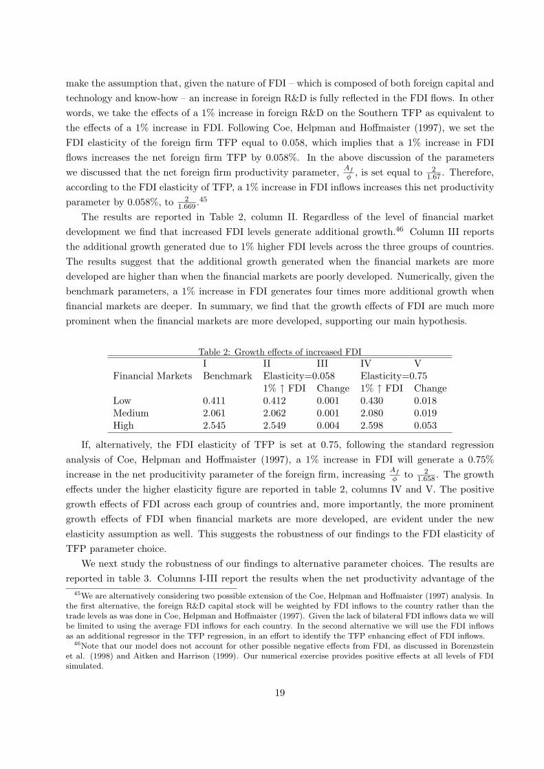
The results are reported in Table 2, column II. Regardless of the level of financial marketdevelopment we find that increased FDI levels generate additional growth.46 Column III reportsthe additional growth generated due to 1% higher FDI levels across the three groups of countries.The results suggest that the additional growth generated when the financial markets are moredeveloped are higher than when the financial markets are poorly developed. Numerically, given thebenchmark parameters, a 1% increase in FDI generates four times more additional growth whenfinancial markets are deeper. In summary, we find that the growth effects of FDI are much moreprominent when the financial markets are more developed, supporting our main hypothesis.

Table 2: Growth effects of increased FDII II III IV V

Financial Markets Benchmark Elasticity=0.058 Elasticity=0.751% ↑ FDI Change 1% ↑ FDI Change

Low 0.411 0.412 0.001 0.430 0.018Medium 2.061 2.062 0.001 2.080 0.019High 2.545 2.549 0.004 2.598 0.053

If, alternatively, the FDI elasticity of TFP is set at 0.75, following the standard regressionanalysis of Coe, Helpman and Hoffmaister (1997), a 1% increase in FDI will generate a 0.75%increase in the net producitivity parameter of the foreign firm, increasing Af

φ to 21.658 . The growth

effects under the higher elasticity figure are reported in table 2, columns IV and V. The positivegrowth effects of FDI across each group of countries and, more importantly, the more prominentgrowth effects of FDI when financial markets are more developed, are evident under the newelasticity assumption as well. This suggests the robustness of our findings to the FDI elasticity ofTFP parameter choice.

We next study the robustness of our findings to alternative parameter choices. The results arereported in table 3. Columns I-III report the results when the net productivity advantage of the

45We are alternatively considering two possible extension of the Coe, Helpman and Hoffmaister (1997) analysis. Inthe first alternative, the foreign R&D capital stock will be weighted by FDI inflows to the country rather than thetrade levels as was done in Coe, Helpman and Hoffmaister (1997). Given the lack of bilateral FDI inflows data we willbe limited to using the average FDI inflows for each country. In the second alternative we will use the FDI inflowsas an additional regressor in the TFP regression, in an effort to identify the TFP enhancing effect of FDI inflows.

46Note that our model does not account for other possible negative effects from FDI, as discussed in Borenzsteinet al. (1998) and Aitken and Harrison (1999). Our numerical exercise provides positive effects at all levels of FDIsimulated.

19

foreign firm relative to the domestic firm is reduced from 20% to 15%. The qualitative resultsregarding the growth effects of FDI remain robust to the change in the extent of productivityadvantage of the foreign firm. Regardless of the technology gap between the foreign and thedomestic firm higher FDI inflows generate higher growth benefits to the host country when thelocal financial markets are much more developed. Columns IV-VI report the results when the netproductivity advantage of the foreign firm increases to 25%, and the relative labor endowments ineach group of countries are further changed to check for the robustness of the results to the factorendowments of the host economies. The ratio of the unskilled labor to skilled labor is increased to 20for the low financially developed economies, to 18 for the medium financially developed economies,and decreased to 3 for the economies with well developed financial markets.47 As in columns I-IIIour findings remain robust to alternative choices of relative factor endowments. As is evident incolumn VI, growth effects of FDI are much higher when local financial markets are deeper. Table 3suggests that the qualitative results are robust to changes in the technology gap between the localand foreign firm, as well as the factor endowment of the host country.

Table 3: Growth effects of increased FDI, Robustness of ResultsI II III IV V VI

Financial Markets Af

φ = 21.71 ε=0.75 Af

φ = 21.60 ε=0.75

1% ↑ FDI Change 1% ↑ FDI ChangeLow 0.665 0.679 0.014 0.313 0.330 0.017Medium 1.858 1.894 0.036 2.298 2.342 0.044High 2.266 2.310 0.044 2.345 2.623 0.278

We also considered the effects of an improvement in the financial markets, all else constant.Setting the ratio of unskilled to skilled labor (L/H) equal to 9, and keeping all parameters constant(including the free parameter ”a”) we allow for improvements in the financial market developmentof the economy. When financial markets improve from the level of the low to the medium developed,i.e., ∆ changes from 14.5 to 8.5 percent, all else constant the growth rate increases from -0.07 to2.19 percent. Similarly, when the financial markets improve from the level of the medium to thehigh level of financial market development level, i.e., ∆ changes from 8.5 to 4.5 percent, the growthrate of the economy increases from 2.19 to 5.29 percent. The same effect is observed for alternativeendowment assumptions, suggesting that the positive growth effects of improvementsin the financialmarket development are robust to parameter assumptions as discussed in the comparative staticssection above.

4 Conclusions

to be written....47Duffy, et al. (2004) in fact report the relative unskilled to skilled labor ratios as 20, 16, and 3 for the poorly,

medium and well developed financial market economies, respectively.

20

5 References

Aghion P., P. Bacchetta, R. Ranciere, and K. Rogoff, 2005. “Productivity Growth and theExchange Rate Regime: The Role of Financial Development,” mimeo.

Aghion, P. and P. Howitt, 1999. Endogenous Growth Theory, Cambrigde, Ma: MIT Press.

Aghion, P., P. Howitt, and D. Mayer-Foulkes, 2005. “The Effect of Financial Developmenton Convergence: Theory and Evidence,” Quarterly Journal of Economics120, 173-222.

Alfaro, L., A. Chanda, S. Kalemli-Ozcan and S. Sayek, 2004. “FDI and Economic Growth,The Role of Local Financial Markets,” Journal of International Economics 64, 113-134.

Alfaro, L. and A. Rodriguez-Clare, 2004. “Multinationals and Linkages: Evidence from LatinAmerica,” Economia 4, 113-170.

Barba Navaretti, G. and A. Venables, 2004. Multinational Firms in the World Economy.Princeton University Press.

Basu, S., 1996. “Procyclical Productivity: Increasing Returns or Cyclical Utilization,” QuarterlyJournal of Economics 111, 719-751.

Blomstrom, M. and A. Kokko, 1998. “Multinational Corporations and Spillovers,” Journalof Economic Surveys 12, 247-277.

Borensztein, E., J. De Gregorio, and J-W. Lee, 1998. “How Does Foreign Direct Invest-ment Affect Economic Growth?” Journal of International Economics 45, 115-135.

Boyd, J. H., E. C. Prescott, 1986. “Financial Intermediary Coalitions,” Journal of EconomicTheory 38, 211–232.

Burnstein, A. and A. Monge-Naranjo, 2005. “Aggregate Consequences of International Firmsin Developing Countries,” mimeo.

Cardoso, F. and E. Faletto, 1970. Dependency and Development in Latin America. Berkeley,CA: University of California Press.

Carkovic, M. and R. Levine, 2002. “Does Foreign Direct Investment Accelerate Economic Growth?”University of Minnesota, Working Paper.

Chang, R., L. Kaltani and N. Loayza, 2005. “Openness Can be Good for Growth: The Roleof Policy Complementarities,” mimeo.

Coe, D. T. and E. Helpman, 1995. “International R&D Spillovers,”European Economic Re-view 39, 859-887.

Coe, D.T., E. Helpman and A. Hoffmaister, 1997. “North-South R&D Spillovers,” EconomicJournal 107, 134-149.

21

Diamond, D., 1984. “Financial Integration and Delegated Monitoring,” Review of EconomicStudies 51, 393-419.

Duffy, J., C. Papageorgiou and F. Perez-Sebastian, 2004. “Capital-Skill Complementarity?Evidence From a Panel of Countries,” The Review of Economics and Statistics 86, 327-344.

Dunning, J.H., 1981. International Production and the Multinational Enterprise. London, U.K.:George Allen and Unwin.

Durham, K.B.J.B., 2004. “Absorptive Capacity and the Effects of Foreign Direct Investmentand Equity Foreign Portfolio Investment on Economic Growth,” European Economic Review48, 285-306.

Edwards, S. and C. Vegh, 2004. “Banks and Macroeconomic Disturbances under Predeter-mined Exchange Rates,” Journal of Monetary Economics 40, 239-278.

Erosas, Andres, 2001, “Financial Intermediation and Occupational Choice in Development,”Review of Economic Dynamics, 4:303-334.

Galor, O., and J. Zeira, 1993. “Income Distribution and Macroeconomics,” Review of Eco-nomic Studies 60, 35-52.

Gollin, D. 2002. “Getting Income Shares Right,” Journal of Political Economy 110, 458-474.

Goldsmith, R. W., 1969. Financial Structure and Development, New Haven, Connecticut: YaleUniversity Press.

Greenwood, J., B. Jovanovic, 1990. “Financial Development, Growth and the Distribution ofIncome,” Journal of Political Economy 98, 1076–1107.

Grossman, G., and E. Helpman, 1992. Innovation and Growth in the Global Economy. Cam-bridge: MIT Press.

Hanson, G. H., 2001. “Should Countries Promote Foreign Direct Investment?” G-24 DiscussionPaper No. 9. New York: United Nations.

Hall, R. E. and C. Jones, 1999. “Why Do Some Countries Produce So Much More Output perWorker than Others?” The Quarterly Journal of Economics 114, 83–116.

Helpman, E. and P. Krugman, 1985. Market Structure and Foreign Trade: Increasing Re-turns, Imperfect Competition, and the International Economy. Cambridge: MIT Press.

Hobday, M. 1995. Innovation in East Asia: The Challenge to Japan. Cheltenham: EdwardElgar.

Hermes, N., Lensink, R., 2003. “Foreign Direct Investment, Financial Development and Eco-nomic Growth,” Journal of Development Studies 40, 142-163.

22

Hirschman, A., 1958. it The Strategy of Economic Development. New Haven: Yale UniversityPress.

Holmstrom, B. and J. Tirole, 1993. “Market Liquidity and Performance Monitoring,” Jour-nal of Political Economy 101, 678-709.

Imrohoroglu, A. and K. B. Kumar, 2004. “Intermediation Costs and Capital Flows,” Reviewof Economic Dynamics7, 586-612.

Javorcik, B. S., 2004. “Does Foreign Direct Investment Increase the Productivity of DomesticFirms? In Search of Spillovers Through Backward Linkages,” American Economic Review94, 605-627.

Kindleberger, C. P., 1969. American Business Abroad. New Haven, CT: Yale University Press.

King, R., R. Levine, 1993a. “Finance and Growth: Schumpeter Might be Right,” QuarterlyJournal of Economics 108, 717–738.

King, R., R. Levine, 1993b. “Finance, Entrepreneurship and Growth: Theory and Evidence,”Journal of Monetary Economics 32, 513–542.

Lall, S., 1980. “Vertical Inter-Firm Linkages in LDCs: An Empirical Study,” Oxford Bulletin ofEconomics and Statistics 42, 203-206.

Larrain, F., L. Lopez-Calva, and A. Rodriguez-Clare, 2000. “Intel: A Case Study of For-eign Direct Investment in Central America,” Center for International Development, HarvardUniversity Working Paper No. 58.

Levine, R., N. Loayza, and T. Beck, 2000. “Financial Intermediation and Growth: Causal-ity and Causes,” Journal of Monetary Economics 46, 31–77.

Levine, R. and S. Zervos, 1998. “Stock Markets, Banks and Economic Growth,” AmericanEconomic Review 88, 537–558.

Lipsey, R. E., 2002. “Home and Host Country Effects of FDI,” NBER Working Paper 9293.

Markusen. J. and A.J. Venables, 1999. “Foreign Direct Investment as a Catalyst for Indus-trial Development,” European Economic Review 43, 335-338.

Parikh, K. S. (ed.), 1997. India Development Report. Delhi: Oxford University Press.

Perez, C., 2000. “Empresa de Technologıa con cautela en 2002,” El Financiero, January 7-13.

Rodrıguez-Clare, A., 1996. “Multinationals, Linkages and Economic Development,” AmericanEconomic Review 86, 852-873.

Spar, D., 1998. “ Attracting High Technology Investment: Intel’s Costa Rica Plant,” World BankOccasional Paper 11.

23

Weil, David, 2004, Economic Growth, Addison-Wesley.

Xu, B., 2000. “Multinational Enterprises, Technology Diffusion, and Host Country ProductivityGrowth,” Journal of Development Economics 62, 477-493.

24

A Calculating Output of Final Goods Sector

Using the cost functions for the domestic, foreign and intermediate goods sector and Shepard’sLemma, we can derive the equilibrium conditions in the labor market. The demand for skilled andunskilled labor by the domestic sector are given, respectively, by the following expressions,

∂c(wu, ws, px, Yd)∂wu

=A−1

d β−βdd

(1− γd − βd)(1−γd−βd)βdw

βd−1u wγd

s p1−γd−βdx n

(1−γd−βd)(α−1)

α Yd = Ld (42)

∂c(wu, ws, px, Yd)∂ws

=A−1

d β−βdd

(1− γd − βd)(1−γd−βd)γdw

βdu w

γd−1s p1−γd−βd

x n(1−γd−βd)(α−1)

α Yd = Hd (43)

In the foreign sector,

∂c(wu, ws, px, Yf )∂wu

=φ(τ)A−1

f β−βf

f γ−γf

f

(1− γd − βd)(1−γd−βd)βfw

βf−1u w

γfs p

(1−γf−βf )

x n(1−γf−βf )(α−1)

α Yf = Lf (44)

∂c(wu, ws, px, Yf )∂ws

=φ(τ)A−1

f β−βf

f γ−γf

f

(1− γd − βd)(1−γd−βd)γfw

βfu w

γf−1s p

(1−γf−βf )

x n(1−γf−βf )(α−1)

α Yf = Hf (45)

And in the intermediate good sector,

∂c(wu, ws, x)∂wu

= δ−δ(1− δ)−(1−δ)(δ)wδ−1u w(1−δ)

s x = Lx (46)

∂c(wu, ws, x)∂ws

= δ−δ(1− δ)−(1−δ)(1− δ)wδuw(−δ)

s x = Hx (47)

Using the equilibrium conditions in the final good sector, (9) and (10), one can rearrangeequation (31) and (32) as

βdPYd

wu+

βfPYf

wu+

δαpxxn

wu= L

Using the expression for the total revenues for the intermediate good sector as a share of totaloutput, (17), we can rewrite the equilibrium condition for unskilled labor as,

⇒ [βd + δα (1− γf − βf )]PYd

wu+

[βf + δα (1− γd − βd)]PYf

wu= L (48)

Similarly, for skilled labor,

⇒ [γd + (1− δ)α (1− γf − βf )]PYd

ws+

[γf + (1− δ)α (1− γd − βd)]PYf

ws= H (49)

25

The two equations above also shed light on the possible values for θ. The final sector productionfunctions are Cobb-Douglas which means that labor shares are constant. This must mean that ifwi = wi/n(1−α)/λα (i = u, s) and Yj = Yj/n1−θ (j = d, f) then it must be that case that,

λ (1− α)α

= 1− θ

Therefore from the labor allocation equation (48) we have

(βd + λδα) PYd

wu+

(βf + λδα)PYf

wu= L (50)

by similar reasoning using (49),

(γd + λ(1− δ)α) PYd

ws+

(γf + λ(1− δ)α) PYf

ws= H (51)

Rearranging the equilibrium condition for labor, (50), and inserting it in the equilibrium condi-tion for human capital, (51), and using (γf − γd) = (βd − βf ),48 we obtain the following expressionfor foreign production,

PYf =(βd + λδα) wsH − (γd + λ (1− δ) α) wuL

(1− λ + αλ) (βd − βf )(52)

and the following expression for the domestic production,

PYd =(γf + αλ (1− δ)) wuL− (βf + λδα) wsH

(1− λ + αλ) (βd − βf )(53)

B Modelling Financial Markets

In this appendix we present a bare-bones model of imperfect financial markets using the costlystate verification approach. The model is adapted from Levine and King (1993).49 As in theirmodel we assume individuals have equal financial wealth which is a claim on profits of a diversifiedportfolio of firms engaged in innovative activity. Some individuals do have the ability to manageinnovation but this does not lead them to accumulate different levels of wealth from the rest ofindividuals in the economy. These potential entrepreneurs have the ability to successfully managea project with probability α. These abilities are unobservable to both the entrepreneur and thefinancial intermediary. However, the actual capability of such an individual to manage a project

48In particular, we use (γf + λ (1− δ) α) (βd + λδα) − (γd + λ (1− δ) α) (βf + λδα) = (1− λ + αλ) (βd − βf )to derive the condition for the foreign production. For the domestic production, we use((1− λ + αλ) (βd − βf ) + (βf + λδα) (γd + λ (1− δ) α)) = (βd + λδα) (γf + αλ (1− δ)) .

49see Aghion, Howitt and Mayer-Foulkes (2005) for an alternative modelling strategy for imperfect financial marketsin an endogenous growth models. In their model, entrepreneurs can pay an upfront cost and defraud the lenders.Incentive compatibility constraints and arbitrage conditions then leads to an upper bound on how much is actuallyinvested in new innovations which is lower than the optimal investment amount. The gap between the two is aninverse function of the degree of creditor protection. Their model seems more suited to “quality ladder” Schumpeterianmodels whereas the King and Levine structure is more easily incorporated into a product variety setup such as ours.

26

can be ascertained at a cost, F .50 The main two differences are the following. First, consistent withour setup, we use capital in the R&D sector instead of labor. The second difference is related to ourassumption regarding the structure of verification costs. We assume these costs to be proportionalto the set up costs for any project. The main advantage of this approach is that it allows us to retainthe balanced growth properties of the model while allowing in principle to make total verificationcosts decreasing in the level of overall technology and hence in the level of development.51 Thereforeone could argue that our setup relates automatically more efficient financial markets to higher levelsof development.52

We depart from the main text in that now R&D projects are potentially risky and there is aprobability α of the project being run successfully. Which potential entrepreneur will manage aproject successfully is unknown both to the entrepreneur and the intermediary. The intermediarycan spend an amount F to reduce the uncertainty regarding the project’s outcome. Further wepostulate the following structure on F :

F = fra

nθ(54)

Therefore since setup costs require anθ units of K then the cost of verification simply is propor-

tional to total setup costs and f represents that factor of proportionality. While not necessary forour model, it seems intuitive that f should be less than 1 - verification costs are likely to be lowerthan setup costs.

If the value of a successful project is q then, with a competitive intermediation sector, inequilibrium we must have,53

αq = F

The value of a successful project is simply the present discounted value of profits (v) minus theset up costs (η). Therefore the above condition can be rewritten as,

a(v − η) = F

Further from our model we had setup costs for each blueprint to be ranθ

54

⇒ α(v − ra

nθ

)= F (55)

In our earlier model we had the condition that v = ranθ due to free entry and exit. However, now

since returns to investment are uncertain and the financial intermediaries face verification costs50Obviously entrepreneurs cannot evaluate themseleves and credibly communicate the results to others.51Indeed King and Levine (1993) suggest this modification as a potentially useful extension of their model (pp

518).52The objective of our paper, as mentioned, is not to model the relation between financial markets and development

but instead the role of financial markets in allowing an economy to reap the benefits of potential FDI spillovers.53Of course in the background we assume that for an intermediary it is better to do this evaluation rather than

simply lending the money and not incurring the verification cost.

54Since the cost of imperfections is being explicitly derived, we know longer impose the ∆.

27

we no longer can impose this condition. On the other hand we still have the standard arbitragecondition from equation (19),

π

v+

v

v= r (56)

Substituting equation (54) in equation (55), we continue to get as in the main modell

v

v= −θ

n

n

Now we can combine this with the previous equation to get,

π

v− θ

n

n= r

In our model the per intermediate firm operating profit was (see equation(18)

πi =(1− α) P

n[(1− γd − βd) Yd + (1− γd − βf ) Yf ]

Therefore

1v

{(1− α) P

n[(1− γd − βd) Yd + (1− γd − βf )Yf ]

}− θ

n

n= r

Noting that

v =f

αr

a

nθ+

ra

nθ

⇒ 1

ra(

fα + 1

){

(1− α) P[(1− γd − βd) Yd + (1− γd − βf ) Yf

]}− θ

n

n= r

where Yi = Yi/n1−θ.

Thus we have an expression for the growth rate similar to the one derived in the main text,

g =n

n=

λ

θ

(1− τ) (1− α)

ra(

fα + 1

)[(wuL + wsH)(1− λ + αλ)

]− r

θ

Of course, what was earlier represented in the main text by i can now be substituted byr(

fα + 1

). In practice f

α is likely to be unobservable across countries. Therefore in the numerical

exercises, when we use the spread, ∆ = i − r, theoretically, we are measuring r fα . Therefore a

higher spread has the same effect as a higher verification costs. Further, for every unique f, givenr and α, there is a unique value of ∆. Therefore using the spread between lending and borrowingrates serves as a convenient proxy for verification costs.

28