Embed Size (px)
Citation preview

Formal definitions of programming languages as a basisfor compiler constructionHemerik, C.
DOI:10.6100/IR55705
Published: 01/01/1984
Document VersionPublisher’s PDF, also known as Version of Record (includes final page, issue and volume numbers)
Please check the document version of this publication:
• A submitted manuscript is the author's version of the article upon submission and before peer-review. There can be important differencesbetween the submitted version and the official published version of record. People interested in the research are advised to contact theauthor for the final version of the publication, or visit the DOI to the publisher's website.• The final author version and the galley proof are versions of the publication after peer review.• The final published version features the final layout of the paper including the volume, issue and page numbers.
Link to publication
General rightsCopyright and moral rights for the publications made accessible in the public portal are retained by the authors and/or other copyright ownersand it is a condition of accessing publications that users recognise and abide by the legal requirements associated with these rights.
• Users may download and print one copy of any publication from the public portal for the purpose of private study or research. • You may not further distribute the material or use it for any profit-making activity or commercial gain • You may freely distribute the URL identifying the publication in the public portal ?
Take down policyIf you believe that this document breaches copyright please contact us providing details, and we will remove access to the work immediatelyand investigate your claim.
Download date: 28. Aug. 2018
FORMAL DEFINITIONS OF PROGRAMMING LANGUAGES
AS A BASIS FOR COMPILER CONSTRUCTION
C. HEMERIK

FORMAL DEFINITIONS OF PROGRAMMING LANGUAGES
AS A BASIS FOR COMPILER CONSTRUCTION

Druk: Dissertatie Drukkerij Wibro, Helmond. Telefoon .04920-23981.

FORMAL DEFINITIONS OF PROGRAMMING LANGUAGES
AS A BASIS FOR COMPILER CONSTRUCTION
PROEFSCHRIFT
TER VERKRIJGING VAN DE GRAAD VAN DOCTOR IN DE
TECHNISCHE WETENSCHAPPEN AAN DE TECHNISCHE
HOGESCHOOL EINDHOVEN, OP GEZAG VAN DE RECTOR
MAGNIFICUS, PROF.DR. S.T.M. ACKERMANS, VOOR
EEN COMMISSIE AANGEWEZEN DOOR HET COLLEGE
VAN DEKANEN IN HET OPENBAAR TE VERDEDIGEN OP
DINSDAG 15 MEI 1984 TE 16.00 UUR
DOOR
CORNELIS HEMERI K
GEBOREN TE LEIDEN

Dit proefschrift is goedgekeurd
door de promotoren
prof.dr. F.E.J. Kruseman Aretz
en
prof. dr. E.W. Dijkstra

CONTENTS
0. Introduetion
0. I. Background
0.2. Subject of the thesis 3
0.3. Some notational conventions 6
I. On formal definitions of programming languages 8
2. Formal syntax and the kernel language 13
2.0. Introduetion 13
2.1. Context-free grammars 14
2.1.1. Definition of context-free grammar and related notions 14
2.1.2. Presentation 16
2.1.3. Implementation concerns 18
2.2. Attribute grammars 21
2.2.0. Introduetion 21
2.2.1. Definition of attribute grammar and related notions 23
2.2.2. Presentation 30
2.2.3. Example: Satisfiable Boolean Expressions 32
2.2.4. Implementation concerns 37
2.3. Formal syntax of the kernel language 40
2.3.1. A context-free grammar for the kernel language 40
2.3.2. An attribute grammar for the kernel language 43
3. Predicate transfarmer semantics for the kernel language 50
3.0. Introduetion 50
3.1. Some lattice theory 54
3.1.1. General definitions 54
3.1.2. Strictness 60
3.1.3. Monotoniçity 61
3.1.4. Conjunctivity and disjunctivity 62
3.1.5. Continuity 63
3.1.6. Fixed points 70
3.1.7. Fixed point induction 72

3.2. The condition transfermers wp and wlp 74
3.2.0. Introduetion 74
3. 2. I. Conditions 75
3.2.2. The logic D 79
3.2.3. The ccl's of conditions and condition transfermers 82
3.2.4. Definitions and some properties of wp and wlp 84,
3.3. Logies for partial and total correctness 100
4. Blocks and procedures
4.0. Introduetion 107
4.1. Blocks 109
4.1.0. Introduetion 109
4. l.I. Blocks without redeclaration 109
4.1.2. Substitution in statements 114
4.1.3. Blocks with the possibility of redeclaration 117
4.1.4. Proof rules 118
4.2. Abstraction and application 121
4.2.0. Introduetion 121
4. 2. I. Syntax 121
4.2.2. Semantics 124
4.2.3. Proof rules 126
4.3. Parameterless recursive procedures 131
4.3.0. Introduetion 131
4.3. I. Semantics 131
4.3.2. Proof rules 140
4.3.2.1. Proof rules for partial correctness 141
4.3.2.2. Proof rules for total correctness 144
4.3.2.3. A note on the induction rules and their proofs 148
4.4. Recursive procedures with parameters 150
4.4.0. Introduetion 150
4.4. I. Syntax 150
4.4.2. Semantics 153
4.4.3. Proof rules 157
4.4.3.1. Proof rules for partial correctness 157
4.4.3.2. Proof rules for total correctness 163

5. Some aspeets of the definition of the target language
5.0. Introduetion
5. I. Informal deseription of TL
5.2. Version I : Condition transfarmer semantics of TL
5.3. Version 2: Introduetion of program store
5.4. Version 3: Introduetion of return stack
5.5. Version 4: Derivation of an interprete.r
6. Epilogue
Appendix A. Proofs of some lemmas
Appendix B. Collected definition of the souree language
Index of definitions
References
Samenvatting
Curriculum vitae
167
167
169
17 I
182
185
188
193
195
199
212
215
220
223
0. I • Background
CHAPTER 0
INTRODUClïON
I •
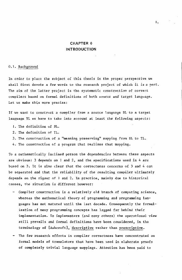
In order to place the subject of this thesis in the proper perspective we
shall first devote a few words to the research project of which it is a part.
The aim of the latter project is the systematic construction of correct
compilers based on formal definitions of both souree and' target language.
Let us make this more precise:
If we want to construct a compiler from a souree language SL to a target
language TL we have to take into account at least the following aspects:
1. The definition of SL.
2. The definition of TL.
3. The construction of a "meaning preserving" mapping from SL to TL.
4. The construction of a program that realizes that mapping.
To a mathematically inclined person the dependencies between these aspects
are obvious: 3 depends on I and 2, and the specifications used in 4 are
based on 3. It is also clear that the correctness concerns of 3 and 4 can
be separated and that the reliability of the resulting compiler ultimately
depends on the rigour of I and 2. In practice, mainly due to bistorical
causes, the situation is different.however:
Compiler construction is a relatively old branch of computing science~
whereas the mathematica! theory of programming and programming lan
guages bas not matured until the last decade. Consequently the formal
ization of many programming concepts has lagged far bebind their
implementation. To implementers (and many others) the operational view
still prevails and formal definitions have been considered, in the
terminology of [Ashcroft], descriptive rather than prescriptive.
The few research efforts in compiler correctness have concentrated on
formal roodels of translatars that have been used in elaborate proofs
of completely trivial language mappings. Attention has been paid to
2.
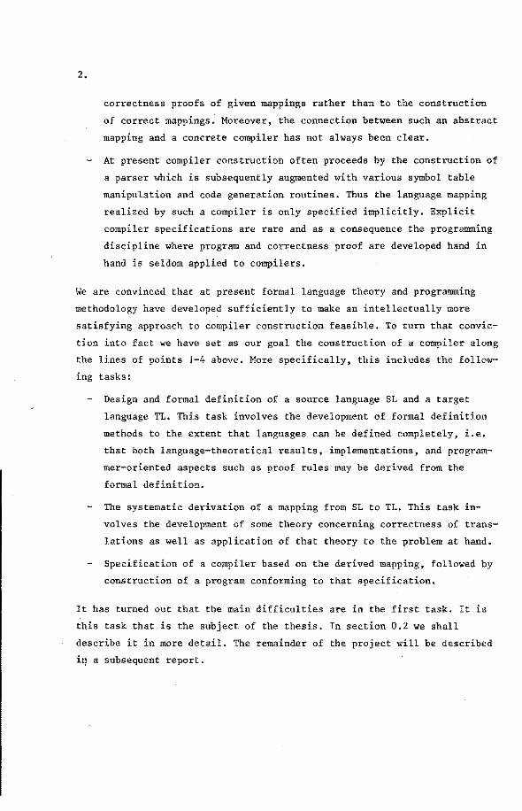
correctness proofs of given mappings rather than to the construction
of correct mappings. Moreover, the conneetion between such an abstract
mapping and a concrete compiler has not always been clear.
At present compiler construction often proceeds by the construction of
a parser which is subsequently augmented with various symbol table
manipulation and code generation routines. Thus the language mapping
realized by such a compiler is only specified implicitly. Explicit
compiler specifications are rare and as a consequence the programming
discipline where program and correctness proof are developed hand in
hand is seldom applied to compilers.
We are convineed that at present formàl language theory and programming
methodology have developed sufficiently to make an intellectually more
satisfying approach to compiler construction feasible. To turn that convic
tion into fact we have set as our goal the construction of a compiler along
the lines of points 1-4 above. More specifically, this includes the follow
ing tasks:
Design and formal definition of a souree language SL and a target
language TL. This task involves the development of formal definition
methods to the extent that languages can be defined completely, i.e.
that both language-theoretical results, implementations, and program
mer-oriented aspects such as proof rules may be derived from the
formal definition.
The systematic derivation of a mapping from SL to TL. This task in
volves the development of some theory concerning correctness of trans
lations as well as application of that theory to the problem at hand.
Specificatien of a compiler based on the derived mapping, foliowed by
construction of a program conforming to that specification.
It has turned out that the main difficulties are in the first task. It is
this task that is the subject of the thesis. In section 0.2 we shall
describe it in more detail. The remainder of the project will be described
iq a subsequent report.

0.2. Subjeèt of the thesis
As already mentioned, the subject of this thesis is the design and. formal
definition of a souree language SL and a target language TL, tagether with
the development of supporting definition methods. Our aim is to obtain
language definitions which present programs as mathematica! objects free
of reference or commitment to particular implementations, but which are
also sufficiently complete and precise to derive correct implementations
from. From the background sketched insection 0.1 it will be clear that
this thesis should not be considered as an isolated and self-contained
study on formal language definition. The major part of the work reported
bere is intended as theoretica! foundation of the aforementioned work on
compiler correctness. We emphasize this background because it may no~ be
obvious from the outer appearance of this thesis, although it is of sig
nificant influence on its subject matter, e.g. in the following respects:
This thesis is concerned neither with development of general defini
tion methods, nor with general theory concerning such methods.
3.
Rather it is concerned with development of formal tools which are bath
theoretically well-founded and practically usable. The mathematica!
apparatus needed for this purpose is only developed as far as necessary.
Most work on formal definition of programming languages is concerned
with either syntax or semantics; in order to obtain compiler specifica
tions we have to consider both. We also pay much attention to context
dependent syntax, a subject which is usually considered semantic in
studies on syntactic analysis and syntactic in studies on semantics.
Context-dependent syntax plays an important role in compiler construc
tion, but also affects the semantics of constrncts invalving changes
of context, such as blocks and procedures.
In chapter 5 we develop predicate transfarmer semantics [Dijkstra 1,
Dijkstra 2] for typical machine language sequencing primitives such as
jumps. We do so not to liberate these constructs from their "harmful"
reputation, but to facilitate the derivation of mappings from SL- to TL
programs from correspondences between their semantics.
We hope to have made clear in what light this thesis sbould be seen. We
continue with an overview of its contents:

4.
In chapter I we consider the role of formal definitions of progrsmming
languages, we formulate some principles and criteria regarding their use,
and we motivate the form and design choices of the definitions in subsequent
chapters.
In chapter 2 we investigate how the principles of chapter I can be applied
to the definition of the syntax of the souree language. The main subject óf
the chapter is the development of a variant of the well-known attribute
grammars [Knuth] which is primarily aimed at language specification. The
main components of this variant are a collection of parameterized production
rules and a so-called attribute structure by means of which properties of
parameters can be derived from given axioms. On the one hand an attribute
grammar of this kind may be viewed as a self-contained formal system based
on rewrite rules and logical derivations. On the other hand the attribute
structure, which corresponds to an algebraic data type specification in the
sense of [Goguen, Guttag], can be used directly as specification of ,the
context-dependent analysis part of a compiler.
In chapter 3 we lay the basis for the semantic definitions of both souree
and target language. The semantic definition metbod we employ is essentially
that of Dijkstra's predicate transfermers [Dijkstra 1, Dijkstra 2]. First we
provide a foundation for this metbod by means of a variant of Scott's
lattice theory ['Scott 2] and infinitary logic [Back 1, Karp]. Subsequently
we study predicate transfermers for the kernel language in this lattice
theoretical framework. Finally we use these results to develop partial and
total correctness logies in the style of [Hoare l, Hoare 2], and we prove
soundness of these logies with respect to predicate transformer definitions.
In chapter 4 the application of the methods of chapters 2 and 3 is extended
to other constructs of the souree language, viz. blocks and procedures, for
which both syntax, semantics, and proof rules are developed. The various
aspects of procedures are considered in isolation as much as possible. In
section 4.1 we discuss blocks to investigate the effects of the introduetion
of local names. Beetion 4.2 deals with so-called abstractions which are used
to study the effects of parameterization. Beetion 4.3 concentrates on
recursion, which can be handled rather easily by means of the lattice
theory of section 3.1. Finally, insection 4.4 the various aspects are
merged, resulting in a treatment of parameterized recursive procedures,

s.
In chapter 5 we consider some aspects of the formal definition of the target
language TL, viz. those that have to do with sequencing, The main goal of
this work is to obtain predicate transformer semantics for machine instruc
tions, which can be uaed in compiler correctnesa arguments. First we
develop predicate transformer semantica based on the lattice theory of
sectien 3.1 and the continuatien technique of denotational semantica
[Strachey]. Thereafter we derive an equivalent operational description by
means of an interpreter. This derivation can be considered both as a con
sistency proof of two definitions and as a derivation of an implementation
from a non-operational definition. In addition, it also gives an impression
of the semantics preserving transformations that will be used in the trans
lation from souree language to target language.
Chapter 6 containa some concluding remarks.
Appendix A contains proofs of some lemmas.
Appendix B contains the collected definitions of the souree language.

6.
0.3. Some notational conventions
Definitions and theorems may consist of several clauses, and are
numbered sequentially per chapter. E.g. "definition 3.37.4" refers to
clause 4 of definition 3.37, which, is contained in chapter 3.
The symbol "0" is used tomark the end of definitions, theorems,
proofs, examples, etc ••
In definitions and theorems phrases like "let x be an element of V"
are abbreviated to "let x E. V", etc ••
This thesis contains many proofs of properties of the ferm x ~ y,
where x and y areelementsof a partially ordered set (C,~). These
proofs are given by means of a sequence a0 , ... ,an such that
ao = x
for all i: 0 ~ i < n: ai ~ ai+l
We present these proofs in the eorm
ao
~ {hint why ao ~al}
an-1
~ {hint why an-I ~ an}
a n
or
Proofs of implications of the form x • y are presented in the same way.
This way of presentation has been taken from [Dijkstra 3].
Universa! ánd existential quantification are denoted by the symbols
"!:::_" and "~", respectively. The symbol "I" separates domain, auxiliary
condition, and quantified expression, e.g. (!:::_x lN I x> 7 I x> 3).
A similar notatien is used for lambda expressions, e.g. the expression
(Àx E V I x) denotes the identity function with domain V. In many
cases domain indications are omitted when they are clear from context.
7.
Apart from logical expressions at the meta level we will also encounter
logical expressions as elements of formal language·s, e.g. in the "rule
conditions" defined in chapter 2 and the condition language defined in
section 3.2. Although we maintain a strict separation between these
language levels we use the Same set of logical symbols to form expres
sions. It can always be determined from context to which level an
expression belongs.
Some additional notational conventions will be given in sections 2.1.2 and
2.2.2, and in notes following some definitions.

8.
CHAPTER 1
ON FORMAL DEFINITIONS OF PROGRAMMING LANGUAGES
In this chapter we consider the role of formal definitions of programming
languages, we formulate some principles and criteria regarding their use,
and we motivate choice and form of the definition methods used in chapters
2 to 5.
Definitions of programming languages still have not reached the status of
definitions in other branches of mathematica. Although it is generally
acknowledged that definitions should be exact, complete and unambiguous,
the obvious means rnathematics offers to achieve these goals - viz. formali
zation - still has not been generally accepted. This is regrettable, as a
formal definition of a programming language can be of considerable value to
designers, programroers and implementers. Let us consider these categories
separately:
Formalization of a language at its design stage can help to expose and
remave syntactic and semantic irregularities. If the formalism is
based on solid mathematica! theory it can also help to evaluate design
alternatives.
Although the formal definition of a programming language may be too
complex for programmers, it can be used to develop specialized pro
gramming tools, such as proof rules or theorems concerning certain
program structures (see e.g. the "Linear Search Theorem" in [Dijkstra
2]).
A formal definition of a programming langua~e can be used to develop
exact, complete and unambiguous implementation specifications.
When we consider the present situation we must conclude that these potential
possibilities have only partly been realized. A formalism like context-free
grammars, wbicb can be used to specify part of the syntax of programming
languages, bas gained almast universa! acceptance. Altbough we shall not go
into a detailed analysis of this success, influential factors seem to have
been that context-free grammars can provide exact and unambiguous language
9.
specifications, that they are relatively simple and amenable to mathematica!
treatment, that they have been used in the definition of a major programming
language (ALGOL 60) befare implementations of that language existed, and
that they can be used to derive parts of implementations - viz. parsers -
systematically and even automatically.
Formalization of context-dependent syntax and semantics has been less
successful, however. On the one hand, for context-dependent syntax we find
formalisros like van Wijngaarden grammars [van Wijngaarden]. These provide
exact and complete syntactic specifications, are of some use in language
desîgn, but provide little or no support for implementations. On the other
hand we find formalisros like attribute grammars [Knuth], which have mainly
been used in compiler specifications and consequently suffer from over
specificatien and implementation bias when used for definition purposes.
Formalization of semantics has long been a very complex affair. Gradually
some usable formalisros have emerged, such as denotational semantics [Stoy]
and axiomatic methods [Hoare 1, Dijkstra 2]. These methods are gaining
influence on both language design [Tennent] and programming methodology
[Dijkstra 2], but have little affected implementations, which are still
based on informal operational interpretations of programming languages.
As a general remark we can add that bath formalization of context-dependent
syntax and formalization of semantics have often been used only descrip
tively, i.e. to describe languages defined in some other way rather than to
define languages. See [Ashcroft] for an illuminating discussion of this
subject.
Apparently, if we want to imprave the situation just sketched, we should
adhere to the following principles.
Just as in other parts of mathematics, the formal definition of a
programming language should be the only souree of information con
cerning that language. In the terminology of [Ashcroft], it should be
used prescriptively rather than descriptivély.
Formal definitions should be based on well-founded and well-developed
mathematica! theory. The availability of such theory facilitates both
language design and derivation of additional information about the
defined objects.

10.
Overspecificatien should be avoided. Language definitions often contain
'too much irrelevant detail, which makes it difficult to isolate the
essential properties.
As a special case of the preceding principle, implementation bias
should be avoided. Language constructs are often designed with a
particular implementation in mind, which pervades their formal defini
tion. As in the previous case this makes it difficult to isolate the
essential properties of the constructs, but it may also block the way
to completely different and unenvisaged implementations.
Last but not least, we should keep in mind that programming languages
are artefacts and that we are free to design them in such a way that
they obtain a simple syntactic and semantic structure.
Let us now turn to the question what formalisms to use in our compiler
correctness project. From the preceding discussion it will be clear that
existing formalisms only partially conform to the principles we have
formulated. The context of the project does not allow for development of
new formalisms with supporting theor~, which is a task of formidable size
and complexity. Therefore we will content ourselves with adaptation of
existing formalisms by means of simplification, providing better founda
tions, etc ••
As far as context-dependent syntax i~ concerned, most of the formalisms
proposed, such as van Wijngaarden grammars [van Wijngaarden], production
systems [Ledgard], dynamic syntax [Ginsburg], offer little opportunity for
adaptation in the sense mentioned above. The best candidate is the metbod
of attribute grammars [Knuth], which has proven to be very useful in com~
piler construction, but which contains too much implementation-oriented
aspects for language definition. In chapter 2 we will develop a version of
attribute grammars which is primarily aimed at language definition and
which is free from implementation considerations.
Selection of a suitable semantic definition metbod is more complicated.
In the literature on program semantics there has emerged a kind of tricho
tomy into operational, denotational,1 and axiomatic methods. Roughly
speaking, these methods can be characterized as fellows:

IJ.
Operational methods relate the meaning of programs to state transitions
of a more or less abstract machine; see e.g. [Wirth 1, Wegner].
In denotational semantics thé meanings of language constructs are
explicated in terms of.mathematical objects like functions. The main
part of a denotational language definition consists of a set of
semantic equations. The underlying theory guarantees existence of
solutions of these equations; see e.g. [Stoy, de Bakker].
Axiomatic methods are based on the fact that a set of states of a
computation can. be characterized by a logical formula in terms of
program variables. The meaning of a language construct, especially a
statement, can be defined by means of a relation between such formulae.
[Floyd, Hoare I, Dijkstra 2].
In the literature the opinion prevails that operational, denotational and
axiomatic methods are most suited for implementers, language designers, and
programmers, respectively. In our opinion this is a misconception, at least
as far as suitability for implementers is concerned. In the computational
models of operational definitions too many implementation decisions have
already been made, and too much irrelevant detail has crept in. These
definitions conflict with the principles of avoiding overspecificatien and
implementation bias formulated earlier. Because of this we have decided not
to base our work on operational definitions. Other considerations in the
choice of a definition metbod have been the following:
Axiomatic and denotational definitions are the only methods that avoid
overspecificatien and implementation bias.
The theory of denotational semantics is well developed. Although the
metbod is suited for language design based on mathematica! principles
[Tennent], it has mainly been used descriptively. The fact that
"everything" can be described denotationally does nbt help to obtain
simple language designs.
Axiomatic methods have not often been used as definitions. Usually
they are considered as a proof system subsidiary to some other defini
tion (operational, denotational, or informal). This somewhat secundary
status conflicts with the original aims of [Hoare 1, Dijkstra 2].

12.
Some early experiments we have taken, see e.g. [Hemerik], suggested
that implementation proofs based on axiomatic definitions would be
simpler than proofs based on denotational definitions.
The claim that axiomatic definitions provide sufficient information to
derive implementations from has never been justified in practice. The
literature contains hardly any references on this subject.
These considerations have led us to the decision to base our work in com
piler correctness on an axiomatic method. Of those methods, predicate
transfermers [DijkstFa 1, Dijkstra 2] provided most grip on the subject.
But even though this method has been developed sufficiently for programming
purposes, its use in compiler construction required a more elaborate
theoretica! framework, to the extent that it has become one of the main
topics of this thesis.
CHAPTER 2
FORMAL SYNTAX AND THE KERNEL LANGUAGE
2.0. Introduetion
In chapter I we have formulated some principles regarding formal
definition of programming languages. In this chapter we will apply
these principles to the formal definition of the syntax of the kernel
language. Our aim is to investigate how the syntax of a programming
language can be specified in a manner that is devoid of implementation
aspects. The discussion is based upon two well-known (though not
always well-understood) formalisme, viz. context-free grammars and
attribute grammars.
Insection 2.1 we first recollect some definitions concerning context
free grammars and related notions, and we describe the way in which we
will present context-free grammars in the remainder of this thesis.
Subsequently, we point out how even in the case of such a simple and
elegant formalism implementation concerns may easily creep in and
influence both the definition and the definiendum. The main purpose of
this section, however, is to prepare for the discuesion of attribute
grammars in section 2.2, which proceeds along similar lines. Tradi
tional definitions of attribute grammars have been very implementation
oriented, and the language definitions in which they have been used
even more. Insection 2.2 we present a'definition of attribute gram
mars that is primarily aimed at language specification, and that is
free of implementation considerations. The addition of implementation
considerations relates our version to the traditional version.
Finally in section 2.3 the formalism is applied to the syntax of the
~ernel language, resulting in a clear and concise language specifica
tien.
At a first superficial glance it may seem that this chapter does not
contain much news, since attribute grammars have been used before to
define the syntax of programming languages. The novelty mainly resides
in the separation of the implementation concerns from the aspects
13.

14.
essential to language specification, and in the simplicity resulting
from it.
"Qu on ne di fe pas que Je n ay rien dit de nouueau; la difpofition des matieres eft nouuelle."
Pascal, Pensées, 22.
2.1. Context-free grammars
2.1.1. Definition of context-free grammar and related notions.
Definition 2.1 {context-free grammar}
A context-free grammar G is a 4-tuple (VN,VT,P,Z), where
VN is a fini te set.
- VT is a fini te set.
- VN nvT = 0. is a finite * p subset of VN x (VN u VT) •
z <- VN.
D
VN is the nonterminal vocabulary of G.
VT is the terminal vocabulary of G.
VN u VT is the vocabulary of G. p is the set of production rules of G.
z is the start symbol of G,
Definition 2.2 {>>, +>>, *>>}
Let G = (VN,VT,P,Z) be a context-free! grammar, and let V = VN u VT.
On v* the relation >> is defined by:
For all A € VN' a,B,y E v*:
BAy >> Bay fif (A,a) E P •
The relation +>> is the transitive closure of >>,
The relation *>> is the reflexive and transitive closure of >>.
D

15.
Definition 2.3 {L, language generated by a cfg}
Let G = (VN,VT,P,Z) be a context-free grammar, and let V = VN u VT.
* * I. The function L: V + P(VT) is defined by:
For all V E v*: LG(V) = {w E v; I V *>> w}.
2. The language generated by G, denoted L(G), is the set L(Z).
0
Informally, a string w E v; is an element of L(G) if it can be obtained
by means of a systematic rewriting process on elements of v* that
begins with the start symbol Z and in which repeatedly a left-hand part
of a production rule is replaced by a right-hand part until no non
terminal remains. The essentials of this rewriting process can be
recorded by means of a derivation tree. The notion of a derivation tree
is formalized by the following three definitions which are relative to
a context-free grammar G = (VN,VT,P,Z).
Definition 2.4 {derivation tree}
The predicate D(t,X) {t is a derivation tree with root X} is defined
recursively by
D(t,X) ~ (X E VT and t X)
or
(XE VN and (! x1, ••• ,Xn,t 1, .•• ,tn
(X,<X 1, ••• ,Xn>) EP and n A D(t. ,X.) and
i=l ~ ~
t = (X,<t 1, ••• ,tn>)
) . DT is the set of all derivation trees, i.e. DT { t I (E x I 0 ( t ,X))}.
0
Definition 2.5 {frontier}
* The function f: DT + VT {frontier of a derivation tree} is defined
recursively by

16.
f(t) = <t> if t E VT
f((X,<t 1, ... ,tn>)) = f(t 1) e ... e f{tn)
Jhere e is the concatenation operator.
0
Definition 2.6 {full derivation tree for a string}
The predicate FD: DT x v; ~ Bool is defined by
FD(t,w) * D(t,Z) and f(t) = w .
0
Theorem 2.7
Let G = (VN,VT,P,Z) be a context-free grammar, and let V = VN u VT.
I. For all XE V, wE v;, (X *>> w) * t E DT I D(t,X) and f(t) = w).
2. For all wE v;, (wE L(G)) *(~tE DT I FD(t,w)).
0
Proof
Omitted.
0
Definition 2.8 {ambiguity}
A context-free grammar G = (VN,VT,P,Z) is ambiguous fif
0
* (~ w E VT (! t E DT I FD(t,w)) > !) •
2.1.2. Presentation
The definitions given insection 2.1.1 are sufficient to characterize
context-free grammars as formal systems. For practical purposes,
however, it will be convenient to use a somewhat more redundant nota
tion and to "prune" the less interesting parts of a large grannnar. In
this section we will describe the way in which we will present context
free grammars in the remainder of this thesis.
Often a considerable part of a context-free grammar is devoted to the
definition of rather uninteresting constructs like identifiers,
17.
constants, etc. The syntax of identifiers e.g. requires the following
production rules
Id +Letter
Id + Id Letter
Id + Id Digit
Letter + a
Letter + z
Digit + 0
Digit ..,. 9
merely to define identifiers as sequences of letters and digits
starting with a letter. In order to shorten the grammar we can perform
the following transformations.
Remove the production rules for Id, Letter and Digit from the set
of production rules.
Remove the nonterminals Letter and Digit from the set of non
terminals.
Introduce two subsets of VT by
Letter
Di git
{"a", .•• ,"z"}
{"0", ••• ,"9"}
Extend the definition of the relation >> with:
For all wE Letter(Letter u Digit)*: Id >> w •
The net effect of these transformations is a significant reduction of
the number of production rules, whereas L(Id) remains the same (viz.
Letter(Letter u Digit)*). In the transformed grammar the nonterminal Id
acts like a terminal. We will call such nonterminals pseudo terminals.
We will now describe how context-free grammars (transformed as above)
will henceforth be presented.

18.
Nonterminals will be denoted by sequences of letters and digits
starting with a capita! letter. The set VN will be given by
enumeration; e.g.
VN {Stat,Var,Expr,Id}
The set VT of terminals will be defined as the union of a finite
number of sets, each of which is given by enumeration. In these
enumerations the individual terminal symbols will be enclosed
between quotes; e.g.
Letter {"a","b","c"}
Digit {"0","1"}
Token = {": =", "+", n*n, "div":}
VT • Letter u Digit u Token
The set of pseudo terminals (a subset of VN) will be given by
enumeration. The corresponding sublanguages will be given as set
theoretica! expressions; e.g.
L(Id) = Letter(Letter u Digit)*
The set of production rules will be given by enumeration. Each
element of the enumeration is presented in the format: a rule
number, an element of VN, the symbol ::=, an element of v*, the
symbol •·
E.g.
I. Prog : : = I [ Dec Stat ]I •
The first example of a context-free grammar presented in the way above
is given in section 2.2.3.
2. 1.3. Implementation concerns
A language specificatien by means of a context-free grammar
G = (VN,VT,P,Z) can be interpreted in two more or less complementary
ways. The first interpretation, the classica! one strongly suggested
by definition 2.3, is that of a pure generative system by means of
which any sentence of the language L(G) can be generated. The second
interpretation, justified by theorem 2.7.2, is that of an accepting

mechanism: a given string w E v; is an element of L(G) fif it is
possible to construct a full derivation tree t: FD(t,w).
19.
From a formal point of view the two interpretations are equivalent but
for practical purposes important differences may result. The second
interpretation is closely related to the problem of constructing a
parser for L(G), a mechanism that attempts to construct at: FD(t,w)
* for any w E VT it receives as input. Several efficient parsing methods
exist, such as 11(1), SLR(I), LALR(I), but their application usually
requires the grannnar to be in some special form. The danger with the
second interpretation is that the language designer presents bis
grannnar in a form that favours a certain parsing method. Such a pre
mature choice may not only preclude the application of a different
parsing method, it may also have a detrimental effect on other aspects
of the formal specificatien and thereby on the language design itself.
The following example may help to clarify this point.
Example
Let us consider the formal specification of a progrannning language that
contains statements and in which sequential composition by means of ";"
is one of the structuring mechanisms. Presumably a context-free grannnar
for this language contains a nonterminal S and some production rules of
the form S ~ a to define the syntactic category of statements. One of
those production rules could be
(1) S-+ S;S
which expresses that sequential composition of two statements by means
of ";" results in a statement. Usually such a rule is disallowed
because it leads to syntactic ambiguities. Instead a new syntactic
category "statement list" is introduced by means of a nonterminal SL
and a pair of production rules like
(2) {SL _,. S SL _,. SL;S
or
(3) rL .... s SL ~ S;SL

20.
where the choice between (2) and (3) is often influenced by considera
tions of the kind that (2) reduces the stack size in bottom-up parsers
or that (3) has no left-recursion. The desire to use an LL(l) parser
may even lead to the following form:
jSL + S RSL
(4) RSL + c:
RSL + S RSL
The disadvantages of (2), (3) and (4) with respect to (l) are obvious:
more nonterminals and production rules are required to define the same
language and the simplicity and elegance of (I) are lost. The situation
becomes even worse when we take other aspects of the formal specifica
tien into account, such as semantics. The semantics of a statement can
be defined by means of a function f that maps a statement into its
"meaning" (e.g. a predicate transfarmer or a state transformation).
Form (l) leadstoa defining clause like f(s 1;s2) = f(s 1) o f(s 2) in
which syntax and semantics neatly match. Thanks to the associativity
of function composition the syntactic ambiguity does not result in
semantic ambiguity. Forms (2), (3) and (4) on the other hand either
require the introduetion of additional functions for syntactic catego
ries that serve no semantic purpose, or the introduetion of "abstract
syntax" [McCarthy, BjtSrner] which adds a level of indirection to the
specification.
The objection could be raised- that use of form (l) in a language
specificatien complicates the implementation of that language since
the ambiguous grammar bas to be transformed into one tbat suits a
particular parsing method. This is not always true however; e.g. a
parser generator of the LR-family will generate a parser with a state
containing the items [S + S;S •] and [S + S 111 ;S]. This state bas a
shift-reduce conflict for the symbol ";". The conflict can be resolved
in several ways. Resolving in favour of "reduce" will result in a
deterministic parser that yields left-associative derivation trees for
ambiguous constructs; resolving in favour of shift will result in a
parser that yields right-associative derivation trees. It is also
possible to resolve the conflict nondeterministically during parsing;
such a nondeterministic parser may yield any possible derivation tree

for an ambiguous construct. For none of these solutions any trans
formation of the grammar is required.
D
21.
Earlier we have formulated the general principle that language speci
fications should not be influenced by the requirements of particular
techniques. Application of this principle in the context of context
free syntax specificatien means that in a context-free grammar used as
a language specificatien no commitment to a particular parsing metbod
should be made. The grammar should be in a form that supports the
definition of semantics, thus promoting simplicity and clarity. This
does not mean to say that in language design implementation aspects
should be ignored, however. It may be advantageous to design a language
in such a way that it belongs to the class of LL(I)-languages, but the
grammar used in its formal specificatien should first of all be oriented
towards the specificatien of semantics and not towards the LL(I) parsing
method.
2.2. Attribute grammars
2.2.0. Introduetion
In sectien 2.1 we have seen that the generation of a string w of the
language L(G) defined by a context-free grammar G = (VN,VT,P,Z) can be
considered as a rewriting process on elements of (VN u VT)*. The .
essential property is that replacement of a nonterminal A by a string
a satisfying (A,a) E P may be performed regardless of the context in
which A occurs. Consequently the form of a terminal production of A is
completely independent of the context in which it occurs. For most
nontrivial languages however properties of a construct and of its
context may influence each other. Typical examples of these context
dependent properties are types and collections of definitions in force.
A popular formalism for the description of context dependencies is
that of attribute grammars, introduced in [Knuth] and discussed in
many places in the literature (see [Räihä] for an extensive biblio
graphy). Usually an attribute grammar is viewed as a specificatien of

22.
a computation to be performed on derivation trees. The idea is that
the nodes of a derivation tree for a string can be supplied with
"attributes" the values of which are determined by functions applied to
attributes of surrounding nodes. The (partial) order in which these
evaluations are to be performed is indicated by classifying the attrib
utes as "inherited" or "synthesized" respectively. Most of the litera
ture on attribute grammars is concerned with the design of efficient
evaluation strategies, the automatic generation of evaluators and
their use in compilers.
In the form just sketched attribute grammars have proved to be very
useful as compiler specifications. They have also been used in language
definitions. For the latter purpose, however, we re-encounter in a
magnified form the problem of implementation bias discussed in section
2.1.3. As with context-free grammars there is the danger of orientation
towards a particular parsing method for the construction of derivation
trees. In addition there is the danger of orientation towards a partic
ular evaluation strategy. The fact that by a proper classification of
attributes as inherited of synthesized an efficient traveraal scheme
for a "tree-walking evaluator'! can be obtained may be important for
implementations; for language definitions the only things that matter
are the relations that hold between attributes of adjacent nodes. For
the latter purpose we do not need the machinery of computation on
derivation trees at all; the simple notion of a parameterized produc
tion rule suffices.
There is still a second kind of overspecificatien involved however.
The attributes are used to eneode contextual information concerning
types, collections of defined names, parameter correspondence, etc ••
Judging from the literature the choice of a suitable formalism in
which to express these properties appears to be a problem. Approaches
vary from undefined operations with suggestive names [Bochmann] via
more or less abstract pieces of program and data structures [Ginsburg]
to formulations in terms of mathematica! objects like sets, tuples,
sequences, mappings, etc. [Simonet, Watt]. Even in the latter case
operations are often only defined verbally due to the fact that it is
difficult to express them in terms of the chosen domains and their
standard operations. [Simonet] is a typical example.
23.
The essence of the problems mentioned above is that attribute domains
and operations are defined by giving an implementation of them, either
in terms of mathematica! objects or in terms of a programming language,
but in both cases in terms of a model, and such an approach invariably
introduces too many irrelevant implementation details: it is over
specific. In this respect there is a great analogy with the specifica
tien of abstract data types, or rather: the problem of the specifica
tien of an attribute system is the same as that of the specificatien
of an abstract data type. In both cases we are not interested in any
particular model or implementation of the objects and operations. All
that matters are relations that hold between them and in order to
determine these all we need is a way to derive them from a given set
of basic properties. In other words: all we need is a proof system
with a set of axioms specific to the attribute domains under considera
tion.
We have now isolated the aspects of an attribute grammar that are
essential for language definition: a context-free grammar with para
meterized production rules and a proof system to derive properties of
these parameters from given axioma. Insection 2.2.1 we will develop a
formal system based on these aspects. Section 2.2.2 deals with the
presentation of such a system in a readable form. Section 2.2.3 con
tains an example to illustrate various notions and the power of the
formalism. Section 2.2.4 deals with implementation concerns and relates
our version of attribute grammars to the traditional version.
2.2.2. Definition of attribute grammar and related notions
The first concept we introduce is that of an attribute structure,
which is very similar to an algebraic specification.of an abstract
data type in the sense of [Goguen, Guttag]. lts most important com
ponent is a set AX of axioms. The expressions occurring in these
axioms are formed from a set B of variables and a set F of function
symbols; nullary function symbols serve as constants. Each expression
bas a certain domain ("sort" in the terminology of [Goguen] or "type
name" in programming language terminology) which is determined recursi
vely from the signature sf of function symbols and the signature sb of

24.
variables. The set of domains D is also a component of the attribute
structure. Attribute structures are defined in definition 2.9.
The attribute structures used in attribute grammars are of a special
kind called boolean attribute structures. They contain the distin
guished domain BooZ corresponding to boolean expressions and they are
defined relatively to a logic L, which we assume to have been pre
defined. Boolean attribute structures are defined in definition 2.10.
We areaware of the fact that definitions 2.9 and 2.10 still contain
some gaps that might cause problems in more fundamental studies. For
our purposes, which are of a more practical nature, these definitions
will turn out to be sufficiently precise.
Definition 2.9 {attribute structure}
An attribute structure A is a 7-tuple (D,F,B,sf,sb,se,AX) where
0
D is
F is
B is
sf is
sb is
se is
AX is
D is a set.
F is a set.
B is a set.
B n F = 1'. sf E F +D * x D.
sb .;: B + D.
Let E be the set of expressions over elements of F and B {see
note I below}.
se E E + D.
AX is a set of formulae of the form e 1 that se(e 1) = se(e2).
the set of domains of A.
the set of function symbols of A.
the set of attribute variables of A.
the function signature of A.
the variable signature of A
the expression signature of A.
the set of nonlogical axioma of A.

25.
Note I
We will not go into the details of the syntactic structure of elements
of E or the definition of se. We assume that se has been defined by
means of sf, sb, and recursion on the syntactic structure of expres
sions in the usual way.
E.g.: for all b <: B: se(b) = sb(b).
for all f E: F, eI' ••• ,en E: E:
if sf(f) = (seo<e 1, ••• ,en>,d), then se(<f,e 1, ••• ,en>)
D
Note 2
For the elements of AX universal quantification over all attribute
variables occurring in them is assumed.
D
Note 3
d.
We assume that some usual classical first order predicate logic L has
been defined previously.
D
Definition 2.10 {boolean attribute structure}
An attribute structure A= (D,F,B,sf,sb,se,AX) is a boolean attribute
structure fif
D
D contains the distinguished domain Bool
F contains the function symbols of L
for each function symbol of L: sf specifies the usual signature
{i.e. sf(true) = (€,Boot)~ sf(A) = (<Bool,Bool>,Bool), etc.}
for each a € AX: se(a) = BooZ.
In the forthcoming sections we will often need the set of all expres
sions with a certain domain. This need motivates the following defini
tion:
Definition 2.11 {~, set of expressions with domain D}
For all D E D, D denotes the set of expressions e over F u B such that
se(e) = D.
D

26.
Definition 2.12 {attribute grammar}
An attribute grammar AG is a 6-tuple (VN,VT,Z,A,sv,R} wbere
D
VN is a fini te set.
VT is a fini te set.
VN n VT = 0. z EiVN.
A is a boolean attribute structure, say A= (D,F,B,sf,sb,se,AX).
* sv E VN ~ D such that sv(Z) = e.
Let ANF = {(v,~) E VN x B* I sv(v) = sbox}.
Ris a finite set of pairs (rf,rc), where
* rf E ANF x (ANF U VT)
re is an expression over the attribute variables in rf and
over F such tbat se(rc) = Bool.
VN is the nonterminal vocabul&ry of AG.
·VT is the terminal vocabulary of AG.
Z is the start symbol of AG.
sv is the nonterminal signature of AG.
ANF is the set of attributed nonterminal forms of AG.
R is the set of grammar
If (rf,rc) E R, then
of AG.
rf is the rule form of (rf,rc)
re is the rule condition of (rf,rc).
An attribute grammar can be seen as a context-free grammar with para
meterized nonterminals and production rules. Like a context-free
grammar it contains a set VN of nonterminals, a set VT of terminals,
and a start symbol Z E VN. Unlike context-free grammars, the nonter
minals have some parameters - "attributes" - associated with them. For
each nonterminal the number and doma~ns of its attributes are deter
mined by the nonterminal signature sv. Likewise, production rules are
parameterized. Grammar rules, as we call them, are pairs (rf,rc) where
rf is a rule form and re is a rule condition. From a rule form produc
tion rules can be obtained by means of uniform substitution of expres
sions for the attribute variables. The number and domains of expres
sions should be in accordance with the signature of nonterminals

27.
(definition 2.13). Nonterminals with expressions substituted for
attribute variables are called attributed nonterminals (definition
2.14). The process just outlined requires a definition of substitution
in rule forms etc. (definition 2.15). The essential property of
attribute grammars is that the expressions to be substituted in a rule
form rf must satisfy the rule condition; stated more precisely: that
the rule condition with expressions substituted for attribute variables
is derivable from the axioms of the attribute structure (definition
2.16).
The short summary given above is intended as clarification for defini
tions 2.12-2.16, The remaining definitions are very similar to those
for context-free grammars.
Definition 2.13 {es, expression sequences corresponding toa domain
sequence} * For all d € D :
es(~)
0
{e ~is a sequence of expressions over F,
dom(~) =dom(~),
d = se o ~
}
Definition 2.14 {AN, attributed nonterminals}
AN = {(v,~) I v € VN and e € es(sv(v))} ,
Definition 2.15 {substitution in rule conditions, attributed nontermi
nal forms, terminals, rule forms}
Let x= <x1, ••• ,xn> € B* such that the xi are pairwlse different.
Let e = <e 1, ••• ,en> € es(sbox).
I. For all rule conditions re, re~ is defined as usual. e
where, for j: I $ j $ k: ij is such that xij = yj.

28.
3 F 11 V ,X
• or a v E T: v~ = v.
(u x <u x u ~>) 0 !• I ë•···· k e
0
Definition 2.16 {pr, set of production rules derivable from a grammar
rule}
For all r = (rf,rc) E R:
Let x E B* contain each attribute variabie of rf exactly once.
pr(r)
0
No te
rf~ e
x e E es(sbo~) and AX ~L re~
x In definition 2.16 we used the notatien AX r1 rcë for provability in
L of re from AX. In the sequel we will abbreviatë this to r re~. This e
should cause no confusion as other oc.currence of the symbol "!-" will
always be indexed.
0
Definition 2.17 {>>, +>>, *>>}
* For all A E AN, a,8,y E (AN u VT) :
8Ay » 8ay fif (! r E R I (A,a) E pr(r)) •
+>> is the transitive ciosure of >>.
*>> is the reflexive and transitive ciosure of >>,
0
Definition 2.18 {L, language generated by an attribute grammar}
1. The function L: (AN u VT)* ~ P(v;) is defined by:
* * I For all v E (AN u VT) : L(v) = {wE VT v *>> w}.
2. The language generated by AG, denoted L(AG), is the set L((Z,e)).
0
It will be clear that the power and limitations of an attribute grammar
are determined by its attribute structure and its rule conditions. It

29.
is not hard to prove that the formalism is sufficiently powerful to
define any recursively enumerable language. Without further precautions
it is even possible to define undecidable languages. We do not intend
to impose further restrictions however. In subsequent chapters it
will become clear how attribute grammars can be used to define decid
able languages, not only in a theoretica! but also in a practical sense.
Just as with context-free grammars the essentials of the derivation of
a string w E L(AG) can be recorded by means of a tree which we will
call an attributed derivation tree. The notion of an attributed deriva
tion tree is formalized by the following definitions, which are very
similar to definitions 2.4-2.6.
Definition 2.19 {attributed derivation tree}
The predicate AD(t,X) {t is an attributed derivation tree with root X}
is defined recursively by:
AD(t,X) * (X E VT and t X)
or
(XE AN and (E x1
, ••• ,x ,t1
, ••• ,t I - n n
rE R I (X,<X1
, ••• ,Xn>) E pr(r) n
and 1\ AD(t.,X.) -- i=l ~ ~
and t = (X,<t 1 , ••• ,tn>)
ADT is the set of all attributed derivation tree, i.e.
ADT = {t_i {Ex I AD{t,X))}
D
Definition 2.20 {frontier} * . The function f: ADT + VT ~s defined recursively by:
f(t) = <t> if t E VT
f((X,<t 1, .•• ,tn>)) = f(t 1) $ ••• $ f(tn) •
D

30.
Definition 2.21 {full attributed derivation tree for a string}
* On ADT x VT the predicate FAD is defined by:
FAD(t,w) ~ AD(t,Z) and f(t) = w .
0
Theorem 2.22
(X *» w) ~
* 2. For all w € VT:
t " ADT I AD(t,X) and f(t) = w) •
w" L(AG) * (E t " ADT I FAD(t,w))
0
Proof
Omitted.
0
2.2.2. Presentation
As we did for context-free grammars insection 2.1.2, we will in this
section describe tbe format in wbich attribute grammars will be pre
sented henceforth.
Let AG
let A
(VN,VT,Z,A,sv,R) be an attribute grammar, and
(D,F,B,sf,sb,se,AX) be its attribute structure.
- D - the set of domains - will be given by enumeration. The domains
will be written in italics, e.g.:
{Name,Type,Env}.
B and sb - attribute variables and their signature - will be given
like variable declarations in certain programming languages. E.g.
ifB Name, we
write:

31.
F, sf and AX - function symbols, their signature and the non
logica! axioms - will be given in the style of algebraic Specifi
catiens [Goguen, Guttag]. I.e. if f E F and sf(f) = (<D1, .•. ,Dn>,D)
we write it in the form f: D1 * ••• * Dn + D. Function symbols.may
be in various styles ("mixfix"): the places of the arguments are
indicated by dots. E.g.:
[ . . ] ' D
Narnes * Type + Deas
• \Q; • Deas * Deas + Deas
Name * Type * Deas + BooZ.
For the axioms universa! quantification over all free variables is
assumed. Function symbols and axioms are grouped according to
their "domain of interest" (cf. (Glj.ttag]).
In some cases it is more convenient to define the set D of all
expressions e with se(e) = D; e.g.:
Name= Letter(Letter u Digit)*
We will omit the axioms for certain well-known domains such as
Int, the domain of integer expressions.
se - the signature of expressions - will not be mentioned explic
itly.
VN and sv - the nonterminals and their signature - will be given
by enumeration. If X € VN and sv(X) = <D1, ••• ,Dn> we write
X<D1, •.• ,Dn>. E.g.:
{Id <Name>,Expr <Env,Prio,Type>, ••• }
VT- the terminals- will be given as in sectien 2.1.2.
The elements of R - the grammar rules - will be presented in the
format: a rule number, an attributed nonterminal form, the symbol
::=, a sequence of attributed nonterminal forms and terminals,
the symbol •, a possibly empty sequence of formulae with domain
BooZ. The conjunction of these formulae is the rule condition of
the grammar rule. E.g.:

32.
No te
4. Decs <d> ::= Ids <ns> : Type <t> •
d = [ns,t]D
As insection 2.1.2 we will use pseudo-terminals in order to
compress the grammar. Suppose that X <D> € VN. There will be a
certain correspondence between an attribute d € D and the set
{w € v; I X <d> *>> w}. That correspondence can be described by
means of arelation RonD x v;. Similarly to section 2.1.2 the
attribute grammar can be transformed by:
removal of the grammar rules for X from R
definition of a relation R on D x * VT
extension of the relation >> by:
for all d E D, w * € VT: X <d> >> w fif dRw
The net effect of these transformations is that X <d> can be
considered as an attributed terminal, and that L(X <d>) = = {w € v; I dRw}. In the presentation we will only mention the
sets L(X <d>) that differ from 0.
Some other notations, such as that for L {see definition 2.18} will be
adapted accordingly. I.e. if X <D 1, •• ,,Dn> E VN and, for i: l ~ i ~ n:
d. € D., we write L(X <d1
, ••• ,d >) insteadof L((X,<d 1, ••• ,dn>)). 1 -1 n
In addition we will write L(X <d1
, ••• ,D., ••• ,d >) for 1 n
0
2.2.3. Example: Satisfiable Boolean Expresslons
In this section we present an examplf\ of an attribute grammar in order
to illustrate some of the notions introduced in the previous sections,
to illustrate the power of the formalism, and to give an impression of
the parsing problem. As such it is also an introduetion to section
2.2.4, which deals with implementation concerns. Not all aspects of
attribute grammars are illustrated bere. We pay no attention to axiom
atic specifications; the first application thereof can be found in
section 2.3.2. In this example we on1y make use of some standard
33.
domains. Apart from Bool we use Nat, which corresponds to the language
of natural numbers, and B, which corresponds to some language of set
theory in which partial functions f~om natural numbers to booleans can
bedescribed by expressions like {(l,true),(2,false),(3,false)}. We.
consider these languages, their function symbols and axioms as given.
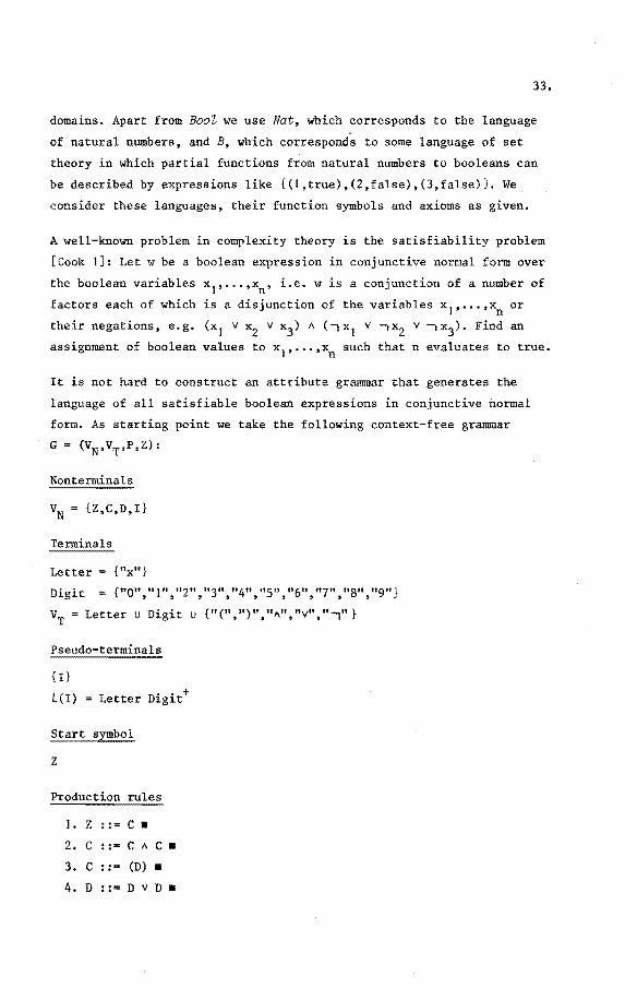
A well-known problem in complexity theory is the satisfiability problem
(Cook 1]: Let w be a boolean expression in conjunctive normal form over
the boolean variables x 1, ••• ,xn' i.e.wis a conjunction of a number of
factors each of which is a disjunction of the variables x 1, ••• ,xn or
their negations, e.g. (x1
v x2 v x3
} A (-,x1
v ..,x2
v 1x3). Findan
assignment of boolean values to x1
, ••• ,xn such that n evaluates to true.
It is not hard to construct an attribute grammar that generates the
language of all satisfiable boolean expressions in conjunctive normal
form. As starting point we take the following context-free grammar
G = (VN,VT,P,Z):
VN = {Z,C,D,I}
Terminals
{"x"} Letter
Digit {"0","1","2","3","4","5","6","7","8","9"}
VT =Letter U Digit u {"(",")","A","v","ï"}
{I}
L(I) = Letter Digit+
Start symbol
z
I. z : := c. 2. c : := c A c. 3. c ::= (D) • 4. D : := D V D •
34.
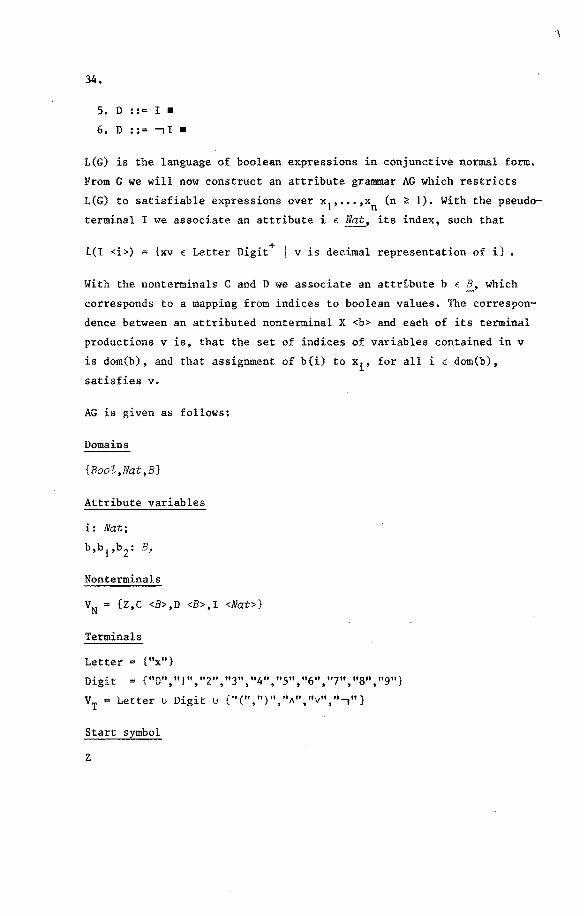
5. D : := I •
6. D ::= ïl •
L(G) is the language of boolean expressions in conjunctive normal form.
From G we will now construct an attribute grammar AG which rastricts
L(G) to satisfiable expressions over x 1, ... ,xn (n ~I), With the pseudo
terminal I we associate an attribute i E Nat, its index, such that
L(I <i>) = {xv E Letter Digit+ I v is decimal representation of i}.
With the nonterminals C and D we associate an attrtbute b E which
corresponds to a mapping from indices to boolean values. The correspon
dence between an attributed nonterminal X <b> and each of its terminal
productions v is, that the set of indices of variables contained in v
is dom(b), and that assignment of b(i) to x., for all iE dom(b), l.
satisfies v.
AG is given as follows:
Domains
{Bool,Nat,B}
Attribute variables
i: Nat;
b,b 1,b2: B,
Nonterminals
VN = {Z,C <B>,D <B>,I <Nat>}
Terminals
Letter
Digit
{"x"}
{"0","1","2","3","4","5","6","7","8","9"}
VT =Letter u Digit u {"(",")","A","v","ï"}
Start symbol
z
\

35.
Pseudo-terminals
{I <Nat>}
For all i E Nat:
L(I <i>) = {xv E Letter Digit+ I v is decimal representation of i} .
Grammar rules
I. Z : := C <B> •
(! n: Nat n > 0 dom(b) {l, ... ,n})
2. c <b> : := c <b> 1\ c <b> •
3. c <b> : :: (D <b>) • 4. D <b> : := D <b 1> V D <b2> •
dom(b 1) n dom(b2) lP
dom(b 1) u dom(b2) dom(b)
b/dom(b 1) = b 1 ~ b/dom(b2) bz
s. D <b> : := I <i> •
b {(i,true)}
6. D <b> : := .,I <i> •
b = {(i,false)}
The picture on page 36 corresponds to an attributed derivation tree t:
FAD(t,(x1
v x2 v x3
) A (-,x1 v -,x2 v -,x3)). We can see from this tree
that the expression (x 1 v x2 v x3
) A (-, x1 v -, x2 v ..., x3) is satisfied
by the assignment x 1,x2 ,x3 := true,false,false.
Several important observations can be made with respect to this example.
The first observation is that the attribute grammar is ambiguous, i.e.
there exist other attributed derivation trees for the same expression.
E.g. the node marked with * might equally well be labelled with either
of the attributed nonterminals D <{(2,f),(3,t)}> or D <{(2,t),(3,f)}>.
This ambiguity is a consequence of the fact that the rule condition of
grammar rule 4 can be satisfied in several ways that lead to identical
terminal strings. In fact there exist even more attributed derivation
trees for the same expression, due to the ambiguity of the context-free
grammar G.

z
I C<{(l,t),(2,f),(3,f)}> ------r--
C<{(l,t),(2,f),(3,f)}>
D<{(l,t),(2,f),(3,f)}> D <{ (I, t), (2, f), (3, f)} >
* D<{(l,t)}> D<{(2,t),(3,t)}> D<{(I,f)}> D <{ (2,f), (3,f) }>
D<{(2,f)}> D<{(3,f)}>
r Î1<2> Î1<3>
D<{(2,t)}> D<{ (3,t) }>
r I I <I> I <2> I <3>
I XI V x2 V x3 A V V
{For comrnent on the node marked with a "*" see page 35}
{"true" and "false" have been abbreviated to "t" and "f" respectively}

37.
The secoud observation concerns the complexity of the parsing problem
for this example. Since L(AG) is the set of all satisfiable boolean
expressions it follows that satisfiability of a string w can be deter
mined by ~n attempt to construct at: FAD(t,w). Since the satisfiabil
ity problem is NP-complete it fellows that for this example the
parsing problem is NP-complete.
2.2.4 Implementation concerns
Definitions 2.12-2.21 and theorem 2.22 have been presented in a way
closely resembling definitions 2.1-2.6 and theerem 2.7 in order to
stress the analogies and differences with context-free grammars.
Definitions 2.12-2.18 embody a generative interpretation of attribute
grammars, whereas theerem 2.22.2 justifies the accepting interpretation
that a string w belengs to L(AG) fif a t: FAD(t,w) can be constructed
for it. Here we will concern ourselves with additional aspects that
make such a construction practically feasible and that relate our view
of attribute grammars to the more traditional view.
Let us first present some definitions that enable us to relate the
parsing problem for attribute grammars to that for context-free
grammars. All these definitions are relative to an attribute grammar
AG= (VN,VT,Z,A,sv,R).
Definition 2.23 {bs, base symbol}
bs E (ANF u AN u VT) + (VN u VT) such that
for all (v,~) E (ANF u AN): bs ((v ,~))
for all V E VT: bs(v) = v.
0
Definition 2.24 {br, base rule}
* br E R + VN x (VN u VT) such that
for all r = ((u0 ,<u 1, ••• ,uk>),rc) ER:
0
=V

38.
Definition 2.25 {base grammar}
The base grammar of AG is the 4-tuple (VN,VT,R',Z), where
R' = {br(r) I r E R}.
0
Definition 2.26 {bt, base tree}
Let ADT be the set of all attributed derivation trees of AG. Let DT be
the set of all derivation trees of the base grammar of AG.
bt E ADT + DT such that
for all v E VT: bs(v) = v
D
The definitions above suggest a way to attack the parsing problem for
attribute grammars. Let AG be an attribute grammar and let G be its
base grammar. In order to construct a t: FAD(t,w) for a string w E VT'
first construct at': FD(t',w). Second,; augment the nodesof t' with
attributes in such a way that the rule conditions of the corresponding
grammar rules are satisfied. If this process succeeds the result is a
t: FAD(t,w) and bt(t) = t'.
The complexity of the attribution process can be reduced by imposing a
partial order on attribute evaluations as follows: Each attribute
position of an attributed nonterminal is classified as either inherited
or synthesized. In the presentation of the attribute grammar this can
be indicated by a '-' or '+' respectively. A rule form which first
appeared as
then appears as
::= V1<-i
1,+s
1> ••• V <-i ,+s > • - - n -n -n
where for each j: 0 :<: j S: n the couple i.,s. is a "partition" of x •• -J -J -J
The corresponding rule condition P(~o····•!n) can be transformed to an
evaluation rule by writing it as:
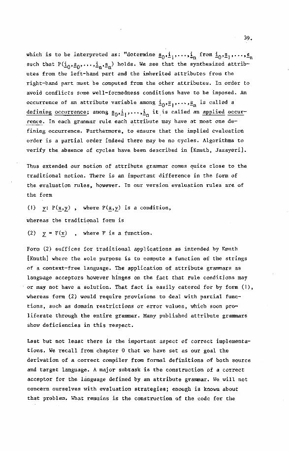
39.
which is to he interpreted as: "determine s0,i 1, ••• ,i from i 0 ,s 1, ••• ,s - - -n - - -n such that P(i0 ,~0 , ••• ,in'~n) holds. We see that the synthesized attrib-
utes from the left-hand part and the inherited attributes from the
right-hand part must he computed from the other attributes. In order to
avoid conflicts some well-formedness conditions have to be imposed. An
occurrence of an attribute variabie among io•~ I' ... '~n is called a
~~==~ occurrence; among !o•it••··•in it is called an applied occur
rence. In each grammar rule each attribute may have at most one de
fining occurrence. Furthermore, to ensure that the implied evaluation
order is a partial order indeed there may be no cycles. Algorithms to
verify the absence of cycles have been described in [Knuth, Jazayeri].
Thus extended our notion of attribute grammar comes quite close to the
traditional notion. There is an important difference in the form of
the evaluation rules, however. In our version evaluation rules are of
the form
(1) z: P(~,z) , where P(~,z) is a condition,
whereas the traditional form is
where F is a function.
Form (2) suffices for traditional applications as intended by Knuth
[Knuth] where the sole purpose is to compute a function of the strings
of a context-free language. The application of attribute grammars as
language acceptars however binges on the fact that rule conditions may
or may nothave a solution. That fact is easily catered for by form (l),
whereas form (2) would require provisions to deal with partial func
tions, such as domain restrictions or error values, which soon pro
liferate through the entire grammar. Many publisbed attribute grammars
show deficiencies in this respect,
Last but not least there is the important aspect of correct implementa
tions. We reeall from chapter 0 that we have set as our goal the
derivation of a correct compiler from formal definitions of both souree
and target language. A major subtask is the construction of a correct
acceptor for the language defined by an attribute grammar. We will not
concern ourselves with evaluation strategies; enough is known about
that problem. What remains is the construction of the code for the

40.
individual attribute evaluations, a significant part of the total
compiler code. Our version of attribute grammars supports this task in
two respects:
the rule conditions of the grammar rules may be used directly as
post-conditions for the code to be constructed;
since attribute structures correspond to algebraic specifications
of abstract data types all of the programming methodology avail
able in that field can be applied directly to the implementation
of attribute domains and their associated operations.
Here we will not elaborate on these as,pects. They will be treated
extensively in a subsequent report [Hemerik].
Above we have described how by additidn of "implementation aspects"
from our version of attribute grammar an attribute grammar in the
traditional sense may be obtained. These aspects have often unneces
sarily influenced and complicated language specifications. We hope to
have made clear that they can, and should, be separated from language
definition aspects.
2.3. Formal syntax of the kemel language
In this sectien we will develop the formal syntax of the kemel
language. In sectien 2.3.1 we present as first approximation a context
tree grammar. In section 2.3.2 this grammar is extended to an attribute
grammar that captures all context dependent properties as well.
2.3.1. A context-free grammar for the kernel languages
The kemel language is much like the language fragment contained in
[Dijkstra 2]. Roughly speaking it consistsof the following ingredients:
the statements abort, skip, multiple assignment, alternative
statement, repetitive statement, bleek;
integer and boolean expressions;
explicit deelaratien of variables.

With the exception of blocks and declarations the constructs have the
same appearance as in [Dijkstra 2]. Variable declarations are similar
to those in Pascal. The rest of the grammar should speak for itself.
Nonterminals
VN = {Prog,Block,Decs,Stat,Type,Ids,Id,Vars,Var,Exprs,Expr,Gcs,
Dop,Hp,Con}
Terminals
Letter {"a", ••• ,"z"}
Digit {"0", ••• ,"9"}
Opl {"+", "-", "-."}
Op2 {"*","+","-","=",":f","<",":$:",">",";;:::","A","v","=>","~"}
Typesym {"int","bool"}
Consym {"true","false"}
Statsym {"skip","abort"}
Sym {"I[","] l","l",",",":",";", "0","+",":=","(",")",
"if","fi","do","Od","var"}
VT Letter u Digit u Op! u Op2 u Typesym u Consym u Statsym u Sym.
Start symbol
Prog
Pseudo terminals
{Id,Dop,Hop,Con,Type}
L(Id) = Letter(Letter u Digit)* \ (Typesym u Consym u Statsym)
L(Dop)
L(Hop)
L(Con)
Op2
Op! .. + D1.gl.t u Consym
L(Type) = Typesym
41.
42.
\
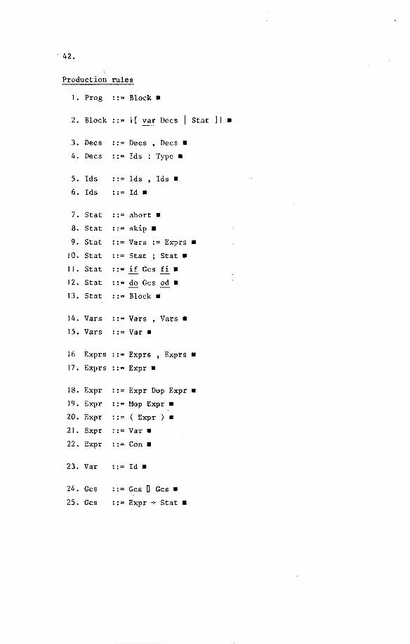
Production rul es
I. Prog .. Block •
2. Block : := I [ var Decs Stat l I • 3. Decs ::= De es • Decs • 4. Decs ::= Ids Type •
s. Ids : := Ids • Ids • 6. Ids : := Id •
7. Stat ::= abort • 8. Stat ::= skip •
9. Stat : := V ars := Exprs • 10. Stat : != Stat Stat • IJ. Stat : := if Gcs fi•
12. Stat : := do Gcs od •
13. Stat : := Block •
14. V ars : := V ars '
V ars • IS. V ars .. Var •
16 Exprs : := Exprs ' Exprs •
17. Exprs ::= Expr •
18. Expr .. Expr Dop Expr •
19. Expr ::= Uop Expr •
20. Expr : : == ( Expr ) • 21. Expr ::= Var •
22. Expr ::= Con •
23. Var : := Id •
24. Gcs : := Gcs 0 Gcs •
25. Gcs : := Expr + Stat •

2.3.2. An attribute grammar for the kernel language
Upon the·language defined insection 2.3.1 a number of context condi
tions are imposed in order to exclude programs like the following:
I[ var x: int I I[ var x bool, i : int, i,b bool I
x,z : 3,4; do true > (3 A4 * b) 7 b, b :~ 3 od
]I;
b := x > 3
1 I
Informally stated the context conditions are as follows:
Within a declaration part of a block each variabie may occur at
most once.
Each variabie occurring in a statement must be declared in some
surrounding block.
Redeclaration of variables in nested blocks is allowed. This
point will be reconsidered in chapter 4.
Expressions should be well-formed with respect to priorities of
operators and types of operands.
43.
Left part and right part of assignments should be of corresponding
lengtbs and types.
Within the left part of an assignment each variabie may occur at
most once.
For the formal rendering of the above we will introduce a number of
domains and operations. Below we provide some informal explanation con
cerning their purpose. This explanation may help in reading the language
specification but is not part of it.
Bool, Int:
Need no further explanation.
Pvio:
Used to indicate the priorities of operators and expressions. The
elements of Pvio are those of Int corresponding to the numbers 1, ••• ,7.

44.
Type:
Used to indicate the type of expressions and variables. We take
Tyr;e = Typesym.
Name:
Used to distinguish between various identifiers. We take
* Name = Letter(Letter u Digit) •
Names:
Used to indicate the colleetien of narnes occurring in a deelaratien
part or in the left part of an assigrunent. An expression ns E Narnes
either of the ferm [n]N' where n E f!ame, or of the ferm ns 1 ~ ns2,
where {ns1 ,ns
2} ~ Names. ns may be thought of as a bag of narnes, in
is
which case the ether operations ~ and #N correspond to memhership
and number of occurrences respectively. From the axioms it is easy to
prove that (n inN ns) = (#N(n,ns) ~ 1).
Types:
Used to indicate the sequence of types corresponding to the left part
or right part of an assignment. An expression ts E Types is either a
singleton of the ferm [t]T, where t E Type, or of the ferm ts 1 ~T ts 2,
where {ts 1,ts2 } ~Types. To compensate for the ambiguities in de pro
duction rules for Vars en Exprs there is an axiom which states
associativity of ~T.
Decs:
Used to record the essential information of a deelaratien part, viz. a
colleetien of (name,type) associations. An expression d E Decs is
either of the ferm [ns,t]D' where ns E Narnes and t E Type, or of the
ferm d 1 \EY d2, where {d 1,d2} ~ Decs. d may be thought of as a bag of
pairs (name,type), in which case the eperation inD corresponds to
memhership and the operatien #D to number of occurrences of a name.
Env:
Used to record the environment of a construct, i.e. the essential
information of all declarations occurring in bleeks surrounding the
construct, taking into account the nesting of bleeks. An expression
e E Env is either Empty, \vhich corresponds to an empty colleetien of

declarations, or of the form Ext(e,d), where e € Env and d €
which corresponds to an ordered extension of an environment with a
colleetien of declarations.
45.
After this informal presentation reading of the grammar should pose no
serious problems. The presentation follows.
Domains
{BooZ,Int,Name,JYpe,Prio,Names,Types,Deas,Env}
Attribute variables
n,n1 ,n2: Name;
t,t0,t 1,t2
: Type;
p,pO,pl,p2: Prio; ns,ns
0,ns
1,ns2: Names;
ts,ts0,ts
1,ts2: Types;
d,d0,d 1,d2: Deas;
~.e0 ,e 1 : Env.
on Prio
Frio {e € Int I the integer value corresponding to e is an element
of { 1, ••• , 7} } •
= Typesym.
Operatiens on Name
Name = Letter(Letter u Digit)*.
Operatiens on Names
[.] N
Name + Names
. \!I . Names * Names + Names
. ~. Name * Narnes + BooZ 11 N( • '•) Name * Narnes + Int
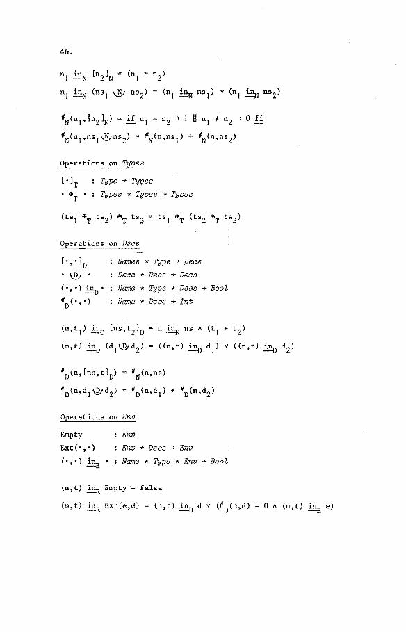
46.
n 1 ~ [n2 ]N = (n 1 ~ n2)
n1 ~ (ns 1 ~ ns 2) ~ (n1 ~ ns 1) v (n1 ~ ns2)
Operatiens on Types
[•]T Type +Types • <&
T Types * Types + Types
Operatiens on Deas
[ •' • ]D Names * Type + Deas . IJV . De as * Deas + Deas
(.'.) i~. Name * Type * Deas + BooZ # D ( •' •) Name * Deca + Int
#N(n,ns) #0
(n, [ns, t]0
)
#D(n,dl @d2) #D(n,dl) + #D(n,d2)
Operatiens on Env
Empty
Ext(•,•)
(n, t)
(n, t)
Env
Env * Deas + Env
Name * Type * Env + Boot
Empty ·= false
Ext(e,d) = (n,t) in0 d v (#0 (n,d) 0 A (n,t) ~ e)

47.
Nonterminals
VN = {Prog,Block <Env>,Decs <Dees>,Stat <Env>,Type <Type>,Ids <Names>,
Id <Name>,Vars <Env,Names,Types>,Var <Env,Name,Type>,
Exprs <Env,Types>,Expr <Env,Prio,Type>,Gcs <Env>,
Dop <PY.io, ,Type,Type>,Mop <Type,Type>,Con <Type>}.
Terminals
Letter {"a", ••. , "z"}
Digit {"0", ••• ,"9"}.
Opl {"+","-","-,"}
Op2 {"*", "+","-","=u.,"/","<", n~u, ">",";::::'*,u A", "v", "=*u, nf:!:!'ln}
Typesym {"int","bool"}
Consym {"true","false"}
Statsym = {"skip", "abort' .. }
Sym {'' 1 [tt, '']I", trI'' ,n, 11, ••:n, ";", "0'', ''-+'', '':='', ''(", '')'';
"if","fi","do","od","var"}
VT Letter u Digit u Opl u Op2 u Typesym u Consym u Statsym u Sym.
Start symbol
Prog.
Pseudo terminals
{Id <Name> ,Dop <Prio,Type ,Type ,Type>,Mop <Type ,Type>,Con <T::rpe>,
Type <Type>}.
For all n E Name:
L(Id <n>) = {n} \ (Typesym u Consym u Statsym)
L(Dop <l,bool,bool,bool>) {' ... ". "*"}
L(Dop <2,bool,bool,bool>) {"v"}
L(Dop <3,bool,bool,bool>) {"A"}
L(Dop <4,bool,int,int>) {"=",":J:.","<n,n::s;n,n>n,n~tt}
L(Dop <S,int,int,int>) = {"+","-"}
L(Dop <6,int,int,int>) {"*"}

48.
L(Mop <int, int>) {"+","-"}
L(Mop <bool,bool>) {"•"}
L(Con <int>) Digit +
L(Con <bool>) Consym
L(Type <int>) = {"int"}
L(Type <bool>) {"bool"}
I. Prog ::::::::: Block <e> • e = Empty
2. Block <eo> : := I [ var Decs <d> I Stat <el> 1 I • (A n: Name I #
0 (n,d) ::;; I)
el = Ext(e0 ,d)
3. Decs <do> . . Decs <dl> ' De es <dz> •
do = dl 0V d2
4. De es <d> : ::;::; Ids <ns> : Type <t> • d = [ns,t]D
s. Ids <ns0
> : := Ids <ns 1> '
Ids <ns2> •
nso = ns 1 \IV ns2
6. Ids <ns> ::; Id <n> •
ns = [n]N
7. Stat <e> : := abort •
8. Stat <e> : := skip •
9. Stat <e> : := V ars <e,ns,ts> := Exprs <e,ts> • (A n: Name I # N(n,ns) ::;; I)
JO. Stat <e> ::= Stat <e> ; Stat <e> •
11. Stat <e> : := if Gcs <e> fi•
12. Stat <e> ::=do Gcs <e> od •

49.
13. Stat <e> : :"' Block <e> •
14. Vars <e,ns0,ts0> ::"' Vars <e,ns 1,ts 1> Vars <e,ns2 ,ts2> •
ns0
ns1 ~ ns 2
15. Vars <e,ns,ts>
17. Exprs <e,ts>
21. Expr <e,p,t>
22. Expr <e,p,t>
23. Var <e,n,t>
24. Gcs <e>
25. Gcs <e>
ts0 ts 1 eT ts2
: := Var <e,n, t > • ns = [n]N
ts [t ]T
::= Exprs <e,ts1>
' ts0 = ts
1 @T ts2
::= Expr <e,p,t> •
ts = [t]T
Exprs <e,ts2> •
::= Expr <e,p 1,t 1> Dop <p
0,t
0,t
1,t
2> Expr <e,p
2,t2> •
Po 5o pI
Po < Pz
: :=
::= ( Expr <e,p 1,t>) •
Po = 7
::=Var <e,n,t> •
p "' 7
::=Con <t> •
p "' 7
: := Id <n> •
(n,t) in e --€:
Gcs <e> D Gcs <e> •
::= Expr <e,p,t> +Stat <e> •
b = bool

50.
CHAPTER 3
PREDICATE TRANSFORMER SEMANTICS FOR THE KERNEL LANGUAGE
3.0. Introduetion
In [Dijkstra I, Dijkstra 2] it has been proposed to define the seman
tica of programming languages by means of so-called predicate trans
farmers. The idea is that a set of states of a computation can be
characterized by a predicate in terros of the program variables and
that all relevant aspects of a statement are captured by its predicate
transformer, a function from predicates to predicates. Two kinds of
predicate transfermers are discussed, viz. the "weakest pre-condition"
wp and, to a lesser extent, the "weakest liberal pre-condition" wlp.
For a certain mechanism S and a post-condition R the corresponding
weakest pre-condition wp(S,R) is defined as follows (we quote from
[Dijkstra 2]):
"The condition that characterizes the set of all initial states
such that activatien will certainly result in a properly termi
nating happening leaving the system in a final state satisfying
a given post-condition is called 'the weakest pre-condition
corresponding to that post-condition'.".
Experience bas shown that predicate transfermers are a suitable vehicle
for discussing issues of program correctness. Hhen dealing with ques
tions of semantica or implementation correctness further elaboration is
required, however. Let us mention a few problems:
As remarked by [Plotkin) the definition quoted above "is admirably
clear and perfectly precise once we know what conditions and
mechanism~ are". In [Dijkstra 2] several mechanisms (statements)
are defined but no definition of conditions is given. The result
is that of the central concept of the language definition, the
predicate transformer, two important aspects, its domain and its
range, are left undefined. That such an omission may lead to
complications can be illustrated as follows.
51.
Let C be a set of conditions that serves as domain and range of
predicate transformers. Two statements s1 and s2 may be considered
equivalent fif for all Q E C: wp(S 1,Q) = wp(s2,Q).
In the extreme case that C = ~ it follows that all statements
are equivalent.
In [Dijkstra 2] the predicate transfarmers of the statements
skip and x := E are defined by wp(skip,R) = R and
wp(x := E,R) = ~~· respectively. In case that C contains
no conditions that depend on x these statements are equiva
lent, otherwise they are not.
Simple and artificial as these examples may seem, they suffice to
show that the degree to which statements can be distinguished
depends on the "richness" of the set of conditions C, which
therefore is an essential component of a language definition.
Another point of concern is the nature of conditions. In I
[Dijkstra 2] the distinction between formal expressions and the
objects they denote is simply done away with as a "mannerism".
We just cannot afford such an attitude in language translation:
the very existence of the notion of translation is based on the
fact that different formal expressions may denote the same object.
In the literature on predicate transformer semantics we find both
an intensional point of view, where conditions are considered as
elements of a formal language [Back 2, de Bakker, t1ilne], and an
extensional point of view, where conditions are identified with
the sets of states they characterize [Plotkin, Wand]. Both ap
proaches are feasible, but each has its specific problems and
there are marked differences, e.g. with regard to the lattice
theoretical framework required to deal with recursively defined
conditions.
The last remark above hints at a different problem. The definition
of wp(DO,R) in [Dijkstra 2] essentially employs a fixed point
approximation, although this is not stated explicitly. Since in
further development of predicate transformer semantics we will not
only encounter recursively defined predicates but also various
kinds of recursively defined predicate transformers it seems wise

52.
to employ a general theory to deal with recursive definitions,
such as Scott's lattice theory [Scott 2].
A final point concerns the expressibility of conditions. In
general, the pre-condition of a statement will depend on the
variables and expressions occurring in that statement and the
language of conditions should be rich enough to express these
dependencies. A good candidate for a condition language seems to
be the set of first order predicates in terms of the variables and
operations of a program. Yet it appears that this language is not
sufficiently powerful to express pre-conditions of repetitions.
[Back I] gives a simple counter-example. Either a largersetof
operations should be employed (which raises the problem of deter
mining whether the condition language is closedunder that set),
or a more powerful logic should be employed such as the infinitary
logic L (Back l, Karp, Scott 1]. [Back l] shows that this logic WJW
is sufficiently powerful to express the weakest pre-conditions for
the language of [Dijkstra 2].
It is the purpose of this chapter to provide a firm foundation for
predicate transformer semantics by presenting additional definitions
and by making the connections with other branches of matbematics such
as lattice theory and more explicit. In doing so we will also
pave the way for the development of a predicate transformer semantics
for language constructs ether than statements in chapters 4 and 5.
The first important decision we take in this respect is to adopt an
intensional view of conditions, i.e. to consider them as elements of a
formal language. The grammatica! tools developed in chapter 2 enable us
to define very precisely the condition language to be used with a set
of statements, in particular as regards the contextual properties.
These properties play an important role in chapter 4, where constructs
involving changes of context are considered, such as blocks and proce
dures. The close connections between programming language and condition
language also make it easier to study Hoare-like correctness formulae
and proof rules, as statements and the conditions associated with them
can be considered at the same language level, and transitions between
syntactic and semantic domains can be kept to a.minimum.
53.
Imposing a suitable lattice structure on the condition language
requires some provisions. On the one hand we will introduce infinitary
formulae and proof rules as in L00100 • On the other hand we will develop
some theory for a special kind of lattices which we call countably
complete lattices and which provide the desired structure to deal with
recursive functions of conditions. This chapter therefore has the
following structure. Insection 3.1 we collect both old and new results
from lattice theory that will frequently be used in the current and
following chapters. In section 3.2 we first define a condition language
and subsequently study the predicate transfermers wp and wlp in a
lattice-theoretical framework. In section 3.3 we use these definitions
to develop logies in the of [Hoare 2] for proving partial and
total correctness of programs.
No te
Thus far we have used the term "predicate transformer" introduced by
Dijkstra. Because the notion of condition differs considerably from the
notion of predicate as used in logic, we will henceforth use the term
"condition transformer".
0

54.
3.1. Some lattice theory
In this section we collect some results concerning complete partially
ordered sets, (countably) complete lattices, continuous functions,
fixed points, etc. These results form the basis for the study of condi
tion transfarmer semantics in subsequent sections. Part of the material
presented here is well-known and has mainly been included for complete
ness's sake. Lemmas and theorems that appear without proof have been
taken over literally or with slight adaptations from [de Bakker), as
have some definitions. Less-known and new results appear with full
proofs. The proofs of some subsidiary results have been delegated to
Appendix A.
3.1. I. General definitions
The central notions of our summary are those of a complete partially
ordered set (cpo) and of a countably-complete lattice (cel). Since both
of them are special forms of partially ordered sets we begin our
sequence of definitions with that of the latter notion.
;;;;..;;..=;;;.;;:.;:.=:..::.....=3..:.. • ..:..1 {partially ordered set}
A partially ordered set is a pair (C,!;.), where Cis an arbitrary set
and ~ is a binary relation on C satisfying
No te
(A x E C x ~ x)
(~ x,y E C (x ~ y A y ~ x) ~ x = y)
(~ x,y,z E C I (x ~ y A y ~ z) ~ x ~ z)
{reflexivity}
{antisymmetry}
{transivity}
Occasionally we will also use the relations c and ~. given by
(~ x,y E C I x·C y ~x~ y A x I y) and (~ x,y E C I x 2 y ~ y ~x),
respectively.
0
A subset of a partially ordered set may have a greatest lower bound or
a least upper bound:

-=-=-===-=-==-'3...:.'...:.2 { gl b , 1 ub }
Let (C,~) be a partially ordered set, and let X ~ C.
I. y € Cis called the greatest lower bound (glb) of X if
(A X E X y !;': x)
(!!; Z E C (!!;; x E X z t:;. x) '* z !:: y)
The glb of a set X will be denoted by nx.
2. y E C is called the least upper bound (lub) of X if
(!!; X E x x Ë y)
<!! z E C (!! X E x x !:: z) '* y !: z)
The lub of a set X will be denoted by u x. 00
3. The glb and lub of a sequence <x0
,x1
, ••• > are denoted by F=o x. l
00
and i~O xi' respectively.
0
No te
From the definitions above it follows that if for X
exist, they must be unique.
c nx or ux
0
Definition 3.3 {chain}
Let (C,t:;_) be a partially ordered set.
Cl
I. An ascending chain in (C,!:) is a sequence <x0,x1
, ••• > such that
(!!;;i I i~ 0 I xi ~ xi+l).
2. A deseending chain in (C,t:;_) is a sequence <x0 ,x1
, ••• > such that
(A i I i ~ 0 I x. 'J x. I). - l.- J.+
55.
We will primarily be interested in a special kind of partially ordered
sets, viz. countably-complete lattices. lt will be useful to relate
that notion to some better-known notions, however. Hence the following
definitions.

56.
Definition 3.4 {cpo}
A complete partially ordered set (cpo) is a partially ordered set (C,~)
such that
the glb of C exists,
each ascending chain <x0 ,x1, ••• > bas a lub i~O xi.
0
Definition 3.5 {uccl, deel}
(uccl) is a partially ordered
set (C,~) with the property that each countabl·e subset has a lub
and each finite subset bas a glb.
IJ
2. A downward countably-complete lattice (deel) is a partially
ordered set (C,~) with the property that each countable subset has
a glb and each finite subset has a lub.
Definition 3.6 {cel}
A countably-complete lattice (cel) is a partially ordered set (C,~)
with the property that each countable subset has both a lub and a glb.
IJ
Definition 3.7 {cl}
A complete (cl) is a partially ordered set (C,~) with the
property that each subset bas both a lub and a glb.
0
No te
In definition 3.7 it would suffice to require that each subset X C
bas a lub. It can easily be shown that in that case it also has a glb,
viz. u { y E C (~ x E X I y ç_ x)}.
0
Lemma 3.8
Let (C,~) be a uccl.
D
I. C has a glb, viz. uÇL
2. C has a lub, viz. n0.

Proof
D
I. ~ is a countable subset of C, hence by definition 3.2.2:
(!!: X E ~
uQI !: z)
x g z) =~> u0!;. z), i.e.
{a}
Let w E C be such that (!!: z E C I w ~ z). Then in particular:
w !; u 0 {b}
From a, b and definition 3.2.1 it fellows that nc = u~.
2. 0 is a finite subset of C. The remainder of the proof is a dual
version of I.
From definitions 3.4-3.7 and lemma 3.8 it fellows immediately that
every cl is a cel;
every cel is both a uccl and a deel;
every uccl is a cpo;
the dual of a cl is a cl;
the dual of a cel is a cel;
the dual of a uccl is a deel.
57.
In the sequel we will frequently make use of these relations; e.g. if
we have proven a property of cpo's we will use the fact that it also
holds for uccl's and that the dual property holds for dccl's.
No te
If (C,!;.) is a cpo (uccl, deel, cel, cl) its glb n C will be written as
1 {pronounced as "bottom"}. If (C,!;.) is a uccl (deel, cel, cl) its
lub u C will be written as T {pronounced as "top"}.
D
Our interest will focus on functions on lattices of the kinds just
introduced. An important property of certain classes of these functions
is that under a suitably defined order they also have a lattice struc
ture. That order is defined by

58.
Definition 3.9 {standard order on functions}
Let c1 be a set and (C2 ,~) be a partially ordered set. The standard
order ~ on cl + c2 is defined by:
(! f. g E c I + c2 I f !;. g * (! x E c I I f (x) t;.2 g (x)) •
D
It can easily be verified that the standard order is a partial order
indeed.
Theorem 3. I 0
Let c 1 be a set and (c2,t;.) be a partially ordered set. Let ~ be the
standard order on cl + c2.
I. If (c2
,t;.2 ) is a cpo, then
(c 1 +C2 ,~) is a cpo.
- ie +C = (Àx I ie ). · I 2 2
for each ascending chain <fi>:=O in c1 + c2 :
00
i~O fi (Àx I
(C 1 +C2 ,~) is a uccl.
for each countable F s c1 -+ c2 : UF
for each finite
0
Corollary 3. 11
If c1 is a set and (c2 .~2 ) is a uccl:
0
I. See [de Bakker].
(ÀX fiF f (x))
(ÀX ilF f(x))

D
2. I. Let F be a countable subset of c1 + c2• From the fact that
(C2 ,~2) is a uccl it follows that for all x E c1:
f~F f (x) E c2 •
Let g = (h I u f(x)). We show that g = UF, fEF
=t (! f E F I (! x E C 1 I f (x) ~2 f~F f (x)))
=t {definition 3.9, definition of g}
(! f E F I f ~ g)
(A f E F I f ~ h)
=t {definition 3.9}
(!:_ f E F I (!:_x € cl I f(x) [;_2 h(x))
{interchange quantifiers}
<!x E cl I (! f E F I f(x) ~2 h(x)))
• {definition lub in c2}
f(x) ~2 h(x))
{definition
(!x E cl I g(x) ~2 h(x))
{definition 3.9}
g ~ h •
59.
2. The proof that each finite subset of c1 + c2 has a glb is a
dual version of the proof above.

•
60.
3.1.2. Strictness
Definition 3.12 {strictness}
l. Let (c 1 ,~ 1 ) and (C2,s
2) be cpo's (uccl's, dccl's, ccl's, cl's),
and let f E c1 ~ c
2•
f is called ~-strict if f(~c 1 ) = ~c2 •
2. Let (c 1 ,~ 1 ) and (c2 ,~2 ) be uccl's (dccl's, ccl's, cl's), and let
f E c1
... c2
•
f is called T-strict if f(Tc1) Tc
2•
D
For the determination of the strictness of a composite function in
C + C the following theorem may be useful.
Theerem 3.13
Let (C,~) be a cpo.
Let s! = {f E c ... c I f is !-strict}.
I. (\x 1) E s ~
2. (À x x) E S 1
3. for all f,g E S~ fog E S1 ,
If, moreover, (C,S) is a uccl, then
4. for each countable subset F c S (Àx I U f(x)) E s1 - ~ f,;:F
5. for each finite nonempty subset F ~ S1: (Àx f(x)) E: s!
0
Pro of
1,2,3: trivia!.
4. (ÀX u f (x)) (i C 1 ) "' u füc ) u ~c 1c2 fEF fEF I fEF 2
5. (\x I n f(x))(!c ) n f(!c ) n ~c {F nonempty} ~c fEF I f,;:F I fEF 2 2
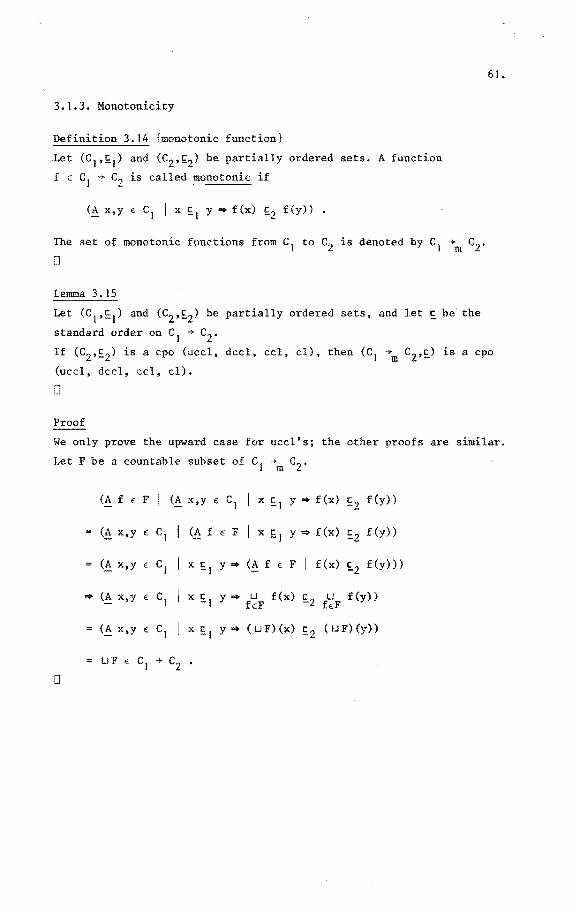
3.1.3. Monotonicity
Definition 3.14 {monotonie function}
Let (c 1 ,~ 1 ) and (c2 ,~2 ) be partially ordered sets. A function
f E c1 + c2 is called monotonic if
(~ x,y " c1 I x ç_1 y .. f(x) s2 f(y))
The set of monotonic functions from c1 to c2 is denoted by c1
+m c2 •
D
Lemma 3.15
Let (c1,s
1) and (C2 ,~2 ) be partially ordered sets, and let s be the
standard order on cl + c2.
61.
If (c2 ,~2 ) is a cpo (uccl, deel, cel, cl), then (c 1 +m c2,s) is a cpo
(ueel, deel, cel, cl).
D
Proof
We only prove the upward case for uccl's; the other proofs are similar.
Let F be a countable subset of c1
+m c2 •
(A f E F x,y E cl x ~1 y .. f(x) E2 f(y))
(~ f E F x~~ y.., f(x) ~ 2 f(y))
x El y • (Af E F I f(x) ~2 f(y)))
.. (~ x,y E cl I x y .. u f(x) s2 u f(y)) fE:F fEP
(~ x,y E cl I x y.., (UF)(x) ~ 2 (UF)(y))
D

62.
3. 1.4. Conjunctivity and disjunctivity
Definition 3.16 {n and u as infix operators}
Let (C,ç;.) be a uccl.
The infix operators n,u: C x C ~ C are defined by:
1. for all x,y E C: xn y = n {x,y} •
2. for all x,y E C: x u y =u {x,y}
D
In terms of these operators we can define the notions conjunctivity and
disjunctivity. In lattice theory these notions are usually called
multiplicativity and additivity, respectively.
Definition 3.17 {conjunctivity, disjunctivity}
Let (c 1 ,~ 1 ) and (c2 .~2 ) be uccl's, and let f E c1 + c2 •
0
if (~ x,y E C]
2. f is called .;;;..;;;."-"'..:.;.;;...;;;..;;;._:_.c:.. if (~ x,y E Cl
Lemma 3.18
f(xn1
y)
f(xu1
y)
Let (c 1 ,~ 1 ) and (c2 ,~2 ) be uccl's, and let f E c1 ~ c2•
IJ
I. if fis conjunctive, then fis monotonie;
2. if f is disjunctive, then f is monotonie.
Pro of
Let x,y E c1 such that x ~~ y.
1. f(x) = f(x n 1 y) f(x) f(y) !:.2
f(y)
2. f(y) = f(x u 1 y) = f(x) u 2 f(y) .22 f(x) •
D
f(x) n2
f(y))
f(x) u2
f(y)).

3.1.5. Continuity
Definition 3.19 {continuity}
I. Let (c1,ç
1) and (c2 ,~2 ) be cpo 1 s.
A monotonic function f E c1 ~mc2 is called ~~~~~~~~
for each ascending chain <xi>i=O in c1:
f(.Ü0
x.) ~= ~
f(x.) • ~
if
The set of upward continuous functions in c1 ~ c2 is denoted by
cl ~uc c2.
2. Let (C 1 ,~ 1 ) and (C2 ,~2 ) be dccl 1 s.
A monotonic function f e c1 ~ c
2 is called
for each deseending chain <x.>~ 0
in c1
: ~ ~=
63.
0
The set of downward continuous functions in c1 + c2 is denoted by
cl +de c2.
No te
In definition 3.19.1 it would be sufficient to require that
f(~Ü",0 x~) f(x.), because f(.Ü0 x.) .Ü0 f(x.) follows from ~ ~ ~ ~= ~ ~= ~
the monotonicity of f. A complementary remark applies to definition
3.19.2.
0
No te
Since continuity is a stronger property then monotonicity it follows
that all properties of monotonic functions also hold for continuous
functions. In some of the forthcoming proofs use will be made of this
fact without explicit reference.
0
As preparatien for some important theorems ccincerning continuity we
first present some lemmas.

64.
Lemma 3.20
1. Let (C,~) be a cpo. Let, for iE {0,1, ••• }, jE {0,1, ••• }, x .. be ~J
elements of C. If
(~ i,j,k,1 0 s i $; k A 0 s j s 1 I xij ~ ~1 )
then
00 "' 00 "" 00
i'=!o j'=!o xij j'=!o i'=!o xij = k'=!o ~k •
2. Let (C,~) be a uccl. Let R,S be two countab1e sets. Let, for
i € R, j E S, x .. be elements of C. Then lJ
0
Pro of
I. See [de Bakker].
2. See Appendix A.
0
Lemma 3.21
Let <xi>7=o and <yi>:=O be two ascending ebains in a uccl (C,~).
I. <x. n y.>~ 0 is an ascending chain. ~ ~ ~=
[]
Proof
See Appendix A.
D
Lenuna 3.22
Let (C,b) be a uccl. Let S be a finite set. Let, for i E S,
jE {0,1, ••• }, x .. be elementsof C. If ~J
(~ i,j,k I i E SA 0 S j s k xij Ç xik)
then
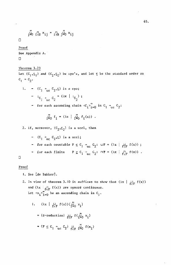
00
j\;!0 i~S xij
D
Pro of
See Appendix A.
D
Theorem 3.23
00
i~S j~O xij
Let (c 1 ,~ 1 ) and (c2
,
cl + cz.
be cpo's, and let c be the standard order on
D
I. (Cl + c2, is a cpo; uc
l.c + cz (Àx I .Lc ) I uc 2
for each ascending chain <f.>~ 0 l. ].=
00
(ÀX I 00
fi(x)} il;;lo f. = il;;lO l.
2. If, moreover, (c2,E2) is a uccl, then
(C 1 +uc c2 ,~) is a uccl;
for each countable F ~ c1
for each finite
+ uc
+ uc
Proof
I. See [de Bakker].
in cl + uc
(ÀX
(ÀX
C2:
fiF f(x))
f:iF f(x))
65.
2. In view of theorem 3.10 it suffices to show that (ÀX I and (Àx I iiF f(x)) are upward continuous.
f(x))
Let <x.>~ 0 be an ascending chain in c1• l. ].=
I. (ÀX I f~F f(x)) x i)
{13-reduction} f(i~O x i)
{F ~ c1 cz} 00
f(x.) + ï'=!o uc l.

66.
"" • {lemma 3.20.2} i~O f~F f(xi)
= {a-expansion} 1.~_""0 (Àx I u f(x})(x.) f"F l
2. The proof that (Àx I n f(x)} is upward continuous is f"F
similar to the one given above, the main difference being
that lemma 3.22 rather than lemma 3.20.2 bas to be applied.
D
For the determination of the continuity of a compesite function in
C ~ C the follewing theerem may be useful:
Theerem 3.24
Let (C,~) be a uccl.
I. For all y E C: (ÀX y) E C ~ c. uc '
2. (Àx I x) E C -+uc C ;
3. fer all f,g E C -+uc C: fog E c ~ c ; uc
4. fer each ceuntable F s c .... C: (ÀX uc
u f(x)) E C ~ fEF uc
c . '
5. fer each finite
0
F c C ~ C: (ÀX n f(x)) E C ~ C • - UC fEF uc
Proef
Let <x.>~ 0 be an ascending chain in c. l. ].=
(ÀX y} (i~O xi) co co
(ÀX I Y;}(xi) I. - y = i'=!o Y i'=!o
2. (ÀX I x)(i~O xi) co "" (ÀX I x) (x.) = i'=!o x. i'=!o ;
l. l.
= .u0
(fog} (x.} l.= l.
4, 5 immediately by theerem 3.23.2 and theerem 3.10.2.
0

67.
ExamEle
Let (C,!;;) be a uccl.
I. For i: ~ i ~ n: let c. l.
E c ;
2. for i: ~ i ~ n: let d. E c ; l.
3. for i: ~ i ~ n: let f. E c .... c l. ue
We show that
(Àx
4. {by I' th. 3.24. 1} for i: ~ i ~ n: (I, x I ei) E c .... c ue
5. {by 4, th. 3. 24.4} (Àx I n ei) c c i';;! I E ....
ue
6. {by 2, th. 3. 24. 1} for i: ~ i ~ n: (À x di) E C + c ; ue
7. {by 3,6, th. 3. 24 .• 4} for i: ~ i ~ n: (ÀX di u fi (x)) E C + c . ' ue
8. {by 7, th. 3.24.5} (À x n
ir:!J (di u fi (x))) E C + c . uc '
3.24.5} n n
(di u 9. {by 5,8, th. (Àx (i';;! I c.) n .n1 fi(x))) E c c .
l. 1.= D
No te
In the sequel we will not give proofs like the one above in detail.
Instead we will simply refer to "repeated application" of theorem 3.24.
D
The following lemma is used in the proof of theerem 3.26.
Lemma 3.25
Let (C,~) be a ueel. Let D = C + C, uc
I. If gE D and <hi>~=O is an aseending ehain in D, then
g 0 (Lill h.) i=O 1

68.
0
Pro of
See Appendix A.
0
Let (C,~C) be a uccl, and let D = C +uc C. With ~D being the standard
order on D we have, by theorem 3.23.2, that (D,~0) is also a uccl. In
the sequel we will often be concerned with functions F E D + D which
will usually be given in the form F (Àf E D I E(f)), where E(f) is an
expression in terms of f, usually in the form (Àx E C I G(f,x)). For
the determination of the continuity of such a function from its com
position the following theorem will be useful.
Theorem 3.26
Let {C,~c) be a uccl, and let D = C +uc C.
I. For all c E C: (H I (Àx I c)) E D + D uc
2. {Àf I (Àx I x)) E D + D uc
3. if (Àf I E1(f)) E D + D and (Àf I E2(f)) E D + D, then uc uc
4. if for all i: s i s n: (H I {ÀX I E.)) E D + D, then ~ uc
(u n I (À x [_gJ E.)) E D + D ;
i= I ~ uc
5. if for all i: :S i :S n: (H I (ÀX I E.)) E D+ D, then ~ uc
(u n Ei)) E I <ÀX I lël D + D •
i=l uc
0

Proof
I.
2.
3.
Letc E C.
C E C
=> {theorem 3.24.1, D = C + uc C}
(Àx I c) E D
• {theorem 3.24.1}
(H I (Àx I c)) E D + D uc
true
=> {theorem 3.24.2}
(Àx I x) E D
=> { theorem 3. 24. 1}
(H I (:\x I x)) E D + D uc
00
Let <fi>i=O be an ascending chain in D.
= {S-reduction}
{for i: I :> i :>: 2: (H j E1• (f)) E D + D}
uc
{lemma 3.25.2}
{13-expansion}
69.

70.
4. (ü I (ÀX I wE.)) i=l l.
{theorem 3.23.2}
(Àf n (ÀX I Ei)) Ll2J
i= I
Üheorem 3.23.2}
n
l~ucDI (H I (ÀX I E.)) • l.
1=1
5. (u I (ÀX 1 m E.)) i=l 1
= {theorem 3.23.2}
(u I rm (ÀX IE.)) i=l 1
{theorem 3.23.2}
n ID~UCDI (H I (Àx I E.)) • 1
i= I 0
3.1.6. Fixed points
Definition 3.27 {fixed point}
Let (C,S) be a cpo, f E C ~ C, x E C
0
I. x is called a fixed point of f if f (x) = x.
2. x is called the least (greatest) fixed point of f if x is a fixed
point of f and, moreover, for each fixed point y of f, x~ y
(x .2 y).
If f has a least (greatest) fixed point it is denoted by ~f (vf).
Theerem 28
I. Let (C,~) be a cpo.
lf a function f E C + C is upward continuous it nas a least fixed

71.
point satisfying
Jlf =
where f 0 = (Àx I x), fi+l fofi for i 2: 0.
2. Let (C,~) be a deel.
If a function f E C + C is downward continuous it has a greatest
fixed point vf satisfying
vf
where f 0 (Àx I x), fi+l
0
Pro of
I. See [de Bakker].
2. By I and duality.
0
fof. for i 2 0. ~
The following simple lemma will be used in several places in combina
tion with the fixed point property y = f(y). Together they form the
basis for the inductive proof rules for repetitions and recursive
procedures.
Lemma 3.29
Let (C,~) be a uccl. Let {xi I i 2 0} s C, y E C. If
<~ i I i 2: o 1 < u x. c y > .. <x. c. y > > O~j<i J - ~ -
then
"' il:!o i: Y •
D
Proof
(~ i I i 2: 0 I ( ~ . x. ~ y) ". (xi !;. y)) 0~]<1 J
{definition lub}
i I i 2: 0 I (~ j I 0 ~ j < i x. !; y) .,. (x. t: y)) J ~ -:
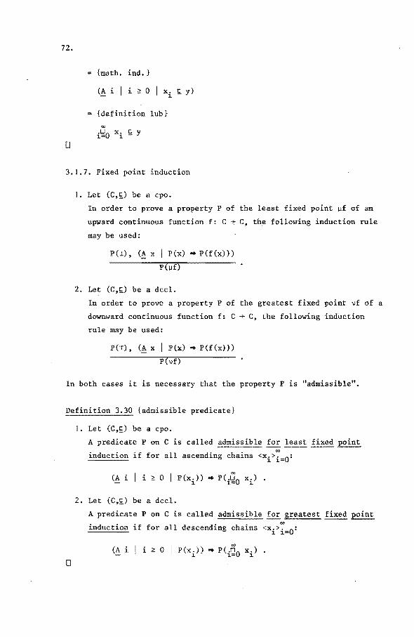
72.
{math. ind.}
<~ i I i ~ o I xi ~ y)
{definition lub}
0
3.1.7. Fixed point induction
1. Let (C,~) be a epo.
In order to prove a property P of the least fixed point ~f of an
upward continuous function f: C + C, the following induction rule
may be used:
P(~), (~x I P(x) • P(f(x)))
2. Let (C,~) be a deel.
In order to prove a property P of the greatest fixed point vf of a
do~rnward eontinuous funetion f: C + C, the following induction
rule may be used:
P(T), (A x P(x) • P(f(x)))
P(vf)
In both cases it is necessary that the propertyP is "admissible".
Definition 3.30 {admissible predieate}
0
1. Let (C,~) be a epo.
A predieate P on C is called admissible for least fixed
induetion if for all aseending ehains <x.>~ 0 : 1 1=
(A i I i ~ 0 I P(x.)) • P(.u0 x.) . - 1 1= 1
2. Let (C,~) be a deel.
A predicate P on C is called admissible greatest fixed point 00
induetion if for all deseending ebains <xi>i=O:
(_A i I i ~ 0 I P(x.)) .. P(.no x.) 1 1= 1

The fixed point induction rule can easily be extended to systems of
functions:
73.
Let, for n ~ l, (C1,!;.1), ••• ,(Cn'~) be ccl's, and let C c1 x ••• x Cn.
On C we define the ordering ~ by:
* (!:_ i I I ~ i ~ n x. l,.
It can easily be verified that (C,~) is also a cel.
Let k: 0 ~ k ~ n.
Let for i: ~i ~ k: fi E C +uc Ci.
Let for i: k+l ~ i $ n: fi E C +de Ci'
In order to prove a property of the least fixed points vf 1, ••• ,vfk and
the greatest fixed points vfk+J'''''vfn the following induction rule
may be used:
P((ll '''' 'l.k' Tk+l '''' 'Tn))'
<!:.x E c 1 P(x) • P((f 1(x), •.. ,fn(i))))
P((vf 1, ••• ,vfk,vfk+J'''''vfn))
We will refer to this version of fixed point induction as simultaneous
fixed point induction
The notion of admissibility has to be extended accordingly: P is
admissible for simultaneous fixed point induction if
"" for all i: ~ i ~ k: for all ascending chains <xij>j=O in Ci and
for all i: k+l ~i~ n: for all deseending chains <x •. >~ 0 in C~: l,.J J= •

74.
3.2. The condition transfarmers wp and wlp
3.2.0. Introduetion
In this section we will develop a condition transfarmer semantics for
the kernel language. The form of this semantics is determined by two
requirements.
For reasans already mentioned in section 3.0, we want to consider
conditions as elements of a formal language.
Fora proper treatment of recursion we want to"avail of a suitable
lattice structure on sets of conditions, sets of condition trans
farmers, etc.
The design of a semantica with these properties requires some care. As
starting point for such a design let us consider the attribute grammar
for the kemel language presented in section 2.3.2, with the exception
of grammar rule 13: nested blocks will be dealt with in chapter 4.
We reeall from section 2.3.2 that for an attributed nonterminal Stat <e>
the attribute e E Env determines the c~llection of variables, tagether
with their types, that may occur in elements of L(Stat <e>). A good
candidate for a corresponding condition language seems to be the set of
first-order formulae over the same variables and over the operators of
the kemel language. Unfortunately that set does not possess a suitable
lattice structure. As the partial order should correspond to the im
plication, the least upper bound of a set of conditions would correspond
to the disjunction of those conditions. In ge~eral such a disjunction
cannot be represented by an element of the aforementioned condition
language, however. Consider e.g. thesetof conditions {n = I, n = 1*2,
n = 1*2*3, .•• }. The least upper bound of this chain would be the in
finite disjunction
First order formulae equivalent to this disjunction would be
(! i I i ~ I I n = i!)
or
(~ j I I :> j A j :> i I j))
but both contain operators nat present in the kernel language itself.

75.
Extension of the first order language with additional operators raises
the problem of determining whether the extended language is closed
under infinite disjunction or conjunction. A simpler way out was shown
by Back [Back I, Back 2], who proposed to allow infinite disjunctions
and conjunctions as elements of the condition language. This gives rise
to formulae of the so-called infinitary logic L • This logic is much --- WIW
like ordinary first-order logic, but in addition allows for disjunc-
tions and conjunctions over countable sets of formulae, and for proof
rules to handle these formulae. In [Back I] it is shown that the logic
L is sufficiently rich to express the conditions required for the WIW
guarded commands. For increasingly extensive discussions of L we WIW
refer to [Back 1], [Back 2], [Scott I] and [Karp], respectively.
From L it is not difficult to obtain a set of conditions that has a WIW
cel structure. Insection 3.2.1 we will define the condition language
corresponding to an attribute e E Env. In section 3.2.2 we mention the
essential features of a logic D capable of handling such conditions.
In section 3.2.3 we define a cel structure for conditions and condition
transformers. In section 3.2.4 we reconsider the conditions transfarm
ers wp and wlp of [Dijkstra 2] in this framework.
3.2. I. Conditions
The condition language corresponding to an attribute e E Env can be
defined by means of an attribute grammar which is very similar to that
of the kernel language itself. The main difference is in the descrip
tion of infinite formulae, which requires some extensions to the
grammatica! tools of chapter 2. Here we will only give a short sketch
of these extensions. Their feasibility follows from the definitions of
substitution and concatenation for infinite sequences given in [Karp].
We only mention the extensions for context-free grammars; those for
attribute grammars are similar.
First, we introduce production rules with an infinite right-hand
side. These will be given in the form A : := oo a. •, where a. is an
infinite sequence of nonterminals and terminals.
Second, we extend the definition 2.2 of the relations >> and *>>
to infinite sequences. Let w1 and w2 be two finite or infinite
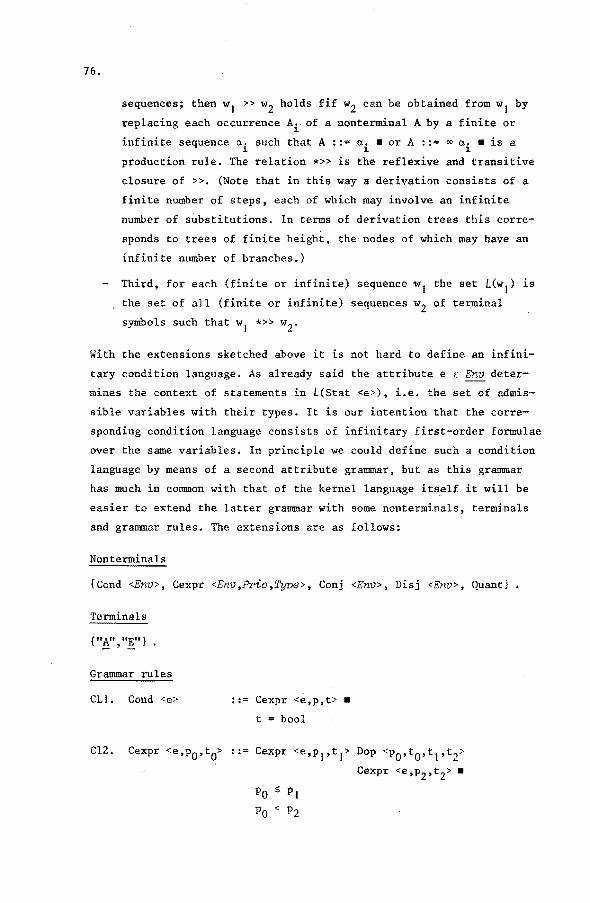
76.
sequences; then w1 >> w2 holds fif w2 can be obtained from w1 by
replacing each occurrence Ai of a nonterminal A by a finite or
infinite sequence ai such that A::= ai • or A::= oo ai • is a
production rule. The relation *>> is the reflexive and transitive
closure of >>, (Note that in this way a derivation consists of a
finite number of steps, each of which may involve an infinite
number of substitut~ons. In terms of derivation trees this corre
sponds to trees of finite height, the nodes of which may have an
infinite number of branches.)
Third, for each (finite or infinite) sequence w1 the set L(w1} is
the set of all (finite or infinite) sequences w2 of terminal
symbols such that w1 *>> w2.
With the extensions sketched above it is not hard to define an infini
tary condition language. As already said the attribute e E Env deter
mines the context of statements in L(Stat <e>), i.e. thesetof admis
sible variables with their types. It is our intention that the eerre
sponding condition language consists of infinitary first-order formulae
over the same variables. In principle we could define such a condition
language by means of a second attribute grammar, but as this grammar
has much in camman with that of the kernel language it~elf it will be
easier to extend the latter grammar with some nonterminals, terminals
and grammar rules. The extensions are as follows:
Nonterminals
{Cond <Env>, Cexpr <Env,Prio,Type>, Conj <Env>, Disj <Env>, Quant} •
Terminals
Grammar rules
CLI. Cond <e> ::= Cexpr <e,p,t> •
t = bool
Cl2. Cexpr <e,p0 ,t0> ::= Cexpr <e,p 1,t 1> Dop <p0,t0,t
1,t2>
Cexpr <e,p2,t2> •

CL3. Cexpr <e,p0 ,t0> ::=Mop <t0,t 1> Cexpr <e,p 1,t 1> •
Po 7 PI = 7
CL4. Cexpr <e,p0
,t> ::= (Cexpr <e,p 1,t>) •
Po = 1
CL5. Cexpr <e0
,p0
,t> ::= (Quant Decs <d> I Cexpr <e1,p
1,t>
I Cexpr <e 1,p2 ,t> •
CL6. Cexpr <e,p,t>
CL7. Cexpr <e,p,t>
CL8. Cexpr <e,p,t>
CL9. Cexpr <e,p,t>
t = bool
(! n: Name I #D (n,d) $ I)
::=Var <e,n,t> •
p = 7
::=Con <t> •
p = 7
: := Disj <e> •
p = 2
t bool
: := Conj <e> •
p 3
t = bool
CLIO. Let a be such that dom(a) = IN and for all i: 0 $ i:
a2i = Cexpr <e,p,t>, a2i+l = v
Disj <e> ::==-co (l. p > 2
t bool
CLII. Let a be such that dom(a) =IN and for all i: 0 $i:
a 2i = Cexpr <e,p,t>, a 2i+l = A •
Conj <e> ::=co a• p > 3
t bool
77.

n.
CLI2. Quant : := A o
CLI3. Quant : := E o
The condition language that may be used with L(Stat <e>) is now simply
defined as L(Cond <e>)." By induction it is nothard to prove that for
all e E Env, p E Prio:
L(Expr <e,p,bool>) ~ L(Cond <e>) •
Example
Let d E Deas, e = Ext(Empty,d) be such that
Prog
I[ var Decs <d> I Stat <e> ] I
I[ var x,y: int,b: bool I Stat <e> ]I
The set L(Stat <e>) contains elements like
skip
b := x > 3
x,y := 0,0; do x~ 10 +x:= x+ I; y := y +x* x od
but not
c := 3
b := x + l
x + skip fi •
The set L(Cond <e>) contains elements like
true
b V X > y
<~ z: int I z < x I z < y)
but not

x
b > 3
(~ a: bool I true I a > 3) •
0
No te
In the sequel we will usually abbreviate conditions of the form
(~ x: t true I q) or (!:_ x: t I true I q) to (A x: t 11 q) and
(~x: t
0
No te
q), respectively.
79.
We will often have to reason about conditions that are conjunctions or
disjunctionsof the elementsof a countable set Q ~ L(Cond <e>). We
will denote such conditions by /\Q and VQ respectively.
In case Q is a finite set such as {qi E l(Cond <e>) ~ i ~ n} we
will also write [(\i I I ~ i "; n I q.) and [V i I I s i ~ n I q.] l. l.
respectively.
In case Q is an infinite set such as {qi E L(Cond <e>) I I s i} we
will also write [/\i I I si I q.] and [Vi I I si I q.], respectively. l. l.
It should be borne in mind that these notations are just abbreviations
and do not themselves belong to the condition language!
0
3.2.2. The logic D
Calculations with conditions will be based upon a logic called D. The
logic D differs from ordinary first-order predicate logic in two
respects. First, like L it allows for infinitary formulae and proof WJW
rules to handle these. Second, it reflects that conditions are only
meaningful relative to a certain context. The formulae of D are of the
form cjp, where c is a sequence of declaration parts corresponding to
an attribute e E Env and p is an element of L(Cond <e>). More precisely,
the set of formulae is the set L(Form <Env>) defined by the extensions
below to the attribute grammar for the condition language. As prepara-'
tion for manipulations with contexts in theorem 3.54 and in chapter 4
these extensions also contain two operations, new and rep, on environ
ments. new(x,e) indicates that a name x does not occur in an environ-

80.
ment e. rep(e,e',x,x') indicates that e' differs from e only in that
each occurrence of x is replaced by x'. It will only be used with x'
such that new(x',e) holds. The extensions follow.
Operations on Env
new(•,•) Name * Env + Boot
rep(·,·,•,•): Env * Env *Name* Name+ Boot
new(x,e) ï (~ t: Type (x,t) e)
rep(e,e',x,x') = (~ y: Name,t: Type
y f x A y f x'
A (~ t: Tyve I (x,t)
Nonterminals
{Form <Env>, Cont <Env>}
Terminals
{"t>"}
Grammar rules
Form <e> ::= Cont <e> I Cond <e> •
Cont <e> : := •
e = Empty
(y,t) i~·e • (y,t) ~ e')
e • (x',t) inE e') •
Cont <e0> ::= Cont <e 1> > Decs <d> •
e0 = Ext(e 1 ,d)
Examples
1> x,y: int 1> b: bool I b ~x > y
1> x,y: int (~ b : boo 1 11 b ~ x > y)
(~ x,y: int 11 (~ b: bool 11 b,. x > y))
1> x,y: int I x > y
D
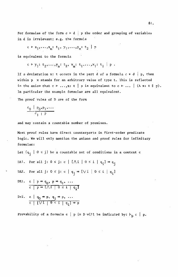
81.
For formulae of the form c ~ d I p the order and grouping of variables
in d is irrelevant; e.g. the formula
is equivalent to the formula
p •
If a deelaratien x: t occurs in the part d of a formula c ~ d I p, then
within p x stands for an arbitrary value of type t. This is reflected
in the axiom that c 1> ••• ,x: t I p is equivalent to c ~ • • • I (A x: t 11 p).
In particular the example formulae are all equivalent.
The proef rules of D are of the form
cO Po•PJ>'''
cl I P
and may contain a countable number of premises.
Most proof rules have direct counterparts in first-order predicate
logic. We will only mention the axioms and proef rules for infinitary
formulae:
Let {q. I 0 5 j} be a countable set of conditions in a context c J
DAl. For all j: 0 5 j: c [/\i I os i I q.J .. q. ~ J
,, DA2. Forallj: Osj: c I q.•(Vi I Os i I q.] J ~
DRI. c 1 P .. q0 , p .. q1,
c 1 p .. rA i 1 o s i 1 qi 1
Dr2. c I q0 =~> p, q1 • p, •••
c I [V~ I 0 s l I qi] =I> p
Provability of a formula c I p in D will be indicated by: ~D c I p.
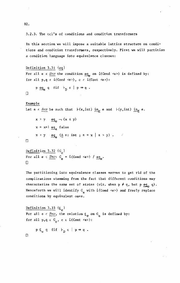
82.
3.2.3. The ccl's of conditions and condition transfarmers
In this section we will impose a suitable lattice structure on condi
tions and condition transformers, respectively. First we will partition
a condition language into equivalence classes:
Definition 3.31 {eq}
For all e E Env the condition =se on L(Cond <e>) is defined by:
for all p,q E L(Cond <e>), c E L(Cont <e>):
p q fif ~D c I p ~ q •
0
Example
Let e E be such that ~(x,int) ~ e and ~(y,int) ~ e.
x > y =se --, (x s y)
x x+l =se false
x > y (A z: int I z x 1 z > y) •
0
Definition 3.32 {Ce}
For all e E Env: C e L(Cond <e>) I =se· 0
The partitioning into equivalence classes serves to get rid of the
complications stemming from the fact that different conditions may
characterize the sameset of states (viz. when p ~ q, but p =se q).
Henceforth we will identify with L(Cond <e>) and freely replace
conditions by equivalent ones.
Definition 3.33 {c } -e For all e E Env, the relation ~e on
for all p,q € Ce' c E L(Cont <e>):
p ~e q fif ~D c I p ~ q •
0
is defined by:

Example
Let e be as in the previous example.
x > y c: x > y-l -e
x> y c: (! z: int I y > z I x > z) -e
false c: x > y -e D
It can easily be verified that ~e is a partial order on Ce. In fact:
Theorem 3.34
For all e E Env: (Ce,Ee) is a cel.
D
Proof
Let Q be a countable subset of Ce.
u Q \IQ, on account of definition 3.33, axiom DA2 and rule DR2.
n Q AQ, on account of definition 3.33, axiom DAl and rule DRI.
D
Note that, in particular:
J.c = u 0 false e
TC = n 0 true. e
Next we will impose a lattice structure on condition transformers.
Definition 3,35 {T } e
For all e E Env:
T C -+ C e e e
D
Theorem 3.36
Let e E Env. Let ~T be the standard order on Te. e
(Te'~T ) is a cel. D e
Proof
Immediately by theorem 3.10.2. D
83.

84.
3.2.4. Definitions and some properties of wp and wlp
The fact that for any e E Env both Ce and Te are ccl's enables us to
discuss the condition transformers wp and wlp in a lattice-theoretical
framework. We begin with presenting our versions of the definitions of
wp and wlp.
Definition 3.37 {wp}
Por all e E Env the function wpe E L(Stat <e>) +Te is defined by:
I. wpe (abort)
3. wpe(v := E) = (v + E) {see first note below}
5. 'lvp (if BI +SJ D ... 0 B _,. s fi) e- n n-
(Xq E: C I [Vi I lds:n IB.] A [;\i I l~is:n IB. •wp (S,)(q)]) e 1 1 e 1
A [;\i I ls:i~n I B. • wp (S.)(f(q))])) • l e l
Definition 3.38 {wlp}
Por all e E Env the function wlpe E L(Stat <e>) + Te is defined by:
3. wlpe(v := E) = (v + E) {see first note below}
(Xq E Ce I [;\i I IS:i~n I B . .,. wlp (S.}(q))) 1 e 1

85.
6. wlp (do B1 + s1 0 ... 0 B + S od) = vG, e- n n-
A [/\i I J:<:;i::;n I B • .,. wlp (S.) (f(q)) ])) l. e l.
0
No te
The operator {v + E) occurring in definitions 3.37.3 and 3.38.3 is an
instanee of the substitution operator for conditions, that we assume to
have been defined in the customary way with precautions to avoid name
clashes. See e.g. [Curry, de Bakker].
0
No te
In the sequel we will aften omit the brackets around the condition
argument of functions like wp and wlp, writing e.g. wpe(S 1)wpe(S2)q
insteadof wpe(s 1)(wpe(S2)(q)).
0
In definition 3.37.6 wp B1 + s1 U ... U B + S od) is weli-e n n-
defined only if the least fixed point ~f of F iudeed exists. According
to theerem 3.28.1 existence of uF is guaranteed if Fis upward continu
ous, which in its turn depends on upward continuity (and well-defined
ness:) of wpe(Si) for i: I ::; i s n. A similar remark applies to downward
continuity of G in definition 3.38.6.
Theerem 3.39 simultaneously states the continuity of wpe(S) and F {and
also that of wlpe(S) and G), thereby justifying the definitions above.
This theerem is the first of a number of theorems that express some
important properties of wp and wlp. Same of these are reformulations of
properties mentioned in [Dijkstra 2]. Most of the proofs make use of
both structural induction on the composition of statements and fixed
point induction. Induction hypotheses are indicated by the letter H and
an index.

86.
Theorem 3.39
For all e E
1 • wpe (S) E C
S E L(Stat <e>):
+ c e uc e
If S is of the form do Bl .,. SI
definition 3.37.6, then F E (C e
2. wlpe(S) E ... c . de e
If S is of the form do B1
+ s1
definition 3.38.6, then G E (C e 0
0 ... 0 B + S od, and F is n n-... c ) ... (C + Ce). uc e uc e ue
0 ... 0 B + S od, and G is n n-+de Ce) ...
de (Ce +de Ce) .
We only prove I. The proof of 2 is similar when dual versionsof
theorems 3.24 and 3.26 are used.
The proof is by induction on the composition of S.
I . I . S : : abort
Immediately by theorem 3.24.1.
1.2. S :: skip
Immediately by theorem 3.24.2.
I. 3. S :: v :s E
Let <q.>~ 0 be an ascending chain in Ce. ~ ~=
wpe(v := E)[Vi I 0 s; i I qi]
{definition 3.37.3}
(v + E)[Vi I 0 si I q.] ~
[Vi I 0 Si I (v+E)q.] ~
{definition 3.37.3}
[Vi I is 0 I wp (v+E)q.] e ~
Hl. wp e (SI) E Ce + uc Ce •
H2. wpe(S2) E Ce +uc Ce.
Immediately by theorem 3.24.3.
as in
as in

D
87.
1.5. s :: if B +SJ D ... D B + s fi - n n-
wpe (S)
{definition 3.37.5}
(Àq € C I [\/i I J";i";n I B.] A [Ai I J,çi";n I B. "* wp (S.)q]) e 1 1 e 1
= {prop. log.}
(Àq € Ce I [\/i I J,.;i,.;n I Bi] A [/\i I J,çisn I <Bi v wpe (Si)q])
From H3 and repeated application of theorem 3.24 it follows that
wp (S) € C + C • e e uc e
From H4 and repeated application of theerem 3.26 it fellows that
FE (C + Ce)+ (C + C ). e uc uc e uc e
Hence ~F exists and is an element of C + Ce' so e uc
For alleE Env, S"' L(Stat <e>):
D
D
I. wpe (S) "' C + C • e m e
2. wlpe(S) € C + C • e m e
s € L(Stat
I. wpe(S) is .1-strict.
2. wlpe(S) is T-strict.
<e>):

88.
Proof
We only prove 1; the proof of 2 is similar. Th~ proof is by induction
on the composition of S.
I • I.
l. 2.
I. 3.
I , 4.
s .. abort
Immediately by theerem 3. 13. 1 •
s .. skip
Immediately by theerem 3.13.2.
s .. V :g E
wp(v := E) false
{definition 3.37.3} (v + E} false
false.
s .. SI ;S2
Hl. wpe(Sl) is 1-strict.
H2: wpe (S2) is 1-strict.
wp(S 1;s2} false
{definition 3.37.4} wp(S1}wp(S2) false
{H2} wp(S 1) false
{Hl} false.
l. 5. s :: if + SI D ••• D +S fi n-
H3. For all i: I s is n: wpe(Si) is L-strict.
wp B1 + s1 D ••• 0 B + S fi) false n n-
= {definition 3.37.5}
[Vi I lsisn IB.] A [/\i 1
{H3} [Vi I lsisn I B.] 11 1
{prop. log.} false.
I lsisn I B. • wp (S.) false] 1 e 1
[/\i I lsisn I B. ,. false] 1
1.6. S :: do B1 + s1 0 ••• D B + S od - n n-
H4. For all i: I s i s n: wpe(Si) is 1-strict.
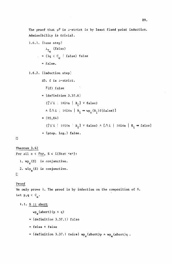
89.
The proof that ~F is ~-strict is by least fixed point induction.
Admissibility is trivial.
0
1.6.1. {base step}
~T (false) e
(Àq t C I false) false e
false.
1.6.2. {induction step}
HS. f is ~-strict.
f(f) false
{definition 3.37.6}
([Vi I J:s;i<;;n IB.] v false) l
A [;\i I J:s;i:s;n I B. => wp (S.)f(false)] 1 · e 1
m {HS,H4}
([Vi I ISiS:n I B.] v false) A [Ai I ]:s;i:s;n I B. => false] l l
{prop. log.} false.
Theorem 3.42
For alleE Env, St L(Stat <e>):
0
I. wp (S) is conjunctive. e
2. wlpe(S) is conjunctive.
Proof
We only prove I. The proof is by induction on the composition of S.
Let p,q t Ce.
l.I. S :: abort
wpe(abort)(p A q)
{definition 3.37.1} false
false A false
{definition 3.37.1 twice} wp (abort)p A wp (abort)q. e e

90.
1. 2. S : : skip
wp e (skip) (p A q)
{definition 3.37.2} p A q
= {definition 3.37.2 twice} wpe(skip)p A wpe(skip)q.
1.3.S::v:=E
wpe(v := E)(p A q)
{definition 3.37.3} (v + E)(p 1\ q)
(v + E)p A (v + E)q
{definition 3.37.3 twice} wpe(v := E)p A wpe(v := E)q.
Hl. wpe(S 1) is conjunctive.
H2. wpe(s2) is conjunctive.
wp(s1;s
2)(p 1\ q)
{definition 3.37.4} wpe(S 1)wpe(S2)(p A q)
{HZ} wpe(s 1)(wpe<s2)p A wpeCS2)q)
{Hl} wpe(Sl)wpe(S2)p A wpe(SI)wpe(Sz)q
= {definition 3.37.4 twice} wp(S1;s2)p A wp(s
1;s2)q
1.5. s :: ifB, .... SI D ....... B D s fi - n n-
H3. For all i: I s i s n: wpe(Si) is conjunctive.
wpe(S)(p A q)
{definition 3.37.5}
(V i I I:S:isn I B.] A [/\i I J:s:i:s:n I B. ""wp (S.)(p A q)] 1. 1. e 1.
{H3}
[Vi lsisn I Bi] A [/\i I IS:isn I Bi"" (wpe(Si)p A wpe(Si)q)]
{prop. log.}
[V i I Jsisn I B.] A [/\i I I:S:i:s:n I B. ""wp (S.)p] 1. 1. e 1.

0
91.
A [V i I l~hn I B.] A [/\i I lSiS1 I B. • wp (S.)q] l. l. e l.
{definition 3.37.5 twice} wpe(S)p A wpe(S)q •
1,6~ S ::do B1
+ s1 0 ••• DB + S od , - n n-
H4. For all i: l ~i ~ n: wpe(Si) is conjunctive.
The proof that ~F is conjunctive is by least fixed point induc
tion. Admissibility fellows from lemma 3.21.
1.6.1. {base step}
See 1. 1.
1.6.2. {induction step}
HS. f is conjunctive.
F(f) (p A q)
{definition 3.37.6}
([Vi I lsisn I B.] v (pA q)) ].
A [/\i I 1sisn I B. • wp (S.)f(p A q)] l. e l.
{H5,H4}
([Vi I Jsisn I B.] v (pA q)) ].
A [ 1\ i I 1 sisn B. • (wp (S.)fp A wp (S.)fq)] 1 e l. e 1
{prop. log.}
([Vi
A ([Vi
Jsisn Bi] v p) A [/\i
I sisn B,] V q) A [ 1\ i ].
l~isn B. • wp (S.)fp] l. e l.
lsisn B. • wp (S.)fq] l. e J.
= {definition 3.37.6 twice} F(f)p A F(f)q
Theorem 3.43
For alleE Env, SE L(Stat <e>), q E Ce:
0
Proof
The proof is by induction on the composition of S. Let q E Ce.

wpe(abort)q
{definition 3.37.1} false
{prop. log.} false À true
{definitions 3.37.1, 3.38.1} wp (abort)true À wlp (abort)q. e e
2. s ..
wp (skip)q e
{definition 3.37.2} q
{prop. log.} true À q
{definitions 3.37.2, 3.38.2} wpe(skip)true À wlpe(skip)q.
3. S :: V := E
wpe(v := E)q
= {definition 3.37. 3} (v + E)q
• {subst. prop. log.} (v + E)true À (v + E)q
= {definitions 3.37.3, 3.38.4} wpe(v := E)true À wlpe(v := E}q •
Hl. wpe(S 1)q = wpe(S 1)true A wlpe(S 1)q.
HZ. wpe(s2)q = wpe(s 2}true A wlpe(s2)q.
wpe(SI;Sz)q
{definition 3.37.4} wpe(S 1}wpe(S2)q
{Hl} wpe(S 1)true A wlpe(s 1)wpe(s2)q
{HZ} wpe(S 1)true À wlpe(S 1)(wpe(s2)true À wlpe(s2)q)
{theorem 3.42.2}
wpe(S 1)true À wlpe(S 1)wpe(s2)true A wlpe(S 1)wlpe(s2)
{Hl} wpe(s 1)wpe(s2)true À wlpe(s 1)wlpe(s2)q
{definitions 3.37.4, 3.38.4} wpe(s 1;s2)true A wlpe(s 1;s2)q.

5. S :: if B1 + s1 .0 ••• 0 B + S fi - n n-
H3. For all i: I ~ i ~ n: wp (S.)q = wp (S.)true A wlpe(S~)q. e ~ e ~ k
wpe(S)q
{definition 3.37.5}
[Vi J l~i~n I = {H3}
] A (/\i I l~i~n I B. ". wp (S.)q] 1 e ~
93.
[Vi l::;;i::;;n ] A [/\i I )::;;i::;;n I B. ". (wp (S.)true A wlp(S.)q)] ~ - e ~ ~ -
{prop. log.}
[Vi I
A [ 1\ i l~i::;;n B. ".wlp (S.)q] ~ e ~
{definitions 3.37.5, 3.38.5} wpe(S)true A wlp(S}q •
6. S :: do B1 + s1 0 ... 0 B + S od - n n-
H4. For all i: I ~ i ~ n: wpe(Si)q = wpe(Si)true A wlpe(Si)q.
The proof that (~F)(q) = (~F)(true) A (vG)(q) is by simultaneous
fixed point induction. Admissibility follows from lemma 3.44 below.
6.1. {base step}
.lT (q) e
(Àq E Ce I false)q
false
false A true
(Àq E Ce I false)true A (Àq E Ce I true)q
.lT (true) A (q) • e
6.2. finduetion step}
HS. f(q) = f(true) A g(q).
F(f) (g)
{definition 3.37.6}
([Vi I lsisn I B.] v q) A [/\i I lsisn I B. ". wp (S.)f(q)] ~ ~ e ~

94.
0
{H4,H5}
([Vi I tsisn I B.] v q) A [;\i I Isisn I B. • 1 1
(wpe(Si)true A wlpe(Si)(f(true) A g(q)))]
{theorem 3.42.2}
([Vi I tsisn I B.] v q) A [/\i I tsisn I B. • 1 1
(wpe(S1.)true A wlp (S.)(f(true)) A wlp (S.)(g(q)))] e 1 ·e 1
{H4}
([Vi I tsisn IB.] v q) A [;\i I lsisn IB. • 1 1
(wpe(Si)(f(true)) A wlpe(Si)(g(q)))]
{prop. log.}
([Vi I Jsisn I B.] v q) 1
A [;\i I Jsisn IB. •wp (S.)(f(true))] 1 e 1
A ([Vi I tsisn IB.] v q) 1
A [/\i I Jsisn IB. :o-wlpe(S.)(g(q))] 1 1
{definit.ions 3.37.6, 3.38.6} F(f)(true) A G(g)(q) •
The admissibility for simultaneous fixed point induction in proof 3.43.6
is an immediate consequence of the following lemma.
Lemma 3.44
Let (C,~) be a cel.
Let <fi>~=O and <hi>~=O be two ascending chains in (C,~). Let <gi>i=o be a deseending chain in (C,~).
If (A i I i~ 0 I f. = h~ n g.), then - 1 1 1
0

Pro of
f is ascending
<.! i I i :::: o I <.! j I j 2 i I j I j ;::: o I r. h. n g.)}
J J J
c f.)) - J
<.! i I i :::: o I <.! j I j :::: i I r i !;. h j n g j > >
{definition glb}
<.! i I i ;::: o I <.! j
~ {definition lub, glb}
j 2 i fl.. ~ hJ. A f. C g.)) l. - J
(_! i I i ;::: 0 I fi E j~i hj A fi ~ jgi gj)
~ {h ascending, g descending}
(_! i I i ;::: 0 I fi ~ j~O hj A fi t jQO gj)
~ {definition glb}
(_A i I i ;::: 0 I fl.. !: .uo h. n .no g.) J"' J J"' J
~ {definition lub}
i~O fi ~ j~O hj n jQO gj
{renaming}
i~O !:. i~O hi n iQO gi '
2. t:û
true
{definition glb}
<A i 1 i 2 o 1 g. ~ .n0 g.) - l. ·- J"' J
~ {definition glb}
(A i I i 2 0 I h. n g. ~ h. n .no g.) - 1 l. - 1 J"' J
{(A i I i;::: 0 I f. = h. n g.)} - l. 1 l.
(_! i I i 2 o I fi J hi n jQO gj)
95.
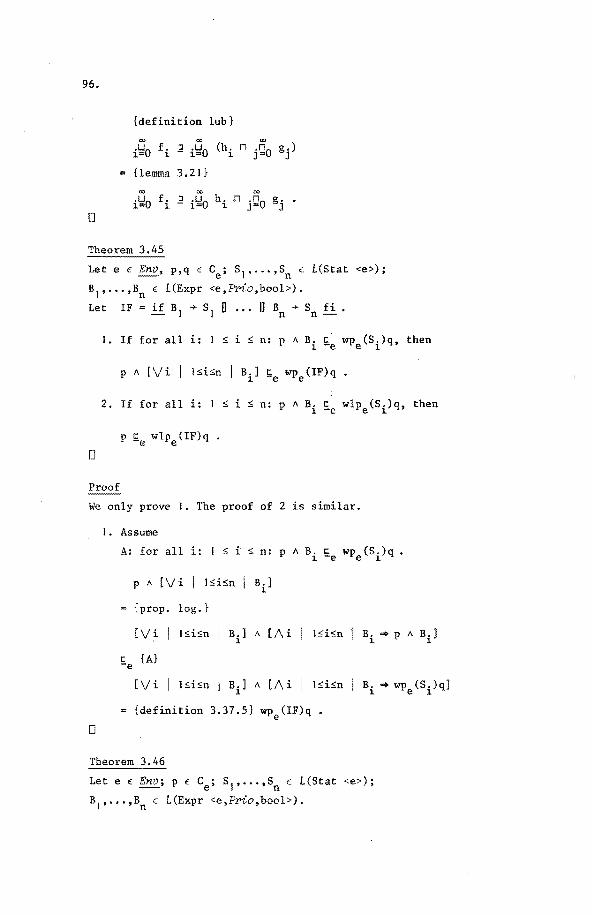
96.
0
{definition lub}
fi ~ i~O (hi n jQO gj)
{lemma 3.21}
Theorem 3.45
Let e E p,q E Ce; sl, ... ,sn L(Stat <e>);
B1
, ••• ,Bn E L(Expr <e,Prio,bool>).
Let IF = if B1
..,. s1
0 ••• I] B ..,. S fi . - n n
I. If for all i: I
D
s i s n: p A B. c wp (S.)q, then l. -e e J.
\ve only prove I. The proof of 2 is similar.
D
I, Assume
A: for all i: I <:; i $ n: p A Bi Se wpe(Si)q •
pA [Vi I lsisn I B.] ].
{prop. log.}
[V i
{A}
J<:;i<:;n I B.] A [/\i I J<:;i<:;n I B.-. pA B.] l l ].
[V i I J<:;isn I B.] A [/\i I t::;;isn I B. -. wp (S. )q] 1 1 e 1
{definition 3.37.5} wp (IF)q • e
Theorem 3.46
Let e E Env; p E Ce; s 1, ••• ,sn E L(Stat <e>);
B1, ••• ,Bn E l(Expr <e,Prio,bool>),

Let BB "" [V i I I ::;i Sn. B. ] • ~
I. If for all i: I::; i::; n: pA Bi
p wlpe(DO)(p A • BB) •
0
Proof
We first prove 2, and subsequently I.
2. Assume
The proof that p (vG)(p A • BB) is by greatest fixed point
induction. Admissibility follows from definition 3.2.1.
2.1. {base step}
p
c: true -e
(;\,q E C I true) (p A -, BB) e
TT (p A -. BB) e
2.2. {induction step}
H: p Se g(p A -,BB)
G(g)(p A-, BB)
{definition 3.38.6}
(BB v (pA ï BB)) A [Ai I Js:i::;n I B.,. ~
{prop. log.}
wlp (S.)(g(p A-, BB))] e ~
(BB v p) A [Ai I l::;i::;n I B.,. wlp (S.)(g(p A-, BB))] ~ e ~
97.

98.
D
~e {H, corollary 3.40.2}
(BB v p) " [Ai I 1 sisn
.:1 {A2} -e
B.<$ wlp (S. )p] l. e l.
(BB v p) " [Ai I Jsisn I Bi • p "Bi]
{prop. log.} p •
I. Assume
By Al and theorem 3.43: for all i: 1 s i s n:
p AB. c wp (S.)true A wlp (S.)p , 1 -e e 1. e 1.
hence:
p A wpe (DO)true
c {Al' ,A2} -e
wlpe(DO)(p A •BB) A wpe(DO)true
{theorem 3.43}
wp (DO)(p A •BB) e
Theorem 3.47
Let e E Env; q E Ce; {p~ I a~ 0} a countable subset of Ce; s 1, ••• ,sn•
B1, ••• ,Bn, IF, DO, BB as in theorems 3.45 and 3.46.
I. wpe(DO)q = (q A..., BB) V wpe(IF)wp(DO)q .
2. If for all a: a ~ 0:
a. for all i: :5 is n: P~ AB. 1: wp (S.)[Va' l Osa'<a I p ,J ~ 1. -e e 1. a
b. Pa A ..., BB ~ q
then [Va. I a:?: 0 I pa] ~e wpe(DO)q.
D

Proof
D
I. wpe (DO)q
{definition 3.37.6, fixed point property}
(q v BB) A [/\i I J";isn I B. ,. wp (S.)wp (DO)q] l e l e
{definition BB, prop. log.}
(q 11-,BB) v (BB 11 [/\i lisün IB. ,.wp (S.)wp (DO)q )) 1 e 1 e
{definition 3.37.5}
(q 11 -, BB) V wp (IF)wp (DO)q e e
2. Let ~: ~ ~ 0. Consider
[\/~' I o~~· <~ I P~·] !;.e wpe (DO)q
,. {corollary 3.40.1}
wp (IF) [\/a' I Q";~• <~ I p , ] t: wp (IF)wp (DO)q e ~ -e e e
• {a, theorem 3.45}
p~ 11 BB Ëe wpe(IF)wpe(DO)q
- {b}
(p~ 11-, BB) v (p~ 11 BB) ~e (q 11-, BB) v wpe(IF)wpe(DO)q
{prop. log., I}
wp (DO)q • e
We have shown that for all a: ~ ~ 0:
hence by lemma 3.29:
99.

100.
3.3. Logies for partial and total correctness
In this section we will extend the logic D with additional formulae and
proof rules .that enable us to prove partial and total correctness
properties in the style of Hoare [Hoare I, Hoare 2]. We will also prove
consistency of these logies with respect to D. To this end we introduce
notions of validity and soundness. It should be noted that our use of
these terms differs from that in program correctness theory
[de Bakker, Cook 2] or formal logic. In the latter fields these notions
pertain to the relations with a model; in our case they pertain to
relations with the logic D.
Partial and total correctness formulae are introduced by the following
extensions to the attribute grammar for D-formulae.
Nonterminals
{Pform <Env>, Tform <Env>}.
Terminals
{ "{","}","[","]" }.
Grammar rules
Pform <e> ::= Form <e> •
Pform <e> ::= Cont <e> {Cond <e>} Stat <e> {Cond <e>} •
Tform <e> ::= Form <e> •
Tform <e> ::= Cont <e> [Cond <e>] Stat <e> [Cond <e>] •
Definition 3.48 {PvalidO, TvalidO}
On L(Pform <Env>) and L(Tform <EnV>), respectively, the predicates
PvalidO and TvalidO are defined as follows:
For all e E Env, c E L(Cont <e>), p,q E L(Cond <e>), S E S(Stat <e>):
l.I. PvalidO(c I p) = ~D c I p
1.2. PvalidO(c I {p}S{q}) = ~D c I p ~ wlpe(S)q.

2. 1. TvalidO(c I p) = ~D c I P •
2.2. TvalidO(c I [p]S[q]) =~De I p~wpe(S)q. 0
Definition 3.49 {proof rule}
D
I. A partial correctness proof rule is a construct of the form
f n
where n ?: I, and c0 I f 0 , ••• ,c0 I fn-l, c 1 I f E L(Pform <Env>).
2. A total correctness proof rule is a construct of the form
f n
wh!'!re n::: I, and c0 I f 0 , ••• ,c0 I fn-l' c 1 I f E L(Tform <Env>).
Definition 3.50 {PsoundO, TsoundO}
D
I. On partial correctness proof rules the predicate PsoundO is
defined by:
2. On total correctness proof rules the predicate TsoundO is defined
by:

102.
Definition 3.51 {PC0, PAI' .•• ,PA3, P~ 1 , ••• ,PR4 }
The partial correctness logic PC0 is defined by
- AxPCO = ~ u {PA1 ,PA2 ,PA3 }
- PrPC = PrD u {PR1,PR2 ,PR3 ,PR4 } 0
For all e E Env ,
c E L(Cont <e>) ,
p,q,q 1 ,q2,q
3,q
4 E L(Cond <e>) ,
B1, ••• ,Bn E L(Expr <e,Prio,bool>) ,
s,sl, ••• ,sn E L(Stat <e>) '
v, E such that v := E E L(Stat <e>)
PA1• c {true} abort {q}
PA2 • c {q} skip {q}
PA3. c {(v + E)q} v := E {q}
c I ql ~ q2• fqzl s {q3}, q3 • q4 PR 1• ----~--~--~----~--~----~
c I { q I } s { q4 }
c I {pA B1
} s1 {p} , ... , {pA Bn} Sn {p}
PR4• -------------------------------------------------------c I {p} do B1 + s1 0 ••• 0 Bn +Sn od {p A'-~[Vi I l~i~n I Bi]}
0
Theorem 3.52
I . For all ax E ~c : PvalidO(ax) . 0
2. For all pr E PrPC : 0
PsoundO(pr)
0

Proof
We only have to consider PA1, ... ,PA3, PR1, ••• ,PR4•
I. PvalidO(PA1), Pvalid0(PA2 ) and PvalidO(PA3) follow immediately
from definition 3.48.1.2 and definitions 3.38.1, 3.38.2 and
3.38.3, respectively.
2. I. case PR1
Assume Al. PvalidO(c ql =I> q2) •
A2. PvalidO(c {q2} s {q3})
A3. PvalidO(c q3•q4).
wlpe(S)q4
~e {A3, corollary 3.40.2} wlpe(S)q3
~e {A2} q2
{Al} q1
hence PvalidO(c I {q1
} S {q4}) •
2.2. case PR2
Assume Al. PvalidO(c {q1
} S1
{q2})
A2. PvalidO(c {q2} s2
{q3})
wlpe(SI;S2)q3
= {definition 3.39.4} wlpe(S1)wlp(S2)q3
{A2, corollary 3.40.2} wlpe(S1)q2
.:!e {Al} ql
hence PvalidO(c I {q 1} S1 ;s2 {q3}) •
2.3. case PR3
Assume for all i: Is is n: PvalidO(c I {pA B.} S. {q}), ~ ~
By thèorem 3.45.2:
PvalidO(c I {p} if B1 + s1 ll ••• D Bn + Sn fi {q}) .
103.

104.
2.4. case PR4
Assume for all i: 1 s i s n: PvalidO(c I {p A B.} S. {p}). l. l.
By theorem 3.46.2:
PvalidO(c I {p} do B1
+S1
0 ... 0 Bn+Sn od {pA ï[Vi 1 sisn I B.]} l.
0
Definition 3.53 {TC0 , TA 1, ••• ,TA3, TR1, ••• ,TR4 }
The total correctness logic TC0 is defined by
- AxTC = AxD u {TA1,TA2 ,TA3 } 0
- PrTCO = PrD u {TR1,TR2 ,TR3 ,TR4 }
where TA1
, ••• ,TA3
, TR 1, ••• ,TR4
are given below.
For all e E Env ,
c E L(Cont <e>) ,
p,q,q 1,q2,q3.q4 E L(Cond <e>) ,
B1
, ••• ,Bn E L{Expr <e,Frio,bool>) ,
S,S1
, ••• ,sn E L(Stat <e>) ,
v, E such that v := E E L(Stat <e>) ,
a E L(Expr <e,Frio,int>), A,E Name such that ~ new(A,e)
TA1
• c [false] abort [q]
TA2. c [q] skip [q]
TA3
• c [(v + E)q] v := E [q]
c I ql ~ q2' [q2] s [q3], TR1•
c I [ q I] s [q4]
c I [ql] SI [q2]' [q2] 5z TR2•
c I [ql] SI; [q3]
q3 ~ q4
[q3]
c I (p A BI] SI [q] , ... ,[pAB] n TR3• c I (p A lVi I lsisn I B.]] if B1 l. -
s [q] n
+ SI D ... D B + S fi [q] n n-

TR4• c ~A: int [p A B1 A O::;a A a=A) s1 [p A Osa A a<AJ
[p " " osa " a=A] [p " Osa " a<A]
0
Theerem 3.54
I • For all ax E AxTC : TvalidO(ax) 0
2. For all pr E PrTC : TsoundO(pr)
0 0
Proef
We only prove seundness of TR4; the other proofs are very similar to
those of theerem 3.52.
Let e' = Ext(e,[A,int]D).
for all i: I s i s n:
TvalidO(c ~ A: int I [p A B. A Osa A a=A] S. [p A Osa A a<A]) l. l.
{definition 3.48.2}
for all i: I s i s n:
~D c ~A: int I (p "Bi" Osa" a=A) • wpe,(Si)(p" Osa A a<A)
{axiom of D}
105.
~D c I (!:_A: int 11 (p " Bi A Osa " a=A) • wpe' (Si) (p " Osa " a<A))
0
• {*see note below}
for all i: I s i s n:
for all a: 0 s a:
~D c I (p" Bi " a=a) • wpe(Si)(p A Osa A a<ä)
• {definition 3.33, theorem 3.47}
[Vet I Osa I p" B. A a=~] c wp (DO)(p A rBB) . 1. -e e
pA Osa ~e wpe(DO)(p A, BB)
{definition 3.48.2}
TvalidO(c J [p A Osa] DO [p A, BB]) •

106.
In the step marked with a * we have applied the rule for A-elimination.
The notation a stands for an element of L(Con <int>) repreaenting the
value a. As in the resulting conditions·the variabie A no longer occurs,
wpe' may be replaced by wpe. Replacements of the latter kind will be
discussed more extensively ·in chapter 4.
0

CHAPTER I!
BLOCKS AND PROCEDURES
4.0. Introduetion
In this chapter we consider the design and formal definition of some
essential components of the souree language, viz. blocks and
procedures. We do so for various reasons:
107.
Blocks and procedures are nontrivial extensions to the kernel
language of chapter 3. They pose many interesting problems with
regard to the construction of correct compilers, which is the
ultimate goal of our studies.
In the literature on formal definitions in many cases the treat
ment of blocks and procedures is either incomplete or very
complex. The incompleteness usually results from consiclering
either the syntactic or the semantic aspects of the constructs,
whereas their interaction is often essential (e.g. in proof rules
for blocks, which critically depend on the scopes of variables).
The complexity usually results from consiclering an existing
procedure concept as it occurs in, say, ALGOL 60 or Pascal, as
holy, and trying to formalize all its aspects as faithfully as
possible, without questioning the quality of that concept. In
contrast, we want to define completely both syntax and semantics,
but we will try to design language constructs in such a way that
their definition is relatively simple.
It is interesting to investigate to what extent the condition
transfarmer method, which was designed for statements, can be
applied to more complex language constructs like recursive
procedures.
We will try to separate the various aspects as much as possible, and
to study their effect on syntax, semantics and proof rules. This
separation is reflected in the structure of the chapter. In sectien
4.1 we will discuss blocks, mainly to investigate the effects of the

!08.
introtluttion of local names. Section 4.2 deals wit.h parameter
mechanisms. The discussion is oase(! on a J.«ne•.t«g" construct cal led
ab~tnl'.'t.ion, which resembles the ALGOL 68 routinetext, and whic.h c.an
b" u~erl to stuóy the effects of paJ:ametrü<ttion, Se ct ion t,. 3 eon~f!n
tr~te~ nn reco~sion~ which c3n be handled rather e~sily by mean~ of
the L•ttic.~ theory of s~aion :1.1. Fin.•lly, in .•ec.tion 4.4 th" various
a..sreC'.ts ;1.re merged ~ re sult ing i.n a tr-er-~tment of parametrized recursivri!
proC'.edure.s. R;Jch sect:ton follows the S;JTfl.~ p:~.ttex-n of dis~u:!?.sing first
syntax~ then sem,qntic.c::~ and finally proof rules.

109.
4. I. lllocks
4. l.O. Intro<:luction
In sf!ction 4. I we <:liscuss the block, a constr\lct which provides the
rnf!ans for loeal extension of tho< f!rrvironment of statements. Although
the block is of some interest in its own right, our ~rime motivation
to discuss it is the desire to sepsrate th.o aspeet of the introduc.tion
of local nomenclature from other aspects of the proeedure concept.
From section 2. 3. 2 we reeall the [:p:amrnar rul<'> for bloc:ks:
2. Block <e0> r:= I[ var Does <d> I Stat <e 1> )I •
(!è_ n: Name I #D (n,d) ,; 1)
c 1 - Ext(~. 0 ,d)
Throughout section 4. I we shall restriet ourselves to blocks containin~
a sin~le variable doclaration, i.e. btocks of the forrn
I[ var x: t I S ] I. Generalization toother blocks is straightfo~ard.
In sectien 4. l.l we consider the case that re<:lecl.s>:ation is not allowed.
As a prepa>:ation for the treatm~nt of redeclaration in sectien 4.1.3
and for othe~ section~, seçtion 4. 1.2 is devoted to substitution in
progrsmrning language construct s. In sect ion 4. I. 4 proof ndes for
b1ncks are presented and their soundness is proven.
4. I, I, Blocks without >:edeclsration
In this section we stu<:ly the semantica of a block I[ var x: t I S] I
~ L(Block <e0
>) under the additional assumption that ~ new(x,e0 ), i.e.
that x has not been declarêd in surrounding block~. What we naed is a
definition of wpe (i[ var x! t I S ] I) in tcrms of ~De (S). Sincc it 0 - . l is our intf>ntion that I[ var x: t I S ll and S have thf> sameeffect as
far AS the variables of e0 are concerned, a definition of the following
forrn readity suggests itself:
wp (I[ var x: t eo
wp (S)q) el

110.
However, this definition is not always correct. Because e 1 is an
extension of e0 , Ceo is a proper subset of Cel' Therefore wpe 1(s) may
be applied to q, but the yield is not necessarily an element of Ceo•
since it might still contain x. A little reflection reveals that this
situation will only occur when x has not been initialized by S (where
for the moment we assume that we know what is meant by initialization).
There are at least two solutions to the problem:
I. Require that s es tablishes
of the initial value of x.
cation over x, as a result
element of Ceo:
wpe (I[ var x: tI S Jl) 0
the desired post-condition regardless
This boils down to universal quantifi-
of which the pre-condition becomes
(A x: t 11 wpe (S)q)) l
an
2. Impose the additional context condition that S initializes x.
Solution I does not fit well into the framework developed in chanter 3
because the resulting condition transfarmer is not upward continuous.
In the terminology of [Back l, Dijkstra 2] a block containing a
variabie of an unbounded type would be a construct of "unbounded non
determinacy"; e.g. the block I[~ y: nat I x:= y+l ]I would be an
implernentat:.ion of Dijkstra's "set x to any positive integer"
[Dijkstra 2]. Because of this complication we will notadopt salution I.
Salution 2 is in accordance with "disciplined" programming. Systematic
ally constructed programs will never contain uninitialized variables
and therefore we rnay as well exclude them syntactically. For the dura
tion of this chapter context conditions of this kind will be expressed
by means of some auxiliary functions defined below. Eventually they
will be incorporated into the attribute grammar for the souree language.
Definition 4. I {USE}
The function USE
L(Stat <Env>) u l(Expr <Env,PT'io,Tyve>) u l(Cond <Env>) + P(Name)
is defined recursively by
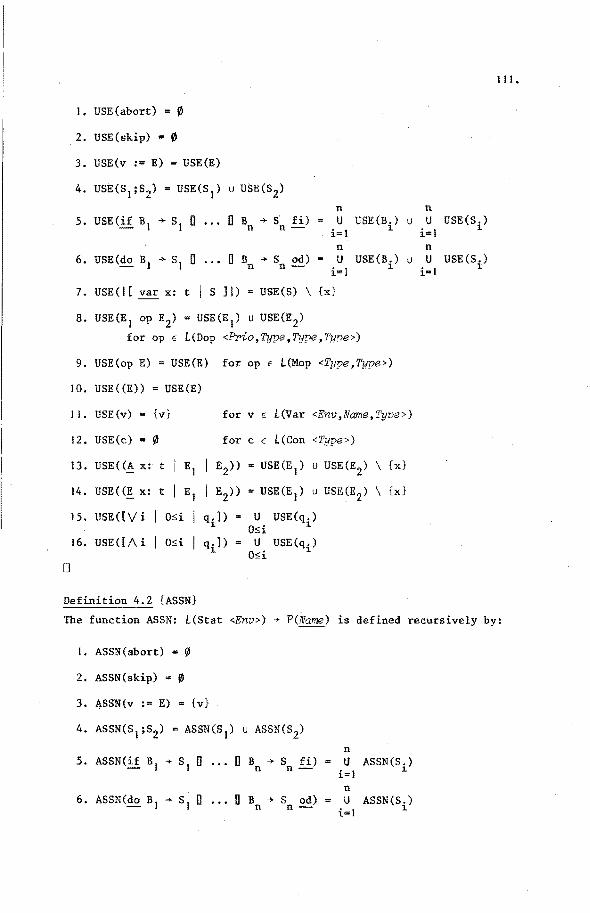
lil .
I • USE(abort) = 11)
2. USE(skip) = 0
3. USE(v := E) = USE(E)
4. USE(S 1;S2) = USE(S 1) u USE(S2)
n n 5. USE BI +SI 0 0 B + s fi) n n- u USE(Bi) u u USE(Si)
i=l i=l n n u USE(Bi) u u USE(Si)
i=! i=l
7. USE(I[ var x: t I S ]I)= USE(S) \{x}
8. USE(E 1 op E2) USE(E 1) u USE(E2)
for op € L(Dop <Prio,T.ype,Type,Tyrye>)
9. USE(op E) = USE(E) for op E L(Mop <Type,Type>)
10. USE((E)) = USE(E)
11. USE(v) = {v} for v E L(Var <Env,Name,Tyve>)
12. USE(c) = ~ for c E L(Con <Type>)
13. USE((A x: t E1
E2)) = USE(E
1) u USE(E
2) \ {x}
14. USE((! x: t E1
E2)) = USE(E
1) u USE(E
2) \ {x}
15. USE([V i q.]) l.
= U USE(q.) Od 1
16. USE([/\ i = U USE(q.) Osi 1
0
Definition 4.2 {ASSN}
The function ASSN: L(Stat <Env>) + P(Name) is defined recursively by:
I. ASSN(abort) = ~
2. ASSN(skip) = 0
3. ASSN(v := E) {v}
4. ASSN(S 1;s2) = ASSN(S 1) u ASSN(S2)
n 5. ASSN(if B1 +SI 0 0 B + S fi) u ASSN(S.) n n- i=l ].
n 6. ASSN(do B1 + s1 0 ... 0 B + S od) = u ASSN(Si) n n- i= I

112.
7. ASSN(I[varx: tI S ]I) =ASSN(S) \{x}
[]
Definition 4.3 {INIT}
The function INIT: L(Stat <Env>) 7 P(Name) is defined recursively by:
I. INIT(abort) = 0
2. INIT(skip) 0
3. INIT(v := E) {v} \ USE(E)
4. INIT(S 1;s2
) = INIT(S1) u (INIT(S
2) \ USE(S 1))
n n 5. INIT(if BI _.. SJ u u B ... s fi) n INIT(Si) \ u USE(Bi) n n- i= I i=l
6. INIT(do B1 -+ SI 0 0 B ... s 0 n n
7. INIT( I [ var x: t I S ] I) = INIT(S) \ {x}
0
Informally, for a construct c the set USE(c) may be interpreted as the
set of variables occurring in an expression in c, ASSN(c) as the set
of variables occurring in the left-hand side of an assignment in c,
and INIT(c) as the set of variables initialized by c, i.e. assigned to
by every possible execution of c and no~ used in any expression befare
they have been assigned to. The set USE(c) u ASSN(c) is the set of
"free" variables of c.
Example
Let S be the statement
D
x : 0; if x ~ y -+ y := 0; z := 0 0 true -+ w := w; z := x fi
USE(S)
ASSN(S)
INIT(S)
{x,y,w}
{x,y,z,w}
{x,z} •

Lemma 4.4
For alleE Env, SE L(Stat <e>):
I. INIT(S) ~ ASSN(S) •
2. ASSN(S) ~ {n E Name I (~ t e: ~·I ~ (n,t) inE e)} •
3. USE(S) s {n E Name (~tE I ~ (n,t) e)}.
0
Proof
By induction on the composition of statements. Details omitted.
0
Now consider again the proposed definitions
wp (I[ var x: t I S ]I); (Àq E Ce I wpe (S)q) eo - 0 I
wlpe (I[ var x: tI S ]I)= (Àq e: Ce I wlp (S)q) 0 - 0 el
113.
By induction on the composition of statements and the nesting depth of
blocks it can easily be seen that these definitions are well-formed
(i.e. wpe (S)q E C and wlpe1
(S)q E Ce0
> if we impose the additional I eo
context condition:
I x E INIT(S) V x t USE(S) I A similar condition is formulated in [de Bakker].
For future reference we collect some properties of USE, ASSN, and INIT
in the following lemma.
Lemma 4.5
For alleE Env, SE L(Stat <e>), p,q E L(Cond <e>):
I. USE(wpe(S)q) ~ USE(S) u USE(q) •
2. USE(wlpe(S)q) S USE(S) u USE(q)
3. USE(wpe(S)q) n INIT(S) = 0 .
4. USE(wlpe(S)q) n INIT(S) = 0 .
5. If ASSN(S) n USE(p) ; 0, then wp (S)(p A q) =pA wp (S)q. e e
6. If ASSN(S) n USE(p) = 0, then wlp (S) (p A q) = p A wlp (S)q. e e 0

114.
Pro of
By induction on the composition of statements. Details omitted.
[j
4.1.2. Substitution in statements
In the sequel we will sametimes define the meaning of a construct in
terros of the meaning:of a second construct derived from the first one
by a process invalving systematic replacements of variables. Such an
approach requires a precise definition of systematic replacement. Here
we present such a definition, much resembling those in [Curry, de
Bakker].
Definition 4.6 {(x+ y), substitution in statements}
For all x,y E L(Var <Env,Name,Type>) the substitution operator (x+ y)
on L(Stat <Env>) u L(expr <En1J,Prio,Type>) is defined recursively by:
I. (x+ y) abort = abort
2. (x + y) skip & skip
3. (x+ y)(v := E) = (x+ y)v := (x+ y)E
4. (x+ y)(S1;s
2) = (x+ y)S
1;(x + y)S
2
5. (x+ y) if B1
+ s1
D ••• 0 B + S fi = n n-
if (x+ y)B 1 +(x+ y)S 1 D ... D (x+ y)Bn +(x+ y)Sn fi
6. (x+ y) do B1 + s 1 D •.. DB + S od n n-
do (x-<- y)B 1 + (x-<- y)S 1 IJ ... D (x+ y)Bn + (x+ y)Sn od
7.
I. if x= w, then
(x + y) I [ var w: t I s 11 I [ var w: t I s ll
2. ifx 1' w and y 1' w, then
(x+ y) I [ var w: t I s ] I I [ var w: t I (x + y)S ] I
3. if x 1' w and y = w, then
(x +- y) I [ var w: t I s Jl I[ var z: t I (x+ y)(w + z)S ]I
where z is the first element (in some suitable ordering) of

L(Var <Env,Prio,Type>) such that
z i {x,y} u USE(S) u ASSN(S) •
8. (x+ y)(E1
op E2
) = (x+ y)E 1 op (x+ y)E2
9. {x<-y){opE) =op (x+y)E
10.
I. (x+y)z y
2, (x + y)z = z
IJ. (x+ y)z = z
0
if x = z } z E L(Var <Env,Prio,Type>)
if x "' z
z E L(Con <Type>)
115.
We reeall from section 3.2.4 that we assume that for conditions sub
stitution has been defined in the customary way. Without proof we state
the following obvious property.
Lemma 4. 7
For all x,y E L(Var <Env,Name,Tyve>), sE L(Stat <Env>),
c E L(Expr <Env,Prio,Type>) u L(Cond <Type>):
if x t/. USE(s) u ASSN(s), then (x+ y)s s •
if x i USE(c), then (x+ y)c = c.
0
The following lemma relates the condition transfermers of a statement
S and a statement S' obtained from S by systematic replacement of a
variable x by a variable x'.
Lemma 4.8
Let e E Env, S E L(Stat <e>),
Let x,x' E Name such that ~ -, new(x,e), ~ new(x' ,e).
Let 'e' E Env such that ~ rep(e,e' ,x,x').
Let S' = (x+ x')S.
0
I. wpe (S)
2. wlpe(S)
(x'+ x) o wp ,(S') o (x+ x') e
(x' +x) o wlpe 1 (S 1 ) o (x+ x')

116.
Proef
By induction on the composition of statements. Details omitted.
0
The following diagram may help in understanding lemma 4.8:
(x' + x)
1p E C e~----'---------'----------1 p ' E Ce ,
wp,(s) 1 wp,,(s')
q E C ef----(,...x_+_x':"'' ),....--_., ... q' E Ce'
Lemma 4.8 will now be used to prove the following lemma, which states
that' the local variable of a bleek may be replaced by a different
variable without affecting the meaning of the bleek, provided that the
replacement does not lead to violatien of the condition on redeclara
tion. This replacement is comparable to the a-conversion of lambda
calculus.
Lemma 4.9
Let e E Env, y E Name such that ~ new(y,e).
Let I[ var x: t I S ]I E L(Stat <e>).
0
I. wpe (I[ var x: t
2. wlpe(l[ var x: t
Pro of
We only prove I.
S ]I)= wpe (I[ var y: t
S ]I) = wlpe (I [ var y: t
(x + y) S ] I)
(x + y) S ]I)
Let e 1 = Ext(e,[x,t]D)' e2 = Ext(e,[y,t]D). Let q E Ce.
wp (I[ var x: t I S ]l)q e --
{proposed definition in sectien 4 .• I. I}
wpel (S)q
{lemma 4.8}
(y + x)wpe ((x+ y)S)(x + y)q 2

{x i USE (q), lemma 4. 7}
(y + x)wpe2
((x + y)S)q
117.
{y E INIT((x+y)S) v y i USE((x+y)S), y i USE(q), lemmas 4.5, 4,7}
wpez<<x + y)S)q
= {proposed definition in sectien 4.1.1}
wp (I[ var y: t I (x+ y)S ]l)q. e -D
4.1.3. Blocks with the possibility of redeclaration
Finally wedefine thesemantics of a block I[ var x: t IS ]I
E L(Block <e0>) without the restrietion ~ new(x,e0). In this case the
proposed definitions of sectien 4.1.1 are not directly applicable as
they could result in name clashes between the local x of a block and a
nonlocal x. Considering the purport of lemma 4.9, viz. that within
certain limits the meaning of a block is not affected by systematic
replacement of the local variable, we are led to the following solution:
Definition 4.10 {wp and wlp for blocks}
For all e0 E Env, I[ var x: t I S ]I E L(Block <e0>) such that
x E INIT(S) V x i USE(S):
I. wpe (I [ var x: t I S ] I) 0 -
2. wlpe0
(1[ var x: t I S ]I)
where, in both cases,
(Àq E CeO wpe1((x + y)S)q) 0
(Àq E CeQ wlpe1((x + y)S)q) ,
y E Name such that ~ new(y,e0)
e 1 = Ext(e0 ,[y,t]D) •
D
No te
It can easily be shown that the theorems of sections 3.2.4 and 3.3
also hold when the kernel language is extended with blocks as defined
in this section. We will not give these proofs, but we will freely use
the theorems where appropriate.
D
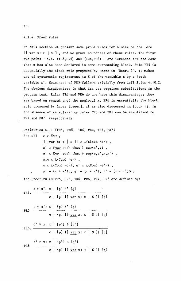
1!8.
4. 1.4. Proof rules
In this section we present some proof rules for blocks of the form
I[ var x: t I S ]1, and we prove soundnessof these rules. The first
two pairs - i.e. (TRS,PRS) and (TR6,PR6) - are intended for the case
that x has also been declared in some surrounding block. Rule PRS is
essentially the block rule proposed by· Hoare in [Hoare 2]. It makes
use of systematic replacement in S of the variabie x by a fresh
variabie x'. Soundnessof PRS follows trivially from definition 4. 10.2.
The obvious disadvantage is that its use requires substitutions in the
program text. Rules TR6 and PR6 do not have this disadvantage; they
are based on renaming of the nonlocal x. PR6 is essentially the block
rule proposed by Lauer [Lauer]; it is also discussed in [Cook 2]. In
the absence of redeclaration rules TRS and PRS can be simplified to
TR7 and PR7, respectively.
Definition 4.11 {TRS, PR5, TR6, PR6, TR7, PR7}
For all e E Env ,
I [ var x: t I s ]I E L(Block <e>) • x' E Name such that ~ new(x' ,e) • e' E Env such that ~ rep ( e, e' , x, x' )
' p,q E L(Cond <e>)
' c € L(Cont <e>), c' E L ( Cont <e' >) ,
p' = (x+ x')p, q' = (x+ x'), s• (x + x' )S ,
the proof rules TRS, PRS, TR6, PR6, TR7, PR7 are defined by:
c t> x': t [p] S' [q] TRS.
c I [p] I [ var x: t I s ]I [q]
c 1> x': t I {p} S' {q} PRS
c I { p} I [ var x: t I s ] I {q}
C I I> x: t [p'] s [q'] TR6.
c I [p] I [ var x: t I s ] I [q]
c' 1> x: t I {p'} s {q'} PR6
c I {p} I [ var x: t I s ]I {q}
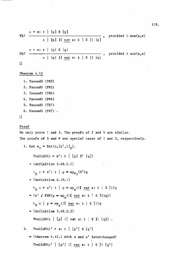
c l> x: t [p] s [q] TR7 provided ~ new(x,e)
c I [p] I [ var x: t I s ] I [q]
c l> x: t {p} s {q} PR7 provided ~ new(x,e)
c I {p} I [ var x: tiS]I{q}
0
Theerem 4.12
I. TsoundO (TR5)
2. PsoundO (PR5)
3. TsoundO (TR6)
4. PsoundO (PR6)
5. TsoundO (TR7)
6. PsoundO (PR7)
0
Proof
We only prove and 3. The proofs of 2 and 4 are similar.
The proofs of 5 and 6 are special cases of and 3, respectively.
I. Let e 1 = Ext(e,[x',t]D).
TvalidO(c 1> x': t I [p] S' [q])
{definition 3.48.2.2}
~D c 1> x': t I p ~ wpe1(S')q
{definition 4.10. I}
~D c 1> x': t I p ~ wpe(l[ var x: t I S ]l)q
{x' i USE(p ~ wp (I[ var x: t I S ]l)q)} e -
~D c I p~wpe(l[ var x: tI S ]l)q
{definition 3.48.2.2}
TvalidO(c I [p] I [ var x: t I S ] I [q]) .
3. TvalidO(c' 1> x: t I [p'] S [q']
~ {theorem 4.12.1 with x and x' interchanged}
TvalidO(c' I [p'] I[ var x: tI S ]I [q']
119.

120.
D
{definition 3.48.2.2}
~D c' I p' • wpe,(l[ ~x: t I S ]l)q'
{definition 4.6.7.1}
1-0 c' I p' • wpe·'((x +x') I[ var x: tI S ]l)q'
{~ new(x,e 1 )}
1-0 c I (x'+ x)p' • (x'+ x)wpe,((x +x') I[ var x: tI S ]l)q'
{definition p',q'; lemma 4.8.1}
~D c I p • wpe (I [ var x: t I S ] l)q
{definition 3.48.2.2}
TvalidO(c I [p] I [ var x: t I S ] I [q]) •
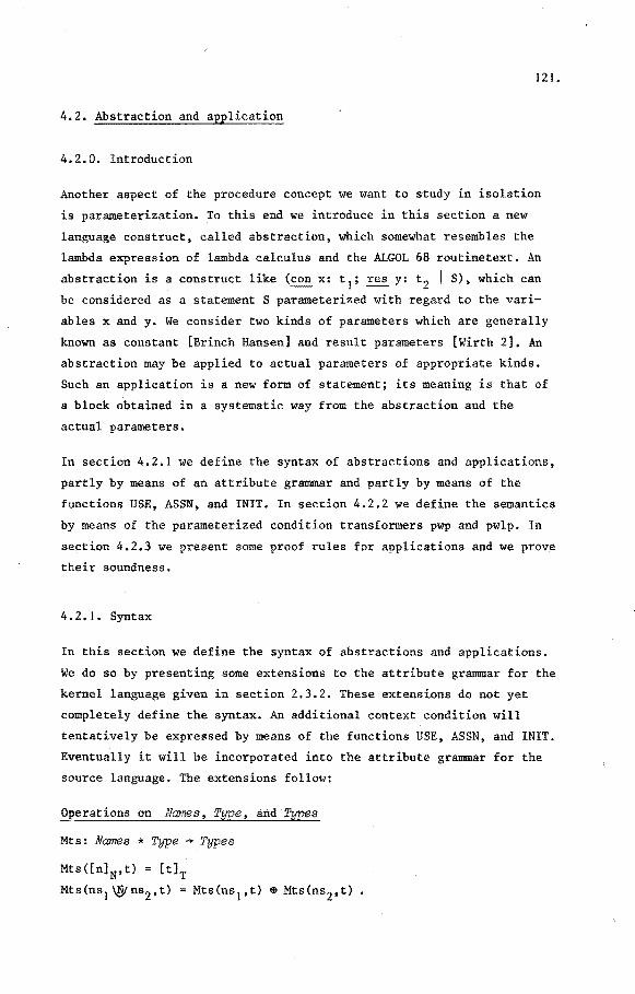
121.
4.2. Abstraction and application
4.2.0. Introduetion
Another aspect of the procedure concept we want to s·tudy in isolation
is parameterization. To this end we introduce in this section a new
language construct, called abstraction, which somewhat resembles the
lambda expression of lambda calculus and the ALGOL 68 routinetext. An
abstraction is a construct like (con x: t 1; res y: t 2 I S), which can
be considered as a statement S parameterized with regard to the vari
ables x and y. We consider two kinds of parameters which are generally
known as constant [Brinch Hansen] andresult parameters [Wirth 2]. An abstraction may be applied to actual parameters of appropriate kinds.
Such an application is a new form of statement; its meaning is that of
a block obtained in a systematic way from the abstraction and the
actual parameters.
Insection 4.2.1 wedefine the syntax of abstractions and applications,
partly by means of an attribute grammar and partly by means of the
functions USE, ASSN, and INIT. In section 4.2.2 we define the semantica
by means of the parameterized condition transfermers pwp and pwlp. In
section 4.2.3 we present some proof rules for applications and we prove
their soundness.
4.2.1. Syntax
In this section we define the syntax of abstractions and applications.
We do so by presenting some extensions to the attribute grammar for the
kemel language given in section 2.3.2. These extensions do not yet
completely define the syntax. An additional context condition will
tentatively be expressed by means of the functions USE, ASSN, and INIT.
Eventually it will be incorporated into the attribute grammar for the
souree language. The extensions follow:
Operations on Names • Type. artd Types
Mts: Narnes * Type -+ Types
Mts([n)N,t) = [t]T
Mts(ns 1 \!:Jins2,t) = Mts(ns 1,t) • Mts(ns2,t).

122.
{Infomally, Hts(ns,t) yields a sequence the elements of which all
equal tand the lengthof which equals the number of narnes in ns.}
Nonteminals
{Abstr <Types,Types>, Pdecs <Dees,Types>}
{"con","res"}
rul es
Al. Stat <e>
A2. Abstr <ts 1,ts2>
A3. Pdecs <d0,ts0>
A4. Pdecs <d,ts>
::= Abstr <ts 1,ts2> ( Exprs <e,ts 1>
Vars <e,ns,ts2> ) •
(~ n: Name I #N (n,ns) $ I)
: ;:::: con Pdecs <d 1,ts 1> res Pdecs <d2,ts2>
Stat <e 1> ) •
(~ n: Name I # (n,d 1 \J)/d2) :S I) D el = Ext(Empty,d 1 I.QJd2)
: := Pdecs <d 1,ts 1> '
Pdecs <d2,ts2> •
do = dl \Wdz
ts0 = ts 1 61T ts2
::= Ids <ns> : Type <t> •
d = [nd,t]D
ts = Mts(ns,t)
An abstraction - i.e. an element of L(Abstr <Types,Types>) - is a con
struct of the fom (con pd 1; res pd2 I S), where pd 1 and pd2 are
parameter declarations- i.e. elementsof L(Pdecs <Deas,Types>)- and S
is a statement. In the parameter declarations the formal parameters and
their types are listed. By means of the symbols "con" and "res" the
formal parameters are classified as constant and result parameters,
respectively. Their narnes must be mutually different. These narnes are
the only variable narnes that may occur in S. In other words, S has no

123.
access to nonlocal variables. Below we will formulate some additional
restrictions. An abstraction may be applied to actual parameters of
corresponding kind and type. An actual constant parameter is an expres
sion; an actual result parameter is a variable. Actual result parame
ters must be mutually different.
0
Example
The following is an element of L(Stat <Env>) as defined by the exten
sions above:
(con b: bool,x,y: int; res z: int 1· if b + z := x-y 0 ., b + z := y-x fi)
(true,3,a+4;c)
0
Abstractions have to satisfy some additional conditions, viz. that the
constituent statement does not assign to the constant parameters, and
that it initializes the result parameters. Like we did for blocks, we
will formulate these conditions in terms of the functions USE, ASSN,
and INIT. Before we do so we have to extend the definitions of these
functions to applications. As preparatien for section 4.2.2 we also
extend the definition of substitution.
Definition 4.13 {U~E,ASSN,INIT}
For all A(E 1, ... ,Em;v 1, ••. ,vn) E L(Stat <Env>):
m U USE(E.)
i=l ~
{vl' ... ,vn}
m {v1, ••• ,v} \ U USE(E.) •
n i=;1 l
0
Definition 4.14 {(x+ y), substitution}
For all x,y E L(Var <Env,Name,Type>),
A(E 1, ••• ,Em;v1, ••• ,vn) E L(Stat <Env>):
(x+ y)(A(E 1, ... ,Em;v 1, ... ,vn)) =
= A((x + y)E 1, ••. ,(x + y)Em;(x + y)v 1, ••• ,(x + y)vn)
0

124.
Note that no substitution inside the abstraction A is needed because
its statement does not access global variables.
The additional context condition for abstractions is:
For each abs.traction (con x1 : tl' ... ,xm: tm; res y 1: tj , ... ,yn: t~ I S):
l. {x 1, ••• ,xm} n ASSN(S) ~ •
INIT(S)
4.2.2. Semantics
In this section we will define the semantics of abstractions and
applications. For the sake of simplicity we will restriet ourselves to
abstractionsof the form (con x: t 1; res y: t 2 I S), i.e. to abstrac
tions with one constant parameter and one result parameter only.
Generalization to more parameters is straightforward.
It is our intention that the application
(con x: t 1; res y: t 2 S)(E;v)
is semantically equivalent to the block
I[ var x: t 1, y: t 2 x:= E; S; V:= y )I
or rather, to the block
I[ var x': t1
, y':,t2
I x':= E; s•; v := y' ]I
where x' and y' are fresh variables and S' = (x,y + x',y')S.
{Note that this block satisfies the context conditions of section 4. l.I.}
This amounts to the identity
wpe((con x: t 1; ~ y: t 2 I S)(E;v))
(x' +E) owp ,(S') o (v+y 1).
e
For the language considered thus far this identity could well serve as I
definition, but later one we will also ertcounter isolated occurrences
of abstractions, as well as applications of one and the same abstrac
tion to different actual parameters. To dope with such cases we must

125.
define the semantics of an abstraction in isolation. Since an abstrac
tion can be considered as a parameterized statement it will not come
as a surprise that we define its semantics by means of a parameterized
condition transformer. As preparation we give the following definition.
Definition 4.15 {Pe, tpe}
For all e E Env:
D
I. p . e L(Exprs <e,Types>) x L(Vars <e,Names,Types>) + T e
2. tp is the standard order on Pe. e
Theorem 4. 16
For all e E Env: (Pe'~P ) is a cel. e
D
Proof
Immediately by theorem 3.10,2 and theorem 3.36.
D
-------'-- {pwp, pwlp}
(con x: t 1; res y: t 2 I S) E L(Abstr <e,Types,Types>):
Let E L(Expr <e,Pria,t 1>) ,
V = L(Var <e,Name,t2>) ,
x',y' E Name such that ~ new(x',e), ~ new(y',e), x'~ y' ,
e' Ext(e,[x',t 1JD IJV [y',t2]D),
S' (x,y + x',y')S
The functions
pwpe,pwlpe E L(Abstr <Env,Types,Types>) + Pe
are defined by:
I. pwpe( x: t 1; resy: t 2 1 S)) =
= (XE E E, v E V I (x'+ E) o wpe 1 (S') o (v + y)) •
2. pwlpe ((con x: t 1; res y: t 2 S)) =
= (ÀEE E, VEV I (x' +E) owlpe 1 (S') o (v+y 1)).
IJ

126.
Definitien 4.18 {wp, wlp fer applicatiens}
Fer alleE Env, A(E;v) E L(Stat <e>):
I. wpe(A(E;v)) = pwpe(A)(E,v)
2. wlpe(A(E;v)) pwlpe(A)(E,v) •
D
Ne te
As in sectien 4.1.3, we note that the theeremsof sections 3.2.4, 3.3,
and 4.1 also hold when the kernel language is extended with bleeks and
with applications as defined in this section. Proef omitted.
0
4.2.3. Proef rules
In this sectien we present some proef rules for applications and we
prove their soundness. Given an abstraction
and a correctness formula
we want to be able to derive correctness formulae for particular
applications, e.g.
c I [q 1 (E)] {con x: t 1; res y: t 2 I S){E;v) [q2{E,v)] ,
where the actual pre- and post-conditions q 1{E) and q2(E,v) are obtained
from the formal conditions q 1(x) and q2(x,y) by substitution of the
actual parameters E and v for the formal parameters x and y. Substitu
tions of this kind are not generally applicable, as the following
counter example, adapted from [Hoare 3], shows:
Consider the abstraction
x: int; res y: int I y := x+l)
From the assignment axiom TA3 it fellows that

I-TC x: int, y: int I [true] y := x+ I [y = x+ I] • 0
For the application
(~x: int; ~ y: int I y := x+ I) (z;z)
substitution would yield the correctness formula
c I [true] x: int;~ y: int I y := x+l)(z;z) [z
which is not a valid formula.
D
127.
z+l]
The problems are essentially due to the fact that substitution is not
a reversible action. To avoid them we present two pairs of rules. One
pair embodies the simple substitutions above but is only applicable
under a certain disjointness condition for the actual parameters. The
other pair is slightly more complex, but generally applicable. Sound
ness of both pairs can easily be proven.
Definition 4.19 {TR8, PR8, TR9, PR9}
For all e e: Env ,
(con x: t 1; res y: t 2 I S) E L(Abstr <Tyves,Tyves>) ,
E E L(Expr <e,Prio,t1
>) ,
v E L(Var <e,Name,t2>) ,
c E L(Cont <e>) ,
C E Name such that 1- new(C,e) ,
e0 • Ext(Empty,[x,t 1]D \QI [y,t2]D) ,
q 1,q2 E L(Cond <e0>) such that USE(q1) :;:. {x}
{below we write q1(x) and q2(x,y) to indicate upon which
entities q1 and q2 depend}
the proof rules TR8, PR8, TR9, PR9 are defined by:
TR8. S)(E;v) [q2 (E,v)]
provided v i USE(E).
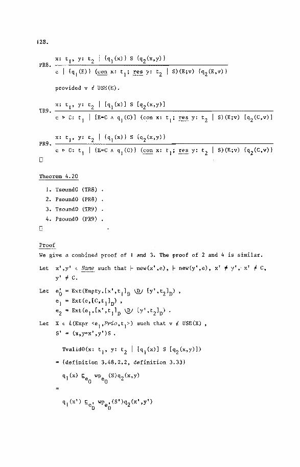
128.
x: t 1, y: t 2 {q1(x)} s {q2(x,y)} PR8.
c I {q1(E)} x: t
1; res y: t 2 I S)(E;v) {q
2(E,v)}
provided v i USE(E).
x: t 1, y: t2
I [q1(x)] s [q
2(x,y)]
TR9. c ~ C: t
1 I [E=C A q
1(c)] (con x: t
1; res y: t
2 I S)(E;v) [q2 (C,v)]
x: t1
, y: t2
I {q1(x)} s {q
2(x,y)}
PR9.
0
Theorem 4.20
1. TsoundO (TR8)
2. PsoundO (PR8)
3. TsoundO (TR9)
4. PsoundO (PR9)
0
Pro of
We a combined proof of I and 3. The proof of 2 and 4 is similar.
Let x' ,y' E Name such that 1- new(x' ,e), 1- new(y• ,e), x' 'I y', x' 'I C,
y' + c.
Let e0 = Ext(Empty,[x',t 1]D ® [y',t2]D),
e1
= Ext(e,[C,t 1]D),
= Ext(el'[x' ,t 1]D \Q/ [y' ,t2]D) •
Let X E L (Expr <e 1 ,Prio, t
1 >) such that v i USE (X) ,
S' = (x,y+x' ,y' )S •
TvalidO(x: t1
, y: t 2 I [q1(x)] S [q
2(x,y)])
{definition 3.48.2.2, definition 3.33}

(I) q1(x') c: wp (S')q (x' y')
-e2
e2
2 '
Consider
wp ((con x: t1
; res y: t 2 I S)(E;v))q2 (X,v) el-
{definitions 4.18.1, 4.17.1}
{x' + E)wp (S'){v + y')q2(X,v) e2
{v i USE(X), lemma 4.7, definition 4.6.10.1}
(x' + E)wp (S')q2(X,y') e2
~e {corollary 3.40.1} 2 (x'+ E)wp (S')(x' =X A q2 (x',y'))
e2 {ASSN(S') n USE(x' =X) = 0, lemma 4.5.5}
(x'+ E){x' =X A wpe (S'}q2(x',y')) 2
~ {(1), theerem 3.42.1} -ez (x'+ E)(x' =X A q 1{x'))
={x' i USE(X), lemma 4.7}
E = x A ql (E)
Under the assumption that
holds, we have proven
from which fellows
(2) 1-D c I> C: tl I (E=X) A q(E}
= wpe ((con x: t 1, res y: t 2 I S)(E;v))q2(X,v) • I
We are still free to choose X, subject to the condition v i USE{X).
Two choices are of interest:
129.

130.
D
a. If we choose X = E, (2) can be simplified to
x: t 1, res y: t 2 'I S)(E;v))q2 (E,v) ,
i.e.
TvalidO(c I [q1(E)J (conx: t1
, resy: t2
I S)(E;v) [q2
(E,v)])
provided v i USE(E), hence TsoundO (TR8).
b. If we choose X = c, v i USE(X) is satisfied, and we obtain from
(2)
~D c. C: tl I (E=C) A 9)(E)
~ wp ((con x: t1
, res y: t2
I S)(E;v))q2(c,v) el-
or equivalently:
~D c. C: tl I (E=C) A qi(C)
i.e.
~ wp ((con x: t 1, res y: el-
Tvalido(c • C: t 1
I S)(E;v))q2(C,v) ,
I [E=C A q1(C)] (con x: t 1, ~ y: t 2 I S)(E;v) [q2(C,v)]) ,
hence TsoundO (TR9).

131.
4.3. Parameterless recursive procedures
4.3.0. Introduetion
The third aspect of the procedure concept we want to study in isolation
is recursion. In order to concentrata on this subject we will temporar
ily- i.e. throughout section 4.3 - ignore other aspects of the
language definition, such as precise syntax, scope rules, nes~ed
declaratións, parameter mechanisms, etc. We stress the point that the
constructs considered in this section are not part of the souree
language. They only serve to study the effect of recursion on the
structure of semantic equations, proof rules, and soundness proofs.
Accordingly, the scope of definitions and theorems concerning these
constructs is limited to section 4.3.
We will study programs of the form
where the constructs pi = Si (i: I ~ i ~ k) are declarations of
parameterleas and possibly recursive procedures. We omit a precise
specification of the syntax of these programs. Suffice it to say that
the narnes pi are elements of Name, that they are mutually different
and also different from variabie names, that they may occur as state
ment in s1, ••• ,sk,s, and that the statements s1, ••• ,sk,s contain
neither blocks nor abstractions. We omit the specification of environ
ments for wp, wlp, C, T, etc.
Insection 4.3.1 wedefine thesemantics of these programs. Insection
4.3.2 we present some proof rules and prove their soundness.
4.3.1. Semantics
It is our intention, roughly speaking, that a statement p. has the l.
same condition transfarmer as the corresponding statementS .• The l
condition transfarmer of a statement should therefore be defined
relatively to a set of procedure declatations. This can be achieved by
means of an extra argument ö for wp and wlp, being a mapping from
procedure names p. to condition transfarmers of the corresponding l.

132.
statements Si. As the procedures may be mutually recursive the o eer
responding to a set of procedure declarations will be determined by
means of fixed point techniques. The intentions just sketched are
captured by definitions 4.21, 4.23/24, 4.26. In their structure these i
definitions much resembie those encountered in denotational semantics;
see e.g. [de Bakker].
4. 21 {ll}
I , 1':. Name + T •
2, is the standard order on 6.
0
4.22
(ö,~;6 ) is a cel.
0
Proof
Immediately by theorem 3.10.2 and theorem 3.36.
0
As already said the definitions of wp and wlp will be extended with an
argument ó E b.. For the statements of the kernel language this argument
is ignored, but it is essential for the procedure statements.
We will denote the extended versions by,wp' and wlp', respectively.
--'-~-"'-'-~-4 .,_2_3 { wp' } The function wp' E L(Stat) + (ll + T) is 1defined by:
I. wp' (abort) o (Àq E c false)
2. wp'(skip)o (Àq E c q)
3. wp' (v :: E)ö (v-<- E)
4. wp' (s 1 ;s2)0 (wp' (S 1 )a) " (wp' (s2)ö)
5. wp'(ifB+ s 1 U ••• U B + S fi)ö: -I n n-
(Àq E c I [V i I l~i~n I B.] A[Ai 1 I l!>hn
6. wp' (do B1 + s1 0 ... D B + s od)o = J.lf • n n-

where F = ( Àf € C + C I O.q e; C I ([\/i I I ~isn I B. ] v q) ~ 1
A [/\i I l::>i::>n IB. • (wp'(S.)o)f q])) 1 1
7. wp'(p)o = o(p) •
0
Definition 4.24 {wlp'}
The function wlp' € L(Stat) + (~ + T) is defined by:
I. wlp'(abort)ö (Àq e; C true)
2. wlp'(skip)ê = (Àq E C q) •
3. wlp'(v := E)ó (v + E) •
4. wlp'(S1;s
2)ó (wlp'(S
1)ó) o (wlp'(S2)ö)
5. wlp'(if B1 + s1 0 ... 0 B + S fi)ê = - n n-
(Àq € c I [/\i I l~i::>n I B. => (wlp' (S.)o)q) ]) • 1 1
6. wlp'(do B1
+ s1
0 ••• DB + S od)o = vG, - n n-
where G = (H E C +de C I (Àq E C I ([V i I l::>i::;n I Bi 1 V q)
7. wlp'(p)ö o(p) •
0
A [/\i I lsisn I Bi=:> (wlp'(Si)ó)f q]))
As with definitions 3.37 and 3.38 in chapter 3, definitions 4.23 and
4.24 above are well-formed only if F and G are continuous, which in
turn depends on continuity of wp' and wlp'. That this is indeed the
case is stated in the following theorem.
Theorem 4.25
I. For all SE L(Stat), ö E Name+ (C + C): uc
wp'(S)ó E C + C uc
133.
If Sis of the form do B1 + s1 D ... 0 Bn +Sn od, and Fis as in
definition 4.23.6, then
F E (C + C) + (C + C) • uc uc uc

134.
0
2. For all S E L(Stat), o E Name+ (C +de C):
wlp'(S)ö E C +deC.
If Sis of the form do B1
+ s1
D ... D Bn +Sn od, and Gis as in
definition 4.24.6, then
G E (C +de C) (C +de C) •
Proof
We only consider 1.
The proof is by induction on the composition of S. Apart from the ö
argument the first six cases are identical to those in the proof of
theorem 3.39.1. Therefore we only consider the case.that Sis a
procedure statement.
0
1.7,S::p
wp' (S)ö
{definition 4.23.7}
o(p)
E {ö E Name+ (C + C)} uc
c... c . uc
Fora program PI = s,, ••. ,pk = sk I s wi will define the condition
transfarmers wp and wlp in terms of wp' and wlp' respectively, where
the argument o E ~ depends on the procedure declaration part.
Definition 4.26 {wp and wlp for p 1 = s1 ,' ••• ,pk
where ö is the function {(pl'<pl), .. ,.,(pk,(!)k)},
((!) 1, ••• ,<pk) = ~(~ 1 , ••• ,~k)' and, fo~ i: 1 ~ i~ k:

0
2. wlp(pl = sl, ••• ,pk = sk I S) = wlp'(S)ö,
where ö is the function {(p 1 ,~ 1 ), ••• ,(pk'~k)},
(~l'''''~k) = v(~ 1 ••••• ~k), and, for i: I $i $ k:
135.
Again, these definitions are well-formed only if the functions ~i and
~. are upward continuous and downward continuous, respectively. This ~
is assured by the following theorem:
Theorem 4.27
For all SE L(Stat):
0
I. (À~J'''''~k E C +uc C I wp'(S){(pl'~l), ••• ,(pk'~k)})
E (C + C)k + (C + C) • ue uc ue
2. (À~ 1 , ••• ,~k E C +deC I wlp'(S){(p 1 ,~ 1 ),.,.,(pk'~k)})
E (C +de C)k +de (C +de C) '
Proof
We only prove I; the proof of 2 is similar when dual versionsof
theorema 3.24 and 3.26 are used.
The proof is by induction on the composition of S. In the scope of
~ 1 , •••• ~k E C +ue C we will write ö for {(p 1 ,~ 1 ), ••• ,(pk'~k)}.
1.1 - 1.3. S :: abort, S :: skip, S :: v := E
By definition 4.23.1-3:
for all ~ 1 , ••• ,~k E C +uc
of , 1, ••• ,~k'
So, by theorem 3.24.1:
C: wp'(S)ö E C + C and independent uc
(À'I''''''k E C +uc C I wp'(S)ö) E (C +uc C)k +ue (C +ue C) •
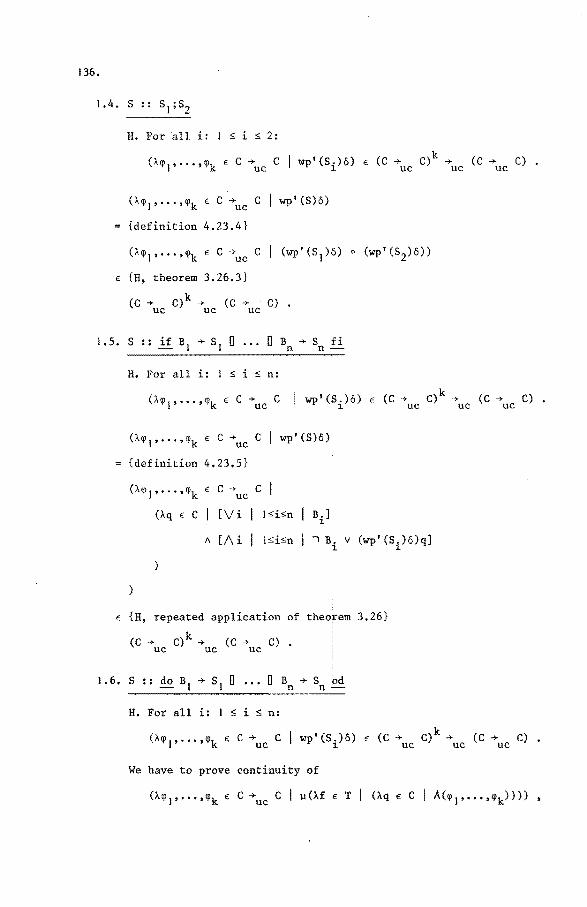
136.
H. Fer ~11 i: I ~ i ~ 2:
(À~~·····~k E c + c I wp'(SJ..)ö) E (C + C)k + (C + C) • uc uc uc uc
(À~)' ••. ,<pk E c ..,.uc c I wp' (S)ö)
{definition 4.23.4}
(À<tJI' ... ,<tJk E c ..,.uc c 1 (wp'Cs 1)ö) o (wp'(s2)o))
E {H, theerem 3.26.3}
(C + C)k ->- (C ->-uc C) uc uc
H. For all i: I ~ i ~ n:
I wp'(S.)ö) E (C + C)k + (C..,. C) • J. uc uc uc
(Àrp) •••.• ~k E C ->- c I wp' (S)ö) uc
{definitien 4.23.5}
(À~, .... ,<pk " c..,. c I uc
(Àq E C [V i l~i~n B.] J.
A [A i l~i~n ï B. v (wp' (S.)ö)q] J. J.
E {H, repeated application of theerem 3.26}
(C + C)k ->- (C + C) • uc uc uc
1.6. s .. B1 ->- s1
U ••• 0 B ->- S od n n-
H. For all i: I ~ i ~ n:
(À<p1
, ••• ,~k E C->- C I wp'(S.)ö) E (C->- C)k->- (C->- C) • uc J. uc uc uc
We have to prove continuity of

0
([Vi
A [ 1\ i
l~i~n B.] V q) l.
l~i~n Bi • (wp'(S){(p 1 ,q~ 1 ), ••• ,(pk,cpk)}) fq]).
Let <~.>~ 0
be an ascending chain in (C + C)k. J J'" uc
137.
(Àcp 1, ... ,cpk EC ... c IJJ<H ET 1 (Àq EC 1 A(QJ 1, ••• ,q;k))))(.Ü0 ~.) uc J'" J
{S-reduction}
]J(Àf E T I (Àq E c A cü0 <P • ) ) ) ) J'" J
~ {H, repeated application of 3.26}
]J(Àf E T I (Àq E c .Ü0 A(~.))) J'" J
= {definition lub}
]J(Àf ET I j~O (Àq E c I A(~j))) = {definition lub}
JJ(.Ü0
<H E T I (Àq E c 1 A(~.)))) J= J
= {continuity ]J, see [de Bakker, theorem 5.11)}
j~O ]J (H E T I (Àq E c I A(~ j)))
= {S-expansion}
j~O (À<pt' ... '<pk E C+ucc I (HET I (t..qEC IA<<p 1, ... ,<pk))))(~j).
1.7. S ::= Pj
(t..cp 1, ••• ,cpk E C +uc C I wp'(S)ö)
{definition 4.23.7}
(À<pl, ••• ,q;k E C +uc C I ó(pj))
{ö = {(pl,cpl), ••• ,(pk,cpk)}}
(À<pl, ••• ,q;k E c ... uc c I q;j)
E {theorem 3.24.2}
(C ..,. C)k ..,. (C _,.uc C) uc uc

138.
As already said it is our intention that a statement pi has the same
condition transfarmer as the corresponding statement Si. That such is
indeed the case is stated in the following theorem.
Theorem 4.28
Let PI = SJ'''''pk = sk I s be a program.
I. Let ó be as in definition 4.26.1.
For all i: I s; i s k: wp' (p.)ö = wp' (S.)ö. ~ ~
2. Let ö be as in definition 4.26.2.
For all i: I s i s k: wlp'(pi)ö = wlp'(Si)ö.
0
Pro of
We only prove 1; the proof of 2 is similar.
Let i: 1 s i s k.
0
wp'(pi)ö
{definition 4.23.7}
ö(pi)
{definition 4.26.1, ö}
<pi
{fixed point propery}
<!>i(<pl'"''<pk)
{definition 4.26.1, <!>i}
wp' (Si)ö •
The following examples illustrate how certain recursive procedures
relate to statements of the kernel language.
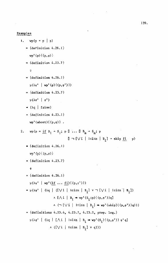
Examples
I. wp(p = p I p)
= {definition 4.26.1}
wp'(p){(p,(j))}
= {definition 4.23.7}
= {definition 4.26.1}
)l(À(j)' I wp' (p){(p,(j)')})
= {definition 4.23.7}
Jl(À{j)' I {j)')
(Àq I false)
{definition 4.23.1}
wp'(abort){(p,(j))} •
2. wp(p = if B1 + s 1; p D ... D Bn +Sn; p
D ï [Vi I l!>i!>n I Bi]+ skip fi I p)
= {definition 4.26.1}
wp'(p){(p,(j))}
= {definition 4.23.7}
= {definition 4.26.1}
(Àq I ([V i l!>i!>n IB.] Vï[Vi I l!>i!>nÎ B.]) L L
11 [/\i B. *wp'(S.;p){(p,(j)')}q] L L
11 (ï[\/i I l!>i!>n IB.] *wp'(skip){(p,q1 1 )}q))) L
{definitions 4.23.4, 4.23.7, 4.23.2, prop. log.}
)l(À(j)' I (Àq I [/\i
" ([\/i
l!>i!>n B. *wp'(S.){(p,q1 1)} q1'q]
L L
l!>i!>n B.] V q))) L
139.
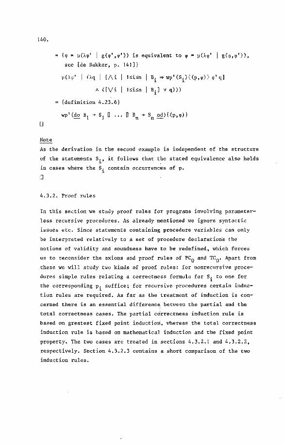
140.
{cp = J.I(Äcp 1 I g(cp' ,qJ')) is equivalent to cp
0
No te
see [de Bakker, p. 141]}
].I(Ä(jl' I Oq I [/\i
A ([Vi
{definition 4.23.6}
lsün
ISisn
B • .,.wp'(S.){(p,cp)} cp 1 q] l 1
B.] V q))) l
As the derivation in the second example is independent of the structure
of the statements Si, it follows that the stated equivalence also holds
in cases where the Si contain occurrences of p.
0
4.3.2. Proof rules
In this sectien we study proof rules for programs invalving parameter
less recursive procedures. As already mentioned we ignore syntactic
issues etc. Since statements containing procedure variables can only
be interpreted relatively to a set of procedure declarations the
notions of validity and soundness have to be redefined, which forces
us to reconsider the axioms and proof rules of PC0 and TC0• Apart from
these we will study two kinds of proof rules: for nonrecursive proce
dures simple rules relating a correctness formula for Si to one for
the corresponding pi suffice; for recursive procedures certain induc
tion rules are required. As far as the treatment of induction is con
cerned there is an essential difference between the partial and the
total correctness cases. The partial correctness induction rule is
based on greatest fixed point induction, whereas the total correctness
induction rule is based on mathematica! induction and the fixed point
property. The two cases are treated in sections 4.3.2.1 and 4.3.2.2,
respectively. Sectien 4.3.2.3 contains a short comparison of the two
induction rul es.

141.
4.3.2.1. Proof rules for partial correctness
In this section we discuss the partial correctness logic for programs
irivolving parameterleas recursive procedures. We begin with defini
tions of validity and soundness.
On "partial correctness formulae" x "procedure declarations" the
predicate Pvalidl is defined as:
IJ
2. Pvalidl(c {q1} S {q
2}, (p 1=s 1, ••• ,pn=Sn)) =
1-D c ql *wlp'(S){(pl,(j.I), ... ,(pn,q,n)} q2'
where ((j. 1, ••• ,(j.n) = v(~ 1 , •••• ~n) and ~ 1 , ••• ,~n are as in defini
tion 4.26.2.
Definition 4.30 {Psoundl}
On "partial correctness proof rules" x "procedure declarations" the
predicate Psoundl is defined as:
Psoundl
D
1 ,.~.,fn, pd) =
l~i~n I Pvalidl(f.,pd)),. Pvalidl(g,pd) • "~
The following theorem statea that the partial correctness logic PC0 of chapter 3 is also sound with respect to these revised definitions:
Theorem 4.31
D
. I. (~a E AxPC: Pvalidl(a, (p 1=Sl''"'Pn"'Sn)))
0
2. (~rE PrPC Psoundl(r, (p 1=s 1, ••• ,pn=Sn))) 0
Proof
Similar to that of theorem 3.52. Details omitted.
D

142.
In addition ro Prpco we need rules to derive properties of procedure
statements. The following theorem states the soundness of a rule for
use with nonrecursive procedures.
Theorem 4.32
(~i I l$i$n I Psoundl (:
0
Pro of
Immediately by definitions 4.29 and 4.30 and by theorem 4.28.2.
0
For recursive procedures this rule is insufficient; some form of
induction is required. In the literature [e.g. Hoare 3, Apt I] an
induction rule of the following form is sometimes used:
It should be noted that the form of this rule is misleading. Actually
it is not a proof rule since its premiss is not a correctness formula
but a meta-statement about the derivability of one correctness formula
from another one by means of the axioms and proof rules of PC0 (see
e.g. [Apt 2] fora discussion). Nevertheless we will adopt the above
form, but we will interpret it as the following theorem.
Theorem 4.33
If c I {ql} p {q2} ~PC c I {ql} s {q2} 0
then Pvalidl(c I {q1
} p {q2
}, p = S) •
0
No te
For simplicity we restriet ourselves to a single procedure. The results
can easily be extended to programs with more procedures.
0
143.
The proof of this theorem requires some extra provisions. The conclu
sion of the theorem is based on the interpretation of the condition
transfarmer of p as v~, viz. ~D c I q1
• (v~)q2 • In order to prove
this result by greatest fixed point induction we have to show that
If we want to derive this from the premiss of the theorem it follows
that we also have to consider soundness of PC0 with respect to other
interpretations 4. Therefore, in order to prove theorem 4.33 we first
introduce different notions os validity and soundness and we show that
PC0 is sound in terms of these notions as well.
Definition 4.34 {Pvalid2}
On "partial correctness formulae" x (C +de C) the predicate Pvalid2 is
defined as:
1. Pvalid2 (c
2. Pvalid2(c
0
Definition 4.35 {Psound2}
On "partial correctness proof rules" x (C +de C) the predicate Psound2
is defined as:
Psound2 (fl'·~·,fn, 4) =
(A i I l~i~n I Pvalid2(f.,4)) • Pvalid2(g,4) • - ~
0
Theorem 4 36
0
I. (!a E AxPC, 4 E C +deC: Pvalid2(a,4)) • 0
2. (! r E PrPC , 4 E C +de C: Psound2{r,4)) 0
Proof
Similar to that of theorem 3.52. Details omitted.
0

144.
Definitions 4.34 and 4.35 and theor~m 4.36 enable us to prove theorem
4.33:
Proof of theorem 4.33
.,. { theorem 4. 36}
(!::_ $ I Pvalid2(c
{definition 4.34}
{definition 4.23.7, definition 4.26.2, ~}
q, I (f-D c I ql ... <J,q2) .. (f-D c I ql .. '1'(1f)q2))
{f-D c I q1 .,. (Àq I true)q2, g.f.p. induction, admissibility is trivial}
1-D c I ql .,. (v'l')q2
{definition 4.29}
Pvalidl(c I {q1} p {q2J, p = S)
0
4.3.2.2. Proof rules for total correctness
The structure of this section parallels that of 4.3.2.1. We begin with
definitions of validity and soundness relative to a set of parameter
leas recursive procedures:
Definition 4.37 {Tvalidl}
On "total correctness formulae" x "procedure declarations" the predi
cate Tvalidl is defined as:

2. Tvalidl(c [q 1] S [q2], (p 1=s 1, ••• ,pn=Sn)) =
~D c ql •wp'(S){(pl'~l), ••• ,(pn'~n)}q2
145.
where (~ 1 , ••• ,~n) = ~(~ 1 , •••• ~n) and ~ 1 , ••• ,~n are as in defini
tion 4.26.1.
0
Definition 4.38 {Tsoundl}
On "total correctness proof rules" x "procedure declarations" the
predicate Tsoundl is defined as:
0
Tsoundl (f 1 ,.~.,fn, pd) =
(!:_ i I l:Si:Sn I Tvalidl (f. ,pd)) • Tvalidl (g,pd) • l.
The following theorem states that the total correctness logic TC0 of
chapter 3 is also sound with respect to these revised definitions:
Theorem 4.39
I, (!:_a E AxTC Tvalidl(a, (p 1=s 1, ... ,pn=Sn))) • 0
2. (!:_rE PrTC Tsoundl(r, (p1=s1, ••• ,pn=Sn))) 0
0
Similar to that of theorem 3.54. Details omitted.
0
For nonrecursive procedures we have the following analogue of theorem
4.32:
Theorem 4.40
(A i I I:Si:Sn I Tsoundl (:
0
[ql] 8i [q2J ' (pi'"8 I'''''Pn'"8n)l)
[qiJ Pi [qz] )

146.
Pro of
Immediately by definitions 4.37 and 4.38 and by theerem 4.28.1,
D
Again we need an induction rule to deal with recursive procedures,
The induction principle employed differs from that in sectien 4.3.2.1
however. There we had to use fixed point induction and to extend the
notions of validity and soundness. Here ordinary mathematica! induction
is sufficient to prove the following theorem.
Theerem 4.41
Let <q.>~ 0 be a sequence of conditions. ~ ~=
If (~ i I Osi I c I [[V j I thenTvalidl(c I [[Vi I Osi I 0
OSj<i I q.]] p [r] J ~TC
0 c I [q.] S [r])
~
q.]] p [r], p = S) , ~
No te
As insection 4.3.2.1, we have restricted ourselves to programs with a
single procedure.
0
Proof
(~ i I Os i I c I [ [V j I Osj <i I q.] J p [ r] J
~TCo
c I [q. 1 S [r] ~
• {theorem 4.39}
(~i I Osi I Tvalidl (c I [[V j I 0Sj<i I q.]J p [r], p = S) J
Tvalidl(c I [q.] S [r], p S) ~
{definitions 4.37, 3.33, ~ and ~as in definition 4.26.1}

147.
(!,i I os;i I [Vj I Os;j <i I q. J J
!;;; <pr
.. qi !:: ~(q>)r
)
{<p ~(<p)}
(!,i I O::>i [Vj I O::>j <i I qj J ~ <pr .. q. ~
!:. <pr
,. {lemma 3.29}
[Vi I 0Si I q.] !:. q>r ~
{definitions 4.37, 3.33, <p}
Tvalidl(c I [[Vi I Osi I q.]] p [r], p = S) • ~
0
From theorem 4.41 a total correctness induction rule can easily be
derived. If we define qi as q A e = I, where e is an integer expression
and I a symbol sequenèe representing i, we obtáin that
[V j
and [Vi
OSj<i I q.] = q A 0 s e A e < I , J
Osi I q.] = q A 0 ::> e ·• ~
In this case the theorem reduces to:
If (!, i I OSi I c I [q A 0 ::> e A e < I] p [r]
I-Tc0 c I [q A 0 s e A e = I] S [r]
then Tvalidl (c I [q A 0 s e] p [r] )
which we will write, in analogy to the partial correctness induction
rule, as

148.
c I [~ A 0 ~ e A e < I] p [r] ~TC c [q A 0 ~ e A e 0
c I [ q A 0 ~ e] p [ r]
I] S [ r]
4.3.2.3. A noteon the induction rules and their proofs
It may seem strange that the induction rules for partial and total
correctness, which look so much alike, require rather different proofs.
In this section we summarize the structure of these proofs, so as to
clarify the differences. In fact, these differences were already
present in the proof rules PR4 and TR4 for the DO-construct given in
chapter 3, which were basedon theorems 3.46.2 and 3.47.2, respectively.
In theorems 4.33 and 4. 11, however, the differences are much more pro
nounced. Let us reconsider the structure of their proofs.
The proof of theorem 4.33, the partial correctness case, is essentially
of the following form:
Let q1
and q2 be two conditions.
Let ~ be as in definition 4.26.2.
From the premiss and the extended soundness notion it follows
that for all q,: (p ç !J>q) ,. (p ç ~(q,)q).
As the base step and admissibility are trivially satisfied, it
follows by greatest fixed point induction that p ç (v~)q.
The proof of theorem 4.41, the total correctness case, is essentially
of the following form: co
Let <qi>i=O be a sequence of conditions
Let r be a condition.
Let~ be as in definition 4.26.1, and let~ ~~.
premiss
• (for all i: 0 ~ i: (0 LJ • q. c cpr),. (q~ ç Hcp)r)) ~J<l. J - ~
• {fixed point property: cp = ~(cp)}
(for all i: 0 ~ i: (0<w<. q. c q.t).., (q. ç ~r)) -J l. J - l.
{lemma 3.29}

149.
Note that in the latter proof it is not necessary that w is the least
fixed point of ~; only use has been made of the fixed point property
w - ~(~).
150.
4.4. Recursive procedures with parameters
4.4.0. Introduetion
In this section we will study programs of the form
where the pi are identifiers, the Ai are abstractions, and B is a
block. The constructs pi = Ai are to be considered as procedure
declarations. Within the abstractions A. and the block B statements l.
may occur of the form p.(EL;VL), where EL is a list of expressions and J
VL is a list of variables with types and lengths that match those of
the abstraction A. corresponding J
in such a way that the statement
top .• Thesemantics will be defined J
p.(EL;VL) is equivalent to the stateJ
ment A.(EL;VL), even if p. has been defined recursively. J J
The treatment of this subject is essentially a combination of the
treatments of parameterization and recursion in sections 4.2 and 4.3,
respectively. In fact (and intentionally} there is so much correspon
dence that in many places we have taken the liberty to replace (parts
of) definitions and proofs by an appeal to the similarity to their
counterparts in those sections. Insection 4.4.1 we deal with the
syntactic aspects, in 4.4.2 with the semantics and in 4.4.3 with the
proof rules.
4.4.1. Syntax
Apart from some additional production rules the main syntactic exten
sion is the introduetion of a new attribute domain Penv to establish
the correspondence between declaration and use of procedure identi
fiers. The role of Penv-attributes is comparable to that of Env
attributes. It would have been possible to combine the two, but for
the sake of clarity we have refrained from doing so. Below we give
the extensions, followed by some informal explanation.
Domains
Penv

OEerations on Penv
[. . . ] ' ' 'P
Name *Types *Types + Penv . w . Penv * Penv + Penv 11 p (·,·) Name * Penv + Int
(·,•,•) .. Name * Types * Types * Penv + Bool
liP (n 1,[n2,ts 1,ts2]:P) = if n 1 • n2 +I D n1 {< n2 + 0 fi
liP (n,pe 1 \Jl'pe2) = #P (n,pe 1) + liP (n,pe2)
(n1,ts 1,ts2) inp [n2,ts3,ts4lp
(n,ts 1,ts2) inp pe 1 \El pe2
(n1 = n2 A ts 1 ts3 A ts2 = ((n,ts 1,ts2) inp pe 1) v
((n,ts 1,ts2) inp pe2)
Nonterminals
Procdecs <Penv,Penv>, Abstr <Penv,Types,Types>, Block <Penv,Env>,
Stat <Penv,Env>, Gcs <Penv,Env>.
{see note below}
Grammar rules
Prog
pel • pe2
(~ n: Name
e = Empty
Block <pe 1 ,e> •
Procdecs <pe0 ,pe 1> ::= Id <n> = Abstr <pe0,ts 1,ts2> •
pe 1 = [n,ts 1,ts2JP
con Pdecs <d 1,ts 1>
res Pdecs <d2,ts2>
Stat <pe,e>
) . n: Name I #D (n,d 1 @d2) + #p (n,pe) ~ I)
e = Ext(Empty,d 11Wd2)
151.

152.
Stat <pe,e>
Explanation
::= Id <n> (Exprs <e,ts1>
Vars <e,ns,ts2> ) •
(!:_ n: Name I #N (n,ns) ::::: I)
(n,ts 1 ,ts2 ) iEp pe
The Penv-attributes establish the correspondence between procedure
narnes and the parameter types of the corresponding abstractions. With
the nonterminal Procdecs two such attributes are associated. The first
one records information about all procedures declared in the procedure
deelaratien part of a program; it is used to describe the legitimacy
of procedure applications. The second one contains information con
cerning the internal procedure declarations. At the outermost level
these attributes must be equal. The rules for formal-actual parameter
correspondence are the sameasin sectien 4.2.1. Abstractions have no
access to global variables. Narnes of formal parameters must differ
from procedure names (see also note I below).
D
No te
A Penv-attribute bas also been associated with the nonterminals Block,
Stat, and Gcs. Strictly speaking we should give new versions of the
grammar rules for these nonterminals, However, as in most of these
rules the Penv-attribute is merely, "passed on", as e.g. in
Stat <pe,e> ::=Stat <pe,e>; Stat <pe,e> •
we will not list them anew. The only exception is the rule for Block,
which obtains the additional rule condition that variabie narnes must
differ from procedure names:
D
Block <pe,e0> ::= I[ var Decs <d> I Stat <pe,e1> ]I •
(!:_ n: Name I #D (n,d) + #P (n,pe) s I)
e 1 • Ext(e0 ,d)

153.
No te
As insection 4.2.1, an additional context condition is formulated by
means of the functions USE, ASSN, and INIT. This part is almost
identical to definitions 4.13 and 4.14 and the context condition
following them, and therefore it is not repeated here.
0
4.4.2. Semantics
In this section we define the semantics of programs of the form
PI = Ap .. ••Pk = ~ I B. Basically this definition has the same struc-
ture as that insection 4.3.1, the main difference being that with
each name pi a parameterized condition transformer rather than a
condition transfarmer has to be associated. Similarly to section 4.3.1,
these associations are established by means of an argument ö added to
wp, wlp, pwp, and pwlp. Omitting environments for a while, the central
clauses of the new definitions are:
wp'(p(E;v))ö ~ pwp'(p)ö(E,v)
and pwp'(p}ö • ö(p} •
The ö corresponding to a procedure deelaratien part is determined by
means of fixed point methods.
An essential complication is that procedure applications may occur in
different contexts. We reeall definition 4.15, which defines P as the e
set of parameterized condition transfermers corresponding to an envi-
ronment e E Env. It follows that ö has to be parameterized with regard
to the environment e of the procedure application, so as to obtain the
appropriate element of Pe. Hence ó € + Env + U P in such a eEEnv e' way that for all procedure names p and e € Env: o (p) (ë)-E P •
--- . e
Apart from the points just mentioned, the definitions given in this
sectionare very similar to those in sections 4.2.2 and 4.3.1, so we
abstain from further clarification. The definitions follow.
Definition' 4.42 {X}
0
X= {~ E Env + U Pe eEEnv

154.
Definition 4.43 {ç_x}
For all <pl,<p2 E X:
q>l !;:x q>2 fif
0
Theorem 4.44
(X,~X) is a cel.
0
Pro of
(~ e E Env I <pi (e) !:.p QJ2 (e)) . e
That ~X is a partial order follows immediately from definition 4.43,
theorem 4.15 and theorem 3.10.2.
Let Y be a countable subset of X.
u y {;\e E Env ~~ cp(e))
q>EY
n Y (Xe E !Pel q>(e))
QJEY
0
Definition 4.45 {6}
6 =Name +X
Definition 4.46 {wp'}
For all e E Env the function wp~ E L(Stat <Penv,e>) + 6 +
by:
1-6. Similar to definition 4.23.1-6.
7. wp~(A(E;v))o = pwp~(A)(o)(E,v)
8. wp~(p(E;v))o pwp~(p)(o)(E,v)
0
Definition 4.47 {wlp'}
is defined
For all e E Env the function wlp~ E L(Stat <Penv,e>) + 6 +Te is
defined by:
1-6. Similar to definition 4.24.1-6.

7. wlp~(A(E;v))ö = pwlp~(A)(o)(E,v).
8. wlp'(p(E;v))o = pwlp'(p)(o)(E,v) • e e D
Definition 4.48 {pwp', pwlp'}
For all e E Env the functions pwp~ and pwlp~ E L(Id <Name>)
u L(Abstr <Penv,Types,Types>) + 8 + P are defined as fellows: e
Let (~x: t 1;!!! y: t2
I S) E L(Abstr <Penv,Types,Types>),
E, V, x', y', e', S' as in definition 4.17.
D
J.J. pwp~((~ x: t 1; res y: t 2 I S))O =
(ÀE E E, v E V I (x'+ E) o wp~,(S')o o (v + y')) •
1.2. pwp~(p)ö = o(p)(e) •
2.1. pwlp~((con x: t 1; res y: t 2 I S))o =
(ÀE E E, v.;: V I (x'+ E) o wlp~,(S')o o (v + y'}) •
2.2. pwlp'(p}o = o(p)(e) e
No te
Continuity of the functions defined above can be proven similarly to
theerem 4.25. Details omitted.
D
Definition 4.49 {wp and wlp for programs}
where e0 = Empty,
ó is the function {(p 1 ,~ 1 ), ••• ,(pk'~k)}, (~J'''''~k) = ~(~J'''''~k)' and, for i: I s i s k:
where e0 = Empty,
wlp' (B)ö , eo
155.

156.
0
No te
6 is the function {(p 1 ,~ 1 ), ••• ,(pk'~)},
(q,,, ••. ,q,k) =\i('!' I' ... ,'l'k)'
and, for i: I $ i $ k:
Continuity of the functions ~i and 'l'i can be proven similarly to
theorem 4.27. Details omitted.
D
The following analogue of theorem 4.28 states the equivalence of the
statements pi(E;v) and Ai(E;v) when pi= Ai is a procedure declaration.
Theorem 4.50
Let
IJ
e " Env, i: $Î$;k,
E, v such that A.(E;v) "L(Stat <Penv,e>). l
I. Let 6 be as in definition 4.49.1.
wp 1 (p.(E;v))6 = wp'(A.(E;v))6. e 1 e 1
2. Let 6 be as in definition 4.49.2.
Pro of
We only prove I; the proof of 2 is similar.
wp' (p. (E;v))6 e 1
{definition 4.46.8}
pwp~(pi)(6)(E,v)
{definition 4.48.1.2}
6(pi)(e)(E,v)
{definition 4.49.1, 6}

D
<pi (e) (E,v)
{fixed point property}
Wi(<p 1, ••• ,<pk)(e)(E,v)
{definition 4.49.1, ~.} l
pwp 1 (A.)(ö)(E,v) e 1
{definition 4.46.7}
wp'(A.(E;v))o. e l.
4.4.3. Proof rules
4.4.3. I. Proof rules for partial correctness
157.
In this section we discuss partial correctness proof rules for programs
of the form p1 = A1, •.. ,pk = ~ I B. The structure of this section
resembles that of section 4.3.2.1. First wedefine validity and sound
ness relatively to a set of procedure declarations, and we prove sound
ness of a rule to be used with nonrecursive procedures. Thereafter we
consider an induction rule for use with recursive procedures. As in
section 4.3.2.1, the proof of the latter rule requires definitions of
validity and soundness relatively to an arbitrary interpretation ~ for
procedure names.
Definition 4.51 {Pvalid3}
On "partial correctness formulae" x "procedure declarations" the
predicate Pvalid3 is defined as:
D
I. Pvalid3(c q, (p 1=A1, ••• ,pk=~ I B)) = ~D c I q.
2. Pvalid3(c {q1} S {q2}, (p1=A1, •.• ,pk=~ I B)) =
~D c q1 • wlp~(S)(ö)(q2 ) ,
where c ~ L(Cont <e>), q1,q2 E L(Cond <e>), and ö is as in defini
tion 4.49.2.

158.
Definition 4.52 {Psound3}
On "partial correctness proof rules" x "procedure declarations" the
predicate Psound3 is defined as:
(~ i I 05i5n I Pvalid3(c0 I fi' pd)) ~ Pvalid3(c 1 I fn, pd) .
0
It is easy to prove that the axioms and proof rules considered in
sections 3.3, 4.1.4, and 4.2.3 are valid c.q. sound" in termsof these
extended notions as well. For easier reference we collect these axioms
and rules under the name PC 1:
Definition 4.53 {PC1}
The partial correctness logic PC 1 is defined by:
0
PrPC u {PR5,PR6,PR7,PR8,PR9} • 0
Theorem 4.54
0
I. (~a tt:. AxPC 1
2. (~ r € PrPC I
Pro of
Similar to those of theorems 3.52, 4.12, and 4.20. Details omitted.
0
Below, for simplicity we restriet ourselves to the case k: I. The
results can easily be extended to progriams with more procedure declara
tions. First, we present proof rules for use with nonrecursive proce
dures.

Definition 4.55 {PRlO, PRil}
Let A= (~x: t 1; ~ y: t 2 I S) ~ L(Abstr <Penv,Types,Types>),
Let E, v, c, C, q1, q2 be as in definition 4.19.
The proof rulesPRIO and PRil are defined by:
PRIO x: tl' y: t 2 I {q1(x)} s {q2(x,y)}
c I {q1(E)} p(E;v) {q2(E,v)}
provided v t USE(E).
PRIJ. x: t 1, y: t 2 I {q1(x)} S {q2(x,y)}
ct> C: t 1 I {E-C A q1(c)} p(E;v) {q2(c,v)}
0
Theorem 4. 56
0
l, Psound3(PRIO, p =A)
2. Psound3(PR11, p =A) ,
Proof
We only consider I; 2 is similar.
Assume:
Pvalid3(x: t 1, y: t 2 I {q1(x)} S {q2(x,y)}, p =A).
By a proof almost identical to that of theorem 4.20 we obtain:
Pvalid3(c I {q 1(E)} A(E;v) {q2(E,v)}, p =A)
provided v I USE(E) .
Hence, by definition 4.51 and theorem 4.50.2:
0
Pvalid3(c I {q1(E)} p(E;v) {q2(E,v)}, p =A)
provided v I USE(E) •
159.
Let us now turn to the induction rule for recursive procedures. The
treat~ent of this rule is similar to that of the parameterless induc
tion rule insection 4.3.2.1. First wedefine validity and soundness

160.
with regard to an arbitrary interpretation 4 for procedure names. By
means of these notions we prove theorem 4.61, which is finally
presented as inductive proof rule PR12 •
Definition 4.57 {Pvalid4}
On "partial correctness formulae" x X the predicate Pvalid4 is defined
as:
1. Pvalid4 (c q, q,) = f-D c I q
2. Pvalid4(c { q I } S { q2 } ' <!>)
~D c q1 ~ wlp~(S){(p,q,)}q2 ,
where c E L(Cont <e>), q 1,q2 E L(Cond <e>) .
D
On "partial correctness proof rules" x X the predicate Psound4 is
defined as:
0
D
(A i I 0$i$n I Pvalid4 (c0 I f., q,)) ~ Pvalid4 (c 1 I f , q,) • - 1 n
60
I. (!a E AxPC , q, EX Pvalid4(a,q,)) I
2. (! r E PrPC , q, E X Psound4(r,q,)) • 1
Proof
Similar to those of theorems 3.52, 4.12, and 4.20. Details omitted.
0
Theorem 4.61
Let A= (con x: t1
; res v: t2
l S) E L(Abstr <Penv,Types,Types>).
Let e' = Ext(Empty,[x,t 110 \!ll [v,t2J0),
q1(x),q
2(x,y) E L(Cond <e'>) •
For i: ~ ~ i ~ n:
let ei E Env ,
If
then
D
Pro of
ei E L(Cont <ei>) ,
Ei E L(Expr <epl'l"io,t 1>) ,
vi E L(Var <ei,Name,t2>) , vi
~PC I
i USE(E.) • l.
161.
The proof is by greatest fixed point induction. In the proof we use a
kind of "phase shift" in that we prove validity of correctness formulae
invalving S rather than p(E;v) for arbitrary E and v. This phase shift
leads to shorter formulae. The property we want to prove is:
where ~ is as in definition 4.49.2.
base step
theorem 4.44
• Tx = (Àe E Env I rp ) e
• {definitions 4.47.8, 4.48.2.2}

162.
(A i I J";i:>u I wlp' (p(E.;v.)){(p,T )} (Àq I true)) - e. 1. 1. x
l.
• {definition 4.57}
(A i I I~i~n I Pvalid4(c. I {q 1(E.)} p(E.;v.) {q2(E.,v.)}, TX)) - l. l. l. l. l. l.
• {premiss, theerem 4.60}
induction step
Let (jJ E X.
Pvalid4(x: t 1; y: t 2 I {q 1 (x)} S {q2(x,y)}, (j!)
• {theorem 4.60.2, hence Psound4 (PR8)}
(A i I J";i";n I Pvalid4(c. I {q 1(E.)} A(E.;v.) {q2(E1.,v
1.)}, (j!))
- l. l. l. l.
{definition 4.57}
(! i I I ~i";n I
f-0 c1• I q1(E
1.) •pwlp' (A.){(p,(j!)}(E.,v.)q2(E.,v.) e. l. l. l. l. l.
l.
{definition 4.49.2, o/}
(A i I J";i";n I f-0 c. I q1(E.) •'l'((j!)(e)(E.,v.)q2(E.,v.)) - l. l. l. l. l. l.
{definitions 4.47.8, 4.48.2.2}
<! i I J";i";n I f- 0 c
1• I q(E.) • wlp' (p(E.;v.)){(p,o/((j!))}q2(E.,v.)
l. e. l. l. l. l. l.
{definition 4.57}
• {premiss, theerem 4.60}
As admissibility is trivial, it fellows by greatest fixed point induc
tion that

D
Pvalid4(x: t 1; y: t 2 I {q1(x)} S {q2(x,y)}, v'l')
{definitions 4.57.2, 4.51.2}
Pvalid3(x: t 1; y: t 2 I {q1(x)} S {q2(x,y)}, p =A)
• {theorem 4.56.1}
Finally, in analogy with the parameterleas case in theorem 4.33, we
formulate theorem 4.61 as an inductive proof rule:
PRI2.
I-pc I
c I {q1
(E )} p(E ;v) {q2(E ,v )} n n n n n n
4.4.3.2. Proof rules for total correctness
163.
In this section we discuss total correctness proof rules for programs
of the form p1 = A1, ••• ,pk =~I B. As this section has much in
common with sections 4.3.2.2 and 4.4.3.1, we will shorten the presen
tation somewhat. The main theorem of this section is theorem 4.68, the
induction rule for recursive procedures, also formulated as proof rule
TR12. The structure of the proof is essentially the same as that of
theorem 4.41, the parameterleas induction rule.
Definition 4.62 {Tvalid2}
Similar to definitions 4.37 and 4.51.
D
Definition 4.63 {Tsound2}
Similar to definitions 4.38 and 4.52.
D
164.
Definition 4.64 {TC 1}
The total correctness logic TC 1 is defined by
AxTC = AxTC ' I 0
PrTC u {TR5,TR6,TR7,TR8,TR9} • 0
D
Theorem 4.65
I. (!a € AxTC Tvalid2(a, (p 1=A 1, ••• ,pk=~)) ._ I
2. (! r € PrTC Tsound2(r, (p 1=A1, ••• ,pk=~)) I
0
Proof
Similar to those of theorems 3.54, 4.12, and 4.20. Details omitted.
D
Definition 4.66 {TRIO, TRil}
Let A = (con x: tl; res y: t2 I S) E L(Abstr <Penv,Types,Types>).
Let E, V' c, c, q), q2 be as in definition 4.19.
The proof rules TRJO and TRil
TRIO. x: t 1, y: t2 [ql(x)]
c I [ql(E)]
provided v i USE(E) •
TRI I. x: t), y:
c I> C: tl
0
Theorem 4.67
I. Tsound2 (TRIO, p =A)
2. Tsound2 (TRil, p =A)
0
Proof
are defined by:
S [q2(x,y)]
p(E;v) [q2(E,v)]
Similar to that of theorem 4.56. Details omitted.
0

Theorem 4.68
Let A= (con x: t 1; ~ y: t 2 I S) E L(Abstr <Penv,Types,Types>).
For i: 0 ~i~ n: let ei, ei' Ei' vi be as in theorem 4.61.
Let <q.(x)>~ 0 be a sequence of conditions in J J=
L(Cond <Ext(Empty,[x,t 1]D)>).
Let r(x,y) E L(Cond <Ext(Empty,[x,t 1]D© [y,t2]D)>).
If
<~ k o~ I
~TC I
c 1 I [[\Ij
c I r rv j n
O~j<k
O~j<k q.(E )]] p(E ;v) [r(E ,v )] J n n n n n
x: t 1, y: t 2 I [qk(x)] s [r(x,y)]
then
D
Proof
Let k: k ~ 0.
165.
Tvalid2(x: t 1, y: t 2 I [[\Ij I O~j<k I qj(x)]] S [r(x,y)], p=A)
~ {theorem 4.67.1}
<~ i I 1~i~n I
Tvalid2(c1• I [[Vj I O~j<k I q.(E.)]] p(E
1·;v.) [r(E.,v.)], p =A)
J l l l l
~ {premiss of theorem, theorem 4.65}
Tvalid2(x: t 1, y: t 2 [qk(x)] S [r(x,y)], p =A)
By definitions 4.62, 3.33 and lemma 3.29 it follows that
Tvalid2(x: t 1, y: t 2 I [[\Ik I O~k I qk(x)]] S [r(x,y)], p =A) ,

166.
hence, by theerem 4.67.1,
0
Just as in sectien 4.3.2.2, if we choose qk(x) = (q(x) A h(x) K),
where K is a symbol sequence representing k and h(x) is an integer
expression in terms of x, we obtain that
[Vj O~j<k I q.(E.)] = q(E.) A 0 ~ h(E.) < K J l- l- l-
and [Vk O~k 1 qk(E0)] = q(E0) A o ~'h(E0 ) ,
as a result of which the theorem can be formulated as the following
inductive proof rule:
TRI2.
~TC , I
c1
I [q(E1) A 0 ~ h(E
1) < K] p(E
1;v
1) [r(Epv
1)]
I
c I [q(E ) A 0 s h(E ) < K] p(E ;v ) [r(E ,v )] n n n nn nn
x: t 1, y: t 2 I [q(x) A h(x) = K] S [r(x,y)]

167.
CHAPTER 5
SOME ASPECTS OF THE DEFINITION OF THE TARGET LANGUAGE
S.O. Introduetion
In this chapter we will consider some aspects of the formal definition
of the target language TL. TL has a rather conventional structure; it
contains instructions for loading and storing values, arithmetical
operations, jumps, conditional jumps, subroutine calls and returns.
Usually the effect of these instructions is described operationally in
terms of manipulations with some registers and an instructien pointer.
For our purposes we would like to have at our disposal a condition
transformer definition of TL however. Such a definition will allow us
to derive a mapping from SL to TL from relations between condition
transfermers of SL- and TL-programs.
For simple load and store instructions and the like it is easy to
construct condition transfermers based on that of the assignment. The
difficulties are in the definition of the sequencing instructions. It
is this aspect that we would like to consider in the current chapter.
We shall develop condition transfermers and show their equivalence with
an operational characterization. Rather than presenting two definitions
and proving their equivalence however, we shall derive the operational
description from the condition transformers. This derivation will
proceed via some intermediate versions in which more and more opera
tional aspects are introduced. This chapter therefore has the following
structure.
Insection 5.1 we present an informal description of TL instructions.
In section 5.2 we develop version I of their condition transformer
semantics, which bears some relation to that of parameterless proce
dures in sectien 4.3 and to the continuations of denotational seman
tics. In sectien 5.3 we derive from version I a secoud version, which
is based upon the representation of a TL program as an array of in
structions. In section 5.4 this version is further transformed to

168.
version 3, which employs stacks of return addresses to describe the
subroutine call and return mechanism. Finally, in section 5.5 we
derive from version 3 an operational characterization by means of an
interpreting program. This interpreter is constructed in such a way
that it has the same condtion transformer as that of the TL program in
version 3, and consequently as that in version I.
In some derivation steps use is made of the fixed point property in
order to establish some relation between two versions. Those deriva
tions are given in such a way that it is clear how a full fixed point
induction proof of the equivalence of the two versions should be given.

169.
5.1. Informal description of TL
For the purposes of this chapter, TL may be thought of as consisti· ry
of two sets of variables and of a set of instructions. The variabl~~
of the first set, called the datà variables, are used to repreaent ~:ne
values operated upon by TL programs. For our discussion the properties
of these variables are not very important. For simplicity, let us
assume that the set consists of
M
A and B
Q
the store, a linear array of values,
two general purpose registers,
a condition register.
The second set of variables, the control variables, is mainly used for
sequencing purposes. It consists of
p the program store, a linear array of instructions,
ip the instruction pointer,
rs the stack of return points,
la a function that maps labels to addresses.
A TL program is a construct of the form
where the li are labels and the si are instruction sequences. We dis
tinguish two sorts of instructions, regular and singtilar instructions.
An instruction is regular if the instruction to be executed after its
completion is its textual successor; an instruction is singular, if it
explicitly alters the flow of control, as is the case with jumps, sub
routine calls and returns.
Typically, the effect of regular instructions can be described by
means of a few assignments to the data variables; e.g.:
LDA(a) A := M(a}
STB(a) M(a) := B
ADD(A, B) A := A+ B
GEQ Q := A;;:: B
The description of singular i~structions is less easy. Their formal
characterization is the main subject of this chapter, Here we content
ourselves with a short description in words.

170.
UJP(l)
FJP(l)
TJP(l)
CSR(l)
RET
jump unconditionally to label 1,
if Q is false jump to label 1,
if Q is true jump to label 1,
record return point, jump to label 1,
remove last return point r from record;
jump to r.
We shall assume that programs are closed, i.e. that each label occur
ring in a singular instruction of a program 10 : s0 ; ••• ; 1 1
: s 1
; 1 : n- n- n is an element of {10 , ••• ,ln}.

171.
5.2. Version I: Condition tránsformer semantica of TL
In this section we shall develop condition transfarmer semantica for
closed TL programs. As we are mainly interested in control flow aspects,
we shall restriet ourselves to the singular instructions and to the
regular instructien LDA(a), which serves as representative for all
regular instructions. Throughout the remainder of this chapter (except
for an example) we shall base our discussion on a given closed program
consisting of these instructions only.
Definition 5.1 {Instruction}
Instructien = {LDA(a),UJP(l},FJP(l),TJP(l),CSR(l),RET}
0
Definition 5.2 {Label}
0
We assume as given a cel (C,Ec) of conditions in terms of the
variables of TL.
Definition 5.3 {T,~T}
I. T = C + C. uc
2. is the standard order on T.
0
Letllllla 5.4
(T,~T) is a uccl.
0
lllllllediately by theorem 3.23.2.
0
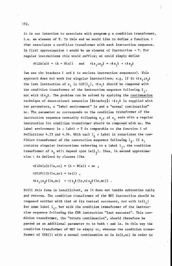
172.
It is our intention to associate with program p a condition transformer,
i.e. an element of T. To this end we would like to define a function T
that associates a condition transformer with each instructien sequence.
In first approximation T would be an element of Instructien + T. For
regular instructions this would suffice; we could simply define
T[ LDA(a)] (A+ M(a)) and
(we use the brackets [ and toenclose instructien sequences). This
approach does not work for singular instructions; e.g. if in T[s 1 ;s 2J
the last instructien of s1
is UJP(li), Tls 1J should be composed with
the condition transformer of the instructien sequence following li'
not with <ls2J. The problem can be solved by applying the continuatien
technique of denotational semantics [Strachey]: Tls1J is supplied with
two parameters, a "label environment" le and a "normal continuation"
nc. The parameter nc corresponds to the condition transformer of the
instructien sequence textually following s 1; if s 1 ends with a regular
instructien its condition transformer should be composed with nc. The
label environment le E Label + T is comparable to the function ö of
definitions 4.23 and 4.24. With each 1'. e Label it associates the con-l.
dition transformer of the instructien sequence following li. lf s 1 contains singular instructions referring toa label 1., the condition
J transformer of s
1 will depend upon le(lj). Thus, in secend approxima-
tion < is defined by clauses like
T[ LDA(a)J (le,nc)
<I UJP(l)D (le,nc)
(A+ M(a)) o nc ,
le(l) ,
Still this form is insufficient, as it does not handle subroutine calls
and returns. The condition transformer of the RET instructien should be
composed neither with that of its textual successor, nor with le(li)
for some label li, but with the condition transformer of the instruc
tien sequence following the CSR instructien "last executed". This con
dition transformer, the "return continuation", should therefore be
passed as an additional parameter re to both T and le. In this way the
condition transformer of RET is simply re, whereas the condition trans
fermer of CSR(l) with a normal continuatien nc is le(l,nc) in order to
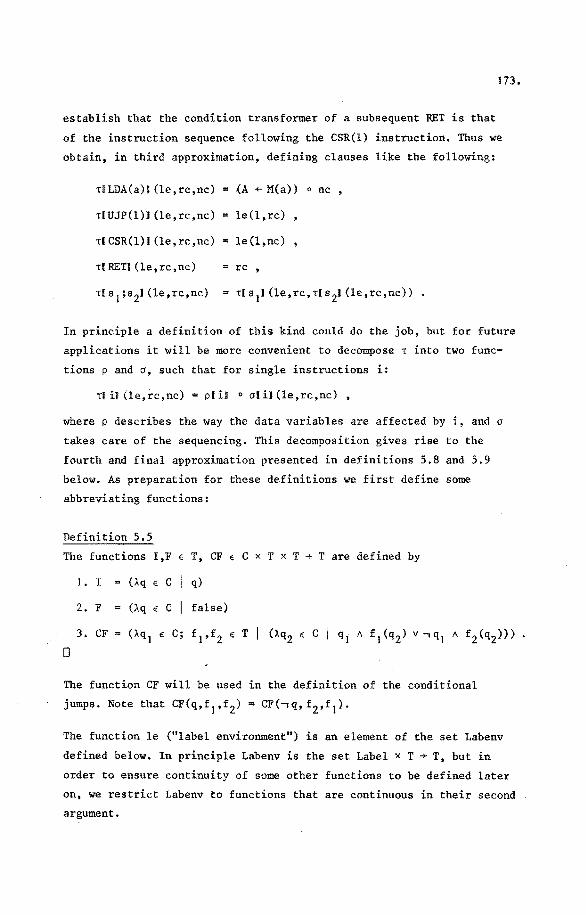
173.
establish that the condition transfarmer of a subsequent RET is that
of the instructien sequence following the CSR(l) instruction. Thus we
obtain, in third approximation, defining clauses like the following:
<ILDA(a)J (le,rc,nc)
<[UJP(l)J (le,rc,nc)
(A + M(a}) o nc ,
le(l,rc)
<[CSR(l)J (le,rc,nc) = le(l,nc)
T(RETJ (le,rc,nc) re ,
In principle a definition of this kind could do the job, but for future
applications it will be more convenient to decompose ' into two func
tions p and cr, such that for single instructions i:
Tl iJ (le,rc,nc) = pliJ 0 olil (le,rc,nc) ,
where p describes the way the data variables are affected by i, and cr
takes care of the sequencing. This decomposition gives rise to the
fourth and final approximation presented in definitions 5.8 and 5.9
below. As preparatien for these definitions we first define some
abbreviating functions:
Definition 5.5
The functions I,F E T, CF E C x T x T ~ T are defined by
0
I. I = (Àq E C
2. F (Àq E C
3. CF
q)
false)
The function CF will be used in the definition of the conditional
jumps. Note that CF(q,f 1,f2) = CF(-,q, f 2,f 1}.
The function le {"label environment") is an element of the set Labenv
defined below. In principle Labenv is the set Label x T ~ T, but in
order to ensure continuity of some other functions to be defined later
on, we restriet Labenv to functions that are continuous in their secoud
argument.

174.
Definition 5.6 {Labenv}
D
I. Labenv = {le E Label x T + T
!for each 1 E Label, each ascending chain <ti>~=O inT:
le(l,iQO ti) = iQO le(l,ti)
2. is the standard order on Labenv.
Lennna 5.7
(Labenv,~LE) is a uccl.
D
Similar to theerem 3.23.2.
D
Definition 5.8 {p, cr}
p E Instructien + T
cr E Instructien + Labenv x T x T + T •
For all le E Labenv, rc,nc E T:
1.1. p[ LDA(a)J = (A + M(a)) •
1.2. crlLDA(a)l (le,rc,nc) = nc
2.1. p(UJP(l)B =I.
2. 2. o( UJP (l)D (le, re, nc) le(l,rc) •
3.1. p[FJP(l)J =I.
3.2. olFJP(l)J (le,rc,nc) CF(Q,nc,le(l,rc)) .
4.1. p(TJP(l)J =I •
4.2. crlTJP(l)J (le,rc,nc) "'CF(ïQ,nc,le(l,rc))
5.1. p(CSR(l)J =I.
5.2. o(CSR(l)B (le,rc,nc) le(l,nc) •

175.
6. I • p( RETJ = I •
6.2. o(RETJ(le,rc,nc) re.
D
Definition 5.9 {T}
T E: Instructien * ->- Labenv x T x T ->- T •
For all leE: Labenv, rc,nc E: T, i E: Instruction, s 1,s2 E: Instruction*:
2. Tl iJ (le,rc,nc) p[il o cri iJ (le,rc,nc) •
D
The following lemma states associativity of T with regard to
Lemma 5.10
For all s 1,s2,s3 E: lnstruction*, le € Labenv, rc,nc ET:
D
D
T[ (s 1 ;s2) ;s3J (le,rc,nc)
{definition 5.9.1}
, T( s 1 ;s2J (le,rc,T[ s3D (le,rc,nc))
{definition 5.9.1}
T[ s 11 (le,rc,TI s2J (le,rc,tl s31 (le,rc,nc)))
{definition 5.9.1}
Tl s 1J (le,rc,Tl s 2;s3J (le,rc,nc))
{definition 5.9.1}
..... ' .

176.
Theorem 5. I I
0
I. For all iE Instructien: cr(iJ E Labenv x T x T +uc T
2. For all s E Instruction*: TlsJ € Labenv x T x T +uc T
Proof
We only prove I for the case i :: UJP(l). The other proofs are similar.
Let <le.>~ 0, <re.>. 0
and <nck>k00
__ 0
be ascending chains in Labenv, T 1 1= J J=
and T, respectively.
n
criUJP(l)J (i~O lei' j~O rcj' ~O nek)
{definition 5.8.2.2}
i~O lei(l,j~O rcj)
{lei E Labenv, definition 5.6}
.ü0 .ü0 le.(l,rc.) 1= J= 1 J
={lemma 3.20.1}
.u0
le. (1, re. ) 1= 1 1
= {definition 5.8.2.2}
.u0 aiUJP(l)J (le.,rc.,nc.) 1= 1 1 1
Finally we define the function ~ which yields the condition transfarmer
of an entire program 10: s0 ; 11
: s 1; ••• ; ln: expressed in those of
its constituent instructien sequences si. Similarly to o in definition
4.26, the label environment le of an entire program is defined as
least fixed point of a function F € Labenv + Labenv. The condition
transfarmer of the program is that of the instructien sequence follow
ing label 10 , i.e. le(l0,rc) for some suitable re. He choose re = F to
ensure that a program aborts if it attempts to execute more RET than
CSR instructions.
Definition 5.12 {w}
~ E Program + T

177.
where
1e = JJF •
and F e: Labenv -+ Labenv is given by
F = (Ue' E Labenv
(U E Label, re E T I [1 = 10 .... Tls0J (le',rc,le'(11,rc))
'
1=1 n-1 -+ T( s 11 (le' ,rc,1e 1 (1 ,re)) • n- n
0
1 1 + I n
In order for this definition to be well-formed, it is necessary that F is continuous. This is ensured by the following theorem.
Theorem 5. 13
0
Proof
F E (Labenv -+ Labenv) • uc
Immediate1y by theerem 5.11 and the "pointwise" lub definition in
Labenv.
0
Example
Consider the programs x, y and z be1ow, which correspond to common
trans1ations of the SL programs
p = B .... s1
; p D -, B ... s2
fi p ,
or do B -+ s1
od; s2 •
Let b, s 1 and s2 be regu1ar instructions.

178.
x .. 1x0: UJP(lx4);
lx1
: b• '
FJP(lx2);
sI; CSR(lx
1);
UJP(lx3);
s2;
lx3: RET;
lx4 : CSR(lx1);
lx5:
y lyo: b;
FJP(ly1);
si; UJP(ly0);
lyl: s2;
ly2:
z = lz0: UJP(lz2);
lz1
: SI;
1z2: b;
TJP(lz1);
sz;
lz3:
By definition 5.12 and the fixed point property we obtain, after
simplification by means of definitions 5.8 and 5.9:

lex (U,rc
[1
1
1
1
1
1
lx0
+ lex(lx4 ,rc)
lx1
+ p(b] o CF(Q,pl s1J o lex(lx
1,1ex(lx
3,rc)),
lex(lx2,rc)) ,
lx2
+ p[ s2J " lex(lx
3,rc) ,
lx4
+ lex(lx 1,1ex(lx5,rc))
lx5 + I
[1 ly0
+ plbl o CF(Q,pls1J o lex(ly
0,rc),lex(ly
1,rc))
1 ly1
+ p[ s2J o ley(ly
2,rc)
1 ly2
+ I
179.
lez = (Àl,rc
[1 1z0
+ lez(lz2,rc) ,
1 = 1z1
+pi s11 o lez(1z
2,rc)
1 1z2
+ p[bJ c CF(ïQ,pls2J o 1ez(1z
3,rc),lez(lz
1,rc)),
1 1z3
+ I
From these equations it follows that

180.
rr( XI
lex(lx0,F)
lex(lx4,F)
lex(lx1
, I)
and
lex(lx1,I)
plbJ o CF(Q,pl s11 o lex(lx
1,I) ,p( ) •
rrl yl
ley(ly0,F)
p(bJ o CF(Q,p[s1J o ley(ly
0,F),pls
21).
1T( zl
lez (lz0 ,F)
lez(lz2,F)
and
lez(lz2,F)
p[b] o CF(-,Q, p( s21 ,p( s11 o lez(lz2,F))
plbl o CF(Q,p[ s 11 o lez(lz2,F),pl s 21) .
We find that rrl xJ , rr[ yl and 1T[ zJ all equal the least solution of the
equation
W: W = plbl o CF(Q,pl s 11 o W,p[ s 2J) ,
hence programs x, y and z are equivalent.
D
The following lemma states a property of the label environment le of
program p which will be used in the derivation of version 2.

181.
Let le be as in definition 5.12.
le = (H € Label, re € T I [1
l=ln-1 + 1J(le,rc,I) ,
D
Proof
1 1 ->- I n
Immediately from the fixed point property and definition 5.9.1.
D

182.
5.3. Version 2: Introduetion of program store
In this section we shall develop a semantics for program p based upon
the representation of p in a program store, i.e. an array of instruc
tions. This representation enables us to refer to arbitrary instruc
tions by means of their index. As a consequence the label environment
of version I can be eliminated. Version 2 makes use of a program store
P, a label-to-address function la, and functions T1 and o'. First we
establish relations between these entities and those of version I.
Subsequently we derive from these relations and the definitions in
version 1 an equation system in termsof P, la, T', o' and n alone.
Let us assume that the instruction sequences s0 , ... ,sn~J of program p
are stored consecutively in an array P(k: O~k<N) of instructions, where
N = (~ j: O~j<n: length(si)).
Let also be given a function la E Label + {0, •· •• ,N} such that:
for all j: 0 ~ j < n: la(l.) is the index in Pof the first J
It follows
Rl.l. for
R1.2. for
Let le be
R2. le
instructien of s .. J
that
all j: 0 ::;:: j < n: P(k: la(lj) ~ k < la(lj+l)) = s . . J
all j: 0 ::;:: j < n: P(k: la (1.) ::;:: k < N) = sj; ••• ;sn-I J
as in definition 5.12. Fr om R1.2 and lemma 5.14 we
(:U E Label, re E T I
[1 10 _,. TIP(k: la(l0) ~ k < NJ (le,rc,I) ,
l=ln_ 1 + dP(k: la(ln-l) ::;:: k < NJ (le,rc,I) ,
1 1 -+ I n
obtain

Definition 5.15 {T', er'}
1. T 1 E {0, ••• ,N} x T + T •
forall j: 0 ~j <N, re ET:
T'(j,rc) = T[P(k: j:Sk<N)J (le,rc,I)
T1 (N,rc) =I.
2. er' E Instructien + {0, .•• ,N} x T + T •
for all iE Instruetion, j: 0 ~ j < N, reET:
er'[i](j,re) = aliJ (le,rc,T' (j+1 ,re)) •
D
An immediate consequence of relation R2 and definition 5.15.1 is
R3. for all 1 E Label, reET: le(l,rc) = T1 (la(l),rc).
Next, we derive arelation between T 1 and a'.
Let j: 0 ~ j < N, reET.
r'(j,rc)
{definition 5.15.1}
TlP(k: j~k<N)I (le,rc,I)
{instruetions stored consecutively}
Tl P(j); P(k: j+1Sk<N)J (le,rc,I)
{definition 5,9}
plP(j)J <> alP(j)J (le,rc 0riP(k: j+lsk<N)J (le,rc,I))
{definition 5.15.1}
p(P(j)J o cr[P(j)J {le,rc,r' (j+1 ,re))
{definition 5.15.2}
p(P(j)J <> a'lP(j)l (j,re)
183.
The result of this derivation, together with the seeond part of defini
tion 5.15.1, are summarized in:

184.
R4. for all j : 0 :> j < N, re E: T:
T' (j ,re) pfP(j)l o cr'lP(j)l (j,re)
T'(N,re) I •
For cr' we derive a relation RS, divided in cases. As the derivations
of all cases have the same structure, we present the
followed by the results. The pattern is:
RS.m. cr'H J(j,re) m
{definition 5.15.2}
E1(cr,le,T',rc,j)
{definition 5.8.m.2}
{R3}
The results are:
RS.I. a'ILDA(a)l (j ,re) T 1 (j+l ,re) .
RS. 2. a'[UJP(l)J (j,rc) = ,• (la(l) ,re)
R5.3. cr'( FJP(l)] (j ,re) CF(Q,T'(j+I,rc),T'(la(l),rc))
R5.4. a'( TJP(l)J (j, re) "'CF{-,Q, T' (j+I.,rc),T 1 (la(l),rc))
R5.5. cr'ICSR(l)1 (j,re) T 1 (la(l),T 1 (j+l,re))
R5.6. cr'l RETJ (j ,re) re •
Finally, from definition 5.12 andrelation R3 we obtain
R6. 1T[pl = t'(la(l0),F)
pattern,
Taken together, relations R4, R5 and R6 are a semantics for p in terros
of P, la, T', cr' and 1T.

185.
5.4. Version 3: Introduetion of return stack
A short inspeetion of relations R4, R5 and R6 of version 2 reveals that
each return continuatien is either F or of the form T'(k,rc), where
k E {O, ••• ,N} and re is an ether return continuation. As a consequence
we can characterize return continuations by means of a stack, repre
sented here by a finite sequence over {O, ••• ,N}. We use a function f
to define the return continuatien represented by such a sequence.
Definition 5.16 {Stack}
Stack = {O, ••• ,N}*
0
Definition 5.17 {f}
f E Stack -+ T
I. f(< >) = F
2. f(<j> Ell s) T'(j,f(s)) •
0
These definitions enable us to replace the equation system of version
2, in terms on P, la, T', cr' and rr, by an equation system in termsof
P, la, T", a" and rr, which is basedon stacks instead of return con
tinuations. We begin with definitions of T" and cr".
Definition 5.18 {T", cr"}
I. T" E {0, ... ,N} x Stack -+ T •
for all j: 0 ~ j ~ N, s E Stack:
T"(j ,s) T'(j,f(s))
2. cr" E Instructien -+ {0, ••• ,N} x Stack -+ T •
for all iE Instruction, j: 0 ~ j < N, reE T:
a"[ iJ (j ,s) = cr'HJ (j ,f(s))
0
From definition 5.18 andrelation R4 we obtain:

186.
R7. for all j: 0 $ j < N, s € Stack:
T"(j ,s) piP (j )D o cr"l P(j )J (j ,s)
T"(N,s) I .
For cr" we derive relation R8 below, divided by cases. The derivations
of the first four cases follow the pattern:
RS.m. a" I i ~ (j, s) m
{definition 5.18.2}
cr'lim1 (j,f(s))
= {R5.m}
E1 (j ,f(s), T' ,la)
{definition 5.18.1}
For R8.5 the derivation is
cr"ICSR(l)D (j,s)
{definition 5.18.2}
cr'l CSR(l)D (j,f(s))
{R5.5}
T 1 (la(l),T' (j+l,f(s))
{definition 5. 17.2}
T'(la(l),f(<j+l> es))
{definition 5.18.1}
T"(la(l),<j+l> es)
For R8.6 the derivation is
cr"l RETJ (j ,s)
{definition 5.18.2}
cr'l RETJ (j,f(s))

{R5. 6}
f(s)
{definition 5.17}
if s = < > + F 0 s
{definition 5.18.1}
<j'> $ s' + T'(j',f(s')) fi
if s = < > + F 0 s = <j'> ® s' + T"(j',s') fi
Thus we obtain
R8. 1. cr"l LDA(a) J (j, s)
R8.2. cr"IUJP(l)J (j ,s)
R8.3. cr"[ F JP (l)J (j, s)
R8.4. cr"[ TJP (1) 1 (j, s)
R8.5. cr"[CSR(l)J (j,s)
T"(j+l ,s) •
T"(la(l) ,s)
CF(Q, T"(j+l ,s) ,T"(la(l) ,s))
CF(oQ,T"(j+l,s),T"(la(l),s))
T"(la(l),<j+l> $ s) •
187.
R8.6. cr"i RETD (j, s) if s = < > + F 0 s = <j'> es'+ T1 (j',f(s')) fi
Finally, for p we derive
Hence
R9.
11[ pJ
{R6}
T'(la(l0), F)
{definition 5.17.1}
T'(la(l0),f(< >))
{definition 5.18.1}
11( pJ T"(la(l0
) ,< >) •
Relations R7, R8 and R9 characterize thesemantics of pintermsof
P, la, T", cr" and 11, using stacks instead of return continuations.

188.
5.5. Version 4: Derivation of an interpreter
In this sectien we will derive an operational description of program p
by means of an interpreter. Apart from the data variables M, A, B and
Q, this interpreter will also use control variables, which are used
for sequencing purposes. The control variables are:
P : array (k: 0 ~ k < N) of Instructien ,
la: Label+ {O, .•. ,N},
ip: {O, .•• ,N}
rs: Stack •
The variables P and la serve the same purpose as in version 2. The
variabie ip is the instructien pointer and indicates the location of
an instructien to be interpreted. The variabie rs is the return stack.
For the interpreter P and la are to be considered as constants. All
sequencing has to be performed by appropriate assignments to ip and rs.
We will code the interpreter in a slight variant of the souree language,
the semantics of which will be obvious. Our aim is to construct the
interpreter in such a way that it has the same condition transformer as
the program p to be interpreted. Relations R7, R8 and R9 will serve as
guideline in the derivation.
To begin with, let us try to construct a repetition
DO = do B + S od
such that
RJO. for all sE Stack, j: 0 ~ j < N:
(ip,rs+j,s) o wp(DO) T"(j,s)
If we succeed in doing so, it fellows from relation R9 and the wp
definition for assignment and sequentia! composition (definitions
3.37.3 and 3.37.4) that the program
ip,rs := la(t0), < >; DO
has the same condition transformer as program p, so we may regard it
as an operaticnat description of p.
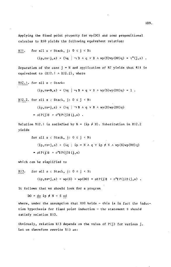
Applying the fixed point property for wp(DO) and some propositional
calculus to RIO yields the following equivalent relation:
Ril. for all s E Stack, j: 0 :::; j :::; N:
189.
(ip,rs+-j,s) o (Àq I ï B 11 q v B 11 wp(S)wp(DO)q) = <"(j,s) .
Separation of the case j = N and application of R7 yields that Ril is
equivalent to (R12.1 11 R12.2), where
Rl2. I. for all s E Stack:
(ip,rs+-N,s) o (Àq I ï B 11 q v B 11 wp(S)wp(DO)q) I •
Rl2.2. for all s E Stack, j: 0:::; j < N:
(ip,rs+-j,s) o (Àq I ïB 11 q v B 11 wp(S)wp(DO)q)
p[P(j)J o o"IP(j)J (j,s)
Relation Rl2.1 is satisfied by B = (ip, N). Substitution in Rl2.2
yields
for all sE Stack, j: 0:::; j < N:
(ip, ,s) o (Àq I ip = N 11 q v ip , N 11 wp(S)wp(DO)q)
p(P(j)J o o"lP(j)J(j,s)
which can be simplified to
Rl3. for all s € Stack, j: 0:::; j < N:
(ip,rs+j ,s) o wp(S} o wp{DO) = p( P(j}J o a"l P(j)J (j ,s) .
It follows that we should look for a program
DO do ip j. N + S
where, under the assumption that RIO holds - this is in fact the induc-.
tion hypothesis for fixed point induction - the statement S should
satisfy relation R13.
Obviously, relation R13 depends on the value of P(j) for various j.
Let us therefore rewrite R13 as:

190.
Rl4. for all s E Stack, j: 0 ~ j < N:
(ip,rs+j,s) o wp(S) o wp(DO)
O.q i [Vi I i E Instrucdon I P{j) i A p( iJ a"( iJ (j ,s)q]) •
This relation is satisfied by
wp(S) = (;l.q I [V i I i E Instrucdon I P (ip)
provided we can find statements Ti such that
for all i E Instruction, s E Stack, j: 0 ~ j < N:
(ip,rs+j,s) o wp(Ti) o wp(DO) pi iJ o cr"( iJ (j ,s)
Let us denote the set Instruction by the k element set {i 1, ••• ,ik} for
a while. As wp(S) is the condition transfarmer of an alternative state
ment with mutually exclusive guards P(ip) = ik' it follows that we
should look for a program
DO = do ip # N ~ if P(ip)
D
od
D P(ip)
fi
i1
+ T. '~]
where, under the assumption that RIO ho.lds, the statements T. should ~
satisfy relation RIS.
Let us restriet ourselves to statements T. of the form ~
where the statements Xi do not contain ;assignments to the variables ip
and rs. In that case relation RIS may be rewritten as:
RJ6. for all i E Instruction, S E Stack, j: 0 s j < N:
wp(Xi) 0 (ip,rs+j,s) 0 wp(Yi) o wp(DO) = pi iJ 0 cr"l iJ (j ,s)
which is implied by (RJ7 A R18), where
Rl7. for all i E Instruction: wp(Xi) = p( iJ •
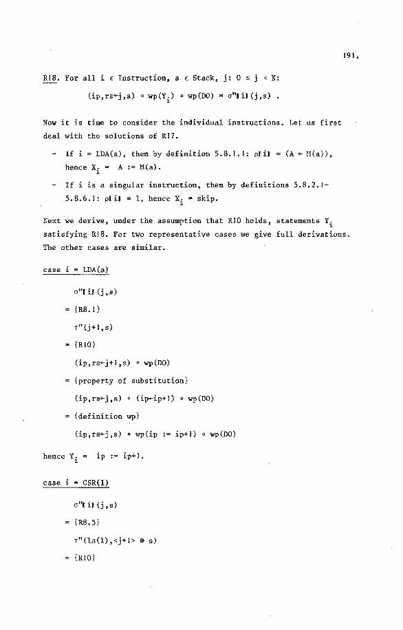
RIS. For all i € Instruction, s € Stack, j: 0 ~ j < N:
(ip,rs+j ,s) o wp(Yi) o wp(DO) = cr"l iJ (j ,s) .
Now it is time to consider the individual instructions. Let us first
deal with the solutions of Rl7.
If i= LDA(a), then by definition 5.S.I.I: plil (A+- H(a)),
hence Xi A:= M(a).
If i is a singular instruction, then by definitions 5.8.2.1-
5.8.6.1: p[iJ =I, hence Xi =skip.
191.
Next we derive, under the assumption that RIO holds, statements Yi
satisfying RIS. For two representative cases we give full derivations.
The other cases are similar.
cr"l iJ (j , s)
{RS. I}
T"(j+l ,s)
{RIO}
(ip,rs+j+l,s) o wp(DO)
{property of substitution}
(ip,rs+j,s) o (ip+ip+l) o wp(DO)
{definition wp}
(ip,rs+j,s) o wp{ip := ip+l) o wp(DO)
hence Y. l.
ip := ip+l.
case i CSR(l)
o"( iJ (j ,s)
{RS.5}
T"(la(l) ,<j+l> !9 s)
{RIO}

192.
(ip,rs+-la(l), <j+l > ~ s) o wp(DO)
{property of substitution}
(ip,rs+-j ,s) o (ip,rs+-la(l), <j+l >EB s) o wp(DO)
{definition wp}
(ip,rs+-j ,s) o wp(ip,rs := la(l), <j+l >EB s) o wp(DO)
hence Y. = ip,rs := la(l),<j+I> EB s . ~
By similar derivations we find
case i UJP(l): Y. = ip := la(l) ~
case i FJP(l): Y. = if Q .... ip := ip+l ~ - 0 ïQ
case i TJP(l): Y. = if ï Q .... ip := ip+l 0 Q ~
case i RET Y. = if s <j' > EB s' -+ ip,rs ~
.... ip := la(l)
.... ip := la(l)
:= j',s' fi
fi
fi
With the .derivation of the statements Xi and Yi we have completed the
derivation of the interpreter. Combination of the code fragments yields:
ip,rs := la(10), < >;
do ip f N -+
if P(ip) LDA(a)
0 P(ip) UJP(l)
0 P(ip) F JP (1)
0 P(ip) TJP(l)
0 P(ip) CSR(l)
0 P(ip) RET
fi
od
-+A := M(a); ip := ip+l
.... skip; ,ip := la(l)
.... skip;
if Q .... ip := ip+l O•Q-+ ip := la(l) fi
-+ skip;
if ï Q .... ip := ip+l 0 Q .... ip := la(l) fi
.... skip; ip,rs := la(l),<j+l> EB rs
.... skip;
if s = <j'> EB s' .... ip,rs := j',s' fi

CHAPTER 6
EPILOGUE
193.
We conclude this thesis with a short summary and evaluation of the results
obtained in preceding chapters.
In chapter 2 we have developed a variant of attribute grammars which is a
self-contained formal system free of implementation bias. Nevertheless, the
various components of this system can be used directly as compiler specifi
cations, from which compilers can be derived by means of existing techniques
for attribute evaluation and data structure implementation. The grammar for
the souree language is rather compact: it has only 33 grammar rules.
We have extended the predicate transfarmer methad to a genuine definition
method by providing it with a firm foundation and extending it to language
constructs other than statements.In this respect the lattice theory of
section 3.1 has been of great value. The general framework provided by this
theory has helped in structuring definitions and in separating general
lattice-theoretical properties from properties particular to certain language
constructs.
We have developed semantics and proof rules for recursive procedures, both
with and without parameters, constructs the formal treatment of which in
the literature has often been problematic. We have succeeded in doing so by
separation of the various aspects of procedures and by making design
choices leading to simple semantics, e.g. with respect to parameter meeha
nisros and initialization requirements.
The background of our work has made it necessary to consider both syntax
and semantics. On the one hand, taking into account context-dependent
properties has complicated various derivations, and we feel that there is
room for impravement in this respec,t. On the other hand, it has enabled us
to derive rather simple conditions for the applicability of certain proof
rules, e.g. with respect to scope of variables and disjointness of para
meters, a notorious problem area.

194.
We have shown that it is possible to give a manageable non-operational
definition of machi.ne instructions, and that an implementation of these
instructions can be derived systematically. The latter derivation also
gives an impression of the way the formalisros developed in this thesis
will be put to work in the derivation of a translation from SL to TL.

APPENDIX A
PROOF OF SOME LEMMAS
Proof of lemma 3.20.2
(C,!;) is a uccl
• {definition 3.5, R, S countable}
(~ i E R, j E s I x ij 5. j'is x ij A j~S x ij !:: i~R j'is x ij)
• {transitivity ~. definition 3.2}
j € s I .UR x .. c: .UR .US x .. ) ~€ ~J - ~E JE ~J
• {definition 3.2}
.US .UR x .. 5. .UR .US x .. JE 1E ~J l.E J€ ~J
Also, by symmetry:
,US .UR x •. ;:. JE ~E ~J - ,US x ••
JE: 1J
Hence, by antisymmetry of ~ :
D
.us JE x ••
1J
Proof of lemma 3.21
• tdefinition n}
(~i I i~ 0 I l'.:i n Yi!: xi+1 A xi n Yi!;. Yi+l)
{definition n}
(~ i I i ~ 0 I x i n y i ;;: x i+ 1 n Y i+ 1 )
<xi n yi>:=O is an ascending chain.
195.

196.
2. Let
We first prove
I. z ~x n y, and subsequently the stronger assertion
2. z x n y.
I. true
{definition n}
• {definition u}
<~ i I i ~ o I {definition n}
{definition u}
x. n ~
iQO (xi n yi) ~ <iQO xi) n <iQO yi)
{definition x, y, z}
z!;xny
2. z s x n y
{definition 3.1}
(z = x n y) v (z c x n y)
{definition x, y, n}
(z = x n y) v (z c
• {definition u}
(z = x n y) v ( i I i~O I z t: xi) A (!i I i?:O I z c yi))
• {<x.>~ 0 and <y.>~ 0 ascending} 1 1= 1 1=
(z = x n y) v (! i i <:: 0 I z c xi A z c yi)
{definition n}
(z = x n y) v
{definition U}
i i~ 0 I z c x. n y.) 1 1

"' (z = xn y) v (ze i':lo (xi n yi))
{definition z}
(z = x n y) v (z c z)
(z = x n y)
0
Proof of lemma 3.22
By induction on the size of S.
0
I. ForS 0 the equality holds, because n 0 = T. c
2. Ind. hyp.: let for some fini te set S'
"' co
i'ds• .wo x .. = .wo i'ds' x .. J"" l.J J'" l.J
Let 1 i S' • and s = {1} u S'.
ro .n
5 .u
0 x ..
l.E J= l.J
{S = {1} u SI} (.uo x .. ) n (.ns, .ü'o x .. ) J= l.J l.E J= l.J
Und. hyp.} ( .ü'o x .. ) n (.uo .ns, x .. ) J= l.J J= l.E l.J
co {lemma 3.21.2} .w0 (x .. n .n5, x .. )
J= l.J l.E 1.]
00
= { s = { 1} u s' } .wo x .. J= l.J
Proof of lemma 3.25
I. g o (~ hi)
{definition lQJ } g o ( Àx I ~ hi (x))
{functional composition} (Àx I g(t§l hi(x)))
{gE D} (Àx I ~ g(hi(x)))
{definition lQJ } lfu (Àx I g(h. (x))) i=O 1
197.

198.
0
= {functional composition} lQJ (g o hi) • i=O
2. (~ gJ 0 (~ hJ {functional composition} (Àx I (~ gi)((~ hj)(x)))
{definition LQJ } ( Àx I ~ gi (~ hj (x)))
~ J.fJ gi (h. (x))) 1=0 ]=0 J •
{lemma 3.20.1} (Àx I~ gk(hk(x)))
= { definition LQJ } l.fu (Àx gk (~(x))) k=O
{functional composition} Lfu (gk 0 hk) . k=O
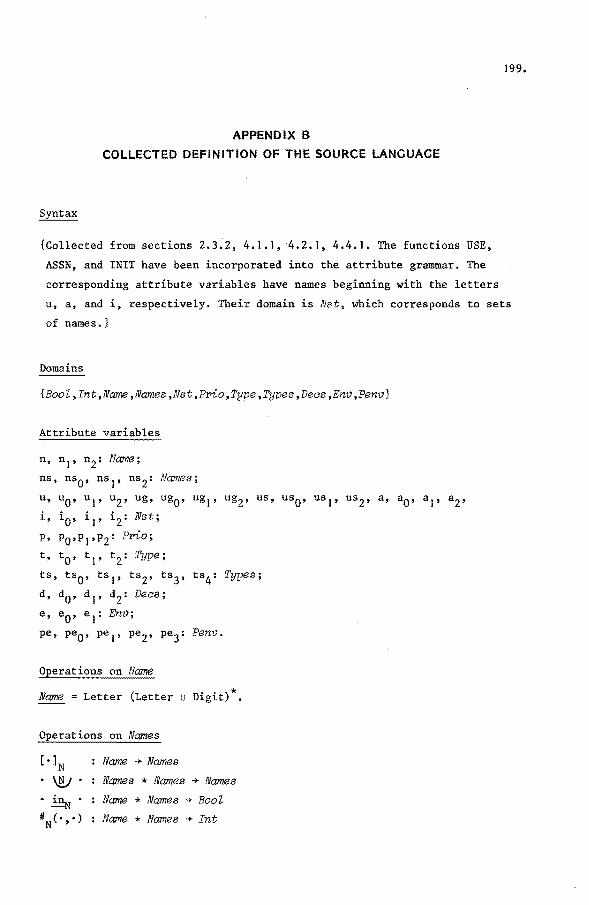
199.
APPENDIX B
COLLECTED DEFINITION OF THE SOURCE LANGUAGE
{Collected from sections 2.3.2, 4.1.1, 4.2.1, 4.4.1. The functions USE,
ASSN, and INIT have been incorporated into the attribute grammar. The
corresponding attribute variables have names beginning with the letters
u, a, and i, respectively. Their domain is Nat, which corresponds to sets
of names.}
Domains
{Bool,Int,Name,Names,Nst,Prio,Type,Types,Deas,Env,Penv}
Attribute variables
n, n 1, n2 : Name;
ns, ns0 , ns 1, ns 2: Names;
u, u0 , u 1, u2 , ug, ug0 , ug 1, ug2 , us, us0 , us 1, us 2 , a, a0 , a 1, a2,
i, i0
, i1
, i2
: Nst;
p, Po•PJ•Pz= FPio; t, t 0 , t
1, t 2 : Type;
ts, ts0 , ts 1, ts2, ts3 , ts4: Types;
d, d0 , d 1, d2 : Deas;
e, e0
, e1
: Env;
pe, pe0 , pe 1, pe2, pe3 : Penv.
Operatiens on Name
Name =Letter (Letter u Digit)*.
[.] N Name + Names
• \!!) • Narnes * Narnes + Names
. ~. Name * Names + Bool
#N( • '•) Name * Narnes +Int

200.
#N (n 1,[n2]N) : if n 1 = n2 +I 0 n 1 ~ n2 + 0 fi
# N
on Nst
Net set of Name. Details of set axioms omitted.
Operatiens on Prio
Prio = {e E Int the integer value corresponding to e is an element
of { I , ••• , 7}} •
Typesym.
Operatiens on Types
Type -• Types
Types * Types +
Narnes * Type +
Mts([n)N,t) = [t]T
Mts(ns 1 ~ns 2 ,t) = Mts(ns 1,t) ~ Mts(ns 2,t)
on Deas
[•,•]D Narnes * Type + Deas • \!?). De as * Dees + Dees
(. '.) i~ • Name * Type * Deas + Bool # D ( •' •) Name * Deas + Int

#N (n,ns) #D (n, [ns, t]D)
#n (n,dl \W dz) #D (n,dl) + #D (n,d2)
Operations on Env
Empty Env
Ext(•,•) Env * Deas + Env
(•,·) i~ • Name* Type* Env + BooZ
(n,t) ~ Empty = false
(n,t) ~ Ext(e,d) = (n,t) d V (#D (n,d)
Operations on Penv
Pempty Penv [. • • 1
' ' p Name * Types * Types + Penv
. \V . Penv * Penv + Penv # p(•,•) Name * Penv + Int
0 11 (n, t)
(•,•,•) inp . Name * Types· * Types * Penv + BooZ
# (n,Pempty) = 0 p
#p
# p
(n1, [n2,ts 1, ts21P) = if n1 = n2 + I D n1 f< n2 + 0 fi
(n,pe1
\g/pe2 ) = #P (n,pe 1) + #P (n,pe2 )
(n,ts 1,ts2) ~ Pempty = false
(n1,ts 1,ts2) ~ [n2,ts3 ,ts4lp
VN {Abstr <Penv,Types,Types> ,
Block <Penv,Env,Nst,Nst,Nst> ,
Con <Type> ,
Decs <Deas> ,
Dop <FPio,Type,Type,Type> ,
Expr <Env,Prio,Type,Nst> ,
Exprs <Env,Types,Nst> ,
201.
e)

202.
Gcs <Penv,Env,Nst,Nst,Nst,Nst> ,
Id <Name> ,
Ids <Names>
Mop <Type,Tyve> ,
Pdecs <Decs,Types> ,
Procdecs <Penv,Penv> ,
Prog ,
Stat <Penv,Env,Nst,Nst,Nst> ,
Type <Type> ,
Var <Env,Name,Type> ,
Vars <Env,Names,Types,Nst>
Terminals
Letter {"a", ... ,"z"}
Digit {"0", ... ,"9"}
Opl {"+", "-", "-."}
Op2 {"*","+","-","=","=f","<","$u,n).n,n~n,nAn,nyn,n::o.","~"}
Typesym {"int","bool"}
Consym {"true","false"}
Statsym {"skip","abort"}
Sym ={"I[","] l","l",",",":",";", "IJ","-+",":=","(",")",
"if","fi","do","od","var","con","res"}
VT Letter u Digit u Opl u Op2 u Typesym u Consym u Statsym u Sym .
Start symbol
Prog.
Pseudo terminals
{Id <Name>, Dop <Prio,Type,Type,Tyve>, Mop <Type,Type>, Con <Tyne>,
Type <Type>}
For all n E Name:
L(Id <n>) = {n} \ (Typesym u Consym u Statsym) .
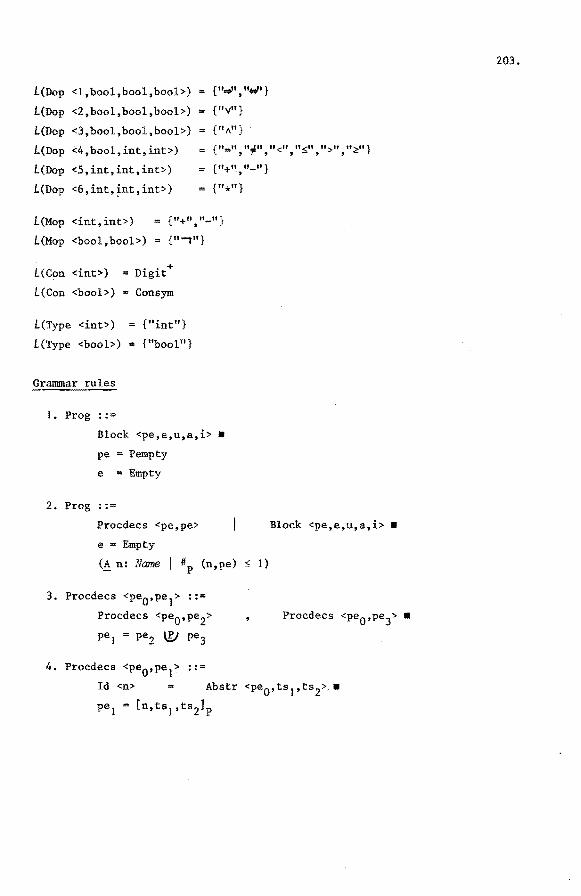
L(Dop <l,bool,bool,bool>) ., { ....... ' "*'' } L(Dop <2,bool,bool,bool>) { "v"}
L(Dop <3,bool,bool,bool>) a { 11 A11 }
L(Dop <4,bool,int,int>) {"=",":f."t"<","sn,n>n,n~u}
L(Dop <5,int,int,int>) {"+","-"}
L(Dop <6,int,~nt,int>) {"*"}
L(Mop <int, int>) {"+", "-"}
L(Mop <bool,bool>) = {"ï"}
L(Con <int>) Digit+
L(Con <bool>) = Consym
L(Type <int>)
L(Type <bool>)
Grammar rules
1. Prog : :=
{"int"}
{"bool''}
Block <pe,e,u,a,i> •
pe = Pempty
e = Empty
2. Prog : :=
Procdecs <pe,pe>
e • Empty
(~ n: Name I #p (n,pe) s 1}
3. Procdecs <pe0,pe1> ::=
Procdecs <pe0,pe2>
pel = pe2 \V pe3
4. Procdecs <pe0,pe 1> ::=
Block <pe,e,u,a,i> •
Id <n> Abstr <pe0,ts 1,ts2>,•
pe 1 = [n,ts1,ts2lp
203.
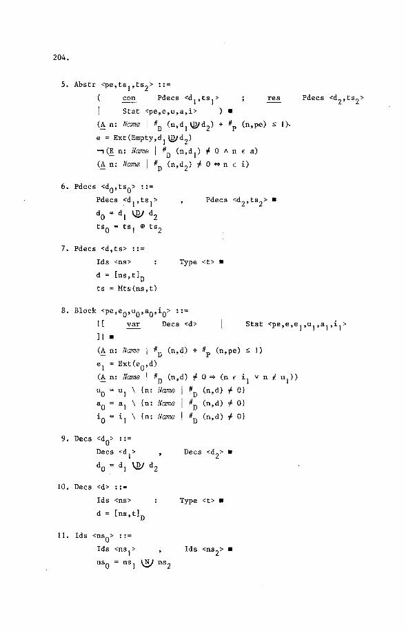
204.
5. Abstr <pe,ts1,ts2> ::=
( con Pdecs <d1,ts
1>
I Stat <pe,e,u,a,i> } •
(!!_ n: Name I # D (n,dl \Wdz) + # p
e Ext(Empty,d1
'JVd2
)
-,(~ n: Name I #0
(n,d1) + 0 A n
n: Name I #0
(n,d2) ; 0 * n E
6. Pdecs <d0 ,ts0> ::=
Pdecs ~d 1 ,ts 1 > do .. dt \BI dz
ts0
= ts1
e ts2
7. Pdecs <d,ts> ::=
lds <ns>
d = [ns,t] 0 ts = Mts(ns,t)
Type <t> •
8. Block <pe,e0 ,u0 ,a0,i0> ::=
I[ var Decs <d>
ll •
(n,pe)
E a)
i)
(A n: Name I #0
(n,d) + #P (n,pe) $ I)
e1
= Ext(e0
,d)
res
$ I~
(!!_ n: Name I #D (n,d) ; 0=> (n E i1
v n i u1))
uo = UI \ {n:
ao al \
ia = i) \
9. Decs <d0
> ::=
Decs <d1>
{n:
{n:
do = dl \!V dz
JO. Decs <d> ::=
Ids <ns>
d = [ns, t] 0
11. Ids <ns0> ::=
Ids <ns 1>
Name
Name
Name
ns0 = ns 1 ~ ns 2
I # (n,d) # 0} D
I # (n,d) # 0} D I #D (n,d) # 0}
Type <t> •

12. Ids <ns> ::•
Id <n> •
ns = [n]N
13. Stat <pe,e,u,a,i> ::=
abort •
u = 0 a = 0 i = 0
14. Stat <pe,e,u,a,i> ::~
skip •
u = 0 a = 0 i 0
15. Stat <pe,e,u0 ,a0,i0> ::=
Vars <e,ns,ts,a0> := Exprs <e,ts,u0> •
<A n: Name I #N (n,ns) ~ I)
io = ao \ uo
16. Stat <pe,e,u0 ,a0,i0> ::=
Stat <pe,e,u1,a
1,i
1> Stat <pe,e,u2 ,a2,i2> •
uo UI u uz
ao = al u a2 io i! u (i2 \ u))
17. Stat <pe,e,u,a,i0> ::=
if Gcs <pe,e,ug,us,a,i 1> fi •
U = ug U US
io .. il \ ug
18. Stat <pe,e,u,a,i0
> ::=
u
Gcs <pe,e,ug,us,a,i 1>
ug U US
19. Stat <pe,e,u,a,i> ::=
Block <pe,e,u,a,i> •
•
205.
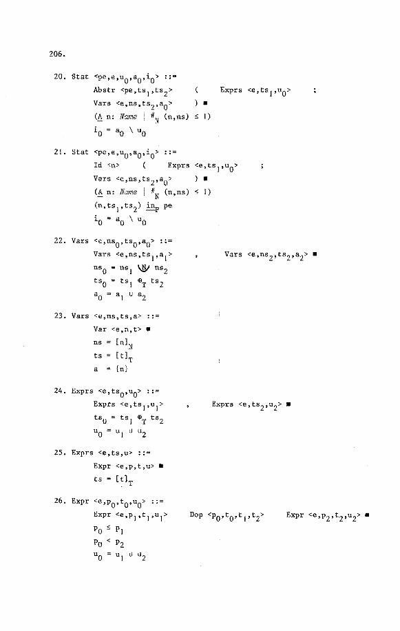
206.
20. Stat <pe,e,u0
,a0,i
0> ::=
Abstr <pe,ts 1,ts2>
Vars <e,ns,ts 2,a0 > ) •
(~ n: Name I #N (n,ns) ~ I)
io = ao \ uo
21. Stat <pe,e,u0
,a0,i
0> ••
Id <n> ( Exprs <e,ts1,u
0>
) . Vars <e,ns,ts2,a0
>
(~ n: Name I #N (n,ns) ~ I)
(n,ts 1,ts2) pe
io = ao \ uo
22. Vars <e,ns0,ts
0,a
0> ::=
Vars <e,ns,ts1,a
1>
ns0
ns1 ~ ns2
ts0 ts 1 eT ts 2 a
0 = a
1 u a
2
23. Vars <e,ns,ts,a> ::=
Var <e,n,t> •
ns [n]N
ts [t]T
a {n}
24. Exprs <e,ts0
,u0> ::=
Exprs <e,ts1,u
1>
ts0 "' ts 1 E9T ts2 u 0 "' u 1 u u 2
25. Exprs <e,ts,u> ::=
Expr <e,p,t,u> •
ts "' [t)T
26. Expr <e,p0,t0 ,u
0> ::=
Expr <e,p 1,t 1,u1>
Po ~ PI
Po < Pz u
0 u
1 u u
2

27. Expr <e,p0,t0 ,u> ::=
Mop <t0,t
1> Expr <e,p
1,t 1,u> •
Po 7 7
28. Expr <e,p0 ,t,u> ::=
Expr <e,p1,t,u> ) •
7
29. Expr <e,p,t,u> ::=
Var <e,n,t> •
p 7
u {n}
30. Expr <e,p,t,u> ::=
Con <t> •
p 7
u 0
31. Var <e,n,t> ::=
Id <n> •
(n,t) ~ e
32. Gcs <pe,e,ug0,us0 ,a0 ,i0> : : ==
Gcs <pe,e,ug1,us 1,a1,s 1>
u go ugl u ug2
uso US) u us2 ao al u a2
io i I n i 2
33. Gcs <pe,e,ug,us,a,i> ::=
Expr <e,p,t,ug>
t = bool
Stat <pe,e,us,a,i> •
207.

208.
Semantics
{Collected from definitions 4.46, 4.47, 4.48, 4.49.}
Definition {wp'}
For all e E Env the function
wp' E L(Stat <Penv,e,Nst,Nst,Nst>) + /':, + T e e
is defined by
0
I. wp' (abort) o O.q E c false) e e
2. wp' (skip) o (Àq E c q) e e
3. wp' (v := E)o (v + E) e
4. wp~(S 1 ;s2 )ö (wp~(s 1 )o)o(wp~(s2)o)
5. wp~(if B1 + s 1 D ... D B ~ s fi)o = n n-
= (Àq E Ce I [V i I l~i::;n I B.] 11 [/\i l
J~i~n Bi~ (wp~(Si)ê)q])
6. wp~ (do B1 ~ s
1 D ••• D Bn ~ Sn od)ö = ]JF ,
where F = (Àf E C + C I e uc e
(Àq E. Ce ([Vi
11 [/\i
7. wp~(A(E;v))o = pwp~(A)(ê)(E,v)
8. wp~(p(E;v))ö = pwp~(p)(o)(E,v)
l$i$n B.] V q) l -
l::;i~n B. ~ (wp'(S.)o) f q])) 1 e 1
9. wp'( I[ var x: tI S ]I ) (Àq E Ce I (wp' ((x+ y)S)o)q) , e - e1
where y E Name such that ~ new (y,e) ,

Definition {wlp'}
For all e E Env the function
wlp' E L(Stat <Penv,e,Nst,Nst,Nst>) + à + T e e
is defined by
D
I. wlp' (abort) o e
2. wlp~ (skip) a
3. wlp' (v := E)o e
(),q E Ce true)
(:\q E Ce q)
(v +- E)
4. wlp~(s 1 ;s2 )ä = (wlp~(S 1 )ä)o(wlp~(S2 )o)
5. wlp~ (if B1 + s 1 D ••• D Bn + Sn
= (Àq E C I [Ai I Js:;L>n I B. • (wlp'(S.)o}q]}i e ~ e ~
6. wlp~(do B1 + s 1 D ... D Bn +Sn od)o = vG ,
where G = (Àf E Ce +de Ce I (;\q é C ([\/i Js:;is:;n B.] V q)
e ~
" [Ai lsis:;n B. • (wlp'(S.)o} f q])) 1. e ~
7. wlp~(A(E;v))o = pwlp~(A)(o)(E,v)
8. wlp~(p(E;v))o = pwlp~(p)(o)(E,v)
9. wlp'( I[ var x: t I S ]I ) = (Àq E C (wlp' ((x+- y)S)o)q) , e e e 1
where y E Name such that ~ new (y,e) ,
e 1 = Ext(e,[y,t]D) •
Definition {pwp',pwlp'}
For all e E Env the functions pwp~ and pwlp~
E L(Id <Name>) u L(Abstr <Penv,Tyves,Tynes>) + à+ P e
are defined as follows:
209.

210.
Let (~x: t1
; res y: t2
I S) E L(Abstr <Penv,Types,Tyves>),,
E = L(Expr <e,Prio,t 1,Nst>) ,
0
V = L(Var <e,Name,t2
>) ,
x' ,y' E Name such that ~ new (x' ,e), ~ new (y',e), x' 1 y' ,
S' = (x,y +x' ,y')S •
l.I. pwp~((con x: t 1; res y: t2
I S))o
= (:\E E E, v E V I (x'+ E) o wp',(S')o o (v + y')) • e
1.2. pwp' (p)ó = ö(p)(e) e
2.1. pwlp~((con x: t 1; ~ y: t 2 I S))ö =
= (ÀE E E, v E V I (x'+ E) <> wlp',(S')o o (v + y')) . e
2.2. pwlp~(p)ö = ö(p)(e) .
Definition hvp and wlp for programs}
l.I. wp(B) = wp~(B)6,
where e = Empty, 6 = 0
where e = Empty ,
and, for i: ~ i ::; k:
~i·= (À~i·····~k Ex I
(Àe E Env I pwp~(Ai){(p 1 .~j), ... ,(pk'~k)}))
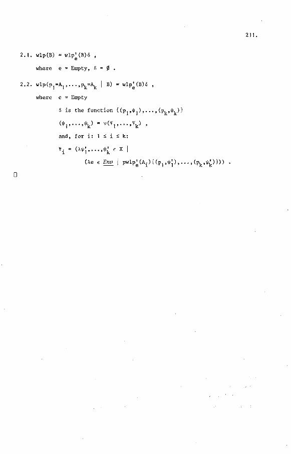
0
2.1. wlp(B) = wlp'(B)o , e
where e = Empty, o ~ •
where e = Empty
B) = wlp' (B)o , e
ê is the function {(p 1,$ 1), ••• ,(pk,$k)}
($1, ••• ,$k) v('jll''''''jlk)
and, for i: ~ i ~ k:
'jli <Àwj •... ,wk Ex 1
(Àe E Env I pwlp~(Ai){(p 1 ,wj), .•. ,(pk,$k)})) •
21 I,

212.
INDEX OF DEFINITIONS
{Unless indicated otherwise, numbers refer to numbers of definitions.}
admissible 3.30
ambiguity 2.8
ascending chain 3.2
attribute grammar 2.12
attribute structure 2.9
attributed derivation tree 2.9
attributed nonterminal 2.14
attributed nonterminal form 2.14
base grammar 2.25
base rule 2.24
base symbol 2.23
base tree 2.26
boolean attribute
cel 3.6
chain 3.3
cl 3.7
structure
complete lattice 3.7
2.10
complete partially ordered set 3.4
conjunctively 3.17
context-free grammar 2.1
continuity 3.19
countably complete lattice 3.6
cpo 3.4
deel 3.5
derivation tree 2.4
deseending chain 3.2
disjunctivity 3.17
domain 2.9
downward continuous 3.19
downward countably-complete
lattice 3.5
expression signature 2.9
fixed point 3.27
frontier 2.5, 2.20
full attributed derivation tree 2.21
full derivation tree 2.6
function signature 2.9
function symbol 2.9
glb. 3.2
grammar rule 2.12
greatest fixed point 3.27
greatest lower bound 3.2
language generated by
grammar 2.3, 2.18
least fixed point 3.27
least upper bound 3.2
lub 3.2
monotonicity 3.14
non-logical axioms 2.9
nonterminal 2.1, 2.12
nonterminal signature 2.12
partial correctness logic 3.51
partial correctness proef rule 3,49
partially ordered set 3.1
production rule 2.1
proof rule 3.49
pseudo terminal sections
rule condition 2.12
rule form 2.12
standard order 3.9
start symbol 2.1
strictness 3.12
substitution 2.15
2. J .2,
2.2.2

substitution in conditions
note following 3.38
substitution in statements 4.6,
4. 14
terminal 2.1, 2.12
total correctness logic 3.53
total correctness proof rule 3.49
{notions pertaining to grammars}
>> 2.2, 2.57
+ >> 2.2, 2.17
* >.> 2.2, 2.17
L 2.3, 2.18
D 2. 11
es 2. 13
AN 2. 14
pr 2. 16
bs 2.23
br 2.24
bt 2.26
{notions pertaining to lattices}
(C,E,) 3. I
~ 3. I
c note following 3.1
.2 note following 3.1
n 3.2, 3. 16
u 3.2, 3. 16 <X)
r:1o x. 3.2 l.
<X)
u x. 3.2 i=O .].
.L note on P· 57
T note on P• 57
uccl 3.5
upward continuous 3.19
upward countably-complete
lattice 3.5
variabie signature 2.9
vocabulary 2.1
{notions pertaining to condition
transformers}
eq 3.31
Ce 3.32
1:' 3.33 -e T 3.35 e p 4. 15 e /:; 4. 21' 4.45
x 4.42
213.
wp 3.37, 4. 10, 4.18, 4.26, 4.49
wp' 4.23, 4.46
wlp 3.38, 4.1 0, 4. 18, 4.26, 4.49
wlp' 4.24, 4.47
pwp 4.17
pwp' 4.48
pwlp 4. 17
pwlp' 4.48
(v + E) note following 3.38
(x + y) 4.6, 4.14
USE 4.1, 4. 13
ASSN 4.2, 4. 13
INIT 4.3, 4.13

214.
{notions pertaining to proof rules} {notions pertaining to target
PvalidO 3.48 language}
Pvalidl 4.29 Stack 5.16
Pvalid2 4.34 Instruction 5.1
Pvalid3 4.51 Label 5.2
Pvalid4 4.57 Labenv 5.6
PsoundO 3.50 T 5.3
Psound1 4.30 I,F,CF 5.5
Psound2 4.35 f 5.17
Psound3 4.52 p 5.8
Psound4 4.58 rJ 5.8
Tv a lidO 3.48 cr' 5. IS
Tvalidl 4. 37 cr" 5.18
Tvalid2 4.62 T 5.9
TsoundO 3.50 TI 5.15
Tsound1 4.38 , .. 5.18
Tsound2 4.63 1T 5. 12
PC0 3.51
PA1,PA2 3.51
PR1, ••• 3.51
PRs,PR6,PR7 4.11
PRa,PRg 4.19
PR 10 ,PR1 I 4.55
PR12 following th. 4.61
TCO 3.53
TA1 , TA2, TA3 3.53
TRI, ••. ,TR4 3.53
TR5, •.. , TR7 4.11
TR8,TRg 4.19
TRIO'TRII 4.66
TRI2 following th. 4. 68

[Apt I)
[Apt 2]
[Ashcroft]
[Back I]
[Back 2]
REFERENCES
Apt, K.R., Ten years of Hoare's logic: A survey- Part I.
ACM Transactions on Programming Languages and Systems ~. 4
(Oct. 1981), pp. 431-483.
215.
Apt, K.R., A sound and complete Hoare-like system fora fragment
of Pascal, Report IW 97/78 Mathematisch Centrum, Amsterdam, 1978.
Ashcroft, E.A., Wadge, W.W., Rj for 'Semantics, ACM Transactions
on Programming Languages and Systems ~. 2 (Apr. 1982), pp. 283-294.
Back, R.J.R., Proving total correctnessof nondeterministic
programs in infinitary logic, Acta Inf. ~ (1981), pp. 233-249.
Back, R.J.R., Correctness preserving program refinements: proof
theory and applications, Mathematica! Centre Tracts 131, Mathema
tisch Centrum, Amsterdam, 1980.
[de Bakker]
[Bjl!irner]
[Bochmann]
de Bakker, J.W., Mathematical theory of program correctness,
Prentice-Hall, 1980.
Bjl!irner, D., Jones, C.B. (eds.), The Vienna development method:
the meta language, Lect. Not. Comp. Sci. ~. Springer, 1978.
Bochmann, G.V., Ledgard, H.F., Marcotty, M., A sampler of formal
definitions, ACM Computing Surveys~. 2 (June 1976), pp. 191-276.
[Brinch Hansen]
Brinch Hansen, P., Concurrent Pascal Report, Information Science,
California Institute of Technology, 1975.

216.
[Cook I]
[Cook 2]
[Curry]
Cook, S.A., The complexity of theorem-proving procedures. Procs.
3rd Ann. ACM Symp. on theory of computing, May 1971.
Cook, S.A., Soundness and completenessof an axiom system for
program verification, SIAM J, on Computing I• 1978, pp. 70-90.
Curry, H.B., Feys, R.
Combinatory logic, vol. I., North-Holland Publ. Comp., 1958.
[Dijkstra I]
Dijkstra, E.W., Guarded commands, nondeterminacy and formal
derivation of programs, Comm. ACM ~. 8 (Aug. 1975), pp. 453-457.
[Dijkstra 2]
Dijkstra, E.W., A discipline of programming, Prentice-Hall, 1976.
[Dijkstra 3]
[Floyd]
[Ginsburg]
[Goguen]
[Gut tag]
Dijkstra, E.W., Lecture notes "Predicate transformers" (Draft),
EWD 835, 1982.
Floyd, R.W., Assigning meanings to programs, Proc. Symp. in
Applied Mathernaties 19, Mathematica! Aspects of Computer Science,
J.T. Schwartz (ed.). AMS 1967, pp. 19-32.
Ginsburg, S., Rounds, E.M., Dynamic syntax specificatien using
grammar forms, IEEE Trans. Soft. Eng., vol. SE-4, no. 1, Jan. 1978,
pp. 44-55.
Goguen, J.A., Thatcher, J.W., Wagner, E.G., An initial algebra
approach to the specification, correctness, and implementation of
abstract data types; in: Current Trends in Programming Methodology,
~. R.T. Yeh (ed.), Prentice-Hall, 1978, pp. 80-149.
Guttag, J.V., The specificatien and application to programming of
abstract data types, Ph.D. thesis, Comptr. Syst. Res, Group Tech.
Rep. CSRG 47, Dept. Comptr. Sci., Univ. of Toronto, 1975.

[Hemerik]
[Hoare 1]
[Hoare 2]
[Hoare 3]
[Jazayeri]
[Knuth]
[Karp]
[Lauer]
[Ledgard]
217.
Hemerik, C., Relaties tussen taaldefinitie en taalimplementatie
(in Dutch), MC Syllabus 42, J.C. van Vliet (ed.), Mathematisch
Centrum, Amsterdam, 1980, pp. 109-142.
Hoare, C.A.R. An axiomatic basis for computer programming, Comm.
ACM I!• 10 (Oct. 1969), pp. 576-580.
Hoare, C.A.R., Wirth, N., An axiomatic definition of the program
ming language Pascal, Acta Inf. !• 1973, pp. 335-355.
Hoare, C.A.R., Procedures and parameters: an axiomatic approach;
in: Symp. on Semantics of Algorithmic Languages, E. Engeler (ed.),
Lect. Not. Math. 188, Springer, 1971, pp. 102-116.
Jazayeri, M., Ogden, W.F., Rounds, w.c., The intrinsically ex
ponentional complexity of the circularity problem for attribute
grammars, Comm. ACM ~. 12 (Dec. 1975), pp. 697-706.
Knuth, D.E., Semantics of context-free languages, Math. Syst.
Theory! (1968), pp. 127-145. Correction in: Math. Syst. Theory 5
(1971), p. 95.
Karp, C.R., Languages with expressionsof infinite length, North
Holland Publ. Comp., 1964.
Lauer, P.E., Consistent formal theoriesof thesemantics of
programming languages, Tech. Rep. TR. 25.121, IBM Lab. Vienna,
Nov. 1971.
Ledgard, H.F., Production systems: a notation for defining syntax
and translation, IEEE Trans. Soft. Eng., vol. SE-3, no. 2, March
1977, pp. 105-124.

218.
[Me Carthy]
[Milne]
[Plotkin]
[Räihä]
[Scott I]
[Scott 2]
[Simonet]
[Strachey]
[Stoy]
Me Carthy, J., Towards a mathematica! science of computation,
Procs. IFIP Congress 62, C.M. Popplewell (ed.), North-Holland
1963, pp. 21-28.
Milne, R.E., Tranforming predicate transformers, Proc. IFIP TC-2
Working Conference on Formal Description of Programming Concepts,
E.J. Neuhold (ed.), North-Holland, 1978, pp. 31-65.
Plotkin, G.D., Dijkstra's predicate transformers and Smyth's
power domains, Procs. 1979 Copenhagen Winter School, D. Bj~rner
(ed.), Lect. Not. Comp. Sci. 86, Springer~ 1980.
~ihä, K.-J., Bibliography on attribute grammars, ACM SIGPLAN
Notices ~. 3 (March 1980), pp. 35-44.
Scott, D.S., Logic with denumerably long formulas and finite
strings of quantifiers, Symp. on the Theory of Models, J. Addison,
L. Henkin, A. Tarski (eds.), North-Holland, 1965, pp. 329-341.
Scott, D.S., Data types as lattices, SIAM J. on Computing ~.
1976, pp. 522-587.
Simonet, M., An attribute description of a subset of ALGOL 68,
Proc. of the Strathclyde ALG0L 68 Conf., ACM SIGPLAN Notices I 6
(June 1977), pp. 129-137.
Strachey, C., Wadsworth, C.P., Continuations: a mathematica!
semantics for handling full jumps, Technica! Monograph PRG-11,
Programming Research Group, University of Oxford, 1974.
Stoy, J., Denotational semantics: the Scott-Strachey approach to
programming language theory, MIT Press, 1977.

[Tennent]
[Wand]
[Watt]
[Wegner]
[Wirth I]
[Wirth 2]
219.
Tennent, R.D., Language design methods basedon semantic principles.
Acta Inf.~ (1977), pp. 97-112.
Wand, M., A characterization of weakest preconditions, J. Comp.
Syst. Sci. ~. 1977, pp. 209-212.
Watt, D.A., An extended attribute grannnar for Pascal, SIGPLAN
Notices ~. 2 (Feb. 1979), pp. 60-74.
Wegner, P., The Vienna Definition Language, Computing Surveys~.
1972, pp. 5-63.
Wirth, N., Weber, H., EULER: A Generalization of ALGOL, and its
Formal Definition, part II, Comm. ACM ~. 2 (Feb. 1966), pp. 89-99.
Wirth, N., Hoare, C.A.R., A contribution to the development of
ALGOL, Comm. ACM ~. 6 (June 1966), pp. 413-431.
[van Wijngaarden]
van Wijngaarden, A. et. al. (eds.), Revised report on the algo
rithmic language ALGOL 68, Acta Inf. ~. 1975, pp. 1-236.

220.
SAMENVATTING
Het onderzoek waarvan in dit proefschrift verslag wordt gedaan maakt deel
uit van een meer omvattend project dat tot doel heeft het op systematische
wijze construeren van correcte implementaties van programmeertalen. De
volgende aspecten spelen daarbij een rol:
1. De definitie van de brontaal.
2. De definitie van de doeltaal.
3. De constructie van een "betekenis behoudende" afbeelding van brontaal
naar doeltaal.
4. De constructie van een programma dat die afbeelding realiseert.
Het is duidelijk welke afhankelijkheden er tussen deze aspecten bestaan:
3 is uitsluitend afhankelijk van 1 en 2, en de specificaties van 4 zijn
gebaseerd op I en 3. Het is ook duidelijk dat de correctheidsoverwegingen
van 3 en 4 gescheiden kunnen worden en dat de betrouwbaarheid van de
resulterende vertaler uiteindelijk bepaald wordt door de mate van precisie,
volledigheid en ondubbelzinnigheid van I en 2.
Het onderwerp van dit proefschrift is het ontwerp en de formele definitie
van een brontaal SL en een doeltaal TL, die dienen als uitgangspunt voor
een implementatieproces zoals boven geschetst. Bovendien worden de daarvoor
benodigde definitiemethoden zover als nodig ontwikkeld. Gezien de gegeven
achtergrond zal het echter duidelijk zijn dat dit proefschrift niet be
schouwd dient te worden als een op zichzelf staande studie van taaldefini
tie. Het grootste deel van het beschreven werk is bedoeld als theoretische
fundering van het genoemde implementatieproces.
In het proefschrift wordt allereerst kort ingegaan op voorwaarden waaraan
formele taaldefinities dienen te voldoen, zoals beschikbaarheid van goede
wiskundige theorie en afwezigheid van overspecificatie en implementatie
aspecten. Vervolgens wordt in hoofdstuk 2 de syntactische definitie van de
brontaal behandeld. Het belangrijkste onderwerp van dit hoofdstuk is de
ontwikkeling van een variant van de welbekende attribuutgrammatica's
{Knuth], die primair gericht is op taalspecificatie. De belangrijkste

221.
componenten van deze variant zijn een verzameling geparameteriseerde produk
tieregels en een zogenaamde attribuutstructuur, met behulp waarvan eigen
schappen van parameters uit gegeven axioma's afgeleid kunnen worden.
Enerzijds kan een attribuutgrammatica van deze soort beschouwd worden als
een zuiver formeel systeem gebaseerd op herschrijfregels en logische
afleidingen. Anderzijds kan de attribuutstructuur, die overeenkomt met een
algebraïsche type-specificatie in de zin van [Goguen, Guttag), direct ge
bruikt worden als specificatie van dat deel van een vertaalprogramma, dat
de context-afhankelijke analyse uitvoert.
In hoofdstuk 3 wordt de basis gelegd voor de semantische definitie van bron
en doeltaal. De gebruikte definitiemethode is in essentie die van de
"predicate transformers" [Dijkstra 1, Dijkstra 2]. Deze methode wordt eerst
gefundeerd met behulp van een variant van Scott's "theory of continuous
lattices" [Scott 2] en "infinitary logic" [Back 1, Karp]. Daarna worden de
predicate transfarmers voor een deel van de brontaal in dit raamwerk be
schouwd. Tenslotte worden deze resultaten gebruikt om logische systemen in
de stijl van [Hoare 1, Hoare 2] te ontwikkelen voor het bewijzen van par
tiële en totale correctheid.
In hoofdstuk 4 worden de methoden van hoofdstukken 2 en 3 toegepast op
andere constructies van de brontaal, te weten blokken en procedures. Voor
deze construc-ties worden syntaxis, semantiek en bewijsregels ontwikkeld. De
verschillende aspecten van procedures worden zoveel mogelijk in isolement
behandeld. De behandeling van blokken in sectie 4.1 dient voornamelijk om
de effecten van het introduceren van lokale namen te onderzoeken. In sectie
4.2 worden aan de hand van zogenaamde abstracties de gevolgen van paramete
risering bestudeerd. In sectie 4.3 wordt met behulp van de lattice theory
van sectie 3.1 een betrekkelijk eenvoudige behandeling van parameterloze
recursie gegeven. Tenslotte worden in sectie 4.4 de verscheidene aspecten
samengevoegd, hetgeen resulteert in een behandelin~ van recursieve proce
dures met parameters.
In hoofdstuk 5 worden enige aspecten van de formele definitie van de doel
taal behandeld, met name die welke betrekking hebben op instructies die de
volgorde van verwerking beÏnvloeden, zoals sprongen en subroutine-aanroepen.
Het doel van dit werk is het ontwikkelen van predicate transfarmers voor
machine-instructies, die vervolgens gebruikt kunnen worden bij het constru-

222.
eren van correcte implementaties. In eerste instantie wordt met behulp van
de lattice theory uit sectie 2.1 en de techniek van de "continuations"
[Strachey] een predicate transfarmer semantiek ontwikkeld. Vervolgens
wordt uit deze definitie via enige transformaties een equivalente operatio
nele beschrijving door middel ·van een interpretator-programma afgeleid.
Deze afleiding is zowel een bewijs van de consistentie van twee definities
als een voorbeeld van het afleiden van een implementatie uit een niet
operationele definitie. Bovendien geeft deze afleiding ook een indruk van
de semantiek behoudende transformaties die bij de vertaling van brontaal
naar doeltaal een rol zullen spelen.
Hoofdstuk 6 bevat een korte nabeschouwing van het werk.
Appendix A bevat bewijzen van enige lemma's.
Appendix B bevat de verzamelde definitie van de brontaal.

223.
CURRICULUM VITAE
De schrijver van dit proefschrift werd op 24 april 1952 geboren te Leiden.
In 1969 behaalde hij aan de Mathenasser H.B.S. te Rotterdam het diploma
H.B.S.-B. studeerde vervolgens wiskunde aan de Technische Hogeschool
Delft, alwaar hij in november 1976 het ingenieursexamen aflegde. Afstudeer
hoogleraar was prof.dr.ir. W.L. van der Poel. Sinds I april 1977 is hij
werkzaam bij de Technis~he Hogeschool Eindhoven, meer in het bijzonder in
de Onderafdeling der Wiskunde en Informatica bij prof.dr. F.E.J. Kruseman
Aretz.

STELLINGEN
behorende bij het proefschrift
Formal definitions of programming languages as
a basis for compiler construction
van
C. Hemerik
Eindhoven,
15 mei 1984.

1. El~e recursier opsomb~re taal kan gedefinieerd worden met een attribuut
grammatica ~oals geoef1niêero in hoofdstuk 2 van o~t p~oe{schrift_
2. oe in de literatuur overheersende opvatting, dat een operationele
definitie van een programmeertaal het beste uitgangspunt vormt voor
implementatie van die taal, is onjuist.
3. Programmeertalen zijn artefacten. Derhalve verdient het ontwerpen van
talen met wenselijke eigenschappen meer aandacht dan het bestuderen
van bestaande talen.
4. Het is goed te bedenken, dat een aantal belangrijke doorbraken in de
informatie~ het gevolg zijn van het zorgvuldig beperken van de combi
natorische vrijheid die geboden wordt door het Von Neumann-bere~enings
model.
5. Het vak programmeren t~ de laatste vijftien jaar onmiskcnb~~r wiskundiger
van aard geworden. De verworven inzichten ~ijn echter nog onvoldoende in
de vorm van stellingen vastgelegd.
6. Informatica i~ bij uitstek een ingenieurswctenschap.
7_ Het aantre~~en van grote aantallen informaticastudenten schaadt de ~waliteit
van onderwijs en onder~oe~ in de informatica.
8. Een informatica-ingenieur dient een zekere rijpheid te bezitten om de ont
wi~kelingen in zijn vakgebied krit~sch te k~nnen beschouwen. Een eerste -
fase opleiding van slechts vier jaar btedt voo~ het benodigde rijpings~
proces onvoldoende ruimte.
9. De veelgenoemàe achterstand van Nederland op het gebied van de in~ormatica
is slechts vermeend.
10. Gezien de omstandigheden waaronder proefschriften hunvoltooiingnaderen,
verdient h~t aanbévcling te onderzoeken of er verband bestaat tussen de
wet van Parkinson en de paradox van Zeno.