Formal Proof—The Four- Color Theorem - American ... Proof—The Four-Color Theorem Georges Gonthier The Tale of a Brainteaser FrancisGuthrie certainlydidit, whenhe coinedhis innocent

Formal Proof—The Four-Color TheoremGeorges Gonthier

The Tale of a Brainteaser

Francis Guthrie certainly did it, when he coined hisinnocent little coloring puzzle in 1852. He man-aged to embarrass successively his mathematicianbrother, his brother’s professor, Augustus de Mor-gan, and all of de Morgan’s visitors, who couldn’tsolve it; the Royal Society, who only realized tenyears later that Alfred Kempe’s 1879 solution waswrong; and the three following generations ofmathematicians who couldn’t fix it [19].

Even Appel and Haken’s 1976 triumph [2] had ahint of defeat: they’d had a computer do the prooffor them! Perhaps the mathematical controversyaround the proof died down with their book [3]and with the elegant 1995 revision [13] by Robert-son, Saunders, Seymour, and Thomas. Howeversomething was still amiss: both proofs combineda textual argument, which could reasonably bechecked by inspection, with computer code thatcould not. Worse, the empirical evidence providedby running code several times with the same inputis weak, as it is blind to the most common causeof “computer” error: programmer error.

For some thirty years, computer science hasbeen working out a solution to this problem: for-mal program proofs. The idea is to write code thatdescribes not only what the machine should do,but also why it should be doing it—a formal proofof correctness. The validity of the proof is anobjective mathematical fact that can be checkedby a different program, whose own validity canbe ascertained empirically because it does runon many inputs. The main technical difficulty isthat formal proofs are very difficult to produce,

Georges Gonthier is a senior researcher at Microsoft

Research Cambridge. His email address is gonthier@

microsoft.com.

even with a language rich enough to express all

mathematics.

In 2000 we tried to produce such a proof for

part of code from [13], just to evaluate how the

field had progressed. We succeeded, but now a

new question emerged: was the statement of the

correctness proof (the specification) itself correct?

The only solution to that conundrum was to for-

malize the entire proof of the Four-Color Theorem,

not just its code. This we finally achieved in 2005.

While we tackled this project mainly to ex-

plore the capabilities of a modern formal proof

system—at first, to benchmark speed—we were

pleasantly surprised to uncover new and rather

elegant nuggets of mathematics in the process. In

hindsight this might have been expected: to pro-

duce a formal proof one must make explicit every

single logical step of a proof; this both provides

new insight in the structure of the proof, and

forces one to use this insight to discover every

possible symmetry, simplification, and general-

ization, if only to cope with the sheer amount of

imposed detail. This is actually how all of sections

“Combinatorial Hypermaps” (p. 1385) and “The

Formal Theorem” (p. 1388) came about. Perhaps

this is the most promising aspect of formal proof:

it is not merely a method to make absolutely sure

we have not made a mistake in a proof, but also a

tool that shows us and compels us to understand

why a proof works.

In this article, the next two sections contain

background material, describing the original proof

and the Coq formal system we used. The following

two sections describe the sometimes new math-

ematics involved in the formalization. Then the

next two sections go into some detail into the two

main parts of the formal proof: reducibility and

1382 Notices of the AMS Volume 55, Number 11

unavoidability; more can be found in [8]. The Coq

code (available at the same address) is the ultimate

reference for the intrepid, who should bone up on

Coq [4, 16, 9] beforehand.

The Puzzle and Its Solution

Part of the appeal of the four color problem is that

its statement

Theorem 1. The regions of any simple planar map

can be colored with only four colors, in such a way

that any two adjacent regions have different colors.

can on the one hand be understood even by

schoolchildren as “four colors suffice to color any

flat map” and on the other hand be given a faith-

ful, precise mathematical interpretation using only

basic notions in topology, as we shall see in the

section “The Formal Theorem”.

The first step in the proof of the Four-Color

Theorem consists precisely in getting rid of the

topology, reducing an infinite problem in analysis

to a finite problem in combinatorics. This is usual-

ly done by constructing the dual graph of the map,

and then appealing to the compactness theorem

of propositional logic. However, as we shall see

below, the graph construction is neither neces-

sary nor sufficient to fully reduce the problem to

combinatorics.

Therefore, we’ll simply restrict the rest of this

outline to connected finite maps whose regions

are finite polygons and which are bridgeless: every

edge belongs to exactly two polygons. Every such

polyhedral map satisfies the Euler formula

N − E + F = 2

where N, E, and F are respectively the number of

vertices (nodes), sides (edges), and regions (faces)

in the map.

The next step consists in further reducing to

cubic maps, where each node is incident to exactly

three edges, by covering each node with a small

polygon.

In a cubic map we have 3N = 2E, which com-

bined with the Euler formula gives us that the

average number of sides (or arity ) of a face is

2E/F = 6− 12/F .

The proof proceeds by induction on the size of

the map; it is best explained as a refinement of

Kempe’s flawed 1879 proof [12]. Since its average

arity is slightly less than 6, any cubic polyhedral

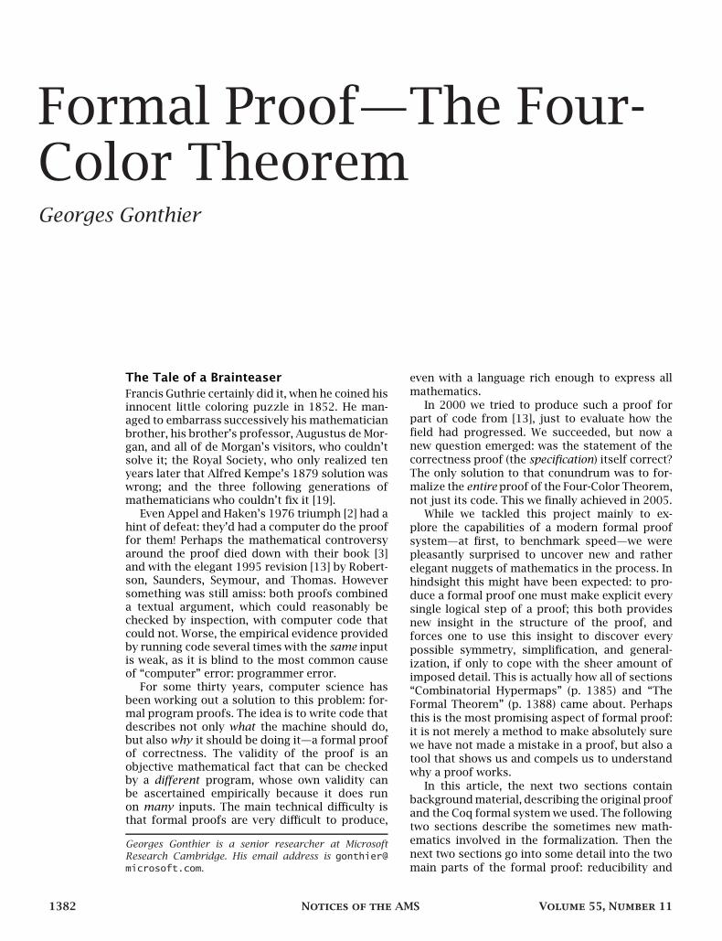
map must contain an n-gon with n < 6, i.e., one of

the following map fragments.

Each such configuration consists of a completekernel face surrounded by a ring of partial faces.

Erasing an edge of a digon or triangle yields asmaller map, which is four-colorable by induction.This coloring uses at most three colors for thering, leaving us a free color for the kernel face,so the original map is also four-colorable. Erasingan appropriate pair of opposite edges disposes ofthe square configuration similarly.

In the pentagon case, however, it is necessaryto modify the inductive coloring to free a ringcolor for the kernel face. Kempe tried to do this bylocally inverting the colors inside a two-toned max-imal contiguous group of faces (a “Kempe chain”).By planarity, chains cannot cross, and Kempeenumerated their arrangements and showed thatconsecutive inversions freed a ring color. Alas, it isnot always possible to do consecutive inversions,as inverting one chain can scramble other chains.It took ten years to spot this error and almost acentury to fix it.

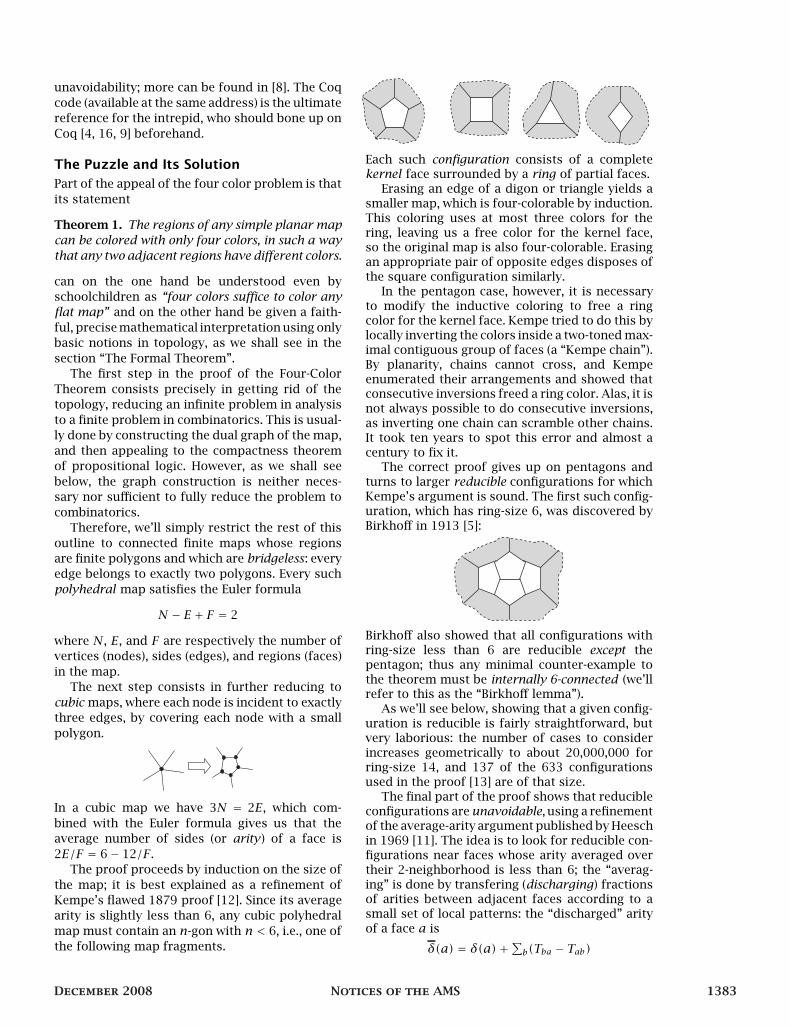
The correct proof gives up on pentagons andturns to larger reducible configurations for whichKempe’s argument is sound. The first such config-uration, which has ring-size 6, was discovered byBirkhoff in 1913 [5]:

Birkhoff also showed that all configurations withring-size less than 6 are reducible except thepentagon; thus any minimal counter-example tothe theorem must be internally 6-connected (we’llrefer to this as the “Birkhoff lemma”).

As we’ll see below, showing that a given config-uration is reducible is fairly straightforward, butvery laborious: the number of cases to considerincreases geometrically to about 20,000,000 forring-size 14, and 137 of the 633 configurationsused in the proof [13] are of that size.

The final part of the proof shows that reducibleconfigurations are unavoidable, using a refinementof the average-arity argument published by Heeschin 1969 [11]. The idea is to look for reducible con-figurations near faces whose arity averaged overtheir 2-neighborhood is less than 6; the “averag-ing” is done by transfering (discharging) fractionsof arities between adjacent faces according to asmall set of local patterns: the “discharged” arityof a face a is

δ(a) = δ(a)+∑b(Tba − Tab)

December 2008 Notices of the AMS 1383

where δ(a) is the original arity of a, and Tba is thearity fraction transfered from b. Thus the averagedischarged arity remains 6− 12/F < 6.

The proof enumerates all internally 6-connected2-neighborhoods whose discharged arity is lessthan 6. This enumeration is fairly complex, butnot as computationally intensive as the reducibil-ity checks: the search is heavily constrainedas the neighborhoods consist of two disjointconcentric rings of 5+-gons. Indeed in [13] re-ducible configurations are always found inside the2-neighborhoods, and the central face is a 7+-gon.

Coq and the Calculus of InductiveConstructions

The Coq formal proof system (or assistant ) [4,16], which we used for our work is based ona version of higher-order logic, the Calculus ofinductive Constructions (CiC) [6] whose specificfeatures—propositions as types, dependent types,and reflection—all played an important part in thesuccess of our project.

We have good reason to leave the familiar,dead-simple world of untyped first-order logic forthe more exotic territory of Type Theory [10, 4]. Infirst-order logic, higher-level (“meta”) argumentsare second-class citizens: they are interpreted asinformal procedures that should be expandedout to primitive inferences to achieve full rigor.This is fine in a non-formal proof, but rapidlybecomes impractical in a formal one because oframping complexity. Computer automation canmitigate this, but type theory supplies a muchmore satisfactory solution, levelling the playingfield by providing a language that can expressmeta-arguments.

This can indeed be observed even with thesimplest first-order type system. Consider thecommutativity of integer addition,

∀x, y ∈ N, x+ y = y + x

There are two hidden premises, x ∈ N and y ∈ N,that need to be verified separately every time thelaw is used. This seems innocuous enough, exceptx and y may be replaced by huge expressions forwhich the x, y ∈ N premises are not obvious, evenfor machine automation. By contrast, the typedversion of commutativity

∀x, y : Nat, x+ y = y + x

can be applied to any expression A + B withoutfurther checks, because the premises follow fromthe way A and B are written. We are simply notallowed to write drivel such as 1+ true, and conse-quently we don’t need to worry about its existence,even in a fully formal proof—we have “proof bynotation”.

Our formal proof uses this, and much more:proof types, dependent types, and reflection, aswe will now explain.

Proof types are types that encode logic (they’re

also called “propositions-as-types”). The encod-ing exploits a strong similarity between type andlogic rules, which is most apparent when both

are written in natural deduction style (see [10] inthis issue), e.g., consider function application andmodus ponens (MP):

f : A→ B x : A

f x : B

A⇒ B A

B

The rules are identical if one ignores the terms tothe left of “:”. However these terms can also beincluded in the correspondence, by interpretingx : A and “x proves A” rather than “x is of type A”.

In the above we have that f x proves B becausex proves A and f proves A ⇒ B, so the applica-tion f x on the left denotes the MP deduction on

the right. This holds in general: proof types areinhabited by proof objects.

CiC is entirely based on this correspondence,

which goes back to Curry and Howard. CiC is aformalism without a formal logic, a sensible sim-plification: as we’ve argued we need types anyway,

so why add a redundant logic? The availabilityof proof objects has consequences both for ro-bustness, as they provide a practical means of

storing and thus independently checking proofs,and for expressiveness, as they let us describeand prove algorithms that create and processproofs—meta-arguments.

The correspondence in CiC is not limited toHerbrand term and minimal logic; it interpretsmost data and programming constructs common

in computer science as useful logical connectivesand deduction rules, e.g., pairs as “and”

x : A y : B

〈x, y〉 : A× B

u : A× B

u.1 : A u.2 : B

A B

A∧ B

A∧ B

A B

tagged unions as “or”, conditional (if-then-else)as proof by cases, recursive definitions as proofby induction, and so on. The correspondence

even works backwards for the logical rule ofgeneralization: we have

Γ ⊢ B[x] x not free in ΓΓ ⊢ ∀x, B[x])

Γ , x : A ⊢ t[x] : B[x]

Γ ⊢ (fun x : A֏ t[x]) : (∀x : A,B[x])

The proof/typing context Γ is explicit here becauseof the side condition. Generalization is interpret-ed by a new, stronger form of function definition

that lets the type of the result depend on a for-mal parameter. Note that the nondependent caseinterprets the Deduction Theorem.

The combination of these dependent types withproof types leads to the last feature of CiC we wish


to highlight in this section, computational reflec-

tion. Because of dependent types, data, functions

and therefore (potential) computation can appear

in types. The normal mathematical practice is

to interpret such meta-data, replacing a constant

by its definition, instantiating formal parameters,

selecting a case, etc. CiC supports this through

a typing rule that lets such computation happen

transparently:

t : A A ≡βιδζ B

t : B

This rule states that the βιδζ-computation rules

of CiC yield equivalent types. It is a subsumption

rule: there is no record of its use in the proof

term t . Aribitrary long computations can thus

be elided from a proof, as CiC has an ι-rule for

recursion.

This yields an entirely new way of proving

results about specific calculations: computing!

Henri Poincaré once pointed out that one does

not “prove” 2 + 2 = 4, one “checks” it. CiC can

do just that: if erefl : ∀x, x = x is the reflexivity

axiom, and the constants +, 2, 4 denote a recursive

function that computes integer addition, and the

representation of the integers 2 and 4, respective-

ly, then erefl 4 proves 2+2 = 4 because 2+2 = 4

and 4 = 4 are just different denotations of the

same proposition.

While the Poincaré example is trivial, we would

probably not have completed our proof with-

out computational reflection. At the heart of the

reducibility proof, we define

Definition check_reducible cf : bool := ...

Definition cfreducible cf : Prop :=

c_reducible (cfring cf) (cfcontract cf).

where check_reducible cf calls a complex

reducibility decision procedure that works on

a specific encoding of configurations, while

c_reducible r c is a logical predicate that as-

serts the reducibility of a configuration map with

ring r and deleted edges (contract) c; cfring cf

denotes the ring of the map represented by cf.

We then prove

Lemma check_reducible_valid :

forall cf : config,

check_reducible cf = true -> cfreducible cf.

This is the formal partial correctness proof of

the decision procedure; it’s large, but nowhere

near the size of an explicit reducibility proof.

With the groundwork done, all reducibility proofs

become trivial, e.g.,

Lemma cfred232 : cfreducible (Config 11 33 37

H 2 H 13 Y 5 H 10 H 1 H 1 Y 3 H 11 Y 4 H 9

H 1 Y 3 H 9 Y 6 Y 1 Y 1 Y 3 Y 1 Y Y 1 Y).

Proof.

apply check_reducible_valid.

vm_compute; reflexivity.

Qed.

In CiC, this 20,000,000-cases proof, is almost astrivial as the Poincaré 2 + 2 = 4: apply the cor-rectness lemma, then reflexivity up to (a big!)computation. Note that we make essential useof dependent and proof types, as the cubic mapcomputed by cfring is passed implicitly insidethe type of the returned ring. cfring mediatesbetween a string representation of configurations,well suited to algorithms, and a more mathemat-ical one, better suited for abstract graph theory,which we shall describe in the next section.

Combinatorial Hypermaps

Although the Four-Color Theorem is superficiallystated in analysis, it really is a result in com-binatorics, so common sense suggests that thebulk of the proof should use solely combinatorialstructure. Oddly, most accounts of the proof usegraphs homeomorphically embedded in the planeor sphere, dragging analysis into the combina-torics. This does allow appealing to the JordanCurve Theorem in a pinch, but this is hardly help-ful if one does not already have the Jordan CurveTheorem in store.

Moreover, graphs lack the data to do geometrictraversals, e.g., traversing the first neighborhoodof a face in clockwise order; it is necessary to goback to the embedding to recover this informa-tion. This will not be easy in a fully formal proof,where one does not have the luxury of appealingto pictures or “folklore” when cornered.

The solution to this problem is simply to addthe missing data. This yields an elegant and highlysymmetrical structure, the combinatorial hyper-map [7, 17].

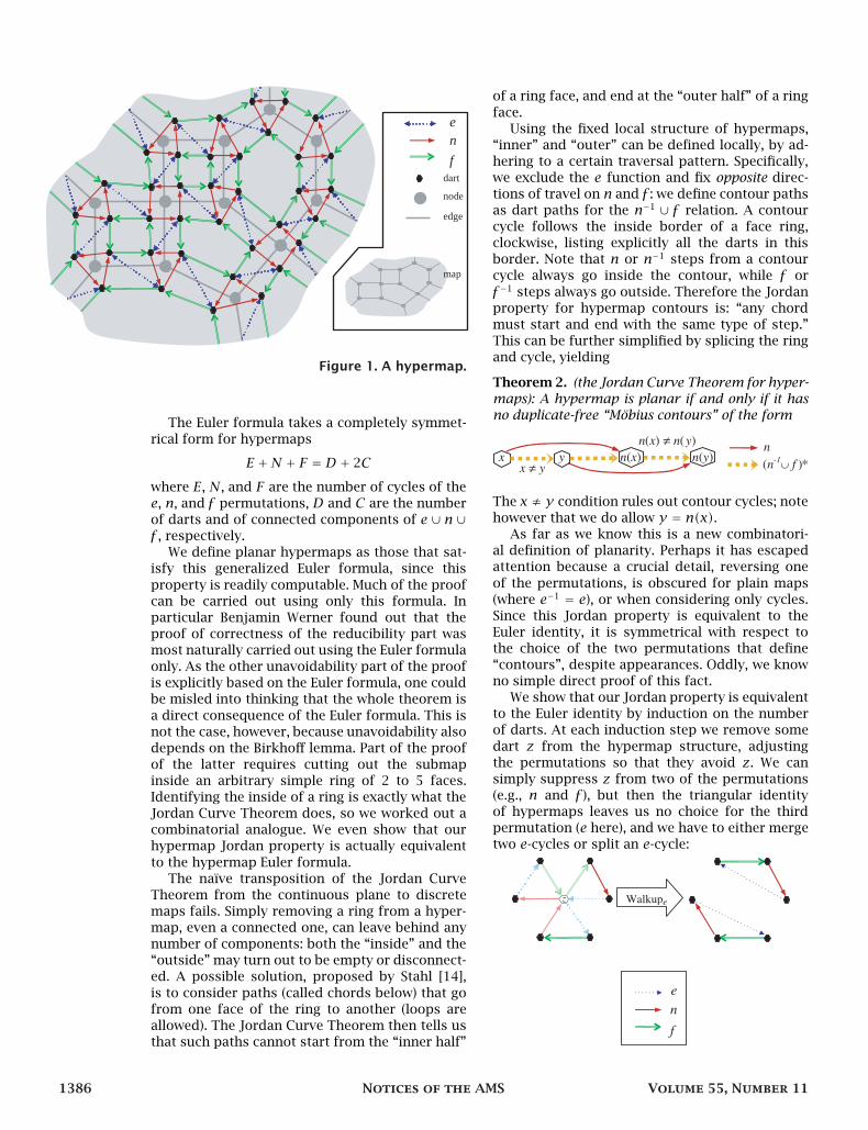
Definition 1. A hypermap is a triple of functions〈e, n, f 〉 on a finite set d of darts that satisfy thetriangular identity e ◦ n ◦ f = 1.

Note the circular symmetry of the identity: 〈n, f , e〉and 〈f , e, n〉 are also hypermaps. Obviously, thecondition forces all the functions to be permu-tations of d, and fixing any two will determinethe third; indeed hypermaps are often definedthis way. We choose to go with symmetry instead,because this lets us use our constructions and the-orems three times over. The symmetry also clearlydemonstrates that the dual graph constructionplays no part in the proof.

We have found that the relation between hyper-maps and “plain” polyhedral maps is best depictedby drawing darts as points placed at the cornersof the polygonal faces, and using arrows for thethree functions, with the cycles of the f func-tion going counter-clockwise inside each face, andthose of the n function around each node. On aplain map each edge has exactly two endpoints,and consequently each e cycle is a double-endedarrow cutting diagonally across the n − f − n − frectangle that straddles an edge (Figure 1).


e n

f dart

node

edge

map

Figure 1. A hypermap.

The Euler formula takes a completely symmet-

rical form for hypermaps

E +N + F = D + 2C

where E, N, and F are the number of cycles of the

e, n, and f permutations, D and C are the number

of darts and of connected components of e ∪ n∪f , respectively.

We define planar hypermaps as those that sat-

isfy this generalized Euler formula, since this

property is readily computable. Much of the proof

can be carried out using only this formula. In

particular Benjamin Werner found out that the

proof of correctness of the reducibility part was

most naturally carried out using the Euler formula

only. As the other unavoidability part of the proof

is explicitly based on the Euler formula, one could

be misled into thinking that the whole theorem is

a direct consequence of the Euler formula. This is

not the case, however, because unavoidability also

depends on the Birkhoff lemma. Part of the proof

of the latter requires cutting out the submap

inside an arbitrary simple ring of 2 to 5 faces.

Identifying the inside of a ring is exactly what the

Jordan Curve Theorem does, so we worked out a

combinatorial analogue. We even show that our

hypermap Jordan property is actually equivalent

to the hypermap Euler formula.

The naïve transposition of the Jordan Curve

Theorem from the continuous plane to discrete

maps fails. Simply removing a ring from a hyper-

map, even a connected one, can leave behind any

number of components: both the “inside” and the

“outside” may turn out to be empty or disconnect-

ed. A possible solution, proposed by Stahl [14],

is to consider paths (called chords below) that go

from one face of the ring to another (loops are

allowed). The Jordan Curve Theorem then tells us

that such paths cannot start from the “inner half”

of a ring face, and end at the “outer half” of a ring

face.

Using the fixed local structure of hypermaps,

“inner” and “outer” can be defined locally, by ad-

hering to a certain traversal pattern. Specifically,

we exclude the e function and fix opposite direc-

tions of travel on n and f : we define contour paths

as dart paths for the n−1 ∪ f relation. A contour

cycle follows the inside border of a face ring,

clockwise, listing explicitly all the darts in this

border. Note that n or n−1 steps from a contour

cycle always go inside the contour, while f or

f−1 steps always go outside. Therefore the Jordan

property for hypermap contours is: “any chord

must start and end with the same type of step.”

This can be further simplified by splicing the ring

and cycle, yielding

Theorem 2. (the Jordan Curve Theorem for hyper-

maps): A hypermap is planar if and only if it has

no duplicate-free “Möbius contours” of the form

The x ≠ y condition rules out contour cycles; note

however that we do allow y = n(x).As far as we know this is a new combinatori-

al definition of planarity. Perhaps it has escaped

attention because a crucial detail, reversing one

of the permutations, is obscured for plain maps

(where e−1 = e), or when considering only cycles.

Since this Jordan property is equivalent to the

Euler identity, it is symmetrical with respect to

the choice of the two permutations that define

“contours”, despite appearances. Oddly, we know

no simple direct proof of this fact.

We show that our Jordan property is equivalent

to the Euler identity by induction on the number

of darts. At each induction step we remove some

dart z from the hypermap structure, adjusting

the permutations so that they avoid z. We can

simply suppress z from two of the permutations

(e.g., n and f ), but then the triangular identity

of hypermaps leaves us no choice for the third

permutation (e here), and we have to either merge

two e-cycles or split an e-cycle:

e

n

f

z Walkupe


pat ch

disk

remainde r

c ontour cy cle

full m ap

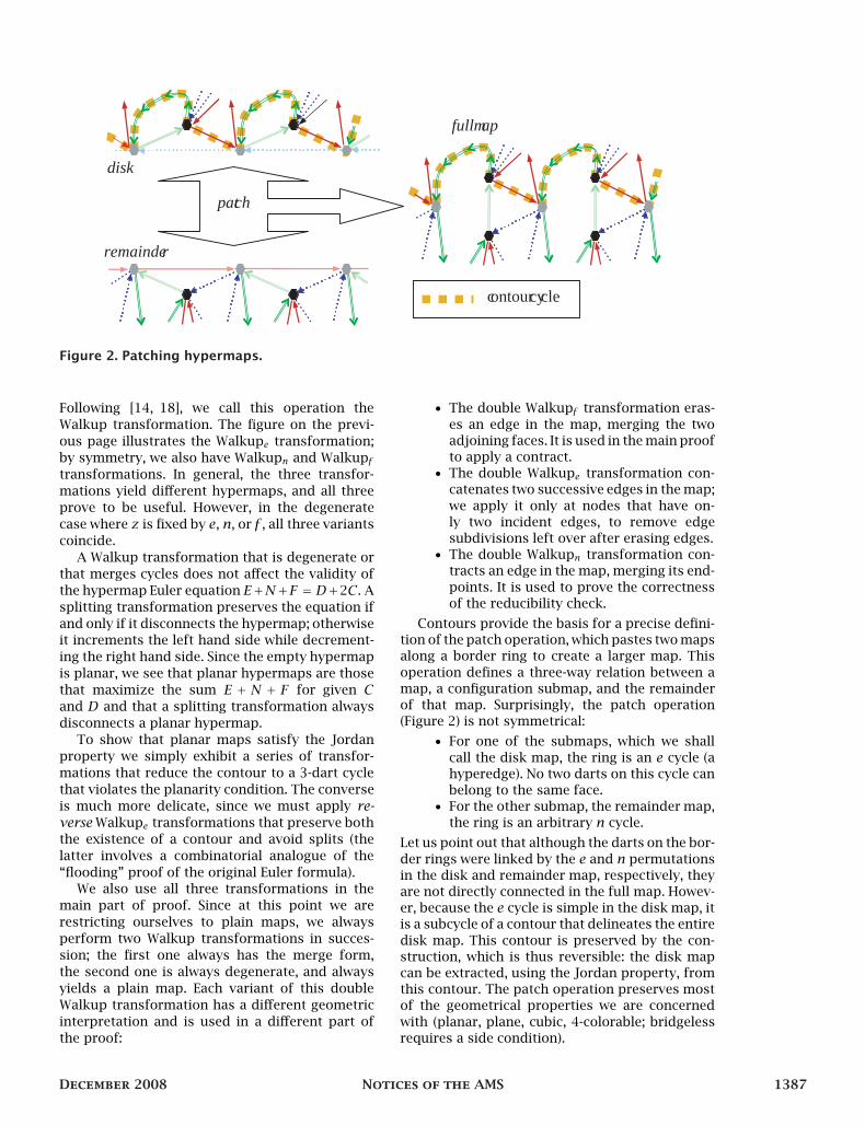
Figure 2. Patching hypermaps.

Following [14, 18], we call this operation the

Walkup transformation. The figure on the previ-

ous page illustrates the Walkupe transformation;

by symmetry, we also have Walkupn and Walkupftransformations. In general, the three transfor-

mations yield different hypermaps, and all three

prove to be useful. However, in the degenerate

case where z is fixed by e, n, or f , all three variants

coincide.

A Walkup transformation that is degenerate or

that merges cycles does not affect the validity of

the hypermap Euler equation E+N+F = D+2C. A

splitting transformation preserves the equation if

and only if it disconnects the hypermap; otherwise

it increments the left hand side while decrement-

ing the right hand side. Since the empty hypermap

is planar, we see that planar hypermaps are those

that maximize the sum E + N + F for given C

and D and that a splitting transformation always

disconnects a planar hypermap.

To show that planar maps satisfy the Jordan

property we simply exhibit a series of transfor-

mations that reduce the contour to a 3-dart cycle

that violates the planarity condition. The converse

is much more delicate, since we must apply re-

verse Walkupe transformations that preserve both

the existence of a contour and avoid splits (the

latter involves a combinatorial analogue of the

“flooding” proof of the original Euler formula).

We also use all three transformations in the

main part of proof. Since at this point we are

restricting ourselves to plain maps, we always

perform two Walkup transformations in succes-

sion; the first one always has the merge form,

the second one is always degenerate, and always

yields a plain map. Each variant of this double

Walkup transformation has a different geometric

interpretation and is used in a different part of

the proof:

• The double Walkupf transformation eras-

es an edge in the map, merging the two

adjoining faces. It is used in the main proof

to apply a contract.

• The double Walkupe transformation con-

catenates two successive edges in the map;

we apply it only at nodes that have on-

ly two incident edges, to remove edge

subdivisions left over after erasing edges.

• The double Walkupn transformation con-

tracts an edge in the map, merging its end-

points. It is used to prove the correctness

of the reducibility check.

Contours provide the basis for a precise defini-

tion of the patch operation, which pastes two maps

along a border ring to create a larger map. This

operation defines a three-way relation between a

map, a configuration submap, and the remainder

of that map. Surprisingly, the patch operation

(Figure 2) is not symmetrical:

• For one of the submaps, which we shall

call the disk map, the ring is an e cycle (a

hyperedge). No two darts on this cycle can

belong to the same face.

• For the other submap, the remainder map,

the ring is an arbitrary n cycle.

Let us point out that although the darts on the bor-

der rings were linked by the e and n permutations

in the disk and remainder map, respectively, they

are not directly connected in the full map. Howev-

er, because the e cycle is simple in the disk map, it

is a subcycle of a contour that delineates the entire

disk map. This contour is preserved by the con-

struction, which is thus reversible: the disk map

can be extracted, using the Jordan property, from

this contour. The patch operation preserves most

of the geometrical properties we are concerned

with (planar, plane, cubic, 4-colorable; bridgeless

requires a side condition).


Step 1 St eps 2- 3 St ep 4

St eps 6- 7 Step 5 St ep 8

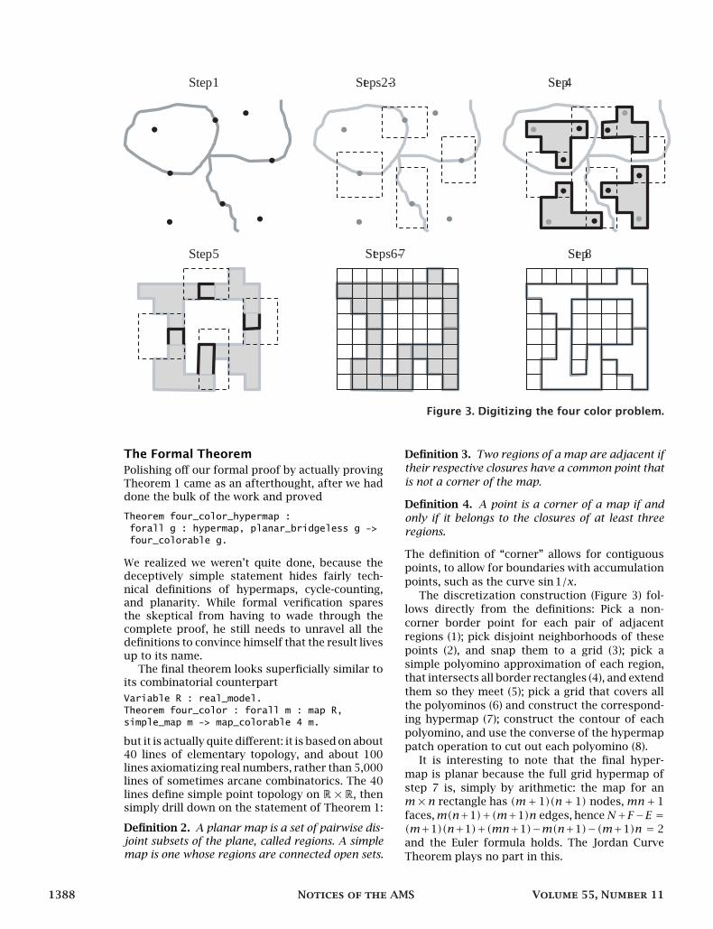
Figure 3. Digitizing the four color problem.

The Formal Theorem

Polishing off our formal proof by actually proving

Theorem 1 came as an afterthought, after we haddone the bulk of the work and proved

Theorem four_color_hypermap :

forall g : hypermap, planar_bridgeless g ->

four_colorable g.

We realized we weren’t quite done, because thedeceptively simple statement hides fairly tech-nical definitions of hypermaps, cycle-counting,and planarity. While formal verification sparesthe skeptical from having to wade through thecomplete proof, he still needs to unravel all thedefinitions to convince himself that the result lives

up to its name.The final theorem looks superficially similar to

its combinatorial counterpart

Variable R : real_model.

Theorem four_color : forall m : map R,

simple_map m -> map_colorable 4 m.

but it is actually quite different: it is based on about40 lines of elementary topology, and about 100lines axiomatizing real numbers, rather than 5,000lines of sometimes arcane combinatorics. The 40

lines define simple point topology on R×R, thensimply drill down on the statement of Theorem 1:

Definition 2. A planar map is a set of pairwise dis-joint subsets of the plane, called regions. A simplemap is one whose regions are connected open sets.

Definition 3. Two regions of a map are adjacent if

their respective closures have a common point that

is not a corner of the map.

Definition 4. A point is a corner of a map if and

only if it belongs to the closures of at least three

regions.

The definition of “corner” allows for contiguous

points, to allow for boundaries with accumulation

points, such as the curve sin 1/x.

The discretization construction (Figure 3) fol-

lows directly from the definitions: Pick a non-

corner border point for each pair of adjacent

regions (1); pick disjoint neighborhoods of these

points (2), and snap them to a grid (3); pick a

simple polyomino approximation of each region,

that intersects all border rectangles (4), and extend

them so they meet (5); pick a grid that covers all

the polyominos (6) and construct the correspond-

ing hypermap (7); construct the contour of each

polyomino, and use the converse of the hypermap

patch operation to cut out each polyomino (8).

It is interesting to note that the final hyper-

map is planar because the full grid hypermap of

step 7 is, simply by arithmetic: the map for an

m×n rectangle has (m+ 1)(n+ 1) nodes,mn+ 1

faces,m(n+1)+(m+1)n edges, henceN+F−E =

(m+1)(n+1)+(mn+1)−m(n+1)−(m+1)n = 2

and the Euler formula holds. The Jordan Curve

Theorem plays no part in this.


Checking Reducibility

Although reducibility is quite demanding compu-

tationally, it also turned out to be the easiest part

of the proof to formalize. Even though we used

more sophisticated algorithms, e.g., multiway de-

cision diagrams (MDDs) [1], this part of the formal

proof was completed in a few part-time months.

By comparison, the graph theory in section “Com-

binatorial Hypermaps” (p. 1385) took a few years

to sort out.

The reducibility computation consists in iter-

ating a formalized version of the Kempe chain

argument, in order to compute a lower bound for

the set of colorings that can be “fitted” to match a

coloring of the configuration border, using color

swaps. Each configuration comes with a set of

one to four edges, its contract [13], and the actual

check verifies that the lower bound contains all the

colorings of the contract map obtained by erasing

the edges of contract.

The computation keeps track of both ring col-

orings and arrangement of Kempe chains. To cut

down on symmetries, their representation uses

the fact that four-coloring the faces of a cubic

map is equivalent to three-coloring its edges; this

result goes back Tait in 1880 [15]. Thus a coloring

is represented by a word on the alphabet {1,2,3}.

Kempe inversions for edge colorings amount to

inverting the edge colors along a two-toned path

(a chain) incident to ring edges. Since the map is

cubic the chains for any given pair of colors (say

2 and 3) are always disjoint and thus define an

outerplanar graph, which is readily represented

by a bracket (or Dyck) word on a 4-letter alphabet:

traversing the ring edges counterclockwise, write

down

• a • if the edge is not part of a chain because

it has color 1

• a [ if the edge starts a new chain

• a ]0 (resp. ]1) if the edge is the end of a

chain of odd (resp. even) length

As the chain graph is outerplanar, brackets for

the endpoints of any chain match. We call such a

four-letter word a chromogram.

Since we can flip simultaneously any subset of

the chains, a given chromogram will match any

ring coloring that assigns color 1 to • edges and

those only, and assigns different colors to edges

with matching brackets if and only if the closing

bracket is a ]1. We say that such a coloring is

consistent with the chromogram.

Let us say that a ring coloring of the remainder

map is suitable if it can be transformed, via a

sequence alternating chain inversions and a cyclic

permutation ρ of {1,2,3}, into a ring coloring of

the configuration. A configuration will thus be re-

ducible when all the ring colorings of its contract

map are suitable. The reducibility check consists

in computing an upper bound of the set of non-

suitable colorings and checking that it is disjointfrom the set of contract colorings.

The upper bound is the limit of a decreasingsequence Ξ0, . . . ,Ξi , . . . starting with the set Ξ0 ofall valid colorings; we simultaneously compute

upper bounds Λ0, . . . ,Λi, . . . of the set of chromo-grams not consistent with any suitable coloring.Each iteration starts with a set ∆Θi of suitable

colorings, taking the set of ring colorings of theconfiguration for ∆Θ0.

(1) We get Λi+1 by removing all chromogramsconsistent with some θ ∈ ∆Θi from Λi

(2) We remove from Ξi all colorings ξ that arenot consistent with any λ ∈ Λi+1; this issound since any coloring that induces ξwill also induce a chromogramγ ∉ Λi+1. Asγ is consistent with both ξ and a suitable

coloring θ, there exists a chain inversionthat transforms ξ into θ.

(3) Finally we get ∆Θi+1 by applying ρ and ρ−1

to the colorings that were deleted from Ξi ;we stop if there were none.

We use 3- and 4-way decision diagrams to repre-sent the various sets: a {1,2,3} edge-labeled treerepresents a set of colorings, and a {•, [, ]0, ]1}

edge-labeled tree represents a set of chromo-grams. In the MDD for Ξi , the leaf reached by

following the branch labeled with some ξ ∈ Ξistores the number of matching λ ∈ Λi , so thatstep 2 is in amortized constant time (each consis-

tent pair is considered at most twice); the MDDstructures are optimized in several other ways.

The correctness proof consists in showing that

the optimized MDD structure computes the rightsets, mainly by stepping through the functions,

and in showing the existence of the chromogramγ in step 2 above. Following a suggestion byB. Werner, we do this with a single induction on

the remainder map, without developing any ofthe informal justification of the procedure: in thiscase, the formal proof turns out to be simpler than

the informal proof that inspired it!The 633 configuration maps are the only link

between the reducibility check and the main proof.A little analysis reveals that each of these mapscan be built inside-out from a simple construction

program. We cast all the operations we need, suchas computing the set of colorings, the contractmap, or even compiling an occurrence check filter,

as nonstandard interpretations of this program(the standard one being the map construction).

This approach affords both efficient implementa-tion and straightforward correctness proofs basedon simulation relations between the standard and

nonstandard interpretations.The standard interpretation yields a pointed

remainder map, i.e., a plain map with a distin-

guished dart x which is cubic except for the cycle


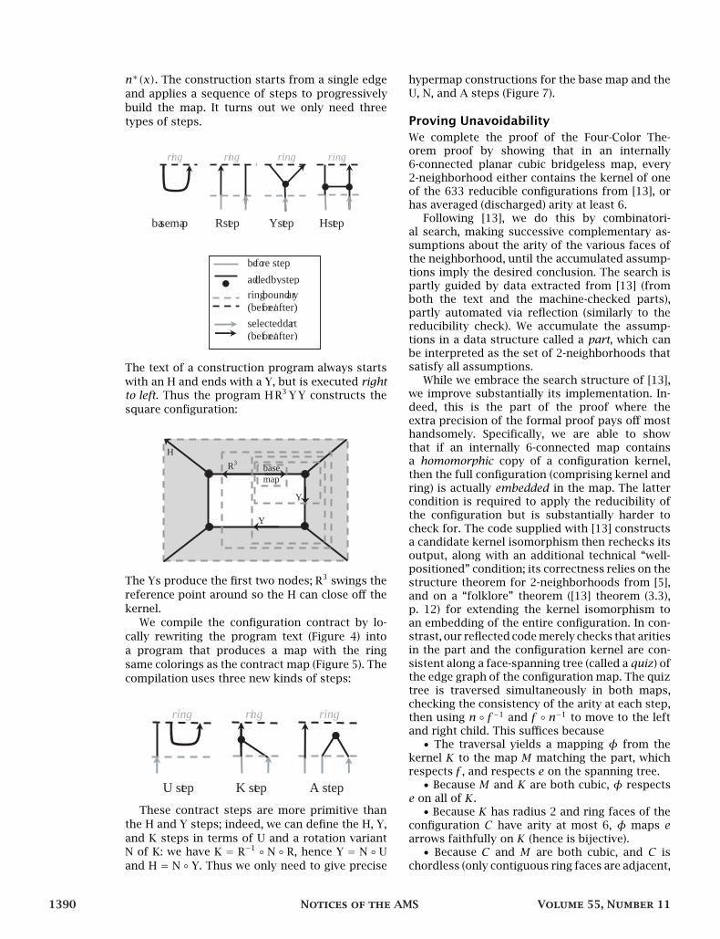
n∗(x). The construction starts from a single edge

and applies a sequence of steps to progressively

build the map. It turns out we only need three

types of steps.

ba se ma p

ri ng ring

Y st ep

ring

H st ep

be fo re step

ad ded by step ring bound ar y (bef or e/ after)

selected da rt (bef or e/ after)

ri ng

R st ep

The text of a construction program always starts

with an H and ends with a Y, but is executed right

to left. Thus the program H R3 Y Y constructs the

square configuration:

R 3

H

Y

Y

base map

The Ys produce the first two nodes; R3 swings the

reference point around so the H can close off the

kernel.

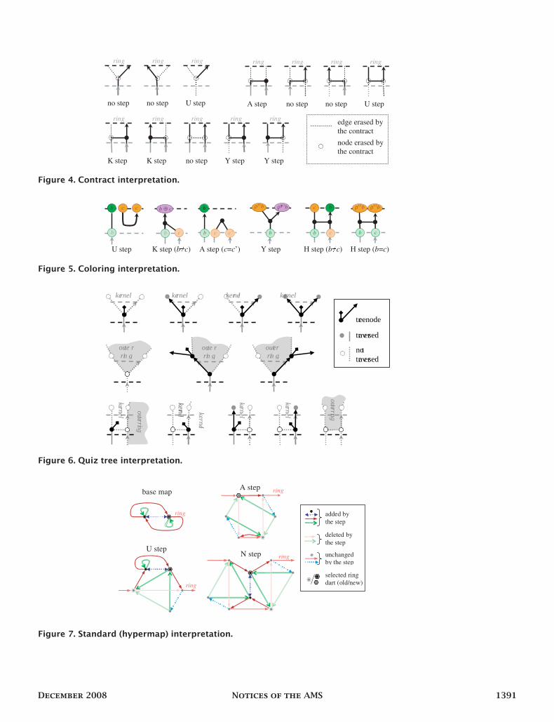
We compile the configuration contract by lo-

cally rewriting the program text (Figure 4) into

a program that produces a map with the ring

same colorings as the contract map (Figure 5). The

compilation uses three new kinds of steps:

U st ep

ring ring

A step

ri ng

K st ep

These contract steps are more primitive than

the H and Y steps; indeed, we can define the H, Y,

and K steps in terms of U and a rotation variant

N of K: we have K = R−1 ◦ N ◦ R, hence Y = N ◦ U

and H = N ◦ Y. Thus we only need to give precise

hypermap constructions for the base map and the

U, N, and A steps (Figure 7).

Proving Unavoidability

We complete the proof of the Four-Color The-orem proof by showing that in an internally

6-connected planar cubic bridgeless map, every

2-neighborhood either contains the kernel of oneof the 633 reducible configurations from [13], or

has averaged (discharged) arity at least 6.Following [13], we do this by combinatori-

al search, making successive complementary as-

sumptions about the arity of the various faces ofthe neighborhood, until the accumulated assump-

tions imply the desired conclusion. The search is

partly guided by data extracted from [13] (fromboth the text and the machine-checked parts),

partly automated via reflection (similarly to thereducibility check). We accumulate the assump-

tions in a data structure called a part, which can

be interpreted as the set of 2-neighborhoods thatsatisfy all assumptions.

While we embrace the search structure of [13],we improve substantially its implementation. In-

deed, this is the part of the proof where the

extra precision of the formal proof pays off mosthandsomely. Specifically, we are able to show

that if an internally 6-connected map containsa homomorphic copy of a configuration kernel,

then the full configuration (comprising kernel and

ring) is actually embedded in the map. The lattercondition is required to apply the reducibility of

the configuration but is substantially harder to

check for. The code supplied with [13] constructsa candidate kernel isomorphism then rechecks its

output, along with an additional technical “well-positioned” condition; its correctness relies on the

structure theorem for 2-neighborhoods from [5],

and on a “folklore” theorem ([13] theorem (3.3),p. 12) for extending the kernel isomorphism to

an embedding of the entire configuration. In con-strast, our reflected code merely checks that arities

in the part and the configuration kernel are con-

sistent along a face-spanning tree (called a quiz) ofthe edge graph of the configuration map. The quiz

tree is traversed simultaneously in both maps,

checking the consistency of the arity at each step,then using n ◦ f−1 and f ◦ n−1 to move to the left

and right child. This suffices because• The traversal yields a mapping φ from the

kernel K to the map M matching the part, which

respects f , and respects e on the spanning tree.• Because M and K are both cubic, φ respects

e on all of K.• Because K has radius 2 and ring faces of the

configuration C have arity at most 6, φ maps earrows faithfully on K (hence is bijective).• Because C and M are both cubic, and C is

chordless (only contiguous ring faces are adjacent,


ri ng

U st ep

ri ng

no step

ri ng

no step

ri ng

no step

ri ng

K st ep

ri ng

K st ep

ri ng

Y st ep

ri ng

Y st ep

ri ng

A st ep

ri ng

no step

ri ng

no step

ri ng

U step

ed ge erased by

the co ntra ct

node er as ed by

the co ntra ct

Figure 4. Contract interpretation.

b

b c c

b

b

c

c

b

b

c c’

b ⊕ c

b c b

ρ 1 b ρ ±1 b

U step K st ep ( b c ) A step ( c = c ’) Y step H st ep ( b c ) H st ep ( b = c )

b c

ρ ±1 b ρ ±1 b

Figure 5. Coloring interpretation.

out er ri n g

ou te r ri n g

ou te r ri n g

ou te r ri ng

ou te r ri ng

kerne l

ker ne l

ke rnel

ke rnel

ke rnel

ker ne l

ke rnel ke rnel ker ne l ke rnel

tr av er sed

no t tr av er sed

tr ee node

Figure 6. Quiz tree interpretation.

base map

U step N step

A step

ring

ring

ring

ring

added by

the step

deleted by

the step

unchanged

by the step

selected ring

dart (old/new)

Figure 7. Standard (hypermap) interpretation.


u l

u r

u r

u l

u u

h

h l

h r

f 1 l

f 1 r

f 1 l

f 0 r

f 2 l

u

h

f 2 r

f 0 l

f 0 r

hub spoke

spoke

spoke hat

hat fan

fa n

le ft qu iz step

ri gh t qu iz st ep

subp art da rts

un reachable da rt

spoke

u l u r

h l h r

Figure 8. The hypermap of a subpart.

because each has arity at least 3), φ extends to an

embedding of C in M .

The last three assertions are proved by induc-

tion over the size of the disk map of a contour

containing a counter-example edge. For the third

assertion, the contour is inM and spans at most 5

faces because it is the image of a simple non-cyclic

path in K. Its interior must be empty for otherwise

it would have to be a single pentagon (because Mis internally 6-connected) that would be the image

of a ring face adjacent to 5 kernel and 2 ring faces,

contrary to the arity constraint.

We check the radius and arity conditions explic-

itly for each configuration, along with the sparsity

and triad conditions on its contract [13]; the ring

arity conditions are new to our proof. The checks

and the quiz tree selection are formulated as non-

standard interpretations; the quiz interpretation

(Figure 6) runs programs left-to-right, backwards.

Because our proof depends only on the Birkhoff

lemma (which incidentally we prove by reflection

using a variant of the reducibility check), we do

not need “cartwheels” as in [13] to represent

2-neighborhoods; the unavoidability check uses

only “parts” and “quizzes”. We also use parts to

represent the arity discharging rules, using func-

tions that intersect, rotate, and reflect (mirror)

parts, e.g., a discharging rule applies to a part P if

and only if its part subsumes P .

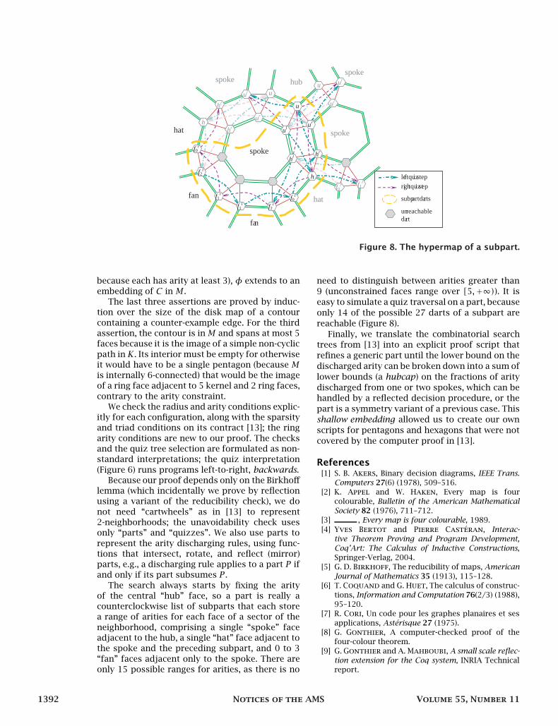
The search always starts by fixing the arity

of the central “hub” face, so a part is really a

counterclockwise list of subparts that each store

a range of arities for each face of a sector of the

neighborhood, comprising a single “spoke” face

adjacent to the hub, a single “hat” face adjacent to

the spoke and the preceding subpart, and 0 to 3

“fan” faces adjacent only to the spoke. There are

only 15 possible ranges for arities, as there is no

need to distinguish between arities greater than

9 (unconstrained faces range over [5,+∞)). It is

easy to simulate a quiz traversal on a part, because

only 14 of the possible 27 darts of a subpart are

reachable (Figure 8).

Finally, we translate the combinatorial search

trees from [13] into an explicit proof script that

refines a generic part until the lower bound on the

discharged arity can be broken down into a sum of

lower bounds (a hubcap) on the fractions of arity

discharged from one or two spokes, which can be

handled by a reflected decision procedure, or the

part is a symmetry variant of a previous case. This

shallow embedding allowed us to create our own

scripts for pentagons and hexagons that were not

covered by the computer proof in [13].

References[1] S. B. Akers, Binary decision diagrams, IEEE Trans.

Computers 27(6) (1978), 509–516.

[2] K. Appel and W. Haken, Every map is four

colourable, Bulletin of the American Mathematical

Society 82 (1976), 711–712.

[3] , Every map is four colourable, 1989.

[4] Yves Bertot and Pierre Castéran, Interac-

tive Theorem Proving and Program Development,

Coq’Art: The Calculus of Inductive Constructions,

Springer-Verlag, 2004.

[5] G. D. Birkhoff, The reducibility of maps, American

Journal of Mathematics 35 (1913), 115–128.

[6] T. Coquand and G. Huet, The calculus of construc-

tions, Information and Computation 76(2/3) (1988),

95–120.

[7] R. Cori, Un code pour les graphes planaires et ses

applications, Astérisque 27 (1975).

[8] G. Gonthier, A computer-checked proof of the

four-colour theorem.

[9] G. Gonthier and A. Mahboubi, A small scale reflec-

tion extension for the Coq system, INRIA Technical

report.


[10] T. Hales, Formal proofs, Notices of the AMS, this

issue.

[11] H. Heesch, Untersuchungen zum Vierfarbenprob-

lem, 1969.

[12] A. B. Kempe, On the geographical problem of the

four colours, American Journal of Mathematics 2(3)

(1879), 193–200.

[13] N. Robertson, D. Sanders, P. Seymour, and

R. Thomas, The four-colour theorem, J. Combina-

torial Theory, Series B 70 (1997), 2–44.

[14] S. Stahl, A combinatorial analog of the Jordan

curve theorem, J. Combinatorial Theory, Series B 35

(1983), 28–38.

[15] P. G. Tait, Note on a theorem in the geometry of po-

sition, Trans. Royal Society of Edinburgh 29 (1880),

657–660.

[16] The Coq development team, The Coq Proof Assistant

Reference Manual, version 8.1, 2006.

[17] W. T. Tutte, Duality and trinity, Colloquium

Mathematical Society Janos Bolyai 10 (1975),

1459–1472.

[18] D. W. Walkup, How many ways can a permutation

be factored into two n-cycles?, Discrete Mathematics

28 (1979), 315–319.

[19] R. Wilson, Four Colours Suffice, Allen Lane Science,

2002.


http://www.cityu.edu.hk

Documents

Formal Proof—The Four- Color Theorem - American ... Proof—The Four-Color Theorem Georges Gonthier The Tale of a Brainteaser FrancisGuthrie certainlydidit, whenhe coinedhis innocent