Daniel Mikkola

Lund ObservatoryLund University

Formation of super-Earthsvia pebble accretion ontoplanetesimals

Degree project of 15 higher education creditsMay 2015

Supervisor: Anders Johansen

Lund ObservatoryBox 43SE-221 00 LundSweden

2015-EXA93

Abstract

Data from NASA’s Kepler space telescope, which searches for exoplanets via the transitmethod, produced 1108 new planetary candidates in 2013 with a total of 91% being smallerthan Neptune in size. These were mostly super-Earths, terrestial planets between Earthand Neptune in size, with orbits around 10 days.

In order for any theory of planet formation to be valid it must be able to account forthe existence of these super-Earths. Current models put the transition from planetesimalto planet to be the result of planetesimal collisions. In only the past few years the theoryof pebble accretion onto planetesimals has emerged. It centers around the idea that theaccretion of pebbles onto planetesimals in the protoplanetary disk is a large part of planetformation, able to rapidly speed the process up.

In this thesis we investigate whether the pebble accretion theory can account for the super-Earths in Kepler’s data. This is done using a statistical code called PAOPAP. We simulatethe accretion of mm-cm sized pebbles onto already existing planetesimals and investigatewhat effect different sized annuli and the amount of pebbles has on the final mass of theplanets produced in the code. We find that while wider annuli make no discernible patternin the final mass of the planets, increasing the amount of mass in pebbles for a 0.2 AUannulus allows us to create planets with masses up to ∼8 ME or ∼2 RE. The reason theannulus width does not determine mass is because the planets become isolated at a certainpoint, having accreted all nearby pebbles, giving them an isolation mass. We also vary thesize of the pebbles being accreted to show that larger pebbles only brings about a fastergrowth process but with the same final mass in a simulation. Lastly we show a selection ofthe largest planetesimals in each simulation to give a demonstration of oligarchic growthof planets over time. In the end, we are able to show that the large population of super-Earths found by the Kepler satellite can be explained by the theory of pebble accretion.

Acknowledgements

I would like to express my gratitude to my supervisor, Anders Johansen, for his continuedadvice and support through the writing of this thesis. I especially appreciated our conver-sations on Tolkien and Lovecraft which showed me that there is room for entertainmenteven during the most stressful of hours.

Popularvetenskaplig beskrivning

Sedan urminnes tider har man vetat om att det finns ljusa kroppar pa himlen som ror sigovanligt fort. Grekerna dopte dessa till vandrare, ett ord som pa grekiska uttalas valdigtlikt planet. Planeterna har studerats i arhundraden och bara de senaste tva decenniernahar vi okat fran vara egna atta planeter till flera tusen nya planeter kallade exoplaneter,planeter runt andra stjarnor an varan egen.

En naturlig fraga som foljer utav detta ar skapelsen av planeter. Pa 1700-talet argu-menterade personer som Immanuel Kant och Pierre Simon de Laplace for en planetforma-tionsteori. Man noterade da att de sex planeter man kande till rorde sig i nastan perfektcirkulara omloppsbanor samt rorde sig i nastan exakt samma plan. Argumentet var daatt planeterna hade formats i en tillplattad skiva runt solen. Iden om en skiva runt solenhar levt vidare sedan dess. Pa 60-talet kom en sovjetisk astronom vid namnet ViktorSafronov fram med sin nya hypotes, planetesimal-hypotesen. I den berattar Safronov omhur planeter skapats av en lang serie handelser i skivan, ursprungligen som mikroskopiskadammkorn som krockar och klumpar ihop sig. De blir storre tills de bildar planetesimaler.Dessa ar kroppar i storleksordningen nagra meter till 100 km. Planetesimalerna fortsatterkollidera till nasta storleksordning, protoplaneter, och blir i slutandan planeter.

Under de senaste aren har en ny teori utvecklats som kallas for Pebble Accretion, vilketbetyder ungefar ansamling av gruskorn. I ledning av Anders Johansen utvecklades teorinvid Lunds Universitet och den motsager sig inte Safronovs hypotes utan istallet sager attunder steget fran planetesimaler till planeter borde det ocksa finnas gruskorn i mm-cmstorlek i skivan som ansamlas pa planetesimalen. Pebble accretion har senare visat sigkunna snabba upp planetformation med sa mycket som en faktor tusen, en stor okning.Detta ar valdigt eftertraktat da man vill skapa en planet innan skivans material forsvinnerpa grund av andra orsaker vilket tar ungefar 10 miljoner ar.

Pebble accretion utvecklas annu och med flera utmaningar kan den visa sig lovande. NASAsrymdteleskop Kepler, som letar efter exoplaneter, presenterade 2013 resultat pa 1108 nyaplanetkandidater, planeter som upptackts en gang och man inte ar saker pa om det faktisktar planeter. Mest markvardigt var att utav de 1108 planeterna var sa manga som 91%mindre an Neptunus och nastan alla var storre an Jorden. Denna storleksordning kallassuper-Earths, planeter som formodligen ar jordlika, men med storre massa an Jorden.

Detta utgor ett perfekt test for pebble accretion. Om teorin ska halla borde man i simu-lationer kunna skapa de planeter som Kepler har hittat. Det ar detta vi har gjort i dennates. Vi har skapat ett datorprogram som heter PAOPAP (Pebble Accretion Onto Planetes-imals And Planets) vilket ar en statistisk kod for att simulera planetformation med pebbleaccretion i ett cirkelsegment av skivan. Med denna kod tittar vi pa hur stora planeterman kan bilda beroende pa storleken pa cirkelsegment och hur mycket massa som finnstillgangligt i gruskornen.

Contents

1 Introduction 2

2 Theory 42.1 Gas drag . . . . . . . . . . . . . . . . . . . . . . . . . . . . . . . . . . . . . 42.2 Pebble accretion . . . . . . . . . . . . . . . . . . . . . . . . . . . . . . . . . 72.3 Planetesimal accretion . . . . . . . . . . . . . . . . . . . . . . . . . . . . . 9

3 Method 133.1 PAOPAP . . . . . . . . . . . . . . . . . . . . . . . . . . . . . . . . . . . . 133.2 Euler’s method . . . . . . . . . . . . . . . . . . . . . . . . . . . . . . . . . 153.3 Planetesimal collisions . . . . . . . . . . . . . . . . . . . . . . . . . . . . . 15

4 Results 174.1 Broadening the annulus . . . . . . . . . . . . . . . . . . . . . . . . . . . . 174.2 Increasing fpar . . . . . . . . . . . . . . . . . . . . . . . . . . . . . . . . . . 194.3 Pebble sizes . . . . . . . . . . . . . . . . . . . . . . . . . . . . . . . . . . . 244.4 Planetesimal size distribution . . . . . . . . . . . . . . . . . . . . . . . . . 26

5 Conclusions 275.1 Isolation mass in increasing annulus width . . . . . . . . . . . . . . . . . . 275.2 Growth with more pebbles . . . . . . . . . . . . . . . . . . . . . . . . . . . 275.3 Future work . . . . . . . . . . . . . . . . . . . . . . . . . . . . . . . . . . . 28

A Variables 31

1

Chapter 1

Introduction

Of the NASA space telescope Kepler’s results in 2013 (Batalha et al. 2013), 1108 newplanetary candidates were unveiled. During 16 months of photometric observations, over190, 000 stars were observed with 127,816 observed for the entire duration of observations.Of these results a large amount of the planetary candidates are of super-Earth size, that isterrestrial planets with a mass below 10M⊕, and with short periods. Out of the 1108 newplanetary candidates the planet radii, Rp, distribution is: 202 with Rp < 1.25R⊕, 422 with1.25R⊕ ≤ Rp < 2R⊕, 426 with 2R⊕ ≤ Rp < 6R⊕, 40 with 6R⊕ ≤ Rp < 15R⊕, and 15 withRp ≥ 15R⊕. Putting the results into perspective, 91% of the candidates are of smaller sizethan Neptune. So there exists a lot of planets between Earth and Neptune radii, yet noneof the solar system bodies have this size. It appears, given the existing data, that planetsare formed with these radii quite often and for a theory of planet formation to be valid, itshould be able to account for them.

To give a background of planet formation means spanning quite a few years back. Theearliest papers mentioned in a review by Lissauer (1993) go as far back as the 18th centurywith Kant (1755) and Laplace (1796). Then the argument was that the nearly circular andcoplanar orbits of our Solar System planets is evidence suggesting planet formation takingplace in a flattened disk around the central star.

During the next two-hundred years there has been a lot of development. Failed mod-els have helped narrow down the picture and successful ones have been improved upon. Atabout two-hundred years later in 1969 is when Viktor Safronov came out with his plan-etesimal hypothesis (Safronov 1972). While some different theories of planet formationexist like gravitational instability (Boss 1997), Safronov’s model is currently very much infavour. In it planet formation is a process with multiple steps. In the beginning, smallmicroscopic grains collide and grow by sticking to one another. They then grow to muchlarger sizes and are known as pebbles at around mm to cm sizes. The next size step isplanetesimals with no strict definition on size. But at around 100 km to 1000 km webegin to call the bodies planetary embryos or protoplanets. It has been generally thoughtthat planetesimals grow by collisions to form planets in previous models (Kokubo & Ida

2

CHAPTER 1. INTRODUCTION

1998). This is generally a time-consuming process however and as found in Lambrechts &Johansen (2012) the growth to planets can be rapidly sped up with the inclusion of pebbleaccretion onto the planetesimals.

Chondrules are also necessary to mention. While the general nature of pebbles are aggre-gates, meaning they can be thought of as clumps, chondrules are spherical silicate objectsusually slightly smaller than a mm. They have been heated up at some point, molten andsolidified into their current shape found inside so-called chondrites, a type of meteorite.Chondrules are important to planet formation because they can be dated and found tobelong to the early solar system and imply some sort of heating process that must haveexisted in the early solar system (Johansen et al. 2014).

In this thesis we simulate the formation of super-Earths in a code called PAOPAP (Peb-ble Accretion Onto Planetesimals And Planets) to see whether current models of planetformation by pebble accretion are able to account for their existence. A positive resultwould both strengthen the model of pebble accretion for planet formation and offer anexplanation for the existence of super-Earths around so many stars.

There are several parameters that can affect planetesimal growth by accretion in our modeland several parameters are also changed over the course of time due to accretion. Amongthe affected parameters are the eccentricity and inclination of the planetesimals. We in-vestigate the result of changing: (1), The size of the annulus, ∆r, that the accretion takesplace in and (2), the relative mass of pebbles in the protoplanetary gas, fpar, to the massof the gas, and briefly (3), the size of the pebbles. The result compared is the radius and,through a constant density, the mass.

The layout of the thesis is as follows: In chapter 2 we explain the background physicsthat play a part in pebble accretion theory starting with gas drag which then leads intodrift in the protoplanetary disk. Next we explain pebble accretion in the Bondi and Hillregimes before moving into planetesimal accretion mechanics and oligarchic growth. Inchapter 3 we give a brief explanation of the code used for the simulations and explainin detail how the code is evolved over time and how it includes planetesimal collisions.Chapter 4 presents the different sets of results regarding the effect of annulus width, massfraction, and pebble size on the pebble accretion scenario as well as a demonstration ofoligarchic growth. In chapter 5 we discuss the implications of the results, present our con-clusions from it and suggest further studies that can be done with the model. There existsone appendix which explains some of the variables used in the work.

3

Chapter 2

Theory

2.1 Gas drag

The pebbles in the protoplanetary disk will couple to the gas surrounding them. This meansthat unless the gas and the pebble move at the same velocity the pebble will experiencesome sort of acceleration. In order to properly model the movements of pebbles, it isimportant to understand their physics.

Drag force

The acceleration that the pebbles experience due to coupling to the gas can be expressed,as in Weidenschilling (1977a),

v = − 1

τf(v− u), (2.1)

where v is the pebble’s velocity and u the velocity of the surrounding gas. The frictiontime, τf , is derived in Weidenschilling (1977a), which contains all the physics regardinginteractions between the particle and the gas flow. It can be divided into different regimes,the first of which is called the Epstein drag regime. This regime is active when the particlesize is smaller than the mean free path, λ (formally (9/4)λ). The friction time in thisregime is defined as

τf =Rρ•csρg

(2.2)

where R is the pebble radius, ρ• is the material density, cs the gas sound speed, and ρg thedensity of the gas.

The next regime, the Stokes drag regime, enters when pebbles are larger than 9/4 timesthe mean free path. Here, the friction time is expressed

τf =Rρ•csρg

4

9

R

λ. (2.3)

4

2.1. GAS DRAG CHAPTER 2. THEORY

In this regime the friction time is proportional to the squared radius but independent ofthe gas density as λ is inversely proportional to gas density.

The following transitions are not determined by the size of the particle but rather theReynolds number defined as Re = (2Rδv)/ν where ν is the kinematic viscosity, ν =(1/2)csλ, and δv = |v − u| is the speed of the particle relative to the gas. The Reynoldsnumber determines the transition to the next regimes which are non-linear. First whenit equals unity, an intermediate regime is entered with τf ∝ (δv)−0.4. After Re = 800 thedrag force becomes quadratic in relative velocity and the friction time can be defined

τf =6Rρ•(δv)ρg

. (2.4)

The transition between regimes is step-wise and occurs in the optically thin minimummass solar nebula (abbreviated MMSN)(Hayashi 1981) with a power-law index of −1.5 forsurface density (Weidenschilling 1977b) and 0.5 for temperature at the following list ofparticle sizes

R1 =9λ

4= 3.2 cm

( r

AU

)2.75, (2.5)

R2 =ν

2δv= 6.6 cm

( r

AU

)2.5, (2.6)

R3 =800ν

2δv= 52.8 cm

( r

AU

)2.5, (2.7)

where Epstein to Stokes is R1, Stokes to non-linear is R2, and non-linear to quadratic is R3.

It is necessary for us now to define the Stokes number from the friction time,

St = ΩKτf , (2.8)

which is a dimensionless parameter. Here ΩK is the Keplerian frequency at the given orbitaldistance. Since the inverse Keplerian frequency is a natural reference time-scale for a mul-titude of physical effects in the protoplanetary disk, the Stokes number determines severalthings. Some of these will be described in detail in later sections. They are, i) turbulentcollision speeds, ii) sedimentation, iii) radial and azimuthal particle drift, iv) concentra-tion in pressure bumps and vortices, and v) concentration by streaming instabilities. TheStokes number clearly is an important parameter for the physics used.

Radial & azimuthal drift

In the center of the protoplanetary disk is the central star. Due to dust build-up nearthe star, the density is increased and together with the heat from the star there is radialpressure support pointing outwards. So the gas in the protoplanetary disk experiences anoutward pressure. With the gas pressure supported it moves around the star at a velocitybelow what is normally required for stable orbits. This is called a sub-Keplerian speed,

5

2.1. GAS DRAG CHAPTER 2. THEORY

since Keplerian speed refers to the velocity needed without pressure support to remain ata certain orbit. The Keplerian speed is defined as

vK =

√GM

r(2.9)

where G is the gravitational constant, M is the mass of the star, and r is the distance fromthe star. We can write the difference between the sub-Keplerian gas velocity, vgas and theKeplerian speed as

∆v = vK − vgas. (2.10)

Another expression from Nakagawa et al. (1986) for this difference is

∆v = −1

2

(H

r

)2∂ lnP

∂ ln rvK (2.11)

where P is pressure and H is the scale height. By looking at the forces at play we canfind an expression for the gas velocity. The three forces involved are gravity, the pressureforce, and the centripetal force.

FP + Fc = Fg (2.12)

orv2gasr

= GM

r2+

1

ρ

∂P

∂r⇐⇒ v2gas = v2K +

r

ρ

∂P

∂r(2.13)

which then gives the expression

vgas =

√v2K +

r

ρ

∂P

∂r. (2.14)

By expressing pressure as density times speed of sound squared, P = c2sρ and the equationfor the scale height H/r = cs/vK we find

vgas =

√1 +

H2

r2r

P

∂P

∂rvK. (2.15)

Expressed as the difference we get

∆v = vK − vgas =

(1−

√1 +

H2

r2∂ lnP

∂ ln r

)vK (2.16)

which gives equation 2.11 through a Taylor expansion. Equation 2.11 is roughly constantfor the minimum mass solar nebula (Hayashi 1981) since H/r ∝ r1/4 and the pressuregradient in the midplane is ∂ lnP/∂ ln r = −3.25. The value we get is ∆v ≈ 50 m/s.

6

2.2. PEBBLE ACCRETION CHAPTER 2. THEORY

Describing the drift speed of the particles in the gas in radial and azimuthal directionsrespectively we find, as shown by Weidenschilling (1977a) and Whipple (1972),

vr = − 2∆v

St+ St−1, (2.17)

vφ = vK −∆v

1 + St2. (2.18)

For the Epstein and Stokes regimes, these equations give the drift speed directly. The non-linear and quadratic regimes can be solved for with an iterative method. As in Lambrechts& Johansen (2012), these speeds can be combined to give the total relative velocity betweena particle and a planetesimal in pure Keplerian rotation. It follows as

∆vrel =

√4St2 + 1

St2 + 1ηvK, (2.19)

where η is a measure of the pressure support. Indeed, our original ∆v is defined ∆v ≡ ηvK.For particles of appropriately small size equation 2.19 is well approximated by equation2.11.

2.2 Pebble accretion

Now that we have discussed the motion of the pebbles in the gas we will go through thephysics of their accretion onto the, comparatively, large planetesimals. We find that pebbleaccretion also takes place in different regimes.

We start off with drift accretion, or Bondi accretion, where we can define an outer ra-dius from which particles moving at the speed ∆v (where we now assume ∆v = ∆vrel) aresignificantly gravitationally deflected. We ignore stellar tidal field and Coriolis force hereand arrive at the Bondi radius

RB =GMp

∆v2(2.20)

where Mp is the mass of the planetesimal. It is a valid approximation to ignore the stellartidal field while the mass of the planetesimal is sufficiently small.

This is before the mass of the planetesimal has grown to a point where the Bondi ra-dius is as large as the Hill radius. The drift regime then moves over into the Hill accretionregime. The Hill radius is the radius to the Hill sphere, which is the sphere of space wherethe gravity of the planetesimal dominates over the tidal forces from the central star. Themass at this transition can be written as

Mt =

√1

3

∆v3

GΩK

. (2.21)

7

2.2. PEBBLE ACCRETION CHAPTER 2. THEORY

Pebble

Planetesimal

Hill Radius

Figure 2.1: This figure shows the effect of coupling to the gas drag for passing particles ofdifferent sizes. The pebble (blue), coupled to the gas, is unable to escape accretion by thecentral planetesimal as expressed in equation 2.22. The planetesimal (brown) is too largeto couple to the gas however and is gravitationally scattered instead.

This transition marks a boundary where the relative speed of the pebbles in the gas is firstdetermined by the headwind of the gas (i.e ∆v), and after the transition by the Hill speedwhich is defined through the equation vH = ΩKRH.

Going back to drift accretion, whether or not a particle is accreted depends on the balancebetween gravitational attraction and the drag force. A particle can be pulled from theflow of the gas if enough energy is dissipated during deflection. If the time to cross theBondi radius, τB = RB/∆v, is similar to the friction time, τf , the drag force will causethe particles to spiral inward from the Bondi radius. This leads to an effective accretionradius. If τB > τf the pebbles are strongly coupled to the gas. Here, grazing particles,particles that are deflected on time-scales shorter than the friction time are pulled out ofthe flow. Denoting gravitational attraction by the acceleration g we can get the deflectiontime, tg, and a criterion for accretion,

tg =∆v

g< τf . (2.22)

Since this deflection time is given by (∆v)r2/GMp = (r/rB)2τB we are able to use thecriterion in equation 2.22 to solve for an expression for the accretion radius. It becomes

Racc

RB

=

(τBτf

)−1/2, (2.23)

8

2.3. PLANETESIMAL ACCRETION CHAPTER 2. THEORY

which is for strongly coupled particles.

We can now express the accretion rate in the drift accretion regime.

Md = πρpR2acc∆v (2.24)

where ρp is the pebble density. The expression is valid for when Racc is smaller than thepebble scale height Hp. When they become comparable the expression changes to

Md = 2RaccΣp∆v, (2.25)

where Σp is the pebble column density.

Next, we enter the Hill accretion regime mentioned earlier. The planetesimals mass growsuntil the Bondi radius, RB ∝ M2

p , is comparable to its Hill radius, RH ∝ M1/3p . It then

crosses the transition mass of equation 2.21. This brings about a change in the pebbleaccretion mechanism. Once Mp > Mt the pebbles at the edge of the Hill sphere movetowards the planetesimal with the relative velocity vH. As before with the drift accretionregime, only when the gravitational deflection time is comparable to the friction time willenough energy be dissipated during approach to ensure the accretion of the pebbles. Butif it holds true, the pebbles accrete from the Hill sphere and we can express the accretionrate as

MH = 2RHΣpvH ∝M2/3p (2.26)

2.3 Planetesimal accretion

The contribution of accreting planetesimals onto protoplanets is still a vital part of theplanet formation stage even thought it takes much longer to form planets without theinclusion of pebble accretion. Both appear to carry an important role in planet formationand we will see later on how one compares to the other. Collisions between planetesimalsoperates under different physics from pebble accretion and gas drag.

Collisions and gravitational focusing

In the population of planetesimals collisions are an important part of the growth process.Still many use it as the dominant means of terrestrial planet formation (Armitage 2010).In Armitage’s book, they review the physics of planetesimal collisions and we will brieflygo over it here as it is still an integral part of the evolution of the terrestrial planets.

We consider two bodies approaching one another with relative velocities σ/2, masses m,and radius R. They move on a trajectory with an impact parameter b. Without gravita-tional focusing of the cross-section, they will only collide if b < 2R. That is to say theircross-section would be Γ = 4πR2. Gravity however, will change the trajectories and the

9

2.3. PLANETESIMAL ACCRETION CHAPTER 2. THEORY

Rc

Rs

Rs

Rc

= 2R

>

Rs

Rs

Rc

= 2R

<

Rs

Rs

Rc

= 2R

=

R

R R

R

R

c c

Figure 2.2: To illustrate the relationship between two bodies at closest separation withradius,R, closest separation, Rc, and collisional outcome three situations are shown. Start-ing from the left the sum of the radii, Rs, is larger than the closest approach. (Rs > Rc).This results in a collision as the bodies pass each other. In the middle, Rs < Rc and aflyby will occur. In the right scenario, Rs = Rc and a grazing collision will occur.

two bodies will move closer. The closest approach gives separation Rc and maximum ve-locity vmax. Conservation of energy between infinite separation and closest approach thusgives

1

4mσ2 = mv2max −

Gm2

Rc

(2.27)

where the left side is the total kinetic energy at infinite separation and the right handside gives kinetic energy and gravitational potential at closest approach. At closest ap-proach there is no radial component of the velocity and together with angular momentumconservation we get

vmax =1

2

b

Rc

σ. (2.28)

We note that the sum of the two radii is Rs. This means that for Rs > Rc a collisionwill occur and conversely for Rs < Rc only a flyby will occur. Thus the largest value b forcollision is

b2 = R2s +

4GmRs

σ2. (2.29)

10

2.3. PLANETESIMAL ACCRETION CHAPTER 2. THEORY

By using the escape velocity at contact v2esc = 4Gm/Rs we can express equation 2.29 as

b2 = R2s

(1 +

v2escσ2

). (2.30)

Thus the cross-section is enhanced by gravity to become

Γ = 4πR2 = πR2s

(1 +

v2escσ2

). (2.31)

This immediately tells us that dynamically cold disks with smaller random velocities willhave greater cross-sections and a greater rate of collisions.

Not all collisions contribute to growth however as too much energy during an impactcan lead to dispersal which means that the colliding objects are shattered and do not re-accrete. Another possibility is fragmentation followed by re-accretion but this does notleave a solid body. The only outcome that generates growth is accretion. We define thespecific energy (energy per unit mass) of the collision as

Q ≡ mv2

2M(2.32)

where an impactor with mass m hits mass M at speed v. It is this specific energy, Q, whichlargely decides what outcome will result from the collision. We can define some boundaries.Q∗D as the minimum energy for dispersion into two or more pieces. Q∗S as the minimumenergy for shattering, fragmentation with re-accretion. Of course Q∗D > Q∗S. The former,Q∗D, has two regimes as well. The strength dominated regime where small bodies requirelarge material strength to withstand impacts. In this regime Q∗D decreases with size dueto defects growing more commonplace. The other regime is the gravity dominated. In itlarge bodies are held together by gravity and Q∗D must exceed the specific binding energyof the target. The binding energy is scaled with mass, M and radius, R, as

Q∗B ∝GM

R. (2.33)

This is not a good estimate of Q∗D but nevertheless Q∗D increases with size.

In the code used, all collisions are treated as accretion scenarios however, meaning thatspecific energy is not of importance to the simulations. For large planetesimals (>100 km),it is well-known that they are strong enough to survive high-speed collisions (Bottke et al.2005). Further motivation can be found in Johansen et al. (2015).

Oligarchic growth

From the work of Kokubo & Ida (1998) it has become evident that the stage of growthincluding protoplanets undergoes a separation into an oligarchy of a few larger bodies ef-fectively isolated from one another, resulting in an eventual isolation mass. We can seethis kind of behaviour in figure 2.3.

11

2.3. PLANETESIMAL ACCRETION CHAPTER 2. THEORY

Figure 2.3: Figure 4 from Kokubo & Ida(1998) showing the growth into an oligarchywithout any seed planetesimals.

There are two stages of growth to con-sider with the first being runaway growth.It has been found that during earlystages of accretion the larger planetes-imals grow more rapidly, a behaviourwe see in our results and which is dueto the gravitational focusing derived ear-lier in this section. This results inrunaway growth of the largest planetes-imals. Interestingly however is thateventually, when entering the so-calledpost-runaway accretion stage, the largestplanetesimals, having become protoplan-ets, experience a slowing down in growthwhen they become large enough to affectthe local velocity dispersion of planetesi-mals.

In the protoplanet stage orbital repulsioncomes into play as well. The protoplanetsrepel one another and expand their orbitalseparation if the separation is smaller thanabout 5RH, where the Hill radius is givenas

RH =

(M1 +M2

3M

)1/3

a, (2.34)

where M1 and M2 are the protoplanet masses and M is the solar mass. a is the semi-major axis. Expansion of orbital separation is a coupling effect from scattering of largebodies and dynamical friction. If we have two protoplanets on circular orbits scatteringagainst one another they will increase both eccentricity and separation. The eccentricityis returned to normal due to dynamical friction but the separation is not. Kokubo & Ida(1998) find a typical orbital separation of 10RH.

When combining the growth with the orbital separation, the protoplanets will retain a5RH during growth with separation scaled by the Hill radius. So orbital separation in-creases with mass and semi-major axis of the protoplanets. Between the two protoplanetsthe larger one grows more slowly, as is explained above. The growth of the protoplantetswill still be faster than the planetesimals however and the end result is an oligarchic growthof the protoplanets as they sweep up the nearby planetesimals. It is also due to this oli-garchic growth stage that planet formation is not faster since the moment they reach anisolation mass, growth stops. The large oligarchs slowly perturb one another’s orbits sothat they cross. The protoplanets then grow in giant impacts.

12

Chapter 3

Method

3.1 PAOPAP

The code we have used for simulating the growth of the planetesimals and planets is calledPAOPAP - Pebble Accretion Onto Planetesimals and Planets. It was created for simu-lating chondrule accretion onto planetesimals in Johansen et al. (2015). It is a numericalcode used to solve for the evolution of mass, eccentricity and inclination over time for aset of planetesimal bodies. While our results focus on the size evolution, we will explainthe code in full.

PAOPAP operates with planetesimals as individual particles marked by their mass, ec-centricity and inclination. The first is evolved through both pebble accretion onto theplanetesimal but also planetesimal collisions. The two latter properties are affected throughviscous stirring, dynamical friction of planetesimals and damping brought on by gas drag,pebble accretion and scattering.

In an effort to conserve time, the code separates the particles into discrete size bins beforecalculating the temporal evolutions mentioned but does so for the smallest and largestplanetesimals in every bin. By doing this the evolution of the other planetesimals can befound through interpolation from the two anchors. There are 200 bins spaced logarithmi-cally between 10 km and 10 000 km.

The density of the pebbles is brought in through a Gaussian stratification profile withscale-height, Hp, for each bin set according to the diffusion-sedimentation expression.

Hp

Hg

=

√α

St+ α. (3.1)

Hg is the scale-height for the gas, St the Stokes number again and α the turbulent vis-cosity. To better understand this equation we can look at the two limits of very smalland very large St. If St α the scale height of the pebbles is the same as that of the

13

3.1. PAOPAP CHAPTER 3. METHOD

surrounding gas. If on the other hand St α the right side of the expression becomes√1/St which means the pebbles have a much larger density than the gas. The friction

time is familiar to us from the theory and varies depending on regime. We can get all thedisk parameters necessary in the calculation of the particle scale height from the MMSNby setting a semi-major axis from the central star.

At the start of the simulation, a fraction of the mass of the gas, selected by us, is as-signed to be pebbles. More pebbles are also created continuously over the first 3 millionyears of the simulation. The motivation for this is that chondrules have been found withages varying between 0 to 3 million years.

The radii of the pebbles are set to be between 0.01 mm and 0.8 mm and they are di-vided into 30 different bins that are separated logarithmically. Their number density hasa distribution of dn(a)/da ∝ a−3.5. The planetesimals are initially distributed betweensizes of 10 km and 150 km according to the distribution dN/dR ∝ R−2.8. It is however

truncated using a super-exponential term e−(

RRexp

)4

with Rexp = 100 km. The total massassigned to the planetesimal seeds is determined by the size of the annulus with 0.04 ME

for every 0.2 AU annulus width increase. The very small planetesimals will not show anysignificant growth and instead are useful for the dynamical friction they offer, which canreduce inclinations and eccentricities for other bodies of the simulation.

To get the pebble accretion rate for each planetesimal, interpolation in a look-up tableis done to produce the accretion radius for a grid of values of planetesimal size normalisedby Bondi radius, R/RB, and friction time normalised by Bondi time, τf/τB. The look-uptable is based on a large number of integrations of pebbles individual dynamics when pass-ing a planetesimal with sub-Keplerian speed.

The column density of the gas is taken from the MMSN using a value of Σg = 1700g/cm−2.The MMSN is constructed with a rather easy-to-follow logic. By calculating the smallestamount of mass required in a disk to create the current solar system, Hayashi (1981) de-rived the first MMSN model. Understandably it depletes over time as the central staraccretes mass and does this on an e-folding time-scale of 3 million years.

To handle oligarchic growth and the eventual isolation of a few large bodies that occur, thelarge oligarchic particles are identified as ones that can fit their combined reach of 10RH

into the width of the modelled annulus. The bodies which are within this range are notallowed to accrete one another but as the planetesimals grow, there will not be room forall the previous oligarchs and the smallest ones will be pushed out and possibly accretedby one of the oligarchs. For the oligarchs, inclination perturbations and dynamical frictionin eccentricity is ignored.

14

3.2. EULER’S METHOD CHAPTER 3. METHOD

3.2 Euler’s method

To get the temporal evolution our three parameters, that is M , e, and i, we use a simpleEulerian scheme. While it is familiar to most, we will briefly go through the basics of themethod here.

Assuming we have an initial value problem with y′ = f(t, y(t)) and y(t0) = y0. Intro-ducing a time-step, dt which can be variable or fixed, we move in time with a step from t0to t1 = t0 + h, or more generally tn+1 = tn + h. We can then take a Eulerian step definedas

yn+1 = yn + hf(tn, yn), (3.2)

which puts into context the approximative nature of the Eulerian method as the aboveequation states that the value yn+1 is equal to the previous function value, plus a linearstep with the derivative at the previous value. The Eulerian method is an approximativesolution to ODEs.

In our simulation, the time-step is determined so that M , e, and i do not change bymore than 10%.

It might be argued that a higher order integration scheme should be used for the code.While higher order schemes in general offer greater detail, the PAOPAP code is a statisti-cal one and thus in a calculation either something transpires or does not. For that end asimple Euler scheme is precise enough. As a result, the code saves computational time bynot having to calculate several derivatives. There would not be enough improvement in ahigher order integration scheme to justify the extra computational time.

3.3 Planetesimal collisions

Since planetesimal collisions are an important part of the formation they are included inthe code by a Monte Carlo method. The planetesimals are sorted into discrete size bins asbefore and calculated for each bin is average inclination and eccentricity. This is so that acollision rate matrix, rij, can be calculated for all combinations. The rates of collisions arecalculated through a scheme described in the online supplement of Morbidelli et al. (2009).

The probability of collision, Pij, between two planetesimals from bin i and j can be cal-culated from the time-step. If random number r is smaller than Pij the planetesimals arecollided and we assume perfect sticking, that is, accretion as described in the theory. Themass of the smaller of the two particles is added to the larger one and the small is removedfrom the simulation.

15

3.3. PLANETESIMAL COLLISIONS CHAPTER 3. METHOD

In Johansen et al. (2015) they performed several tests of the scheme to investigate itsusability. The coagulation scheme was tested against an analytical equation with a con-stant kernel. They had excellent agreement with the analytical expression implying acorrect implementation of the Monte Carlo collision scheme.

To test the collision rate calculation they tried to reproduce one of the plots from Morbidelliet al. (2009) which shows damping of e and i due to mutual inelastic collisions. Specificallythe shape of the damping is used for comparison to determine the accuracy of the collisionrate. This also shows excellent agreement and thus the collision rate algorithm is properlyincluded in PAOPAP.

The last test performed was in regards to the cumulative size distribution of planetesi-mals and was in good agreement with Morbidelli et al. (2009) despite the fact that thecomparison paper contained fragmentation and Johansen et al. (2015) did not. It showsthat fragmentation is not an important factor for coagulation of large planetesimals.

16

Chapter 4

Results

With chapter 2’s theory and 3’s code, we are able to simulate the formation of planets withthe input parameters of our choice. In total, two sets of simulations were performed atinitial distance of 1 AU in both cases. The first set of simulations are focused on increasingthe width of the annulus, dann, around 1 AU in an effort to widen the region of accretionand to bring in more material to be accreted onto the planets. The only parameter beingaltered between simulations is the width of the annulus and it is changed between 0.2 AUand 1 AU. The second set of simulations instead keep a constant and rather thin annulusof 0.2 AU but alter instead a parameter called fpar which determines the amount of massthat is given to the pebbles. In other words, it gives more pebbles to be accreted. Initiallya few simulations were done around moderate values of fpar before much larger values weretested. We also perform a simulation with larger pebble sizes to determine its effect andlastly we look at planetesimal size distribution for one of the simulations.

4.1 Broadening the annulus

We have tried to broaden the annulus to include more pebbles and in doing so triedto create larger planets by the end of the simulations. Five simulations were run withdann = [0.2, 0.4, 0.6, 0.8, 1.0] AU. The input parameters set by us exist in a separate file.For these simulations they are presented in table 4.1.

The result after 10 million years of accretion is presented in figure 4.1 where lack a pattern.No correlation appears between the width of the annulus and the final mass of the largestplanetesimal. This is possibly related to the growth into oligarchs. Widening the annulusis not going to have the desired effect if the planets end up with an isolation mass and areunable to accrete further. Another explanation could be that a second largest planet hasformed with very similar mass. To study the evolution further we also plot the growth ofMmax against the time in years to gain a view of what transpires during the simulation.The results are presented in figure 4.2 in regular form as well as with a logarithmic scalefor the mass to see if there are any major changes during the early stages of evolution.

17

4.1. BROADENING THE ANNULUS CHAPTER 4. RESULTS

fpar = 0.8

0.0 0.2 0.4 0.6 0.8 1.0Annulus Width (AU)

0.0

0.2

0.4

0.6

0.8

1.0

Mm

ax (

ME)

Figure 4.1: This figure shows the end results of the first set of simulations where thewidth of the annulus was increased. The mass of the largest planetesimal at the end of thesimulation is plotted against the annulus width as crosses. Looking for any sort of structurewe find none. An annulus width of 0.8 AU creates the smallest of all the planets we see inthe plot. This is either a result of oligarchic growth giving the planets an isolation massor because there are multiple planets around similar mass by the end of the simulation.

fpar = 0.8

0 2•106 4•106 6•106 8•106 1•107

Time (Years)

0.2

0.4

0.6

0.8

1.0

Mm

ax (

ME)

dann = 0.2dann = 0.4dann = 0.6dann = 0.8dann = 1.0

fpar = 0.8

0 2•106 4•106 6•106 8•106 1•107

Time (Years)

10-6

10-5

10-4

10-3

10-2

10-1

100

Mm

ax (

ME)

dann = 1.0dann = 0.8dann = 0.6dann = 0.4dann = 0.2

Figure 4.2: The temporal evolution of the mass of the largest planetesimal in the differentdann simulations seen in a regular plot on the left and with a logarithmic y-axis on theright. Each simulation is colour-coded as in the legend. We can see how the end result canbe determined by single late events as with dann = 0.2 which would likely be the smallestend mass if not for the giant collision at the end of its simulation.

18

4.2. INCREASING FPAR CHAPTER 4. RESULTS

The plots show us that the evolution of the 1.0 AU and 0.6 AU annulus transpire almostentirely through pebble accretion as there are no rapid jumps from planetesimal collision asseen very visibly in the 0.2 AU simulation. Despite a widened annulus there is no increasein the mass and the logarithmic plot proves that there are no surprising early events eitherand only some small collisions transpiring.

Table 4.1: The input parameters used for the simulations with varying annulus width. Thename of the parameter is given along with its value and a brief description of it. The sameinput parameters are used for the simulations with fpar but then rorb1 and rorb2 are fixedinstead as 0.2 AU.

Parameter Value Description

rorb1 Varied Inner annulus radiusrorb2 Varied Outer annulus radiusnr 1 Number of annulifgas 1.0 Fraction of MMSN mass in gasfpar 0.8 Fraction of 1% of fgasfmat 0.5 Fraction of fpar created over timefpla 0.1 Fraction of fpar in planetesimalscool 1.0 Temperature relative to the MMSNapmin 0.001 cm Minimum pebble sizeapmax 0.08 cm Maximum pebble sizeqpeb 3.5 Exponent in number density of pebblestau mat 1.5 · 106 e-folding timescale of dust turning into pebblestau acc 3 · 106 e-folding time-scale of gas accretiondeltat 1.0 · 10−4 Turbulent diffusion coefficientgammat 6.0 · 10−5 Viscous stirring parameterRmin 10.0 km Minimum size of initial planetesimalsRmax 150.0 km Maximum size of initial planetesimalsRexp 100 km Size at which planetesimal distribution is truncatedgexp 4.0 Power of super-exponential term when truncatingqast 2.8 Exponent in planetesimal size distributionrhomat 3.5 g/cm3 Material densityvecc0 10.0 · 102 cm/s Velocity relative to the circular orbit v0ecc = e · vKtmax 1.0 · 107 years Total length of simulationscdt 0.1 Constant in determining the time-stepdtsnap 1.0 · 106 years Frequency of snapshots taken during simulation

4.2 Increasing fpar

To remind ourselves, fpar is the parameter that determines the amount of mass given tothe pebbles in the simulation. It is defined in such a way that it is the fraction of a single

19

4.2. INCREASING FPAR CHAPTER 4. RESULTS

dann = 0.2 AU

0.5 1.0 1.5 2.0 2.5fpar

0.0

0.5

1.0

1.5

2.0

Mm

ax (

ME)

Figure 4.3: The end result of the first round of simulations in the second set where thefraction of pebbles was increased. The mass of the largest planetesimal at the end of thesimulation is plotted against fpar. We see the beginning of a rather clear linear patternemerging. Mass seems to increase with fpar in the results. There are no planets betweenroughly 0.5 and 1 Earth masses either due to multiple planets forming as seen in figure4.4.

percent of another parameter fgas which is given in mass to the pebbles. The parameterfgas itself is a fraction of the MMSN that is given in mass to the gas. So if for examplefpar = 10, 0.1 of mass given to the gas in the simulation is instead given to the pebbles.For all of our simulations, fgas has been set to unity, meaning we have assumed that theMMSN mass is present in our simulations. In the second set of simulations, we will splitthe presentation of results into two parts. This is because there were two rounds of thesame type of simulations performed. Initially with a few closely spaced small values of fparto compare results to the previous set of simulations and then afterwards with much largervalues which incorporates the former.

Small values of fpar

Since the previous simulations had a constant value of fpar = 0.8 we decided to investigatethe effect a constant annulus width of 0.2 AU and changing the amount of pebbles withinthe annulus instead. The same input parameters as 4.1 were used with rorb,1 = 0.9 AUand rorb,2 = 1.1 AU and fpar varied instead between 1 and 2 with a step of 0.125 betweensimulations giving a total of 9 simulations. The end result of Mmax is seen in figure 4.3where one sees the beginning of a small linear correlation. Because of the small overallrange in fpar it is hard to deduce large-scale correlation. There is a large gap between thethree earliest simulations and the rest with no masses appearing between ∼ 0.5ME and∼ 1ME. To explain this, we extract the 10 largest bodies from the two fpar simulations,

20

4.2. INCREASING FPAR CHAPTER 4. RESULTS

dann = 0.2 AU, fpar = 1.25

0 2 4 6 8 10Time (Myr)

10-6

10-5

10-4

10-3

10-2

10-1

100

101

Mas

s (M

E)

dann = 0.2 AU, fpar = 1.375

0 2 4 6 8 10Time (Myr)

10-6

10-5

10-4

10-3

10-2

10-1

100

101

Mas

s (M

E)

Figure 4.4: Ten largest planetesimals for fpar = 1.25 and 1.375. The reason for the gap infigure 4.3 is seen as the left figure has a planet of almost the same mass in its simulation.In the right figure, a majority of the mass is kept in the largest planet.

dann = 0.2 AU

0 2•106 4•106 6•106 8•106 1•107

Time (Years)

0.5

1.0

1.5

2.0

Mm

ax (

ME)

fpar = 1.000fpar = 1.125fpar = 1.250fpar = 1.375fpar = 1.500fpar = 1.625fpar = 1.750fpar = 1.875fpar = 2.000

dann = 0.2 AU

0 2•106 4•106 6•106 8•106 1•107

Time (Years)

10-6

10-5

10-4

10-3

10-2

10-1

100

Mm

ax (

ME)

fpar = 2.000fpar = 1.875fpar = 1.750fpar = 1.625fpar = 1.500fpar = 1.375fpar = 1.250fpar = 1.125fpar = 1.000

Figure 4.5: The temporal evolution of the mass of the largest planetesimal in the differentsmall fpar simulations seen in a regular plot on the left and with a logarithmic y-axis onthe right. We see the importance of giant impacts on these small planets. Some doubletheir size due to giant impacts. Overall we are unable to grow planets larger than around1.5 ME. The right figure shows that there are no major jumps in mass very early on either.

21

4.2. INCREASING FPAR CHAPTER 4. RESULTS

dann = 0.2 AU

2 4 6 8 10fpar

0

2

4

6

8

10

Mm

ax (

ME)

Mmax = 0.91fpar - 0.36

Figure 4.6: The mass of the largest planet plotted against the corresponding value of fparin that simulation. A line is fitted (red) using linear regression along with the equation 4.1to show the now very apparent correlation between mass and fpar. So while it is true thatthere is a correlation between large values of the parameter and the mass it is possible thebehaviour at small values is non-linear. But super-Earth masses are attainable where thecorrelation is valid.

1.25 and 1.375 and plot them at every million years. The result we find is presented in fig-ure 4.4. Here we find the explanation for the gap in figure 4.3 as the fpar = 1.25 simulationhas a planet of almost the same mass as the largest one. Since we extract the largest bodyin figure 4.3, this second body is hidden from us. We see in the fpar = 1.375 simulationhow no planets have similar mass as the largest one, explaining why it appears in figure4.3 with a much larger mass.

Here as well we investigate the temporal evolution of all of the simulations to study thegrowth in full detail. The results can be seen in figure 4.5. We see quite clearly howimportant planetesimal collisions and giant impacts are for the final size of the planets as,for example, the fpar = 1.5 simulation almost doubles in mass with a collision.

The simulations show the ability for pebble accretion to create Earth mass type plan-ets. But since we are interested in creating the super-Earths of Kepler’s data more massiveplanets are desired.

Large values of fpar

So to create even bigger planets we have used larger values of fpar ranging from 2.5 upto 10, stepping with 1.25 for each new simulation. The input parameters are the same asfor the simulations with small fpar. To allow for easier comparison between the small and

22

4.2. INCREASING FPAR CHAPTER 4. RESULTS

dann = 0.2 AU

0 2•106 4•106 6•106 8•106 1•107

Time (Years)

2

4

6

8

10

Mm

ax (

ME)

fpar = 2.00fpar = 2.50fpar = 3.75fpar = 5.00fpar = 6.25fpar = 7.50fpar = 8.75fpar = 10.0

dann = 0.2 AU

0 2•106 4•106 6•106 8•106 1•107

Time (Years)

10-6

10-5

10-4

10-3

10-2

10-1

100

101

Mm

ax (

ME)

fpar = 10.0fpar = 8.75fpar = 7.50fpar = 6.25fpar = 5.00fpar = 3.75fpar = 2.50fpar = 2.00

Figure 4.7: The temporal evolution of the mass of the largest planetesimal in the differentlarge fpar simulations seen in a regular plot on the left and with a logarithmic y-axis onthe right. We can see quite clearly here how the increasing fpar, with equidistant steppingproduces planets with equidistant separation on the y-axis as well. We also see veryclearly how ten million years is quite enough to produce the final mass of the planets inthe simulations.

large fpar simulations we include the fpar = 2 results from figure 4.5 in figure 4.7 and allthe points from figure 4.3 in figure 4.6.

We begin by looking at the results in figure 4.6. When comparing to figure 4.3 we can seea much more evident linear correlation between the end masses. We have made a linearregression to fit a line onto the data points. The linear equation we find between Mmax

and fpar isMmax = 0.91fpar − 0.36. (4.1)

While the linear behaviour does not appear at values below fpar = 2, it is clear for largervalues.

The temporal evolution is found in figure 4.7 where the correlation previously spottedin figure 4.6 is once more evident in the non-logarithmic figure. What we do see for largevalues of fpar is that the role of planetesimal collisions becomes restricted to earlier on.With the increased amount of pebbles available for accretion, the growth is much quickerfor the largest planetesimal and it appears to accrete all nearby large planetesimals veryearly on (except for the oligarchs). Despite the increased mass, all simulations appear to

23

4.3. PEBBLE SIZES CHAPTER 4. RESULTS

dann = 0.2 AU, fpar = 5.0

0 2•106 4•106 6•106 8•106 1•107

Time (Years)

1

2

3

4

Mm

ax (

ME)

0.1 cm < ap < 2.0 cm0.001 cm < ap < 0.08 cm

dann = 0.2 AU, fpar = 5.0

0 2•106 4•106 6•106 8•106 1•107

Time (Years)

10-6

10-5

10-4

10-3

10-2

10-1

100

Mm

ax (

ME)

0.1 cm < ap < 2.0 cm0.001 cm < ap < 0.08 cm

Figure 4.8: Temporal evolution of two simulations using fpar = 5 but differing in pebblesizes. Small pebbles (0.001 cm to 0.08 cm) are given in black and large ones (0.1 cmto 2.0 cm) are given in purple. Very little changes between the two simulations and theonly visible change is the time it takes to reach the final mass. Larger pebbles causesthe planetesimal to grow much faster in the beginning of the simulation but is eventuallycaught up to by the small pebble simulation.

reach their final mass at roughly 7 million years in, suggesting perhaps that the pebbleaccretion rate grows linearly with the amount of available pebbles.

4.3 Pebble sizes

While the usual and somewhat broad definition of pebbles is mm-cm, the values of apmin

and apmax in table 4.1, used in every simulation, is set to strictly mm sizes, being 0.01 to0.8 mm respectively. This is to correspond to typical sizes of chondrules which are smallspherical droplets of glass found in chondrites. They are believed to contain traces of thebuilding blocks of the planets in our solar system (Johansen et al. 2014) and it is for thepurpose of simulating accretion of chondrules that PAOPAP was written. However chon-drules can be classified as pebbles and there is no material difference in the simulationswe have performed between a pebble and a chondrule. They are of the same material butdifferent sizes.

But in order to determine whether or not it was an error to retain chondrule sizes forthe pebbles we performed the fpar = 5 simulation from figure 4.7 but with apmin = 0.1 cmand apmax = 2 cm. The result of the simulation can be seen in figure 4.8.

24

4.3. PEBBLE SIZES CHAPTER 4. RESULTS

dann = 0.2 AU, fpar = 6.25

0 2 4 6 8 10Time (Myr)

10-3

10-2

10-1

100

101

Mas

s (M

E)

dann = 0.2 AU, fpar = 6.25

0 2 4 6 8 10Time (Myr)

10-6

10-5

10-4

10-3

10-2

10-1

100

101

Mas

s (M

E)

Figure 4.9: The size distributions of the (left) 10 largest planetesimals and (right) 100largest using the fpar = 6.25 simulation. The code handles the oligarchs by keeping theones able to fit 10RH of their size within the modelled annulus. They are sorted in size aswell. We can see that as one of the planets grows to large enough size, it becomes the onlyoligarch left to fit 10RH within 0.2 AU. The start of the simulation, t = 0 yrs, has yet togrow oligarchs and can only be seen in the right figure.

We see that the end mass ends up being almost the same for the largest planet. In-stead, the main difference to note is how the simulation with larger pebbles grows withincredible speed at the beginning of the simulation and thus does not show any large num-ber of planetesimal collisions as none of the other planetesimals are likely to become largeenough to have a visible impact on the largest oligarch. By the time that the planetesimalin the small pebble simulation has reached 1ME the large pebble simulation planetesimalhas reached a size almost four times as large. When looking at the logarithmic plot itis even more evident how much faster accretion takes place as the large pebble curve liesalong the borders of the graph.

Since there is no real difference in the end mass though, we would only alter the sizeof the pebbles if we wished to reduce the time it takes to form the planets. The benefit ofhaving used smaller pebbles in our simulations is that we see greater detail.

25

4.4. PLANETESIMAL SIZE DISTRIBUTION CHAPTER 4. RESULTS

4.4 Planetesimal size distribution

We decided to investigate the evolution of not just the most massive planetesimal but ofthe oligarchs in one of the simulations. As is described in section 3.1, the code handles theoligarchs by taking the planetesimals in order of size tries to fit 10RH per planetesimal intothe modelled annulus. The ones that fit inside are labelled oligarchs and are not allowedto accrete one another and only interact gravitationally.

To model these planetesimals, we extract the 10 and 100 largest planetesimals in twodifferent plots. The simulation chosen for these plots is the fpar = 6.25 simulation from thesecond set of simulations. The two results are found in figure 4.9. We can see that it mat-ters very little whether we include 100 or 10 planetesimals as the majority of them simplyclump together around very similar mass at the bottom. Initially all the planetesimals arelocated at below 10−5 ME because growth has yet to start. We quickly see how pebbleaccretion creates a group of oligarchs and already at 2 Myrs into the simulation a veryclear oligarch is created. By 4 Myrs, only three other planetesimals remain even when wesample the 100 largest. This means that only these planetesimals remain in our simulation.To understand this result and where the other planetesimals have gone we perform a quickcalculation. At 4 Myrs the planet has a mass of about 5 ME which corresponds to a Hillradius at 1 AU of roughly 0.012 AU. Then 10RH = 0.12 AU. Since the modelled annulus is0.2 AU there is not a lot of room left to fit their 10RH into the 0.2 AU distance. (Note thatthis is still however just a device for labelling oligarchs and that the bodies are not linedup dimensionally next to each other in the simulations). Only a few other small bodiesremain and even later at 5 Myrs and forwards, only the largest body remains. So we cansee how, towards the end of the simulation, the main body has become so large that itallows for no other oligarchs to exist and it can potentially accrete any other body.

26

Chapter 5

Conclusions

5.1 Isolation mass in increasing annulus width

One of the initial ideas was to somehow increase the amount of mass that could be ac-cumulated by the planetesimals in the simulation and one of the two ways of doing thisthat we thought of was to try and increase the width of the annulus. The results found infigures 4.1 and 4.2 show us that there is no correlation when increasing the annulus as allthat will occur is that either the dominating planetesimal will sweep up what it can beforecreating an empty annulus within our existing one, isolating itself, or we hide multipleplanet systems by extracting only the largest planet as was seen in figure 4.4. Or perhapsboth are present at the same time. Our planets never reached as far as one Earth mass.Since we are interested in the formation of super-Earths another means of growing largeplanets is required.

5.2 Growth with more pebbles

The most promising result for our purpose comes from simply increasing the amount ofmass dedicated to the pebbles through the parameter fpar. We have successfully grownplanets with masses up to 8 ME or 1.6RE with Earth having its mean density of 5.514g/cm3. An Earth in our density of 3.5 g/cm3 would mean we have formed up to 2 RE

planets. The results from Kepler (Batalha et al. 2013) have shown a large fraction ofsuper-Earths within this size range which is very promising for our results. In the statis-tical code of PAOPAP we have successfully created super-Earths reminiscent of Kepler’sresults. Pebble accretion is capable of reproducing some of the observations.

Another result to highlight from the second set of simulations is the correlation betweenincreasing fpar and the final mass. While initially large-scale correlation was not visible, theresults found for oligarchic growth in figure 4.9 show us that only one large planetesimal orplanet remains at the end of the simulation. If that is the case, then adding more mass intothe system means it will be accreted onto this body and the mass added should correspond

27

5.3. FUTURE WORK CHAPTER 5. CONCLUSIONS

to the mass gained by the planet. Similar understand was used to explain the dispersionin the largest mass found in the small fpar simulations in figure 4.3, as the pebble mass issometimes spread across several oligarchs rather than just the one.

Our Kepler-sized planets are most likely all formed as single-planet systems. Figure 8of Batalha et al. (2013) shows us that many of Kepler’s super-Earths are in multiple planetsystems. So in this regard, the results look less like Kepler’s results.

5.3 Future work

Work that is left to be continued would be further simulations, perhaps with increasedvalues of fpar as well as with different annuli. If oligarchs were handled in some differentway PAOPAP might be used quite well for simulating the growth of even larger planets.

One of the things that the PAOPAP code does not do is to account for migration ofthe planetesimals. In the disk, planets are capable of migration (Raymond et al. 2006)both outwards and inwards. We initially created all of our planets at an annulus that wascentered around 1 AU. This is much further out than most of Kepler’s exoplanets. Someof the longest periods of Kepler’s exoplanets were around 180 days while the majority wereconcentrated at around 10 day orbits. Because of this, we have assumed that our planetsmigrate inwards as this is certainly a possibility. To include migration and semi-major axisinto the simulations would produce interesting results to see whether or not the producedplanets look at all like the Kepler results. Including migration could explain the currentpresence of Kepler super-Earths in such tight orbits.

28

Bibliography

Armitage, P. J. 2010, Astrophysics of planet formation. (Cambridge, UK ; New York :Cambridge University Press, 2010)

Batalha, N. M., Rowe, J. F., Bryson, S. T., et al. 2013, The Astrophysical Journal Sup-plement Series, 204, 24

Boss, A. P. 1997, Science, 276, 1836

Bottke, W. F., Durda, D. D., Nesvorny, D., et al. 2005, Icarus, 175, 111

Hayashi, C. 1981, Progress of Theoretical Physics Supplement, 70, 35

Johansen, A., Blum, J., Tanaka, H., et al. 2014, Protostars and Planets VI, 547

Johansen, A., Mac Low, M.-M., Lacerda, P., & Bizzarro, M. 2015, Science Advances, 1,e1500109

Kant, I. 1755, Kant’s Cosmology. New York: Greenwood

Kokubo, E. & Ida, S. 1998, Icarus, 131, 171

Lambrechts, M. & Johansen, A. 2012, A&A, 544, A32

Lambrechts, M. & Johansen, A. 2014, A&A, 572, A107

Laplace, P. 1796, Exposition du Systeme du Monde, Paris. English translation, HH Harte(1830) The System of the World

Lissauer, J. J. 1993, Annual review of astronomy and astrophysics, 31, 129

Lissauer, J. J., Ragozzine, D., Fabrycky, D. C., et al. 2011, The Astrophysical JournalSupplement Series, 197, 8

Morbidelli, A., Bottke, W. F., Nesvorny, D., & Levison, H. F. 2009, Icarus, 204, 558

Nakagawa, Y., Sekiya, M., & Hayashi, C. 1986, Icarus, 67, 375

Raymond, S. N., Mandell, A. M., & Sigurdsson, S. 2006, Science, 313, 1413

29

BIBLIOGRAPHY BIBLIOGRAPHY

Safronov, V. S. 1972, Evolution of the protoplanetary cloud and formation of the earthand planets.

Weidenschilling, S. 1977a, Monthly Notices of the Royal Astronomical Society, 180, 57

Weidenschilling, S. 1977b, Astrophysics and Space Science, 51, 153

Weiss, L. M. & Marcy, G. W. 2014, The Astrophysical Journal Letters, 783, L6

Whipple, F. 1972, ed. A. Elvius, Wiley, London, 211

30

Appendix A

Variables

This appendix gives a list of variables used in the thesis with a description in a sentenceor two. For the input parameters and their description, see table 4.1.

Table A.1: A list of variables used in the thesis.

Variable Description

∆r or dann The size of the annulus.τf Friction time. The timescale on which the drag force operates.ρ• The material density.ρg The volume density of the gas.cs Speed of sound in the gas.λ The mean free path.Re The Reynolds number. It is the ratio of intertial forces to viscous forces.δv Relative speed of particle and gas.ν Kinematic viscosity.St The Stokes number. Definition in equation (2.8).ΩK The Keplerian frequency.vK Keplerian speed.vgas Speed of gas.H Scale height.FP The pressure force.Fc The centripetal force.FP Gravitational force.vr Radial drift speed of particle in gas.vφ Azimuthal drift speed of particle in gas.∆vrel Relative velocity between a particle and a planetesimal in pure

Keplerian rotation.RB Bondi radius, radius where particle are significantly deflected from

a larger body.

31

APPENDIX A. VARIABLES

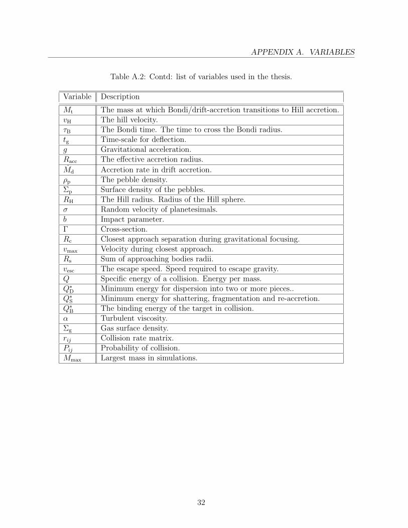
Table A.2: Contd: list of variables used in the thesis.

Variable Description

Mt The mass at which Bondi/drift-accretion transitions to Hill accretion.vH The hill velocity.τB The Bondi time. The time to cross the Bondi radius.tg Time-scale for deflection.g Gravitational acceleration.Racc The effective accretion radius.

Md Accretion rate in drift accretion.ρp The pebble density.Σp Surface density of the pebbles.RH The Hill radius. Radius of the Hill sphere.σ Random velocity of planetesimals.b Impact parameter.Γ Cross-section.Rc Closest approach separation during gravitational focusing.vmax Velocity during closest approach.Rs Sum of approaching bodies radii.vesc The escape speed. Speed required to escape gravity.Q Specific energy of a collision. Energy per mass.Q∗D Minimum energy for dispersion into two or more pieces..Q∗S Minimum energy for shattering, fragmentation and re-accretion.Q∗B The binding energy of the target in collision.α Turbulent viscosity.Σg Gas surface density.rij Collision rate matrix.Pij Probability of collision.Mmax Largest mass in simulations.

32