ACCUMCY OF THE METHOD OF STEEPEST

DESCEKTS FOR A SPHERICAL WAVX PEISETRATING

A PLANAR BOUNDARY

BY James Kurnar Hall

SUBMITTED IN PARTIAL FULFILLMENT OF THE

REQUIREMENTS FOR THE DEGREE OF

MASTER OF SCIENCE

AT

DALHOUSIE UNIVERSITY HALIFAX, NOVA SCOTIA

APRIL 2000

@ Copyright by James Kumar Hall, 2000

National Library 1+1 ,.anada Bibliothèque nationaie du Canada

Acquisitions and Acquisitions et Bibliographie Services services bibliographiques

395 Weiiington Street 395. rue Wellington Ottawa ON K1A O N 4 Ottawa ON K1 A O N 4 Canada Canada

The author has granted a non- L'auteur a accordé une licence non exclusive licence allowing the exclusive permettant à la National Lhrary of Canada to Bibliothèque nationale du Canada de reproduce, loan, distnbute or sell reproduire, prêter, distribuer ou copies of this thesis in microform, vendre des copies de cette thèse sous paper or electronic formats. la forme de microfiche/nlm, de

reproduction sur papier ou sur format électronique.

The author retains ownership of the L'auteur conserve la propriété du copyright in this thesis. Neither the droit d'auteur qui protège cette thèse. thesis nor substantid extracts fiom it Ni la thèse ni des extraits substantiels may be printed or otherwise de celle-ci ne doivent être imprimés reproduced without the author's ou autrement reproduits sans son permission. autorisation-

Contents

Abstract v

Acknowledgements vi

1 Introduction 1

1.1 Theoretical Mode1 of Acoustic Backscatter . . . . . . . . . . . . . . . 2

. . . . . . . . . . . . . 1.2 The Wave Equation in Inhomogeneous Media 2

1.3 Backscatter of a Water-Borne Plane Wave in au Inhomogeneous Sediment 3

2 Reflection and Refraction of Spherical Waves 9

2.1 Decomposition of a Spherical Wave into Plane Waves . . . . . . . . . 9

. . . . . . . . . . . . . . . . 2.2 IntegrdOverthePlaneWaveSpectmm 12

3 The Method of Steepest Descents 14

. . . . . . . . . . . . . . . . . . . . . . . . . . . . 3.1 Coniplex Variables 14

3.1.1 Fhctions of a Complex Variable . . . . . . . . . . . . . . . . 14

. . . . . . . . . . . . . . . . . . . . . . 3.1.2 Mdtivalued h c t i o n s 15

. . . . . . . . . . . . . . . . . . . . . . . . . 3.1.3 Contour Integrals 16

3.1.4 SingdarPointsandBranchPoints . . . . . . . . . . . . . . . 17

. . . . . . . . . . . . . . . . . . . . 3-2 The Method of Steepest Descents 18

4 The Transmitted Wave 34

4.1 TheStationaryPoints . . . . . . . . . . . . . . . . . . . . . . . . . . 34

. . . . . . . . . . . . . . . . . . . . . 4.2 The Steepest Descents Contour 35 . . . . . . . . . . . . . . . . . . . . . . . . . . . . 4.2.1 Branch Cuts 35

. . . . . . . . . . . . . . . . . . . . 4.2.2 Steepest Descents Contour 37 . . . . . . . . . . . . . . . 4.3 Solution of the Tkansmitted Pressure Wave 39

5 Computational Methods 48

. . . . . . . . . . . . . . . . . . . . . . 5.1 Branch Cuts and Sinod arities 48

. . . . . . . . . . . . . . . . . . . . . . . . . . . . . . . . . . 5.2 Contours 53

. . . . . . . . . . . . . . . . . . . . . . . . . 5.3 Computational Methods 55

. . . . . . . . . . . . . . . . . . . . . . . . . . . 5.3.1 MSD contour 56

. . . . . . . . 5.3 -2 "Brekhovskikh's" and Exact Pressure Contours 59

6 Behaviour Near the Critical Angle

7 E'uture Work

Bibliography

Abstract

\men an acoustic wave intercepts the water-seabed boundaq some of the energy

penetrates into the bottom whrle some is subsequently scattered back through the

boundary into the water column. The scattered energy often acts as the background

against which the signal of interest can be measured- A mathematical model for the

scattered energy is discussed for the case of an incident plane wave and scattered

spherical wave- As there is a planar b o u n d q separating the water and seabed, it is

expedient t o perform a plane wave decomposition on the scattered spherical wave. A

steepest descents integration is then used to obtain an approximate solution in the

form of plane waves scattered from each point.

One problem aisociated with the model is that the method of steepest descents

(MSD) fails if the exponential factor in the integrand varies too slowly with respect

to the non-exponential term. This occurs in the vicinity of the critical angle. The

curent research project quantifies the rate of deterioration of the approximation

near the critical angle relative to a more accurate solution obtained by numerical

integration. Some alternative methods to the MSD are also discussed.

Acknowledgement s

1 would like to thank Dr. Paul Hines for his patience, support and much valued

time throughout this project. Thanks also goes to Dr. Ron Kessel for his advice

on numerical contour evaluation and the MSD approach in general. Further thanks

are due to Dr. John Clements for enlightening me on the more theoretical aspects

of complex analysis, and always being kind and encouraging throughout my student

career. 1 would dso Like to thank my parents for their continuous love and support.

Lastly, 1 would like to gratefully acknowledge Defence Research Establishment At-

lantic, Department of National Defence, Goverment of Canada, for permitting me to

complete this thesis while working for them; and Dalhousie University for providing

financial support during course work.

vii

Chapter 1

Introduction

Extensive research has been done in the field of bottom backscatter. Numerous

models have been developed attempting to estimate the maoguitude of backscatter

from the seabed, as well as its dependence upon frequency. grazing angle, bottom

type and roughness.

Hines[5,6] derived one such model. In the model, a plane wave incident from water

penetrat es the planar wat er/sediment interface. Fluctuations in density and acoustic

wave speed nithin the sediment serve to scatter the spherical waves. A plane wave

decomposition is introduced to account for the transmission of the scattered waves

into the water column. The consequent pressure field approximation consists of two

components: a refiact ed plane wave and an evanescent (lateral) wave [G] .

The model was found to be effective in all cases except for grazing angles near criti-

cal, the grazing angle being that between the horizontal and wave vector. One possible

source of the error was the MSD approximation used to detennine the transmitted

pressure fiom the refracted and lateral waves. Near critical the contour integral, from

which the approximation is derived, is known to oscillate rapidly violating the un-

derlying assumptions of the MSD approadi. The approach may fail for such ranges.

Numerical approximations of the integral were compared to the MSD to quant* the

decay. The appropriate contours were chosen and evaluated for different source and

receiver positions at two frequencies. The contours resulting from the MSD approach

were also examined- The effectiveness of the MSD for source and receiver in close

proximity to the interface, which is the niost difficult to model, was then determined.

1.1 Theoretical Mode1 of Acoustic Backscatter

The following outlines the derivation of Hines7s[6] theoretical model for acoustical

backscatter from the sediment volume below a water/bottom interface. The deriva-

tion is developed from the propagation of a plane wave in an inhomogeneous medium.

Since the source is located in the water, the effects of the b o u n d q , which is assumed

smooth, on the transmission must be considered. A function is introduced to d o w

correlation between the individual "scatt ering cent ers" [6].

1.2 The Wave Equation in Inhomogeneous Media

First consider the wave equation in inhomogeneous media. The equation can be

where c is the acoustic wave speed, p the medium density, and p the pressure. Since c

and p are fimctions of position, the medium is inhomogeneous[6]. No general solution

exists for Eq. (1.1). However, if c and p deviate only slightly kom their mean values,

the method of small perturbations can be used to calculate approximate solutions.

First, the fluctuating parameters are expressed as Taylor expansions; retaining only

the first order terms one obtains:

For small perturbations in c and p, the scattered wave will be much smaller in mag-

nitude than the incident wave. Consequently, any reduction in the magnitude of the

incident wave due to scattering is neglected when considering Eq. (1-1).

Expressing the total pressure as the suni of the incident pressure wave pi and the

scattered presswe wave p, yields

Eq. (1.2) is a first-order approximation to the scattered pressure p, in terms of

the incident pressure pi. An approximate solution to Eq. (1.2) for the special case

of backscatter will be considered next. Backscatter occurs when the incident and

scattered wave vectors are anti-paallel, where the incident wave vector is that normal

to wave fkont. The model to be discussed estimates the total backscatter from all the

point sources at the receiver [ô].

1.3 Backscatter of a Water-Borne Plane Wave in

an Inhomogeneous Sediment

Two conditions are placed upon the scattered pressure solution. First, a plane

wave incident fi0111 water refracts into an inhomogeneous fluid bottom composed

of water-saturated sediment. Second, the inhomogeneties behave as point sources

scattering the incident plane wave. The model assumes single scattering only- That

is, the scattered waves resulting from each point source are not scattered again as the

waves propagate to the receiver[ô] .

Figure (1.1) displays the geometry of the backscatter problem. A source is located

a t M which produces a plane wave with incident angle &. The plane wave refracts

into the bottom at an angle 8,. A spherical wave emanates from each scattering

point P. Part of the scattered wave front propagates back to the receiver which is

also located at M [6].

The incident wave pi at any point in the sediment may be written as

pi = PoTsw(Br) exp[iks(rT sin 0, + . w ~ / n ~ - sin2-& - z, COS &)leiwt,

wliere Po is the amplitude of the incident plane wave?

is the pressure transmission coefficient for a plane wave incident from the water and

passing into the sediment, m, = p,/p,, n,, = I / h s = kW/&, and li. and Ii, are

the vectors normal to the wave fi-om, known as acoustic wavenumbers, in the water

and sedinient. respectively. r ~ , rs and zw are s h o w in Figure (1.1). Note that zs is

negative. The evanescent properties of the transmitted wave, at angles of incidence

near x/2: are accounted for by the real part of -iz, k, cos 8, [6].

Substituting Eq. (1.3) into Eq. (1.2) while merentiating the right-hand side of

the Iatt er yields

where the source function Q is given by

The solution to (1.4) is given by a Green's function. For a three- dimensional wave

equat ion

G(r, rr) = QT (expik-T /Ir - ~ ' 1 ) ' (1-6)

wliere G(r. r r ) is a Green's function and Ir - r'l is the magnitude of the vector from

the scattering point to the receiver [6].

Eq. (1.6) States that each scatterer acts as a spherical point source with corn-

plex amplitude Q. The variable T represents the transmission of the spherica. wave

through the boundary. The total scattered pressure is given by the sum of all the

contributing point sources within the isonified volume

Since a planar interface separates the water and sediment: it is necessary to r e p

reseiit eacli scattered spherical wave as an integral over plane waves. Using a plane

wave decomposition, Eq. (1.7) simplifies replacing T by T',. Nonetheless. Eq. (1-7)

is simultaneously replaced by a quintuple integral. The decomposition introduces

a contour integral in the complex plane to represent each scatterer. The contour

integral makes an analytical solution of Eq. (1.7) intractable and a numerical one

unwield y.

The method of steepest descents(MSD) can be used to obtain an approximate

solution to the contour integral. The MSD not o d y simplifies Eq. (1.7) by reducing

it to a triple integral, but also reduces the sum of infinite plane waves into two main

contributions. Each scattered spherical wave can be approximated by two plane wave

components: a scattered refracted wave, p,, and a scattered evanescent (laterd) wave,

PL- The evanescent wave ody occurs when the incident angle is post-critical. That

is, 8 > Oc, where Oc is the critical angle. As Uustrated in Figure (1.2), the refracted

wave propagates dong the Snell's path PQM t o the receiver, whereas the laterai wave

propagates along PSM[G].

After obtaining MSD approximations for p, and pl, the approximation

c m be made. A substitution

q e i k r)/14 = p, + P l ,

of Eq. (1.8) into Eq. (1.7) yields

PS = Q(P, + P [ ) ~ K

The total backscatter of intensity of the isonified volume, I,, will be the sum of the

intensities pSip> over a.ll the pairs of scatterers i and j, where * denotes complex

conjugation: or in integral form [6]

Part of the problem with the mode1 was attributed to the MSD. The MSD fails in

the vicinity of the critical angle where the exponential factor in the integrand varies

too slowly relative to the non-exponential factor.

The curent research project quantifies the deterioration of the MSD approxirna-

tion i l e u the critical angle. The approximation is compared to numerical solutions

of the integral as a function of gazing angle. The symbolic coniputation package,

bIathernaticaTL", was used not o d y to determine the approximations, but also to

examine the behavïour of the associated MSD contour as the critical angle was ap-

proached. Some discussion of alternative methods is also presented.

Before we examine the method of steepest descents, the reflection and refraction

of spherical waves will be briefly discussed. The derivation of the spherical wave

decomposit ion will also be present ed.

Figure 1.1: Schematic of backscatter geometry. The spherical waves are depicted by the ciirved wave fronts.

Figure 1.2: Paths for the backscatter refracted and enavescent(latera1) waves in steep- est descents approximation.

Chapter 2

Reflect ion and Refract ion of

Spherical Waves

Ln the theory of propagation of acoustic waves: it is often necessary to consider the

finite distance of the source of the waves. both from the receiver and the boundaries

of the medium. The sirnplest problem of such nature involves a point source located

a finite distance kom a plane interface between two homogeneous media, resulting

in the reflection and refraction of a spherical wave. The basic solution requires the

expansion of spherical waves as plane waves [3].

2.1 Decomposition of a Spherical Wave into Plane

Waves

The ciifference between the symmetnes of the wave and the f o m of the boundary

account for the difEculties with the reflection and refkaction of a sphericd wave on a

plane interface between two media. Although the wave has spherical symmetr); the

boundazy is planar. Hence, the problem is solved by expanclhg the spherical wave in

plane waves [3].

Firsr. the spherical wave is expressed as

where the source is located at the origin, R = (x2 + y2 + z') ' /~ 131-

In the z = O plane, the field of the spherical wave will have the form eik/r, where

r = (x2 + y2)1/2- Using [3] a double Fourier integrai in x and y:

where A(kz. k,J is defined by

and kx' I*, are the component wave vectors.

Let

k, = qcosll>, k, = qsin*, q = (k: + k:)'I2

Then Eq. (2.2) becomes

The iiltega.1 over r is easil- obtained. F'urthermore, assuming that there is some ab-

sorption in the medium, that is, k has a positive imaginary part, then by substitution

of the upper limit over r, letting b = @ - #, and using symmetry, we have

Eq. (2.7) describes the spherical wave in xy-space. Introducing the following tenn

in the exponential under the integral:

9 =tikzz. whew k= E (k- - k: - k y - (2-8)

Brekhovskikh[3] "continues" Eq. (2.7) in space. The plus s i p s correspond to all

points in the half-space z > O where the waves propagate in the direction of positive

z. The converse holds for the minus siga Hence.

Eq. (2.9) represents the expansion of a spherical wave into plane waves. The exponent

under the integral is that of the plane wave. The direction of propagation is given by

the values of the components of the wave vectors kz7 5, kz [3].

The integration in Eq. (2.9) over the horizontal components k* and k, of the wave

vector k c m be replaced by integration using the angles B and @. The latter represent

the direction of propagation of each of the plane waves. Letting

the integration is performed over 4 between zero and 2w. R e c a h g Eq. ( M ) , kz

changes komIÎ, = k for k, = li, = O to li, 4 oo for k, 4 fca or + &ca [3].

From Eq. (2.101, cos9 = k z / k . Thus, 0 will var). frorn B = O to 8 = n / 2 - icm.

Applying the formulas for the transformation of variables yields

dlc,dkydlî, = Ic, sin BdBdO.

Consequently, Eq. (2.9) c m be rewritten as

eikR x/2-i00 2ïr i" / ei(k.=+kyg+k=z) z)O, -=- sin Bd+de R 2x O

2.2 Integral Over the Plane Wave Spectrum

Recall Figure (1.2) wliich illustrates the geometry of the situation. The interface

Les along the Iine r = O. The receiver, M, is located on the r axis at a heiglit

- The source P' located at depth 2,: produces a spherical wave. The angles 6'

and + represent the complex angles of incidence and refraction in the plane wave

decomposition. The angle ;3 will be discussed later[5].

Representing the integral over a plane wave expression (recall Eq. (2.11)), gives

The phase term corresponds to the segment P Q M in Figure (1.2)

where zs < O since P is below the interface[5].

To obtain the pressure at hll the effect of the interface must be incorporated. This

is achieved by multiplying each

Tsw (8)

plane wave component by the transmission

- 2ms, cos O - m, cos O + 4-'

Thus, the transmitted pressure, pt , becomes

eiks (TT sin 13-zs cos 8+r, J-)

The integral over d$ c m be easily solved [Il to obtain:

icc

pt = i k , JI-- Jo(u)eiks(~J-e-zS c o . s ~ ) ~ .,(O) sin Ode.

where u = k , r ~ sin 6- Rewriting the Bessel function as a sum of Hankel

yields

coefficient

(2.15)

funct ions

Lastly retaining only the first term of the aqmptotic expansion

'1 (,) (2/?ru) 112 eXpi(~-x/2) (1 + l / â 2 ~ + - - -)

one obtains

An approximate solution to Eq. (2.17) can be obtained by ushg the method of s t e e g

est descents(MSD)[5]. However, before discussing the solution, the MSD and some of

the basic concepts of complex analysis from which it is derived WU be presented.

Chapter 3

The Method of Steepest Descents

3.1 Complex Variables

Before discussing the Method of Steepest Descents(MSD) , some basic concepts

from complex analysis central t o the problem will be reviewed.

3.1.1 Functions of a Complex Variable

First recall that a complex number is nothing more than an ordered pair of num-

bers. Similarly, a cornplex variable is an ordered pair of two real variabies[2],

z = (x, y) = x + i y .

A graphical representation is usually employed to display a complex variable. x?

the real part of z: is plotted on the abscissa and y, the irnaginan; part of z , ou the

ordinate. This results in the complex or Argand plane[2].

From this plane the following simple geometrical arguments are obtained

Thus,

or using a polar representation[t]

To ex-tend complex variables to the realm of functions, the convention of represent-

h g the functions as the ordered pair (u(x, y), v(x, y)) is adopted. Cornplex functions

can be resolved into real and imaginaq parts

where u(x, y) and v ( x , y) are pure rea1[2].

The real part of a fùnction w(z) is oken Iabelled as IR f ( z ) whereas the ima,@nary

part is labelled S f (z). Thus, in Eq. (3.1)

Ef (z) = u(x7 y), and %f (2) = v(x, Y)-

The Cauchy-Riemann equations

must hold for the derivative of a complex function to exïst [2].

From these conditions the followïng defkitions result. If f (2) is differentiable at

z = zo and in some small region around zo, then f (2) is analytic at z = ZO. If f (ro) is

analytic eveqwhere in the (finite) compIex plane, then it is c d e d an entire function.

On the other hand, if f (r) does not exid at z = 20, then 10 is labeled a singular point

Pl -

3.1.2 Mult ivalued Functions

All elementary functions of real may be extended into the complex plane.

The real variable x need only be replaced by the complex variable 2. Nevertheless,

there are occasional complications. For example, the logarithm of a complex variable

may be expanded using the polar representation

= l n r + ie.

This representation is incomplete. Any integral multiple of 27ï can be added to the

phase angle 8. The value of z will not change. Hence, Eq. (3.2) [2] should actually be

The funct io~ in z is termed a multivalued fimction. It has an infinite number of

values for a single pair of real values r and 8. By convention n is set to zero to avoid

any ambiguity and the phase limited to any interval extending over 27r radians. The

line in the z-plane that is not crossed, which in this case is the negative real axis, is

knows as a cut line or in some texts as a branch lzne or branch cut. The value of ln z

with n = O is called the principal value of Ln z [2]. The concept of branch lines will

be considered in more detail later.

3.1.3 Contour Integrals

Using the analogy of an integral of a real function integrated along the real x-axïs,

the integral of a complex variable over a contour in the complex plane may be defined.

Let the contour zozo be divided into n intelvals by picking n - 1 points along the

contour. Consider the s u .

where C, is a point on the curve between tj and rj-1. Let n -+ oo with

for al1 j. If lim,,, Sn exists, then

The right-hand side of Eq. (3.4) is the contour integral of f (z) dong the contour C

from z = zo to r = zk. For an analytic function the line integral is a function only of

its end points, independent of the path of integration(21:

3.1.4 Singular Points and Branch Points

A few more definitions are necessq before the method of steepest descents can

be considered. Fi& the point ro is an isolated singular point of f (z), if f ( z ) is not

analytic at r = 20, but is analytic at au neighbouring points[2].

We consider a type of singularity known as a branch point. Let

where a is not an integer. As z moves around the unit circle kom eo to e2x', f (z)

approaches e2"ai # eo, for nonintegrai a. eo and e'"' coincide in the z-plane, but these

two points lead to dif ferent values of f (2). This point is known as a branch point and

f is a multivalued function [2].

For example, let a = 1/2. Then r = reie such that f (z) = fieie'*. Let f ( z )

make a complete circuit(counterc1ockwise) around the origin starting at 0 = where

f (2) = J;eiel/2- At 8 = Oi + 27r, f ( z ) = -fie'el/2, whereas at 6 = Oi + 47r, f ( r ) = fieie2/2 again [8].

This situation can be described by saying for O 5 6 < 27r we are on one branch of

the function, whereas for 2n 5 0 < 47r we are on a difTerent branch [8].

Each branch of the function is single-valued. Creating a cut line from the origin

to infinity on the real axis allows the function to always be single valued[8].

A cut line will allow f ( z ) to be uniquely specified for any given point. However,

a function with a branch point and a cut line will not be continuous across the cut

line. There will be a phase difference on opposite sides of the cut line. Hence, the

integrals on opposite sides of the branch line will not cancel out [2].

Fomally, a point z = zo is c d e d a brunch point of the multivalued function f (2)

if the branches of f (z) are interchanged when z describes a closed path around 20.

There is a n alternative method for achieving the cut line described above. Imagine

that the z plane consists of two sheets superimposed upon each other. The sheets

are cut dong the cut line. The lower edge of the bottom sheet is joined to the upper

edge of the top sheet. Starting in the bottom sheet and making one complete circuit

about the origin one arrives at the top sheet. Imagining that the other cut edges are

joined together? if the circuit is continued the top sheet can be returned to from the

bottom sheet [8].

The collection of two sheets is hown as a Riemann surface, In this case the

surface corresponds to the function z ' / ~ . Each sheet corresponds to a branch of the

function. On each sheet the hinction is single-valued[8].

The Riemarin surface allows the values of the mdtivalued function to be obtained

in a continuous function- Futhermore, the concept is easily extended to other func-

tions. For esample, 2'13 has a Riemann surface composed of three sheets. 1Vherea.s

ln z would have a surface composed of infinitely many sheet s [8].

Fiames (3.1) through to (3.4) display some examples of branch cuts. Figure

(3.5) shows how the two Riemann sheets when superimposed produce two contînuous

surfaces. Fiogre (3.6) displays the same two sheets joined dong the branch cut.

These cuts occur in the integrand from the transmitted pressure integral and d l be

discussed again later.

Using these toois from cornplex analysis, the method of steepest descents can now

be examined.

3.2 The Method of Steepest Descents

In problemç from mathematical physics it is often necessq to determine the

behaviour of a h c t i o n for large values of the variable[2]. If the function can be

then the method of steepest descents can be used to determine its asymptotic be-

haviour in S.

Take s to be large and real and both f (2) and F(r ) analytic. The contour C

must then be chosen such that the real part of f (2) approaches minus infinity at both

limits and the integrand vanishes. Alternatively it can be a closed contour[2, 31.

If s is positive and large. then the value of the integral d . l also become large when

the real part of f (2) is large. On the other handl when the real part of f (r) is s m d

or negative. the value of the integral Ml1 also be srnall. If s increaçes indefinitely, the

entire contribution of the integral dl corne from the region in wliicli the real part of

f (2) has a positive maximum value. Away from this region the integral will become

increasingly small provided F (t) is slowly varying [2, 31.

Under these conditions, a cornparatively short path of integration can be chosen.

This path \vil1 effectiveIy determine the entire value of the integral. Tlien the inte-

grand can be replaced by a simpler function tichich is identical to the integral dong

this path. The behaviour of the integral dong the remaining p m s of the path can

be ignored[3].

Expressing f (2) as

f (z) = u(x, y) + iv(x? y) Eq. (3.6) can be rewritten[2] as

Non., in addition. are impose the condition that the ima,@.nary pazt of the exponent,

iv(xl y). is constant in the region where the red part takes on its maximum value,

that is,

The integral inay then be approximated by

I ( s ) = eiSv0 F (~)e'"('~~)dr.

Away from the maximum of the real part, the imaginazy part may oscillate. In these

areas the int egrand is negligibly small and the varyïng phase factor is inconsequent ial[2].

The real part of s f (2) is a maximum for a given s when the real part of f (z),

u(x, y), is a maximum. This implies that

Recalling the Cauchy-Riemann conditions[2], it follows then that

Some observations must be made before the roots of Eq. (3.7) are obtained. First.

the mituinium value of u(r. y ) is the maximum only along a certain contour. In the

f i t e plane neither the real nor the imaginary part of the analytic function have

an absolute rnayuimum. This becornes clear when recalling that both the real and

Maginary parts of an analytic function must sati* Laplace's equation[8]

Frorn Laplace's equation it follows that if the second derivative wïth respect to x is

positive, then the second derivative with respect to y must be negative, or vice-versa.

Hence, neither u nor v can possess an absolute maximum or minimum. Since f ( 2 ) is

analytic, sin,dar points are excluded. The vanishing of the derivative then implies

that w-e have a saddle point, or a stationary valueo TV-hich ma? be a maximum of u ( x , y)

for one contour and a minimum for another [2].

The most convenient path of integration should thus pass through the saddle point

detennined from Eq. (3-7) and away fÎom it along the line v(x, y ) = constant. Such a

path is ofken referred to as the saddle point path of integration or the path of steepest

descent. If s is luge: then the exponent

Nill fall off rapidly as the contour departs from the saddle point. Hence, only a small

part of the path which includes the saddle point will contribute s i ,~can t ly to the

int egrat ion [3].

Thus, it is necessaq to chose a contour of integration that satisfies two conditions:

0 u(x, y) has a maximum at the saddle point.

r The contour must pass through the saddle in such a way that the imaginary

part, v(x, y), is constant[2]-

Great care must be taken to ensure tliat the line of steepest descent is distinguished

from that of steepest ascent. The line of steepest ascent is also characterized by a

constant v. The saddle point must be carefully inspected to distinguish these two[2].

Fi,gures (3.7) and (3.8) show an example of a saddle point and Line of constant

phase respectively. The dotted line indicates the steepest descents contour. The dot

in the centre of the contour is the stationary point- The chosen function is that fiom

the transmitted pressure Eq. (2.17).

At the saddle point the function f (2) can be expanded in a Taylor series to give

From Eq. (3.7), the first derivative need not be considered. The second term in the

expansion is real and negative. It is real because the imaginary part must be constant

dong the chosen contour. It is negative because the contour will be traversed down

from the saddle point. Hence, assuming f "(zo) # O, it follows that

which serves t O define a new variable t [Z] .

If ( z - zO) is written in polar form

where a is held constant, then

The phase of the contour at the saddle point, which is specified by a, is chosen so

that 3[ f (z) - f (q)] is identically zero. Since $ ( z - z,)* f" (q), t is real, and may be

written as

t = ~ d l s f " ( ~ ~ ) I ~ / ~ . (3.10)

Siibstit~iting Eq. (3.8) into Eq. (3.6): gives

From Eq. (3.9) and Eq. (3.10)

Thus, Eq. (3.11) becomes

It should be noted that the limits have been set as minus infiiiity to plus infinit3r.

This is allowed so that the integrand will be essentially zero as t departs from the

on- [al - Noting that the remaining integral is just a Gauss error integral equal to 6,

the following is obtained:

The phase a, introduced in Eq. (3.9), is the phase of the contour as it passes

through the saddle point. This is chosen such that

a a is a constant; and

Rf (2) is a maximum [2].

If the contour passes through two or more saddle points in succession, then the

contributions from each point should be summed to get an approximation for the

int egral [2].

One ha1 observation is necessary. It was assumed that the only major contri-

bution to the integral came from the vicinity of the saddle point(s) z = 20, that

is

W(4 = u(x, y) ~ ( x o . YO)

over the entire contour away from 20 = x + iyo. This condition nmst be carefully

checked for every problem [2].

Brekhovskikh[3] presents an alternative formulation of the MSD than the preced-

ing obtained fton Artken[2]. Brekhovskikh's does not consider the phase, a, of the

contour as it passes t hrough the stationary point.

First performing the change of variable from z to o in Eq. (3.6),

is defined. The saddle path Nill consist of the locus of points determined by the

equation

f (2) = f (ro) - 2. (3.15)

where a is real, -00 < a < cm. The saddle point is given by a = 0- Taking the real

and imaginary parts of Eq. (3.15) yields

s f ( r ) = §f (to), and Rf (2) = Rf(zo) - 0'

As required, the imaginary part of f (2) remains constant: while the real part, which

is maximal at

w - From Eq.

saddle cari be

o = 0, decays as the contour departs from the saddle in nny direction

(3.14) and Eq. (3.15), the original integral Eq. (3.6) taken dong the

rewritten as

As s is assumed large, only s m d values of a are consequential in the integrand.

Hence, @(a) can be represented as a power series in o as:

Substitut ing this series into the integral and observing t hat

: it follows that

This derivation permits a representation of the values of the integral in the form of a

series of inverse powers of the large parameter S . If <P (o) varies slowly in cornparison

*th the exponential te-, e-Ss, that is if its derivatives are sutficiently s m d ' then

the approximation (3.16) can be limited to the first or first fen- terms [3].

Considering only the terms in Eq. (3.16): first differentiate Eq. (3.15) with respect

to O_ f f ( z )dz /da = -20. Substituting dz/do into Eq. (3.14) yields

Representing the functions f ( z ) and F ( t ) in the form of series of powers of x = z - =O:

f (z) = f (zo) - A X ~ + 13x3 + CX' + - - -

F ( z ) = F(rO)[l + PX + Q X ~ + - . -1, P - Ff ( to ) /F ( zo ) , Q F"(zo)/2F(zo).

From Eq. (3.18), Eq. (3.15) yields

Inverting the series, x can be represented in the form of a series of powers of o:

Equating coefficients of like powers of O:

From Eq. (3.17): Eq. (3.18) and Eq. (3.19)?

Substituting the value of x fiom (3-21), @(O) c m be represented in the form of a

power series in O:

Considering Eq. (3.21): near the saddle point, x = t - zo = o / a . Therefore, if

O > O, then a r g ( l / J A ) = arg(z - zo)- The sign of the square mot is obtained hom

arg (z - to) [3].

From the values of A, B, C, P, and Q, Eq. (19) and Eq- (20) yield

1 f" Ff 1 fIV -@"(O) = @(O) [ 5 --+------- 2

" 1 . ( y y ~ 4(py 12(fq3 ~ f " - These expressions solve (3.16) [3].

Figure 3.1: First Riemann Sheets for R f (0) in the vicinity of the origin.

Figure 3.2: Second Riemann Sheets for R f ( O ) in the vicinity of the origin.

Figure 3.3: First Riemann Sheets for R f (0) in the vicinity of the critical angle&).

Figure 3.4: Second Riemann Sheets for R f (8) in the vicinity of the critical angle&).

Figure 3.5: Superimposed Sheets for R f ( O ) in the vicinity of the critical angle(&).

Figure 3.6: Sheets joined for Of (0) in the vicinity of the critical angle.

Figure 3.7: Saddle Point for R j ( 8 ) kom transmitted pressure integral.

Figure 3.8: Line of Contant Phase for S f (6) ftom transrnitted pressure integral.

Chapter 4

The Transmitted Wave

Recalling the transmitted pressure integral, Eq. (2.17), the MSD approach will

now be considered. The related contour will also be discussed with some atte~ltion

placed on the role of branch cuts resulting fiom the integrand.

4.1 The Stationary Points

To obtain the stationaq points

must be solved. The solutions of Eq. (4.1) have physical meaning if it is rewritten in

terms of $J: the incident angle in the water, as opposed to 8, the incident angle in the

sediment (see Figure (1.1)). This yields

z, sin @cos$ r~ cos @ - z, sin 10 t d-.

One solution of Eq. (4.3) is given by + = $+_ where y, is

= o. (4-3)

the pure real angle

of refraction given by Snell's law(see Figure (1.2)). This can be deinonstrated by

34

observing that

2 sin 0,- = n,, sin g!+ y cos 8, = (1 - n,, sin2 &) I l2 . (4-5)

The angle 10, is most easily found numerically[5].

A second complex solution of Eq. (4.3) can also be found. First observe that the

fîrst two terms of Eq. (4.3) sum to zero when TT cos ?Ir = z, sin Sr, which corresponds

t o the angle 0 in Figure (1.1)

The secondary stationary point has the form

with 4 cornplex and 141 << ,û. A Taylor expansion of f f ( @ l ) = O around B yields

The secondary stationary point corresponds to the angle of transmission of the lateral

wave [5] .

4.2 The Steepest Descents Contour

4.2.1 Branch Cuts

sin .iCI is nml- Before discussing the steepest descents contour, note that

tivdued. This term occurs both in the denominator of T,(@) and in f(@)- Conse-

quently, branch lines will occur in the compIex plane. The standard choice of branch

line for the square root of a complex nuinber is the negative real axis. However,

Brekhovskikh chose the positive real axis. Consequently, his branch lines are given

b_v

l - n & s i n ' d ~ = ~ ~ ; 0 < q ~ c x > (4.10)

or 2 1/2 s i n + = ( l - q ) ln, (4.11)

where q is real. Letting $J = $'+i?,V"' sin $J can be expressed in its real and imaginary

Pa=-

sin @ = sin(#) cash(@"' + i cos(@) siah(qY"'. (4.12)

When q > 1, Eq. (4.10) becomes:

sin @ =

where y is real. This can only hold if @' = O- As q -+ 00, (@'. 11") = (0, *oo)[5].

If q = 1, Eq. (4.10) becomes:

sÙz?.b=O

which requires (+': @"' = (0,O) for the given domain of integration. Findly if q = 0,

Eq. (4.10) becomes

sin $.J = &l/n,

for which (Ur', ?lin) = (d&, O) where $c >c sin-'(lin,). Thus' the branch h e s nin

from [-$c, ?ire] along the real axis and from (-oo, co) along the irnaginary axis[5].

Observing that if

such t hat

the same result can be obtained by solving the pair of equations

These two conditions define where (n:, - sin2($)) lies on the positive real-axis,

Brekhovçkikh's [3] choice of brandi cut-

4.2.2 Steepest Descents Contour

To obtain the steepest

must be solved. By virtue

descents contour

CF( f (@)) = constant

of the i multiplier, this is equivalent to

Following Brekhovskikh%[S] convention, the "upper" Riemann surface is defined by

(1 - nl, sin2 $) > O

and the 'Lloa~er77 by

(1 - ny, sin2 +) < O.

The two sheets are joined together on the lines S(n& - sin2 +)'/* = O. which begin

at the branch points. 1L, = & arcsinnws[3, 51.

As zb" -+ x, Eq. (4.16) becomes

rTR sin @ + z,E cos @ - zsR(* sin @) = constant.

where -i sin tb is the upper Riemann surface and +i sin @ the lower surface. Recding

Eq. (4.12) and noting that

COS $J = COS @' cosh $JI' - i sin +'sinh +"

Eq. (4.16) simplifies to

(rT sin 21>' + zw cos d) cosh $' + z,(& cos 21') sinh #' = castant . (4.18)

As IY~ -+ oc cosh $Ir" and sinh 21'' are both dominated by e$''/2. Thus. Eq. (4.17) will

ody remain finite if the coefficients of cash@" and sinh+If sum to zero resulting in

r~ sin y' + zW COS $' f COS $JI = 0. (4.19)

Solvïng Eq. (4.19) for 1u" = +CO: on the upper surface $' = - tan-'((z, - zs/rT) and

$J' = tan-' ((z,,,+zS)/rT) on the lower surface. Using a similar argument for +" = -a>,

Sr' = T - tan-' ((zw - ZJ/TT) on the upper surface and @' = .rr - tan-' ((% + zs) /rT) on

the lower surface. iï enters the expression because the contour approaches $" = -cm

in the quadrant 7~/2 5 zb' 5 ~ [ 5 ] .

Using the above limits. the contour for Eq. (4.16) can be plotted. When ,û < 10c the contour begins on the upper Riemann surface at ($', Q") = (- tan-'((, - ) / r ) , ) At $' = O it crosses the branch h e and enters the lower Riemann

surface. At the Stationary point it crosses back ont0 the upper Riemann surface

and continues to (1L', +") = (n - tan-'((2, - z , ) / s ) , -CO). Hence, for 0 < 11, the

second stationary point does not enter the result[5]. Figure (4.1) shows the passage

path originally used by Brekhovskikh[3] and the deformed MSD passage path. The

dotted lines in Fi,wes (4.2) and (4.3) illustrate an example of the deformed contour.

Figure (4.2) is the real part of f (S>) corresponding to the path of steepest descents

and (4.3) is the imaginary part corresponding to the line of constant phase. Since the

contour only changes surfaces twice when P < @, it is not difficult to plot f (+). The

first and third quadrants of the complex plane are the fist surface whereas the second

and fourth are the second- As required, Figure (4.2) displays a saddle, whereas (4.3)

displays the constant phase along the MSD path.

Fig-ure (4.4) displays the different surfaces that the contour crosses. The solid

lines indicate the &st Riemann sheet and the dotted line the second.

If @ > &, the contour is much more complicated. Referring to Figure ( 4 4 ,

starting a t ( , ) = (- tan-'((& - z,)/s), m), the contour proceeds along the

upper surface to the imaginary axis where it continues ont0 the lower surface. The

contour continues to the branch line at $Ir = O, where it passes through .Sr, and then

crosses back onto the upper surface. However, provided

the contour now recrosses the S>' axis at 11. and heads back to the $" axis. If

the latter condition does not hold, the contour behaves exactly as it does when

< continuhg to ($+? d~") = (a - tan-'((-, - zs) /rT) : -00). Crossing the imag-

i s q - axis, the contour remains on the lower surface where it approaches (@', +") =

(- tan-l((av i ts)/rr). m). The contour must begin and end on the same Rie-

mann surface. Thus, a second segment of the contour is added. Beginning at

(+': @") = (- tan-'((, tz,) IrT), ca) on the lower surface, it procedes along the Ionver

surface to the z!~" axis, where it crosses onto the upper surface and passes through

the second stationary point, wl- The contour remains on the upper surface, crossing

the real axis t o the right of the branch point at ~ c . The contour then approaches

($':$") = (T - tan-'((r, - 4)/~=): -03). Hence; for ,û > lLc, the contribution fiom

both the rekactive and lateral stationary points much be included[5]. Figure (4.5)

shows the passage path if ,û > $JC. Figure (4.6) illustrates an example of such a

contour. The thiclmess of the line is proportionai to the magnitude of f ( O ) . Figure

(4.7) dîsplays an enlargement of the region around the Snell and lateral angles for the

same contour-

4.3 Solution of the Transmitted Pressure Wave

Following the procedure discussed above, it remains only t o employ the formulae

given in Chapter (3) and obtain a solution for p, = p, + pl. For Eq. (2.17)

f (6) = i(rT sin 0 + , Jn&, - sin2 û - zS COS O )

F ( O ) = T,, (0) m. (4.20)

Consequently Brekhovskikh's [3] RiISD approximation using only one t erm becomes

ilî,(rTsinO, + zwJ-- z, cos~ , )

where 0, is the angle of rekaction of the wave below the interface, that is sin 8, =

n,, sin dT [5]. &&en's approximation' [2] , O&- m e r s slightly, the most important

addition being the eiP multiplier; where a is the phase of the contour at the saddle

point [2 j .

MSD contour

branch line

Figure 4.1: Passage path and Brekhovskikh's ori,@.nal contour for f ($) when < Sc

Fiorne 4.2: Contour plot of real part of f ($) where 4 < &

Figure 4.3: Contour plot of imaginary part of f (i>) where ,û < $c

Figure 4-4: change of Riemann sheets where 0 <

Brekhovskikh contour

branch fine

-1 713 - tan

Figure 4.5: Passage path and Brekhovskikh's original contour for f (e) when ,O > zbc

Figure 4.6: Magnitude of f (S) when ,B > Src. Thickness of h e indicates magnitude of int egrand.

Figure 4.7: Contour in vicinity of snell and lateral angles for /3 > ?,bC.

Chapter 5

Comput at ional Met hods

The numerical integration and MSD approximation of the pressure integral were

performed by the symbolic computation package MathematicaTA'. However, consid-

erable analysis of the integrand was performed by the author prior to obtaining either

estimate. The branch cuts and singularities occuring in the integrand were exaniined

first .

5.1 Branch Cuts and Singularities

First. the branch cuts in the integrand were considered. hlathernatica'sTM [9]

default choice of branch cut for the square root function lies on the negative real axis.

This is the common alternative choice to that made by Brelihovskikh[S]. For this

choice, the branch cuts of the composite function

lie on the lines at f 7r/2, (-00, -Src] and [QC, oc) where

The latter is demonstrated

R(ny, - sin2(@)) < O

%(nL - sin2($)) = O.

in Appendix (A).

Both choices of branch cuts were considered in the hfathematicaT"' implenienta-

tion. Initiallg., the default choice of the negative real-axis was used. Later the author

as able to ernploy Brekhovskikh's[3] branch cuts by replacing Mat hernatica'sT"'

built-in square root function 6 t h his o m . The choice of negative real axis as a

branch results fiom klathematica'sTM argument function, Arg[z]. The function re-

turns values in the range [-T, n]' providing a branch line along the negative real-axis

to maintain

The tti-O

princi ple-valuedness [9] - square roots of a complex number[8] are given by

Replaculg r1I2 with J ~ b s [ z ] and 0 with Arg[z] two fûnctions can be defined for the

two roots. For k = 1, it can be clemonstrated (by expanding cos and sin) that the

two roots are negatives of one another. Thus? the first function returns the square

root where k = O. The second returns the negative of the hrst.

In general, the principle argument of z = x + iy[7] is given by

This definition creates a branch cut along the negative real-axis. A similar definition

is used in ~vlathematica's~" ïmplementation of arg for z # O- Writing a function that

defiaes arg as

arccos(x/ 1.1) if y 2 O! arg z =

x-arccos(x/lzl) if y < O

produces values in the range [O, K] creating the cut dong the positive real-axis. The

same cut Fvill appear when calculating the square roots.

It is important to note that, regardess of the choice of cut, no assignment of arg t

is made to the complex number zero[?]. This issue will be considered again later when

evaming the contours available for solving Eq. (2.17).

Regardless of the choice of branch cut, the same contours are obtained. Difficdties,

however. arise nith Mathematica'sT" choice. When ,û < q!~, in the vicinity of the

refractive stationary point, only the branch a t i r /2 is crossed. Hence, it is unclear

when the contour w d l cross a second cut and return to the surface where it began.

Using Brekhovskikh's[S] cuts the contour clearly be-ins and ends on the same surface.

Nonetheless. the solutions for both sets of cuts remain the same. The conclusion can

be drawn that the contribution to the integrand outside the immediate vicinity of the

stationary points is negligible. The latter being one of the justifications for the MSD

approximation.

Brekhovskikh's choice of cuts also simplifies the procedures used to obtain each

contour- hlathernatica'sT'L1 FindRoot function c m be used to solve

3( f (Q)) - constant = O

where the constant equals S f (&). The cuts allow- the (@', +") plane to be divided

into four regions where the appropriate se-gments of each contour can be found. This

issue will be discussed at length in the following section.

The behaviour of the non-exponential term of the integrand was also examined.

The non-exponential factor

introduces a second branch cut in the complex plane, as well as a series of poles.

From sin(^), depending upon the choice of the branch lines, an additional cut

is necessq on either the negative or positive real-&S. Setting li, = @' + i$" and

expanding sin in terms of its real and imaginary parts gives

and

%(sin p5) = COS(?^) snh(7ft) - (5.2)

First, Eq. (5.1) and Eq. (5.2) are both zero a t the origin, the branch point. The

branch cut will lie on the negative real-axis when Eq. (5.1) is negative and Eq. (5.2)

is identically zero. Eq. (5.2) is identically zero if t!~' = frir/3 and/or @" = O. To

obtain the cuts? the following three cases are considered.

First. if @' = =tir/2 and .SI" # O, then Rsin @ = coçh(tb") for +' = n / 2 and

- cosh(z9") othemise. Since, = cash(@") 5 -1, Eq. (5.1) is negative only when

d~' = -n/3 for al1 y'' except zero.

Secondly, if 1u' .f +z/2 and tb" = O, then

'8 sin (zb) = sin(+').

sin(?i.') < O when - ~ / 2 < < 0.

Lad'-, if +' = &n/2 and d~" = O? then

?lif must be -z/2 for R sin@) < 0.

From the three above requirernents, the branch cut is dehed m-hen

{er = -7ï/2, all 20") and { -~ i /2 < @' < O and +" = O}.

Alternatively, if the branch line for the square root is chosen to be on the positive

real-aïs. the branch cut will instead lie on

(20' = ~ / 7 , al1 +") and {O < @' < ir/2 and d' = 0)

using the same arguments as above.

Recall that 2m,, cos @

T,,(+) = m,, cos iii + J-'

The terrn Jnz, - sin2 $J has already been considered at length for f (v). Hence, the

ody other sinOgularities occur when the denominator of T,,(S>) is zero: or

These singularities are poles. The denominator is zero[3] when

2 Since ntsw > nWS and m, > 1: (m.:, - n:s)/(m:m - 1) > O. expansion of sin+:

sin = sin tb' cosh @" + i cos tb' sinh t5"

sin $' cosh Wu = =t,

COS yl' sinh +" = 0.

sinh +'' = O only when $" = O. If d~" = O, then Eq. (5.4) becomes

(5-3)

Using the coniples

2 sin w' = f m:w - %s

m:, - 1 .

For 1 sin @'l 5 1. This requires

which is not possible[3].

Hence, +' = f î ~ / 2 for Eq. (5.5) to hold. If zb' = s/2, Eq. (5.4) becomes

cash$" 2 1 so only the positive case need be considered. Since

holds, Eq. (5.6) Rill have the two solutions

as 7-22, # 1[3].

If @' = -7r/2, the same solution is obtained. Kence, there are four poles:

3. $J' = n/2, +If < O; and

Poles 1 and 2 are symmetric with respect to the origin, as are 3 and 4. By determining

the sign of Q(nL - sin2 y)'/* and using Eq. (5.3)? it can be easily demonstrated

that poles 1 and 2 lie on the upper, and 3 and 4 on the lower sheet when using

Brekhovsklkh7s choice of cuts[3]. Provided the chosen contour does not pass through

any of the above poles, their contribution t O the integrand is inconsequential.

5.2 Contours

Several contours were considered by the author mhen evaluating the integrd nu-

merically. The first is illustrated in Figure (5.1). The segments near the real axis

were chosen such that the contour would never pass through the origin and critical

angle, where the square root ternis in the integrand are undefined. Furthermore, if

the contour starts on the upper surface at icx, - x / 2 and ends on the same surface at

7r/2 - im, then the two segments along f r / 2 do not cross any poles, since poles 3

and 4 lie on the lower sheet and 1 and 2 are not on the contour.

The second contour chosen was that resulting frorn the MSD approximation. As

discussed in Chapter (4), two contours are possible based upon which of 0 and &

is greater. Neither contour crosses any poles. Nevertheless. some care is required

when considering the cuts kom the non-exponential term ,/sin($)- When 0 < WC, the MSD contour nrill cross fiom the upper to lower surface at ~ / 2 . Consequentially,

the contour will end on t h e lower surface a t 7r/2 - zoo instead of the upper surface.

The contour Rill similady end on the wong surface when ,û > Vc. The additional

branches require a change in sheets not onIy at lr/2: but also after the contour has

passed through the snell's law angle and recrossed the real axis between -& and 0. Brekhovskikh[3] does mot consider the cutç fkom Jw. However, a physical

condition is provided which justifies the use of the branches from the J- te- alone. The sign ascribed to J-. must be such that the imaginary

part of f (u) is always positive. Otherwise, the wave will appear to be exponentially

increasing wïth depth. O n physical grounds, this is unacceptable [3].

When 0 > +c, if the Lower sheet is used for the segment of the contour passing

through the laterd stationary point, Brekhovskikh's condition is not satisfied. Fur-

thermore, when B < $ J ~ , if the lower sheet is used after 7~/2 is crossed, the integrand

grows exponentially as the contour approaches 7r/2 - im. Use of the cuts from the

transmission coefficient a n d f ($) further justiS the assumption that the integrand

is dominated by the exponential term. This assumption is necessary when using the

hfSD approximation.

The third contour chosen was that from Eq. (2.15). This integral represents the

exact pressure. The Bessel function has not been replaced by the Hankel function

which is subsequently asymptoticdy expanded. Unfort unately, the MSD cannot be

applied to this equation. Appendix (B) discusses the properties of the integrand

which prevent this approach being possible. The contour was chosen to nin along

[O, ~ / 2 ] and then ftom i r /2 to 7r/2 - ix. The need to only integrate to 7r/2 - i~ will be discussed in the next section. For this integral, passing through the critical

angle was not found to be problematic. Fùrthermore, the square root term in the

non-exponential factor is not present. So the issue does not arise when evaluating the

latter.

The contour associated ccfith the MSD approximation wiil be referred to as the

"MSD contour". whereas that composed of five simple linear segments will be re-

ferred t O as "Brekhovskilih's" contour. "Brekhovskikh's" as the contour considered

in Brekhovskikh[3] prior t o his discussion of the MSD approach largely resembles

that discussed above. starting at - ~ / 2 + iw_ proceeding to the real axis at - ~ / 2 ,

continuhg tu ~ / 2 , then approaching the lower endpoint at ?r/2 - iw. The contour

for equation (2.15) wiIl be referred to as "exact".

5.3 Computational Methods

Only one of the above contours was used for cornparison with MSD. Numerical

evaluation of the exact pressure, Eq. (2.15), was found to be the easiest. Furthemore,

the shorter path length much decreased the required computation time. Nevertheless,

the "MSD" and "Brekhovskikh's" contours were dso evaluat ed as benchmarks. Bot h

were important in determinhg if the asymptotic expansion of the Hankel function in

Eq. (2.17) reduced the accuracy of the transmitted pressure, noting that the MSD approximation was obtâined from the latter equation.

The follomring constants were used:

where f is the frequency. Consequently,

n,, = 0.91, and .Sic N 65-38deg.

Varying the frequency was an additional measure of the b1SD's effectiveness. The

approximation is dependent upon the size of the multiplier lc,(or kW) in the exponential

term. This tenn is proportional to the frequency-

The approximation (3.13) from Arfken[2] was found to mry too greatly depending

upon the choice of 6. Figure (5.2) illustrates an example of the behaviour of the

approximation with respect to 6. Appendk (C) discusses the problems associated

with Arfken's approach.

Two methods were required for the MSD contour based upon whether or not the

lateral point was crossed. The techniques for numericady evaluating "Brekhovskikh's"

contour and that for the exact integral were similar.

5.3.1 MSD contour

The computational methods for the numerical integration dong the MSD contour

were divided into two cases. The first was that for P < zbc. In this case the contour

ody passes through the snell's law angle-

Mathematica'sTM "FindRoot" function was used to obtain the snel17s angle from

where Mathematica'sTh1

law angle is purely real.

built-in square root function could be used since the Snell's

If only one starting value for the search was providedo FindRoot uses Newton's

method. If two starting values are provided, a variant of the secant method will be

used. If the starting values are real, then FindRoot searches for only real values.

Otherwise it searches for complex values. The working precision, accuracy goal. and

number of iterations used can dl be set. The working precision is the number of digits

used in the intemal computations. The accuracy goal is the accuracy sought in the

value of the function at the root. Lastly, the number of iterations is the maximum

number of iterations used by either Newton's or the secant method[9].

Ln all cases, two starting values were given as Newton's method alone was insuf-

ficient when solving for the snell's stationaxy point. These were zero and .Sic. The number of iterations was set in the range of 2000 to 3000, and the working

precision and accuracy goal to 20 digits. Replacing Eq. (5.7) with

reduced the computation time.

When /3 < îirc the contour mras most easily divided h t o three seogments(see Fibwe

(4.4)). The first ran from -7r/2 + 2 x 1 to where the contour crossed the positive

irna,binaq asris. The second ran from where the positive ima,ainary axis was crossed

to the snell's law angle. The third continued t o ~ / 2 -im. The first and third contour

is on the kst sheet whereas the second is on the second sheet. Separate fimctions

were defhed in MathematicaT" to represent the integrand for the m e r e n t sheets.

These functions difFered on& in the choice of square root as discussed in Chap-ter (4).

FindRoot was also used to obtain the MSD contour. From the three segments

and corresponding integrands defined above, points were found dong the contour. As

discussed in Chapter (4) the MSD contour is defined for

S f (Q) = constant.

The constaat was determined by S@r since the contour must pass through t h e saddle

with the ima,@nary part k e d .

The n-points were obtained at fixed intervals of length As between i7i- amd -in.

For each ima,.Znary part the corresponding real part was obtained by s o l e n g the

equation

for +'. For'the first two segments of the contour, FindRootYs starting values were the

leftmost value of the contour,

and the snell's angle. For the third segment of the contour the rightmost value of the

contour, given by

and the snell's angle were chosen. n was set at 2000 points. The same nurnber of

iterations, working precision, and accuracy goal were used as those chosen f o r the

snell's law angle.

To ob t ain a numerical approximation ~ a t hemat ica'sT'' "NInt egrat e" was used.

NInt egrate gives numerical approximations t O int egals. Complex endpoints spec-

i& contour integration in the complex plane. BJ- default, NIntegrate choses linear

se,gnents betrveen the endpoints[9].

h'zntegrate performs an adaptive algorithm which recursively subdivides the inte-

grat ion region as needed. Subdivisions are cont inued until the error estimat e obtained

irnplies that the final result achieves the accuracy goal specsed. The maximum num-

ber of recursions was u s u d y set between 15 and 20. whereas the working precision[9]

was set at 15.

NIntegrate performed integrations between each of the 2000 points on the MSD

contour. For a sufficiently large number of points the linear segments best approx-

Mated the behaviour of the original contour. The computation still required an

average of one to two minutes due to the large number of calls to the numerical inte-

gration routine. A l q e r number of points would have increased the nwnber of calls

and cornputahion time.

Alternatively, a parameterization of the contour could be used when evaluating

the RiISD contour. However, due to the contour's complex behaviour, no techniques

were known for its pararneterization.

The imaginary points on the contour were chosen to run between -7i. and K. Be-

yond this range the integrand was negligible, as required by the MSD approximation.

Typically, underAow errors were returned from Nlntegrate outside this area.

Initially, a simple Riemann sum was used when numerically evaluating the MSD

contour integral. Far hom the critical angle the Riemann approximation largely

agreed with that provided by Nhtegrate. The MSD contour follows the path of s teep

est ascents resulting from the dominant exponential term. Consequently, the areas of

the complex plane in which more pathological features of the integrand occurred(for

example, near the origin and critical angle) did not infiuence the computation.

When ,û > qc the cornputational methods were essentidy the same as those

discussed above. The only substantial differences were det ermining the lateral angle

and the path that included its

For convenience the se,aments

contribution when

of the contour that pass through the two stationary

points will be referred to as the snell's and lateral contours.

FindRoot also used to f k d the second stationary point. The two starting

values were ,!3 + IO-% and +c - 10-~i. The approximation £rom Hines[G] for the

lateral angle was not used. However, the choice of 9 + b, where b is complex with a

small magnitude, tvas helpfd when selecting the starting values.

When the lateral angle contribution was included, the contour was most easily

divided into nine segments. Eight of the segments corresponded to sections of the

contour on different sheets. The section in the snell's contour between where the

contour crosses the real-axis a second time and approaches the positive imaginary-

axis. was split into two segments. Otherwise FindRoot would frequently find points

on the segnent left of the positive imaginary-axis where the snell's contour began-

Some segments of the contour were more easily found by fixing the real values

and finding their imag inw counterparts. For example, when obtaining the segment

of the Snell's contour between .Sr, and @,, it was easier to solve

%[f (& + jAR + ib) - f (&)] = 0; j = O, ..., n

where the points were obtained at fked intervals of length A* between $ J ~ and &.

Fixing the imaginas. parts would have required two corresponding real values repre-

senting both halves of the parabolic shaped sebgnent.

5.3.2 c'Brekhovskikh's'' and Exact Pressure Contours

The numerical integration for "Brekhovskikh's3 contour was also performed using

NIntegrate. The routine was called five times, integrating along the five line segments

[-?r/2+in, -?r/2+0.li], [-~/2+O.li, O.l+O.li], [0.1+ O-li, 0-1-0-li], [0.1-O.li, ~ / 2 -

O. li] and [?r/2-0. li, x/2-ir] . Greater working precision was required for the segments

along f s/2. Otherwise undedow errors occured as the integrand decayed rapidly.

The numerical integration for the exact pressure integai was the same as that for

%rekhovskifi7s" contour: however, t here were only the two segments [O1 ~ / 2 ] and

[7Ï/2: x/2 - ix] -

Parameterkation dong the segment of the contour [?r/2, ir/2 - zoo] provided an

appropriate path length over which to integrate. Along this semgment the integrand

rapidy decays. Hence: there was no need to evaluate the integrand over the full path

length. The latter required considerable cornputation t h e largely accounted for by

a series of underfiow errors as the integrand became negligible.

Using the parameterization B = ~ / 2 - ic. O $ 5 cm

and

Along this segment the integral becomes

Since z, < 0, for sufficiently large k,, the term eks" S'nh(c) will decay rapidly as

c -+ m. Sirnilarly, when n, < cosh(E), the square root in eikszwdn:--c0sh2(~) becornes

pure imaginary and the term also decays. Lastly, expressing sinh(2c) in its exponential

represent at ion.

e-*E + O as < - O as well. The remaining exponential term in the numerator, e x ,

will be dominated in the product by the three that decay.

Considering the denominat or of the parameterized integrand, first observe that

n,,,, < 1 $ cash(<) for all J . Thus, for large J

s i d ( g - irn, - cosh2([) sinh(E) + ms c0sh2(E)-

The above approaches infinity as J does.

Hence, for sufficiently large ks: the integrand will decay rapidly beyond i i /3 - i cosh-' (n,,).

For srnaller d u e s of I;,. the Bessel function in the non-exponential term mil1 con-

tribute more to the integral beyond ?r/2 - i cosh-'(n,). This is illustrated in Fioves

(5.3) and (5.4) where the fiequency was lowered from 30 kHz to 1 kHz. The conse-

quent reduction of k, by a factor of thixty produced poor results when integrating only

to -icosh-'(n,). However, integrating fiom n/2 to 7r/2 - i~ improved the agree-

ment between the h1SD and exact integral considerably. At greater source depths,

, cos(8): in the. exponential tenn has a greater contribution. For such depths it m-as

sufiicient to integrate to 7ï/2 - i cosh-' (n,).

Thus: to incorporate all possible ranges of frequencies, it is best to integrate well

beyond cosh-' (n,,). For n, = 1.1: cosh-'(n,) - 0.443568. Integrating along

[0,7i/2] and then from 7i/2 to 7r/2 - ir provided the best estimates of the exact

pressure in the least tirne- The effectiveness of the estimate was judged by the strong

agreement between the MSD and the exact pressure for all fkequencies and depths

aside from those aear the interface at zs = -0.1X- The effect of source depth on the

MSD approximation ~111 be discussed at length in the following chapter.

Hïgher frequencies increase the time required to cornpute the exact pressure. This

is largely accounted for by the increased number of oscillations in the exponential term

of the integrand. Figure (5.3) indicate the more oscillatory nature of the integrand

when the frequency was 30 kHz, whereas Figures (5-4) display the less oscillatory

behaviour when the frequency was lowered to 1 kHz. Rom Fieme (5.4) the integrand

can be seen not to &art rapidly decaying until beyond ~osh-~(n,,). In Figure (5.3)

the integrand is clearly negligible beyond this point. In both cases z, = -A m,

L. = TT = 1.0 m, and the imaginaq parts of integrand along both sebgmentsl behaved

Simila.rly

The size of ,t, and also increase the number of oscillations. However, for the

purpose of this research project, only scenarios with close proximity of the source and

receiver were considered. Those were the hardest to model. z, was never chosen to

be larger than two meters; TT never greater than twenty; and z, always a multiple of

the wavelengtli, where the multiple was less than five.

Increasing r~ simply increases the oscillations of the Bessel function. The parame-

terization of the integrand along [O, n/2], 0 = t: O 5 t 5 x /2 : replaces all the complex

functions with their real equivalents. Since, 1 Jo(x)l 5 1 [l] for all real x, increasing

TT merely increases the time needed to cornpute the integral. For large fiequencies

the exponential terms still dominates. The same holds along the segment of the

contour approaching sr12 - zoo for the purely real macrument of the Bessel function,

JO (kSrT COS^(^)).

Unlike the case of the MSD contour, using a Riemann sum dong the segments of

the "Brekhovskikh's" contour and that for the exact pressure yield little similarity to

the results provided by NIntegrate. Even when the number of points was increased

for which the function was sampled, the results still had little resemblance to those

provided by Nhtegrate. The oscillatory behaviour of both integrands along their

contours was certainly the cause of this discrepancy.

Only one term in the MSD expansion from Brekhovskikh[3] was used. The ad-

dition of a second term was found to make little difference due to the negligible

1/4ks = 0.0022 multiplier.

All pressure approximation were nomalized by taking the magnitude of the pres

sure multiplied by the approximate path length(MS in Figure (1 .2 ) ) . The latter

was chosen as being the common physical representation of pressure for point source

scatt erers.

Once methods were developed to obtain numericd estimates of the contour inte-

grals, the decay of the MSD approximation was examined as the critical angle was

approached. The resulting decay of the MSD approximation is discussed in the fol-

lowing chapter. Appendix (D) Iists some of the basic code needed to evaluate the

contour integrds and obtain the MSD approximation.

Fi,we 5.1: Contour similar to Brekhovskikh's undefomed contour.

Figure 5.2: Real and imaginary part of the MSD using Arfken's approach.

Figure 5.3: Oscillatory behaviour of exact pressure integrand when f = 30 kHz .

Fiepre 5.4: Oscillatory behaviour of exact pressure integrand when f = 1 kHz.

Chapter 6

Behaviour Near the Critical Angle

When the Snell's law angle approaches the critical angle, the conditions needed

to apply the MSD fail. The approximation assumes the nonexponential terms of

the integrand to be slowly varying. This is not the case near the critical angle. As

@ - WC, dnZs - sin2 $J -, O- Thus, the derivative (dTsw/d+):

becomes infinite near In this range of angles T,, cannot be regarded as slowly

varying. Consequently, the saddle point approach cannot be applied[3].

Two scenarios were considered when evaluating the decay of the MSD approxi-

mation near the critical an&. Recall fiom Chapter (4) that

As ,û + 7r/2, 1CI, + Qc. The transmitted pressure was calculated at one degree

intenmls for 0 E [O, îr/2]. This incorporates the range of angles where the lateral

terni is included in the MSD approximation.

In the fkst scenario M S in Figure (1.2) was fked at 2.0 m such that

r~ = 2-0 sin(0) m and y = 2.0 cos@') m.

F i e (61) illustrates the range of values for both parameters as ,B -, ~ / 2 . As

required the source and receiver remain in close proxhnity, the situation of interest.

The second scenario let y, = 2.0 m and

Figure (6.2) illustrates the resultant range of receiver heights. As /3 -+ r / 2 , TT + cc.

Thus: the range of angles was limited to [O deg, 82 deg] to ensure close proximity of

source and receiver.

In both cases, the source depth, z,, was set a t

where

X = 27r/ks.

These depths were chosen to examine the relative contributions from the refkactive

and lateral cornponents. Near the interface the lateral component h a . a greater

effect . However , deeper int O the sediment, the lat eral wave decays exponentially

The refractive component does not decay with respect to depth(see Figures (6.20) to

(6.22)).

As $, -t +c it is increasingly difficult to determine the MSD contour. When

the contour was obtained, NIntegrate would frequently not converge in the area

where the contour recrossed the real axis at h. NIntegrate would converge dong

"Brekhovskikh's" contour, however, the typicd comput ation time was between one

and two minutes for each scattering point.

Hence, only the MSD approximation, and the numerical result from the exact

integral were compared. Away fkom the critical angle, the nomalized pressure of

both values usually agreed to at. least three decimal places. Furthermore, in contrast

to the computation time required for "Brekhovskikh's" contour, the exact integral

only took between three and ten seconds to cornpute. Ten seconds was typicd of the

higher frequency. Each MSD calculation took less than a second-

When the segment hfS aras fixed at 2.0 m, the MSD approximation deteriorated

only when the source \vas very near the water-sediment interface- As the source

became deeper, the agreement between the MSD and exact integral approximations

improved. Figures (6.3) through t o (6.6) illustrate this behaviour for f = 30 kHz. As

the source became deeper, the NISD and exact integral approximations diverged at a

slower rate. At the shallowest depth, -0.U m, the two c w e s first diverged at about

50 deg. At the greatest depth, -5X m, the curves first diverged at about 60 deg.

When the frequency was dropped to 1 kHz the MSD approximation was very poor

at -0.U m. In contrast at this frequency, almost perfect agreement was obtained for

source depths of -2X m and beyond. Figures (6.7) through to (6.10) illustrate the

latter.

Similar results were obtained t o those with MS set at 2.0 rn when the receiver

height, z,,,, was fixed and rr varied. Figures (6.11) through to (6.14) illustrate the

approximation for f = 30 Khz, whereas Figures (6.15) through to (6.18) illustrate

those when f = 1 Khz.

When f = 30 kHz, the two pressure approximations first diverged at about 55 deg

when the source was shallowest, a d 60 deg when the source was at its deepest. At

a source depth of -2X m the estimates started to converge as the grazing angle

became increasingly shallow. At -5X m: the two curves agreed weli with only minor

departures between 60 deg and 70 deg.

When f = 1 kHz, the approximations begun to diverged at about 50 deg for

-0.1X m and just over 80 deg for -5X m. Better agreement was always obtained at

greater depths when the lower frequency was used. However, this was at the cost of

very poor agreement near the interface.

Two factors influence the degree of agreement between the MSD approximation

and the estirnate of the exact pressure. Fird, as 0 increases, & approaches the critical

angle at a much slower rate(see Figure (6.19)). The oscillatory effect of Tsw in this

range of angles is reduced. Hence, the MSD approximation decays the most rapidly

when the source is nearest to the interface. At lower frequencies the approximation

is worse a t such depths- As the source becomes deeper, though, the approximation

improves regardless of frequency.

Secondy, for the higher frequency, the contribution of the lateral cornponent im-

proves the agreement between the MSD and exact pressure estimate. The lateral

component is not aec ted by the critical angle. Near the interface its contribution is

greatest (See Figure (6.20))- Consequently, as the grazing angle becomes shallower,

the MSD and exact pressure estirnate converge again(see Figures (6.3) and (6.11) ) .

Figures (6.4) and (6.12) illustrate the same behaviour, where the trmmitted pres-

sures from refkactive and lateral waves are similar(see Figure (6.21). This does not

hold at the lower frequency.

FiDwe 6.1: z, and TT as a function of ,O for fixed path length-

Fi,gure 6.3: Normalized pressure for exact integral and MSD with fked path length(f = 30kHz, z, = -0.1X m).

Figure 6.4: Normalized pressure for exact integral and MSD with fked path length(f = 30kHr. z, = -A m).

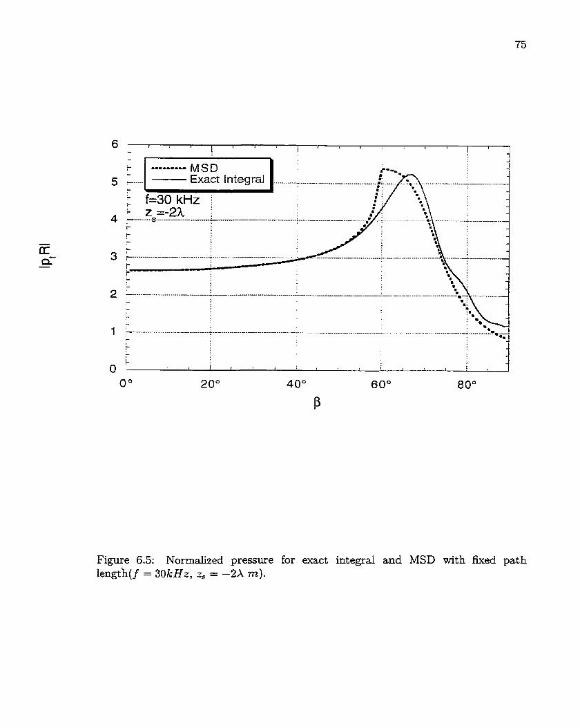
Figure 6.5: Normalized pressure for exact integral and MSD with fxed path lengch(f = 30kHz, z, = -2X m).

Figure 6.6: Normalized pressure for exact integral and MSD with fixed path length(f = 30kHz, z, = -5X m).

Figure 6.7: Normalized pressure for exact integral and MSD with fixed path length(f = IkHz , 2, = -0.U m).

Figure 6.8: Normalized pressure for exact integral and MSD with fixed path length(f = IkHz, z, = -A n).

Figure 6.9: Normalized pressure for exact integral and MSD with k e d path length(f = IkHz, r, = -2X m).

Figure 6.10: Normalized pressure for exact integral and MSD with fixed path length(f = IkHr, z, = -5X m).

Figure 6.11: Normalized pressure for exact integral and MSD with TT varied(f = 30kHz, z, = -0.U m).

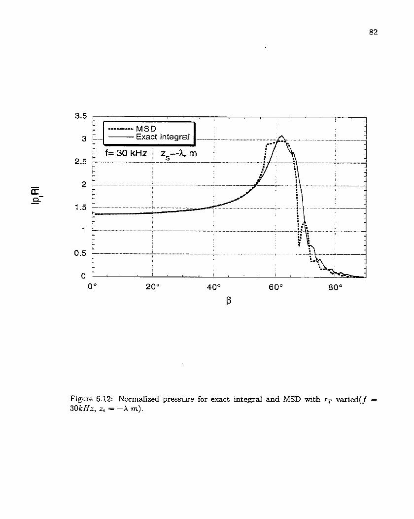
Figure 6.12: Nomalized pressure for exact integral and MSD with r~ varied( f = 30kHz, r, = -A m).

Figure 6.13: Normalized pressure for exact integral and MSD with rr varied(f = 3OkH.q z, = -2X m).

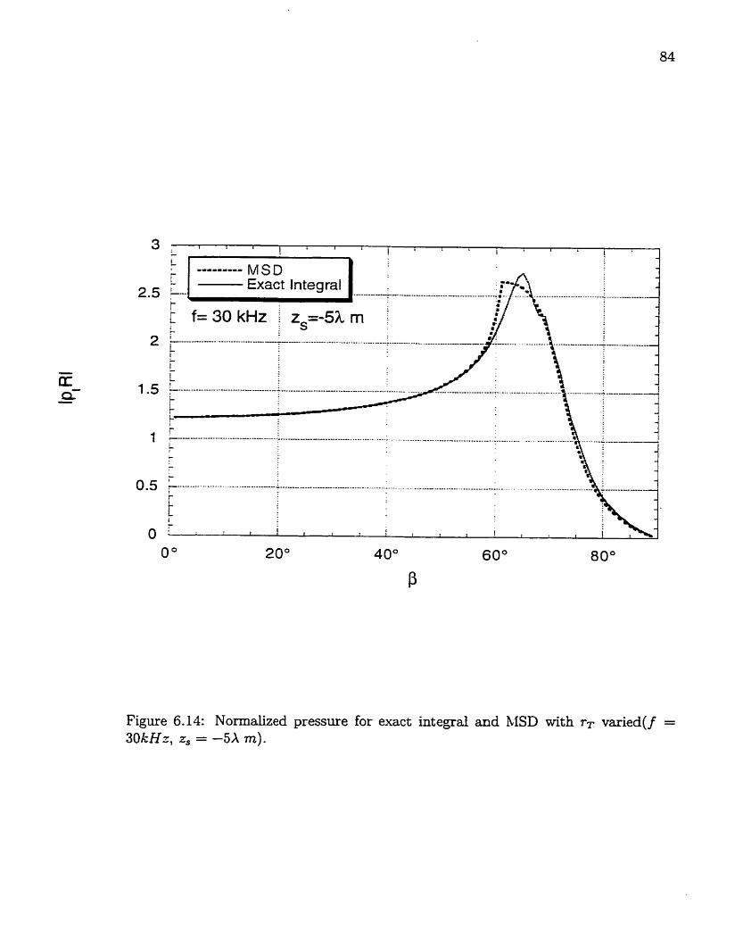
Figure 6.14: Normalized pressure for exact integral and M D with TT varied(f = 30kHz, z, = -5X m).

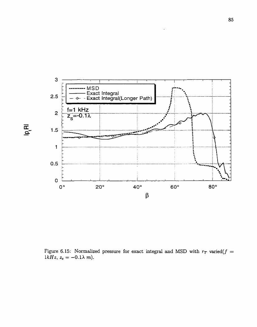
Figure 6.15: Normalized pressure for exact integral and MSD with r~ varied( f = IkHz , zs = -0.1X m).

Figure 6.16: Normalized pressure for exact integral and MSD wit h TT varied( f = LkHz: zs = -A m).

Figure 6.17: Normalized pressure for exact integral and MSD with r~ varied(f = IkHz, z, = -2X m).

Figure 6.18: Normalized pressure for exact integral and MSD with TT varied( f = ZkHz, z, = -5X m).

Fibve 6-19: ,# as a function of yr .

Fi,we 6-20: Refractive and lateral components with TT varied.

Fi,we 6.21: Refractive and lateral components with r~ varied.

L .

1 ; r i ..---,-..-- snell component 5 ; !a, : te,, :

5 +:---.------------;--------.------.------.--;------.------.---. ---.i ---------------- .: 5 .: & t z s =-2h f=30 kHz L ?. . . - ,, - : a

: 8 . : . L : . . . -

----...------------------.; ------------........ i - - - - - - - . - - - - - - - C

m . . . . . . 4 . * - ! i I

< : 8

Ï ; - . . - . . . , . m : 0.5 -.---+-.....-.-....-----.-----.-------. iiiiiiiiiiiiiiiiiiiiiiiiiiiiiii$--* - -.-----.- - 1.-. ---- ..-.-. ---..------------- . . 9 ;

:m. i ! --m. ! - . .

- . -œ . . -11 -9 - ----..r .

'?------ --..----*---.)* "-

O 1 , 7-=------=7--..rCI.--

Figure 6.22: Refractive and lateral components with TT varied.

Chapter 7

Future Work

The decay of the MSD approximation is clearly only of concern for scatterers very

near the wat er-sediment interface. Recallllig that the total backscatt er int ensity is

given by the sum of ail scatterers over the isonified volume, I,, it remains only to

chose a volume of which only a small part is near the interface to improve the original

estirnates.

Presently, numerical est imat es of the exact int egal are computationally inten-

sive. Any suamation over a number of such points would be likewise. The MSD

approximation is faster, usually requiring only one c d to FindRoot provided only

the refracted term is included.

Alternative solutions for Eq. (2 . l ï ) are currently unknown. Solt5ng Eq. (2.15) or

Eq. (3.16) would be ide&. The phase term of each has analytic stationary points and

an MSD contour that behaves similarly to that for Eq. (2.17) when ,L3 < wc. Further-

more, the a w h a r d is not present in either. However, the only saddle point that

the contour passes through is the origin. The integrand from Eq. (2.15) approaches

zero at the origin due to the sin term in the non-exponential factor, whereas Eq.

(2.16) has logarithmic divergence hom the Hankel function. Furthemore, the Tay-

lor expansion of the Hankel function removes the oscillations in the non-exponential

term, placing them instead in the exponent. Thus, the MSD method fails for Eq.

(2.15) and Eq. (2.16). Only numencal methods rem& for solving either equation.

These are as inefficient as solving Eq. (2.17) numerically dong the original contour.

Thus, the MSD approach remains the most promising for obtaining the total

backscatter intensity. Finding the lateral and snell's angles is still more efficient than

numerical integration. Future work dl require the development of an efficient and

effective method to find both angles, and then proceed to obtain solutions for the

total intensity

Appendix A

Alternative Branch Lines for f (S,) Choose the negative real-axis as the branch cut for z1I2. Then if

the branch cut d lie where

is on the negative real-axis.

Let h, be pure real and 11 = q!f+i@". Using the complex representation of sin($)

the branch lines will be given where

sin (23b') sinh(2V) S(k) = = O

2

and

R(k) = n:, - [(sin($') cash($'))* - (cos(@') sinh(q!~"))~] < 0-

S(k ) = O when q' = n7r/2 where n is an integer, and/or +" = O. If 3' = nn/2 and

~" # O, then

by observing that

and

n;, + sinh2($") n even R(k) =

- cosh2(~'') n odd

1 n odd sin2 ( y ) = {

O n even

O n odd cos2 (y) = {

1 n even

If n is even, since sinh2(@"' > O and O < n;, < 1

n;, + çinh2(~~'') p 0

for al1 b. Hoarever,

nZs - cosh2 (qY) < O

since cosh2(d+"' 2 1 for d$" except zero.

If $' # nr/2 and +" = O, then

which is negative provided $ J ~ < +', -& > -$' and $' # nx/3.

If $' = nri/2 and $" = O, then

n even

n:, - 1 n odd

n,, pl 0: however, by definition n:, < 1- In conclusion, f (@) has branch lines for

{ qb : +' = n7i/2; n odd),

Over the given domain on integration

{-sr12 5 ?,b' 5 x/2 and - < qjn < 00)

@' = nn/2 introduces branch lines a t $' = f n/2. The second two conditions simply

create lines on the red-axis extending from ec to positive infinity and -WC to negative

infinity.

Appendix B

Alternat ive Solut ions Alternative methods to computing Eq. (2.17) have yet to be found. Chapter

(5) dernonstrated the effectiveness of the MSD for angles aside kom those near critical.

The decay was largely dependent upon the depth of the source. A technique effective

for all range of angles would be ideal.

One alternative approach deserves some discussion. Consider Eq. (2.15) with

respect to Eq. (2.17). Brekhovskikh[3] performs a Taylor expansion of H;') to obtain

Eq. ( 7 ) . Hence, Eq. (2.17) is an approximation of the original pressure, possibly

increasing the error of the MSD approach and that from ~ a t h e m a t i c a ' s ~ ~ NIntegrate,

the only means of cornparison.

Eq. (2.16) results hom replacing the Bessel function of Eq. (2.15) with a mm

of Hankel functions. The Hankel functions have logarithmic divergence at the origin

and a branch line typicdy chosen along the negative red &S. Altematively, the

Bessel function shares the same branch line, but contains no singularities[g]. Hence,

Eq- (2.15)

provides an exact represent ation for the pressure with potentially the least patholog-

ical features.

Examining the branch lines of Eq. (2.15), this proposition is supported. First the

non-exponential factor does not contain Next consider the exponential term

dn:, - sin2 0. Expanding sin 8, let

g(0) = {nk - [(sin 8' cosh O")* - (COS 8' sinh 0")*]) + i(sin 28' sinh 2 0 M ) / 2 ) .

The brandi points will be given by g(0) = O. Qg(0) is identicaIly zero when 19' =

0, &7r/2 and/or 8" = 0. If 8' = f7t/2 and 8'' # O, then

2 " Rg(9) = n L - cosh O

which is zero when

O" = ~osh-~(n,,).

If 0' = O and O" # 0, then

This can never be zero as both nzw and sinh2 8" 2 0.

If 0" = O and 8' # O, &ir/3, then

9 2 f Rg (9) = n, - sin 0

which is never zero-

If 6" = O and 0' = &7r/2, then

Lastly, if both 0' and 8" are zero

Hence, the branch points are given by I r / 2 + i cosh-' n,,.

Next consider the braxich lines if the cut lies along the positive real axis, or where

Rg(e) < o. The following three cases are considered.

First, if 0' = 0, +7r/2 and 8" # O , then

The term n k - cosh2 6" can be only less than zero when

Secondly, if 0' # 0, =tir/? and 0" = O, then

sg (e) = n;w - sin2 e

which is never negative as O 5 sin# 5 1 for -7r/2 4 O' $ i i /2-

Lastly, if 6' = 0, f sr/2 and O" = O, then

None of the above will ever be negative.

Thus, the branch lines are given by

{O' = f 7r/2 and 8" > cosh-' n,).

For Eq. (2.15) Mathematica's choice of cut for the square root is clearly bet-

ter than Brekhovskikh7s[3]- Furthemore, as discussed in Appendix (A), the term

Jn:, - sin2 O in the transmission coefficient merely introduces cuts that coincide

with those dong &7r/2. This much simplifies the numerical f i cu l t i es associated

with frequently changing sheets. The four familiar poles from the same terni remain

unchanged.

Next consider the phase term

The derivative of f (8) is giwn by

z, cos 0 sin 9

Clearly O will always be a root of f '(O). The remaining roots are given by

If z, = z, the above simplifies to sin2 0 + cos2 9 # 0. Under these circumstances the

origin is the only stationary point. Otherwise, after carefd simplification

is obtained.

If z, > [ % 1 7 the right-hand side of the above is pure real. Othernrise it is pure

imaginary. For the former, expanding cos 0 in its complex representation

and

sin 9' sinh 6" = O.

If 0" = O and 8' # O, tben sin O' sinh 8" is identically zero and cos 8' cosh 8" becomes

1/2

cos*' = * ( -= ,2na, 12 - - 72 1)

Since O < cos 0' 5 1 for - ~ / 2 5 8' 5 7ï/2 ody the positive case needs to be considered.

This requires

If O " # O and 0' = O , then

Since coshû" 2 I once again only the positive case needs to be considered. This

requires

If n:w = (&/z.)~, then 6' = 8" = O which again corresponds to the origin.

is pure imaginary. Thus, the two equations

and 1/2

sin of si* eM = * (-, n:~ - f ) 2 - 2,- must be solved.

cos 9' cosh O" is only zero when 0' = i.?r/2. If O' = ~ / 2 , then sin O' sinh O" becomes

If 8' = -7r/2, the same equation must be solved. In both cases the two solutions are

Summarizing the above, first, the origin is always a stationary point. If r, > /z,I, there can be two additional points

1/2

0 = COS-' 's -2 , -&:) -2

2 if n,, 5 ( t ; / ~ , ) ~ . If ry < IZ,~, there are four stationary points 9' = ~ / 2 , O" > 0,

O' = - ~ / 2 , 8" > 0, 9' = r / 2 , 0" < O and 8' = -?r/2, 8" < O, where

To obtain the MSD contour

3 f (O) = constant = c

must be solved, which after some simplification becomes

-zs cos 8' cosh 0" + !R(zw\jn~, - sin2 O) = c.

Since all of the stationary point(s) lie on the axes, the behaviour of the contour

as a -, O and O" + O must be examined. As 0' -, 0,

3f (8) - -r, cosh0" + & i R J m .

Using the identiw

s k i 0 = isinh0

t his simplifies t O

-rs COS^ eu + &RJ-

Letting the above equd the constant c yields

for a l l O".

5 f (0) - -2, cos 0' + z , , ,~ \ jn~, - sin2 8'

since n h > sin2 Of for al1 0'. Letting the above equal the constant c yields

2 2 COS 0' (cos B'(Z? - z,) + 2~2,) = zy (n, - 1) - c2

Since O 5 cos 0' 5 1 for -?r/2 5 Of 5 a l 2

for alle'.

However , since

both

cosh Or' (cosh 9"(r:- - r:) + 2%)

and

O 5 cos #(COS ef (zQ - z:) + ~cz,)

must be less than or equal to and greater than or equal t o

Both inequalities can ody hold when

-. c2 + Zcz, + (z: - ryn?,) = O-

This quadratic has the two solutions

The second of these corresponds to f (O). Hence, the contour will start at - ~ / 2 - ioo

and approach the real and imaginazy axis as it approaches the origin.

Clearly? for the set of stationary points and the choice of branches above, the MSD

approximation can be easily applied to Eq. (2.15). Furthermore, the contour does

not cross any branch points, dowing ease of calculation when performing numerical

integration. Unfortunately, the difficdty of applying the technique lies in the non-

exponential factor. As 0 + 0, sin + O and the MSD approximation will be zero.

Hence, only numerical methods remain for determinhg the exact integral. Nonethe-

less, Eq. (2.15) has a shorter path length than Eq. (2.16)- hthermore , the absence

of the Hankel function prevents logarithmïc divergence at the origin. Thus, Eq. (2.15)

remains potentidy the most straightforward integrand to evaluate numerically-

Appendix C

Arfken's MSD Approach Following the examples given in Arfken [Z] for the asymptotic forms of the Han-

kel and factorial functions: a three step algorithm was developed by the author to

determine the MSD approximation.

Denoting 20 as a stationaq point, fkst recall that the phase of the contour, a,

must be chosen such that r - zo = Je'" at the saddle. M e r chosing a small6, a can

be obtained by solving

If there is more than one a, then that which makes the real part of f (6eiQ + zo) a

minimum must be chosen. This corresponds to the path of steepest descents[2].

Correspondingly, first

must be solved. Provided 6 < 10-'O, the zeros typicdy lie in the intervals [O, ~121,

[7r/2, T ] , [T. 3i;/2] and [3~/2,2n]. This can be seen by plotting the above hinetion

which behaves like sin between O and 27r. Next, the phase that makes

Rf (Scosa + Sr, f i h i n a )

a minjmrim is chosen. The resulting phase is used in the approximation-

Values of J between 10-5 and 10-~ typically resulted in an approximation similar

to Brekhovskikh ls and those from the numencal integrations. However, A*ken[2]

provides no advice as to the magnitude of 6. Hence, his technique was not pursued

when examining the breakdown of the MSD approximation near the critical angle.

It is clear why the approximation breaks down for negligible values of 6. As 6 -t O

since bot h sin @ and cos zir are in [- 1,1] for cr E [O, 2 ~ 1 . Consequently. any a will solve

this equation.

Ar£ken['L] introduces the term 6eia not only to find a, but also to d o w for series

expansions of

8 f (6 cos a + $+ + id sin a).

Terms of order 63 and higher are neglected. This qproach d o w s for considerable

simplification when f (r) = 1/2 (z - 1/z) and ln r - t for the Hankel and factorial

examples: respectively. However, R f (6eia + &) doeç not yield such simplification

even if Je'" is replaced by its trigonometric form b(cos a: + i sin a). Furthermore,

MathematicaTM allows numerical solutions for a as opposed to the analytical results

obtained by Arfken.

Appendix D

Sample ~ a t hemat kaTM Code Argument function that will produce the branch cuts

used by Brekhovskikh dong the positive real axis

Clear [BrekArg] ;

BrekA.rg[x- ] :=

IflIm[x] 2 0 ,ArcCos [Re[x] / Abs[x]] , 2*Pi-ArcCos [Re[x] /Abs [x]]]

Compile [{x) , Br ekAr g [x] ] ;

Square root with Brekhovskikh's choice of cuts

Clear [SqrtBrek] ;

SqrtBrek[x- ] := (8=(BrekArg[x] /2);

Return[N [Sqrt [Abs [x]] * (Cos [O] +I*Sin[B]) ,1011) ;

Compile[{x), SqrtBrek[x]];

Constants

Turn off the messages from FindRoot

Off [FindRoot : :fisec] ;

Off [FindRoot ::frdig] ;

O£F[FindR.oot: :fimp] ;

Function for hding snell's law angle

Arguments are rr, zw and zs

Clear [S nell] ;

Snell[rT- ,zs- ,zw- ]:=(

(* derivative function *)

(* Note:for incident angle in water *)

(* ~ rather that that f n sediment *)

Clear [fder] ;

fder [x- ] :=(rT*Cos [XI-~v*Sin[x] ) *Sqrt [n&s-~in[x] *] + (zs*Sin[x] *Cos[x] ) ;

Compile [{x) , fder [x]] ;

(* h d the root *)

snell=x /. FindRoot [fder[x] ==O, { X , O , $ ~ ) ,

MaxIterations- 150O,WorkingPrecision+l 5,

AccuracyGoal~15,Compiled-True] ;

(* return estimate *)

Ret urn[snell] ) ;

Compile[{rT,zs,mv),Snell[rT,zs,zw]];

Function for h d i n g lateral(evanescent ) angIe

(* derivative function *)

(* Note:for incident angle in water *)

(* $ rather than that in sediment *)

Clear[fBrekder] ;

fBrekder[x_ ]:=(rT*Cos[x]-zw*Sin[x])*

SqrtBrek[n&-Sin [~]~]+zs*Sin[x]*Cos[x]);

Compile[{x) ,fBrekder[x]] ;

(* use 0 plus a small complex number for *)

(* one of the starting values *)

lateral=

x /. FindRoot[fBrekder[x] == O,

{x,P + 10-6*I,$c - iO-8*I}7

MaxLterations+3000,WorkingPrecision+20,

AccuracyGoal+20,Compiled-t~ue];

Return [lateral]) ;

Cornpile[{rT,zs,zw),Lateral[rT,zs,zw]];

Transmission coefficient

Clear [TS W] ;

TSW[x- ]:=(2*msw*Cos[x])/

(msw*Cos[x]+SqrtBrek[n&s-Sin[x]']);

Compile [{x} ,T§ W[x]] ;

Non-exponential te- in integrand

Terms for the snel17s angle MSD contribution

Clear [Fsnell] ;

Fsnell[x- ]:=TSW[x]*SqrtBrek[Sin[x]] ;

Compile[{x),Fsnell[x]] ;

Terms for the lateral angle MSD contribution

(use the integrând in terms of 11, instead)

Function for finding the MSD approximation

(* multiplier from integrand *)

ConstantMultiplier=

N[Exp[I*Pi/4]*Sqrt[ks/(2*Pi*rT)],10];

(* phase terms used for snell's angle *)

Clear [fsnell] ;

fsnell[x- ]:=

I*(rT*Sin[x]-zs*Cos[x]+zw*SqrtBrek[n~wSin[x]']) ;

(* second derivative of phase term *)

Clear[fder2snell] ;

fcier2snell[x- ]:=I* (zsCos[x]-rTSin[x]-

(23/2z~(~in[~]4+~os[2x]n~w) / (-I+COS[PX] +2n&#/*));

(* non-exponential term *)

Clear[Phi~] ;

Phi0 [x- ]:=N[Fsnell[x]*SqrtBrek[-2/(I*fder2snell[x])] ,201;

(* snell's law angle *)

snell=Sriell[rT,zs,mvl;

(* convert to angle in sediment *)

t hetasnell=ArcSin[nsw *Sin[snell]] ;

(* snell contribution *)

snellcontribution = ConstantMultiplier*

NIExp[ks*fsnell[thetasd]] *Sqrt [Pi/ks]

(* phase term used for lateral angle +)

Clear [flateral] ;

flateralix- ]:=I*(rT*Sin[x]+zw*~os[x]-zs*~qrtBrek[n&~-Sin[x]~]);

(* include lateral contribution if required *)

IflB>+c&&Im[flaterd[sneU]] <Sqrt[rT2+zw2]), (

(* obtain lateral angle *)

lateral=Lateral[rT, zs, zw] ;

(* find lateral contribution *)

denominator[x- ]:=Sqrt [rT] *Sqrt [rT*Sin[x]+zw*Cos[x]-

~s*((Cos[2*x]/Sqrt[n&,-Sin[x]~])+((Sin[2*~]~)/ 2 3/2 (4*(n~,~-sin[x1 ))II;

msd = msd + lateralContribution;)];

Switch off rnwxling messages from NIntegrate

Transmission t errn for exact pressure

Clear[TS Wexact] ;

TS Wexact [x- ]:=(2*msw*Cos[x])/(msw*Cos[x]+

sqrt [n&-Sin[x]']) ;

Compile[{x) ,TS Wexact [x]] ;

Function to obtain exact pressure

(* phase term in integrand *)

Clear[f] ;

qx- ] :=I*(zw*Sqrt [n&-Sin[~]~]-zs*~os[x]);

Compile [Cxl7r[xll;

(* term in Bessel function *)

Clear[u] ;

u[x- ]:=rT*ks*Sin[x];

com~wCxl,u[xll; (* non-exponential term in integrand *)

Clear[Fexact] ;

Fexact[x- ] :=BesselJ[D,u[x]]*TSWexact[x]*~i~~[x];

Compile[{x) ,Fexact [x]] ;

(* integrand *)

Clear[integrand];

integrand[x- ]:=Exp[ks*flx]] *Fexact [x] ;

Compile[{x) ,integrand[x]] ;

(* numerical approximation from NIntegrate *)

Ci =NIntegrate[integrand[x],

{x,Pi/2-T*Pi,Pi/2-I*ArcCosh[nsw],Pi/2),

MaxRecursion+l5, WorkingPrecision+ 15 , Compiled-t True] ;

Cz =NIntegrate [int egrand[x] , {x,Pi/27+c,O), MaxRecursion+l5,WorkingPrecision+ 15,

Compiled-t True];

Code to obtain MSD approximation and exact pressure

at one degree intervals of /? by vasying TT

Source depth set to -2X

Print [i," " ,Re[msdresult] ," ,Im[msdresult] ," " , Re [exactresult] ," " ,Im[exactresult]] ;

Bibliography

[l] M. XBRAMOWITZ, A S D 1. .A. STEGCS HandbooP of Mathematical Functions, Dover, New York, 1972,

[2] G . ARF K E N Mathematical Methods for Physicists, Third Edition. Academic Press. 1985.

[3] L. M. BREKHOVSKIKH Wawes in Layered Media, Second Edi t ion ilcademic Press. London, 1980.

[4] 4. B. COPPENS: A. R. FREY, L. E. KINSLER, AND J - V. SANDERS Fundamentals of Acowtics, 3rd. Ed., John wiley & Sons, Inc,, New York: 1982.

[J] P . H ~ ~ ~ ~ E x a m i n a t i o n of Acowtic Backscatter f iom an Inhomogeneous Volume Beneath a Planar Interface, Ph-D. Thesis, Bath University, U K , 1988.

[6] P . C . HINES Theoretical Model of Acorstic Backscatter From a Smooth Seubed, Journal o f the Acoustical Society o f America, S8(l), 324-334. 1990.

[7] P. C . HIN ES Theoretical Model of In-Plane Scatter From a Srnooth Sedirnent Seabed, Journal of t h e Acoustical Society o f Arnerica, 99(2), 836-844, 1996.

[SI B. P. P A L K A A ~ Introduction to cornplex Function Theory, Springer-Verlag, New York, 1991.

[9] M . R. SPIEGEL Theory and Problems of Complex Variables, Schaum, New York , 1964.

[IO] S. w o ~ ~ ~ ~ ~ The MathematicaTM Book, 3rd. Ed., Wol f iam Media, Illinois, 1996.