Embed Size (px)
Citation preview
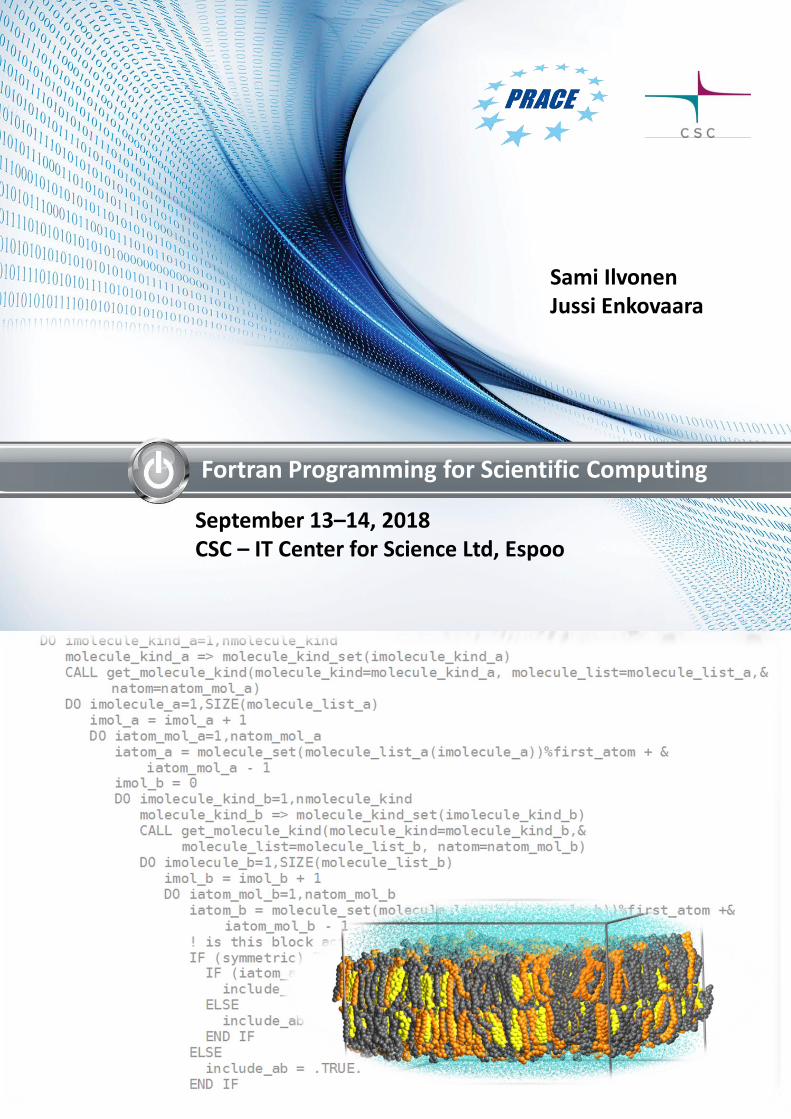
Fortran Programming for Scientific Computing
Sami IlvonenJussi Enkovaara
September 13–14, 2018CSC – IT Center for Science Ltd, Espoo

All material (C) 2009-2018 by CSC – IT Center for Science Ltd.This work is licensed under a Creative Commons Attribution-NonCommercial-ShareAlike 3.0 UnportedLicense, http://creativecommons.org/licenses/by-nc-sa/3.0/
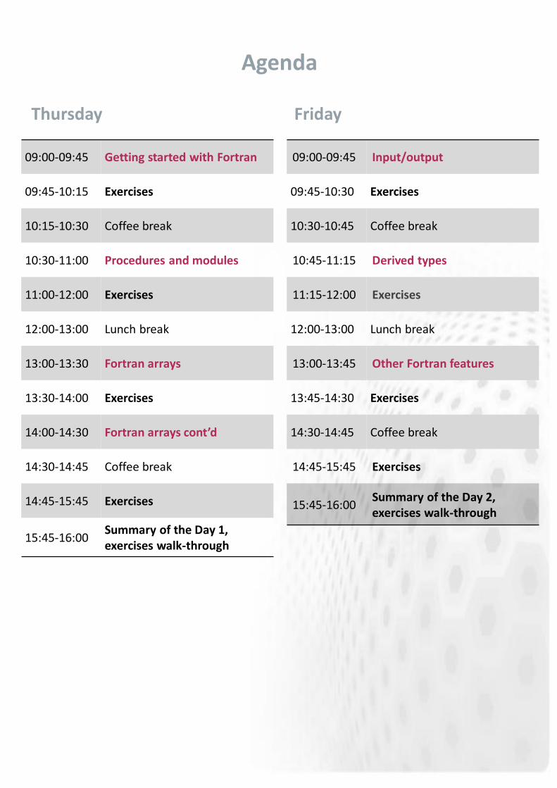
Agenda
Thursday
09:00-09:45 Getting started with Fortran
09:45-10:15 Exercises
10:15-10:30 Coffee break
10:30-11:00 Procedures and modules
11:00-12:00 Exercises
12:00-13:00 Lunch break
13:00-13:30 Fortran arrays
13:30-14:00 Exercises
14:00-14:30 Fortran arrays cont’d
14:30-14:45 Coffee break
14:45-15:45 Exercises
15:45-16:00Summary of the Day 1, exercises walk-through
Friday
09:00-09:45 Input/output
09:45-10:30 Exercises
10:30-10:45 Coffee break
10:45-11:15 Derived types
11:15-12:00 Exercises
12:00-13:00 Lunch break
13:00-13:45 Other Fortran features
13:45-14:30 Exercises
14:30-14:45 Coffee break
14:45-15:45 Exercises
15:45-16:00Summary of the Day 2, exercises walk-through
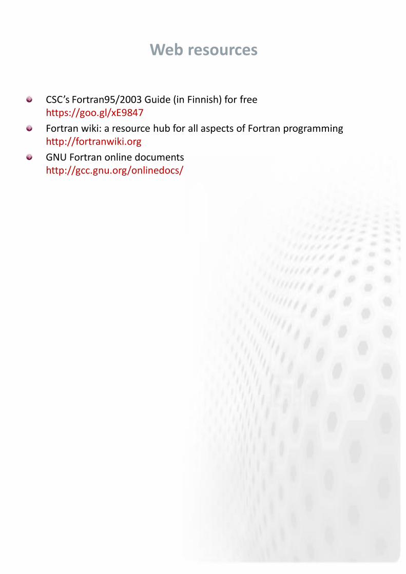
Web resources
CSC’s Fortran95/2003 Guide (in Finnish) for freehttps://goo.gl/xE9847
Fortran wiki: a resource hub for all aspects of Fortran programminghttp://fortranwiki.org
GNU Fortran online documentshttp://gcc.gnu.org/onlinedocs/

Exercises
General instructions Use the local workstations for the exercises.
All source codes are in a github repository https://github.com/csc-
training/fortran-introduction and they can be downloaded as
git clone https://github.com/csc-training/fortran-introduction.git
All exercises are under their own subdirectory which contains both skeleton
codes and model solution (under solution folder)
For every given exercise you are supposed to edit or correct the skeleton
source code. Look for TODO-tags in the source and provide a fix.
GNU compiler is used by default and the compiler command is gfortran.
Example command:
gfortran -o hello hello.F90
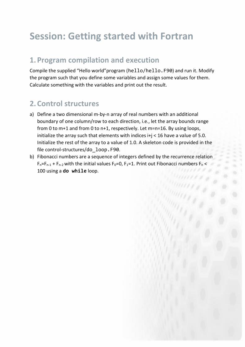
Session: Getting started with Fortran
1. Program compilation and execution Compile the supplied “Hello world”program (hello/hello.F90) and run it. Modify
the program such that you define some variables and assign some values for them.
Calculate something with the variables and print out the result.
2. Control structures a) Define a two dimensional m-by-n array of real numbers with an additional
boundary of one column/row to each direction, i.e., let the array bounds range
from 0 to m+1 and from 0 to n+1, respectively. Let m=n=16. By using loops,
initialize the array such that elements with indices i+j < 16 have a value of 5.0.
Initialize the rest of the array to a value of 1.0. A skeleton code is provided in the
file control-structures/do_loop.F90.
b) Fibonacci numbers are a sequence of integers defined by the recurrence relation
Fn=Fn-1 + Fn-2 with the initial values F0=0, F1=1. Print out Fibonacci numbers Fn <
100 using a do while loop.
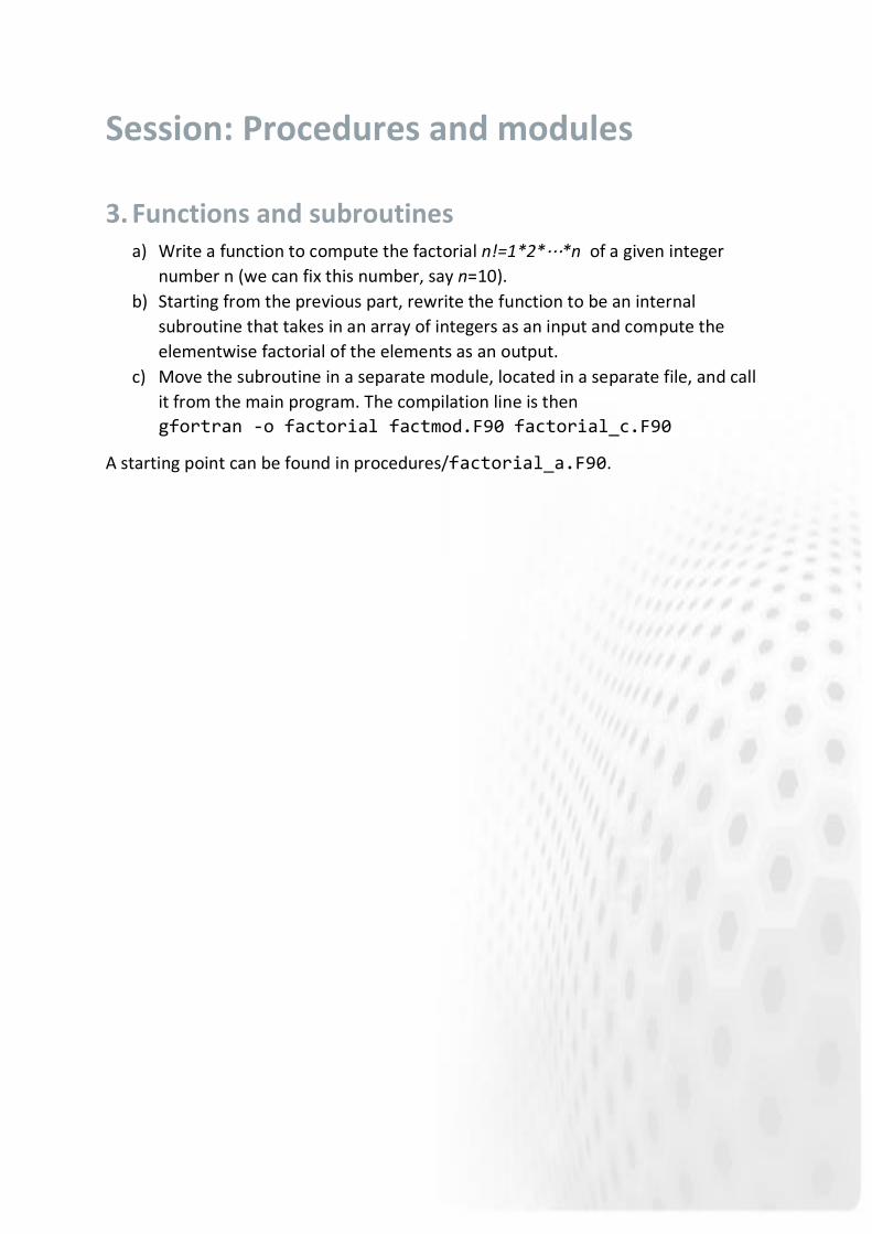
Session: Procedures and modules
3. Functions and subroutines a) Write a function to compute the factorial n!=1*2*⋯*n of a given integer
number n (we can fix this number, say n=10).
b) Starting from the previous part, rewrite the function to be an internal
subroutine that takes in an array of integers as an input and compute the
elementwise factorial of the elements as an output.
c) Move the subroutine in a separate module, located in a separate file, and call
it from the main program. The compilation line is then
gfortran -o factorial factmod.F90 factorial_c.F90
A starting point can be found in procedures/factorial_a.F90.
Session: Fortran arrays
4. Loops, arrays and array syntax a) Write a double do-loop for evaluating a Laplacian of a two-variable function
using the finite-difference approximation
As an input, use the array with the same initial values as in Exercise 2 (or start
from the skeleton loops-arrays/loops_a.F90). Evaluate the Laplacian
only at the inner 16x16 points, as the outer points are used as boundary
condition. As a grid spacing, use Δx=Δy=0.01.
b) Instead of using a double do-loop, use array syntax to compute the values of
the Laplacian. Dynamic arrays and intrinsic functions
5. Dynamic arrays and intrinsinc functions a) Define a matrix A which should be dynamically allocatable. Then allocate the
matrix with sizes read in from the user input and fill the matrix with random
numbers using the array intrinsic function random_number.
b) Then use suitable array intrinsic functions to print out the following details:
What is the sum of elements across the 2nd dimension of A?
Find the location coordinates of the maximum elements of A.
What is the absolute minimum value of the array A?
Are all elements of A greater than or equal to zero?
How many elements of A are greater than or equal to 0.5?
There is a skeleton code being provided in dynamic-arrays/array.F90.
𝛻2 𝑢(𝑖, 𝑗) =(𝑢(𝑖 − 1, 𝑗) − 2𝑢(𝑖, 𝑗) + 𝑢(𝑖 + 1, 𝑗))
(𝛥𝑥)2+
(𝑢(𝑖, 𝑗 − 1) − 2𝑢(𝑖, 𝑗) + 𝑢(𝑖, 𝑗 + 1))
(𝛥𝑦)2

Session: Input and output
6. File I/O Implement a function that reads the values from a file bottle.dat. The file contains a
header line: “# nx ny”, followed by lines representing the rows of the field. A
skeleton code is provided in io/io.F90.
Once you have completed the implementation, you can build the full program (io)
with the provided Makefile by executing
$ make
The program writes out the data as png-image.

Session: Derived types
7. Derived types Define a derived type for a temperature field. Do the definition within a module (let’s
call it laplacian_mod for the purpose of a subsequent exercise). The type has the
following elements:
Number of grid points nx (=number of rows) and ny (=number of columns)
The grid spacings dx and dy in the x- and in the y-directions
An allocatable two-dimensional array containing the data points of the field.
Define the real-valued variables into double precision, using the ISO_FORTRAN_ENV
intrinsic module. An example is in derived-types/solution/fieldtype.F90.
8. Derived types and procedures Let us extend the module started in Exercise 7 by adding the initialization of the two-
dimensional array (Exercise 2), finite-difference Laplacian (Exercise 4) into their own
functions, which now take the type representing the temperature field as an input.
Session: Afternoon exercises
9. Command line arguments Modify the given template so that the command line arguments are read in the
following way:
1. If no command line arguments are given, program prints out a short notice.
2. If one argument is given, it is interpreted as a string and the value is stored to
a variable called input_file.
3. If two arguments are given, first argument is interpreted as in case 2 and the
second argument is treated as an integer value and stored to a variable called
nsteps.
4. If three arguments are given then they all are interpreted as integers and
values are stored to variables rows, cols and nsteps in this order.
10. (BONUS) Heat equation Finalize the implementation of our two-dimensional heat equation solver (see the
Appendix) by filling in the missing pieces of code (marked with “TODO”) in heat-
equation/main.F90. You can compile the code with the provided makefile.
a) The main task is to write the procedure that evaluates the new temperature
based on previous one (called “evolve” here), utilizing the existing
implementation (Exercise 4) for the Laplacian:
The skeleton codes readily contain suitable values for time step Δt and for the
diffusion constant α. Run the code with the default initialization.
b) Another task is to implement a reading in of the initial field from a file (cf.
Exercise 6). Test the implementation with the provided bottle.dat.
Appendix: Heat equation solver
The heat equation is a partial differential equation that describes the variation of
temperature in a given region over time
where u(x, y, z, t) represents temperature variation over space at a given time, and α
is a thermal diffusivity constant.
We limit ourselves to two dimensions (plane) and discretize the equation onto a grid.
Then the Laplacian can be expressed as finite differences as
Where ∆x and ∆y are the grid spacing of the temperature grid u. We can study the
development of the temperature grid with explicit time evolution over time steps ∆t:
There is a solver for the 2D equation implemented with Fortran (including some C for
printing out the images). You can compile the program by adjusting the Makefile as
needed and typing “make”.
The solver carries out the time development of the 2D heat equation over the
number of time steps provided by the user. The default geometry is a flat rectangle
(with grid size provided by the user), but other shapes may be used via input files - a
bottle is give as an example. Examples on how to run the binary:
./heat (no arguments - the program will run with the default arguments:
256x256 grid and 500 time steps)
./heat bottle.dat (one argument - start from a temperature grid provided in
the file bottle.dat for the default number of time steps)
./heat bottle.dat 1000 (two arguments - will run the program starting from a
temperature grid provided in the file bottle.dat for 1000 time steps)
./heat 1024 2048 1000 (three arguments - will run the program in a
1024x2048 grid for 1000 time steps)
The program will produce a .png image of the temperature field after every 100
iterations. You can change that from the parameter image_interval. You can visualize
the images using the command animate: animate heat_*.png.